A Unified Framework for Optimization and Analysis of Fractional-Order Chaotic Systems

Abstract

Maximizing the dominant Lyapunov exponent ${\lambda }_1$ of an incommensurate fractional-order chaotic system, while respecting the dynamical conditions for a strange attractor, is a non-convex, gradient-free problem on a history-dependent landscape. Existing metaheuristic studies typically use hard-cutoff penalties that distort the fitness landscape and integer-order Lyapunov estimators that can be biased for strongly fractional regimes. This paper presents a constraint-faithful optimization framework combining (i) subtractive-hinge penalties that vanish on the feasible set, (ii) a memory-consistent Grünwald–Letnikov variational Lyapunov estimator with adaptive tail-sum truncation, (iii) joint search over parameters and incommensurate orders by the Marine Predators Algorithm, and (iv) a fractional conditional Lyapunov exponent (FCLE) that recovers the integer-order limit. Applied with a fixed configuration to the fractional-order Lorenz, Ma–Chen financial, Iqbal–Wang, and Hyper–Chen systems, the framework converges to feasible attractors with enlarged Lyapunov spectra. Dissipativity is rigorously verified; all selected optima have strictly negative Lyapunov trace at the reported precision. FCLE analysis on the optimized Lorenz attractor recovers the integer-order identity $c_{min}={\lambda }_1$ under full-state coupling, and shows that single-state x-coupling raises the threshold to ≈9${\lambda }_1^{*}$. The optimized fractional-order Lorenz attractor is employed as the random-number generator of a recent chaos-based image-encryption scheme, where it yields strong statistical results across standard benchmarks.

1. Introduction

Chaotic dynamical systems combine deterministic evolution with sensitivity to initial conditions and aperiodic, bounded trajectories. They are widely used in chaos-based communications, pseudo-random number generation, and image-based information-hiding pipelines [1,2,3,4,5,6]. Earlier circuit-oriented studies also showed that differential-equation-based chaotic generators and controllable multiscroll attractors can provide practical random-signal sources for digital and hardware-oriented security applications [2,7]. Fractional-order chaotic systems have also become a widely used entropy source for image-encryption pipelines, including synchronization-driven schemes in which a drive–response pair (e.g., delayed fractional-order neural networks under intermittent control) generates the keystream used in a semi-tensor-product cipher [8]. Such schemes exploit the additional memory and parameter freedom of the fractional setting, and they motivate the synchronization analysis and application demonstration of Section 5. In each of these contexts, the empirical quality of the downstream pipeline tracks the dynamical complexity of the underlying source, typically measured by the dominant Lyapunov exponent ${\lambda }_1$, the number of positive exponents, or the Kaplan–Yorke dimension [9,10,11,12].

Local fractional-derivative formulations have also been applied to the Lorenz system to study how the differentiation order reshapes the Lyapunov spectrum and Kaplan–Yorke dimension while recovering the integer-order limit [13]. By contrast, the present work retains the nonlocal Grünwald–Letnikov memory, which is the regime in which the incommensurate-order coupling investigated here arises. Replacing integer-order derivatives with fractional ones introduces nonlocal, history-dependent dissipation that enriches the dynamical landscape. Incommensurate fractional-order chaotic systems can sustain chaos at parameter values inaccessible to their integer-order limits and exhibit attractors of larger Kaplan–Yorke dimension at reduced effective order [14,15,16,17]. The Grünwald–Letnikov (GL) discretization that underpins most numerical work on fractional chaos is a backward convolution over the entire trajectory history. More generally, the numerical realization of differential-equation-based chaotic generators can alter the measured chaotic response, including the maximum Lyapunov exponent and autocorrelation behavior [7]. Consequently, inner-loop estimators that ignore fractional memory may return biased Lyapunov exponents in the incommensurate regime [17,18]. The search space is correspondingly enlarged: a faithful optimization must vary both the system parameters and the incommensurate fractional orders $\mathbf{q}=(q_1,\dots ,q_n)$, turning a three- or four-parameter sweep into a six- to nine-dimensional non-convex search on a memory-dependent landscape [19,20]. Many population-based metaheuristics have been applied to this class of problems on integer-order systems, including differential evolution, particle swarm optimization, and the competitive swarm optimization algorithm [21,22]. Chaotic variants of metaheuristics such as flower pollination and grey wolf optimization have also been used for fractional-order parameter extraction problems [23], while the Marine Predators Algorithm (MPA) has been applied to different classes of problems involving fractional derivatives [24,25,26].

Despite considerable activity in this area, three methodological gaps still limit the scientific interpretability of the resulting Lyapunov exponent values. These gaps motivate the present framework.

• The conditions that a chaos-maximizing solution must satisfy (dissipativity, boundedness, asymptotic stability of the Lyapunov estimate, and the dimension-appropriate chaotic signature) are typically imposed through hard cutoffs that assign a large constant value to infeasible candidates and use the merit term otherwise. Such cutoffs create flat plateaus and discontinuous cliffs that trap population-based optimizers and leave an open path into infeasible high-${\lambda }_1$ regions, where the integrator reports a large positive exponent for trajectories that are in fact unbounded, numerically unresolved, or of the wrong chaotic class [16].
• Many studies evaluate the objective with an integer-order routine, in which the extended Benettin–Wolf algorithm collapses the row-dependent memory of the variational equation into a single integration. This approximation is acceptable near the integer-order limit but can be biased in the strongly fractional, incommensurate regime targeted here [17], causing the optimizer to effectively maximize the wrong quantity.
• The system parameters and the order vector $\mathbf{q}$ are often fixed or optimized in alternation [16], so the coupling between fractional memory and parameter scale, which is precisely where incommensurate fractional chaos arises, is never exposed to the optimizer.

A direct consequence of these gaps is that absolute record ${\lambda }_1$ values reported across different studies are not directly comparable: ${\lambda }_1$ scales with the attractor extent itself, and the bounds, fractional-order settings, and feasibility constraints differ from study to study [16,21], so a larger number need not indicate a better method. The framing of this paper is therefore methodological rather than record-seeking.

This paper presents a unified framework that closes the three gaps above. The novelty lies in the integration of constraint-faithful feasibility handling, a memory-consistent inner-loop Lyapunov estimator, and joint parameter-order optimization within a single framework. The framework is further extended to a synchronization diagnostic. Concretely, the contributions are:

• A Penalized Marine Predators Algorithm (P-MPA) in which each necessary dynamical condition is encoded as a subtractive hinge that vanishes exactly on the feasible set. Each hinge supplies a descent direction toward feasibility and contributes nothing once the candidate becomes feasible, so the merit landscape near the optimum is left undistorted; this is the precise sense in which the scheme is constraint-faithful.
• A memory-consistent inner-loop estimator in which the GL variational Lyapunov estimator of Li et al. [17] is applied row by row, preserving the row-dependent memory of the incommensurate variational equation. Therefore, the quantity maximized within the optimization loop is the same as the quantity verified offline.
• Joint optimization of parameters and orders. The system parameters and the incommensurate fractional orders are optimized inside a single six- to nine-dimensional decision vector, exposing the parameter–order coupling that alternating schemes miss.
• A fractional conditional Lyapunov exponent (FCLE). The variational construction is carried to the drive–response error system, generalizing the Pecora–Carroll threshold [27] to incommensurate GL dynamics and recovering the integer-order limit as $q_i\to 1$.

A further integrative contribution is generality: the same outer-loop, inner-loop estimator, and penalty design are applied without modification, apart from one threshold substitution, across four structurally distinct systems, demonstrating that the framework is system-independent rather than tuned to a specific example.

The framework is applied to four chaotic systems chosen to span a representative range of fractional chaos: the fractional-order Lorenz system [14], used as a three-dimensional methodological anchor with a single positive exponent; the three-dimensional Ma–Chen financial system [28,29], which exhibits low-amplitude finance-motivated chaos; the four-dimensional Iqbal–Wang hyperchaotic system recently introduced in [30]; and the four-dimensional Hyper-Chen hyperchaotic system [31]. Under a single fixed configuration, the framework converges to attractors with enlarged Lyapunov spectra relative to the canonical regimes. A compact application demonstration integrates the optimized Lorenz attractor into a chaos-based pseudo-random number generator and a two-stage image-encryption pipeline.

The remainder of the paper is organized as follows. Section 2 reviews the GL discretization, the adaptive memory-truncation criterion, and the memory-consistent variational LE estimator. Section 3 develops the P-MPA framework on the fractional-order Lorenz system. Section 4 applies the framework to the financial, Iqbal–Wang, and Hyper-Chen systems and consolidates the cross-system signature. Section 5 reports the FCLE synchronization analysis and the application demonstration. Section 6 concludes this paper.

2. Fractional-Order Chaos and Numerical Discretization

This section establishes the analytical and numerical foundations used throughout the rest of the paper. We first recall the Grünwald–Letnikov (GL) formulation of fractional-order dynamical systems and the incommensurate setting in which strange attractors of reduced effective order can arise. We then describe the discretization used throughout, together with the adaptive tail-sum criterion that fixes the memory window in a transparent, order-dependent manner. Finally, we introduce the memory-consistent variational Lyapunov estimator that preserves the row-dependent history of the GL variational equation and underpins the inner loop of the optimization framework developed in subsequent sections.

2.1. Fractional-Order Dynamical Systems via the Grünwald–Letnikov Derivative

Consider an n-dimensional continuous-time system

$$\dot{\mathbf{x}}\left(t\right)=\mathbf{f}\left(\mathbf{x}\left(t\right),\mathit{\theta }\right),\mathbf{x}\left(t_0\right)={\mathbf{x}}_0,$$

(1)

where $\mathbf{x}\left(t\right)\in {\mathbb{R}}^n$ is the state and $\mathbf{f}:{\mathbb{R}}^n\times {\mathbb{R}}^p\to {\mathbb{R}}^n$ is the vector field. The vector $\mathit{\theta }\in {\mathbb{R}}^p$ collects the system parameters. A standard chaotic regime for (1) is characterized by deterministic aperiodic evolution, sensitivity to initial conditions, and a bounded invariant set [1,9].

Fractional calculus generalizes (1) by replacing $\dot{\mathbf{x}}$ with a non-integer-order operator that captures hereditary memory [14,15,32]. The discretization used throughout this paper is the Grünwald–Letnikov (GL) derivative, follow the standard fractional-difference formulation [33,34]. On a uniform grid $t_k=kh$ with step $h>0$, the GL derivative of a function f at order $q\in (0,1]$ is

$${}_0{}^{\mathrm{GL}}{D}_t^{q}f\left(t_k\right)=\underset{h\to 0^{+}}{lim}{\displaystyle \frac{1}{h^q}}{\displaystyle \sum _{r=0}^k}{w}_r^{\left(q\right)}f\left(t_{k-r}\right),w_r^{\left(q\right)}={(-1)}^r\left({\displaystyle \genfrac{}{}{0pt}{}{q}{r}}\right),$$

(2)

where the $w_r^{\left(q\right)}$ are the GL binomial coefficients. Replacing $\dot{\mathbf{x}}$ in (1) with ${}_0{}^{\mathrm{GL}}{D}_t^{q_i}{x}_i$ component-wise yields the fractional-order system

$${}_0{}^{\mathrm{GL}}{D}_t^{q_i}{x}_i\left(t\right)=f_i\left(\mathbf{x}\left(t\right),\mathit{\theta }\right),i=1,\dots ,n,$$

(3)

with order vector $\mathbf{q}=(q_1,\dots ,q_n)\in {(0,1]}^n$. The system is called commensurate when $q_1=\cdots =q_n$ and incommensurate otherwise. The GL formulation contains the integer-order system as the exact limiting case $\mathbf{q}=\mathbf{1}$. From $w_r^{\left(q\right)}={(-1)}^r\left({\displaystyle \genfrac{}{}{0pt}{}{q}{r}}\right)$, the binomial coefficient $\left({\displaystyle \genfrac{}{}{0pt}{}{1}{r}}\right)$ vanishes for every $r\ge 2$, leaving $w_0^{\left(1\right)}=1$ and $w_1^{\left(1\right)}=-1$. The backward convolution in (2) then collapses to its two leading terms,

$${}_0{}^{\mathrm{GL}}{D}_t^{1}f\left(t_k\right)={\displaystyle \frac{f\left(t_k\right)-f\left(t_{k-1}\right)}{h}},$$

(4)

corresponding to the first-order backward difference, which recovers the classical derivative as $h\to 0$. Equation (3) therefore reduces term by term to the integer-order system (1), the per-order memory window contracts to a single lag ($M_i=1$), and no separate integer-order solver is required. This embedding lets the same GL scheme, variational estimator, and FCLE construction be exercised at $q_i=1$ as an internal consistency check, which is the basis for the integer-order validation of the Lyapunov estimator and of the Pecora–Carroll synchronization threshold reported in Section 3.4 and Section 5.1.

The kernel in (2) introduces a power-law memory. The current state therefore depends on the entire trajectory history. This nonlocal coupling enables chaotic dynamics at effective orders strictly below the classical three-dimensional threshold [16,35,36]. For a three-dimensional dissipative attractor, the standard chaotic signature is one positive Lyapunov exponent, one near-zero exponent associated with the flow direction, and a strictly negative Lyapunov sum ${\sum }_i{\lambda }_i<0$ [9,37]. The condition ${\sum }_i{\lambda }_i<0$ is necessary for dissipative contraction of phase-space volumes. On its own, however, it does not imply that trajectories remain bounded. Boundedness is a separate geometric property. It is enforced in the optimization by an explicit step-to-attractor hinge (Section 3.2). The Kaplan–Yorke dimension $D_{KY}=k+{\displaystyle \frac{{\sum }_{i=1}^k{\lambda }_i}{|{\lambda }_{k+1}|}}$ provides a fractal-dimension measure of the invariant set, where k is the largest index for which the partial sum is non-negative [10].

2.2. Grünwald–Letnikov Discretization and Memory Truncation

The GL discretization (2) is implemented by truncating the backward convolution to a finite memory window of length M,

$${}_0{}^{\mathrm{GL}}{D}_t^{q}f\left(t_k\right)\approx {\displaystyle \frac{1}{h^q}}{\displaystyle \sum _{r=0}^M}{w}_r^{\left(q\right)}f\left(t_{k-r}\right).$$

(5)

Truncation is justified by the algebraic decay of $|w_r^{\left(q\right)}|$. Using $\left({\displaystyle \genfrac{}{}{0pt}{}{q}{r}}\right)=\Gamma (r-q)/[\Gamma (-q)\Gamma (r+1)]$ and the Stirling ratio $\Gamma (z+a)/\Gamma (z+b)\sim z^{a-b}$ as $z\to \infty$ [38], one obtains

$$\left|w_r^{\left(q\right)}\right|=\left|{\displaystyle \frac{\Gamma (r-q)}{\Gamma (r+1)\Gamma (-q)}}\right|\sim {\displaystyle \frac{r^{-(1+q)}}{|\Gamma (-q\left)\right|}},r\to \infty .$$

(6)

Since $1+q>1$ for every $q\in (0,1)$, the series ${\sum }_{r=0}^{\infty }\left|w_r^{\left(q\right)}\right|$ converges absolutely. The discarded tail can therefore be made arbitrarily small by choosing M large enough.

A direct numerical criterion is adopted instead of an analytic upper bound. Once the weights ${\left\{w_r^{\left(q_i\right)}\right\}}_{r=1}^L$ have been precomputed for each order $q_i$, the tail sum

$$S_i\left(m\right)={\displaystyle \sum _{r=m}^L}|w_r^{\left(q_i\right)}|,$$

(7)

is evaluated by a reverse cumulative sum, where L is the total number of integration steps. The per-order memory window is then taken as

$$M_i=min\left\{m\ge 1:S_i\left(m\right)\le \eta \right\},$$

(8)

with $M_i=L$ if no such index exists in the precomputed range. Figure 1 shows the behavior of $S_i\left(m\right)$ for three representative orders. It confirms the steep growth of $M_i$ as q decreases, a direct consequence of the algebraic decay in (6). For an incommensurate order vector $\mathbf{q}=(q_1,\dots ,q_n)$, the system-wide window is the maximum of the per-order windows,

$$M=\underset{i=1,\dots ,n}{max}{M}_i,$$

(9)

so that every row of (3) satisfies the same tolerance.

2.3. Memory-Consistent Variational Lyapunov Estimator

Lyapunov exponents (LEs) of a fractional-order system cannot be computed from a local Jacobian alone. Each perturbation component evolves under its own row-dependent memory kernel. We use the variational construction of Li et al. [17]. In this construction, the GL tangent map is written row by row, so the memory of each state equation is preserved.

Discretizing (3) via the GL scheme of Section 2.2 gives, for $i=1,\dots ,n$,

$$x_i\left(k\right)=h^{q_i}{f}_i\left(\mathbf{x}(k-1)\right)-{\displaystyle \sum _{r=1}^{min\{k-1,M\}}}{w}_r^{\left(q_i\right)}{x}_i(k-r).$$

(10)

The variational equation for an infinitesimal perturbation $\delta \mathbf{x}\left(k\right)$ is obtained by linearizing (10). Each row of (3) carries its own order $q_i$. As a result, both the instantaneous Jacobian scaling $h^{q_i}$ and the memory weights $w_r^{\left(q_i\right)}$ are row-dependent:

$$\delta x_i\left(k\right)=h^{q_i}{\displaystyle \sum _{m=1}^n}{\displaystyle \frac{\partial f_i}{\partial x_m}}{|}_{\mathbf{x}(k-1)}\delta x_m(k-1)-{\displaystyle \sum _{r=1}^{min\{k-1,M\}}}{w}_r^{\left(q_i\right)}\delta x_i(k-r).$$

(11)

The first term propagates the perturbation through the local Jacobian of $\mathbf{f}$. The second carries the row-specific memory of the GL discretization. Replacing the second term by a single shared memory kernel collapses (11) into the extended Benettin–Wolf form. This approximation may be adequate near the integer-order limit. However, it can return biased LEs in the strongly fractional, incommensurate regime [17].

To compute the full spectrum of n exponents, n orthonormal perturbation vectors are evolved simultaneously. We collect them as columns of a matrix $\Delta \left(k\right)\in {\mathbb{R}}^{n\times n}$. The $(i,j)$ element then evolves as

$${\Delta }_{ij}\left(k\right)=h^{q_i}{\displaystyle \sum _{m=1}^n}{\displaystyle \frac{\partial f_i}{\partial x_m}}{|}_{\mathbf{x}(k-1)}{\Delta }_{mj}(k-1)-{\displaystyle \sum _{r=1}^{min\{k-1,M\}}}{w}_r^{\left(q_i\right)}{\Delta }_{ij}(k-r),$$

(12)

with initial condition $\Delta \left(0\right)=I_n$. Gram–Schmidt re-orthonormalization is applied every $N_{QR}$ steps, with $h_{\mathrm{norm}}=N_{QR}h$, to prevent overflow and to keep the perturbation vectors linearly independent. At each re-orthonormalization event indexed by $\kappa =1,\dots ,K$, we record the pre-normalization norms $\parallel {\mathbf{v}}_j^{\left(\kappa \right)}\parallel$. The finite-time exponents are then

$${\lambda }_j\approx {\displaystyle \frac{1}{K{h}_{\mathrm{norm}}}}{\displaystyle \sum _{\kappa =1}^K}\ln \parallel {\mathbf{v}}_j^{\left(\kappa \right)}\parallel ,j=1,\dots ,n.$$

(13)

Throughout this paper, we fix $h=5\times {10}^{-4}$, $N_{QR}=10$, and the truncation tolerance $\eta =2\times {10}^{-3}$. The memory window M is recomputed at every candidate evaluation during the optimization. These numerical settings are held fixed across all optimizations in Section 3 and Section 4.

3. Fractional-Order Lorenz System: Model and Optimization

This section applies the framework of Section 2 to the fractional-order Lorenz system, which serves as a three-dimensional methodological anchor with a single positive Lyapunov exponent. We first state the system model and the GL numerical scheme used to integrate it, including the truncation window inherited from the adaptive tail-sum criterion. We then formulate the penalized objective in which each necessary dynamical condition (dissipativity, boundedness, asymptotic stability of the Lyapunov estimate, and the three-dimensional chaotic signature) is encoded as a subtractive hinge that vanishes on the feasible set, and we specify the Penalized Marine Predators Algorithm (P-MPA) configuration that operates on this landscape. The configuration and reproducibility settings used for every Lorenz run are reported in full, and the resulting optimized attractor is analyzed in terms of its Lyapunov spectrum, Kaplan–Yorke dimension, and dissipativity.

3.1. System Model and Numerical Scheme

The classical Lorenz model [1] is

$$\dot{x}=\sigma (y-x),\dot{y}=x(\rho -z)-y,\dot{z}=xy-\beta z.$$

(14)

At the canonical parameters $(\sigma ,\rho ,\beta )=(10,28,8/3)$, it produces the standard butterfly attractor with ${\lambda }_1\approx 0.906$ [9]. Replacing $\dot{x},\dot{y},\dot{z}$ by the GL derivatives of Section 2.2 at incommensurate orders $q_i\in (0,1]$ gives the fractional-order Lorenz system (FO-Lorenz system) [14]:

$${}_0{}^{\mathrm{GL}}{D}_t^{q_1}x=\sigma (y-x),{}_0{}^{\mathrm{GL}}{D}_t^{q_2}y=x(\rho -z)-y,{}_0{}^{\mathrm{GL}}{D}_t^{q_3}z=xy-\beta z,$$

(15)

with $\mathbf{q}=(q_1,q_2,q_3)$. Numerical integration uses the GL scheme of Section 2.2. The truncation window M is recomputed at each candidate evaluation from the tail-sum criterion (8) at tolerance $\eta =2\times {10}^{-3}$. In the following analysis, the FO-Lorenz system is treated purely as a mathematical generator of chaotic dynamics, not as a physical convection model. The classical parameters $(\sigma ,\rho ,\beta )=(10,28,8/3)$ carry the Rayleigh–Bénard convection interpretation of Lorenz’s original derivation [1], but that interpretation is not retained here. The wide search bounds of (16) are chosen to expose the chaotic landscape of the governing equations, and the optimized parameter sets reported below should be read solely as coordinates that maximize the dynamical objective. They are not claimed to correspond to any physically realizable convection regime, and no physical meaning attaches to their magnitude. The same applies to every system in this paper. Each is used as an abstract nonlinear oscillator, and its canonical parameters serve only as a calibration reference (Section 3.3), not as a physical constraint on the search.

3.2. Penalized Objective and P-MPA Configuration

The optimization problem solved throughout this paper is ${max}_{\mathit{\theta }\in [\mathcal{\ell },\mathbf{u}]}{\lambda }_1\left(\mathit{\theta }\right)$, subject to the dynamical feasibility of a strange attractor, where $\mathit{\theta }$ collects both the system parameters and the incommensurate orders. The vectors ℓ and $\mathbf{u}$ denote the lower and upper admissible bounds, respectively, so that ${\mathcal{\ell }}_i\le {\mathit{\theta }}_i\le u_i$ for each decision variable. Maximizing ${\lambda }_1$ is the natural objective because the dominant exponent sets the rate of trajectory divergence, and a larger ${\lambda }_1$, provided feasibility is maintained, corresponds to faster decorrelation and richer dynamics, which is the property the downstream applications of Section 5 exploit. What makes this objective hard for fractional-order systems is a combination of three difficulties. First, each single evaluation of ${\lambda }_1$ is an expensive, history-dependent computation, and the optimizer requires $\mathcal{O}\left({10}^4\right)$ such evaluations per run; the cost model and the adaptive memory truncation that make this tractable are detailed in Section 3.3 (

Table 1. Per-evaluation cost of the GL Lyapunov spectrum for the FO-Lorenz system under three memory schemes.

Memory Scheme	Window M	Complexity	Time/Evaluation
Full memory [17]	$n=2\times {10}^5$	$\mathcal{O}\left(n^2\right)$	≈20 min
Fixed truncation	2000	$\mathcal{O}\left(nM\right)$	$6.4$ s
Adaptive (this work)	$M_i\left(q_i\right)$, Equation (8)	$\mathcal{O}\left(nM\right)$	$5.1$ s ($q=0.7$)–$3.4$ s ($q=1.0$)

,

Table 2. P-MPA optimization of the FO-Lorenz system over ten independent feasible runs. Run 1 (bold) attains the largest merit.

Run	${\mathit{\sigma }}^{*}$	${\mathit{\rho }}^{*}$	${\mathit{\beta }}^{*}$	(${\mathit{q}}_1,{\mathit{q}}_2,{\mathit{q}}_3$)*	(${\mathit{\lambda }}_1,{\mathit{\lambda }}_2,{\mathit{\lambda }}_3$)*	$\mathcal{P}$
1	13.6778	499.8036	18.3544	(0.8971, 0.9987, 1.0000)	(27.076, 0.0995, −80.052)	0
2	83.7514	273.6437	28.5074	(0.9647, 0.9999, 0.9557)	(14.066, $-0.0699$, $-173.368$)	0
3	7.7711	497.0188	10.8561	(0.8558, 0.9994, 0.9676)	(21.914, $-0.0730$, $-65.618$)	0
4	189.4920	232.2163	15.9032	(0.9996, 0.9889, 0.9798)	(11.002, $-0.0446$, $-237.820$)	0
5	47.1800	329.1361	21.6172	(0.9298, 0.9996, 0.9408)	(14.530, $-0.0527$, $-139.210$)	0
6	3.2737	493.8421	8.0812	(0.8345, 0.9849, 0.9994)	(20.876, $-0.0708$, $-45.616$)	0
7	162.2124	206.9464	14.6605	(0.9915, 0.9188, 0.9989)	(12.477, $-0.0391$, $-217.936$)	0
8	38.0493	389.5745	25.6294	(0.9338, 0.9999, 0.9530)	(15.990, $-0.0864$, $-123.992$)	0
9	17.7875	495.8547	12.5644	(0.8867, 1.0000, 0.9368)	(17.498, $-0.0945$, $-89.937$)	0
10	22.8565	499.9551	32.9068	(0.9229, 0.9983, 1.0000)	(25.602, $-0.0237$, $-102.152$)	0
Mean ${\lambda }_1\pm$ std over ten feasible runs					$18.103\pm 5.527$	—

,

Table 3. Representative Lorenz-family and fractional-order optimization studies.

Reference	System (Order)	Optimizer	Feasibility Handling	${\mathit{\lambda }}_1$ Reported
Silva-Juárez et al. [21]	Lorenz (integer)	DE, PSO	eigenvalue h-selection; none explicit	$6.766$
Sahoo et al. [22]	Lorenz (integer)	CSO	quadratic LE penalty	$7.914$
Adeyemi et al. [16]	Spherical (frac., commens.)	DE, PSO, IWO	sum-of-LE only	$1.081$
Proposed	Lorenz (frac., incommens.)	P-MPA	four subtractive hinges	$\mathbf{27}.\mathbf{076}$

,

Table 4. Optimization results of the FO-Lorenz system under a common configuration.

Optimizer	Best ${\mathit{\lambda }}_1$	Mean ${\mathit{\lambda }}_1$	Std	Median ${\mathit{\lambda }}_1$	Feasible Runs
DE	$17.647$	$10.821$	$2.640$	$9.752$	$10/10$
PSO	$13.394$	$7.691$	$2.820$	$8.508$	$10/10$
CSO	$9.666$	$4.87$	$3.65$	$3.514$	$9/10$
P-MPA	$\mathbf{27}.\mathbf{076}$	$\mathbf{18}.\mathbf{103}$	$\mathbf{5}.\mathbf{527}$	$\mathbf{16}.\mathbf{744}$	$\mathbf{10}/\mathbf{10}$

,

Table 5. P-MPA optimization results of the fractional-order financial system over ten independent feasible runs. Run 7 (bold) attains the largest merit.

Run	${\mathit{a}}^{*}$	${\mathit{b}}^{*}$	${\mathit{c}}^{*}$	(${\mathit{q}}_1,{\mathit{q}}_2,{\mathit{q}}_3$)*	(${\mathit{\lambda }}_1,{\mathit{\lambda }}_2,{\mathit{\lambda }}_3$)*	$\mathcal{P}$
1	0.5122	0.1002	2.7792	(0.8412, 0.9995, 0.9577)	$(+1.1080,+0.0064,-3.8384)$	0
2	0.9552	0.1001	3.1169	(0.8416, 1.0000, 0.9793)	$(+1.1406,-0.0140,-3.5106)$	0
3	0.9749	0.1053	2.7396	(0.8281, 1.0000, 0.9564)	$(+1.2454,-0.0614,-3.7600)$	0
4	0.1650	0.1341	0.9355	(0.8685, 0.9986, 0.9976)	$(+0.8234,-0.0949,-0.2303)$	0
5	0.0232	0.1193	3.1556	(0.8384, 1.0000, 0.9899)	$(+1.0231,+0.0834,-3.0086)$	0
6	1.6531	0.1045	2.8135	(0.8460, 0.9995, 0.9783)	$(+1.0963,-0.0834,-3.0285)$	0
7	0.4880	0.1030	3.0173	(0.8349, 1.0000, 0.9727)	$(+\mathbf{1}.\mathbf{2670},+\mathbf{0}.\mathbf{0663},-\mathbf{3}.\mathbf{5842})$	0
8	1.1678	0.1069	3.1554	(0.8390, 1.0000, 0.9912)	$(+1.0586,+0.0369,-3.1002)$	0
9	0.1179	0.1649	2.5475	(0.8569, 0.9999, 0.9992)	$(+0.9715,-0.0908,-1.9886)$	0
10	1.9014	0.1034	3.2283	(0.8427, 1.0000, 0.9989)	$(+1.1914,-0.0993,-2.8613)$	0
Mean ± std over ten feasible runs					$1.0925\pm 0.1330$	—

,

Table 6. P-MPA optimisation of the fractional-order 4D Iqbal–Wang hyperchaotic system (24) over ten independent runs. Run 5 (bold) attains the largest merit.

Run	(${\mathit{a}}_1,{\mathit{a}}_2,{\mathit{a}}_3,{\mathit{a}}_4,{\mathit{a}}_5$)*	(${\mathit{q}}_1,{\mathit{q}}_2,{\mathit{q}}_3,{\mathit{q}}_4$)*	(${\mathit{\lambda }}_1,{\mathit{\lambda }}_2,{\mathit{\lambda }}_3,{\mathit{\lambda }}_4$)	P
1	$(26.1115,6.8702,6.6728,8.9931,19.0265)$	$(1.0000,0.9554,0.9546,0.9000)$	$(+5.1963,+4.6397,+0.0270,-16.7426)$	0
2	$(38.4951,1.2730,0.9937,12.0706,19.3933)$	$(1.0000,0.9991,0.9845,0.9000)$	$(+11.9356,+1.2323,-0.0370,-30.5359)$	0
3	$(49.8887,0.1794,9.9959,29.9940,22.2748)$	$(0.9980,0.9759,1.0000,0.9000)$	$(+4.0497,+4.0271,+0.1098,-50.0733)$	0
4	$(17.1081,5.9654,6.9837,6.7669,13.5917)$	$(1.0000,0.9999,0.9291,0.9000)$	$(+5.3046,+2.8999,-0.0285,-16.2165)$	0
5	$(\mathbf{49}.\mathbf{9910},\mathbf{0}.\mathbf{0101},\mathbf{4}.\mathbf{5824},\mathbf{17}.\mathbf{5980},\mathbf{25}.\mathbf{3296})$	$(\mathbf{0}.\mathbf{9951},\mathbf{1}.\mathbf{0000},\mathbf{1}.\mathbf{0000},\mathbf{0}.\mathbf{9000})$	$(+\mathbf{8}.\mathbf{5879},+\mathbf{6}.\mathbf{4237},+\mathbf{0}.\mathbf{0322},-\mathbf{39}.\mathbf{2089})$	$\mathbf{0}$
6	$(19.0891,0.8522,6.5978,4.1588,15.1295)$	$(1.0000,0.9977,0.9294,0.9000)$	$(+5.9299,+3.2146,-0.0127,-11.2259)$	0
7	$(48.4991,0.3580,6.0065,11.6420,31.8986)$	$(0.9000,0.9844,1.0000,0.9005)$	$(+5.6013,+5.1516,-0.0267,-64.5245)$	0
8	$(5.1051,0.2301,1.0907,0.8008,6.1480)$	$(1.0000,1.0000,0.9023,0.9001)$	$(+5.5463,+3.7248,-0.0437,-10.2068)$	0
9	$(30.3552,9.9990,5.0760,11.1785,21.1278)$	$(1.0000,0.9865,0.9190,0.9000)$	$(+5.1126,+4.6215,+0.0269,-25.8790)$	0
10	$(48.5474,0.9002,0.7696,9.2343,21.6755)$	$(0.9994,0.9939,0.9998,0.9002)$	$(+4.9946,+4.5917,-0.0620,-28.6537)$	0
Mean ± std over ten runs, merit ${\lambda }_1+{\lambda }_2$			$10.2786\pm 2.1959$	—

,

Table 7. P-MPA optimization of the fractional-order Hyper-Chen system over ten independent feasible runs. The merit is ${\lambda }_1+{\lambda }_2$. Run 10 (bold) attains the largest merit.

Run	($\mathit{a},\mathit{b},\mathit{c},\mathit{d},{\mathit{k}}_{\mathit{a}}$)*	(${\mathit{q}}_1,{\mathit{q}}_2,{\mathit{q}}_3,{\mathit{q}}_4$)*	(${\mathit{\lambda }}_1,{\mathit{\lambda }}_2,{\mathit{\lambda }}_3,{\mathit{\lambda }}_4$)	$\mathcal{P}$
1	(99.1155, 12.4166, 63.2397, −49.9999, 0.9979)	(0.7782, 0.7022, 0.9997, 0.9944)	$(+38.1962,+20.6955,-0.0396,-71.8093)$	0
2	(40.7690, 10.9889, 32.2585, −14.0384, 0.7859)	(0.7776, 0.7000, 1.0000, 0.9833)	$(+36.0134,+14.0488,-0.0017,-58.8737)$	0
3	(48.0059, 11.6562, 34.7339, −16.8673, 0.7049)	(0.7902, 0.7006, 1.0000, 0.9333)	$(+36.7833,+18.2277,-0.0322,-56.3203)$	0
4	(44.8674, 14.8863, 33.4483, −13.8714, 0.7360)	(0.7775, 0.7004, 0.9992, 0.8885)	$(+35.6167,+15.4699,-0.0231,-80.4689)$	0
5	(46.2428, 10.1723, 28.4454, −5.8508, 0.8358)	(0.8165, 0.7001, 1.0000, 0.8881)	$(+33.9251,+17.0842,+0.0199,-54.5872)$	0
6	(50.7419, 10.7041, 40.3208, −25.7107, 0.8607)	(0.7705, 0.7006, 0.9998, 0.8877)	$(+39.4380,+18.6787,-0.0130,-58.5368)$	0
7	(57.8845, 14.2173, 48.1286, −34.2757, 0.7568)	(0.7522, 0.7000, 1.0000, 0.8622)	$(+38.7673,+20.5640,+0.0279,-85.2988)$	0
8	(38.7990, 10.4299, 34.3203, −18.3381, 0.9985)	(0.7507, 0.7000, 1.0000, 0.9241)	$(+31.7978,+15.8986,-0.0140,-73.0505)$	0
9	(38.7110, 18.1564, 39.6307, −20.2733, 0.9995)	(0.7003, 0.7002, 0.9996, 0.8967)	$(+26.8490,+20.0532,-0.0207,-160.9515)$	0
10	(70.6879, 19.2249, 60.1292, −49.8077, 0.7000)	(0.7402, 0.7000, 1.0000, 0.8239)	$(+\mathbf{37}.\mathbf{0617},+\mathbf{24}.\mathbf{2785},-\mathbf{0}.\mathbf{0392},-\mathbf{108}.\mathbf{3779})$	0
Mean ± std over ten feasible runs, merit ${\lambda }_1+{\lambda }_2$			$53.94\pm 5.34$	—

,

Table 8. Cross-system signature of the P-MPA framework at the best feasible run for each system.

System	${\mathit{\lambda }}_1^{\mathbf{can}}$	${\mathit{\lambda }}_1$	${\mathit{\lambda }}_1/{\mathit{\lambda }}_1^{\mathbf{can}}$	${\sum }_{\mathit{i}}{\mathit{\lambda }}_{\mathit{i}}$	${\mathit{D}}_{\mathit{KY}}$
FO Lorenz (Run 1)	0.906	27.076	≈29.9×	$-52.75$	2.34
FO financial (Run 7)	0.087	1.267	≈14.6×	$-2.25$	2.37
FO Iqbal–Wang (Run 5)	2.039	8.588	≈4.2×	$-24.17$	3.38
FO Hyper-Chen (Run 10)	1.55	37.062	≈23.9×	$-47.08$	3.57

and

Table 9. Wall-clock runtime per P-MPA run, by system.

System	d	${\mathit{N}}_{\mathbf{pop}}$	${\mathit{n}}_{\mathbf{eval}}$	${\mathit{t}}_{\mathbf{eval}}$ (s)	Serial (h)	Parallel-8 (h)
FO Lorenz	6	42	12,600	5.8	20.3	2.5
FO financial	6	42	12,600	6.4	22.4	2.8
FO Iqbal–Wang	9	63	18,900	8.1	37.8	4.7
FO Hyper-Chen	9	63	18,900	9.2	48.3	6.0

). Second, the map $\mathit{\theta }\mapsto {\lambda }_1$ is non-convex, multimodal (Figure 2), and gradient-free: the estimator returns a finite-time average through repeated Gram–Schmidt re-orthonormalization, with no analytic gradient to guide the search. Third, feasibility is not automatic: the merit term ${\lambda }_1$ is largest precisely where trajectories cease to be admissible attractors (unbounded, numerically unresolved, or of the wrong chaotic class), so an unconstrained maximizer is drawn toward these spurious regions and must be held to the necessary dynamical conditions throughout the search. The gradient-free landscape and the feasibility requirement are handled respectively by the population-based P-MPA outer loop and by the subtractive-hinge penalty stack developed in the rest of this section.

The decision vector is the six-dimensional $\mathit{\theta }=[\sigma ,\rho ,\beta ,q_1,q_2,q_3]$ while the search bounds adopted for every Lorenz run in this paper are

$$\mathcal{\ell }=[1,1,1,0.7,0.7,0.7],\mathbf{u}=[300,500,300,1,1,1],$$

(16)

The search maximizes the dominant Lyapunov exponent of (15) at fixed step size $h=5\times {10}^{-4}$. Let $L\in {\mathbb{R}}^{3\times M_t}$ denote the LE history returned by the GL variational estimator of Section 2.3. The rows are reordered so that ${\lambda }_1^{\left(f\right)}\ge {\lambda }_2^{\left(f\right)}\ge {\lambda }_3^{\left(f\right)}$ at the asymptotic step (superscript f for final), where the merit term is then taken as ${\lambda }_1^{\left(f\right)}$.

Maximizing ${\lambda }_1^{\left(f\right)}$ alone drives metaheuristic searches into spurious regions. There, the integrator reports a large positive exponent for trajectories that are unbounded, numerically unresolved, or hyperchaotic. None of these is consistent with the analytic signature of a three-dimensional dissipative strange attractor [9]. To navigate away from these solutions, we introduce four subtractive-hinge penalties. Each vanishes exactly when the corresponding dynamical condition is satisfied. The scalar objective minimized by the outer loop is

$$J\left(\mathit{\theta }\right)=B·\mathcal{P}\left(\mathit{\theta }\right)-{\lambda }_1^{\left(f\right)},\mathcal{P}=p_{\mathrm{sum}}+p_{\mathrm{bnd}}+p_{\mathrm{std}}+p_{{\lambda }_2},B={10}^2.$$

(17)

Once $\mathcal{P}=0$, the search operates purely on the merit term. The penalty stack then adds nothing to the search signal seen by MPA. The four hinges are

$$\begin{array}{cccc}\hfill p_{\mathrm{sum}}& =\left\{\begin{array}{cc}0,\hfill & {\displaystyle {\sum }_{i=1}^3}{\lambda }_i^{\left(f\right)}<0,\hfill \\ {\displaystyle {\sum }_{i=1}^3}{\lambda }_i^{\left(f\right)},\hfill & \mathrm{otherwise},\hfill \end{array}\right.\hfill & \hfill p_{\mathrm{bnd}}& =\left\{\begin{array}{cc}0,\hfill & {\delta }_{\mathrm{rel}}<{\delta }_{\mathrm{th}},\hfill \\ ({\delta }_{\mathrm{rel}}-{\delta }_{\mathrm{th}}),\hfill & \mathrm{otherwise},\hfill \end{array}\right.\hfill \\ \hfill p_{{\lambda }_2}& =\left\{\begin{array}{cc}0,\hfill & \left|{\lambda }_2^{\left(f\right)}\right|<{ϵ}_{{\lambda }_2},\hfill \\ \left|{\lambda }_2^{\left(f\right)}\right|,\hfill & \mathrm{otherwise},\hfill \end{array}\right.\hfill & \hfill p_{\mathrm{std}}& =\left\{\begin{array}{cc}0,\hfill & s_i<{ϵ}_{\mathrm{std}}\forall i,\hfill \\ {\displaystyle {\sum }_{i=1}^3}{s}_i,\hfill & \mathrm{otherwise},\hfill \end{array}\right.\hfill \end{array}$$

(18)

where $s_i$ is the standard deviation of the asymptotic tail of the i-th LE time history.

The dissipativity hinge $p_{\mathrm{sum}}$ enforces the necessary volume-contraction condition ${\sum }_i{\lambda }_i^{\left(f\right)}<0$. The boundedness hinge $p_{\mathrm{bnd}}$ detects unbounded trajectories through the relative step-to-attractor indicator ${\delta }_{\mathrm{rel}}=(d_{max}/R_{max})\times 100$. Here, $d_{max}={max}_k\parallel \Delta {\mathbf{s}}_k\parallel$ is the largest single-step displacement along the trajectory, where $\Delta {\mathbf{s}}_k=\mathbf{x}\left(t_{k+1}\right)-\mathbf{x}\left(t_k\right)$ is the state increment between two consecutive integration steps. The denominator $R_{max}=max\left(\mathrm{range}\left(x\right),\mathrm{range}\left(y\right),\mathrm{range}\left(z\right)\right)$ is the largest coordinate range of the trajectory, so ${\delta }_{\mathrm{rel}}$ measures the worst-case step size as a percentage of the attractor extent. This is the mechanism that enforces a geometric bound on the trajectory. It does not rely on the condition ${\sum }_i{\lambda }_i<0$. The chaotic-signature hinge $p_{{\lambda }_2}$ penalizes departures of ${\lambda }_2^{\left(f\right)}$ from zero. The three-dimensional Lorenz signature is one positive, one near-zero, and one strongly negative LE. The stability hinge $p_{\mathrm{std}}$ suppresses excessive fluctuation in the asymptotic LE tail. The threshold ${\delta }_{\mathrm{th}}$ is the only system-dependent threshold. It is calibrated once per system from a canonical chaotic reference state (Section 3.3). The remaining thresholds are dimensionless and shared across all systems studied.

Two principles fix the scales in (17) and (18), and together they make the reported optima insensitive to the precise threshold values. The first is scale separation through subtractive hinges. Each hinge is non-negative and vanishes identically on the feasible set, so the penalty stack contributes nothing once $\mathcal{P}=0$. The multiplier B therefore has no effect on the location of any feasible optimum: it acts only on infeasible candidates, where its sole purpose is to rank every infeasible point below every feasible one, so that the search is driven to feasibility before it begins to exploit the merit term. We set $B={10}^2$, chosen so that $B\mathcal{P}$ exceeds the attainable merit range on the feasible set whenever $\mathcal{P}>0$; the converged optimum is unchanged when B is varied over $[{10}^1,{10}^4]$, and B affects only the number of early iterations spent reaching feasibility. B is thus a scale-separation constant, not a tuned weight, designed strictly to drive the search to a feasible solution before optimizing the merit term.

The second principle is that each threshold is referenced to a measurable property of the canonical chaotic regime rather than being chosen freely. The chaotic-signature tolerance ${ϵ}_{{\lambda }_2}$ (and its four-dimensional counterpart ${ϵ}_{{\lambda }_3}$) bounds the flow-direction exponent, which is analytically zero but carries a residual finite-time fluctuation in any numerical estimate. We set ${ϵ}_{{\lambda }_2}=0.1$, which is a few times the residual magnitude of the near-zero exponent observed at the canonical regimes (where ${\lambda }_2\approx 0$ numerically), so that genuine attractors are admitted while a meaningfully non-zero second exponent is penalized. The slightly larger ${ϵ}_{{\lambda }_3}=0.15$ for the four-dimensional systems reflects the larger spread of finite-time estimates in higher dimensions. The asymptotic-stability threshold ${ϵ}_{\mathrm{std}}=0.5$ caps the standard deviation of the LE tail: converged estimates at the canonical regimes sit well below this value, whereas unconverged candidates (whose ${\lambda }_1$ is not yet reliable) exceed it.

The subtractive-hinge design produces a two-phase convergence that is visible in the objective histories of Section 3.4 and Section 4. While a candidate is infeasible, the objective is dominated by $B\mathcal{P}$ and the optimizer is driven monotonically toward the feasible set, effectively ignoring ${\lambda }_1$. Once the feasibility boundary $J=0$ is crossed and $\mathcal{P}=0$, the objective reduces to the pure merit $-{\lambda }_1^{\left(f\right)}$ (and its four-dimensional counterpart respectively $-({\lambda }_1^{\left(f\right)}+{\lambda }_2^{\left(f\right)})$), and the search refines the merit on the feasible manifold with no residual penalty gradient distorting the landscape near the optimum. This is the practical meaning of constraint-faithful: unlike hard-cutoff penalties, which return a large constant on infeasible candidates and so create flat plateaus and discontinuous cliffs that trap a population-based optimizer, the subtractive hinges provide an informative descent direction toward feasibility and then disappear, leaving the merit landscape undistorted.

3.3. Configuration and Reproducibility

All optimization runs reported in this paper use a single fully specified configuration. The settings are listed below so that every numerical result can be regenerated from the seed alone. The outer loop is the Marine Predators Algorithm of Faramarzi et al. [39] in its original phase-based form. The optimizer itself is unchanged from the reference. The settings are: population size $N_{\mathrm{pop}}=7d$ (seven agents per decision variable), iteration budget $T=300$, FADs effect rate $\mathrm{FADs}=0.2$, and memory factor $p=0.5$. This gives $N_{\mathrm{pop}}=42$ for the Lorenz and financial systems and 63 for Iqbal–Wang and Hyper-Chen systems. The search is initialized uniformly at random within the box constraints of each system and terminated by the iteration budget. No auxiliary convergence criterion is imposed. Independent runs are obtained by setting MATLAB R2024a rng(k) with $k=1,\dots ,10$ before each run. Every reported result is therefore reproducible from its integer seed.

The parallel implementation reported in Table 9 is an inner-loop parallelization over candidates via MATLAB R2024a parfor. The optimization algorithm itself is unchanged from the reference. We therefore use the acronym P-MPA (Penalized MPA) throughout, with parallelization understood as an implementation detail.

The inner loop is the memory-consistent GL variational estimator of Section 2.3. Its four numerical parameters are fixed throughout: integration step $h=5\times {10}^{-4}$, tail-sum tolerance $\eta =2\times {10}^{-3}$, and re-orthonormalization interval $N_{QR}=10$. The integration horizon per candidate is $T_{\mathrm{end}}=100$ time units (i.e., 200,000 steps).

The boundedness threshold ${\delta }_{\mathrm{th}}$ is the only system-dependent threshold. It is calibrated once per system from a canonical chaotic reference state with parameters known to lie inside the chaotic regime. The calibrated value is then reused throughout the optimization of that system. Specifically, we integrate the system at its canonical parameters and initial conditions using the same GL scheme as the inner loop. We then compute

$${\delta }_{\mathrm{rel}}^{\mathrm{ref}}={\displaystyle \frac{{max}_k\parallel \Delta {\mathbf{s}}_k\parallel }{R_{max}}}\times 100,{\delta }_{\mathrm{th}}=\gamma {\delta }_{\mathrm{rel}}^{\mathrm{ref}},\gamma \in \{3,4\}.$$

(19)

The boundedness hinge, therefore, admits the canonical chaotic regime with a multiplicative safety margin. It penalizes trajectories whose largest step exceeds the attractor extent by a factor incompatible with bounded chaos. We use $\gamma =3$ for systems with strongly contractive attractors (Lorenz, Hyper-Chen) and $\gamma =4$ for systems with weaker dissipativity (financial, Iqbal–Wang). The boundedness threshold ${\delta }_{\mathrm{th}}$ is calibrated separately for each system as a fixed multiple of the relative deviation measured at that system’s canonical reference, ${\delta }_{\mathrm{th}}=\gamma {\delta }_{\mathrm{rel}}^{\mathrm{ref}}$, with the margin $\gamma$ chosen to admit enlarged but still physically bounded attractors. For FO-Lorenz system at $(\sigma ,\rho ,\beta )=(10,28,8/3)$ with $\mathbf{q}=\mathbf{1}$ the reference deviation is ${\delta }_{\mathrm{rel}}^{\mathrm{ref}}=1.3444$, and with $\gamma =3$ this gives ${\delta }_{\mathrm{th}}=4.0332$.

The total penalty in (18) is multiplied by $B={10}^2$ in the scalar objective. We tested the sensitivity of the optimum to the threshold values. The location of the feasible global optimum is invariant to perturbations of up to $\pm 50\%$ in each of ${ϵ}_{{\lambda }_2}$ and ${ϵ}_{\mathrm{std}}$, varied independently. The feasible best Lorenz ${\lambda }_1$ varied by less than $1.4\%$ over this sensitivity sweep. Reducing h by a factor of two (i.e., $h=2.5\times {10}^{-4}$) and tightening $\eta$ to ${10}^{-3}$ shifts the feasible best Lorenz ${\lambda }_1$ by less than $0.4\%$, at roughly four times the wall-clock cost. The framework is therefore robust to the inner-loop numerical settings within the standard literature range.

All runs were executed in MATLAB R2024a on a single workstation with an Intel Core i7-10850H at $2.7$ GHz (12 logical cores) and 32 GB of RAM. A single Lorenz candidate evaluation takes approximately $5.8$ s on one core. Per-run timings for the four systems are reported in Table 9, where d is the decision-vector dimension, $N_{\mathrm{pop}}=7d$ the population size, $n_{\mathrm{eval}}=N_{\mathrm{pop}}·T$ the total number of LE evaluations per run, and $t_{\mathrm{eval}}$ the mean wall-clock cost of a single LE evaluation on one core. Serial timings are extrapolated from the per-evaluation cost. Parallel timings are measured with the inner loop parallelized over 8 cores via parfor.

The dominant cost in the framework is the inner-loop Lyapunov evaluation, i.e., Equation (12), which is history-dependent. In Li et al. [17], the full-memory GL form was used, which means that every integration step convolves the state and all variational components against the entire past trajectory, so the cost of an n-step trajectory scales as $\mathcal{O}\left(n^2\right)$. For the FO-Lorenz system at $h=5\times {10}^{-4}$ over $T_{\mathrm{end}}=100$ time units ($n=2\times {10}^5$ steps), a single full-memory spectrum evaluation takes approximately 20 min on one core. A population-based search requires $\mathcal{O}\left({10}^4\right)$ evaluations per run (300 iterations and 42 agents), which is infeasible given this cost.

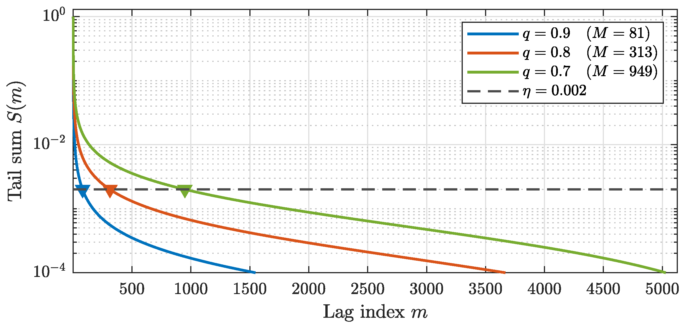
Truncating the convolution to a finite window of length M (Section 2.2) reduces the per-evaluation cost from $\mathcal{O}\left(n^2\right)$ to $\mathcal{O}\left(nM\right)$. At a fixed window $M=2000$, a single FO-Lorenz system evaluation falls to $6.4$ s, a reduction of roughly two orders of magnitude relative to full memory, and the step that makes the search tractable. We further set M adaptively for each candidate using the tail-sum criterion (8): because the GL weights decay faster as $q_i\to 1$ (Section 2.2), near-integer candidates require only a short window. The per-evaluation time falls to $3.4$ s at $q=1.0$, whereas a stronger fractional candidate ($q=0.7$) retains a longer window at $5.1$ s. The adaptive scheme thus reduces cost most where the kernel permits and preserves the longer memory where the dynamics require it, rather than imposing a uniform cut. Table 1 summarises the three regimes, their complexity, and their evaluation time.

Two further levers control cost. First, the truncation tolerance $\eta$ directly trades accuracy for speed: a larger $\eta$ yields a smaller M and a lower cost. The sensitivity study of Section 3.3 shows that tightening $\eta$ from $2\times {10}^{-3}$ to ${10}^{-3}$ shifts the optimized ${\lambda }_1$ by less than $0.4\%$ at roughly four times the wall-clock cost, so the chosen $\eta =2\times {10}^{-3}$ sits in a stable, favorable region of this trade-off. Second, the GL convolution is implemented as a vectorized weight-history product rather than an explicit per-lag loop, giving a constant-factor speedup. Finally, the per-iteration population evaluation has no within-iteration sequential dependence and parallelizes cleanly via parfor (Table 9).

On scalability, the per-evaluation cost grows with the truncated window M and with the size of the variational system ($n^2$ components for an n-dimensional system), while the decision-vector dimension grows linearly with system order ($d=2n$). The adaptive window and population-level parallelization together keep the four-system study tractable, with the largest case (nine-dimensional Hyper-Chen search) completing in ≈6 h on eight cores.

3.4. Results

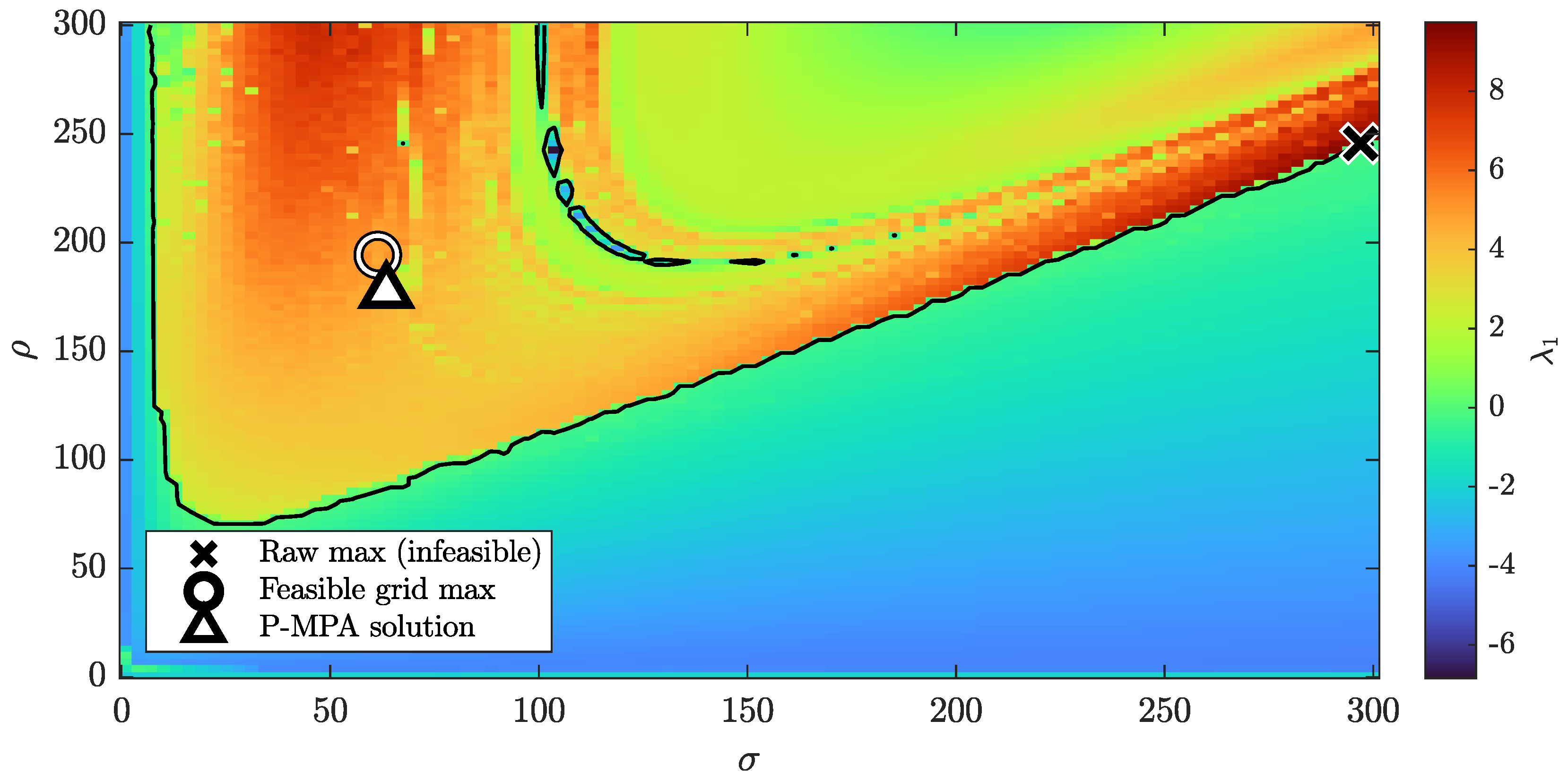
A two-parameter grid sweep was conducted in the $(\sigma ,\rho )$ plane with $\beta =4$ and $\mathbf{q}=(0.985,0.99,0.98)$ fixed at the values of [17]. A $100\times 100$ grid over $\sigma ,\rho \in [1,300]$ produced the ${\lambda }_1(\sigma ,\rho )$ map of Figure 2. The landscape is strongly non-convex and multimodal. This confirms that gradient-free search is necessary.

The unconstrained grid maximum is ${\lambda }_1=9.750$ at $\sigma =296.98$ and $\rho =245.64$. It is infeasible ($\mathcal{P}=856.18$) and violates simultaneous boundedness and chaotic signature. After restricting to feasible candidates, the grid maximum is ${\lambda }_1=4.746$ at $(\sigma ,\rho )=(61.40,194.29)$. The P-MPA solver with the penalized objective (17) and (18) converges to ${\lambda }_1^{*}=4.777$ at $({\sigma }^{*},{\rho }^{*})=(63.45,177.36)$ (Figure 2). The $0.65\%$ relative agreement (within one grid cell) confirms that the optimizer correctly navigates the feasible landscape. It is not pulled into the infeasible high-${\lambda }_1$ corner.

Ten independent P-MPA runs were executed for the full six-dimensional search using the configuration of Section 3.3 and the bounds of (16). The stored best positions were then evaluated through the same objective function used inside the optimization loop. The values reported in Table 2 correspond to these evaluations. All ten runs satisfy $\mathcal{P}=0$. This confirms that the penalty stack correctly retains bounded, dissipative solutions with the three-dimensional chaotic signature throughout the search.

The feasible global optimum is Run 1, with the following parameters:

$$({\sigma }^{*},{\rho }^{*},{\beta }^{*})=(13.6778,499.8036,18.3544),{\mathbf{q}}^{*}=(0.8971,0.9987,1.0000).$$

(20)

The Lyapunov spectrum is $({\lambda }_1^{*},{\lambda }_2^{*},{\lambda }_3^{*})=(27.076,0.0995,-80.052)$. The trace is ${\sum }_i{\lambda }_i^{*}=-52.877<0$, so the solution is strictly dissipative. The Kaplan–Yorke dimension is $D_{KY}=2.339$. The incommensurate order vector combines strong fractional memory in the x-channel ($q_1=0.897$) with near-integer dynamics in y and z ($q_2=0.999$, $q_3=1.000$). This is consistent with the established result that incommensurate fractional-order systems sustain chaos at parameter values inaccessible to their commensurate counterparts [14,17]. The optimum (20) places ${\rho }^{*}\approx 500$, far above the classical $\rho =28$. As per Section 3.1, this is read as a chaos-maximizing operating point of the governing equations, not as a physical regime.

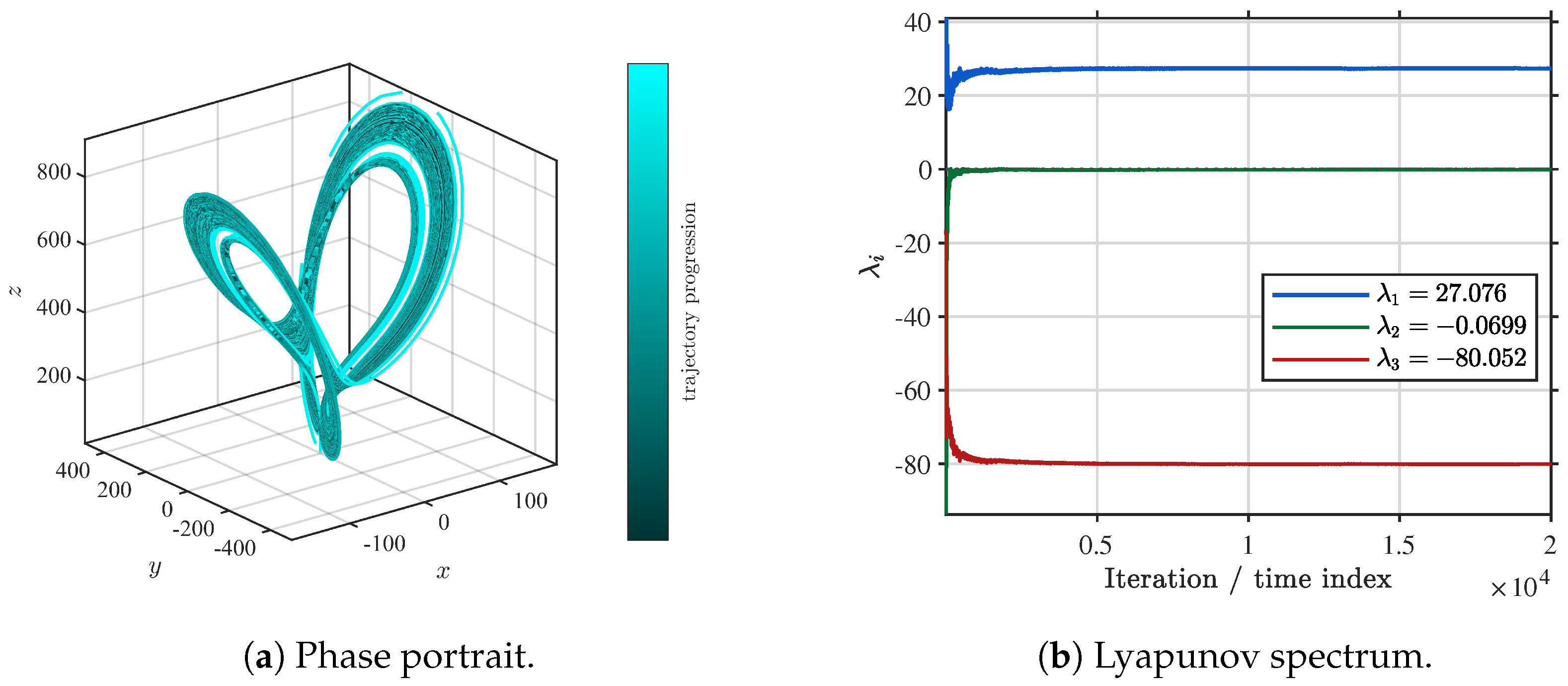
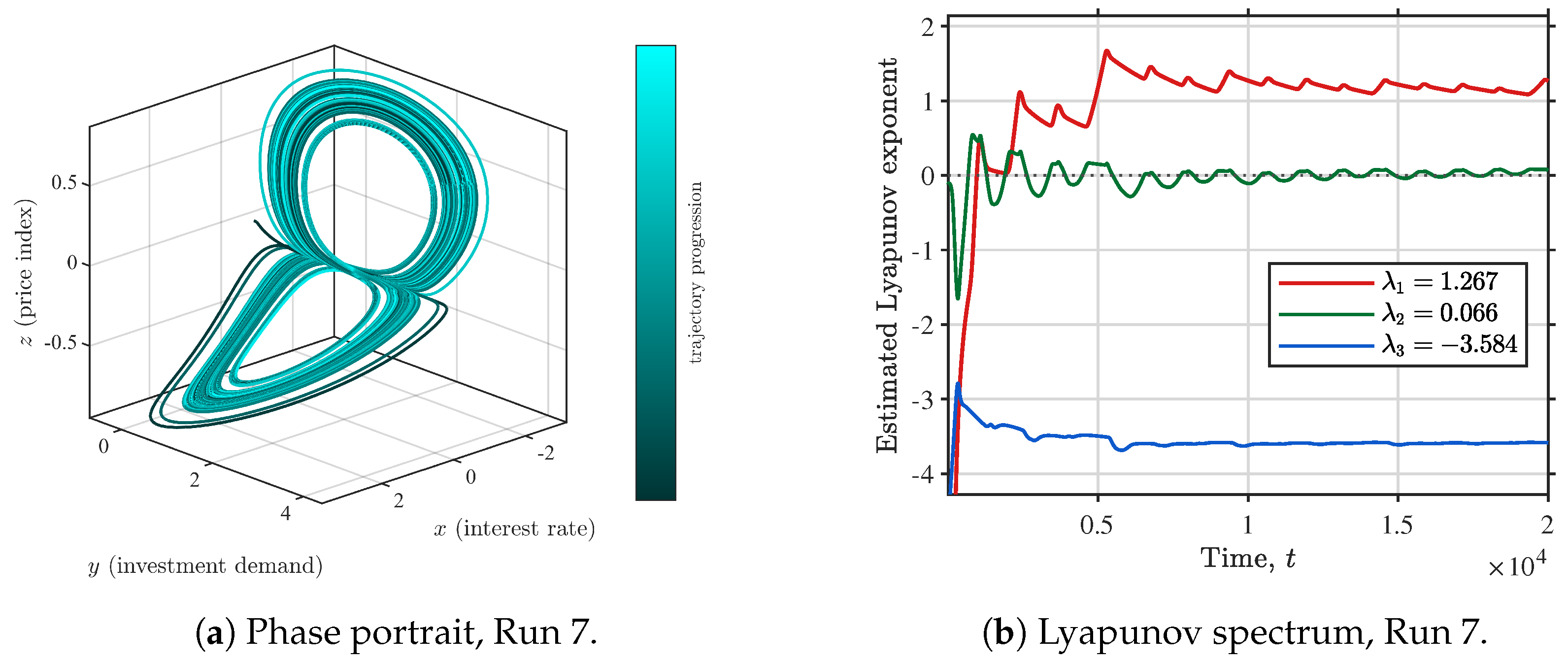
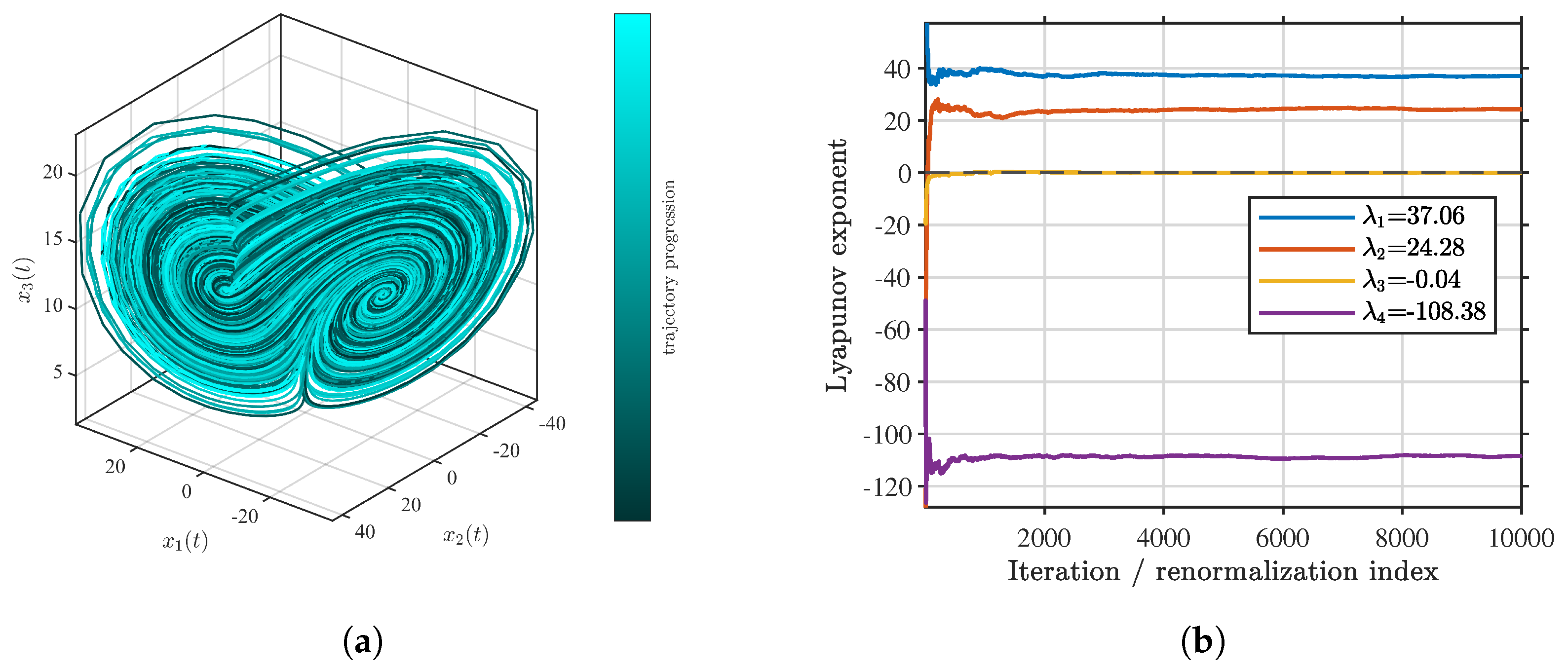
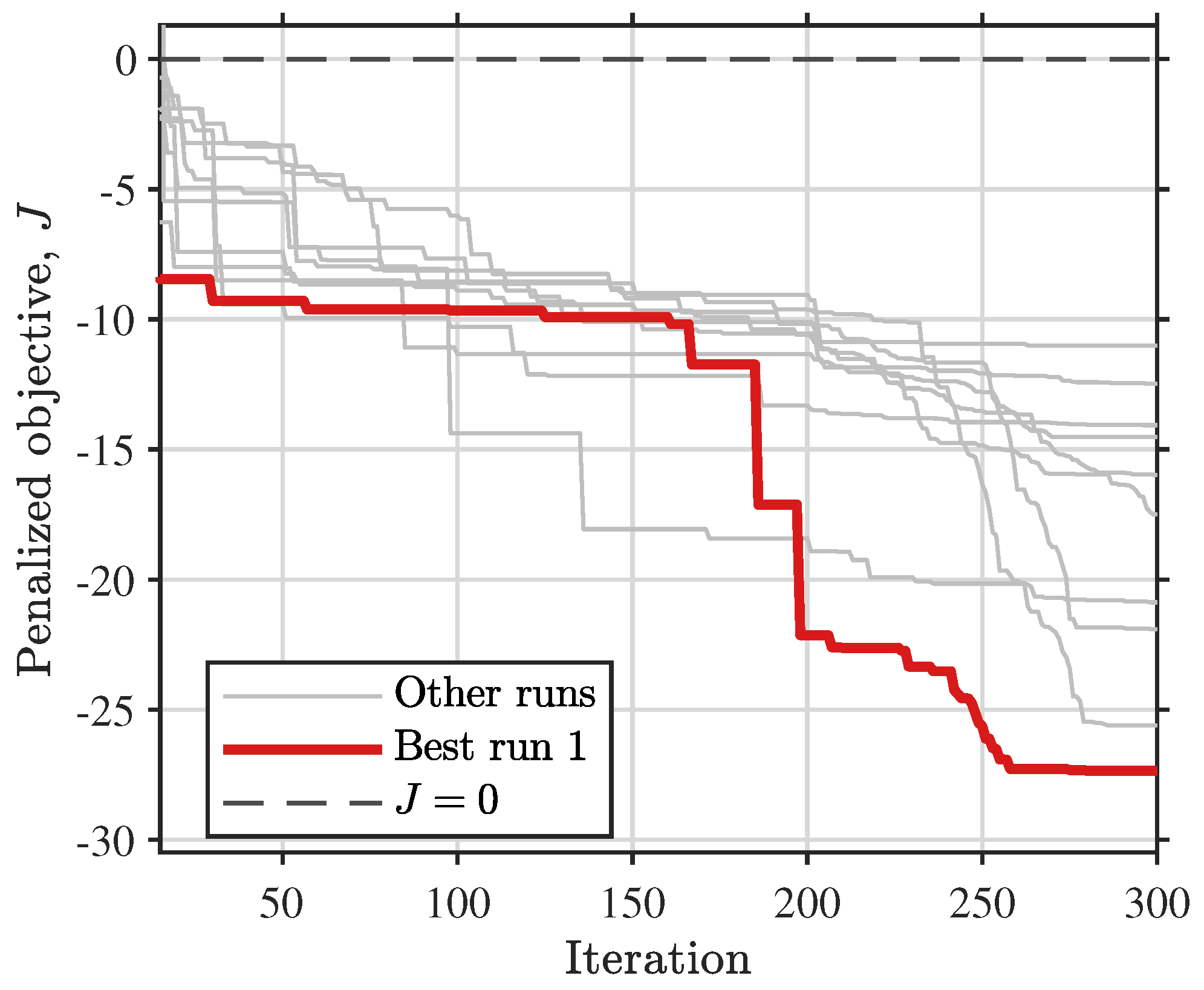
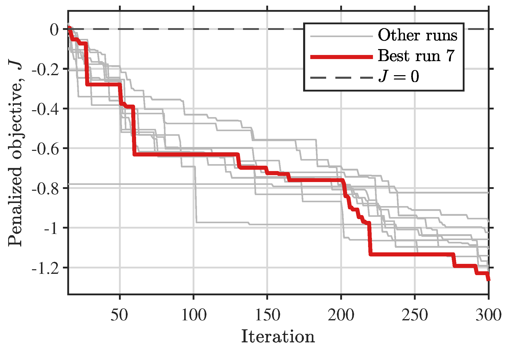
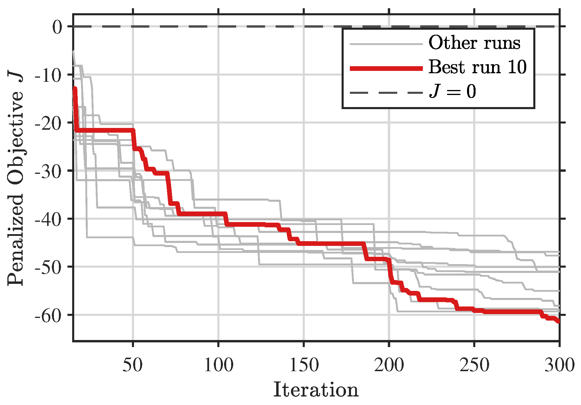
Figure 3 verifies the solution. The butterfly attractor is bounded, and the LE spectrum converges cleanly to its three asymptotic values. Figure 4 shows the convergence histories of the ten runs. Since all final penalties vanish, the objective enters the merit-only regime in which $J=-{\lambda }_1^{\left(f\right)}$. The best run is highlighted in red.

Table 3 contextualizes the present framework within prior Lorenz-family optimization studies. The comparison is deliberately framed around search space and feasibility treatment. It is not framed around absolute ${\lambda }_1$. As noted in the introduction, a wider upper bound on $\rho$ admits attractors of larger spatial extent and correspondingly larger exponential expansion rates. That alone does not constitute a methodological advance. The appropriate comparison is over the methodological framework, which is the objective of this paper.

The methodological contribution has four components, each operationalized in the present framework. First, the penalty design (17) and (18) encodes the necessary dynamical conditions as subtractive hinges that vanish on the feasible set. These conditions are dissipativity, boundedness, asymptotic stability of the LE estimate, and the dimension-appropriate chaotic signature. Once $\mathcal{P}=0$, the search operates purely on the merit term. Second, the inner loop uses the memory-consistent GL variational estimator of Li et al. [17], applied row by row. Third, the system parameters and incommensurate fractional orders are optimized jointly within a single six- to nine-dimensional decision vector. Fourth, the framework is system-agnostic. The same outer loop, inner-loop estimator, and penalty design are applied without modification across the four target systems. The only adjustment is one threshold replacement for the four-dimensional cases.

Prior optimization studies on chaotic systems differ from the present framework not only in the algorithm but also in the problem definition, which makes their reported results not directly comparable. Silva-Juárez et al. [21] maximized ${\lambda }_1$ of the integer-order Lorenz system over the parameters $(\sigma ,\rho ,\beta )$ only, reporting ${\lambda }_1=6.766$ at $\sigma \approx 60,\rho =180,\beta \approx 30$. Moreover, the feasibility was handled implicitly through eigenvalue-based step-size selection, with no explicit boundedness, dissipativity, or signature constraints. Sahoo et al. [22] maximized the Kaplan–Yorke dimension of the integer-order Lorenz system over parameters and initial conditions, obtaining ${\lambda }_1=7.914$ as a by-product ($D_{KY}=2.169$); their constraint treatment uses a quadratic penalty on ${({\lambda }_1-{\lambda }_1^{lim})}^2$ and ${({\lambda }_2-{\lambda }_2^{lim})}^2$, which remains active on the feasible set and so distorts the merit landscape, in contrast to the subtractive hinges used here. Adeyemi et al. [16] maximized the MLE of a fractional-order spherical system (not Lorenz) over eleven variables, including a single commensurate order, raising the MLE from $0.018$ to $1.081$. The inner loop used an integer-order Benettin–Wolf estimator, which can be biased in the strongly fractional regime, and the search does not expose incommensurate parameter-order coupling. Common to all three is that the order is integer or commensurate, the inner-loop estimator ignores the row-dependent Grünwald–Letnikov memory, and absolute ${\lambda }_1$ is reported under heterogeneous bounds. A summary of the aforementioned optimization studies is reported in Table 3.

To obtain a quantitative comparison, we isolate the effect of the optimizer by holding the system, objective, bounds, and inner-loop estimator fixed and varying only the outer-loop optimization algorithm. Three representative metaheuristics (differential evolution [21], particle swarm optimization, and a competitive-swarm-type optimizer (CSO)) are applied to the identical fractional-order Lorenz problem (15), penalized objective (17) and (18), search bounds (16), and memory-consistent GL inner-loop estimator of Section 2.3 used for P-MPA. All optimizers use equal population size, iteration count, and ten independent seeded trials. This comparison measures search capability on the proposed landscape, rather than the end-to-end pipelines of the cited studies. The results are reported in Table 4.

P-MPA attains the largest best, mean, and median ${\lambda }_1$. DE and PSO converge to a feasible solution but markedly lower optima; CSO is the least reliable, with both the lowest median and a single divergent run. Furthermore, while nine CSO trials remained feasible, one run diverged into the infeasible region ($\mathcal{P}>0$), which is consistent with its unclamped velocity update. On this non-convex, multimodal, gradient-free landscape with a two-phase (feasibility-then-merit) structure, the phase-based exploration of MPA (Brownian and Lévy movement with the FAD escape mechanism) appears to balance global exploration and local refinement more effectively on this problem than the selection of DE or the velocity-driven updates of PSO and CSO. The combination of search quality (Table 4) and parallel tractability motivates the use of the parallel P-MPA throughout this work.

4. Optimization Across Diverse Fractional-Order Chaotic Systems

The framework of Section 3 is now applied to three further systems. These are chosen to span a representative range of fractional chaos. The first is the Ma–Chen fractional-order financial system [28,29]. The second is the four-dimensional Iqbal–Wang hyperchaotic system recently introduced in [30]. The third is the four-dimensional Hyper-Chen hyperchaotic system [31]. The outer-loop optimizer, the inner-loop Lyapunov estimator, the numerical parameters $(h,\eta ,N_{QR})$, and the penalty multipliers are unchanged from Section 3.3. Only two system-specific modifications are required. The first is the calibrated value of the boundedness threshold ${\delta }_{\mathrm{th}}$, together with the system-specific search bounds. The threshold follows the rule ${\delta }_{\mathrm{th}}=\gamma {\delta }_{\mathrm{rel}}^{\mathrm{ref}}$, where ${\delta }_{\mathrm{rel}}^{\mathrm{ref}}$ is the relative deviation measured at the system’s canonical reference and $\gamma$ is a fixed margin chosen to admit enlarged but still physically bounded attractors. For the FO financial system at $(a,b,c)=(0.01,0.1,1.0)$ with $\mathbf{q}=(0.985,0.99,0.98)$ the reference is $0.0584$, and $\gamma =4$ yields ${\delta }_{\mathrm{th}}=0.2336$. For the FO Iqbal–Wang system at $(a_1,\dots ,a_5)=(30,1,0.4,3,19)$ with $\mathbf{q}=\mathbf{1}$ the reference is $0.5046$, and $\gamma =4$ yields ${\delta }_{\mathrm{th}}=2.0186$. For the FO Hyper-Chen system at $(a,b,c,d,k_a)=(36,3,28,-16,0.5)$ with $\mathbf{q}=\mathbf{0}.\mathbf{95}$ the reference is $1.6008$, and $\gamma =3$ yields ${\delta }_{\mathrm{th}}=4.8024$. The second applies to the two four-dimensional systems. In a four-dimensional hyperchaotic attractor, the expected signature is two positive exponents, one near-zero exponent, and one strongly negative exponent. The three-dimensional chaotic-signature hinge $p_{{\lambda }_2}$, which penalizes departures of ${\lambda }_2^{\left(f\right)}$ from zero, is therefore replaced by a hyperchaotic-signature hinge $p_{{\lambda }_3}$ on the third exponent:

$$p_{{\lambda }_3}=\left\{\begin{array}{cc}0,\hfill & \left|{\lambda }_3^{\left(f\right)}\right|<{ϵ}_{{\lambda }_3},\hfill \\ \left|{\lambda }_3^{\left(f\right)}\right|,\hfill & \mathrm{otherwise},\hfill \end{array}\right.{ϵ}_{{\lambda }_3}=0.15.$$

(21)

The merit term is also adjusted. Since the goal is to maximize the strength of both positive exponents simultaneously, the scalar objective minimized by the outer loop becomes

$$J\left(\mathit{\theta }\right)=B·\mathcal{P}\left(\mathit{\theta }\right)-\left({\lambda }_1^{\left(f\right)}+{\lambda }_2^{\left(f\right)}\right),\mathcal{P}=p_{\mathrm{sum}}+p_{\mathrm{bnd}}+p_{\mathrm{std}}+p_{{\lambda }_3},B={10}^2.$$

(22)

Together, these two changes constrain the optimizer to retain genuine hyperchaos throughout the search, while penalizing solutions in which the third exponent drifts away from zero.

4.1. Fractional-Order Financial System (Ma–Chen)

The Ma–Chen finance model [28,29] couples interest rate x, investment demand y, and price index z through $\dot{x}=z+(y-a)x$, $\dot{y}=1-by-x^2$, $\dot{z}=-x-cz$. Here $a\ge 0$ represents the savings amount, $b\ge 0$ represents the cost per investment, and $c\ge 0$ represents the elasticity of demand. The fractional-order extension of Chen [40] is motivated by the long-memory character of financial time series [41]:

$${}_0{}^{\mathrm{GL}}{D}_t^{q_1}x=z+(y-a)x,{}_0{}^{\mathrm{GL}}{D}_t^{q_2}y=1-by-x^2,{}_0{}^{\mathrm{GL}}{D}_t^{q_3}z=-x-cz,$$

(23)

with $\mathbf{q}=(q_1,q_2,q_3)\in (0,1]$. At the standard chaotic regime $(a,b,c)=(0.01,0.1,1.0)$ and $\mathbf{q}=(0.985,0.99,0.98)$ [40,42], the Lyapunov spectrum is approximately $(0.087,0,-1.06)$ with $D_{KY}\approx 2.082$.

The decision vector is $\mathit{\theta }=[a,b,c,q_1,q_2,q_3]$, where the boxed constraints are $a\in [0.005,2.0]$, $b\in [0.1,1.0]$, $c\in [0.5,5.0]$, and $q_i\in [0.7,1.0]$. The bounds on a and c are widened relative to the canonical regime, so that the search is not artificially confined to a small neighborhood of $(0.01,0.1,1.0)$. The calibrated boundedness threshold ${\delta }_{\mathrm{th}}=0.2336$ reflects the much smaller spatial extent of the financial attractor relative to the Lorenz system.

Table 5 lists the ten independent P-MPA runs. All ten runs satisfy $\mathcal{P}=0$. The feasible global optimum is Run 7, with $(a^{*},b^{*},c^{*})=(0.4880,0.1030,3.0173)$ and ${\mathbf{q}}^{*}=(0.8349,1.0000,0.9727)$. The Lyapunov spectrum is $(+1.2670,+0.0663,-3.5842)$, the trace is $-2.2509$, and $D_{KY}=2.3720$. The trace is strictly negative, so the optimum corresponds to a bounded dissipative strange attractor. Figure 5 shows the phase portrait and LE spectrum of Run 7, while Figure 6 shows the ten convergence histories.

4.2. Fractional-Order Iqbal–Wang Four-Dimensional Hyperchaotic System

Iqbal and Wang [30] recently introduced a four-dimensional hyperchaotic system. It has two nonlinear terms ($xw$ and $-xz$) and bidirectional x–y coupling. Replacing the integer-order derivatives by GL fractional derivatives of incommensurate orders gives

$$\begin{array}{cc}\hfill {}_0{}^{\mathrm{GL}}{D}_t^{q_1}x& =a_1(w-x)+a_{2}y,\hfill \\ \hfill {}_0{}^{\mathrm{GL}}{D}_t^{q_2}y& =w-a_{3}x,\hfill \\ \hfill {}_0{}^{\mathrm{GL}}{D}_t^{q_3}z& =xw-a_{4}z,\hfill \\ \hfill {}_0{}^{\mathrm{GL}}{D}_t^{q_4}w& =-xz+a_{5}w.\hfill \end{array}$$

(24)

At the canonical regime $(a_1,\dots ,a_5)=(30,1,0.4,3,19)$ and integer order, Iqbal and Wang report the Lyapunov spectrum $(2.0393,0.0216,-0.0007,-16.0602)$ with $D_{KY}=3.1283$. At commensurate fractional order $\alpha =0.98$, they report $(2.1747,0.0190,-0.0003,-17.3006)$ with $D_{KY}=3.1268$ [30]. Using our GL variational estimator, we recovered $(2.039,0.024,-0.001,-16.062)$ and $(2.175,0.019,-0.000,-17.301)$, respectively. The relative disagreement in ${\lambda }_1$ is below $0.5\%$ in both cases.

The decision vector is the nine-dimensional vector $\mathit{\theta }=[a_1,a_2,a_3,a_4,a_5,q_1,q_2,q_3,q_4]$. Following the optimization script, the search domain was defined as $a_1\in [0.5,50]$, $a_2\in [0.01,10]$, $a_3\in [0.1,10]$, $a_4\in [0.1,30]$, $a_5\in [0.1,50]$, and $q_i\in [0.9,1.0]$ for $i=1,\dots ,4$. The population size was $N_{\mathrm{pop}}=63$, and the merit term was ${\lambda }_1+{\lambda }_2$. Table 6 lists the ten independent P-MPA runs after optimization, where all runs satisfy the implemented hinges ($\mathcal{P}=0$, with $p_{{\lambda }_3}$ substituted for $p_{{\lambda }_2}$), and every run also satisfies the strict hyperchaos condition ${\lambda }_2>0$.

The best-merit solution is obtained in Run 5, with a merit value ${\lambda }_1+{\lambda }_2=15.0116$ and a Kaplan–Yorke dimension $D_{\mathrm{KY}}=3.3837$. The Lyapunov trace satisfies ${\sum }_i{\lambda }_i=-24.1651<0$, indicating that the optimum is strictly dissipative. Compared to the integer-order canonical baseline ${\lambda }_1=2.0393$, the best-merit solution increases the largest Lyapunov exponent by approximately $4.21\times$, while relative to the commensurate fractional baseline ${\lambda }_1=2.1747$, the increase is approximately $3.95\times$.

Figure 7 shows the $(x,y,w)$-projection of the best hyperchaotic attractor (Run 5) and its full Lyapunov spectrum, while Figure 8 shows the ten convergence histories.

4.3. Fractional-Order Hyper-Chen System

The Hyper-Chen system adds a linear feedback channel to the Chen attractor, producing four-dimensional hyperchaos [43]. Its fractional-order form [31] is

$$\begin{array}{cc}\hfill {}_0{}^{\mathrm{GL}}{D}_t^{q_1}{x}_1& =a(x_2-x_1),\hfill \\ \hfill {}_0{}^{\mathrm{GL}}{D}_t^{q_2}{x}_2& =d{x}_1-x_1{x}_3+c{x}_2-x_4,\hfill \\ \hfill {}_0{}^{\mathrm{GL}}{D}_t^{q_3}{x}_3& =x_1{x}_2-b{x}_3,\hfill \\ \hfill {}_0{}^{\mathrm{GL}}{D}_t^{q_4}{x}_4& =x_1+k_a,\hfill \end{array}$$

(25)

with a nine-dimensional decision vector $\mathit{\theta }=[a,b,c,d,k_a,q_1,q_2,q_3,q_4]$. At the canonical regime $(a,b,c,d,k_a)=(36,3,28,-16,0.5)$ and $\mathbf{q}=(0.95,0.95,0.95,0.95)$, the integer-order Hyper-Chen attractor admits two positive Lyapunov exponents ${\lambda }_1\approx 1.55$ and ${\lambda }_2\approx 0.16$, with $D_{KY}\approx 3.08$ [43].

The optimization boxed bounds are $a\in [10,100]$, $b\in [2,20]$, $c\in [10,100]$, $d\in [-50,-5]$, $k_a\in [0.1,1.0]$, and $q_i\in [0.7,1.0]$. The three-dimensional signature hinge is again replaced by the hyperchaos hinge of (21) and (22). The population size is $N_{\mathrm{pop}}=63$. Table 7 lists the optimization results of the ten independent runs, where all runs are feasible with $\mathcal{P}=0$. The best-merit solution is Run 10, with merit ${\lambda }_1+{\lambda }_2=61.3402$ and $D_{KY}=3.5656$. The trace of the Lyapunov spectrum at Run 10 is ${\sum }_i{\lambda }_i=-47.0769<0$, so the optimum is strictly dissipative. It also preserves the hyperchaos signature: the first two Lyapunov exponents are strongly positive, the third is near zero, and the fourth is strongly negative. Figure 9 shows the $(x_1,x_2,x_3)$-projection of the optimized hyperchaotic attractor and its LE spectrum, while Figure 10 shows the ten convergence histories, with Run 10 highlighted.

4.4. Cross-System Signature

Table 8 consolidates the cross-system picture. Under a single fixed configuration, the framework converges, on each of the four systems, to feasible attractors with substantially enlarged dominant Lyapunov exponents relative to their canonical regimes. All four optima are strictly dissipative: the ${\sum }_i{\lambda }_i$ column of Table 8 is negative in every row. Across all systems, the Kaplan–Yorke dimension is at or above the canonical baseline, and the hyperchaos signature is preserved in both four-dimensional cases.

Table 9 reports the wall-clock cost of producing each row of Table 8, so that every result above can be reproduced under a stated budget. The control settings are identical across systems: the population is fixed at $N_{\mathrm{pop}}=7d$ and the search runs for a fixed 300 iterations, giving $n_{\mathrm{eval}}=300N_{\mathrm{pop}}=2100d$ objective evaluations per run. The dimension d is thus the only quantity that varies, and it drives both the population size and the total number of evaluations.

5. Synchronization Analysis and Application Demonstration

Section 3 and Section 4 have established that the P-MPA framework produces attractors with enlarged Lyapunov spectra and Kaplan–Yorke dimension across the systems studied. The framework uses a memory-consistent GL variational LE estimator and subtractive feasibility hinges. We next examine whether the upstream dynamical gains translate into a measurable difference downstream. We address this question along two complementary lines. First, we examine a quantity of intrinsic interest in nonlinear dynamics: the synchronization threshold of a coupled response system. This is addressed in Section 5.1 through a fractional conditional Lyapunov exponent (FCLE) analysis. Second, we examine the output stage of a representative downstream application. This is addressed in Section 5.2 through a compact demonstration based on a chaos-based pseudo-random number generator (PRNG) and an image-encryption pipeline.

The cipher and its keystream are assessed using the standard empirical battery of the chaos-based encryption literature [3]: the NIST SP 800-22 Rev. 1a randomness suite [44]; byte entropy; adjacent-pixel correlation in the horizontal, vertical, and diagonal directions; the differential metrics NPCR and UACI; and the histogram-uniformity ${\chi }^2$ test. These benchmarks evidence the absence of detectable statistical structure in the keystream and the cipher output at the resolution of the tests; consistent with the framing of this section, they are not advanced as a formal cryptographic security analysis. All NIST SP 800-22 p-values were computed with the open-source Python 3.13 implementation of Johnston [45] at its default block-length parameters and significance level $\alpha =0.01$.

5.1. Fractional Conditional Lyapunov Exponent (FCLE)

A common claim in the chaos-synchronization literature is that a larger dominant Lyapunov exponent ${\lambda }_1$ increases the coupling gain required for observer-based drive–response synchronization. In the integer-order setting, this is made precise by full-state diffusive (proportional-feedback) coupling: two identical systems coupled on every state synchronize when the gain exceeds the maximal Lyapunov exponent, so that $c_{min}^{IO}={\lambda }_1$. This identity originates with Fujisaka and Yamada [46], underlies the master-stability-function formulation of Pecora and Carroll [47], and was established rigorously for a broad class of systems by Baumann and Leine [48], who use the critical coupling to estimate ${\lambda }_{max}$. We adopt full-state coupling as the primary construction: it provides a clean analytical baseline against which the GL estimator can be validated, after which we examine how the threshold behaves under incommensurate fractional memory and under the more restrictive single-state coupling used in many chaos-based pipelines.

For the FO-Lorenz system in a drive–response configuration, the full-state coupled response is

$${}_0{}^{\mathrm{GL}}{D}_t^{q_1}{x}_r=\sigma (y_r-x_r)+c(x_d-x_r),{}_0{}^{\mathrm{GL}}{D}_t^{q_2}{y}_r=x_r(\rho -z_r)-y_r+c(y_d-y_r),{}_0{}^{\mathrm{GL}}{D}_t^{q_3}{z}_r=x_r{y}_r-\beta z_r+c(z_d-z_r),$$

(26)

with drive states $(x_d,y_d,z_d)$ and gain $c\ge 0$. Writing the synchronization error $\mathbf{e}=(x_d-x_r,$ $y_d-y_r,z_d-z_r{)}^T$ and linearizing about $\mathbf{e}=\mathbf{0}$ gives the error system:

$$\left(\begin{array}{c}{}_0{}^{\mathrm{GL}}{D}_t^{q_1}{e}_1\\ {}_0{}^{\mathrm{GL}}{D}_t^{q_2}{e}_2\\ {}_0{}^{\mathrm{GL}}{D}_t^{q_3}{e}_3\end{array}\right)=\left[\mathbf{A}\left(t\right)-c\mathbf{I}\right]\mathbf{e},\mathbf{A}\left(t\right)=\left[\begin{array}{ccc}-\sigma & \sigma & 0\\ \rho -z_d\left(t\right)& -1& -x_d\left(t\right)\\ y_d\left(t\right)& x_d\left(t\right)& -\beta \end{array}\right],$$

(27)

in which the coupling enters as $-c\mathbf{I}$. Applying the GL tangent-map construction of Section 2.3 row by row to the error Jacobian ${\mathbf{J}}^{\mathrm{err}}(t,c)=\mathbf{A}\left(t\right)-c\mathbf{I}$, the deviation matrix evolves as

$$A_{i,:}^{(k+1)}=h^{q_i}{\mathbf{J}}_{i,:}^{\mathrm{err}}\left(t_k\right){\mathbf{A}}^{\left(k\right)}-{\displaystyle \sum _{r=1}^{min(k,M)}}{w}_r^{\left(q_i\right)}{A}_{i,:}^{(k+1-r)},i=1,2,3,$$

(28)

and the FCLE is the largest transverse exponent,

$${\Lambda }_{\mathrm{FCLE}}\left(c\right)=\underset{K\to \infty }{lim}{\displaystyle \frac{1}{K{N}_{QR}h}}{\displaystyle \sum _{\kappa =1}^K}\ln \parallel {\mathbf{v}}_1^{\left(\kappa \right)}\parallel ,$$

(29)

where ${\mathbf{v}}_1^{\left(\kappa \right)}$ the first Gram–Schmidt vector at the $\kappa$-th re-orthonormalization. The pair synchronizes permanently once ${\Lambda }_{\mathrm{FCLE}}\left(c\right)<0$.

At $q_i=1$ the row-specific memory terms in (28) collapse to a single shared kernel, and the error system reduces to $\dot{\mathbf{e}}=[\mathbf{A}\left(t\right)-c\mathbf{I}]\mathbf{e}$, whose conditional exponents are exactly $\{{\lambda }_i-c\}$. The FCLE is then the straight line ${\lambda }_1-c$, crossing zero at $c={\lambda }_1$. The GL estimator reproduces this: at the canonical parameters, it returns ${\lambda }_1=0.715$ and a zero crossing at $c_{min}=0.715$, and the computed curve lies on the analytical line over the whole range (Figure 11a). It is worth noting that the value ${\lambda }_1=0.715$ at $h=5\times {10}^{-4}$ is affected by the first-order discretization used in the GL scheme; refining h moves both ${\lambda }_1$ and the crossing toward the textbook ${\lambda }_1\approx 0.906$ without affecting their coincidence. This recovers the Fujisaka–Yamada/Baumann–Leine identity $c_{min}^{IO}={\lambda }_1$ and validates the estimator in the integer-order limit before it is applied to the fractional regime.

For the optimized FO-Lorenz system (Run 1, ${\lambda }_1=27.076$) under full-state coupling, the FCLE remains monotone in c and crosses zero at $c_{min}^{FO}=24.5\approx 0.90{\lambda }_1$ (Figure 11b). The threshold sits just below ${\lambda }_1$: the fractional memory and the state-dependent cross-terms together act, on balance, to assist synchronization, and full-state synchronization of the optimized attractor is achieved at a gain on the order of ${\lambda }_1$, as the integer-order theory predicts.

Many chaos-based pipelines transmit a single scalar signal, corresponding to coupling only the x-channel,

$${}_0{}^{\mathrm{GL}}{D}_t^{q_1}{x}_r=\sigma (y_r-x_r)+c(x_d-x_r),{}_0{}^{\mathrm{GL}}{D}_t^{q_2}{y}_r=x_r(\rho -z_r)-y_r,{}_0{}^{\mathrm{GL}}{D}_t^{q_3}{z}_r=x_r{y}_r-\beta z_r,$$

(30)

for which the error system becomes $\dot{\mathbf{e}}=[\mathbf{A}\left(t\right)-\mathrm{diag}(c,0,0)]\mathbf{e}$. Here the gain damps $e_1$ directly, but the errors $e_2,e_3$ are driven by the state-dependent off-diagonal entries ${\mathbf{A}}_{21}=\rho -z_d\left(t\right)$ and ${\mathbf{A}}_{32}=x_d\left(t\right)$, which are not directly damped by the coupling. Single-state coupling is therefore substantially more demanding. Already at integer order the threshold is $c_{min}=6.0\approx 8{\lambda }_1$ (Figure 11c), far above the full-state value. For the optimized FO-Lorenz system it rises to $c_{min}^{FO}=243\approx 9{\lambda }_1$ (Figure 11d). Both profiles are monotone, so the binding constraint is the coupling topology (one channel versus three) rather than a fractional-order instability.

Two observations are seen from

Table 10. FCLE synchronization thresholds: Full-state versus single-state (x-coupling), integer-order and optimized FO-Lorenz system.

	Full-State (Primary)		x-Only (Single-State)
Metric	Integer (${\mathit{q}}_{\mathit{i}}=\mathbf{1}$)	Optimized	Integer (${\mathit{q}}_{\mathit{i}}=\mathbf{1}$)	Optimized
${\lambda }_1$	$0.715$	$27.076$	$0.715$	$27.076$
$c_{min}$	$0.715$	$24.5$	$6.0$	243
$c_{min}/{\lambda }_1$	$1.01$	$0.90$	$8.03$	$9.0$
${\Lambda }_{\mathrm{FCLE}}\left(c\right)$ profile	line, slope $-1$	monotone	monotone	monotone

. First, under full-state coupling, the synchronization threshold tracks ${\lambda }_1$ as the Fujisaka–Yamada/Baumann–Leine theory predicts: exactly at integer order ($c_{min}={\lambda }_1$, the validation) and to within $10\%$ for the fractional optimized attractor ($c_{min}\approx 0.90{\lambda }_1$). Second, single-state coupling raises the threshold by nearly an order of magnitude ($c_{min}\approx 8$–$9{\lambda }_1$), a gap set by the attractor’s cross-terms rather than by the fractional memory. The enlarged ${\lambda }_1$ of the optimized attractor thus maps to a proportionally larger gain requirement, most pronounced for the single-channel coupling relevant to applications.

5.2. Application Demonstration: PRNG and Image Encryption

This subsection investigates the optimized fractional-order Lorenz attractor of Run 1, the configuration that maximizes the dominant Lyapunov exponent, as the entropy source of a chaos-based image-encryption pipeline adapted from the permutation–diffusion scheme of Zhu et al. [49]. The adopted metrics constitute the standard empirical assessment battery commonly used in the chaos-based encryption literature and are reported to position the demonstration within this established performance envelope. The pipeline is presented as an application of the optimized chaotic attractor, while the scope and limitations of the resulting statistical claims are discussed explicitly in Section 6.

The optimized fractional-order Lorenz system is integrated from the Run 1 parameters of (20) using the same Grünwald–Letnikov scheme, step $h=5\times {10}^{-4}$, and adaptive memory window (8) (tolerance $\eta =2\times {10}^{-3}$) employed in the dynamical analysis, so that the entropy source and the analyzed attractor are identical. After a transient of $N_{\mathrm{trans}}=5\times {10}^3$ samples is discarded, the three state variables are mapped to a single byte stream by 32-bit min–max normalization followed by a bitwise XOR combination:

$$\tilde{v}\left(n\right)=⌊{\displaystyle \frac{v\left(n\right)-v_{min}}{v_{max}-v_{min}}}(2^{32}-1)⌋,v\in \{x,y,z\},K\left(n\right)=\left(\tilde{x}\left(n\right)\oplus \tilde{y}\left(n\right)\oplus \tilde{z}\left(n\right)\right)\mathrm{mod}256.$$

(31)

A leading segment of ${10}^6$ bytes ($8\times {10}^6$ bits) is reserved for the randomness tests. Evaluated with the NIST SP 800-22 Rev. 1a suite at significance level $\alpha =0.01$, this segment passes all 15 tests shown in

Table 11. NIST SP 800-22 Rev. 1a results for the PRNG output.

No.	Test Name	p-Value	Result
1	Frequency (monobit)	0.4109	Pass
2	Frequency within block	0.0953	Pass
3	Runs	0.1007	Pass
4	Longest run of ones	0.3148	Pass
5	Binary matrix rank	0.6498	Pass
6	Discrete Fourier transform	0.0630	Pass
7	Non-overlapping template	0.9999	Pass
8	Overlapping template	0.8675	Pass
9	Universal statistical (Maurer)	0.2279	Pass
10	Linear complexity	0.7131	Pass
11	Serial	0.5174	Pass
12	Approximate entropy	0.5178	Pass
13	Cumulative sums	0.4286	Pass
14	Random excursions	0.1871	Pass
15	Random excursions variant	0.1465	Pass
	Tests Passed	15/15

.

To make the selected keystream segment image-dependent, a plaintext-dependent offset is computed from two weighted byte sums of the plaintext $\mathbf{p}=(p_1,\dots ,p_n)$, following the principle introduced by Zhu et al. [49]:

$$h_1=\left({\displaystyle \sum _{i=1}^n}{p}_i\left(i\mathrm{mod}257\right)\right)\mathrm{mod}65521,h_2=\left({\displaystyle \sum _{i=1}^n}{p}_i\left((n+1-i)\mathrm{mod}257\right)\right)\mathrm{mod}65521,\delta =(h_1·65521+h_2)\mathrm{mod}\Delta ,$$

(32)

with $\Delta =5\times {10}^5$. The offset $\delta$ selects, immediately after the reserved randomness segment, the confusion sub-stream ${\mathbf{k}}_1$ and the diffusion sub-stream ${\mathbf{k}}_2$; a single-pixel change in the plaintext alters $\delta$ and therefore both sub-streams. This is a lightweight operational device appropriate to the demonstration; it is not advanced as a defense against an adaptive chosen-plaintext adversary.

The cipher follows the classical permutation–diffusion template: an argsort permutation driven by ${\mathbf{k}}_1$ scrambles the pixel order, and a chained modular addition driven by ${\mathbf{k}}_2$ diffuses the result:

$${\mathbf{p}}_{\pi }=\mathbf{p}\left[\mathrm{argsort}\left({\mathbf{k}}_1\right)\right],C\left(i\right)=\left(C(i-1)+p_{\pi }\left(i\right)+k_2\left(i\right)\right)\mathrm{mod}256,C\left(0\right)=0,$$

(33)

with exact inverse $p_{\pi }\left(i\right)=(C\left(i\right)-C(i-1)-k_2\left(i\right))\mathrm{mod}256$. The scheme was evaluated on three standard test images: Cameraman at $256\times 256$ and Baboon and Peppers at $512\times 512$. As shown in Figure 12, the cipher images carry no visible structure, and lossless decryption with zero pixel error was confirmed on every image before any metric was computed.

Table 12. Empirical metrics of the application demonstration, averaged per image across color channels. Corr. H/V/D are the horizontal, vertical, and diagonal adjacent-pixel correlation coefficients. Ideal values are the theoretical references for an 8-bit cipher.

Image	Entropy	Corr. H	Corr. V	Corr. D	NPCR (%)	UACI (%)	${\mathit{\chi }}^2$ Pass
Cameraman ${256}^2$	7.9974	$+0.0028$	$-0.0206$	$-0.0078$	99.600	33.481	3/3
Baboon ${512}^2$	7.9992	$+0.0059$	$+0.0022$	$-0.0059$	99.608	33.457	2/3
Peppers ${512}^2$	7.9993	$-0.0043$	$+0.0003$	$+0.0076$	99.610	33.469	3/3
Theoretical ideal	8.0000	0	0	0	99.6094	33.4635	—

summarizes the cipher statistics averaged over the color channels of each image. The per-image mean cipher entropy ranges from $7.9974$ to $7.9993$ bits/pixel, remaining within $3\times {10}^{-3}$ of the ideal value of 8 bits/pixel. The channel-averaged adjacent-pixel correlation coefficients remain close to zero (all $\left|·\right|<0.021$) in the horizontal, vertical, and diagonal directions, against values near $0.95$ for the corresponding plaintexts, confirming effective suppression of first-order spatial redundancy. The average NPCR and UACI values fall within $99.600$–$99.610\%$ and $33.46$–$33.48\%$, respectively, in close agreement with the theoretical single-pixel-change ideals of $99.6094\%$ and $33.4635\%$ [50]. The histogram-uniformity ${\chi }^2$ test, using the critical value $293.25$ for 255 degrees of freedom at $\alpha =0.05$, is passed by eight of the nine color channels; the only failed case is the Baboon red channel, with ${\chi }^2=312.3$, which is consistent with the pronounced red-channel saturation in the original image and is reported transparently as an observed exception. The statistical effect of the cipher is illustrated for a representative image (Baboon) as an example in Figure 13, where the flattened cipher histograms and the diffuse cipher correlation clouds confirm the suppression of first- and second-order image structure.

These values place the demonstration within the statistical envelope reported in recent fractional-order chaos-based encryption studies that use related permutation–diffusion or semi-tensor-product constructions [8,49,51]. The contribution of the demonstration is not the envelope itself, which is common to many schemes, but its source; the keystream is generated from a dynamically optimized attractor rather than from a hand-tuned one.

6. Conclusions

This paper presented a constraint-faithful, reproducible optimization framework for incommensurate fractional-order chaotic and hyperchaotic systems. The framework combines four ingredients. First, the Penalized Marine Predators Algorithm uses subtractive hinges that vanish on the threshold-defined feasible set. Second, a memory-consistent Grünwald–Letnikov variational Lyapunov estimator with adaptive tail-sum truncation drives the inner loop. Third, the system parameters and incommensurate fractional orders $\mathbf{q}=(q_1,\dots ,q_n)$ are searched jointly in a single decision vector. Fourth, a fractional conditional Lyapunov exponent (FCLE) is defined, which reduces to the integer-order variational equation in the $q_i\to 1$ limit and recovers the threshold $c_{min}^{IO}={\lambda }_1$ as a special case.

The framework was applied without algorithmic modification, under a single fixed configuration, to four systems: the fractional-order Lorenz system (FO-Lorenz system), the Ma–Chen financial system, the four-dimensional Iqbal–Wang hyperchaotic system, and the Hyper-Chen system. On each system, the framework converged to feasible attractors with enlarged Lyapunov spectra and Kaplan–Yorke dimensions relative to the canonical regimes. The reported optima for all four systems satisfied ${\sum }_i{\lambda }_i<0$ at the reported precision, confirming strict dissipativity of the selected solutions. All Lyapunov claims in this work are numerical rather than analytical. They are stable to refinement of the GL parameters within the reported precision.

The FCLE was validated against the integer-order identity $c_{min}={\lambda }_1$ of Fujisaka–Yamada [46] and Baumann–Leine [48], which the GL estimator reproduces in the $q_i\to 1$ limit under full-state coupling ($c_{min}=0.724$ against ${\lambda }_1=0.715$). On the optimized FO-Lorenz system attractor, full-state synchronization occurs at $c_{min}\approx 0.90{\lambda }_1$, while single-state x-coupling raises the threshold to ≈9${\lambda }_1$. The synchronization threshold is therefore governed primarily by the coupling topology, and the enlarged ${\lambda }_1$ of the optimized attractor maps to a proportionally larger gain requirement.

The application demonstration, framed as empirical output validation rather than cryptanalysis, passed all 15 NIST SP 800-22 Rev. 1a tests at $\alpha =0.01$ on an $8\times {10}^6$-bit keystream. The remaining output metrics, byte entropy, adjacent-pixel correlation, and the differential measures NPCR and UACI, fall within the empirical envelope reported in the chaos-based encryption literature (Section 5.2), with a single histogram-uniformity ${\chi }^2$ exception on the Baboon red channel that is consistent with the pronounced red-channel saturation of that image. These results constitute a proof-of-concept demonstration of output quality rather than a formal security evaluation: they establish the absence of detectable statistical structure in the keystream and cipher output at the resolution of those tests, but do not constitute a cryptographic security proof. No resistance to chosen-plaintext, differential, algebraic, or side-channel attack is claimed or implied, and the lightweight plaintext-dependent keying of Section 5.2 is not advanced as a defense against an adaptive adversary. The sole purpose of the demonstration is to confirm that the dynamical gains delivered by the optimization framework persist at the output of a concrete downstream pipeline; a formal cryptanalytic evaluation lies outside the present scope and is identified as future work.

Several natural extensions follow. The first is the development of a higher-order or adaptive fractional integrator for the strongly fractional regime. The second is a dissipativity hinge based on the time-averaged divergence $\langle \nabla ·f\rangle$ for systems where local divergence is parameter-independent. The third is a formal cryptanalytic evaluation of the application pipeline. Additional validation directions are also natural. First, the predicted thresholds could be validated by direct drive–response integration of the coupled fractional system, measuring the synchronization error as a function of c and comparing the empirical critical coupling with the FCLE prediction. Second, the analysis could be extended to the other single-state configurations of Pecora and Carroll [27] (y- and z-drive) and to the master-stability-function formalism [47] for networks of coupled fractional oscillators. Third, a hardware (e.g., FPGA) realization of the optimized FO-Lorenz system attractor would test whether the elevated threshold persists under quantization and noise.