


Abstract
Alzheimer’s disease (AD) is a major type of cognitive impairment. Most existing studies on cognitive state classification focus on the direct application of various machine learning (ML) algorithms. These studies typically assume consistency in patient features across assessments, without explicitly accounting for the variability introduced by subjective evaluation. While a limited number of studies have attempted to address such variability, their applicability remains constrained. This study addresses the identified gap by proposing a distribution–coherent data refinement method. First, it incorporates SHAP-based feature selection, then excludes a subset of distributionally atypical records. These include records from patients with a single visit that contribute to increased intra-class variance and reduced inter-class separability, as well as records from patients with multiple visits that exhibit inconsistent longitudinal trajectories. The method operates on the training data, and the resulting refined training data is fed to ML algorithms. The experimental results show that detecting a small number of records (1.285%) leads to a minor enhancement in data quality. The Fisher score and Cohen’s f are increased by on average 0.016 and 0.011, while the means for inter-class and intra-class are improved by 0.012 and 0.004, respectively. Furthermore, the refined training data enables ML models to achieve a higher joint correctness rate of up to 7.1% compared with the original data. Additionally, ML models trained on the refined data exhibit improved classification performance, as reflected by an increase in the score. Therefore, the proposed method provides a potential data refinement strategy for the longitudinal restricted cognitive impairment spectrum, specifically for those data describing normal cognition, early mild cognitive impairment, and late mild cognitive impairment.
1. Introduction
Alzheimer’s disease (AD) is one of the most common causes of dementia. It affects patients’ cognitive and awareness capabilities [1]. Several tests reflect the disease progression stage; some of these tests are genetic biomarkers, such as amyloid- and tau proteins [1]. The disease progresses through various stages, starting with early mild cognitive impairment (EMCI), then late mild cognitive impairment (LMCI), and finally the AD stage. The disease typically affects older people, 7.6% of people aged 74 and older [1]. Besides age, there are factors such as depression, education level, lifestyle, in addition to obesity and heart problems, that positively affect the prevalence of having the disease [2]. No drug would reverse the damage caused to human brain cells; however, there are a few that would extend the time conversion from mild cognitive impairment to Alzheimer’s disease stage. Hence, early detection of patients who are diagnosed with the early stage of MCI is essential to slow down the disease progression.
Several studies have employed machine learning algorithms to efficiently predict the disease at various stages [2,3,4,5]. The review articles by Chang C.-H., Lin C.-H., and Lane H.-Y., as well as Shukla A., Tiwari R., and Tiwari S., provide comprehensive reviews of a wide range of algorithms spanning both supervised and unsupervised learning techniques [3,4]. Sarma M. and Chatterjee S. have compared blood gene expression and clinical biomarkers using support vector machine, gradient boosting, and random forest classifiers [6]. They have reported that clinical biomarkers support classifiers with higher accuracy than gene expression. An interesting study by Chatterjee S. and Byun Y-C uses a voting scheme with a set of classical machine learning methods, such as Naive Bayes, support vector machine, logistic regression, and K-nearest neighbor [7]. Since classical machine learning has limited capability to reveal hidden patterns, studies have shifted to deep learning models to exploit complex patterns, as in [8,9,10]. Ebrahimighahnavieh A., Luo S., and Chiong R. review 100 studies using various deep learning models [8]. Part of these studies process multi-modal data such as neuroimaging, genetic, and clinical test data [8]. Transformer-based models improve AD prediction compared to classical machine learning models. Transformers’ attention mechanism captures long-range dependencies more efficiently, which is beneficial for processing patients’ records across multiple visits [11,12,13]. Time-Visit Transformer in [13] shows promising results by explicitly modeling irregular follow-up intervals and missing data. It combines the Time2Vec embeddings with feature-wise linear modulation. Recently, several studies have investigated the capabilities of Large Language Models in interesting applications such as early risk assessment and few-shot learning in AD research [14,15,16,17]. Said H. explored the application of few-shot learning with LLMs, demonstrating that LLMs can deliver accurate predictions using only a limited number of training examples [17].
Alzheimer’s disease datasets contain several modalities, with hundreds or even thousands of features. This raises several challenges when deploying machine learning algorithms: first, how to focus only on a subset of features that actually contribute to the disease prediction; Second, how to process patients’ data that contains high data variability across visits. Regarding the first challenge, feature selection is a systematic approach to finding the most important features. Several studies have investigated sets of feature selection methods categorized as filter, wrapper, or embedded methods [18,19]. One of the newest methods is XAI-based feature selection [20,21,22]. These methods reveal the feature contributions discovered via XAI to propose suitable feature selection. SHAP (SHapley Additive exPlanations) is a robust and widely adopted XAI technique due to its strong theoretical foundations and its model-agnostic capability to explain individual predictions. SHAP applies to various machine learning models, interprets predictions, and reveals overall feature importance. Consequently, recent studies have used this method as a feature selection tool.
Longitudinal datasets contain patients’ biomarker measures, collected over multiple visits. These datasets with high-dimensional features are often compromised by label noise or high data variability across patients’ visits [23,24,25,26,27,28]. Regarding AD datasets, this occurs for two reasons: first, random measurement error occurs at the biomarker level, particularly for modalities that depend on subjective assessment. For example, manual assessment of hippocampal volume can be affected by inter-rater variability [26]. The second reason is subject-dependent variability, which introduces an additional factor, as fluctuations in a patient’s cognitive state can influence performance on clinically relevant assessments. These factors could conceal findings of genuine biological signals. Hence, this results in biased models and unreliable predictive performance. Few studies have addressed this challenge, as in [24,26]. These studies either use a single modality (MRI-Neuroimaging) or target a narrow scope of patient records (those having more than records).
This study introduces a data-centric framework based on SHAP-guided feature selection in Alzheimer’s Disease, specifically for mild cognitive impairment at different stages. It identifies distributionally atypical records for patients with a single visit and patients having the same class label across multiple visits. Leveraging feature contributions from SHAP analysis, while integrating subject-aware longitudinal information and the positional context of each patient’s record, enables the proposed method to detect distributionally atypical records. These visits correspond to records that deviate from the dominant intra-class structure or the expected longitudinal coherence under a stable class label. These records are interpreted as candidates for distributionally atypical records. This study tackles the following research questions: Can distributionally atypical records that deviate from the dominant class distribution and longitudinal patterns be effectively detected in the training data? Secondly, would removing these records improve ML models’ predictions for the testing records? The contributions of this work would be described as follows:
- The integration of SHAP-driven feature selection that focuses on features having the most contribution in predicting disease stage.
- The development of a distributional coherence-based data refinement, which reduces intra-class variance and maintains longitudinal consistency.
- Model evaluation using statistical data analysis and prediction performance of various machine learning algorithms.
The rest of the paper is organized as follows. The literature survey is presented in Section 2, while the dataset description is introduced in Section 3. The research methodology is described in Section 4, while the experimental results are outlined in Section 5. Discussion and study limitations and future work are presented in Section 6 and Section 7, respectively. Section 8 concludes the paper.
2. Related Works
This section presents a concise overview of several feature selection techniques. Then, the studies addressing inaccurate biomarker measurements and diagnosis ambiguity are reviewed in detail.
Feature selection exploration is crucial when dealing with high-dimensional data. AD datasets often comprise hundreds of features extracted from multi-modal biomarkers. Therefore, applying feature selection enhances the ML performance, mitigates redundancy, and improves generalization [19,29,30]. Alshamlan et al. investigated the use of classical ML models, including Support Vector Machine (SVM), Random Forest (RF), and Logistic Regression (LR), for AD prediction using two feature selection methods: Minimum Redundancy Maximum Relevance and Mutual Information [19]. Their study reveals that LR combined with Minimum Redundancy Maximum Relevance achieved the highest classification accuracy of 99.08%. Wang et al. proposed a multi-task feature selection framework, which applies feature selection to capture longitudinal MRI temporal and structural relationships underlying AD progression [29]. Their approach shows classification improvements for AD, MCI, and healthy subjects when evaluated on the ADNI dataset across four time points. Divya and Kumari evaluated recursive feature elimination and genetic algorithm-based feature selection methods in combination with SVM and LR [30]. All combinations of feature selection with classifiers are examined. They demonstrate the effectiveness of LR when paired with genetically selected features for accurate prediction. Shapley Additive exPlanations (SHAP) gains a dual and increasingly significant role in AD research by enhancing both model transparency and data-driven feature selection [31,32]. As an explainable artificial intelligence (XAI), SHAP offers consistent, model-agnostic explanations that elucidate the contributions of individual clinical, neuroimaging, genetic, and cognitive features to ML predictions. Beyond interpretability, SHAP-derived importance scores facilitate effective feature selection by identifying the most informative biomarkers, reducing feature dimensionality, and improving the robustness and interpretability of AD prediction models [32,33]. Oiza-Zapata and Gallardo-Antolín developed an XGBoost-based framework for AD detection using speech biomarkers. They applied SHAP to select the most informative acoustic features and to interpret their influence on individual and global model predictions [32]. Khan S.U. et al. have proposed a two-stage framework for AD prediction that first employs a genetic programming-based approach to reduce Rician noise in MRI images through feature extraction [33]. After that, they used SHAP to reveal how the MRI images relate to the performance of neural network models.
The following studies have tackled inaccurate biomarker estimation and noise handling as shown in Table 1. Regarding those targeting specific datasets rather than AD datasets [25,27,28], a literature survey has focused on different techniques in handling noise [25]. It systematically defines the noise sources and analyzes their impact on the accuracy of machine learning models. Another study has introduced an active label-cleaning framework that prioritizes samples for re-annotation based on estimated label correctness and difficulty, demonstrating this approach by simulations and medical imaging benchmarks [27]. The framework targets relabeling, which significantly mitigates the adverse effects of label noise. Xu J., Yang Y., and Yang P. propose a generalized hybrid label–noise correction framework to address random and non-random label corruption across supervised, unsupervised, and semi-supervised settings [28]. Their framework consistently improves prediction accuracy compared to existing noise correction methods.
Table 1.
Summary of relevant studies.
Few studies address misdiagnosis of patient visits and inaccurate assessment of biomarker measurements in AD datasets [24,26,33]. Regarding diagnostic instability for AD diagnosis, Sorino et al. identify potentially unreliable diagnostic transitions for subsequent clinical reviews [24]. Their approach analyzes temporal variations in SHAP values by computing first-order and second-order differences across three successive visits. Then, it uses these changes as indicators of whether observed diagnostic transitions reflect true cognitive decline. Although the study presents an interesting observation for non-monotonic patient visits, it has several limitations. First, it is restricted to patients having more than two visits. Moreover, the dataset has a limited number of features, 16, which does not adequately represent multimodal data typically available in AD studies. Mulder E.R. et al. compare manual outlining with the automated methods, such as FreeSurfer, for measuring one-year hippocampal volume change in AD, MCI, and NC using MRI scans [26]. They demonstrate that careful handling of segmentation-related measurements (such as exclusion of failed automated outputs) significantly improves reproducibility, with FreeSurfer showing statistically superior reliability in longitudinal neuroimaging assessments. Khan et al. introduced a two-stage framework to improve AD prediction by reducing Rician noise in MRI scans [33]. At the preprocessing stage, a genetic programming–based approach was employed in MRI to mitigate noise. After that, the denoised images are subsequently analyzed using an explainable deep learning model with SHAP, demonstrating improved predictive performance. The results demonstrated that the proposed framework outperformed DenseNet169, VGGNet15, and Inceptionv3 models. Their approach targets a single type of noise in neuroimaging data, and it does not generalize to other noise sources. Furthermore, it does not apply to tabular AD datasets.
Recent studies indicate that addressing patient records with high variability in the Alzheimer’s disease (AD) spectrum can substantially improve data quality before the deployment of machine learning models. However, these studies exhibit several limitations, including the use of model-dependent approaches, a focus on a specific data modality (MRI), and a restricted scope of patient records to more than two visits. In response to these shortcomings, the article proposes a data-driven approach combined with SHAP-based feature selection. The proposed method applies to patients with multiple visits and to patients with a single visit. Additionally, the method processes multiple modalities that are represented as tabular longitudinal datasets.
3. Materials
The dataset used in this article is the Alzheimer’s Disease Neuroimaging Initiative (ADNI) [34]. It is one of the benchmark repositories for AD, hosting thousands of patient records and describing their cognitive tests, brain activity, and clinical evaluations. Since 2004, the repository has been collecting patients’ records in multiple phases, each corresponding to a specific time period. To avoid bias on a particular phase, all phases are included, from ADNI-1 to ADNI-4. Since there are several modalities, we focused on a subset of tabular modalities that reflect distinct tests; these modalities are:
- MMSE and CDR: Assess cognitive tests, including global cognitive state.
- FAQ and GDS: Evaluate patient behavior, such as depression symptoms.
- MRI: Measures brain activity, as it provides a clear description of the brain structure.
The dataset collection follows this pipeline. It starts with acquiring the five modalities from the ADNI repository. Then, the corresponding Excel files were downloaded and merged into a single file by aligning patient identifiers (PTID) with visit codes: VISCODE and VISCODE2. Records with missing values are then removed to eliminate potential noise without introducing artificial patterns that could affect the reliability of the outcomes derived from the proposed model. Next, variables related to demographic information were excluded as they were not related to biomarker assessment. The MRI images were then filtered to retain only images acquired from a 3 Tesla (T). Those acquired with 1.5 T were excluded due to the superior spatial resolution of 3 T imaging.
The resulting dataset contains 3827 patient records described by 388 features. CDR, FAQ, GDS, and MMSE contributed 7, 11, 17, and 26 features, respectively, while MRI-processed measures accounted for 321 attributes. There are 6 remaining features: DIAGNOSIS, PHASE, PTID, RID, VISCODE, and VISCODE2. The “DIAGNOSIS” column encompasses three patient classes: Normal Cognitive (NC), Early Mild Cognitive Impairment (EMCI), or Late Mild Cognitive Impairment (LMCI). The five remaining columns are metadata describing the ADNI study phase, unique patient ID, and the patient’s visit codes, respectively. These five columns are omitted during the model classification phase. Additionally, the total assessments for CDR, FAQ, GDR, and MMSE are removed since the aggregate assessment scores for these modalities are derived from the corresponding individual patient test measures. Therefore, these features were removed to avoid cumulative errors resulting from potentially unreliable measurements within these modalities.
4. Methodology
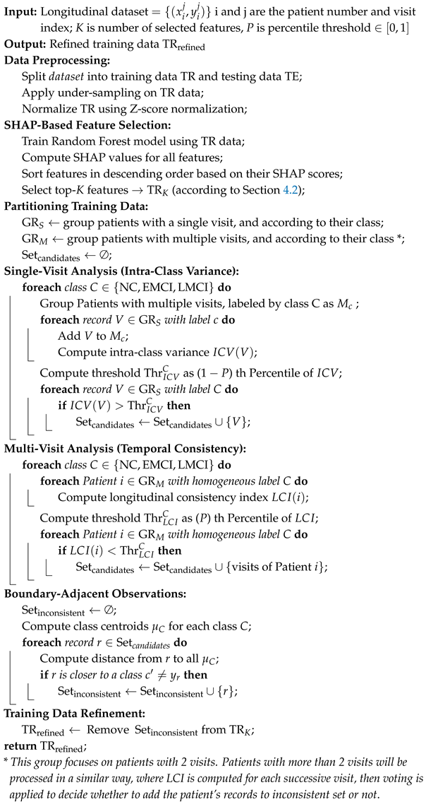
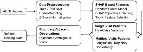
The Alzheimer’s disease dataset contains patients’ measurements across multiple visits (longitudinal data). Certain patient records exhibit class label variability and inaccurate biomarker evaluation [24,26,33]. This is due to dynamic changes in patient cognition, such as psychological state. Another reason is that inaccuracies in biomarker evaluation may arise due to noise or subjective assessment. This negatively affects the efficiency of ML algorithms. In this article, we focus on identifying a subset of patients’ records that cause this inconsistency in the scope of mild cognitive impairment disease at different stages. This study identifies candidates among these records that increase intra-class variance and reduce the coherence of the longitudinal trajectory for patients with a single visit and patients having a similar class label across multiple visits, respectively. Furthermore, these candidates are checked to determine whether they are marginal patterns. The proposed method is depicted in Figure 1, while the detailed steps are shown in Algorithm 1.
Figure 1.
Proposed distributional coherence–based data refinement method.
4.1. Data Preprocessing
This stage comprises a sequence of standard procedures. The data has 3827 records with 378 measures representing patients’ data across five modalities.
| Algorithm 1: Distributional Coherence-Based Data Refinement |
 |
There are 341 numerical and 37 categorical features, respectively. First, the data are split into training and testing sets at an 80:20 ratio. The splitting process ensures that entire patient visits are assigned exclusively to either the training set or the testing set, thereby preventing data leakage. The class distribution for the training data is 45.2%, 38.6%, and 16.2% for patient records labeled as NC, EMCI, and LMCI, respectively. Since the training data is imbalanced, under-sampling of the majority classes is applied to address class imbalance, resulting in a reduced training set of 1479 patient records. The third procedure is feature scaling, which is applied by fitting a z-score normalization to the training data to achieve a mean of zero and a standard deviation of one. This procedure is essential to mitigate feature-scale bias.
4.2. SHAP-Guided Feature Selection
This phase is crucial when the training set has a large number of features relative to the size of the patient records. Therefore, feature selection is applied to identify the most relevant features for the given classes. Motivated by recent studies in feature selection, Shapley Additive exPlanations (SHAP) is employed as a feature selection technique [31,32,35]. SHAP quantifies the feature contribution to an individual prediction relative to the model’s average output. SHAP is a post hoc explanation technique that helps identify meaningful patterns learned by a machine learning model. For this purpose, a Random Forest classifier is first fitted on the training set [35]. Subsequently, SHAP is applied to the trained model to compute contribution values for all features. The features are then ranked in descending order (based on their contribution scores), and the top-K features are selected for use in subsequent stages.
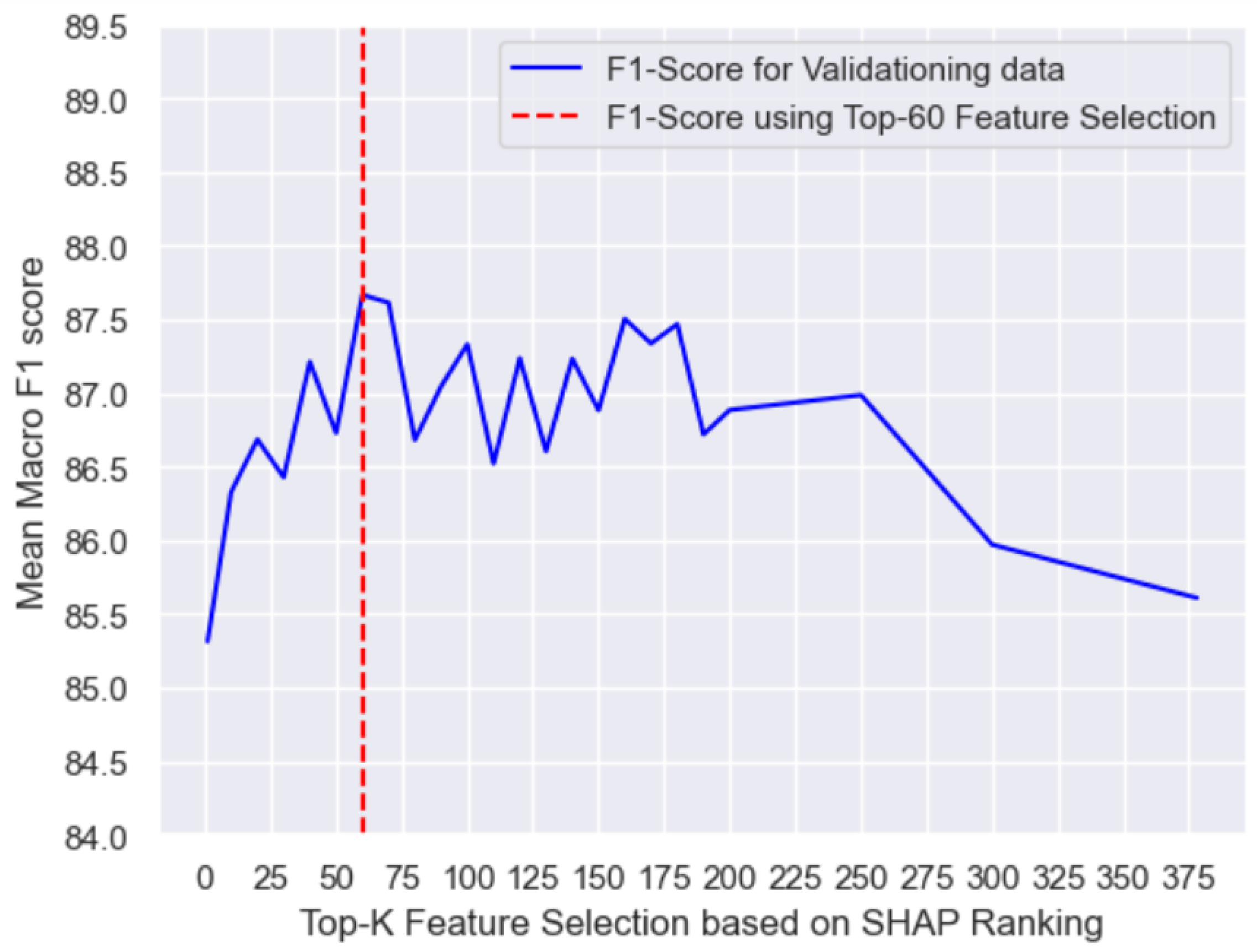
The setting of K is based on the following processes. First, check the cumulative contribution when analyzing all feature importance using SHAP, then identify the Elbow point that strikes a balance between reducing error and avoiding overfitting. Based on these results, feature selection sets with different K values are evaluated during random forest training. During this process, validation scores are monitored, where stratified 5-fold cross-validation is applied to provide a reliable estimate of generalization performance. The K is empirically chosen to reflect the corresponding top-K feature selection that leads to high validation performance, and it should be located near the Elbow point.
4.3. Detecting Patient Visits with Potentially Ambiguous Observations
This phase aims to identify patient visits that are distributionally atypical records, meaning they deviate from the typical records within the same class. This includes single-visit patients that appear as outliers, as well as multi-visit patients whose longitudinal trajectories do not align with the expected progression of others sharing the same class label. Such inconsistent visits in feature space tend to lie closer to neighboring classes than to their assigned class, indicating potentially distributionally atypical records.
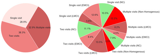
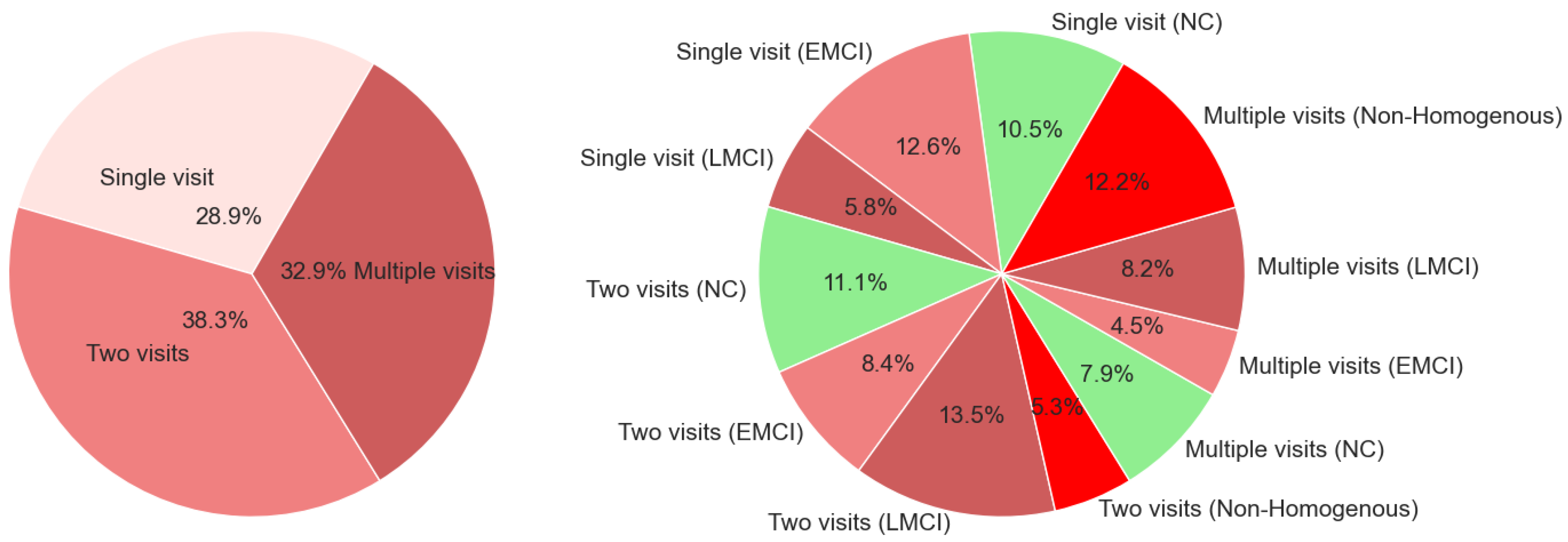
First, the training data are partitioned into three groups: patients with a single visit, two visits, and multiple visits, as illustrated in Figure 2 (left). The corresponding distribution of patients across mild cognitive impairment stages (NC, EMCI, and LMCI classes) is detailed in Figure 2 (right). The proposed algorithm identifies distributionally atypical records among patients with homogeneous (same) class labels across successive visits and with a single visit. Accordingly, based on the training distribution data in Figure 2, the algorithm operates on approximately 82.5% of the given training data. Among patients with different class labels across visits (non-homogeneous), 70.4% of patient records exhibit monotonic class label changes (such as ) and 29.6% of patient records have inconsistent class label transitions (for example, ). The following sections describe how to identify distributionally atypical records.
Figure 2.
Distribution of patients’ visits in the training data.
4.3.1. Patients with a Single Visit
This group lacks longitudinal patient data. Since the patient has a single visit, the proposed method focuses on identifying distributionally distorted records in typical patient visits in each class. This will detect outlier records, hence reducing intra-class variance. Therefore, the intra-class variance (ICV) is introduced here to filter out typical patient visits from distributionally distorted visits. It quantifies the dispersion of samples within each class when each patient’s record is assigned to their corresponding class. N and are the number of patient visits in the group with patient i having a single record in the K feature space, respectively, while is the average measure for biomarker j across N patients who belong to the same group. The following formula computes intra-class variance, where ICV measures the average squared distance between each patient’s visit and the corresponding class center:
Intra-class variance is evaluated separately for each class by incorporating each patient visit into the corresponding multi-visit group having the same class label before estimating its intra-class variance. This procedure enables quantification of the marginal impact of individual visits on intra-class variance within their respective groups. After that, the intra-class variance threshold for class C is determined considering the percentile setting () th where . Each class has a different threshold, where for multi-visit groups labeled by NC, EMCI, and LMCI, respectively. Then, patient records with ICV values higher than are considered candidates for distributionally atypical records.
4.3.2. Patients with Multiple Visits
The underlying hypothesis here is that patients’ test measurements across successive visits should exhibit certain degrees of similarity when the class label remains unchanged over time. This assumption aligns conceptually with the distributional hypothesis in text representation learning, which asserts that words that occur in similar contexts tend to share similar meanings [36]. Guided by this premise, time-aware analyses of patient visits within each group are conducted to identify visits that deviate from their expected consistency and are flagged as candidates having an inconsistent temporal trajectory.
Time-aware consistency is evaluated for patients with multiple visits. For patients with two visits, the availability of records with the same class label (homogeneous labeling) provides limited temporal information for assessing the longitudinal diagnostic trajectory. Therefore, patients having two visits classified with the same class label are expected to exhibit a certain level of similarity. First, let us define the following parameters:
: the feature vector of the patient at the first visit;
: the feature vector of the patient at the second visit;
: time difference in months from the first to the second visit;
: temporal decay parameter (initialized by 0.5).
The next formula computes the Longitudinal Consistency Index (LCI), as follows:
where is the cosine similarity for patient i having two visits and , and its value is in the range of [−1, 1], where 1 corresponds to a perfect match between these visits. The LCI is based on the intrinsic consistency, , while time-based forgiveness is . The first term magnifies the closeness between patient visits. The latter term emphasizes the similarity while penalizing the time difference between the two visits. The objective of the LCI is to impose strong penalties on abrupt changes occurring within short time intervals while gradually relaxing penalties for low similarity across longer durations between visits. First, the consistency index is computed for each patient’s visits, where the (P) th value is chosen as . After that, the patient visits with LCI less than are flagged as inconsistent candidates.
Patients with more than two visits enable convenient time-aware analysis. The is computed similarly to patients with two visits. First, the LCI for each patient with multiple visits is computed considering each successive visit pair and . After that, the (P) th value of LCI scores is chosen as . When the majority of patients’ visits have LCI scores below the threshold , then all patient visits are identified as inconsistent candidates due to low longitudinal trajectory coherence.
4.4. Boundary-Adjacent Observations
The distributionally atypical records of candidates identified in Section 4.3.1 and Section 4.3.2 are filtered based on their discrimination margins to their associated classes. The locations of these patients’ visits in K-dimensional space are compared with their nearest class, where patients having multiple visits are represented by their base (first) visit. Therefore, the decision is based on computing distances from these candidates to these class centroids, including NC, EMCI, and LMCI. The distributionally atypical records are those that are not located in their associated class. These records are then excluded from the training data. This should reduce intra-class variance and increase inter-class separation, thereby enhancing the discriminative capacity of the data, which typically leads to improved ML model performance.
5. Experimental Results
The proposed method is assessed from various aspects. Initially, the K, and derivation thresholds are discussed. Then, the refined training data is statistically analyzed by computing the Fisher score, inter-class variance, intra-class variance, and Cohen’s f. The classifiers’ performance is evaluated on the original and refined training data. In addition, the cross-model predictive stability is assessed to quantify the degree of joint correctness rate across multiple machine learning algorithms. Lastly, both the percentile threshold (P) th and the impact of data splitting are investigated on the proposed method’s performance.
The experiments were deployed on a workstation equipped with an AMD Ryzen 7 processor (8 cores, 2.9 GHz), an NVIDIA GeForce GTX 1660 Ti GPU, and 32 GB of RAM. The results compare the original with the refined training data. The former contains 1479 patient records in 378-dimensional space, while the refined training data has patient records in the range of 1460 to 1375 (when P is set in the range 0.025 to 0.35), with 60 features. The evaluation uses the macro score that assigns equal importance to all classes. The next equation depicts how to compute , given TP, FP, and FN as the number of correct positive, incorrect positive, and incorrect negative predictions, respectively:
5.1. Top-K Feature Selection and Analysis of Intra-Class Variance and Longitudinal Consistency Index
This section presents relevant analysis of the proposed method, specifically defining how the top-K is derived empirically and how and are computed.
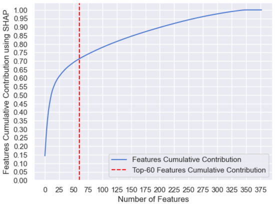
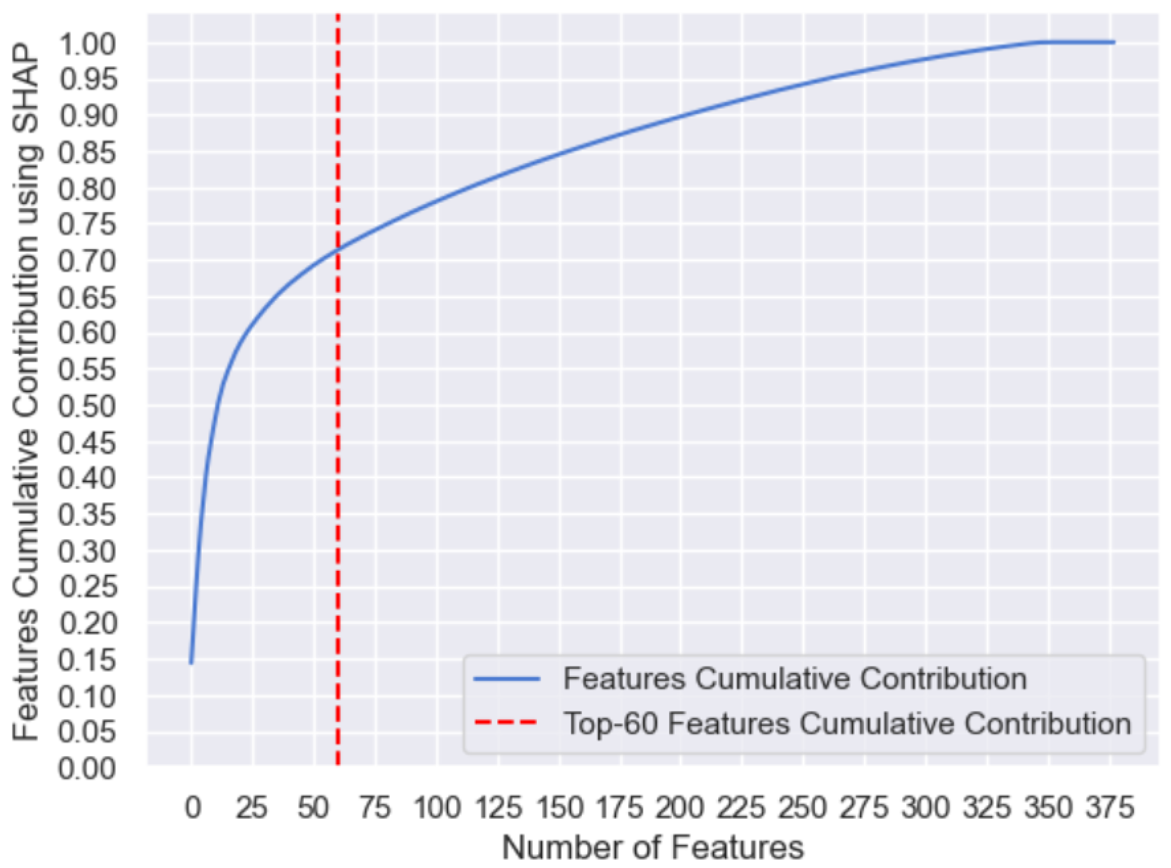
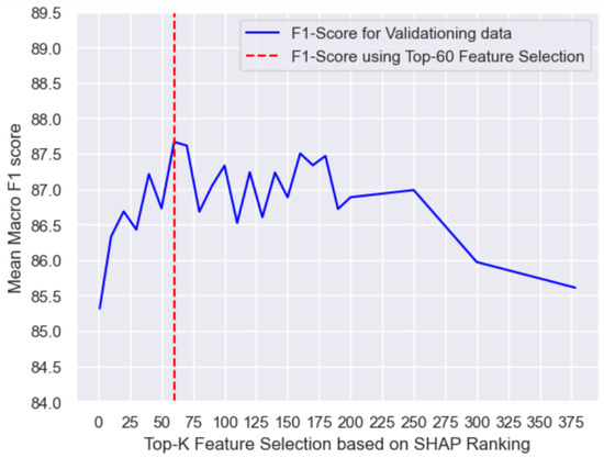
It is crucial to define the top-K features properly. The following presents the results relevant to the steps discussed earlier in Section 4.2. Figure 3 shows the normalized cumulative feature contributions when deploying SHAP for the random forest using all features. According to Figure 3, the first 15 features have more than half the predictive impact when compared to the impact of considering all features (378). When examining the cumulative contribution starting from the first 300 features, it changes very slowly. The suitable value of K lies within the sweet spot, which is between 15 and 200. Then, we train a random forest classifier with various top-K settings and monitor the validation scores, as shown in Figure 4. The value that yields a high validation score and lies within the sweet spot is empirically used to define a suitable top-K setting. Based on Figure 3 and Figure 4, the top-60 features (15.9% of all features) have aggregated contributions of 0.712.
Figure 3.
Feature cumulative contribution based on SHAP analysis.
Figure 4.
score for random Forest using various top-K values.
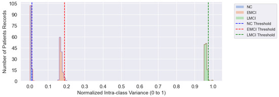
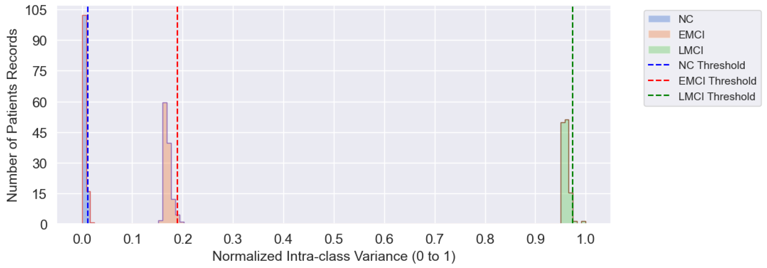
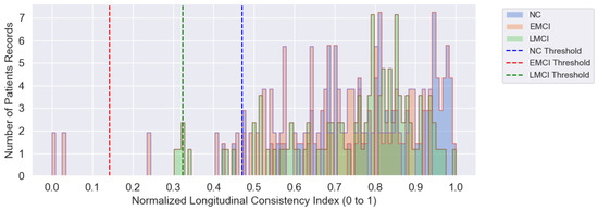
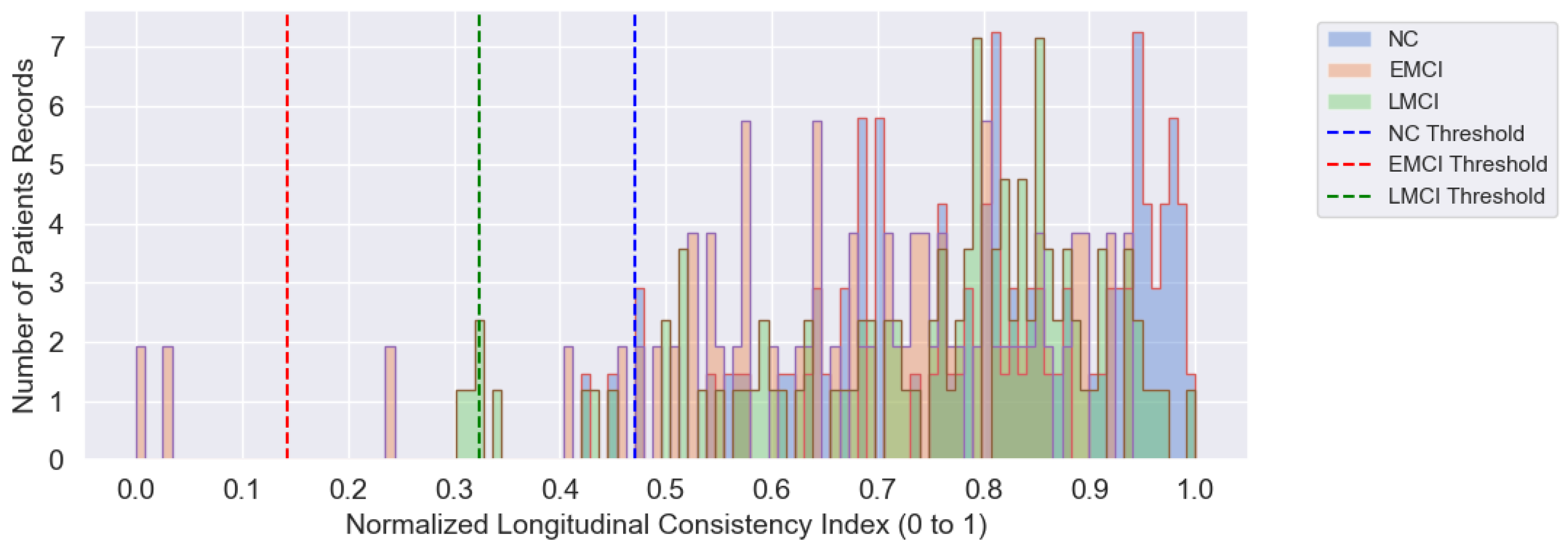
The thresholds for intra-class variance and longitudinal consistency index define the criteria for identifying visits as distributionally atypical. Both thresholds are derived to compute ICV and LCI for patients with single visits and multiple visits, respectively, within each class. Figure 5 shows the histogram of intra-class variance for three classes, NC, EMCI, and LMCI, based on setting the percentile (P) th to 0.025 (where th = 0.975). The dashed line reflects the threshold, (records having percentile). The thresholds for these classes are 0.012, 0.189, and 0.974, respectively. It is observed that the normalized ICV among patients labeled as the NC is significantly lower than that of patients labeled with EMCI and LMCI. This can be explained by the physiological stability of cognitively normal patients, whereas patients with varying degrees of mild cognitive impairment tend to exhibit more diverse symptoms. Figure 6 shows the histogram of LCI when setting the percentile, (P) th, to 0.025 (records having percentile). The thresholds, , are 0.471, 0.142, and 0.323 for the NC, EMCI, and LMCI classes, respectively. Early cognitive impairment has a minimum threshold, which indicates that patients classified as EMCI have less longitudinal trajectory consistency compared to those who have normal cognitive and late cognitive impairment. The candidates discovered so far are processed according to their discrimination margin, as presented in Section 4.4.
Figure 5.
Intra-class variance histogram for NC, EMCI, and LMCI classes.
Figure 6.
Longitudinal consistency index histogram for NC, EMCI, and LMCI classes.
5.2. Data Statistical Evaluation
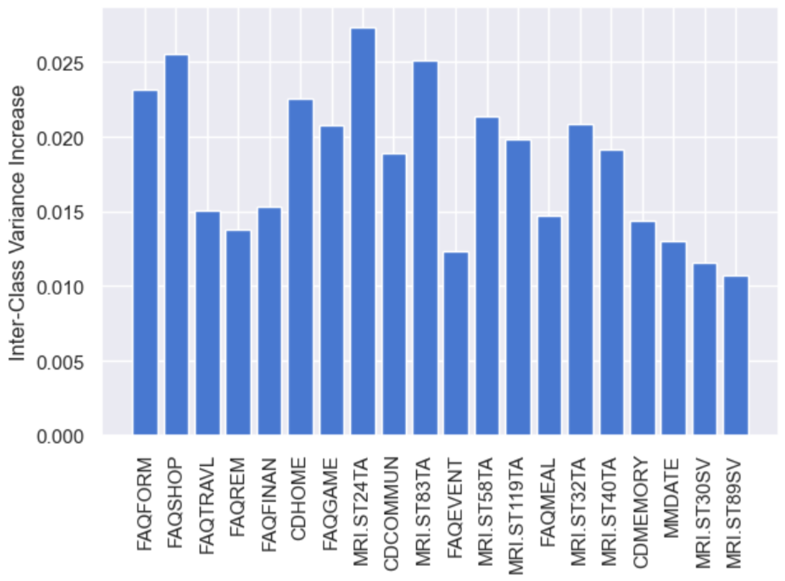
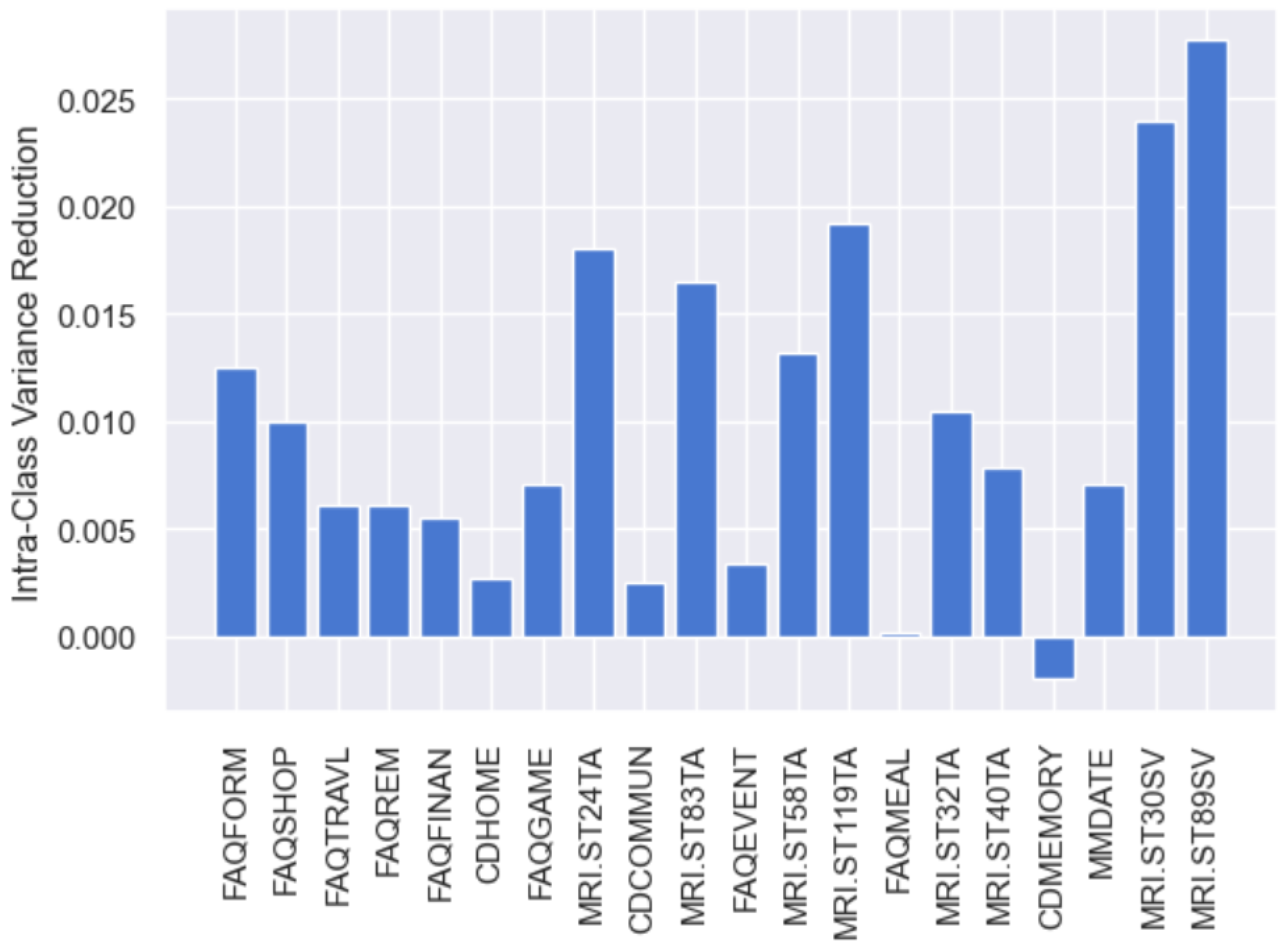
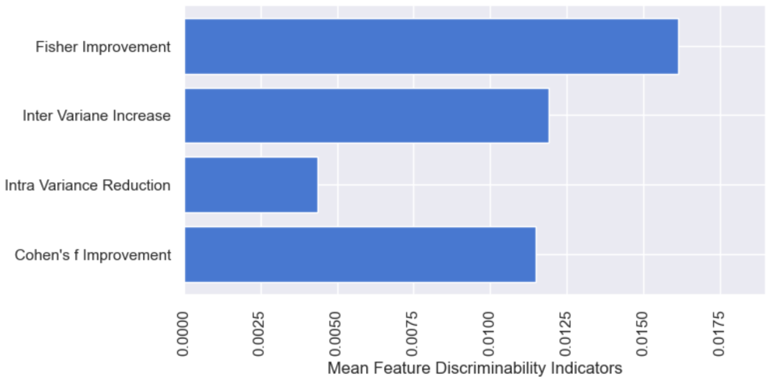
Several statistical analyses have been used to estimate the change in training data after applying the proposed method. The statistical analyses include inter-class variance, intra-class variance, Fisher analysis, and Cohen’s f measures. Inter-class variance reflects class separation, while intra-class variance measures the variation of data points within their respective class centers. Fisher’s analysis is the ratio of inter-class to intra-class variance, and Cohen’s f finds the effect size. These analyses are applied to both the original and refined training data, each having the same 60 features. Percentile (P) th is set to 0.025 when implementing the proposed algorithm. Given the removal of a slight amount of patients’ records, 1.285% of the original training data, the following presents the mean ± standard deviation values for these analyses; they are as follows:
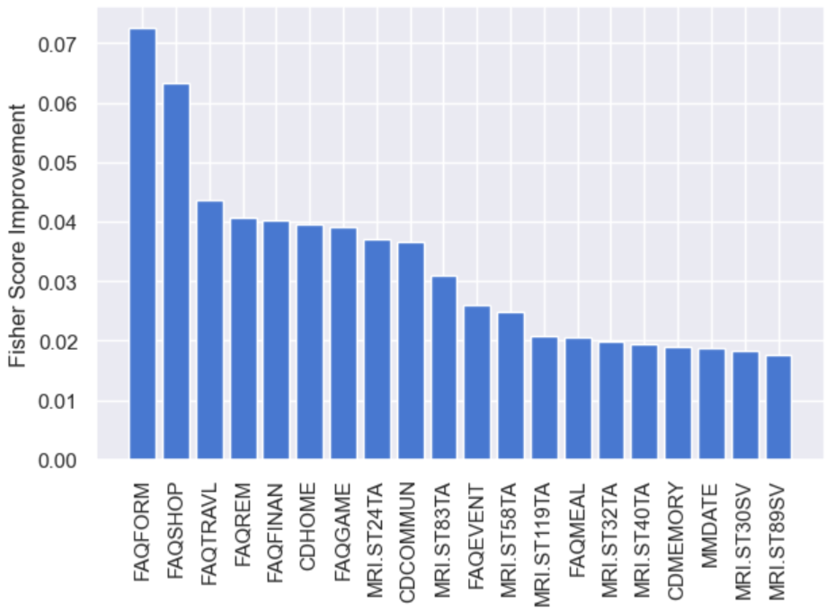
- Fisher score: Gets 0.016 ± 0.015, where FAQFORM gets the maximum improvement while GDMEMORY gets the minimum gain.
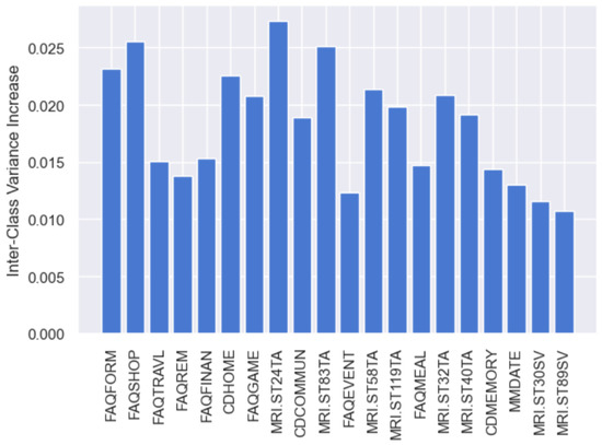
- Inter-class variance: Shows 0.012 ± 0.007, where MRI.ST24TA biomarker has the highest improvements.
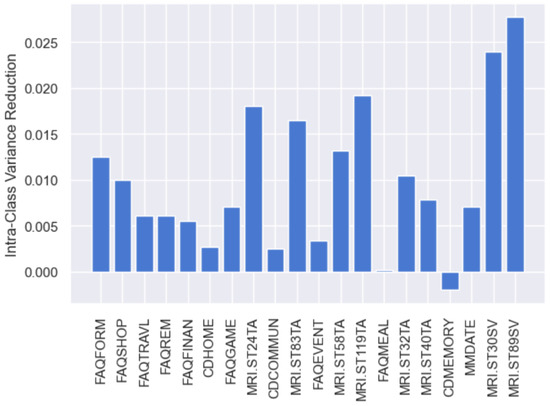
- Intra-class variance: Shows 0.004 ± 0.007, where MRI.ST30SV achieves the maximum reduction among other biomarkers.
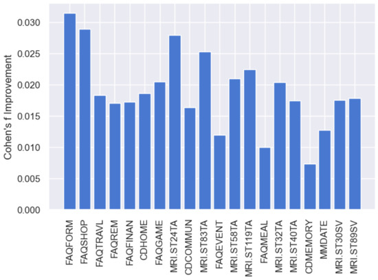
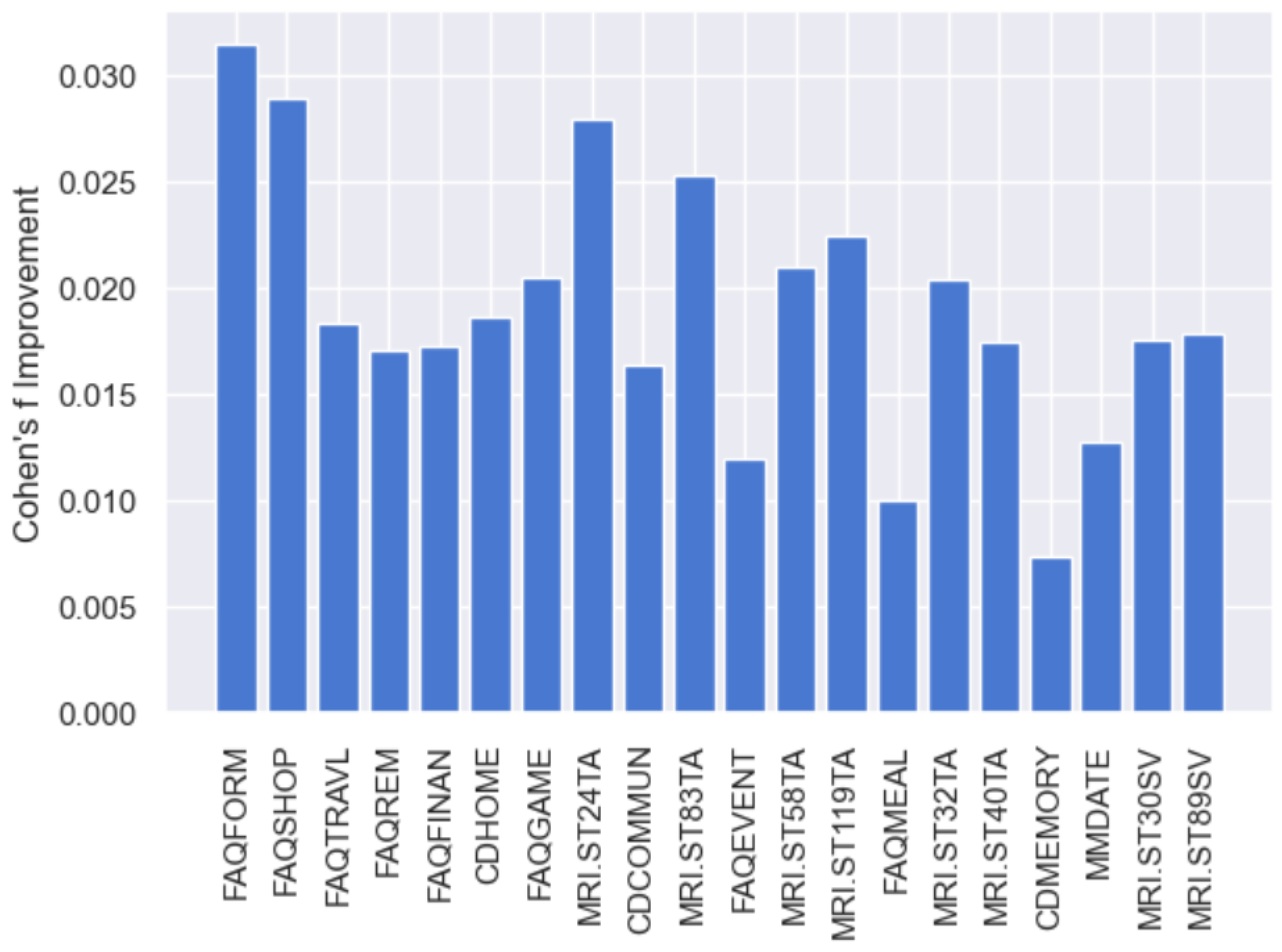
- Cohen’s f: Gets 0.011 ± 0.008, where FAQFORM has the highest improvement.
Figure 7, Figure 8, Figure 9 and Figure 10 show the data analysis for the first 20 features. The average results for these analyses are shown in Figure 11. The removal of a small number of patients’ records leads to a slight increase in Fisher score, inter-class variance, and Cohen’s f, while reducing intra-class variance. Although the effect size is small when assessing the refined training data, it indicates a trend toward increased inter-class distance and decreased intra-class variance. Therefore, the proposed method improves the statistical relevance of class distinctions by suppressing variance components attributable to potentially distributionally atypical records while preserving inter-group differences.
Figure 7.
Fisher score improvement for top-K feature selection.
Figure 8.
Inter-class variance increase for top-K feature selection.
Figure 9.
Intra-class variance reduction for top-K feature selection.
Figure 10.
Cohen’s f improvement for top-K feature selection.
Figure 11.
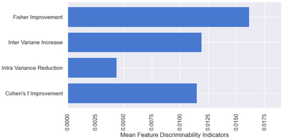
Mean feature discriminability indicators.
5.3. Cross-Model Predictive Stability Analysis
Two machine learning models were used to assess the performance gains achieved by using the refined data: 1460 records with 60 features rather than the original training data; 1479 records with 378 features. These Machine Learning (ML) models are Random Forest (RF) and Neural Networks (NNs). Table 2 presents the configuration settings of these models, which are adjusted to prevent any potential overfitting.
Table 2.
Configuration settings for machine learning models.
Two evaluations were considered for RF and NN models. The first evaluation assesses the extent of improvement in prediction performance achieved when training was conducted on the refined dataset rather than on the original data. The second criterion evaluates the degree of cross-model prediction agreement with respect to the true patient class label when the models are applied to the same test set. This consistency is quantified by the joint correctness rate, defined as the proportion of instances for which both models produce simultaneously correct predictions relative to the ground-truth label. Given that we have two ML models M = 2, N patients’ records, as the prediction of model m for patient record i, and as the true label, the joint correctness rate is defined as:
The average scores for the random forest model are (mean ± standard deviation) 84.035% ± 0.6 and 85.279% ± 0.458, while the average scores are 75.897 ± 1.304 and 80.4 ± 0.707 for the neural network model, when these models are trained on original and refined training data, respectively. These results are based on 10 trials, where the percentile (P) th is set to 0.025 for the distributional coherence-based data refinement method. For the second criterion, the joint correctness rate for the RF and NN models is 69.9% when they use original training data. When these models are trained by the refined data, the joint correctness rate is 74.9% (7.1% improvement). These indicate a potentially better discriminative structure for the refined data than the original data, leading to better model classification performance.
5.4. Effect of Percentile and Splitting the Dataset on the Performance of the Proposed Method
The proposed method relies on the degree of identifying distributionally atypical record candidates using the Percentile (P) th setting, in addition to dataset splitting. The unfiltered training dataset contains 1479 records with 378 features, whereas the refined dataset contains 1460 records with 60 features.
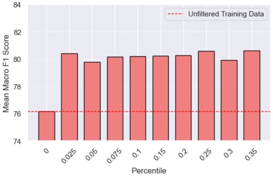
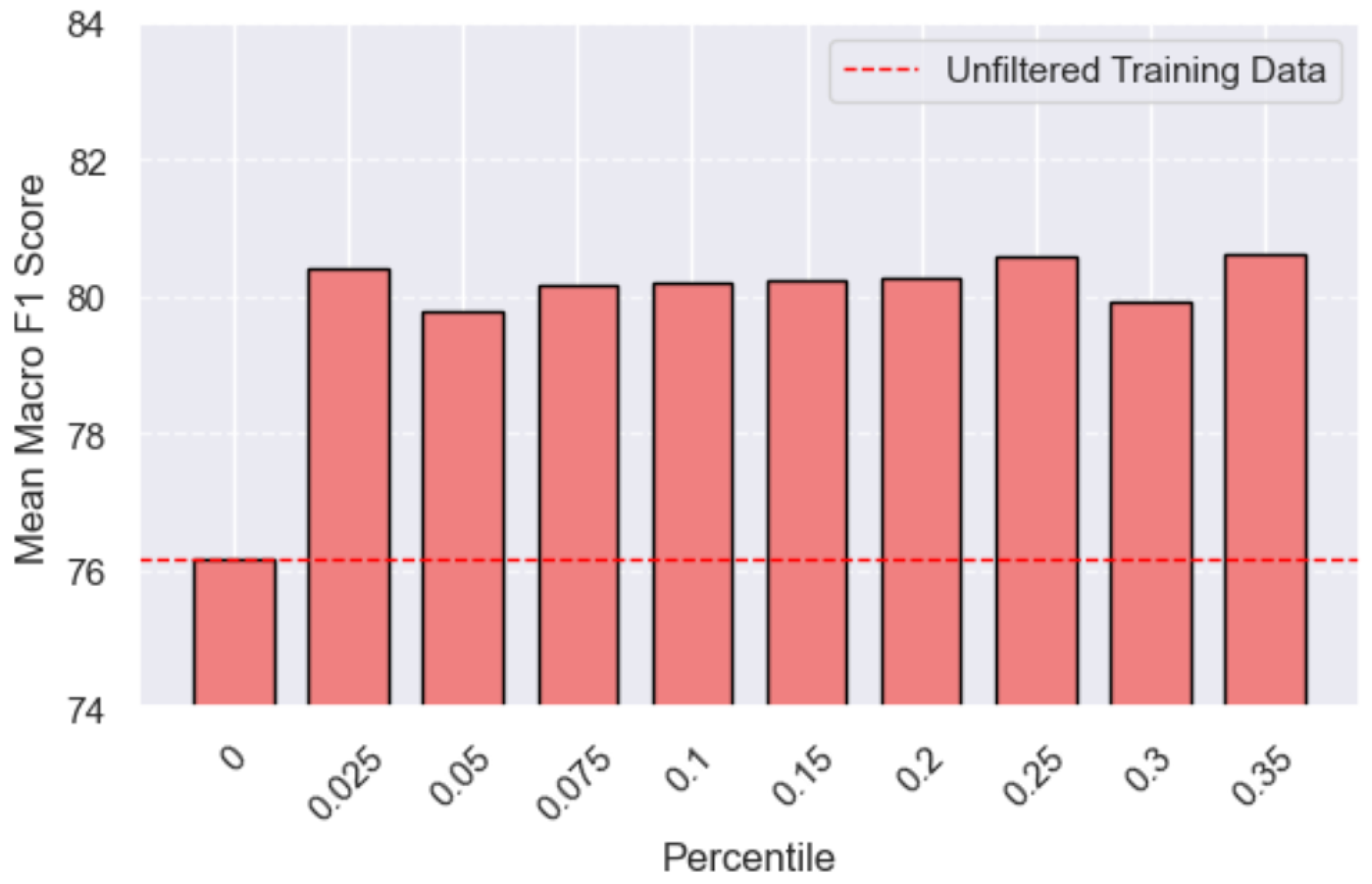
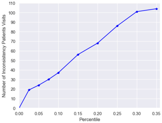
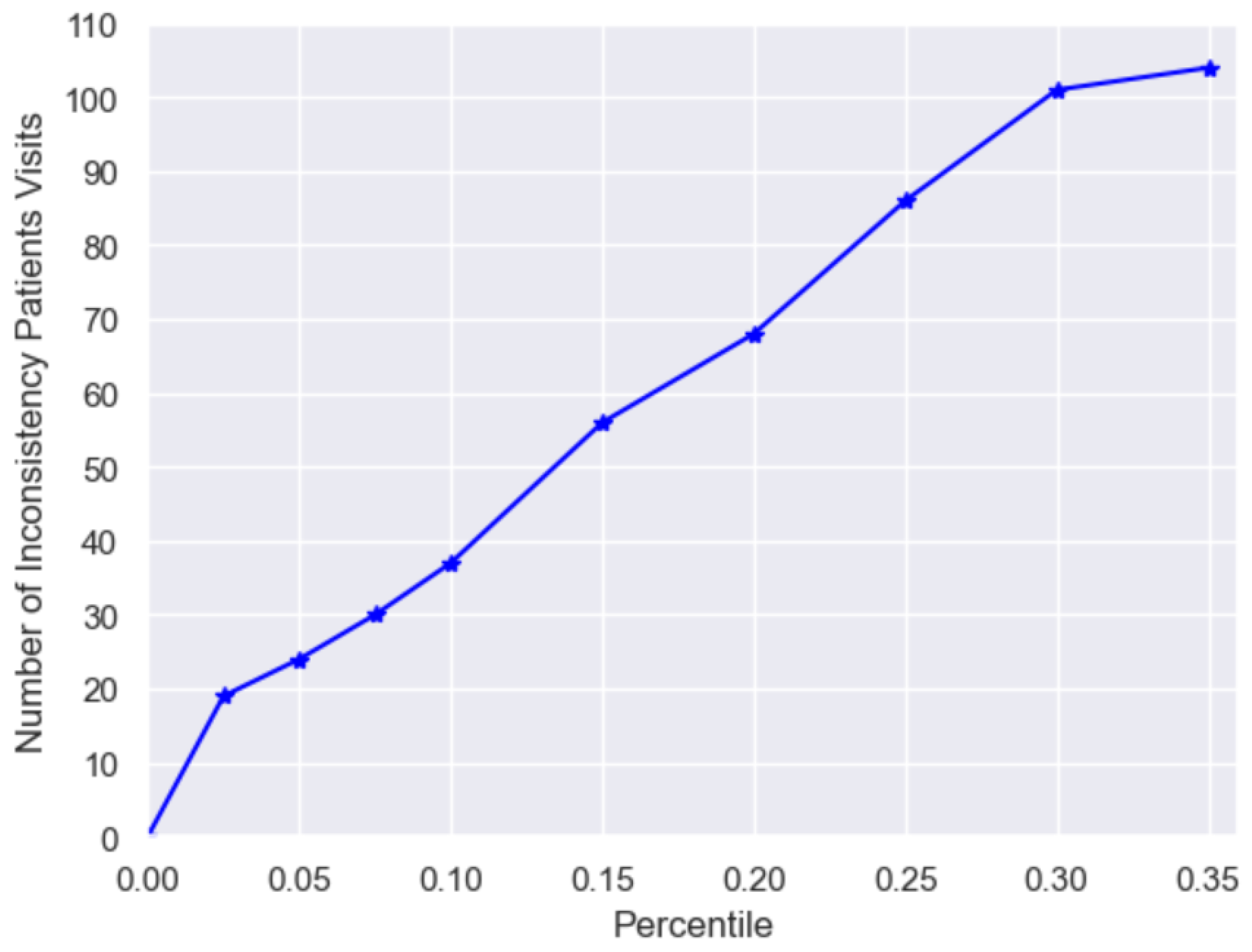
To assess the impact of the percentile parameter P, a neural network model, described in Table 2, was employed. The value of P was empirically predefined in the range of [0.025, 0.35], reflecting a practical interval that balances dataset refinement and sample preservation. Rather than tuning P to maximize predictive performance, this range was selected to evaluate the robustness of the proposed method. The refinement method was applied repeatedly across different P values within this interval. For each configuration, the NN was trained on the refined training dataset, and its prediction performance was evaluated on the test set. The results, illustrated in Figure 12, show that all tested P values yield consistent improvements in score, ranging from 4.5% to 5.5% relative to the baseline model trained on the original dataset (dashed line). Notably, the variation in performance across different P values remains limited, suggesting the following: 1. The method is not sensitive to precise parameter selection, since increasing the percentile threshold beyond a certain range does not further enhance ML prediction, as the proposed method already captures the most influential atypical records while preserving the overall class distribution. 2. The utilization of the boundary-adjacent observation (method’s last stage) includes only candidates’ records detected through the ICV and LCI that lead to a negative discrimination margin. The mean score increased from (mean ± margin of error) 76.17 ± 0.27 to 80.23 ± 0.21, where the confidence interval is 95% following the data refinement method. These results suggest that the proposed method maintains stable predictive performance across the examined percentile range. The Wilcoxon signed-rank test yields a p-value of 0.0625, which does not meet the 0.05 threshold for statistical significance; therefore, the observed improvements should be interpreted as preliminary. Percentile P has a direct impact on the number of detected distributionally atypical records. Figure 13 reflects the relationship between P and the number of excluded patients’ records. It indicates that the relationship is approximately linear. This finding suggests that adopting relatively higher percentile values does not lead to an abrupt increase in the number of records with atypical distribution. This confirms the effect of boundary-adjacent observations, where only distributionally atypical records are detected. Overall, these findings indicate consistent performance improvements to the choice of P, without requiring fine-tuned parameter selection; however, given the lack of statistical significance, these observations should be considered indicative rather than conclusive.
Figure 12.
Mean macro score for neural networks under different P settings.
Figure 13.
Number of inconsistency visits across percentile values.
Random data splitting is essential to ensure that the classifier remains unbiased toward a particular population. Since the proposed method operates on the training data, it is important to measure the effect of applying a random data split on the classifier’s performance when relying on refined training data. Five different data splits are applied. Their refined training sets are used by two classifiers, described in Table 2. The classifier’s results are depicted in Table 3. The p-value for all models is 0.0625, which exceeds the 0.05 threshold and therefore does not indicate a statistically significant difference in performance between classifiers trained on the original and refined datasets across different splits. Nevertheless, the results show a consistent improvement in performance, suggesting a positive but preliminary trend.
Table 3.
Sensitivity of the proposed method to dataset splitting.
6. Discussion
The findings in the results section are interpreted as follows: First, regarding model analysis, selecting K is crucial for high-dimensional datasets to improve ML prediction performance for testing data. According to Figure 3 and Figure 4, increasing K when monitoring the validation scores tends to decrease the model’s performance. Therefore, the sweet spot must be determined, where including features with high predictive contribution would facilitate selecting K empirically. Several studies use SHAP to provide a robust estimation of the features’ contribution. Therefore, SHAP analysis is applied here before examining various top-K settings to reveal features’ contributions and to include the convenient feature selection sets, with various top-K settings during refitting the random forest model.
The threshold settings for both intra-class variance and the longitudinal consistency index are computed from the normalized histograms for patients with single-visit and multiple-visit groups. The histogram of intra-class variance shows that single-visit patients labeled as NC tend to have lower variance, whereas patients with MCI tend to have higher variance. This is clearly visible through the histogram shown in Figure 5. These indicate that NC patients have similar biomarker profiles, in contrast to patients labeled with various degrees of MCI. For patients with multiple visits, the longitudinal trajectory consistency for EMCI is lower than that of corresponding patients classified with NC or LMCI. The patients classified as EMCI tend to have a wide spectrum of symptoms across multiple visits, leading to a low LCI threshold compared to those labeled by other classes.
Regarding the statistical evaluation of the data, the results reveal several advantages and limitations when analyzing the refined training data in comparison with the original training data. Given the small size of distributionally atypical records (1.285% of the original training data), the average increase in Fisher score, inter-class variance, and Cohen’s f, in addition to the average decrease in intra-class variance, are shown in Figure 11. These improvements indicate that the proposed method enhances the intrinsic statistical structure of the training dataset by increasing class separability while simultaneously reducing within-class dispersion. These observations show that distributionally atypical records were effectively suppressed without diminishing meaningful between-group differences. It is observed that a subset of biomarkers benefits from deploying the proposed method. Features such as FAQFORM, MRI.ST24TA and MRI.ST30SV maintained the improvements through these statistical analyses. Regarding the limitations, the analysis reveals that the impact is quite small. The average improvement of inter-class variance is much higher than that of intra-class variance. This indicates that the improvements are not very large but are noticeable between classes more than within the same classes. Overall, the proposed method provides a more coherent representation of class structure. This suggests that the refined training data better capture the underlying disease-related patterns, thereby providing a potentially more stable foundation for downstream ML modeling.
The experimental results demonstrate a consistent improvement in predictive performance for both the RF and NN models when trained on the refined dataset. Specifically, the RF model shows an increase in average score from (mean ± standard deviation) 84.035% ± 0.60 to 85.279% ± 0.458, indicating improved classification performance across the 10 trials. Similarly, the NN model exhibits a more noticeable gain, with the mean score increasing from 75.897 ± 1.304 to 80.400 ± 0.707. This substantial improvement suggests that the refinement process enhances the accuracy of the NN model, which is typically more sensitive to noise and data quality. In addition to individual model performance, the joint correctness rate shows a 7.1% improvement after data refinement (from 69.9% to 74.9%). This indicates an improvement in the global discriminative structure of the training data.
The outcomes derived from investigating the impact of using percentile (P) th and dataset splitting are essential. Setting P with small values yields consistent gains (4.5 to 5.5%). Although these results provide positive insight into the application of the proposed method, the Wilcoxon signed-rank test indicates that the effect of P shows a trend toward significance. This could be explained by the small amounts of the detected distributionally atypical records, that is, in the range of (1.285% to 7.032%). Setting P does not detect a high number of patients’ records, as shown in Figure 13. Therefore, there is almost a linear relationship between P and the number of potentially ambiguous patterns in feature space. On the other hand, data splitting provides different training data populations. According to the results presented in Table 3, the refined training data derived using the proposed method enable machine learning algorithms to achieve more accurate predictions than those obtained using the original training data. Although these results demonstrate a positive impact across different dataset splits, the Wilcoxon signed-rank test indicates that the improvement is not statistically significant (p-value = 0.0625).
Based on these results, the proposed distributional coherence-based training set refinement method may be considered a promising data-centric strategy for improving model performance. Although not intended as a mandatory component of machine learning pipelines, the findings provide a preliminary proof-of-concept that such refinement can serve as an effective complementary step within ML workflows. Nevertheless, the reported outcomes should be interpreted cautiously due to the lack of external dataset validation and expert medical assessment.
7. Study Limitations and Future Work
The following are the study’s limitations, equipped with the corresponding future work:
- Percentile P is set to low values regardless of the choice of machine learning model. Since the machine learning model relies on the quality of refined training data, the selection of P should be linked to the ML model characteristics.
- There is a need to investigate the robustness of the proposed method under alternative preprocessing strategies. The study lacks the required analysis when using different under-sampling strategies and their impact on the method’s performance. This is a critical point to investigate as essential future work. Additionally, the study removes all records with missing data to avoid potential noise generated by data imputation. Still, it is important to investigate the impact of different approaches for missing data imputation on the method’s performance.
- Although SHAP-based feature selection is a robust technique, alternative methods from the filter-based, wrapper-based, and embedded categories require comprehensive investigation.
- The method operates on a subset of patient records. There is a strong need to extend it to include patients with varying class labels across multiple visits. Additionally, the article focuses on mild cognitive impairment at various stages; however, it is essential to consider AD to evaluate the method across the full spectrum of disease stages.
- The detected distributionally atypical records require validation by medical experts to assess the proposed method’s results. Furthermore, the study requires evaluation on independent Alzheimer’s disease datasets to assess the robustness of the proposed method within the AD domain.
- The proposed method has shown promising results for the given dataset. The method needs to be evaluated on other longitudinal datasets to realize its benefits across various domains.
8. Conclusions
The article introduces a data refinement method to detect a subset of distributionally atypical records, thereby supporting the classification of patients with different levels of mild cognitive impairment. The method is based on applying SHAP-based feature selection, checking intra-class variance and longitudinal trajectory, and considering the discrimination margin. The detected distributionally atypical records with single visits are those that increase their class variance while causing a negative margin. For patients with multiple visits, the distributionally atypical records indicate that the dynamic change for these patients’ records does not follow the majority of the longitudinal trajectory, as those patients’ visits belong to the same class.
Based on the statistical analysis results, the refined data show a trend for increasing inter-class distance and decreasing intra-class variance when compared with the original training data. The refined training data supports various machine learning algorithms, such as Random Forest and Neural Networks, to make better predictions of unseen patients’ records. This predictive improvement for these models is based on the proposed method’s ability to exclude 1.285% of the original training data, identified as distributionally atypical records. These models have better decision-boundary stability, which improves the joint correctness rate when classifying unseen patients’ records. Additionally, the method does not detect a large number of patients’ records when using different percentile P settings. Furthermore, varying the P settings or applying random dataset splits shows only a limited impact on the method’s performance. Collectively, these results establish a proof-of-concept for a data-centric refinement approach, highlighting its potential to enhance machine learning model performance beyond conventional preprocessing steps. While not a replacement for standard preprocessing pipelines, the proposed method demonstrates value as a complementary strategy for potentially improving the quality of training data.
Several future research directions arise from the study’s scope and limitations. The current evaluation is conducted on a dataset that does not consider an explicit Alzheimer’s disease class and focuses on patients with the same class label, which may limit its generalization to AD datasets. Additionally, although the refinement process removes a relatively small subset of records, the observed performance improvements, while consistent, did not reach statistical significance. Building on these observations, future work should investigate alternative feature selection strategies beyond SHAP-based techniques to assess their impact in identifying distributionally atypical records. Expanding the method to include patients with different class labels across multiple visits would allow for a more comprehensive evaluation of longitudinal patterns. Moreover, applying the proposed approach to datasets with the full disease spectrum, including explicit AD classes, is essential to get broader validity. Another important direction is to incorporate records with missing values through carefully designed imputation strategies, as these visits may contain valuable information about disease progression. Finally, evaluating the method on longitudinal datasets beyond the current domain would provide further insight into its general applicability.
Funding
This research received no external funding.
Institutional Review Board Statement
Not applicable.
Informed Consent Statement
All authors have read and agreed to the published version of the manuscript.
Data Availability Statement
The data were obtained from the Alzheimer’s Disease Neuroimaging Initiative (ADNI) database, available from https://adni.loni.usc.edu/ (accessed on 24 January 2026). As such, the investigators within the ADNI contributed to the design and implementation of ADNI and/or provided data but did not participate in the analysis or writing of this article.
Acknowledgments
Data used in the preparation of this article were obtained from the Alzheimer’s Disease Neuroimaging Initiative (ADNI) database (https://adni.loni.usc.edu/ (accessed on 20 January 2026)). The authors sincerely thank the reviewers for their constructive comments, which helped improve the paper’s quality.
Conflicts of Interest
The author declares no conflicts of interest.
Abbreviations
The following abbreviations are used in this manuscript:
| AD | Alzheimer’s Disease |
| ML | Machine Learning |
| RF | Random Forests |
| NN | Neural Networks |
| SHAP | SHapley Additive exPlanations |
| NC | Normal Cognitive |
| EMCI | Early Mild Cognitive Impairment |
| LMCI | Late Mild Cognitive Impairment |
| ICV | Intra-class variance |
| LCI | Longitudinal Consistency Index |
References
- Christodoulou, R.; Woodward, A.; Pitsillos, R.; Ibrahim, R.; Georgiou, M. Artificial Intelligence in Alzheimer’s Disease Diagnosis and Prognosis Using PET-MRI: A Narrative Review of High-Impact Literature Post-Tauvid Approval. J. Clin. Med. 2025, 14, 5913. [Google Scholar] [CrossRef] [Scilit]
- Dara, O.A.; Lopez-Guede, J.M.; Raheem, H.I.; Rahebi, J.; Zulueta, E.; Fernandez-Gamiz, U. Alzheimer’s Disease Diagnosis Using Machine Learning: A Survey. Appl. Sci. 2023, 13, 8298. [Google Scholar] [CrossRef] [Scilit]
- Chang, C.-H.; Lin, C.-H.; Lane, H.-Y. Machine Learning and Novel Biomarkers for the Diagnosis of Alzheimer’s Disease. Int. J. Mol. Sci. 2021, 22, 2761. [Google Scholar] [CrossRef] [Scilit]
- Shukla, A.; Tiwari, R.; Tiwari, S. Review on Alzheimer Disease Detection Methods: Automatic Pipelines and Machine Learning Techniques. Sci 2023, 5, 13. [Google Scholar] [CrossRef] [Scilit]
- Khojaste-Sarakhsi, M.; Haghighi, S.S.; Ghomi, S.M.T.F.; Marchiori, E. Deep learning for Alzheimer’s disease diagnosis: A survey. Artif. Intell. Med. 2022, 130, 102332. [Google Scholar] [CrossRef] [Scilit]
- Sarma, M.; Chatterjee, S. Machine Learning-Based Alzheimer’s Disease Stage Diagnosis Utilizing Blood Gene Expression and Clinical Data: A Comparative Investigation. Diagnostics 2025, 15, 211. [Google Scholar] [CrossRef] [Scilit] [PubMed]
- Chatterjee, S.; Byun, Y.-C. Voting Ensemble Approach for Enhancing Alzheimer’s Disease Classification. Sensors 2022, 22, 7661. [Google Scholar] [CrossRef] [Scilit] [PubMed]
- Ebrahimighahnavieh, M.A.; Luo, S.; Chiong, R. Deep learning to detect Alzheimer’s disease from neuroimaging: A systematic literature review. Comput. Methods Programs Biomed. 2020, 187, 105242. [Google Scholar] [CrossRef] [Scilit]
- Reddy C, K.K.; Rangarajan, A.; Rangarajan, D.; Shuaib, M.; Jeribi, F.; Alam, S. A Transfer Learning Approach: Early Prediction of Alzheimer’s Disease on US Healthy Aging Dataset. Mathematics 2024, 12, 2204. [Google Scholar] [CrossRef] [Scilit]
- Dua, M.; Makhija, D.; Manasa, P.Y.L.; Mishra, P. A CNN–RNN–LSTM Based Amalgamation for Alzheimer’s Disease Detection. J. Med. Biol. Eng. 2020, 40, 688–706. [Google Scholar] [CrossRef] [Scilit]
- Odusami, M.; Maskeliūnas, R.; Damaševičius, R. Pixel-Level Fusion Approach with Vision Transformer for Early Detection of Alzheimer’s Disease. Electronics 2023, 12, 1218. [Google Scholar] [CrossRef] [Scilit]
- Shah, S.M.A.H.; Khan, M.Q.; Rizwan, A.; Jan, S.U.; Samee, N.A.; Jamjoom, M.M. Computer-aided diagnosis of Alzheimer’s disease and neurocognitive disorders with multimodal Bi-Vision Transformer (BiViT). Pattern Anal. Appl. 2024, 27, 76. [Google Scholar] [CrossRef] [Scilit]
- Assem Sharaf, H.; Hamed Kholief, M.; Said, H.H.M. Time-Variant Transformers for Predicting Alzheimer’s Disease Progression from Longitudinal Data. In Proceedings of the 35th International Conference on Computer Theory and Applications (ICCTA), Alexandria, Egypt, 25–27 November 2025; pp. 365–370. [Google Scholar] [CrossRef] [Scilit]
- Li, R.; Wang, X.; Berlowitz, D.; Mez, J.; Lin, H.; Yu, H. CARE-AD: A multi-agent large language model framework for Alzheimer’s disease prediction using longitudinal clinical notes. npj Digit. Med. 2025, 8, 541. [Google Scholar] [CrossRef] [Scilit]
- Abadir, P.M.; Battle, A.; Walston, J.D.; Chellappa, R. Enhancing care for older adults and dementia patients with large language models: Proceedings of the National Institute on Aging—Artificial Intelligence & Technology Collaboratory for Aging Research Symposium. J. Gerontol. Ser. A 2024, 79, glae176. [Google Scholar] [CrossRef] [Scilit]
- Said, H.H.M.; Kassem, A.H. Remaining Useful Life Prediction Driven by LLMs Using Few-Shot Learning. In Proceedings of the 35th International Conference on Computer Theory and Applications (ICCTA), Alexandria, Egypt, 25–27 November 2025; pp. 198–203. [Google Scholar] [CrossRef] [Scilit]
- Said, H.H.M. Leveraging LLM-Based Few-Shot Learning for Clinical Decision Support in Alzheimer’s Detection. In Proceedings of the 2025 26th International Arab Conference on Information Technology (ACIT), Alexandria, Egypt, 16–18 December 2025; pp. 366–371. [Google Scholar] [CrossRef] [Scilit]
- Alshamlan, H.; Omar, S.; Aljurayyad, R.; Alabduljabbar, R. Identifying Effective Feature Selection Methods for Alzheimer’s Disease Biomarker Gene Detection Using Machine Learning. Diagnostics 2023, 13, 1771. [Google Scholar] [CrossRef] [Scilit]
- Alshamlan, H.; Alwassel, A.; Banafa, A.; Alsaleem, L. Improving Alzheimer’s Disease Prediction with Different Machine Learning Approaches and Feature Selection Techniques. Diagnostics 2024, 14, 2237. [Google Scholar] [CrossRef] [Scilit]
- Menon, P.A.; Gunasundari, R. SHAP-based Feature Selection and Explainable Machine Learning Classification of Alzheimer’s Disease. J. Comput. Anal. Appl. 2024, 33, 798–817. [Google Scholar]
- Yi, F.; Yang, H.; Chen, D.; Qin, Y.; Han, H.; Cui, J.; Bai, W.; Ma, Y.; Zhang, R.; Yu, H. XGBoost-SHAP-based interpretable diagnostic framework for alzheimer’s disease. BMC Med. Inform. Decis. Mak. 2023, 23, 137. [Google Scholar] [CrossRef] [Scilit]
- Sourkatti, H.; Asuroglu, T.; Itkonen, M.; Alahäivälä, A.-L.I.; Tolppanen, A.-M.; Ihalainen, J.; Forsberg, M.M. A comparative feature selection study: Predicting Alzheimer’s disease using primary healthcare and social services data. Inform. Med. Unlocked 2025, 59, 101703. [Google Scholar] [CrossRef] [Scilit]
- Huang, H.; Wang, P.; Pei, J.; Wang, J.; Alexanian, S.; Niyato, D. Deep Learning Advancements in Anomaly Detection: A Comprehensive Survey. IEEE Internet Things J. 2025, 12, 44318–44342. [Google Scholar] [CrossRef] [Scilit]
- Sorino, P.; Lombardi, A.; Lofù, D.; Colafiglio, T.; Ferrara, A.; Narducci, F.; di Sciascio, E.; di Noia, T. Detecting label noise in longitudinal Alzheimer’s data with explainable artificial intelligence. Brain Inform. 2025, 12, 15. [Google Scholar] [CrossRef] [Scilit]
- Frenay, B.; Verleysen, M. Classification in the Presence of Label Noise: A Survey. IEEE Trans. Neural Netw. Learn. Syst. 2014, 25, 845–869. [Google Scholar] [CrossRef] [Scilit]
- Mulder, E.R.; de Jong, R.A.; Knol, D.L.; van Schijndel, R.A.; Cover, K.S.; Visser, P.J.; Barkhof, F.; Vrenken, H. Hippocampal volume change measurement: Quantitative assessment of the reproducibility of expert manual outlining and the automated methods FreeSurfer and FIRST. NeuroImage 2014, 92, 169–181. [Google Scholar] [CrossRef] [Scilit]
- Bernhardt, M.; Castro, D.C.; Tanno, R.; Schwaighofer, A.; Tezcan, K.C.; Monteiro, M.; Bannur, S.; Lungren, M.P.; Nori, A.; Glocker, B.; et al. Active label cleaning for improved dataset quality under resource constraints. Nat. Commun. 2022, 13, 1161. [Google Scholar] [CrossRef] [Scilit] [PubMed]
- Xu, J.; Yang, Y.; Yang, P. Hybrid Label Noise Correction Algorithm For Medical Auxiliary Diagnosis. In Proceedings of the 2020 IEEE 18th International Conference on Industrial Informatics (INDIN), Warwick, UK, 20–23 July 2020; pp. 567–572. [Google Scholar] [CrossRef] [Scilit]
- Wang, S.; Zhang, H.; Kong, W. Multimodal Classification of Alzheimer’s Disease Using Longitudinal Data Analysis and Hypergraph Regularized Multi-Task Feature Selection. Bioengineering 2025, 12, 388. [Google Scholar] [CrossRef] [Scilit] [PubMed]
- Divya, R.; Shantha Selva Kumari, R. Genetic algorithm with logistic regression feature selection for Alzheimer’s disease classification. Neural Comput. Appl. 2021, 33, 8435–8444. [Google Scholar] [CrossRef] [Scilit]
- Yue, L.; Chen, W.; Liu, S.; Chen, S.; Xiao, S. An explainable machine learning based prediction model for Alzheimer’s disease in China longitudinal aging study. Front. Aging Neurosci. 2023, 15, 1267020. [Google Scholar] [CrossRef] [Scilit]
- Oiza-Zapata, I.; Gallardo-Antolín, A. Alzheimer’s Disease Detection from Speech Using Shapley Additive Explanations for Feature Selection and Enhanced Interpretability. Electronics 2025, 14, 2248. [Google Scholar] [CrossRef] [Scilit]
- Khan, S.U.; Albanyan, A.; Bilal, M.; Ullah, S. A genetic programming Rician noise reduction and explainable deep learning model for Alzheimer’s diseases severity prediction. J. Alzheimer’s Dis. 2024, 102, 129–142. [Google Scholar] [CrossRef] [Scilit] [PubMed]
- Weiner, M.W.; Veitch, D.P.; Aisen, P.S.; Beckett, L.A.; Cairns, N.J.; Green, R.C.; Harvey, D.; Jack, C.R.; Jagust, W.; Liu, E.; et al. The Alzheimer’s Disease Neuroimaging Initiative: A review of papers published since its inception. Alzheimer’s Dement. 2013, 9, e111–e194. [Google Scholar] [CrossRef] [Scilit]
- Gómez-Ramírez, J.; Ávila-Villanueva, M.; Fernández-Blázquez, M.Á. Selecting the most important self-assessed features for predicting conversion to mild cognitive impairment with random forest and permutation-based methods. Sci. Rep. 2020, 10, 20630. [Google Scholar] [CrossRef] [Scilit]
- Mikolov, T.; Chen, K.; Corrado, G.; Dean, J. Efficient Estimation of Word Representations in Vector Space. arXiv 2013. [Google Scholar] [CrossRef] [Scilit]

Disclaimer/Publisher’s Note: The statements, opinions and data contained in all publications are solely those of the individual author(s) and contributor(s) and not of MDPI and/or the editor(s). MDPI and/or the editor(s) disclaim responsibility for any injury to people or property resulting from any ideas, methods, instructions or products referred to in the content. |
© 2026 by the author. Licensee MDPI, Basel, Switzerland. This article is an open access article distributed under the terms and conditions of the Creative Commons Attribution (CC BY) license.