AI-Driven Biopsychosocial Screening for Breast Cancer: Enhancing Risk Prediction via Differential Evolutionary Linear Discriminant Analysis for Feature Extraction

Abstract

In Mexico, the high prevalence and mortality rates associated with breast cancer (BC) constitute a critical public health challenge that demands context-specific preventive measures. This study proposes an integrative framework for predicting BC risk based on a biopsychosocial model. We hypothesize that emotional suppression and repression act as key neuroendocrine disruptors and predisposing factors within the Mexican female population. To test this, we systematically compared the predictive performance of various machine learning classification models using the clinical, psychological, and combined profiles of 110 women. These models were evaluated with and without the application of a robust evolutionary algorithm: Differential Evolutionary Linear Discriminant Analysis for Feature Extraction $(DE-LD{A}_{FE}$). The results demonstrated that integrating clinical and psychological data into a combined latent space significantly improved the performance of the classification algorithms. The Artificial Neural Network achieved the highest metrics (0.9975 Precision; 0.9976 F1-score). However, due to the inherent “black-box” nature of these models (limited clinical interpretability), the Decision Tree emerged as the optimal practical alternative, providing highly competitive (0.8874 Precision; 0.8853 F1-score) and interpretable results. These findings provide empirical evidence that psychological factors, rather than being mere incidental comorbidities, could be associated with the etiology of breast cancer and be used as risk factors in predicting the disease. Ultimately, this AI-driven biopsychosocial screening model offers a scalable, low-cost, and context-adapted risk assessment tool for early BC diagnosis in Mexican women.

1. Introduction

Breast cancer (BC) is the most prevalent neoplasm in women worldwide. Nationally, it has been the most frequent and deadliest cancer affecting Mexican women since 2006 (

Table A1. Epidemiological profile of Breast Cancer in Mexico (2022). Data presents the distribution of incidence (new cases) and mortality stratified by age group, along with the federal entities reporting the highest rates.

Variable	Incidence (New Cases)	Mortality (Deaths)
Reported Total	31,043	8195
By Age Group
20–44 years	7839 (23.0%)	1162 (13.2%)
40–59 years	14,846 (43.5%)	3555 (40.5%)
>60 years	11,430 (33.5%)	4061 (46.3%)
States with Highest Rates	1. Colima	1. Mexico City
(Top 3)	2. Durango	2. Nuevo León
	3. Jalisco	3. Chihuahua

in Appendix A) [1,2,3,4]. With projections estimating over 50,000 new annual cases by 2050, BC represents an urgent and expanding public health challenge. There is broad consensus that early detection is essential to reduce morbidity and mortality. While mammography remains the gold standard for screening programs worldwide, it presents limitations. Widespread mammographic screening is often restricted by age guidelines and carries concerns regarding radiation exposure, particularly for younger populations [5,6,7]. This is especially relevant in Mexico, where advanced-stage BC is frequently diagnosed in women aged 20–41 [8,9]. Since 2013, our group has developed non-radiographic resources to identify young Mexican women at elevated risk, aiming to optimize early detection while minimizing unnecessary radiation exposure.

Although the Official Mexican Standard [10] acknowledges that biological, iatrogenic, reproductive, and lifestyle factors interplay to determine BC relative risk, current national screening programs rely almost exclusively on biological and reproductive history. This approach has not substantially reduced incidence or mortality rates, likely because these factors explain, at best, 50% of BC prevalence. We have recently suggested that the accuracy of risk identification would increase by incorporating psycho-affective factors into screening designs [11,12]. Evidence suggests that specific personality traits—such as low emotional containment, low defensiveness, and high stress—are consistently observed in Mexican women with BC prior to diagnosis [11]. Physiologically, emotional suppression and repression are known to alter diurnal cortisol secretion, a dysregulation associated with early mortality in metastatic BC patients [13,14]. Furthermore, principal component analyses have demonstrated that healthy women and those with benign or malignant breast lesions cluster differentially when emotional suppression, repression, and stress symptoms are included in the phenotyping [12]. Notably, when clinical and psychological variables are analyzed together, emotional suppression variables significantly define differential group clustering. These observations support the hypothesis that screening for psychological factors is crucial for prevention, early diagnosis, and understanding BC pathogenesis [15,16,17,18,19].

To improve risk identification in young Mexican women, García-Camacho et al. [20] previously designed a decision tree-based model assessing the Stress Symptom Inventory (ISE), the Courtauld Emotional Control Suppression Scale (CECS), and the Weinberger Adjustment Inventory (WAI). Their results showed that while these tools achieved low accuracy individually (34–40%), their combination improved prediction to 42.7%. This suggests that while the emotional dimension has discriminatory value, the modeling approach required refinement to achieve clinical utility.

On the other hand, recent advances in biopsychosocial risk prediction and explainable AI highlight the importance of integrating multi-domain data for oncology applications. Hussain et al. [21] reviewed machine learning approaches for breast cancer risk prediction, emphasizing the added value of psychosocial variables in enhancing model accuracy. Similarly, radiomics-based studies have demonstrated that multimodal feature fusion, such as parenchymal enhancement and breast symmetry in MRI, improves discrimination power in early detection [22]. In parallel, evolutionary feature extraction methods have been increasingly applied in oncology, as shown by Wang et al. [23], who underscored the role of metaheuristic optimization in refining tumor subtype classification. Explainable AI (XAI) frameworks, such as those discussed by Carriero et al. [24], further stress the necessity of transparency in clinical models, particularly when integrating heterogeneous data sources.

Beyond breast cancer, comparable strategies have been successfully deployed in other medical domains. The NEDL-GCP model [25] introduced a nested ensemble deep learning framework for gynecological cancer risk prediction, demonstrating how ensemble architectures can robustly manage complex clinical datasets. Doumari et al. [26] proposed a novel high-accuracy model for the early diagnosis of Parkinson’s disease, illustrating the potential of feature-fusion and classifier optimization in neurodegenerative contexts.

Building on this foundation, we present a new risk assessment model that employs Differential Evolutionary Linear Discriminant Analysis for Feature Extraction ($DE-LD{A}_{FE}$). This approach integrates biological, reproductive, and psychological variables to manage the complexity of the dataset. Unlike previous models, $DE-LD{A}_{FE}$ simplifies the observation of risk classes and reveals the synergistic behavior of the data. Furthermore, this work is distinguished by its focus on the Mexican population and its key innovation: the use of psychological data alongside clinical data—an approach that, unlike our group [11,12,27], no other previous study in the country has integrated into breast cancer risk assessment, a gap that this work seeks to fill. Although the analyzed cohort consists of 110 individuals, it accurately represents the psychological and clinical information of Mexican women, a group in which identifying risk factors for breast cancer is a priority.

The $DE-LD{A}_{FE}$ method was used to improve classification using machine learning algorithms, prioritizing those that offer explainability in their results. This approach lays the groundwork for future applications, such as the development of a web module that estimates breast cancer risk in an accessible, non-invasive, highly accurate, and timely manner.

2. Methodology

2.1. Participants and Study Design

This study utilized clinical and psychological data from 150 women attending routine gynecological consultations at the General Hospital of Mexico “Dr. Eduardo Liceaga.” All participants provided written informed consent, ensuring confidentiality and anonymity in accordance with the Declaration of Helsinki (printed in the British Medical Journal, 18 July 1964).

The sample was selected to represent a broad age range (see

Table A2. Clinical and social characteristics of the participants.

	BC (n = 50) %	BBP (n = 50) %	H (n = 50) %
Age group
16–19	0	6	0
20–29	6	14	34
30–39	14	28	14
40–49	30	26	28
50–59	26	24	18
60–69	10	0	6
>70	14	2	0
Marital status
Never married	16	36	58
Married	44	34	32
Free union	18	16	4
Divorced or Separated	6	8	6
Widowed	16	6	0
Years of education
0	6	0	0
1–6	52	26	10
7–12	30	46	16
13–18	12	14	50
>19	0	14	24
Family history of cancer
Yes	40	56	46
No	60	44	54
Menarche
Early 8–10 years	1	2	2
Normal 11–12 years	23	27	28
Late ≥ 13 years	26	21	20
Menopause
Yes	24	7	10
No	26	43	40
Childbirths
Yes	37	23	24
No	13	27	26
Hormone replacement therapy
Yes	25	10	4
No	25	40	46
IMC
Normal 18.5–24.9	12	15	22
Overweight 25.0–29.9	26	22	13
Obesity ≥ 30	12	12	15

in Appendix A), reflecting the epidemiological reality of BC in Mexican women; it is frequently diagnosed approximately a decade earlier than global averages [5]. Participants were recruited prior to histopathological diagnosis and were subsequently stratified into three groups based on their clinical pathology reports. The Healthy Group (H, n = 50) clustered women with no palpable or radiological breast pathology. The Benign Breast Pathology Group (BBP, n = 50) was formed by women diagnosed with fibrocystic changes, fibroadenomas, or mastitis. The Breast Cancer Group (BC, n = 50) included women diagnosed with infiltrating ductal carcinoma (naïve to treatment).

2.2. Data Collection Instruments

Physical, hereditary, and lifestyle data were collected using a 57-item General Data Questionnaire. Psychological profiles—specifically emotional repression, suppression, and stress symptomatology—were assessed using three validated instruments:

2.2.1. Inventory of Stress Symptoms (ISE)

Designed by Benevides-Pereira et al. [28], the ISE evaluates the frequency of stress manifestations in daily life across three dimensions: psychological, physical, and social symptoms. It consists of 30 items rated on a 5-point Likert scale (0 = never to 4 = always). Global symptomatology scores are categorized as low (0–22), medium (22–33), or high (>33).

2.2.2. Courtauld Emotional Control Scale (CECS)

Developed by Watson and Greer [29] and validated for Spanish speakers by Durá et al. [30]. The CECS assesses the extent to which individuals suppress reactions to negative emotions. It comprises 21 items across three subscales: Anger, Anxiety, and Depression. Higher scores indicate greater emotional suppression. The instrument demonstrates high internal consistency (α = 0.95). For this study, a median split (score = 32) was used to categorize participants into “Emotional Suppression” (score ≥ 32) or “Emotional Expression” (score < 32) groups.

2.2.3. The Weinberger Adjustment Inventory (WAI)

The WAI [31,32,33] evaluates adjustment styles through three primary scales: Subjective Distress, Restraint, and Defensiveness. The interactions between these scales allow the identification of six typologies of adjustment, including the Repressive (Type C) coping style. The Spanish version validated for the Mexican population [34] was used (Cronbach’s α ranges from 0.69 to 0.89 across subscales).

2.3. Feature Encoding and Binarization

Given the binary nature of the clinical data, and in order to compare them with the results of the psychological instruments, the latter were transformed into dichotomous variables to assess the presence or absence of certain psychological traits in the groups of women. The psychological data, originally expressed as continuous scores or subscales, were categorized into low, medium, and high levels according to their values. Subsequently, these categories were recoded into binary variables (1 for the presence of the characteristic; 0 for its absence), using cut-off points previously defined and described in Romo-González et al. [27]. In most cases, the original cut-off points for each instrument were retained; however, in the case of the CECS, these were established based on 95% confidence intervals. The specific binarization criteria are detailed in

Table A3. Classification criteria for clinical and psychological study variables.

Clinical Variable	Criterion
Age	40–69 years = 1	Under 40 or over 70 = 0
Family history of cancer (FamHis)	Family members with history of cancer = 1	Family members with no history of cancer = 0
Overweight (OW)	BMI between 25 and 29.9 = 1	Higher or lower than that = 0
Obesity (Obe)	BMI between 30 and 39.9 = 1	Higher or lower than that = 0
Smoking (Taba)	Addiction present = 1	No addiction = 0
Alcoholism (Alco)	Addiction present = 1	No addiction = 0
Drug use (Toxi)	Addiction present = 1	No addiction = 0
Early menarche (EarlyMen)	Younger than 12 years = 1	13 years or older = 0
Late menopause (LateMenop)	50 years or older = 1	49 years or younger = 0
Pregnancies (Preg)	No = 0	Yes = 1
Vaginal delivery (Da)	Presence = 1	Absence = 0
Abortion (Abo)	Presence = 1	Absence = 0
Cesarean section (Cesa)	Presence = 1	Absence = 0
Age at first delivery (AFD)	Younger than 30 =0	31 years or older = 1
Use of exogenous hormones (EH)	Yes = 1	No = 0
Breastfeeding (Lac)	Did not breastfeed = 1	Did breastfeed = 0
Hormone replacement therapy (HRT)	Uses HRT = 1	Does not use HRT = 0
CECS Evaluation Criteria
Variable		Criterion
Low Anger (AL)	0–15 = 1	Greater than 15 = 0
Middle Anger (AM)	16–18 = 1	Below 16 or above 18 = 0
High Anger (AH)	Greater than or equal to 19 = 1	Less than 19 = 0
Low Depression (DL)	0–15 = 1	Greater than 15 = 0
Middle Depression (DM)	16–18 = 1	Below 16 or above 18 = 0
High Depression (DH)	Greater than or equal to 19 = 1	Less than 19 = 0
Low Anxiety (ANL)	0–15 = 1	Greater than 15 = 0
Middle Anxiety (ANM)	16–18 = 1	Below 16 or above 18 = 0
High Anxiety (ANH)	Greater than or equal to 19 = 1	Less than 19 = 0
Low CECS (SL)	0–50 = 0	Greater than 50 = 0
Middle CECS (SM)	51–55 = 1	Below 51 or above 55 = 0
High CECS (SH)	Greater than or equal to 56= 0	Less than 56 = 0
WAI Evaluation Criteria
Variable		Criterion
DSL (Low)	Less than 47 = 1	Above 47 = 0
DSH (High)	Less than 47 = 0	Above 47 = 1
RL (Low)	Less than or equal to 94 = 1	Above 94 = 0
RM (Middle)	95–107 = 1	Below 95 or above 107 = 0
RH (High)	Greater than or equal to 108 = 1	Less than 108 = 0
RDL (Low)	Less than 58 = 1	Greater than 58 = 0
RDH (High)	Less than 58 = 0	Greater than 58 = 1
ISE Evaluation Criteria
Variable		Criterion
Low Physical (SFL)	0–5 = 1	Greater than 5 = 0
Middle Physical (SFM)	6–8 = 1	Below 6 or above 8 = 0
High Physical (SFH)	Greater than or equal to 9 =1	Less than 9 = 0
Low Psychological (SPL)	0–11 = 1	Greater than 11 = 0
Middle Psychological (SPM)	12–19 = 1	Below 12 or above 19 = 0
High Psychological (SPH)	Greater than or equal to 20 = 1	Less than 20 = 0
Low Social (SSL)	0–5 = 1	Greater than 5 = 0
Middle Social (SSM)	6–8 = 1	Below 6 or above 8 = 0
High Social (SSH)	Greater than or equal to 9 = 1	Less than 9 = 0
Low Global (SGL)	0–22 = 1	Less than 22 = 0
Middle Global (SGM)	23–32 = 1	Below 23 or above 32 = 0
High Global (SGH)	Greater than or equal to 33 = 1	Less than 33 = 0

of Appendix A. Appendix C examines the potential loss or gain of information resulting from the binarization of psychological data.

2.4. Machine Learning Identification Model

To manage dataset complexity and achieve optimal separation among the three groups (H, BBP, and BC), a supervised learning approach, Differential Evolutionary Linear Discriminant Analysis for Feature Extraction ($DE-LD{A}_{FE}$), was employed. This method performs dimensionality reduction while enhancing class separability by combining linear transformations of the original variables with evolutionary optimization to obtain a projection matrix that maximizes class separation in a two-dimensional space. The following sections describe the main components of this method.

2.4.1. Projection-Based Dimensionality Reduction

Let $X\in {\mathbb{R}}^{m\times n}$ be a dataset with $m$ samples and $n$ features. The goal is to obtain a reduced representation $Y\in {\mathbb{R}}^{m\times d}$, with $d=2$, defined as:

$$Y=XW$$

(1)

where $W\in {\mathbb{R}}^{n\times d}$ is the projection matrix whose columns are orthonormal vectors. This transformation produces new features that are linear combinations of the original variables, while orthonormality ensures that the columns form a valid basis for the projected space.

2.4.2. Differential Evolution Optimization

Differential Evolution (DE) is a population-based optimization method that iteratively refines a set of candidate solutions using mutation, crossover, and selection operators.

At iteration (generation) $g$, the population consists of $N$ candidate solutions (individuals) randomly initialized within the domain of a fitness function $f$. Each individual is represented by a vector ${\mathbf{x}}_{\mathbf{i}}\in {\mathbb{R}}^d$, where $d$ denotes the dimensionality of the problem. In the DE-LDA_{FE} framework, each individual corresponds to a vector ${\mathbf{w}}_{\mathbf{i}}\in {\mathbb{R}}^{n\times d}$ that encodes a candidate projection matrix $W_{\mathrm{i}}\in {\mathbb{R}}^{n\times d}$, with $d=2$, as presented in Equation (2). The particularity of these matrixes is that they are orthonormal by columns, to define the projection directions.

$$W_i=\left(\begin{array}{cc}{w}_{11}& w_{12}\\ w_{21}& w_{22}\\ ⋮& ⋮\\ w_{n1}& w_{n2}\end{array}\right)\iff {\mathbf{w}}_{\mathrm{i}}=\left(w_{11} \hspace{1em}{w}_{21} \hspace{1em}\dots \hspace{1em} w_{n1} \hspace{1em}{w}_{12} \hspace{1em}{w}_{22} \hspace{1em}\dots \hspace{1em}{w}_{n2}\right)$$

(2)

The DE/best/1/bin strategy is used. For each target vector ${\mathbf{w}}_{\mathrm{i}}$ in the population, a mutant vector is generated as:

$${\mathbf{v}}_i={\mathbf{w}}_{best}+F({\mathbf{w}}_{r1}-{\mathbf{w}}_{r2})$$

(3)

where ${\mathbf{w}}_{best}$ is the current best solution, ${\mathbf{w}}_{r1},{\mathbf{w}}_{r2}$ are random individuals, and $F$ is the mutation factor.

A trial vector is then created via binomial crossover:

$$u_{i,j}=\left\{\begin{array}{cc}{v}_{i,j}& \mathrm{if}ran{d}_j\le CR\mathrm{or}j=j_{rand}\\ w_{i,j}& \mathrm{otherwise}\end{array}\right.$$

(4)

where $CR$ is the crossover rate, and $j_{rand}$ corresponds to a randomly selected position. The selection step retains the solution with the highest fitness between the trial vector ${\mathbf{u}}_{\mathrm{i}}$ and the target vector ${\mathbf{w}}_{\mathrm{i}}$.

These steps are repeated until a stopping criterion is met, such as reaching a maximum number of generations or population convergence. Thus, through this iterative evolutionary process, the population of candidate solutions is progressively refined by combining and selecting the best individuals at each generation. As a result, the algorithm converges toward projection matrices that increasingly improve class separability, enabling the discovery of a near-optimal solution in the lower-dimensional space.

2.4.3. Fitness Function

For the $DE-LD{A}_{FE}$ method, the quality of each projection is evaluated using Fisher’s discriminant criterion, which seeks to maximize the separation between class means while minimizing the dispersion within each class. This is achieved by maximizing the ratio between the between-class scatter and the within-class scatter in the projected space, as presented in Equation (5).

$$J(W)={\displaystyle \frac{\mid W^T{S}_{B}W\mid }{\mid W^T{S}_{W}W\mid }}$$

(5)

where $S_B$ and $S_W$ represent the between-class and within-class scatter matrices, respectively, as presented in Equations (6) and (7), where $G$ denotes the number of classes, ${\mu }_g$ the mean of class $g$, and $\mu$ the global mean.

$$S_B={\sum }_{g=1}^G{m}_g({\mu }_g-\mu )({\mu }_g-\mu {)}^T$$

(6)

$$S_w={\sum }_{g=1}^G{\sum }_{x\in C_g}\left(x-{\mu }_g\right){\left(x-{\mu }_g\right)}^T$$

(7)

This criterion promotes projections in which samples from the same class are tightly clustered and those from different classes are well separated in the reduced space.

2.5. Evaluation of Classifiers with/Without the $DE-LD{A}_{FE}$ Algorithm

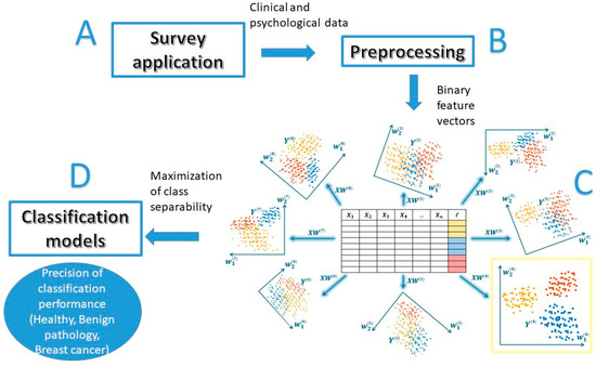
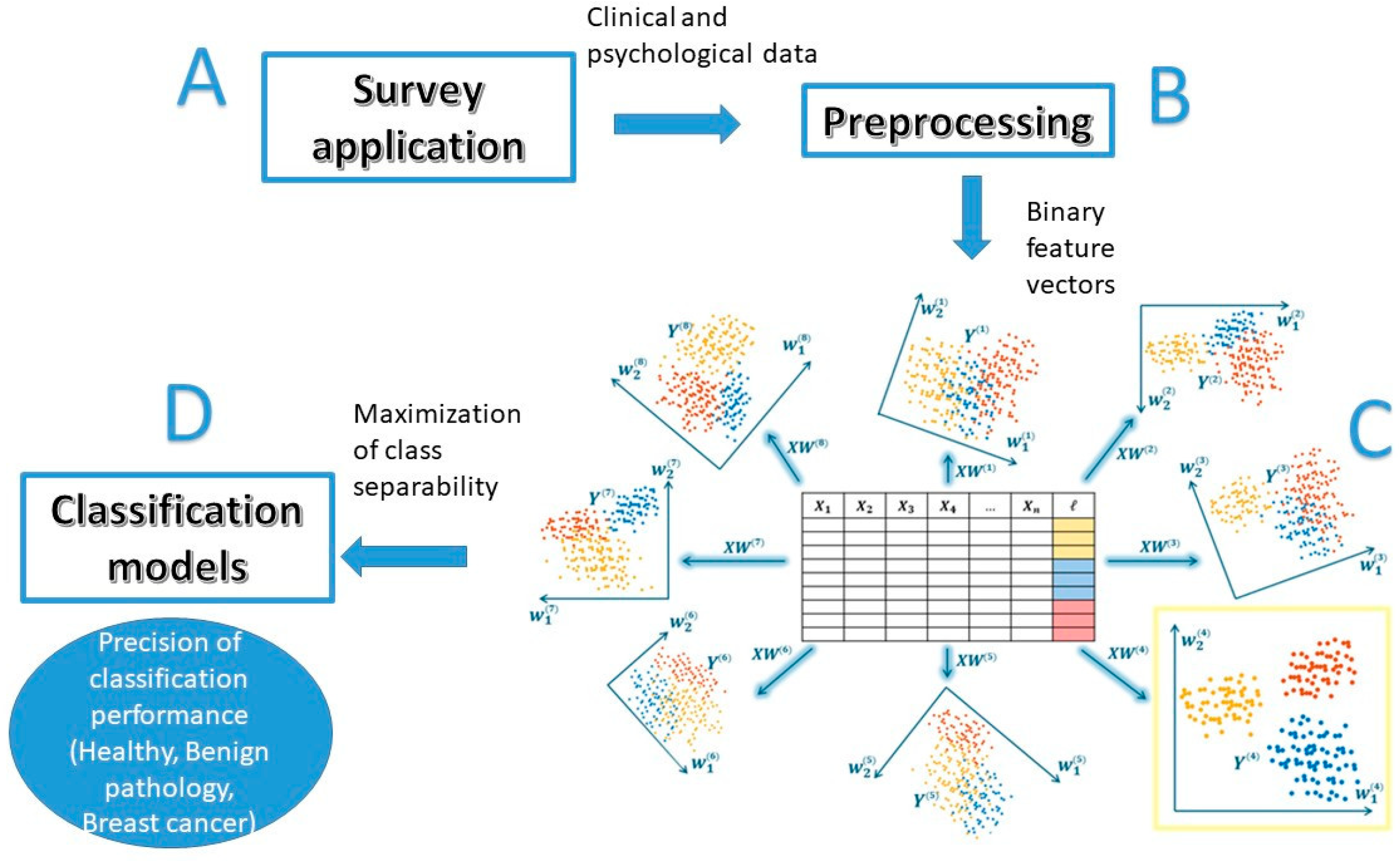
In this research, to analyze the prediction of breast cancer risk by integrating clinical and psychological variables, a comparison of six classification models is performed: K-nearest neighbors (K-nn; k = 3, 5, 7, 9, and 11); Linear Discriminant Analysis (Linear); Gaussian classifier (Gaussian); Decision Tree (DT); Support Vector Machine (SVM); and Artificial Neural Network (ANN). This comparison is made by considering the raw data of the clinical variables, the psychological variables, and finally, both. In addition, the feature extraction method, Feature Extraction ($DE-LD{A}_{FE}$), is used to graphically analyze classification performance and improve the classifier’s accuracy., as presented in Figure 1.

To determine the most suitable Artificial Neural Network (ANN) configuration, a systematic experimental evaluation was conducted using feedforward fully connected neural networks for multiclass classification. The tested architectures consisted of 1 to 5 hidden layers, each with the same number of neurons. The number of neurons per layer was varied across the set {10, 20, 30, 40, 50, 100, 200, 300, 400, 500}, generating a broad range of shallow and deep network configurations. In all cases, each network received the dataset as input and produced class predictions at the output layer. This structured exploration enabled comparison of architectures with different depths and capacities to identify the configuration that achieved the best classification performance according to the selected evaluation metrics.

For the $DE-LD{A}_{FE}$ method, a grid search strategy was employed by systematically exploring combinations of the Differential Evolution (DE) parameters, including population size $N\in \{100,300,500,1000,2000\}$, number of generations $NG\in \{300,500,700,900\}$, crossover rate $CR\in \{0.3,0.5,0.7\}$, and scale factor $F\in \{0.3,0.5,0.7\}$. The best classification values were obtained with the configurations shown in

Table 1. Parameter settings used for the $DE-LD{A}_{FE}$ method across the experiments for each dataset.

Parameter	Clinical	Psychological	Both
Population size (N)	2000	2000	300
Generations (NG)	300	300	700
Crossover rate (CR)	0.5	0.5	0.5
Mutation rate (F)	0.3	0.3	0.7

for each data type.

3. Results

This section presents the comparative performance of the selected classification models in predicting BC risk using clinical, psychological, and integrated datasets. Following the exclusion of records with missing data, a final cohort of 110 patients (out of the original 150) was included in the analysis.

Model performance was assessed using both the raw data and data obtained after using the $DE-LD{A}_{FE}$ feature extraction method. To rigorously evaluate the classifiers, standard performance metrics were utilized, including True Positive (TP) Rate, False Positive (FP) Rate, Accuracy, Recall, F1-score, and the Area Under the Receiver Operating Characteristic Curve (AUC-ROC).

For the experiments, the classification performance was evaluated on the training set. This choice was made because the primary goal of the proposed method is to compare the discriminative quality of different feature representations rather than to estimate generalization performance. Although this approach may yield optimistic accuracy values, it ensures a fair and controlled comparison across methods, since all models are evaluated under identical conditions. Additionally, the dataset’s limited size supports the use of this evaluation strategy.

For the raw variables, the results presented consider only one execution, since the dataset employed does not vary; however, for the projections of the variables with the $DE-LD{A}_{FE}$ method, since it is a stochastic, population-based metaheuristic algorithm, the projections are not unique, so the results presented are the mean of 10 runs, and, to perform a fair comparison, the best solution obtained on these 10 runs is employed for comparison with the results of the raw data.

3.1. Classification Based on Clinical Variables

3.1.1. Analysis of Raw Clinical Data

In this initial experimental phase, the classification models were trained using the clinical variables in their original, unprocessed state. This baseline analysis serves to evaluate the inherent discriminatory power of standard biological and reproductive risk factors prior to the application of any feature extraction or dimensionality reduction techniques. The comparative performance metrics for each classifier in this scenario are detailed in

Table 2. Performance metrics of classification models using raw clinical data.

Classification Models	TP RATE	FP RATE	Precision	Recall	F1-Score	AUC-ROC
K-nn (3)	0.6548	0.3673	0.7466	0.6518	0.6690	0.8676
K-nn (5)	0.6326	0.3742	0.6947	0.5972	0.6056	0.8300
K-nn (7)	0.6626	0.4309	0.6547	0.5811	0.5857	0.7790
K-nn (9)	0.6116	0.3990	0.6167	0.5598	0.5575	0.7313
K-nn (11)	0.6164	0.4099	0.5720	0.5167	0.5070	0.7263
Linear	0.6944	0.3978	0.6471	0.5951	0.6076	0.7978
Gaussian	0.7894	0.3757	0.8628	0.7937	0.8064	0.9528
DT	0.7285	0.3272	0.7939	0.6969	0.7165	0.8966
SVM	0.6827	0.4007	0.6892	0.6144	0.6255	0.7856
ANN (30)	0.8519	0.2520	0.9144	0.8964	0.9034	0.9892

Classification models: K-Nearest Neighbors (K-nn), Linear Discriminant Classifier (Linear), Gaussian Classifier (Gaussian), Decision Tree (DT), Support Vector Machine (SVM), Artificial Neural Network (ANN). The optimal ANN architecture consists of two hidden layers with 30 neurons each.

.

As shown in Table 1, the performance of classifiers trained on raw clinical data varied significantly depending on the algorithm’s architecture. The ANN with 30 neurons demonstrated superior predictive capability, achieving the highest scores across all metrics, with an F1-score of 0.9034 and an AUC-ROC of 0.9892. The Gaussian classifier also performed robustly, securing the second-best performance (F1-score: 0.8064).

Conversely, the K-nn algorithm exhibited an inverse relationship between the number of neighbors (K) and model performance; as K increased from 3 to 11, the F1-score progressively declined from 0.6690 to 0.5070. Linear and SVM models yielded moderate results (F1-scores ≈ 0.60–0.62), suggesting that the boundaries between risk groups in the raw clinical space are non-linear and complex, requiring more sophisticated modeling approaches like ANNs to be effectively decoded.

3.1.2. Classification Using Clinical Data Projections via $DE-LD{A}_{FE}$ Method

As established in previous sections, the $DE-LD{A}_{FE}$ method was implemented to improve class separation by projecting the original variables into an optimized, lower-dimensional latent space. This projection aimed to enhance the discriminative performance of the classification models. The average performance metrics obtained using these clinical projections, calculated over 10 independent runs, are presented in

Table 3. Average performance metrics of classification models using clinical variable projections via $DE-LD{A}_{FE}$ method.

Classification Models	TP RATE	FP RATE	Precision	Recall	F1-Score	AUC-ROC
K-nn (3)	0.6835	0.3416	0.7810	0.7096	0.7273	0.8937
K-nn (5)	0.6549	0.3478	0.7141	0.6553	0.6673	0.8586
K-nn (7)	0.6823	0.3984	0.6926	0.6262	0.6370	0.8228
K-nn (9)	0.6705	0.3812	0.6795	0.6010	0.6137	0.8039
K-nn (11)	0.6601	0.3885	0.6684	0.5879	0.5997	0.7961
Linear	0.6914	0.3993	0.6504	0.5986	0.6101	0.7940
Gaussian	0.6795	0.3993	0.6745	0.6031	0.6159	0.7808
DT	0.7360	0.3227	0.8043	0.7733	0.7831	0.9089
SVM	0.6902	0.3953	0.6645	0.5822	0.5952	0.7993
ANN (400)	0.8238	0.3226	0.9111	0.8911	0.8990	0.9875

Classification models: K-Nearest Neighbors (K-nn), Linear Discriminant Classifier (Linear), Gaussian Classifier (Gaussian), Decision Tree (DT), Support Vector Machine (SVM), Artificial Neural Network (ANN). The optimal ANN architecture comprises two hidden layers with 400 neurons per layer.

.

As indicated in Table 3, the models demonstrating the highest predictive capability when utilizing the projected clinical variables were the ANN architecture with 400 neurons (Precision: 0.9111; F1-score: 0.8990) and the DT model (Precision: 0.8043; F1-score: 0.7831). The remaining models exhibited moderate, comparable performances. Consistent with the raw data findings, the K-nn model displayed a decline in both Precision and F1-score as the number of neighbors (K) increased, confirming that K = 3 remains the optimal configuration for this spatial mapping.

While Table 3 reflects the average robustness across 10 iterations, it is also highly relevant to identify the peak potential of each classifier.

Table 4. Best individual run performance for each classification model using clinical variable projections.

Classification Models	Experiment	TP RATE	FP RATE	Precision	Recall	F1-Score	AUC-ROC
K-nn (3)	10	0.6895	0.3396	0.8008	0.7173	0.7380	0.8966
K-nn (5)	2	0.6462	0.3432	0.7587	0.6922	0.7080	0.8520
K-nn (7)	10	0.6787	0.3933	0.7401	0.6504	0.6644	0.8235
K-nn (9)	3	0.6765	0.3910	0.7012	0.6343	0.6492	0.8059
K-nn (11)	8	0.6752	0.3829	0.6939	0.6292	0.6455	0.8148
Linear	1	0.6935	0.3995	0.6703	0.6041	0.6204	0.7967
Gaussian	8	0.6784	0.4004	0.6865	0.6092	0.6250	0.7797
DT	8	0.7268	0.3246	0.8234	0.7842	0.7935	0.9125
SVM	7	0.6890	0.3972	0.6779	0.5907	0.6049	0.7981
ANN (400)	3	0.8379	0.2829	0.9149	0.8947	0.9024	0.9894

Classification models: K-Nearest Neighbors (K-nn), Linear Discriminant Classifier (Linear), Gaussian Classifier (Gaussian), Decision Tree (DT), Support Vector Machine (SVM), Artificial Neural Network (ANN).

details the single best-performing run for each model based on the clinical projections.

The results in Table 4 mirror the trends observed in the average metrics, reaffirming the superiority of the ANN model. Notably, the peak performance was achieved during Experiment 3 using an expanded architecture of 500 neurons, which yielded an exceptional Precision of 0.9149 and an F1-score of 0.9024. The DT model similarly achieved its peak during Experiment 8, solidifying its position as the second most effective classifier for these specific clinical projections.

3.1.3. Performance Comparison: Raw vs. Projected Clinical Data

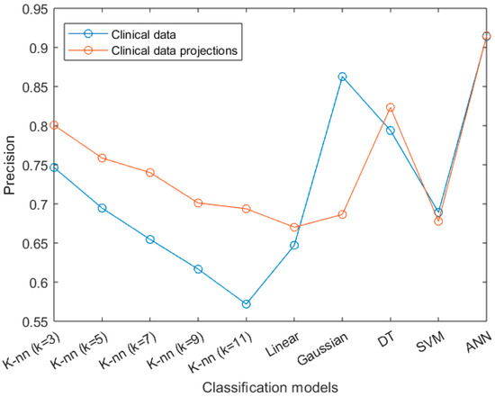
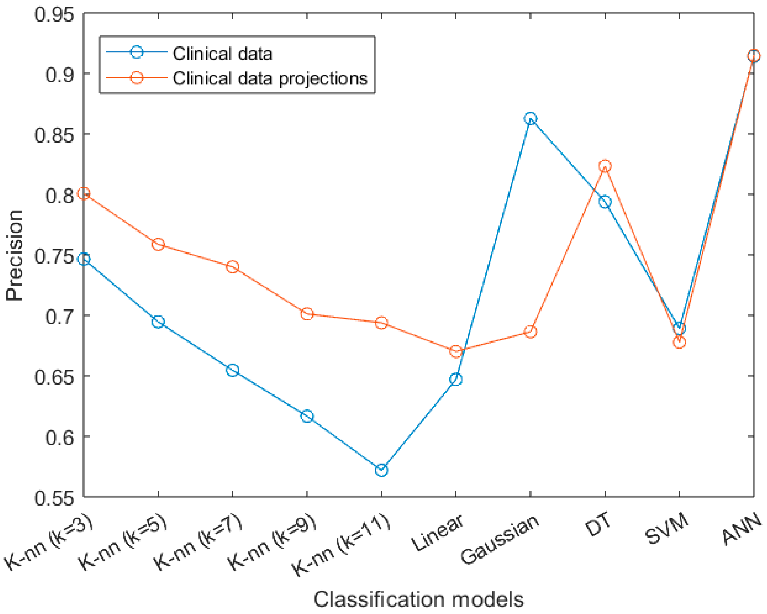
Figure 2 illustrates the comparative performance of the classification models when trained on raw clinical variables versus the optimized latent projections generated by the $DE-LD{A}_{FE}$ method. As observed, for K-nn, DT, SVM, and Linear, the application of the $DE-LD{A}_{FE}$ method successfully enhanced class separability, thereby contributing to an overall improvement in classification metrics.

However, two notable exceptions emerged: Gaussian and ANN classifiers achieved their peak performance using the raw, not projected clinical data. This outcome suggests that these specific non-linear algorithms possess an inherent capacity to map the complex, multi-dimensional relationships of biological risk factors in their original state, without requiring prior dimensionality reduction or feature extraction.

3.2. Classification Based on Psychological Variables

3.2.1. Analysis of Raw Psychological Variables

In this phase of the analysis, the classification models were trained using the raw psychological variables exclusively (without any preprocessing or projection). This experiment establishes a baseline to evaluate the inherent predictive power of psychological factors, such as emotional repression, suppression, and stress, when analyzed in isolation. The comparative performance metrics for each classifier in this raw psychological space are presented in

Table 5. Performance metrics of classification models using raw psychological data.

Classification Model	TP RATE	FP RATE	Precision	Recall	F1-Score	AUC-ROC
K-nn (3)	0.6091	0.4252	0.5689	0.5187	0.5257	0.7865
K-nn (5)	0.5996	0.4416	0.5322	0.4772	0.4575	0.7487
K-nn (7)	0.6601	0.5053	0.4942	0.4668	0.4502	0.7129
K-nn (9)	0.6049	0.4793	0.4735	0.4455	0.4330	0.6717
K-nn (11)	0.6243	0.5184	0.4781	0.4526	0.4385	0.6456
Linear	0.7005	0.4011	0.5999	0.5656	0.5717	0.8036
Gaussian	0.6870	0.3936	0.4780	0.6255	0.5419	0.7983
DT	0.7128	0.3735	0.7402	0.7294	0.7298	0.8796
SVM	0.7223	0.3912	0.6974	0.6158	0.6263	0.8362
ANN (20)	0.8933	0.1779	1.0000	1.0000	1.0000	1.0000

Classification models: K-Nearest Neighbors (K-nn), Linear Discriminant Classifier (Linear), Gaussian Classifier (Gaussian), Decision Tree (DT), Support Vector Machine (SVM), Artificial Neural Network (ANN). The optimal ANN architecture comprises one hidden layer with 20 neurons per layer.

.

As shown in Table 5, the classification models exhibited varying degrees of success when processing the psychological variables. Most notably, the ANN, configured with an optimized hidden layer of 20 neurons, achieved extraordinary, perfect predictive metrics across the board (Precision: 1.0000; F1-score: 1.0000; AUC-ROC: 1.0000). This indicates an absolute separation of the risk classes by the network within this specific training configuration. The DT model emerged as the second most effective classifier for raw psychological data, recording a Precision of 0.7402 and an F1-score of 0.7298. The remaining probabilistic and linear models demonstrated moderate performance. Consistent with the trends observed in the clinical data analysis, the K-nn algorithm displayed an inverse relationship between the number of neighbors (K) and model efficacy; as K increased, both Precision and the F1-score systematically declined, confirming that K = 3 remains the optimal parameter within this configuration.

3.2.2. Classification Using Psychological Data Projections via $DE-LD{A}_{FE}$ Method

Following the same procedure applied to the clinical data, the psychological variables were projected into an optimized latent space using the $DE-LD{A}_{FE}$ method. This transformation aims to maximize class separability and enhance the predictive performance of the classification algorithms. The average performance metrics obtained from these psychological projections, calculated over 10 independent runs, are presented in

Table 6. Average performance metrics of classification models using psychological variable projections via $DE-LD{A}_{FE}$ method.

Classification Model	TP RATE	FP RATE	Precision	Recall	F1-Score	AUC-ROC
K-nn (3)	0.6914	0.3390	0.7708	0.7238	0.7367	0.9129
K-nn (5)	0.6698	0.3393	0.6981	0.6581	0.6667	0.8714
K-nn (7)	0.7004	0.3844	0.6670	0.6401	0.6450	0.8492
K-nn (9)	0.6879	0.3876	0.6535	0.6194	0.6248	0.8350
K-nn (11)	0.6892	0.4129	0.6422	0.6073	0.6125	0.8251
Linear	0.6935	0.4041	0.5941	0.5734	0.5774	0.7934
Gaussian	0.6945	0.4031	0.6147	0.5880	0.5938	0.7954
DT	0.7499	0.3008	0.8224	0.8169	0.8149	0.9339
SVM	0.7000	0.4010	0.6581	0.5918	0.5983	0.8031
ANN (500)	0.8930	0.1876	1.0000	1.0000	1.0000	1.0000

Classification models: K-Nearest Neighbors (K-nn), Linear Discriminant Classifier (Linear), Gaussian Classifier (Gaussian), Decision Tree (DT), Support Vector Machine (SVM), Artificial Neural Network (ANN). The optimal ANN architecture comprises two hidden layers with 500 neurons per layer.

.

As detailed in Table 6, the ANN, dynamically configured with an expanded hidden layer of 500 neurons for this projected space, maintained its perfect predictive capability across the key metrics (Precision: 1.0000; F1-score: 1.0000). The DT model demonstrated notable improvement compared to its raw data baseline, securing the second-highest average performance (Precision: 0.8224; F1-score: 0.8149). The remaining classifiers exhibited similar, moderate performances. Regarding the K-nn model, the inverse relationship between the number of neighbors (K) and model accuracy persisted, confirming K = 3 as the optimal configuration for this projected space.

While Table 6 illustrates the average stability of the classifiers, it is equally important to evaluate their peak predictive potential.

Table 7. Best individual run performance for each classification model using psychological variable projections.

Classification Model	Experiment	TP RATE	FP RATE	Precision	Recall	F1-Score	AUC-ROC
K-nn (3)	7	0.6932	0.3522	0.8212	0.7353	0.7565	0.9150
K-nn (5)	3	0.6948	0.3367	0.7605	0.7097	0.7206	0.8953
K-nn (7)	7	0.7126	0.3867	0.7313	0.6942	0.7044	0.8520
K-nn (9)	8	0.6946	0.3761	0.7035	0.6895	0.6946	0.8593
K-nn (11)	7	0.7036	0.4166	0.6661	0.6401	0.6476	0.8370
Linear	6	0.6998	0.4014	0.6309	0.5964	0.6045	0.8023
Gaussian	3	0.6975	0.4015	0.6427	0.6196	0.6246	0.7999
DT	3	0.7780	0.2562	0.8668	0.8778	0.8682	0.9640
SVM	7	0.7003	0.3998	0.7059	0.6063	0.6179	0.8046
ANN (500)	1	0.9082	0.1498	1.0000	1.0000	1.0000	1.0000

Classification models: K-Nearest Neighbors (K-nn), Linear Discriminant Classifier (Linear), Gaussian Classifier (Gaussian), Decision Tree (DT), Support Vector Machine (SVM), Artificial Neural Network (ANN).

presents the single best-performing iteration out of the 10 total executions for each model using the projected psychological variables.

The data in Table 7 corroborate the findings from the average metrics. The ANN model achieved a flawless classification outcome during Experiment 1 (Precision: 1.0000; F1-score: 1.0000). The DT similarly reached its peak performance during Experiment 3, yielding a Precision of 0.8668 and an F1-score of 0.8682, buttressing its status as a highly effective secondary classifier for this dataset. Lastly, for the KNN model, as the number of neighbors (K) increases, both the Precision and the F1-score tend to decrease. Therefore, the value of K = 3 corresponds to the best performance within this configuration.

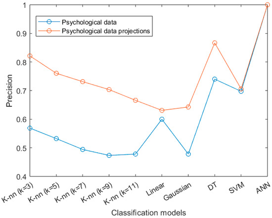
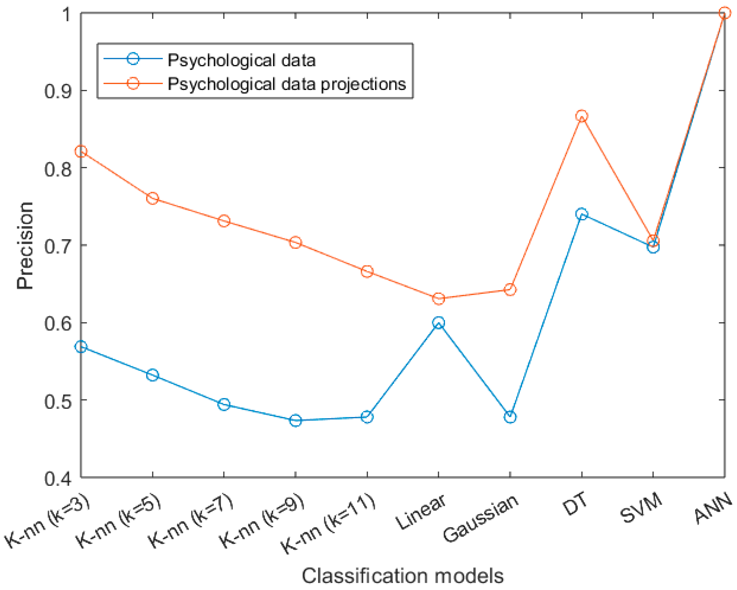
3.2.3. Performance Comparison: Raw vs. Projected Psychological Data

Figure 3 illustrates the comparative performance of the classification models when trained on raw psychological variables versus the optimized latent projections generated by the $DE-LD{A}_{FE}$ method. Consistent with the findings from the clinical dataset, the application of the $DE-LD{A}_{FE}$ method successfully enhanced class separability, contributing to a systematic improvement in classification metrics across K-nn, Linear, DT, and SVM.

The sole exception in this experimental phase was the ANN model. Because the dynamically configured ANN had already achieved perfect predictive accuracy (1.0000) using the raw psychological data, its performance metrics remained identical when processing the projected data, demonstrating a ceiling effect in its classification capability for this specific model.

3.3. Classification Based on Combined Clinical and Psychological Variables

3.3.1. Analysis of Raw Combined Data

In this comprehensive phase of the study, the classification models were evaluated using an integrated dataset comprising both the raw clinical and psychological variables. This experiment was designed to determine whether combining these two distinct domains, the biological risk factors and the psychological states, without any prior preprocessing or projection, enhances the overall predictive accuracy for breast cancer risk. The comparative performance metrics are presented in

Table 8. Performance metrics of classification models using raw combined clinical and psychological data.

Classification Model	TP RATE	FP RATE	Precision	Recall	F1-Score	AUC-ROC
K-nn (3)	0.6369	0.3998	0.7259	0.6404	0.6513	0.8510
K-nn (5)	0.6026	0.4145	0.6340	0.5432	0.5468	0.7579
K-nn (7)	0.6167	0.4562	0.5632	0.5015	0.4953	0.6959
K-nn (9)	0.5743	0.4556	0.4833	0.4237	0.4030	0.6510
K-nn (11)	0.5948	0.4882	0.4959	0.4327	0.4036	0.6378
Linear	0.7812	0.3623	0.7931	0.7762	0.7834	0.9227
Gaussian	0.0000	0.0000	0.0000	0.0000	0.0000	0.0000
DT	0.7215	0.3293	0.7770	0.7629	0.7679	0.9053
SVM	0.7958	0.3550	0.8929	0.8554	0.8693	0.9448
ANN (20)	0.8765	0.2249	1.0000	1.0000	1.0000	1.0000

Classification models: K-Nearest Neighbors (K-nn), Linear Discriminant Classifier (Linear), Gaussian Classifier (Gaussian), Decision Tree (DT), Support Vector Machine (SVM), Artificial Neural Network (ANN). The optimal ANN architecture comprises one hidden layer with 20 neurons per layer.

.

As detailed in Table 8, the ANN, configured with 20 neurons in its hidden layer, once again demonstrated exceptional predictive capacity on the raw data, achieving perfect scores in several key metrics (Precision: 1.0000; F1-score: 1.0000). The integration of both variable sets significantly improved the performance of the SVM model, which emerged as the second most robust classifier for this combined dataset (Precision: 0.8929; F1-score: 0.8693). Consistent with previous experimental phases, the K-nn model’s performance degraded progressively as the number of neighbors (K) increased, reaffirming that K = 3 remains the optimal parameter setting for this algorithm.

Intriguingly, the Gaussian classifier failed to converge valid predictions in this combined raw space (yielding 0.0000 across all metrics). This was further analyzed and is primarily attributed to the high dimensionality of the feature space relative to the number of samples. In this setting, the covariance matrix becomes ill-conditioned or singular, preventing its reliable inversion and leading to degenerate probability estimates, which explains the zero values observed across all evaluation metrics. This issue was verified by inspecting the rank and condition number of the covariance matrix. These findings further justify the use of dimensionality reduction methods, such as $DE-LD{A}_{FE}$, which project the data into a lower-dimensional space where covariance estimation is stable, and class separability is significantly improved.

3.3.2. Classification Using Combined Data Projections via the $DE-LD{A}_{FE}$ Method

To address the complexities of the combined dataset, the integrated clinical and psychological variables were projected into an optimized latent space using the $DE-LD{A}_{FE}$ method. Table 8 presents the average performance metrics of the classification models, calculated over 10 independent runs, when trained on these combined, optimized projections.

As shown in

Table 9. Projection results of the clinical and psychological variables obtained with the $DE-LD{A}_{FE}$ method.

Classification Model	TP RATE	FP RATE	Precision	Recall	F1-Score	AUC-ROC
K-nn (3)	0.7454	0.2736	0.8435	0.8384	0.8400	0.9586
K-nn (5)	0.7439	0.2578	0.7983	0.7700	0.7802	0.9375
K-nn (7)	0.7677	0.2751	0.7874	0.7724	0.7784	0.9236
K-nn (9)	0.7610	0.2798	0.7790	0.7701	0.7738	0.9208
K-nn (11)	0.7547	0.2924	0.7626	0.7544	0.7575	0.9188
Linear	0.7815	0.3621	0.7900	0.7716	0.7792	0.9232
Gaussian	0.7849	0.3604	0.7956	0.7817	0.7876	0.9283
DT	0.7620	0.3064	0.8874	0.8867	0.8853	0.9593
SVM	0.7830	0.3613	0.7880	0.7632	0.7723	0.9254
ANN (500)	0.9073	0.1451	0.9975	0.9977	0.9976	1.0000

Classification models: K-Nearest Neighbors (K-nn), Linear Discriminant Classifier (Linear), Gaussian Classifier (Gaussian), Decision Tree (DT), Support Vector Machine (SVM), Artificial Neural Network (ANN). The optimal ANN architecture comprises two hidden layers with 500 neurons per layer.

, the models demonstrating the highest predictive capability on the projected combined variables were the ANN, utilizing an expanded 500-neuron architecture, which achieved near-perfect average metrics (Precision: 0.9975; F1-score: 0.9976), followed by the DT model (Precision: 0.8874; F1-score: 0.8853).

Notably, the application of the $DE-LD{A}_{FE}$ method resolved the prior convergence failure of the Gaussian model on the raw combined data. By optimizing the dimensional space, the Gaussian algorithm successfully generated predictions, achieving a highly competitive Precision of 0.7956. Lastly, among the K-nn configurations, an increase in neighbors (K) again correlated with a decrease in Precision and F1-score, establishing again that K = 3 is the optimal baseline for this model.

Table 10. Best individual run performance for each classification model using combined data projections via $DE-LD{A}_{FE}$.

Classification Model	Experiment	TP RATE	FP RATE	Precision	Recall	F1-Score	AUC-ROC
K-nn (3)	1	0.7478	0.2748	0.8663	0.8630	0.8643	0.9636
K-nn (5)	4	0.7542	0.2528	0.8239	0.7956	0.8062	0.9459
K-nn (7)	2	0.7716	0.2723	0.8160	0.7847	0.7951	0.9276
K-nn (9)	9	0.7633	0.2759	0.8160	0.8052	0.8100	0.9277
K-nn (11)	2	0.7574	0.2941	0.7868	0.7705	0.7772	0.9220
Linear	2	0.7823	0.3616	0.8008	0.7853	0.7918	0.9246
Gaussian	6	0.7862	0.3598	0.8037	0.7924	0.7973	0.9303
DT	5	0.7783	0.2578	0.9148	0.9099	0.9077	0.9730
SVM	10	0.7842	0.3605	0.7991	0.7776	0.7860	0.9275
ANN (500)	3	0.8739	0.2205	1.0000	1.0000	1.0000	1.0000

Classification models: K-Nearest Neighbors (K-nn), Linear Discriminant Classifier (Linear), Gaussian Classifier (Gaussian), Decision Tree (DT), Support Vector Machine (SVM), Artificial Neural Network (ANN).

details the single best-performing run out of the 10 total executions for each model, highlighting the peak potential of these classifiers when utilizing the combined data projections.

The results in Table 10 mirror the trends observed in the average metrics, reinforcing the superiority of the ANN model, which achieved flawless classification (Precision: 1.0000; F1-score: 1.0000) during Experiment 3. The DT model similarly peaked during experiment 5, yielding an outstanding Precision of 0.9148 and an F1-score of 0.9077. The remaining algorithms exhibited consistent, high-tier performance, validating the efficacy of the $DE-LD{A}_{FE}$ transformation on combined, heterogeneous datasets. Once again, in the case of the K-nn model, as the number of neighbors (K) increases, both the Precision and the F1-score tend to decrease. Therefore, the value of K = 3 corresponds to the best performance within this configuration.

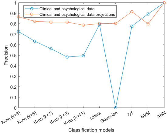
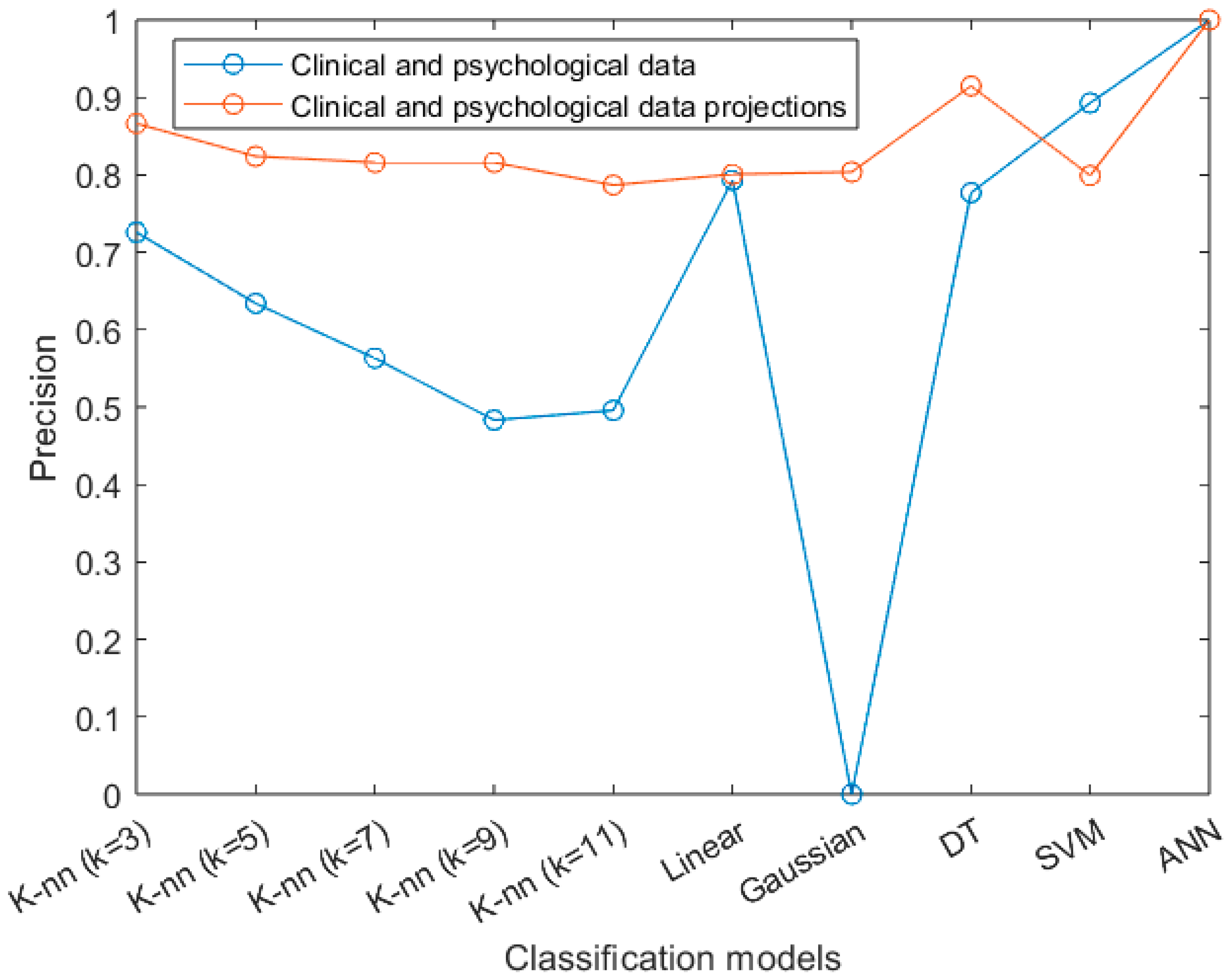
3.3.3. Performance Comparison: Raw vs. Projected Combined Data

Figure 4 illustrates the comparative performance of the classification models when trained on the raw, combined clinical and psychological dataset versus the optimized latent projections generated by the $DE-LD{A}_{FE}$ method. Consistent with the findings from the isolated datasets, the application of the $DE-LD{A}_{FE}$ method successfully enhanced class separability, contributing to improved classification metrics for K-nn, Linear, and DT models.

Two notable exceptions to this trend were the SVM and the ANN models, both of which achieved their peak performance utilizing the raw, unprojected data. As established in Section 3.3.1, the dynamically configured ANN had already reached perfect predictive accuracy (1.0000) on the raw combined data, while the SVM demonstrated a remarkably high natural affinity for delineating the raw integrated feature space.

In stark contrast, the Gaussian model benefited the most profoundly from the $DE-LD{A}_{FE}$ projections. While the algorithm completely failed to converge on the raw, heterogeneous data (yielding metrics of 0.0000), the optimized dimensionality reduction provided by the $DE-LD{A}_{FE}$ method resolved these mathematical singularities. This transformation allowed the Gaussian model to successfully compute probabilities and achieve highly competitive performance, underscoring the vital role of $DE-LD{A}_{FE}$ in stabilizing sensitive algorithms when integrating complex, multi-domain datasets.

3.4. Comprehensive Analysis of Variable Integration

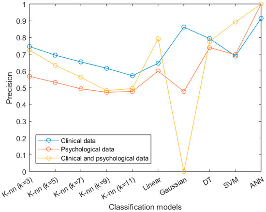
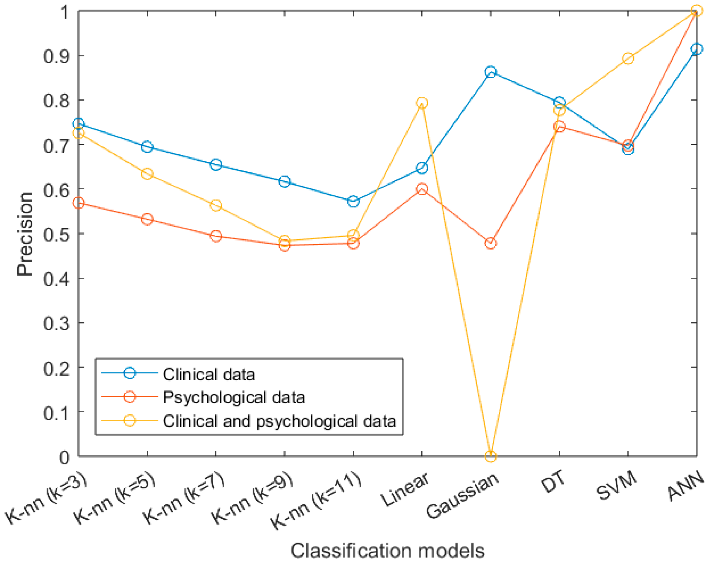
Figure 5 illustrates a comparative analysis of the precision achieved by the various classification models across the raw clinical, psychological, and integrated datasets. Across all unprojected data types, the ANN consistently demonstrated superior performance, achieving the highest precision and proving to be the best-performing architecture for this study’s baseline data.

Regarding the K-nn model, the analysis confirms that precision inversely correlates with the number of neighbors (K). The peak performance within this family of models was consistently observed at K = 3, particularly within the clinical and combined datasets, whereas higher K values systematically reduced the algorithm’s discriminative capacity. The Gaussian model performed adequately with isolated clinical and psychological data; however, it experienced a total convergence failure (precision dropping to zero) when attempting to process the raw combined variables, suggesting profound mathematical difficulty in handling this unprojected, heterogeneous data integration. The DT model exhibited robust and stable performance across all three data domains, standing out slightly on the clinical data with accuracy metrics superior to most baseline models, though not reaching the absolute ceiling of the ANN. Finally, the SVM and Linear maintained a generally intermediate performance profile, yielding acceptable precision without significantly outperforming the top-tier algorithms.

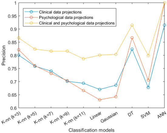
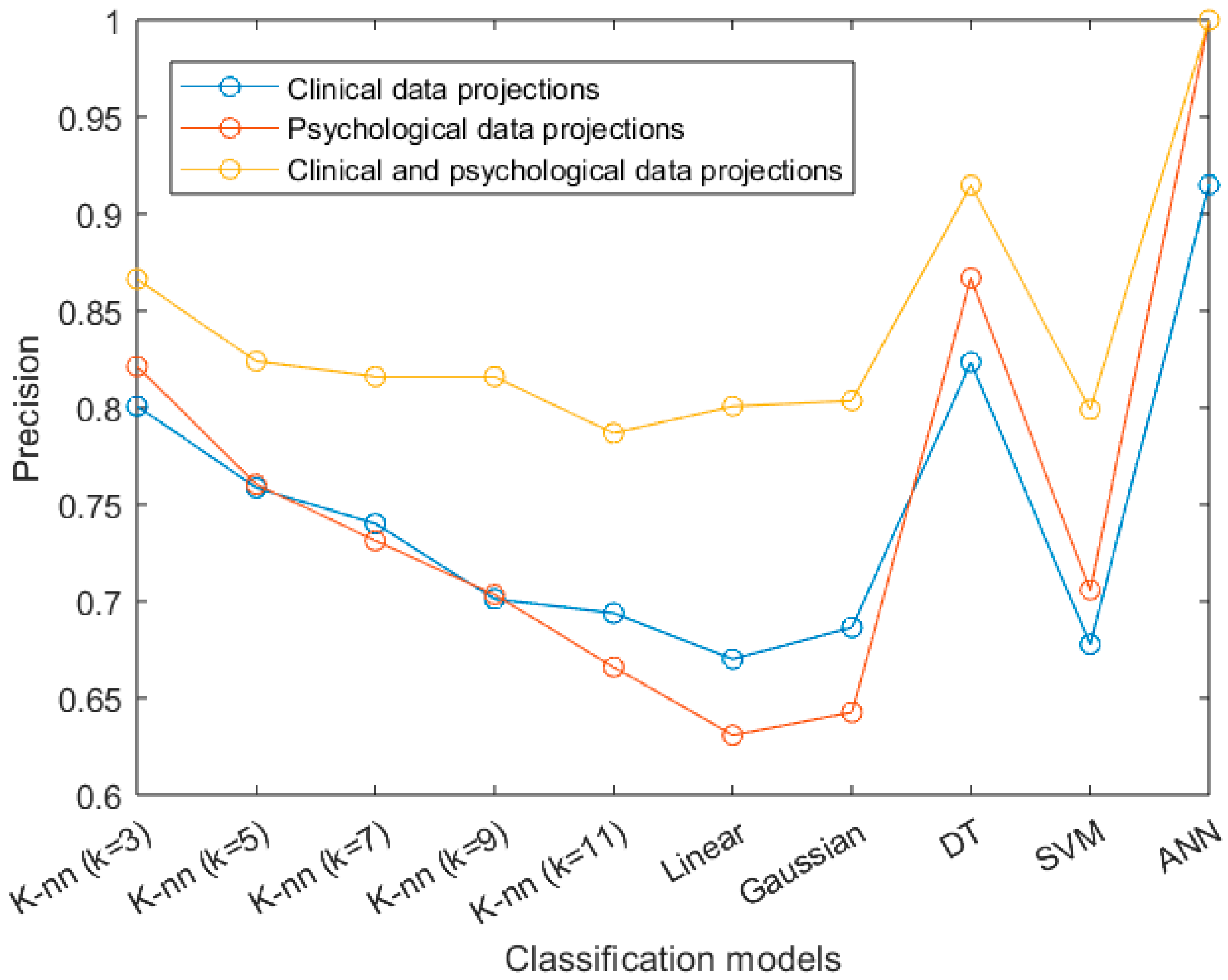
Figure 6 presents a parallel comparison of the models’ predictive accuracy when utilizing the optimized data projections (clinical, psychological, and combined) generated by the $DE-LD{A}_{FE}$ method. Significantly, the data indicates that the integration of both clinical and psychological variables into a combined, projected latent space yields the highest precision values across the majority of the evaluated models. This outcome strongly suggests that the complementary information derived from pairing biological risk factors with psychological states, when properly optimized and mathematically smoothed via the $DE-LD{A}_{FE}$ method, significantly enhances the overall discriminatory power and predictive reliability of the classifiers.

While the main objective of this work is to use clinical, psychological, and combined data to construct a breast cancer risk profile, it is also possible to identify, using the DE-LDA_FE method, isolated characteristics of each data type that may contribute to risk prediction. This is achieved through the use of a linear model, whose transformation matrix provides coefficients that reflect the relevance of the variables, ordered in descending order. The variables considered relevant are presented in Appendix B (

Table A4. Clinical and psychological data.

Variable	Coefficient
EPP	0.17075
Toxi	0.14542
gesta	0.13314
TR	0.12534
DH	0.098024
SG	0.092286
ANL	0.072743
RDL	0.066021
AH	0.065688
abo	0.062628

,

Table A5. Clinical Data.

Variable	Coefficient
EPP	0.17075
Toxi	0.14542
gesta	0.13314
TRH	0.12534
abo	0.062628

and

Table A6. Psychological data.

Variable	Coefficient
DH	0.098024
SGL	0.092286
ANL	0.072743
RDL	0.066021
AH	0.065688

). However, as noted by Montes-Nogueira et al. (2018) and Romo-Gonzalez et al. (2018) [11,12], the breast cancer risk profile is more robust when clinical and psychological data are integrated together, rather than using isolated characteristics.

4. Discussion

4.1. The Need for Context-Specific Risk Models

Breast cancer remains one of the most critical public health issues globally, disproportionately affecting women in developing countries such as Mexico. Despite advancements in diagnosis and treatment, mortality rates remain high, largely due to delayed detection and the limited reach of effective screening programs. In Mexico, breast cancer has become the leading cause of cancer-related deaths among women, and its clinical presentation occurs approximately a decade earlier than in high-income countries. These circumstances highlight the urgent need for early detection tools adapted to the specific characteristics of the Mexican population.

Several models have been designed to evaluate the risk of developing breast cancer throughout a woman’s life. The most widely used—such as the Breast Cancer Risk Assessment Tool (Gail Model), the International Breast Cancer Intervention Study (Tyrer-Cuzick Model), and the Breast and Ovarian Analysis of Disease Incidence and Carrier Estimation Algorithm (BOADICEA)—rely on biological and reproductive risk data to provide estimates that guide physician decisions regarding future screening, preventive interventions, or chemoprophylaxis [35,36]. While these tools have proven their efficacy and are widely used in developed countries [37], they rely primarily on biological metrics, failing to account for the complex sociocultural or psychological dimensions that are critical in other demographic groups.

Currently, Mexico lacks risk-assessment tools calibrated to the national population that consider lifestyle or psychological factors. Consequently, these standardized models may lack predictive power when applied to Mexican women, who experience different environmental stressors, cultural pressures, and emotional coping strategies than the populations for which the models were originally developed. Our baseline results support this limitation: the clinical-only models failed to distinguish accurately between benign pathology and cancer, suggesting that biological risk factors overlap significantly between these groups. It was only the addition of psychological profiling that successfully “unlocked” the models’ discriminative power.

4.2. Model Performance and the “Black Box” Problem

Our results demonstrate that integrating psychological variables—specifically emotional repression, suppression, and stress symptoms—with standard clinical history significantly enhances breast cancer risk prediction. The classification models achieved their greatest accuracy when utilizing the combined projections of clinical and psychological variables optimized through the $DE-LD{A}_{FE}$ method (Precision: 0.8874–0.9975; F1-score: 0.8853–0.9976), far outperforming the individual, not projected datasets.

Across the evaluated algorithms, the ANN clearly stood out as the most accurate model, reaching its peak when clinical and psychological variables were combined. However, while the ANN achieved the highest accuracy metrics, its complex architecture renders it a “black box.” This limits the interpretability of the results, which is a critical issue in the medical field where understanding how a given prediction is reached is essential for clinical trust and patient communication. This issue of explainability has been highlighted in the recent literature [38], emphasizing the need for using Explainable Artificial Intelligence (XAI) in healthcare. Consequently, as our work points out, the DT model, which ranked second in overall performance, appears to be a more suitable and practical alternative for medical applications. It allows clinicians to visually track the classification process and transparently explain the specific criteria used to arrive at a risk assessment.

4.3. Psychological Variables and Physiological Pathways

The empirical evidence generated by our models supports the hypothesis that psychological factors are not merely incidental comorbidities, but rather associated risk factors in the multidimensional etiology of breast cancer. The predictive value of psychological variables aligns closely with Type C Personality Theory [15,16,17]. Our data suggest that high levels of emotional suppression (measured by the CECS) and defensiveness (measured by the WAI) could be related as distinctive markers in the breast cancer group.

Physiologically, the relationship of these traits within the multicausal etiology of the disease could be explained by established psychoneuroimmunological mechanisms. That is, chronic emotional inhibition is known to dysregulate the hypothalamic–pituitary–adrenal axis, altering cortisol secretion patterns. This dysregulation could, in turn, affect immune surveillance and tumor suppression mechanisms [11,13,14]. Therefore, the greater accuracy achieved by combining psychological and clinical data indicates that emotional suppression and distress symptoms are not only consequences of the disease but could also serve as early indicators of physiological vulnerability.

4.4. Clinical Implications and Future Applications

The proposed $DE-LD{A}_{FE}$ algorithmic pipeline offers a scalable, non-invasive alternative for early screening. Unlike standard mammography, which is resource-intensive and carries radiation risks, this methodology could be deployed as a web-based or mobile pre-screening module. Such a tool would be particularly valuable in low-resource settings, offering the following systemic benefits:

(a) Empowering Patients: Providing women with access to validated self-assessment tools in contexts where direct medical services may be limited or geographically inaccessible.

(b) Optimizing Triage: enabling primary care providers to prioritize referrals for women who exhibit a high-risk biopsychosocial profile, even if they are young or asymptomatic.

This module could be readily adapted for broader use across Latin America, significantly enhancing early detection frameworks in resource-constrained areas.

4.5. Limitations/Future Work

While the results are very promising, this study has limitations that should guide future research. First, the sample size (n = 110), although statistically sufficient for this exploratory validation, requires further expansion. Future studies should incorporate a larger multicenter cohort to ensure the model’s generalizability across the diverse geographic and socioeconomic regions of Mexico. They should also incorporate techniques for handling missing data and unbalanced cohorts. Although the proposed algorithm successfully separates risk groups, the cross-sectional nature of the data limits definitive causal inference. Longitudinal studies are needed to confirm whether these specific psychological traits precede cellular malignancy or evolve concurrently with it. Reference methods such as entropy-regulated two-view NMF and semi-supervised adaptive symmetric NMF could also be applied, as they offer comparative frameworks and could reveal how the observed benefits behave under more diverse age distributions, patterns of missing data, or larger-scale multicenter cohorts. In-depth sensitivity and robustness analyses should also be performed on the experiments.

5. Conclusions

This study provides strong empirical support of the biopsychosocial model in oncology. It demonstrates that combining engineered clinical and psychological features via the $DE-LD{A}_{FE}$ projection method significantly enhances the discriminative power of machine learning classifiers. Ultimately, this research illustrates that Artificial Intelligence can effectively bridge the gap between psychology and biological oncology, offering a powerful, context-specific, and non-invasive tool to address the rising burden of BC in Mexico.

References

- World Health Organization. Data Visualization Tools for Exploring the Global Cancer Burden in 2022; Cancer Today; World Health Organization: Geneva, Switzerland, 2024. [Google Scholar]
- Maffuz-Aziz, A.; Labastida-Almendaro, S.; Espejo-Fonseca, A.; Rodríguez-Cuevas, S. Características clinicopatológicas del cáncer de mama en una población de mujeres en México. Cirugía Cir. 2017, 85, 201–207. [Google Scholar] [CrossRef] [Scilit]
- Cárdenas-Sánchez, J. Consenso mexicano sobre diagnóstico y tratamiento del cáncer mamario. Mex. J. Oncol. 2022, 20, 6923. [Google Scholar] [CrossRef] [Scilit]
- Díaz Godinez, M.M. Estadísticas a Propósito del Día Internacional de la Lucha Contra el Cáncer de Mama (19 de Octubre); INEGI: Aguascalientes, Mexico, 2023. [Google Scholar]
- Seimenis, I.; Chouchos, K.; Prassopoulos, P. Radiation Risk Associated with X-Ray Mammography Screening: Communication and Exchange of Information via Tweets. J. Am. Coll. Radiol. 2018, 15, 1033–1039. [Google Scholar] [CrossRef] [Scilit] [PubMed]
- Di Maria, S.; Van Nijnatten, T.J.A.; Jeukens, C.R.L.P.N.; Vedantham, S.; Dietzel, M.; Vaz, P. Understanding the Risk of Ionizing Radiation in Breast Imaging: Concepts and Quantities, Clinical Importance, and Future Directions. Eur. J. Radiol. 2024, 181, 111784. [Google Scholar] [CrossRef] [Scilit]
- Chaudhary, L.; Knapp, S.; Wen, S.; Xiao, J.; Marano, G.; Kurian, S.; Layne, G.; Jacobson, G.; Abraham, J. Radiation Exposure from Diagnostic Procedures in Patients with Newly Diagnosed Breast Cancer. J. Community Support. Oncol. 2015, 13, 27–29. [Google Scholar] [CrossRef] [Scilit]
- Chávarri-Guerra, Y.; Villarreal-Garza, C.; Liedke, P.E.; Knaul, F.; Mohar, A.; Finkelstein, D.M.; Goss, P.E. Breast Cancer in Mexico: A Growing Challenge to Health and the Health System. Lancet Oncol. 2012, 13, e335–e343. [Google Scholar] [CrossRef] [Scilit] [PubMed]
- Villarreal-Garza, C.; Platas, A.; Miaja, M.; Fonseca, A.; Mesa-Chavez, F.; Garcia-Garcia, M.; Chapman, J.-A.; Lopez-Martinez, E.A.; Pineda, C.; Mohar, A.; et al. Young Women with Breast Cancer in Mexico: Results of the Pilot Phase of the Joven & Fuerte Prospective Cohort. JCO Glob. Oncol. 2020, 6, 395–406. [Google Scholar] [CrossRef] [Scilit] [PubMed]
- Avila, M.H. NORMA Oficial Mexicana NOM-041-SSA2-2011, Para la Prevención, Diagnóstico, Tratamiento, Control y Vigilancia Epidemiológica del Cáncer de Mama; Diario Oficial de la Federación: CDMX, México, 2011. [Google Scholar]
- Romo-González, T.; Martínez, A.J.; Hernández-Pozo, M.D.R.; Gutiérrez-Ospina, G.; Larralde, C. Psychological Features of Breast Cancer in Mexican Women I: Personality Traits and Stress Symptoms. Adv. Neuroimmune Biol. 2018, 7, 3–15. [Google Scholar] [CrossRef] [Scilit]
- Montes-Nogueira, I.; Campos-Uscanga, Y.; Gutiérrez-Ospina, G.; Hernández-Pozo, M.D.R.; Larralde, C.; Romo-González, T. Psychological Features of Breast Cancer in Mexican Women II: The Psychological Network. Adv. Neuroimmune Biol. 2018, 7, 91–105. [Google Scholar] [CrossRef] [Scilit]
- Giese-Davis, J.; Wilhelm, F.H.; Conrad, A.; Abercrombie, H.C.; Sephton, S.; Yutsis, M.; Neri, E.; Taylor, C.B.; Kraemer, H.C.; Spiegel, D. Depression and Stress Reactivity in Metastatic Breast Cancer. Psychosom. Med. 2006, 68, 675–683. [Google Scholar] [CrossRef] [Scilit]
- Giese-Davis, J.; Koopman, C.; Butler, L.D.; Classen, C.; Cordova, M.; Fobair, P.; Benson, J.; Kraemer, H.C.; Spiegel, D. Change in Emotion-Regulation Strategy for Women with Metastatic Breast Cancer Following Supportive-Expressive Group Therapy. J. Consult. Clin. Psychol. 2002, 70, 916–925. [Google Scholar] [CrossRef]
- Greer, S.; Morris, T. Psychological Attributes of Women Who Develop Breast Cancer: A Controlled Study. J. Psychosom. Res. 1975, 19, 147–153. [Google Scholar] [CrossRef] [Scilit]
- Temoshok, L. Personality, Coping Style, Emotion and Cancer: Towards an Integrative Model. Cancer Surv. 1987, 6, 545–567. [Google Scholar]
- Iwamitsu, Y.; Shimoda, K.; Abe, H.; Tani, T.; Kodama, M.; Okawa, M. Differences in Emotional Distress between Breast Tumor Patients with Emotional Inhibition and Those with Emotional Expression. Psychiatry Clin. Neurosci. 2003, 57, 289–294. [Google Scholar] [CrossRef] [Scilit] [PubMed]
- Myers, L.B. The Importance of the Repressive Coping Style: Findings from 30 Years of Research. Anxiety Stress Coping 2010, 23, 3–17. [Google Scholar] [CrossRef] [Scilit] [PubMed]
- McGregor, B.A.; Antoni, M.H. Psychological Intervention and Health Outcomes among Women Treated for Breast Cancer: A Review of Stress Pathways and Biological Mediators. Brain Behav. Immun. 2009, 23, 159–166. [Google Scholar] [CrossRef] [Scilit] [PubMed]
- García Camacho, A. Módulo Web Para la Obtencion de Riesgo de Padecer Cáncer de Mama Mediante Datos Psicológicos y Clínicos. Bachelor’s Thesis, Universidad Veracruzana, Xalapa, Ver., Mexico, 2017. [Google Scholar]
- Hussain, S.; Ali, M.; Naseem, U.; Nezhadmoghadam, F.; Jatoi, M.A.; Gulliver, T.A.; Tamez-Peña, J.G. Breast Cancer Risk Prediction Using Machine Learning: A Systematic Review. Front. Oncol. 2024, 14, 1343627. [Google Scholar] [CrossRef] [Scilit]
- Geißler, K.; Koller, T.L.; Ambroladze, A.; Fallenberg, E.M.; Ingrisch, M.; Hahn, H.K. Breast Cancer Risk Prediction Using Background Parenchymal Enhancement, Radiomics, and Symmetry Features on MRI. In Proceedings of the Medical Imaging 2025: Computer-Aided Diagnosis; SPIE: Cergy-Pontoise, France, 2025; Volume 13407, pp. 564–568. [Google Scholar]
- Wang, J.; Zhang, Z.; Wang, Y. Utilizing Feature Selection Techniques for AI-Driven Tumor Subtype Classification: Enhancing Precision in Cancer Diagnostics. Biomolecules 2025, 15, 81. [Google Scholar] [CrossRef] [Scilit]
- Carriero, A.; De Hond, A.; Cappers, B.; Paulovich, F.; Abeln, S.; Moons, K.G.; Van Smeden, M. Explainable AI in Healthcare: To Explain, to Predict, or to Describe? Diagn. Progn. Res. 2025, 9, 29. [Google Scholar] [CrossRef] [Scilit]
- Berahmand, K.; Zhou, X.; Li, Y.; Gururajan, R.; Barua, P.D.; Acharya, U.R.; Chennakesavan, S.K. NEDL-GCP: A Nested Ensemble Deep Learning Model for Gynecological Cancer Risk Prediction. Array 2025, 27, 100468. [Google Scholar] [CrossRef] [Scilit]
- Doumari, S.A.; Berahmand, K.; Ebadi, M.J. Early and High-Accuracy Diagnosis of Parkinson’s Disease: Outcomes of a New Model. Comput. Math. Methods Med. 2023, 2023, 1493676. [Google Scholar] [CrossRef] [Scilit]
- Romo-González, T.; Barranca-Enríquez, A.; León-Díaz, R.; Del Callejo-Canal, E.; Gutiérrez-Ospina, G.; Jimenez Urrego, A.M.; Bolaños, C.; Botero Carvajal, A. Psychological Suppressive Profile and Autoantibodies Variability in Women Living with Breast Cancer: A Prospective Cross-Sectional Study. Heliyon 2022, 8, e10883. [Google Scholar] [CrossRef] [Scilit]
- Benevides-Pereira, A.M.T.; Moreno-Jiménez, B.; Garrosa Hernández, E.; González Gutiérrez, J.L. La evaluación específica del síndrome de burnout en psicólogos: El Inventario de burnout de psicólogos. Clínica Salud 2002, 13, 257–283. [Google Scholar]
- Watson, M.; Greer, S. Development of a Questionnaire Measure of Emotional Control. J. Psychosom. Res. 1983, 27, 299–305. [Google Scholar] [CrossRef] [Scilit] [PubMed]
- Durá, E.; Andreu, Y.; Galdón, M.J.; Ibáñez, E.; Pérez, S.; Ferrando, M.; Murgui, S.; Martínez, P. Emotional Suppression and Breast Cancer: Validation Research on the Spanish Adaptation of the Courtauld Emotional Control Scale (CECS). Span. J. Psychol. 2010, 13, 406–417. [Google Scholar] [CrossRef] [Scilit]
- Weinberger, D.A. The Construct Validity of the Repressive Coping Style. In Repression and Dissociation: Implications for Personality Theory, Psychopathology and Health; Singer, J.L., Ed.; University of Chicago Press: Chicago, IL, USA, 1990; pp. 337–386. [Google Scholar]
- Weinberger, D.A.; Schwartz, G.E. Distress and Restraint as Superordinate Dimensions of Self-Reported Adjustment: A Typological Perspective. J. Personal. 1990, 58, 381–417. [Google Scholar] [CrossRef] [Scilit]
- Weinberger, D.A. Distress and Self-Restraint as Measures of Adjustment across the Life Span: Confirmatory Factor Analyses in Clinical and Nonclinical Samples. Psychol. Assess. 1997, 9, 132–135. [Google Scholar] [CrossRef]
- Romo González, T.; Enríquez-Hernández, C.B.; Hernández Pozo, M.D.R.; Ruiz Montalvo, M.E.; Castillo, R.L.; Ehrenzweig Sánchez, Y.; Marván, M.L.; Larralde, C. Validación en México del inventario de ajuste de Weinberger (WAI). Salud Ment. 2014, 37, 247. [Google Scholar] [CrossRef] [Scilit]
- Amir, N.; Beard, C.; Burns, M.; Bomyea, J. Attention Modification Program in Individuals with Generalized Anxiety Disorder. J. Abnorm. Psychol. 2009, 118, 28–33. [Google Scholar] [CrossRef] [Scilit]
- Brentnall, A.R.; Harkness, E.F.; Astley, S.M.; Donnelly, L.S.; Stavrinos, P.; Sampson, S.; Fox, L.; Sergeant, J.C.; Harvie, M.N.; Wilson, M.; et al. Mammographic Density Adds Accuracy to Both the Tyrer-Cuzick and Gail Breast Cancer Risk Models in a Prospective UK Screening Cohort. Breast Cancer Res. 2015, 17, 147. [Google Scholar] [CrossRef] [Scilit] [PubMed]
- Terry, M.B.; Liao, Y.; Whittemore, A.S.; Leoce, N.; Buchsbaum, R.; Zeinomar, N.; Dite, G.S.; Chung, W.K.; Knight, J.A.; Southey, M.C.; et al. 10-Year Performance of Four Models of Breast Cancer Risk: A Validation Study. Lancet Oncol. 2019, 20, 504–517. [Google Scholar] [CrossRef] [Scilit] [PubMed]
- Hassija, V.; Chamola, V.; Mahapatra, A.; Singal, A.; Goel, D.; Huang, K.; Scardapane, S.; Spinelli, I.; Mahmud, M.; Hussain, A. Interpreting Black-Box Models: A Review on Explainable Artificial Intelligence. Cogn. Comput. 2024, 16, 45–74. [Google Scholar] [CrossRef] [Scilit]
Disclaimer/Publisher’s Note: The statements, opinions and data contained in all publications are solely those of the individual author(s) and contributor(s) and not of MDPI and/or the editor(s). MDPI and/or the editor(s) disclaim responsibility for any injury to people or property resulting from any ideas, methods, instructions or products referred to in the content. |
© 2026 by the authors. Licensee MDPI, Basel, Switzerland. This article is an open access article distributed under the terms and conditions of the Creative Commons Attribution (CC BY) license.