Neuroevolution of Liquid State Machine Based on Neural Configurations and Positions

Abstract

Liquid State Machines (LSMs), a reservoir computing model based on recurrent spiking neural networks, provide a powerful framework for solving spatiotemporal classification tasks by leveraging rich temporal dynamics and event-driven processing. Although the traditional LSM formulation assumes a fixed, randomly generated reservoir, recent research has explored optimization strategies to improve liquid dynamics. However, most existing approaches focus primarily on optimizing synaptic connectivity or reservoir structure, while the role of neuron-level parameters remains largely underexplored. This work proposes a neuroevolutionary strategy based on a Genetic Algorithm (GA) that encodes both neuron configurations and their spatial positions, explicitly treating neuron-level parameters as optimization targets. By evolving neuron-specific parameters and spatial positions, the method induces diverse reservoir dynamics. Unlike approaches that directly optimize synaptic weights, the proposed representation maintains an encoding whose dimensionality scales linearly with the number of neurons. The approach was evaluated on four synthetic benchmark tasks, including one Frequency Recognition task and three Pattern Recognition tasks, using compact reservoirs composed of only 20 Leaky Integrate-and-Fire neurons. Despite the small reservoir size, the method achieved state-of-the-art or highly competitive performance, reaching mean accuracies of up to 99.71%. In the most challenging case (PR12), performance improved when the reservoir size was increased to 64 neurons. The method was further evaluated on two real-world datasets, N-MNIST and the Free Spoken Digit Dataset (FSDD), using reservoirs of 300 neurons, achieving 90.65% and 81.47% accuracy, respectively, while using substantially fewer neurons than many existing LSM-based approaches. These results highlight the potential of evolving neuron configurations and spatial organization to produce compact and effective liquid reservoirs.

1. Introduction

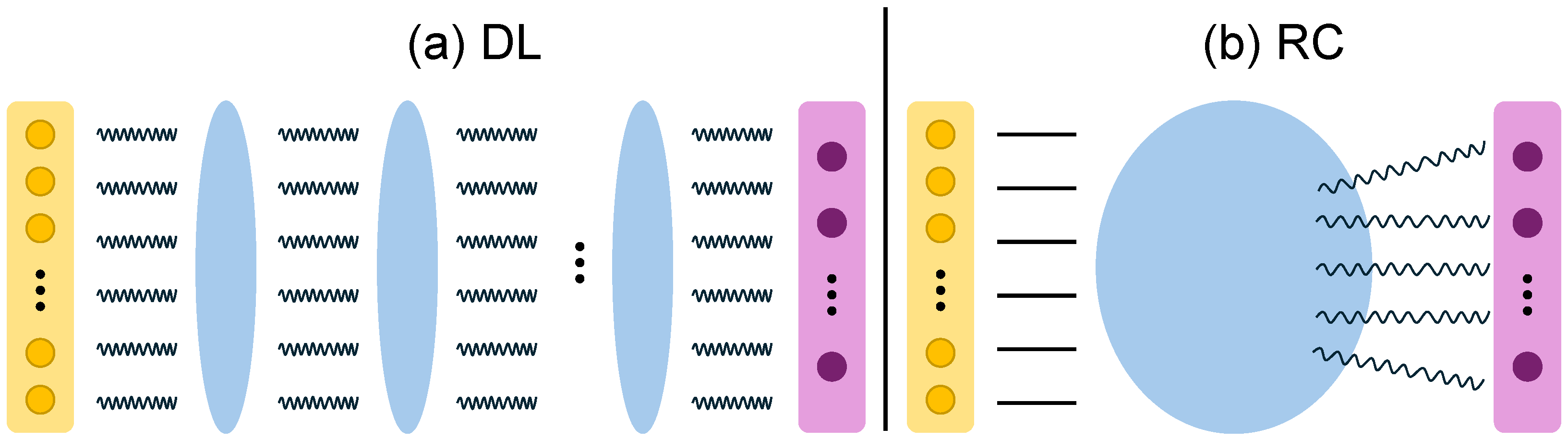
Reservoir Computing (RC) is an emerging machine-learning paradigm that originated in the early 2000s [1] and leverages high-dimensional dynamical systems (reservoirs) for nonlinear transformations [2] to learn spatiotemporal features and patterns in complex time series [3]. It is built on three levels: an Input layer, a Reservoir layer, and a Readout layer. The Input layer maps the input data into the reservoir via sparse, randomly weighted connections [4]. It is responsible for preprocessing data and ensuring that incoming signals activate the reservoir properly [5]. The Reservoir layer is the computational core of this model, as it is responsible for transforming the input into a high-dimensional representation, also referred to as states, where complex patterns and relationships are more easily discernible [6]. It comprises many interconnected neurons (computational units) with fixed-weight synapses (or connections). By this definition, the reservoir can be considered a type of Artificial Neural Network (ANN), specifically a Recurrent Neural Network (RNN), which allows the reservoir to preserve historical information [2]. Finally, the Readout layer serves as the output segment of the model, mapping the states produced by the Reservoir layer into a lower number of desired outputs [6]. Typically, a simple linear model, such as the Perceptron [7], is sufficient as a Readout function, and this is the only part of the model that requires a training process, which makes the RC a highly computationally efficient approach [8] when compared with Deep Learning (DL) algorithms. This is depicted in Figure 1.

Historically, two main RC representatives have been independently developed: the Echo State Network (ESN) [4] and the Liquid State Machine (LSM) [2]. The principal difference between them is that ESN uses a traditional RNN as a reservoir, where the neurons are continuous-valued units with traditional activation functions, such as the Rectified Linear Unit (ReLU). In contrast, LSM uses reservoirs, often referred to in this context as Liquids, of Recurrent Spiking Neural Networks (R-SNN) with biologically inspired spiking neurons. While ESN effectively models continuous-valued temporal signals, LSM enables precise spike timing and millisecond-scale temporal resolution. Moreover, experimental comparisons have shown that the performance of reservoir computing models depends strongly on reservoir dynamics and connectivity [9].

Although deep recurrent architectures such as Long Short-Term Memory (LSTM), Gated Recurrent Unit (GRU), and Transformer-based models have achieved remarkable performance on temporal tasks, they require full backpropagation through time, large labeled datasets, and substantial computational resources. In contrast, LSMs decouple the nonlinear temporal representation (reservoir) from the learning process (readout), thereby enabling efficient training while preserving rich dynamical representations and reducing computational cost [10]. Moreover, when dealing with event-based or spike-driven data, spiking reservoirs naturally preserve temporal precision without requiring continuous-valued approximations, making LSMs suitable for resource-constrained environments, such as embedded systems, edge devices, and neuromorphic hardware platforms, where memory capacity, energy consumption, and processing power are limited [11,12]. Therefore, rather than competing directly with fully trained deep architectures, this work focuses on enhancing the internal dynamics of LSM reservoirs to improve performance while preserving computational efficiency.

Spiking neuron models aim to capture the temporal dynamics of biological neurons by representing information through discrete spikes. Among the models proposed in the literature, the Hodgkin–Huxley model [13] provides a detailed biophysical description of neuronal activity but requires significant computational resources. For this reason, simplified models such as the Leaky Integrate-and-Fire (LIF) [14] neuron are commonly used in large-scale simulations, as they preserve the essential temporal dynamics while maintaining computational efficiency. In this work, we adopt the LIF model implemented in the NEST simulator [15].

Despite the LIF model’s simplicity, which makes it less plausible, its neuron parameters can encapsulate different temporal dynamics. In turn, this contributes to the proficiency of LSM in several areas, such as speech recognition [16,17,18], image and vision recognition [19,20,21], biomedical applications [22], robotics and control [23,24], among others. The possibility of avoiding explicit training is especially advantageous when using LSM since the synaptic plasticity mechanisms of R-SNNs require complex and computationally demanding training algorithms [25,26,27].

Since their formal introduction, LSMs have been associated with two cardinal attributes: the Separation Property (SP) and the Approximation Property (AP). In the context of classification tasks, SP measures the liquid’s ability to distinguish inputs belonging to different classes, whereas AP relates to the similarities in the liquid’s representation of two inputs belonging to the same class [28]; in other words, SP ensures that different inputs produce different liquid states and AP ensures that similar inputs produce similar liquid states.

Both of these metrics depend, to different degrees, on the internal complexity and dynamics of the liquid; consequently, the overall performance of an LMS is strongly influenced by its reservoir configuration. In its original formulation, Maass et al. [23] proposed that a randomly generated liquid would suffice to achieve adequate performance for a given task. That is, classical LSMs assume a fixed, untrained reservoir. However, this approach does not offer any solid support or assurance for complex tasks.

Later, Norton & Ventura [29,30,31] introduced an unsupervised adaptation mechanism known as Separation Driven Synaptic Modification (SDSM). Their method iteratively improves the SP by modifying synaptic weights using Hebbian Learning, while keeping the neuron model and parameters unchanged. This approximation introduces a form of reservoir training that remains unsupervised and self-organized. They tested their implementation using synthetic datasets proposed as frequency and pattern recognition tasks.

In contrast, recent approaches treat the liquid not as a fixed reservoir but as a trainable R-SNN, thereby relaxing the canonical LSM definition. This relaxation enables the enhancement of the liquid either through training-adaptation processes or by optimization techniques. Notably, R-SNNs have been successfully applied to temporal pattern recognition and decision-making tasks using learning rules such as Spike-Time Dependent Plasticity (STDP) and surrogate gradient methods [26,27,32,33]. However, these approaches typically involve computationally expensive training processes and require careful parameter tuning, which limits their scalability and practical applicability.

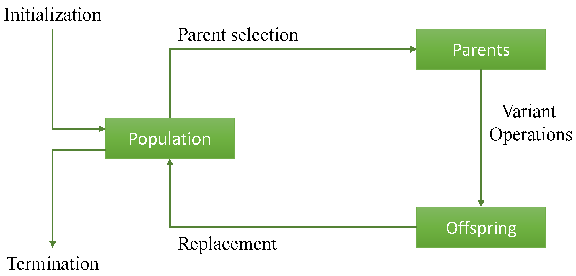
Among optimization strategies, metaheuristics such as Evolutionary Computation (EC) have shown promising results. EC encompasses various subfields, with Evolutionary Algorithms (EAs) and Swarm Intelligence (SI) algorithms being two of the most prominent. Generally, these methods take a set of potential solutions (or individuals) for a given problem, where a fitness function measures the aptitude of each individual. This way, the individuals are ranked according to a criterion. Therefore, through this competition, individuals are combined, eliminated, and substituted by new ones in every execution (generation or epoch) of the algorithm. Figure 2 depicts the general elements that most EA techniques follow. These algorithms are well-suited to LSM and R-SNN optimization due to their ability to explore high-dimensional spaces without relying on gradient information [32].

Moreover, Neuroevolution (NE) utilizes EC methods to optimize ANNs by searching the space of potential solutions of architectures and other parameters, such as weights [35], for a given task. Yaqoob & Wróbel [36] used a Genetic Algorithm (GA) to optimize the weights and connections in an R-SNN. The task was to detect a temporal pattern in the form of consecutive symbols in a continuous input stream. To achieve this, each symbol generated a temporal activation, delivered by the input neurons, that was then propagated throughout the rest of the network. They found that very small SNNs (with only a few neurons) could accurately recognize the pattern. As a neural model, they used AdEx neurons, an adaptation of the LIF model, with fixed parameters. Although the representation allowed for unlimited connections and nodes, it limited the number of interneurons to two.

Recent research has explored hierarchical extensions of reservoir computing, where multiple reservoirs are stacked to increase representational capacity [37]. Tian et al. [38] proposed an NE framework for designing a Multi-Liquid State Machine (MLSM); different liquids are disposed of in a layer-like structure. The authors propose a three-stage search strategy: first, a random architecture is optimized by moving liquids from one layer to another. Second, the number of neurons in each liquid of the LSM of the past stage is optimized while preserving the total number of neurons. Third, the framework optimizes the liquids’ internal parameters of the last LSM, such as the percentage of connectivity and excitatory neuron ratio. Each optimization step uses a Simulated Annealing (SA) algorithm. The framework is evaluated on two real-world benchmark datasets: the image dataset N-MNIST and the Free Spoken Digit Dataset (FSDD). The results show that the proposed framework can effectively search for high-performance LSM architectures while reducing the computational cost compared to manual search. Nevertheless, they rely on a complex structure comprised of 1000 spiking neurons and only consider connectivity in a limited manner (e.g., as a connectivity percentage), without exploring neuron configurations.

Zhou et al. [39] presented a framework named Generative Liquid State Machine (GLSM). The paper proposes a Cooperative Co-Evolutionary (CCE) algorithm for designing the reservoir architecture of LSMs using a Random Forest Surrogate (RFS) model. The algorithm treats the reservoir as a modular structure comprising subnetworks, utilizing the RFS model to minimize the computational cost of evaluating candidate architectures. A GA is used to evolve structures, the number of neurons, neuron thresholds, and neuron delays, while a learning algorithm is used to modify synaptic weights and delays. The results demonstrate that the proposed method effectively optimizes the LSM reservoir architecture. Nevertheless, this approach contemplates a fixed set of subnetworks and sub-reservoir configurations, limiting the neuron’s possibilities. Although they optimize the number of neurons, the exact number used in their implementations is not clearly specified. Modular GLSM-based reservoirs have also been explored for multi-task learning [40], where shared reservoir structures are used to address multiple tasks within a single framework.

Most recently, Alvarez-Canchila et al. [41] employed Particle Swarm Optimization (PSO), an SI approach, to optimize the SP. Each particle (solution) contained the synaptic weights of all connections in a liquid built with 64 neurons, predefined before every PSO run. They test it using the same tasks as Norton & Ventura [31], achieving accuracy levels comparable to those reported previously.

In summary, LSMs present several advantages for spatiotemporal learning tasks compared to conventional machine learning models. Their event-driven computation allows neurons to process information only when spikes occur [2,3], thereby reducing unnecessary operations and making them particularly suitable for implementation on neuromorphic hardware, where energy consumption can be significantly lower than in traditional deep learning architectures [11,12]. Moreover, the reservoir computing paradigm simplifies training by decoupling the dynamic transformation performed by the reservoir from the learning stage performed by the readout [3,10]. However, most works focus primarily on optimizing synaptic weights [31,41] or on predefined architectural structures [38,39], while neuron configuration and neuron positions in the liquid have received limited attention. In particular:

• Weight-based optimization methods (PSO, GA over synapses) assume a fixed neuron model and topology.
• Multi-liquid approaches optimize macro-architecture but do not explore intra-liquid neuronal diversity.
• Modular approaches constrain the search space to predefined substructures.

Consequently, the joint optimization of neuron configurations and spatial positions remains unexplored.

In this work, a GA method is proposed as an NE approach to optimize liquid performance. The decision to employ a GA is based on its simplicity, proven effectiveness, and modular structure. Its population-based nature enables broad exploration of the search space, while its straightforward operators enable flexible adaptation to the neuroevolutionary context. This optimization process targets two key aspects of the liquid: the neuron configuration and the neuron positions within it. By allowing each neuron to operate under distinct parameter configurations, the resulting liquid can exhibit neuronal heterogeneity, meaning that individual neurons follow different dynamical regimes. Such heterogeneity has been suggested to enrich the computational dynamics of spiking neural networks and reservoir systems [42].

Neuron positions, in turn, contribute to establishing spatial diversity that shapes the reservoir’s topological structure and connectivity. By determining the spatial arrangement of neurons, neuron positions shape inter-neuronal distances, which in turn affect both the probability of connections and the strength of synaptic interactions, thereby impacting the overall liquid dynamics. Unlike some approaches that primarily optimize synaptic weights, this work focuses on evolving neuron-specific configurations and spatial organization within the liquid. This design keeps the dimensionality of the encoding proportional to the number of neurons, which helps control the size of the search space and makes the optimization tractable even for larger reservoirs.

In previous work [43], an ablation analysis evaluated the impact of neuron configurations and positions. The results showed that evolving neuron configurations alone achieved performance comparable to using configurations together with spatial positions, with no statistically significant difference between these variants. In contrast, evolving only the neuron positions yielded lower performance. These findings suggest that neuron configurations play the primary role, while spatial positions provide complementary structural diversity.

To validate the proposed method, we evaluate it on four synthetic classification tasks, similar to Norton & Ventura [31] and Alvarez-Canchila et al. [41], and on two classical real-world datasets, N-MNIST and FSDD.

The contributions of this work are as follows:

• We introduce a GA-based neuroevolution framework that optimizes both neuron configurations and spatial placement within LSM reservoirs, in contrast to previous approaches that primarily optimize synaptic weights or connectivity structures.
• We demonstrate that evolving neuron configurations and spatial positions lead to improved classification performance, highlighting neuron parameter configurations and spatial organization as effective optimization targets in LSM design without requiring direct optimization of synaptic weights.
• We propose a compact encoding scheme that enables indirect optimization of connectivity and synaptic interactions, achieving a linear scaling of the encoding size compared to the quadratic growth of direct weight-based representations.
• We show that competitive performance can be achieved with compact reservoirs composed of a small number of neurons, providing a more stable and efficient alternative to existing approaches that rely on substantially larger reservoirs.

The rest of this paper is organized as follows: Section 2 presents the materials and methods used in this study, beginning with a description of the datasets employed (Section 2.1), followed by an overview of the LSM model (Section 2.2) and the GA utilized for optimization (Section 2.3). The section concludes with a detailed explanation of the overall methodology (Section 2.4). Section 3 reports the experimental results, including performance metrics and comparative evaluations. In Section 4, we analyze and interpret the outcomes, highlighting the implications of the proposed approach. Finally, we outline directions for future work.

2. Materials and Methods

2.1. Database

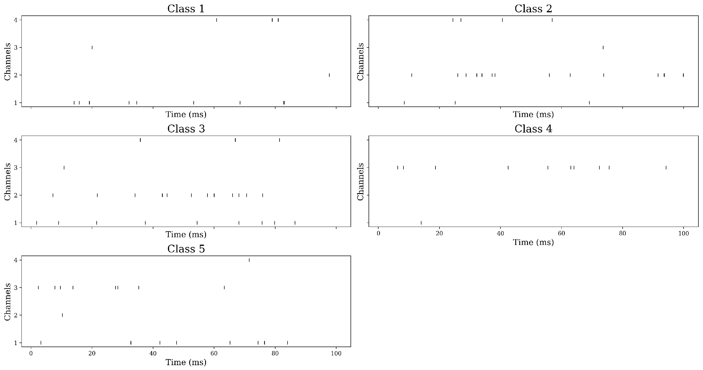
Two synthetic multi-class classification problems are tested to assess the proposal’s performance. These tasks, described in Norton & Ventura [31], are called Frequency Recognition (FR) and Pattern Recognition (PR). The FR problem consists of four inputs and five classes (referred to as FR5), where each input can have a fire rate of either slow or high, depending on the class.

Table 1. Frequency states of channels for the five classes in the FR5 task. “H” and “L” are high (100 Hz) and low frequency (10 Hz), respectively.

	Channel 1	Channel 2	Channel 3	Channel 4
Class 1	H	L	L	L
Class 2	L	H	L	L
Class 3	H	H	L	L
Class 4	L	L	H	L
Class 5	H	L	H	L

shows the channel’s frequency state distribution for all classes. The high frequency was set at 100 Hz, and the low frequency at 10 Hz. For each class, 1000 samples of 100 ms were created using a template and then jittered (In this context, jittering refers to a small variation.) in frequency. An example of each class is presented in Figure 3. Part of the challenge in this task is to detect a variety of frequencies while ignoring a channel (Channel 4) that never exhibits a high frequency.

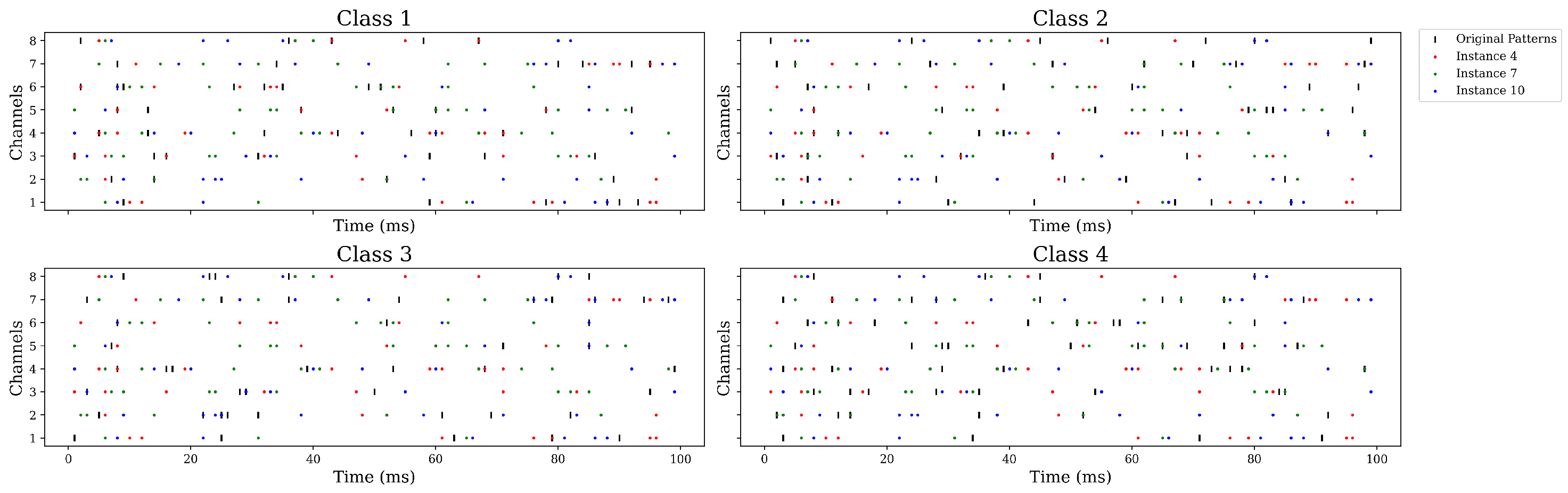
The PR problem has eight input channels and a different number of classes. To name them, PR4, PR8, and PR12 will be referred to as the fourth, eighth, and twelfth class problems, respectively. A random spike pattern is generated for each input channel, and instances are created by applying perturbations to these patterns. Similar to FR5, 1000 instances per class were created. Figure 4 shows an example of three instances per class of the PR4 task. These problems are, compared with FR5, more complex since each spike is individually jittered.

These classification tasks challenge the model from different fronts: the FR dataset challenges the model with a variety of combinations of frequencies as well as the task of ignoring one channel since channel 4 always presents a low frequency [31]; the PR datasets increase the complexity by incrementing the number of input channels and classes, specifically in PR8 and P12.

Furthermore, tests on two real-world datasets are also included. The MNIST dataset is a benchmark commonly used in machine learning for image classification and pattern recognition tasks. It consists of 70,000 grayscale images of handwritten digits (0–9). The dataset images have 28 × 28 pixels. The Neuromorphic MNIST (N-MNIST) dataset, introduced by Orchard et al. [44], records the standard MNIST dataset using a neuromorphic vision sensor Asynchronous Time-based Image Sensor (ATIS).

The FSDD [45] is an open audio dataset designed for benchmarking speech recognition systems. It consists of spoken digits (0–9) pronounced by multiple speakers in English. Each sample is a single-channel waveform recorded at 8 kHz. The dataset consists of 2000 audio recordings.

The preparation of the FSDD involved two main steps. First, the Mel-Frequency Cepstral Coefficients (MFCCs) were extracted from the samples to capture relevant spectral features. Then, the extracted features were converted into spike trains using a Poisson rate coding scheme, where the firing rate was proportional to the signal intensity. This procedure was adopted from the method of Tian et al. [38]. In contrast, the N-MNIST dataset required minimal preprocessing: the original 28 × 28 event-based frames were downsampled to 17 × 17, reducing the number of input channels to 289.

2.2. LSM

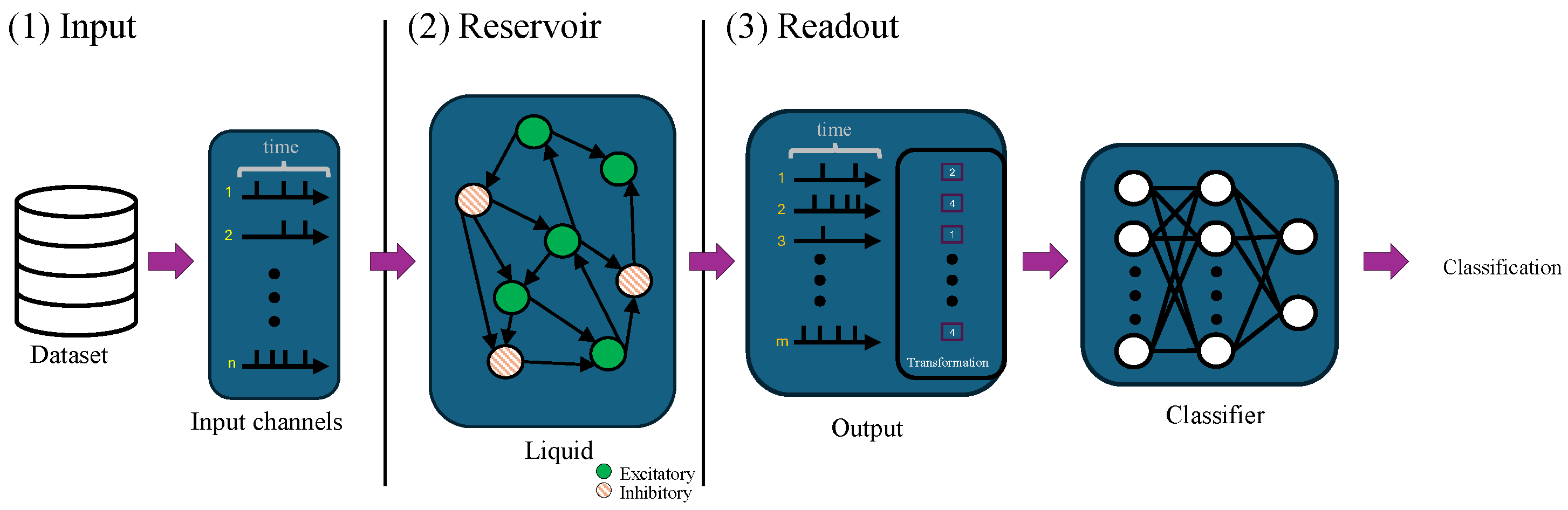
The LSM is a framework that specializes in solving spatiotemporal tasks and is based on RC. Therefore, there are two distinct parts of an LSM: the reservoir and the readout. The reservoir, also known as liquid, serves as a kernel of spiking neurons that project input data into liquid states, which are high-dimensional representations of the internal states of the liquid. On the other hand, the readout serves as a memory-less function for interpreting liquid states, specifically trained for a given task. The pipeline of an LSM, shown in Figure 5, is as follows:

• Input: A dataset provides multichannel temporal inputs, each corresponding to a distinct signal. If the dataset consists of continuous signals, then the data must be encoded as spike trains. Then, the channels project the stream data into randomly selected neurons in the liquid.
  In this work, a 50% Input-to-Liquid connectivity ($Con{n}_{I-L}$) is used, meaning that each channel connects to half the number of randomly selected neurons in the liquid. The corresponding input synaptic weights are sampled from a uniform distribution $U(1,50)$.
• Reservoir: The liquid represents the core mechanism in an LSM. It consists of an R-SNN, which includes both excitatory and inhibitory neurons. Following the classical LSM formulation introduced by Maass et al. [2], neurons are organized into excitatory and inhibitory populations, where excitatory neurons produce positive (excitatory) postsynaptic connections and inhibitory neurons produce negative (inhibitory) ones.
  In this work, the LIF neuronal units are randomly placed in a 2D space, and their connections and synaptic values are determined by the distance between neurons. As spikes propagate through this connected network, the liquid transforms inputs into dynamic, high-dimensional internal states, referred to as liquid states. For state extraction, spike responses from excitatory neurons are recorded across the full simulation window and used to construct the liquid state representation, as excitatory neurons provide a more stable and informative representation of the liquid dynamics, while inhibitory neurons primarily regulate internal activity. These state vectors are then provided to the readout stage for classification.
  All liquid simulations were conducted using the NEST simulator package [15], employing the standard configuration of the LIF neuron model “iaf_psc_alpha”.
• Readout: After the liquid’s response, the states are sampled and transformed into a static representation known as a state vector. This process is necessary every time the readout block is memory-less. The most common transformation techniques include the spike count (the total number of spikes) and spike rate (the total number of spikes divided by the signal’s length). Each state representation is then passed to a classifier, which is trained to perform a specific task.

Our approach employs the spike rate transformation, which favors the relative activity intensity [46]. Moreover, the readout function is implemented as a one-vs-rest linear classifier composed of n independent Perceptrons, each trained to recognize one class against the rest using Stochastic Gradient Descent (SGD). The classification is fitted against all the other classes, assigning the class of the Perceptron with the greatest confidence. As parameters, the SGD uses a maximum iteration ($Ma{x}_I$) of 1000, a tolerance ($Tol$) of $1\times {10}^{-3}$, and a L2 regularization process with $\alpha$ of $1\times {10}^{-4}$. This readout function was selected for its simplicity, which adds value to the liquid process.

A summary of the parameters used in this pipeline is shown in

Table 2. Parameters used in the LSM model.

Component	Parameter	Value
Input-to-Liquid connections	Input connectivity	50%
	Input synaptic weights	$U(1,50)$
	Excitatory neurons	80%
Liquid (Reservoir)	Neuron model	LIF
Neuron parameters (LIF)	Initial potential ($V_m$)	−70 mV
	Resting potential ($E_L$)	−70 mV
	Capacity of membrane ($C_m$)	100 pF
	Reset potential ($V_{reset}$)	−70 mV
	Input Noise ($I_{noise}$)	100 pA
Readout	State Window	100%
	Encoding method	Spike-rate
	Classifier	One-vs-rest Perceptron
	Maximum Iteration	1000
	Tolerance	$1\times {10}^{-3}$
	Regularization factor ($\alpha$)	$1\times {10}^{-4}$

.

2.3. GA

This section outlines the proposed GA adopted in this study. The GA serves as the optimization strategy for configuring the liquid’s structure, guiding the search toward architectures that enhance the LSM’s classification performance. The general framework followed is shown in Figure 2. The encoding scheme, genetic operators, selection mechanism, and fitness evaluation process are described in detail below.

2.3.1. Encoding, Initialization & Population

A suitable representation of neural architectures is essential for effective evolutionary optimization in NE. The objective is for the representation encoding, often referred to as genotype, to contain the necessary components and information of the models to define a proper search space. In that sense, the proposed encoding considers two sections: neuron configurations and positions. Regarding the former, four parameters are considered:

• Voltage threshold $V_{th}$: A lower threshold makes the neuron more sensitive to incoming pulses, allowing it to fire with less input frequency.
• Membrane time constant ${\tau }_m$: This parameter defines how quickly the membrane potential returns to rest after perturbation. A higher value extends the summation window, allowing distant spikes to contribute more significantly.
• Refractory period $\mathrm{\Delta }{t}_{\mathrm{ref}}$: The time during which a neuron cannot fire after spiking. A lower value allows faster recovery.
• Polarity: Defines whether a neuron is excitatory or inhibitory. Excitatory neurons increase the membrane potential of postsynaptic neurons, while inhibitory neurons decrease it. This property might be represented as the sign of the neuron’s outgoing connections.

On the other hand, the X and Y coordinates in a 2D space (liquid) formed the positional information of the neuronal units, which also establish the connectivity of the liquid.

Three restrictions are necessary to establish correct encoding:

• Parameters ${\tau }_m$, $\mathrm{\Delta }{t}_{\mathrm{ref}}$, X and Y can not be equal or lower than 0. Violations are mapped to a small default value of $0.01$.
• Voltage threshold $V_{th}$ must exceed reset potential $V_{\mathrm{reset}}$. If this condition is not met, $V_{\mathrm{reset}}$ is lowered $5$ mV below $V_{th}$.
• Neurons must have unique positions. If any overlap occurs, one conflicting neuron is reassigned to a random valid position.

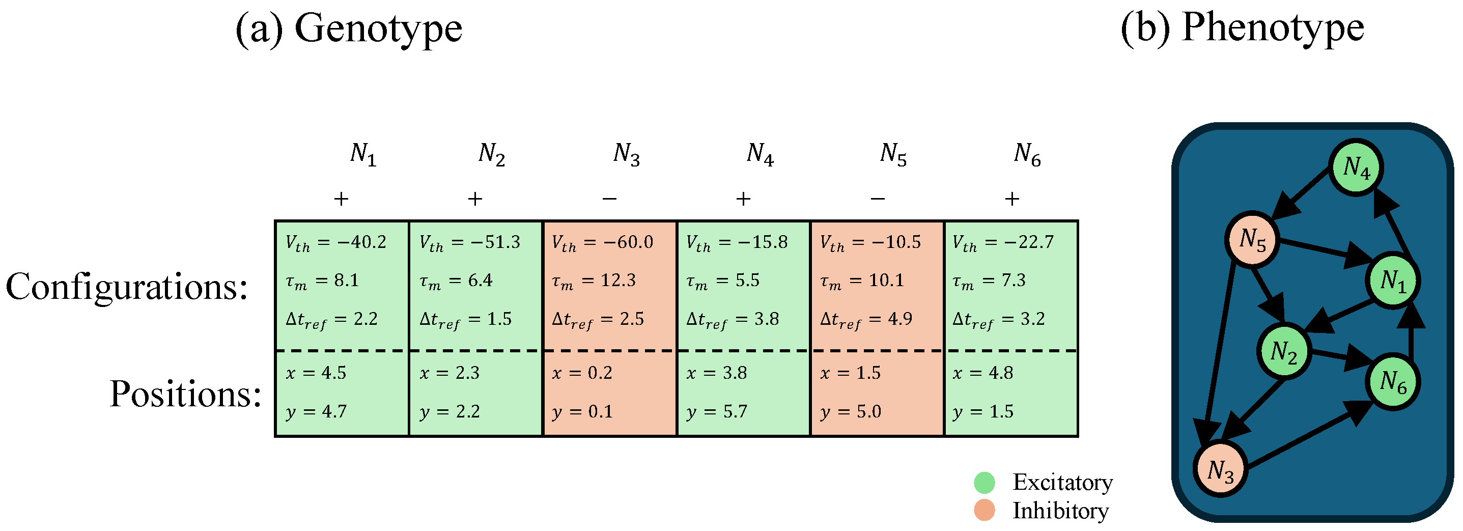
Each individual in the population, also referred to as a chromosome, is composed of n genes, where n is the number of neurons in the liquid. Each gene encodes the attributes of a single neuron, combining both its configuration parameters and its spatial position within the liquid. As a result, the dimensionality of the genotype grows linearly with the number of neurons. Figure 6 shows an encoding and decoding example. Specifically, Figure 6a shows an example of a valid genotype of 6 neurons.

Moreover, the neuron’s position defines the connectivity of the liquid using a pairwise test to connect each possible pair of source ($N_s$) and target ($N_t$) neurons, with a probability of p. The p is calculated as the Probability Density Function (PDF) of a Gaussian Distribution of the distance (D) between $N_s$ and $N_t$. Equation (1) illustrates the estimation of the probability $p_{st}$ of the neuron $N_s$ being connected to neuron $N_t$; with this procedure, the closer the neurons are to each other, the greater the chance they are connected. This follows biological accuracy [47,48] known as Peter’s rule. This distance-based rule is depicted in Equation (2); a shorter connection will have a more substantial impact on postsynaptic neurons, which emulates the biological principle that shorter connections tend to have more substantial synaptic weights due to reduced delays and energy costs [48].

$$p_{st}={\displaystyle \frac{1}{\sqrt{2\pi }}}{e}^{-{\displaystyle \frac{D{(N_s,N_t)}^2}{4}}}$$

(1)

$$S{W}_{st}=SS\times p_{st}$$

(2)

where $D(·)$ represents the Euclidean distance between neurons $N_s$ and $N_t$, $p_{st}$ is the Gaussian probability associated with that distance, and $SS$ denotes the synaptic strength scaling factor. Since the Gaussian probability density function is bounded, the resulting synaptic weights are also bounded. Given the synaptic strength parameter ($SS=200$), the maximum weight value occurs when the distance between two neurons is close to zero, resulting in a value close to $\pm 80$. Larger distances produce weights close to zero.

The population consists of 50 individuals, and this size remains fixed throughout the evolutionary process. At initialization, each individual’s parameters are randomly defined. To manage computational cost, the liquid size was set to 20 LIF neurons for the synthetic datasets and increased to 300 LIF neurons for the N-MNIST and FSDD datasets. The polarity initialization was adapted to have 80% excitatory neurons, aligning with biological ratios observed in cortical regions [49]; every neuron has an 80% probability of being excitatory.

Parameters $V_{th}$, ${\tau }_m$, $\mathrm{\Delta }{t}_{\mathrm{ref}}$, X, and Y are randomly selected uniformly from specific ranges, shown in

Table 3. Parameter ranges. It shows the normal values found in the literature and the ranges used for random selection for each parameter. “-” means that the value does not apply.

Parameter	Normal Value	Range
$V_{th}$	$-55$ mV	$[-69,-10]$
${\tau }_m$	10 ms	$[6,14]$
$\mathrm{\Delta }{t}_{\mathrm{ref}}$	2 ms	$[0.5,4]$
Polarity	80%	-
X and Y	-	$[0,6]$/$[0,15]$

. The ranges of $V_{th}$, ${\tau }_m$, $\mathrm{\Delta }{t}_{\mathrm{ref}}$ were selected to have the mean value closer to the normal value. On the other hand, the ranges of X and Y were established following preliminary experiments, in which different upper limits were tested. It was observed that larger values decreased the spiking activity, whereas smaller values saturated the liquid activity. For this reason, both X and Y were constrained to an upper limit of 6, corresponding to a $6\times 6$ spatial grid, which provided a balanced spatial scale and maintained computational manageability for the synthetic datasets. For the larger-scale experiments, the spatial domain was expanded to a $15\times 15$ grid to preserve an appropriate neuron distribution and connectivity structure. Nevertheless, it is crucial to validate these ranges with further experimentation.

2.3.2. Evaluation

The process of evaluating an individual starts by decoding the genotype into a corresponding phenotype (Figure 6b). This task involves setting the individual neuron parameters, such as their configuration and positions, as well as defining which neurons will receive an input connection. Once the network is instantiated, the individual is simulated: input patterns are presented to the liquid, and the resulting spike responses are recorded as liquid states. These states are then transformed into a static state vector, which is fed into the readout block for classification. The individual’s performance is measured using classification accuracy as the objective function.

2.3.3. Parent Selection

A tournament selection mechanism was chosen for its simplicity and robustness. Tournament selection is a parent selection strategy commonly used in EAs. In this method, a predefined number of individuals, referred to as the tournament size, are randomly sampled from the population. These individuals compete based on their fitness values, and the one with the highest fitness is selected as a parent. This process is repeated as needed to generate the required number of parents.

2.3.4. Crossover

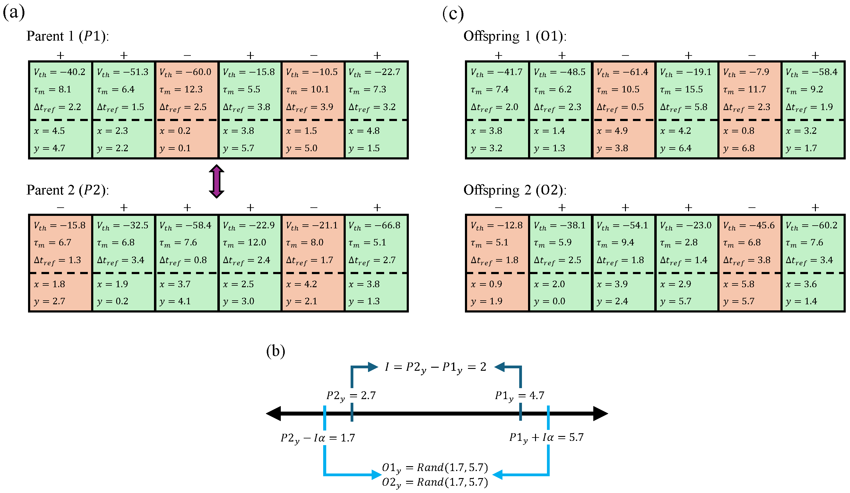
The crossover variant operation promotes the exploitation of the parents’ characteristics. The Blend Crossover with $\alpha =0.5$, referred to as BLX-$\alpha$, was selected in this work. This operator is designed for real-valued encoding and creates offspring by sampling each gene from a uniform distribution defined by the parent genes and a blending parameter $\alpha$. Figure 7 illustrates the crossover mechanism.

First, the parents’ genotypes are aligned (Figure 7a). Specifically, for each gene, the offspring value is drawn from the interval $[x_{min}-I\alpha ,x_{max}+I\alpha ]$, where $x_{min}$ and $x_{max}$ are the values of the corresponding gene from the two parents, and $I=x_{max}-x_{min}$ defines the difference between the two values. This approach promotes exploration beyond the parental range while maintaining genetic continuity. Figure 7b shows an example of the calculation. Finally, this process is repeated for every parameter in every gene, resulting in two offspring (Figure 7c). Polarity, being a binary parameter (excitatory or inhibitory), does not undergo this crossover process and is inherited directly from the parents.

2.3.5. Mutation

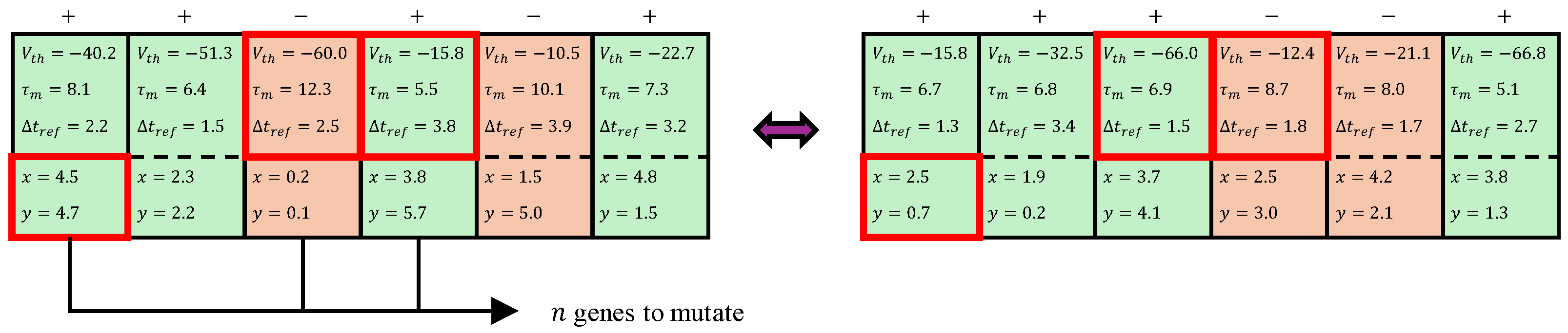
Unlike crossover, which seeks to promote exploitation, the mutation operator is responsible for providing exploration. In this work, a random subset of n neurons, where n stands for half the total number of neurons in the liquid, is re-initialized and derived from the original ranges. Furthermore, only the configurations or the positions are affected based on a 50% probability. Figure 8 depicts an example of this process, where the configurations of genes 3 and 4, and the position of gene 1 are re-initialized. Although these mutations are relatively strong, they were intentionally chosen to promote exploration, where small perturbations may not always yield meaningful behavioral differences in the network.

2.3.6. Replacement & Stop Criteria

A generational replacement is adopted, including an elitism process to preserve a percentage of the best-suited individuals in every generation. Furthermore, if the maximum number of generations is reached or any individual achieves 100% accuracy, the evolutionary process terminates.

2.4. Methodology & Calibration

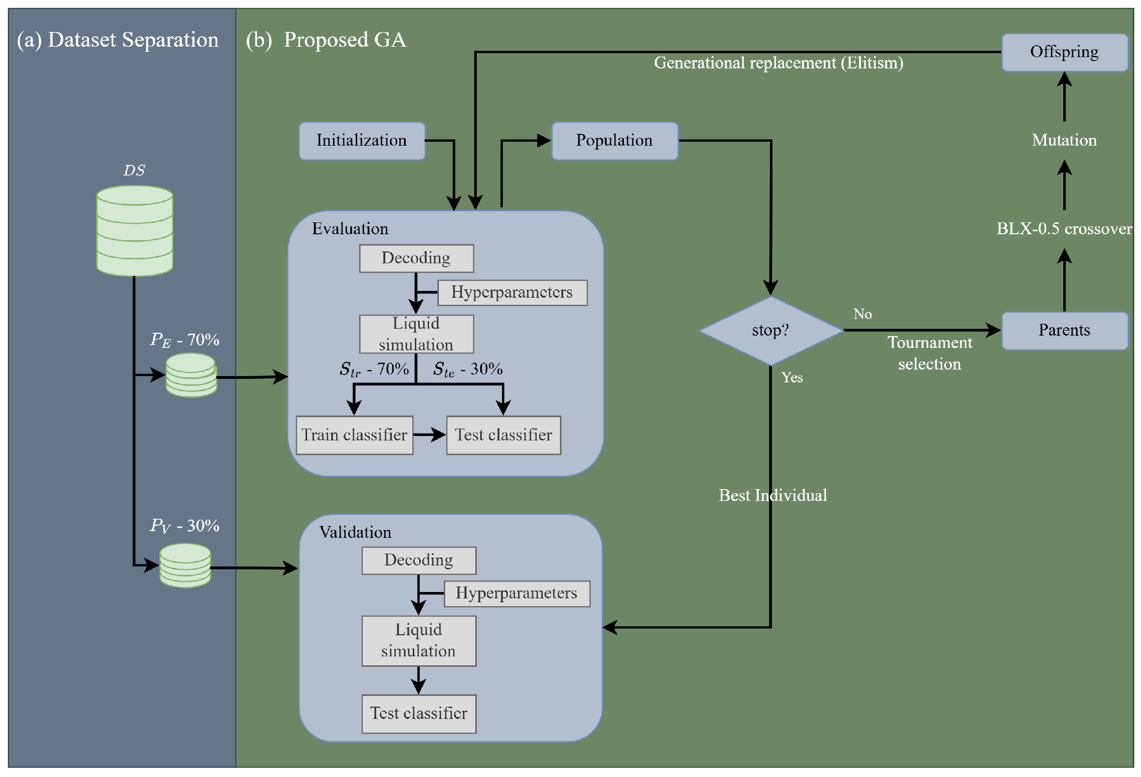
Figure 9 illustrates the complete pipeline of the proposed methodology, integrating the data partitioning and the evolutionary optimization process described above. The first phase (Figure 9a) divides the dataset into two partitions: an Evolutionary partition $P_E$ (70%), intended for the GA process, and a Validation partition $P_V$ (30%), used on the best individual obtained after the GA process. The second phase entails the GA-proposed process (Figure 9b). For each individual, the evolutionary partition $P_E$ is internally partitioned into training and testing subsets to train and evaluate the readout model, ensuring a fair estimate of classification performance.

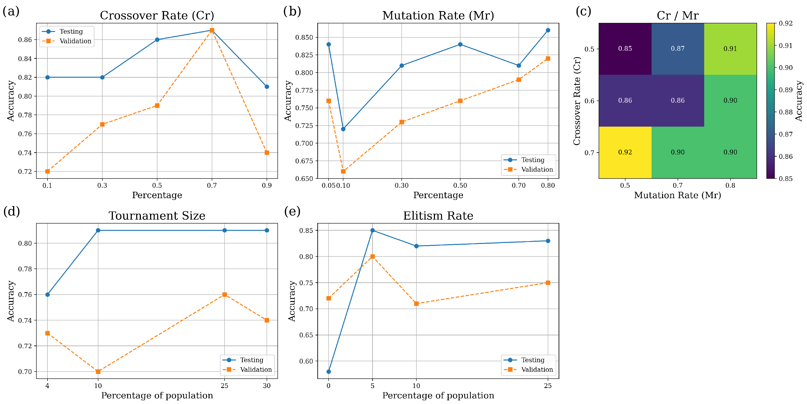
A calibration process was used to establish the values for the crossover rate (Cr), mutation rate (Mr), Tournament size, and Elitism. To perform this, ten executions of the GA with a reduced number of instances of the FR5 were conducted with different values. While a full grid search across all parameter combinations could yield more optimal configurations, such an approach was not implemented due to the high computational cost associated with simulating each combination. Figure 10 shows the mean accuracy obtained in experiments. For Cr, it was observed that 70% performed well on both the Testing and Validation, followed by 50%. Interestingly, 90% exhibit a significant drop in performance (Figure 10a). The Mr parameter showed an increasing performance as the percentage increment increased. Two interesting peaks appeared on 50% and 80% (Figure 10b). Following these observations, five additional experiments were performed for every combination of 50%, 60%, 70% for Cr and 50%, 70%, and 80% for Mr (Figure 10c). Interestingly, the best results reside within the high Cr or Mr percentages. Nevertheless, having both parameters in a high percentage increased the number of evaluated individuals, augmenting the computational cost. Therefore, a 70% Cr and 50% was selected. Notably, higher mutation rates yielded competitive results, indicating the potential suitability of alternative approaches, such as Evolutionary Strategies (ES). Regarding tournament size and elitism, the analysis shows better results at 25%, which forms a tournament of 12 individuals, and 5%, which sets three individuals for elitism, respectively.

Table 4. Parameter summary. The values in bold were calibrated during a number of experiments, whereas the rest were selected based on prior experience.

Parameter	Value
Population size	50
Generations	100
Cr	70%
Mr	50%
Tournament size	25% (12 individuals)
Elitism	5% (3 individuals)

summarizes the parameter calibrations.

To test the implementation, 30 executions were performed on the FR5, PR4, PR8, and PR12 tasks. In contrast, due to computational limitations, only five executions were carried out for the N-MNIST dataset and the FSDD. The DEAP [51] library was used for GA implementation, programmed in Python 3.10. Experiments were conducted on a high-performance machine equipped with two Intel® Xeon® Gold CPUs (Model 6226R) with 72 logical processors, enabling parallel evaluation of individuals. Given a population size of 50 individuals and 100 generations, each evolutionary run required approximately 5000 fitness evaluations. In practice, runs on the synthetic benchmark datasets required approximately 6 h per execution. For real-world datasets involving larger liquids and higher input dimensionality, the runtime increased to approximately 24–30 h per run. These runtimes are comparable to or shorter than those reported in related work, such as Tian et al. [38], who reported approximately 16.3 days for N-MNIST and 3.3 days for FSDD, and Zhou et al. [39], who reported runtimes of around 42 h.

3. Results

3.1. Experiments on Synthetic Datasets

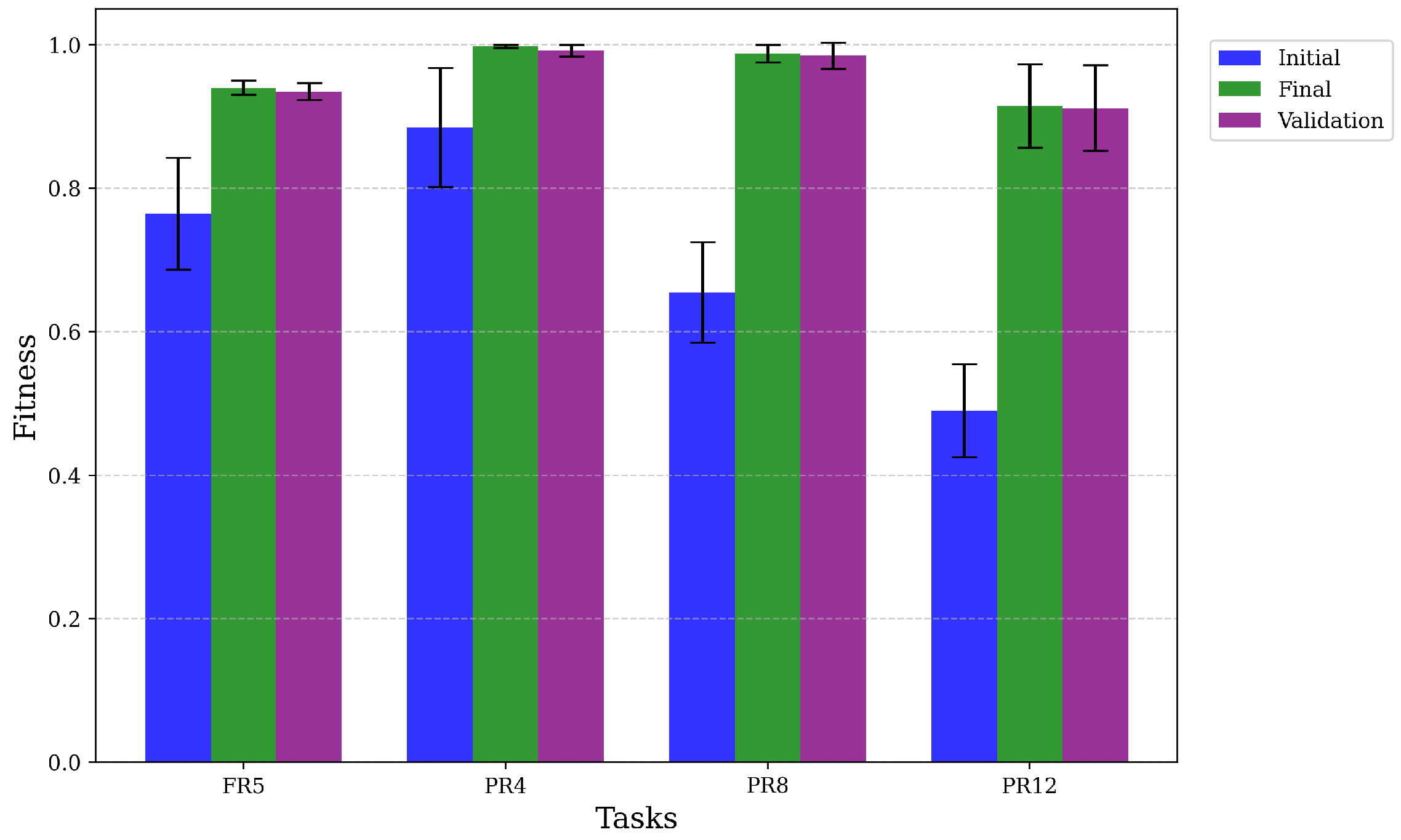
To establish a baseline contrast, Figure 11 presents a comparison among the best initial fitness, the best final fitness, and the validation process. This shows a robust generalization, as evidenced by reduced overfitting and improved validation accuracy.

Table 5. Performance comparison among Norton & Ventura [31] (SDSM), Alvarez-Canchila et al. [41] (PSO), and this work. The $x_B$, $\overline{x}$, $x_M$, $x_W$, and $\sigma$ represent the best value, mean, median, worst value, and standard deviation, respectively. The “-” mark stands for data not available. All values in bold signify the best values.

Task	Statistical	SDSM	PSO	GA (This)
FR5	$x_B$	0.944	0.9080	0.9610
	$\overline{x}$	0.7822	0.8158	0.9384
	$x_M$	-	0.8700	0.9387
	$x_W$	-	0.5440	0.9187
	$\sigma$	-	0.0973	0.0102
PR4	$x_B$	0.99	1.0000	1.0000
	$\overline{x}$	0.9197	0.9828	0.9971
	$x_M$	-	1.0000	0.9983
	$x_W$	-	0.6925	0.9725
	$\sigma$	-	0.0645	0.0053
PR8	$x_B$	0.98	0.9662	1.0000
	$\overline{x}$	0.759	0.8910	0.9880
	$x_M$	-	0.9663	0.9950
	$x_W$	-	0.4775	0.9400
	$\sigma$	-	0.1483	0.0149
PR12	$x_B$	0.9167	0.9975	0.9975
	$\overline{x}$	0.7562	0.9373	0.9162
	$x_M$	-	0.9750	0.9257
	$x_W$	-	0.2742	0.7447
	$\sigma$	-	0.1379	0.0597

shows a comparison of results among this approach and the Norton & Ventura [31] approach, referenced as SDSM, and Alvarez-Canchila et al. [41], referenced as PSO. The results reported for the SDSM [29] method were taken from the original publication. For the PSO method [41], the authors of that work provided their full experimental results, which allowed us to perform statistical comparisons between both approaches.

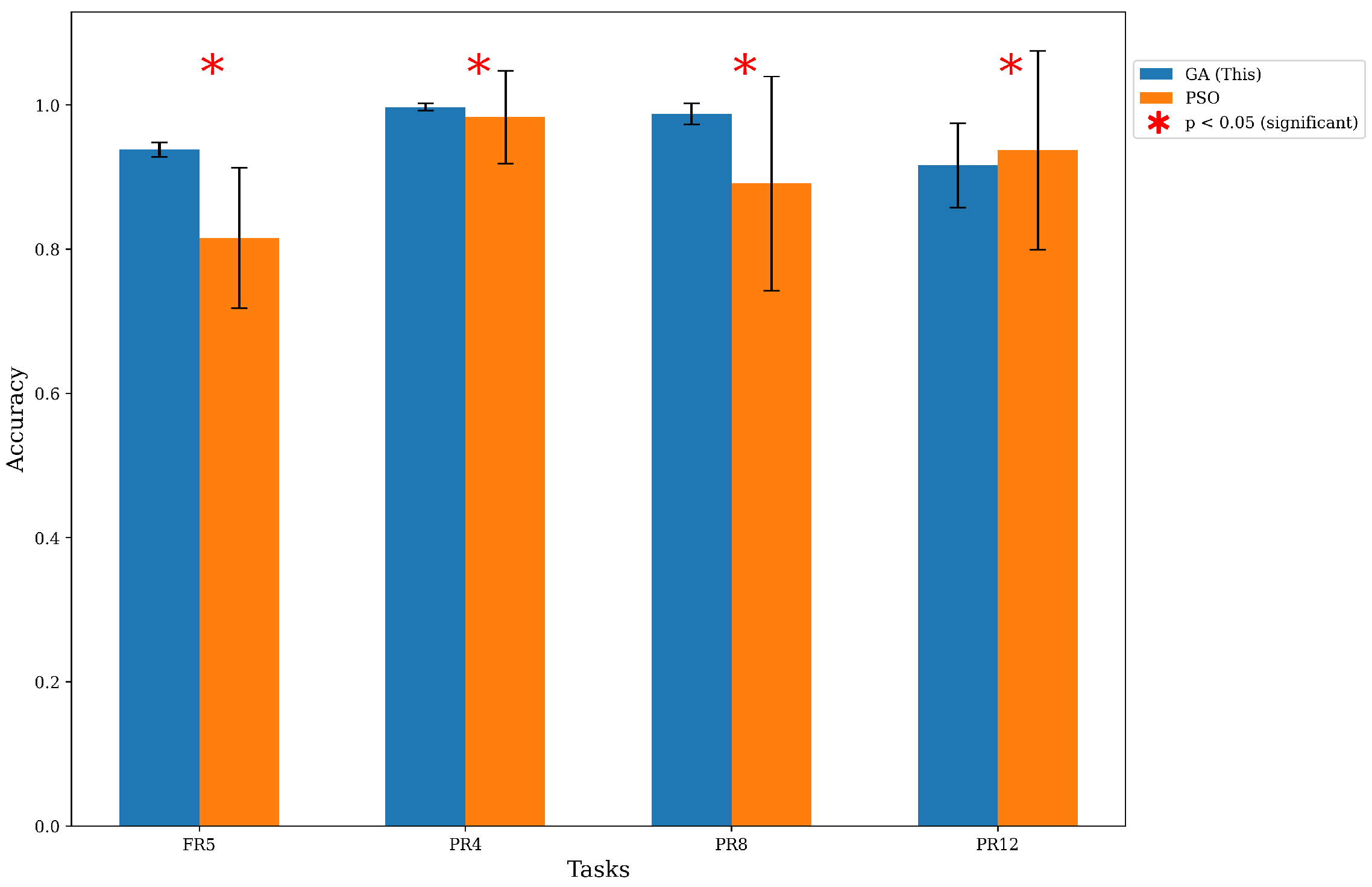
The proposed method outperformed all metrics in all tasks except the mean and median values of FR12. To assess statistical significance, the Shapiro–Wilk test was first applied to evaluate the normality of the accuracy distributions. Since the normality assumption was not met, the non-parametric Kruskal–Wallis test was used to compare the performance of the GA method and PSO. The results are summarized in Figure 12; significant differences are observed across all tasks. In FR5, PR4, and PR8, these differences favor our approach. Nevertheless, the case of PR12 warrants further analysis, as statistical metrics may indicate equal capabilities between our approach and PSO, yet significant differences were observed.

Even though PSO achieved better mean and median values, our GA method tied their best results and outperformed their worst cases, as well as the standard deviation. This indicated that PSO had higher top-end performance, with some extreme values contributing to the standard deviation.

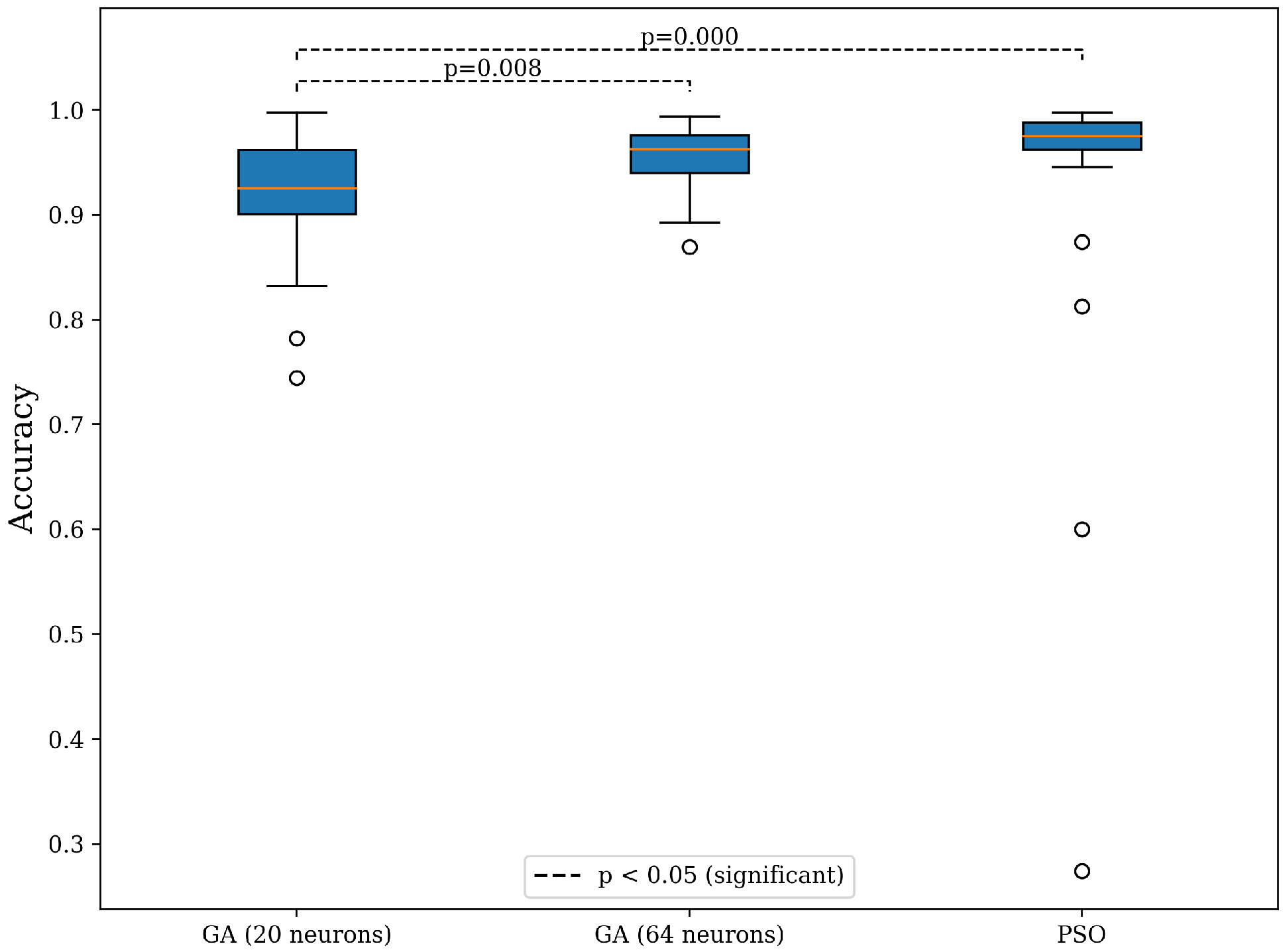
To further assess this, 30 additional experiments were performed, increasing the number of neurons to 64, matching the model of Alvarez-Canchila et al. [41].

Table 6. Performance comparison among Alvarez-Canchila et al. [41] (PSO), and this work with 20 and 64 neurons. The $x_B$, $\overline{x}$, $x_M$, $x_W$, and $\sigma$ represent the best value, mean, median, worst value, and standard deviation, respectively. All values in bold signify the best values.

Task	Statistical	PSO	GA (20 Neurons)	GA (64 Neurons)
PR12	$x_B$	0.9975	0.9975	0.9939
	$\overline{x}$	0.9373	0.9162	0.9546
	$x_M$	0.9750	0.9257	0.9628
	$x_W$	0.2742	0.7447	0.8694
	$\sigma$	0.1379	0.0597	0.0298

presents a comparison of statistical metrics, demonstrating an improvement in our method. Given the non-normal distribution detected by the Shapiro–Wilk test, a Kruskal–Wallis test followed by Dunn’s post hoc test (p < 0.05) was applied among the PSO, GA with 20 neurons, and GA with 64 neurons. As shown in Figure 13, no statistically significant differences were observed between the proposed method and PSO. Nevertheless, PSO yields a wider spread of results, including more extreme low-performing outliers, whereas the proposed method maintains more consistent performance.

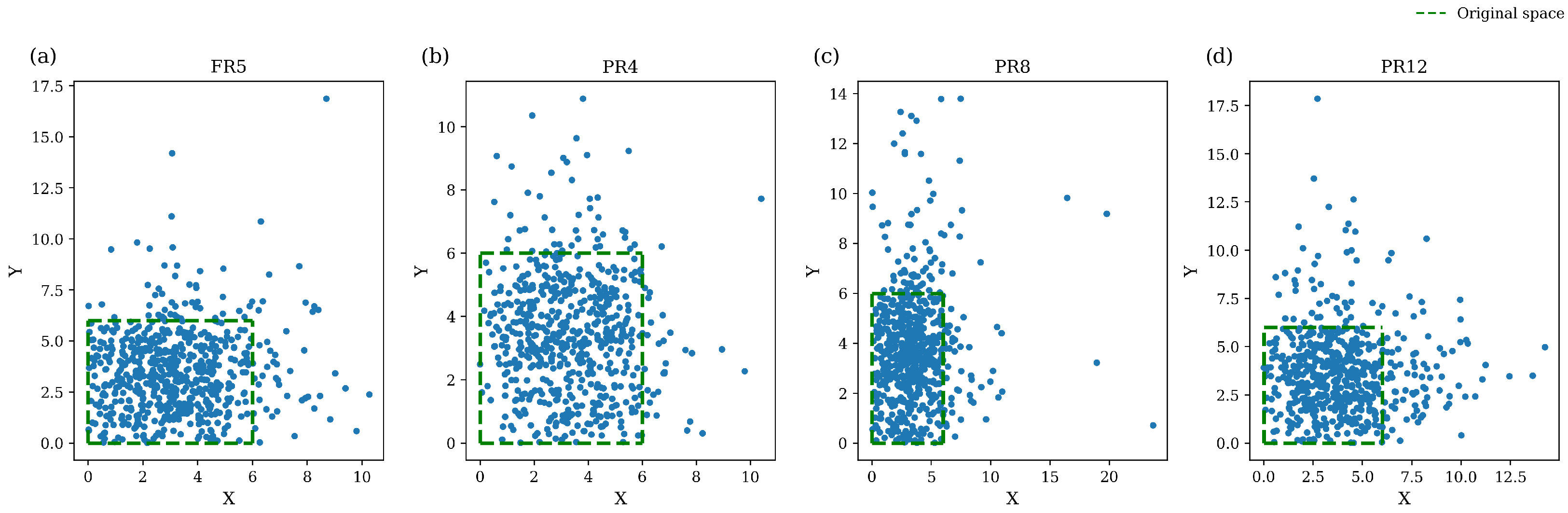
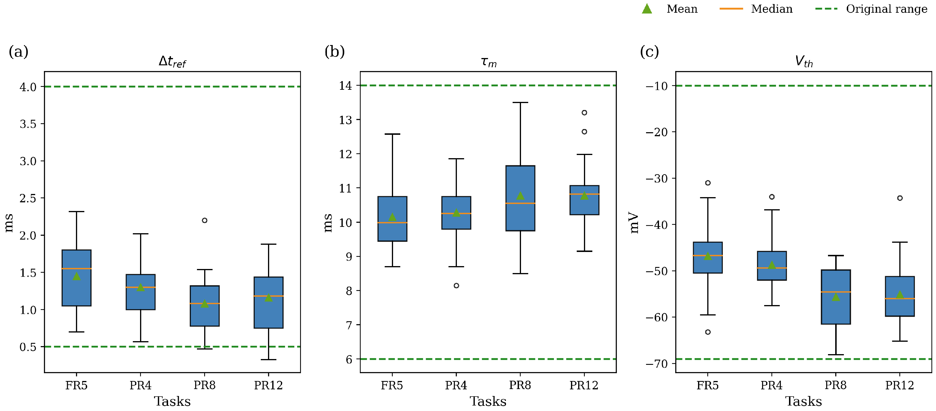
Evaluating the final neuronal configuration, namely $V_{th}$, ${\tau }_m$, and $\mathrm{\Delta }{t}_{\mathrm{ref}}$, and the position distribution of the best individuals from the four tasks with our GA method (excluding the GA with 64 neurons since it was only tested on PR12), Figure 14 and Figure 15 show that most values remain within the original initialization ranges. The neuron configurations tend to converge within narrower intervals, although the resulting distributions differ from task to task. Therefore, these statistics should be interpreted separately for each benchmark rather than as a global trend across all tasks. In contrast, the neuron position distributions do not exhibit a clearly discernible pattern.

3.2. Experiments on Real-World Benchmarks

In addition to the synthetic datasets, the proposed method was evaluated on two standard benchmarks: N-MNIST and FSDD. These datasets present more complex spatiotemporal patterns, offering a stronger test of the model’s capabilities. To account for the increased complexity, the liquid size was increased to 300 neurons, the initial positional grid was set to 15 × 15, and only five executions were performed per task. The results reported for Tian et al. [38] and Zhou et al. [39] were taken from their respective publications and are used here as reference.

Table 7. Comparison of performance on N-MNIST and FSDD datasets. The “-” mark stands for data not available.

Method	N-MNIST		FSDD
	Neurons	Accuracy	Neurons	Accuracy
Tian et al. [38]	1000	92.50%	1000	84.50%
Zhou et al. [39]	-	92.80%	-	-
Ours	300	90.65% (±1.59%)	300	81.47% (±2.12%)

shows that while our method did not achieve the highest accuracy, it reached competitive results using significantly fewer neurons. For instance, Tian et al. [38] employ reservoirs with 1000 neurons, whereas our approach achieves comparable performance using only 300 neurons. Zhou et al. [39] propose an architecture search method that adjusts structural aspects of the reservoir, including the number of neurons during optimization; however, the exact number of neurons in their final architectures is not explicitly reported. Nevertheless, our results indicate that competitive performance can be obtained with a more compact architecture. Since the computational cost of simulating SNNs scales with the number of neurons and synaptic interactions, reducing the network size reduces computational complexity and improves efficiency, making the model suitable for resource-constrained environments, such as neuromorphic hardware platforms, embedded systems, and edge computing devices.

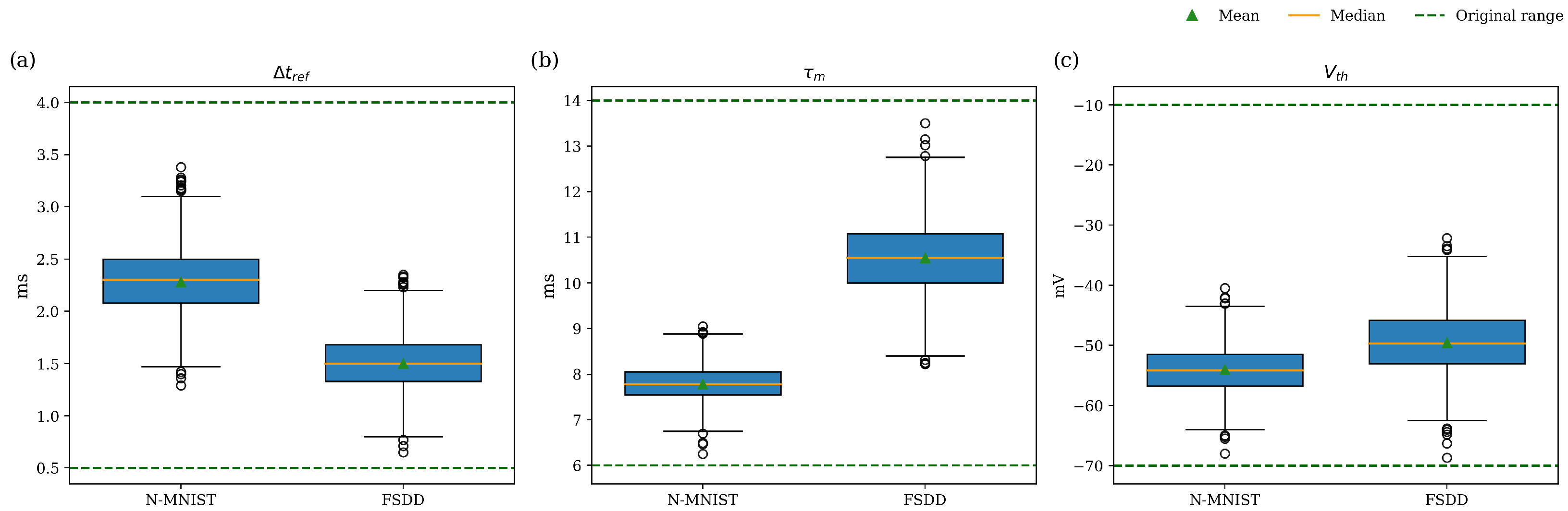
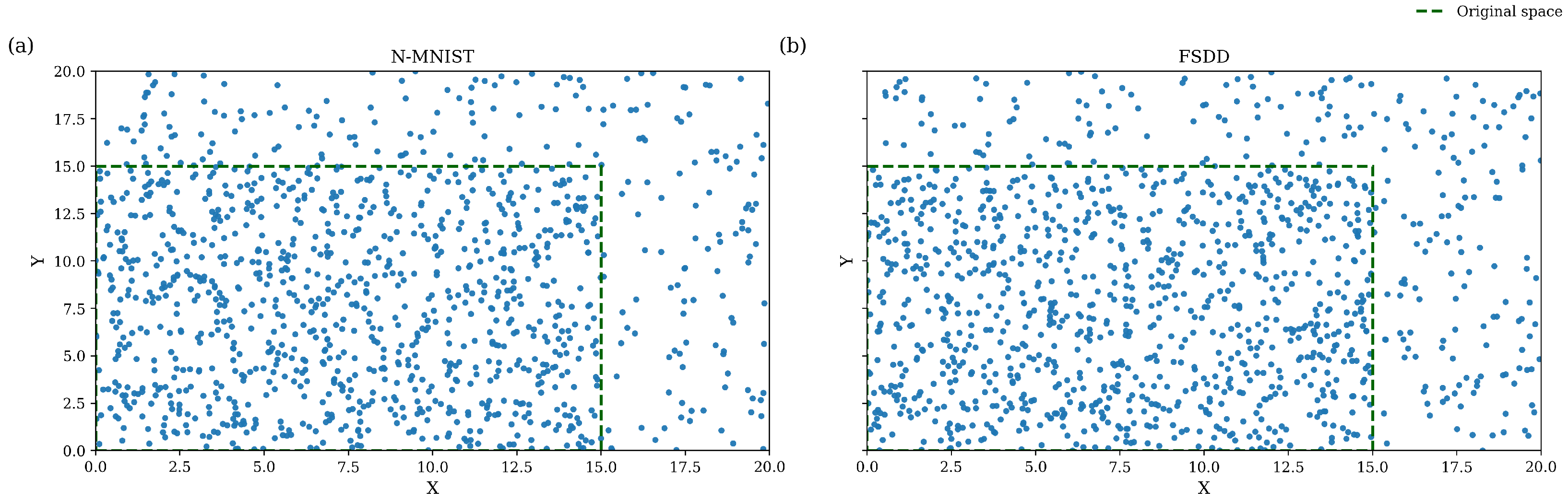
Similarly to before, Figure 16 and Figure 17 show the final neuronal configuration and position distribution of the best individuals from these tasks, respectively. The observations obtained from the synthetic experiments remain consistent: neuron configurations converge to narrower ranges depending on the task, while neuron positions remain dispersed without exhibiting a clear spatial pattern.

4. Discussion & Conclusions

The LSM model, an RC approach that combines R-SNN with simple linear classification methods, excels in several spatiotemporal applications. Among their qualities, LSMs harness the complexity of neuron models, such as the LIF model, to learn spatiotemporal features and patterns in complex time series. Although the traditional LSM formulation assumes a fixed, untrained liquid (reservoir), recent research has relaxed this constraint by introducing training or optimization strategies for the R-SNN, thereby enhancing the liquid capabilities. Moreover, most state-of-the-art (SOTA) methods do not exploit the neuron parameters available, such as the refractory period ($\mathrm{\Delta }{t}_{ref}$), the membrane time constant (${\tau }_m$), and the spike threshold ($V_{th}$), to optimize the performance of the liquid and reside entirely on the synaptic connections.

In this work, a novel NE approach for optimizing LSM based on a GA encoding neuron configurations and position was presented. To validate the method, two different approaches were used. First, four synthetic classification tasks, namely a Frequency Recognition task with five classes (FR5) and three Pattern Recognition tasks with 4 (PR4), 8 (PR8), and 12 (PR12) classes. Results were compared with two similar approaches: the SDSM learning technique introduced by Norton & Ventura [31] and a PSO metaheuristic method proposed by Alvarez-Canchila et al. [41]. Second, two classical datasets were utilized, N-MNIST and FSDD, and the results were compared against SOTA methods proposed by Tian et al. [38] and Zhou et al. [39]. To manage computational cost, the size of the liquid was limited to 20 LIF neurons for the synthetic datasets and 300 LIF neurons for the N-MNIST and the FSDD.

The method achieved SOTA results in the synthetic tasks, with mean accuracies of $93.84\%$ in FR5, $99.74\%$ in PR4, $98.80\%$ in PR8, and $91.62\%$ in PR12. Furthermore, our approach yielded better results across all statistical metrics investigated, with significant differences proven by the Kruskal–Wallis test, except for PR12. Further examination of the PR12 case revealed that the PSO method achieved higher top-end performance while exhibiting several suboptimal runs (e.g., the worst value of $27.42\%$ compared to $74.47\%$ for our GA approach). The number of neurons was increased to match the 64 neurons from the PSO proposal, resulting in a mean accuracy of $95.46\%$ in PR12 with no significant difference.

Our results suggest that, while PSO was capable of reaching competitive results, our NE GA-based approach yielded more stable performance across runs, showing a more robust and generalizable approach. Incorporating neuron configurations into the optimization process proved to be an efficient strategy, as it enabled the exploration of diverse and dynamic regimes within the liquid, leading to improved task-specific performance without increasing the network size.

The method achieved SOTA results in the synthetic tasks, with mean accuracies of $93.84\%$ in FR5, $99.74\%$ in PR4, $98.80\%$ in PR8, and $91.62\%$ in PR12. Furthermore, our approach yielded better results across all statistical metrics investigated, with significant differences confirmed by the Kruskal–Wallis test, except for PR12. Further analysis of this case revealed that, although the PSO method exhibited greater variability across runs, including several suboptimal results (e.g., a worst value of $27.42\%$ compared to $74.47\%$ for our GA approach). Increasing the number of neurons to 64, matching the PSO configuration, improved the mean accuracy to $95.46\%$ with no statistically significant difference. Both approaches achieve comparable performance; however, PSO presents a wider distribution with more frequent low-performing outliers, whereas the proposed GA-based method demonstrates more stable and consistent behavior across runs. These results suggest that, while PSO is capable of achieving competitive performance, incorporating neuron configurations into the optimization process enables a more robust and generalizable search, promoting stable solutions without increasing the network size.

The evaluation on N-MNIST and FSDD demonstrated the proposed method’s capacity to be applied beyond synthetic tasks. Although our method did not surpass SOTA accuracy on these datasets, the achieved accuracies of 90.65% on N-MNIST and 81.47% on FSDD remain within close range of reported results. Furthermore, these results were achieved using significantly fewer neurons (300 vs. 1000 in Tian et al. [38]). Since the computational cost of spiking neural network simulations increases with the number of neurons and synaptic interactions, this reduction suggests improved computational efficiency. This characteristic is particularly relevant for resource-constrained scenarios, where memory, energy consumption, and computational capacity are limited. In such contexts, achieving competitive performance with smaller reservoirs becomes highly advantageous, as it reduces simulation cost while maintaining strong classification capabilities.

The performance improvements observed across several tasks may be related to the heterogeneous nature of the evolved reservoirs. By allowing neurons to operate under different parameter configurations, the proposed encoding enables diverse temporal responses within the liquid. This diversity can enrich the internal dynamics of the reservoir and facilitate improved separation of input patterns in the liquid state space. Similar observations regarding the benefits of neuronal heterogeneity for learning efficiency in spiking neural networks have been reported in previous studies [42].

Regarding the parameters found during the optimization process, a reduction in the original ranges was observed for the neuron configurations, suggesting that the evolutionary process tends to converge toward more effective regions of the search space. This insight could help guide the search toward more suitable parameter values in future applications. In this context, an additional aspect worth considering is the potential impact of different neuron configurations on neuromorphic hardware implementations. Modern neuromorphic platforms, such as Intel Loihi and SpiNNaker, support configurable neuron parameters, allowing different thresholds, time constants, and refractory periods to be specified for individual neurons [11,12]. Therefore, the neuron configurations produced by the evolutionary process may help generate richer reservoir dynamics while remaining compatible with such hardware. However, neuromorphic systems often rely on discrete values or architectural constraints that limit the range of neuron types that can be deployed. Exploring the interaction between evolved neuron configurations and hardware constraints is therefore an interesting direction for future work.

Another key novelty of our proposal lies in the ability to influence the R-SNN’s connectivity indirectly through the spatial arrangement of neurons in the liquid, without explicitly encoding all synaptic connections. In this formulation, neuron positions determine inter-neuronal distances, which in turn affect both the probability of connection and synaptic weights through a Gaussian distance-based rule. Consequently, the encoding shapes the connectivity structure of the reservoir and modulates spike propagation dynamics.

Table 8. Comparison of encoding size between our method and a direct weight-encoding approach.

#Neurons	Direct-Weight Encoding Size	Our Encoding Size	Reduction (%)
20	400	120	70%
64	4096	384	90.6%
300	90,000	1800	98%

presents a comparison between the proposed encoding and a direct weight-encoding approach. In our method, each neuron is represented by a small set of parameters (four configuration values and two spatial coordinates), yielding an encoding size that scales linearly with the number of neurons. In contrast, weight-based approaches must account for all possible synaptic connections, leading to a quadratic growth in dimensionality. Additionally, while such approaches rely entirely on continuous parameters, our encoding combines continuous (five parameters) and binary (polarity) variables, further reducing the effective search space. Although no explicit spatial patterns were observed in the evolved neuron positions, spatial encoding remains a key structural component, enabling the emergence of meaningful connectivity patterns consistent with biological principles such as Peter’s rule [48].

While the proposed approach demonstrates strong performance across synthetic and real-world tasks, several limitations affect its broader applicability. First, the computational cost of evolving the liquid becomes nontrivial, particularly as the number of neurons increases or when evaluating larger datasets, which constrained the number of trials on N-MNIST and FSDD. Second, although the method achieved competitive performance, it did not surpass SOTA results on real-world benchmarks, suggesting further methodological improvements are needed. Lastly, while neuron configurations led to observable improvements, the contribution of spatial neuron placement remains inconclusive and warrants further analysis.

Future work will focus on extending the experimental evaluation and the optimization framework proposed in this study. This includes testing the approach on additional tasks and more diverse datasets to further validate its generalization capabilities, exploring alternative evolutionary operators, incorporating additional neuron or synaptic parameters (such as external currents) into the encoding, probing the use of surrogate models to approximate the fitness function and reduce evaluation time, and scaling the liquid to larger reservoir sizes.

References

1. Verstraeten, D.; Schrauwen, B.; D’Haene, M.; Stroobandt, D. The unified reservoir computing concept and its digital hardware implementations. In Proceedings of the 2006 EPFL LATSIS Symposium; University of Ghent: Ghent, Belgium, 2006; pp. 139–140. [Google Scholar]
2. Maass, W.; Natschläger, T.; Markram, H. Real-time computing without stable states: A new framework for neural computation based on perturbations. Neural Comput. 2002, 14, 2531–2560. [Google Scholar] [CrossRef] [Scilit] [PubMed]
3. Yan, M.; Huang, C.; Bienstman, P.; Tino, P.; Lin, W.; Sun, J. Emerging opportunities and challenges for the future of reservoir computing. Nat. Commun. 2024, 15, 2056. [Google Scholar] [CrossRef] [Scilit] [PubMed]
4. Jaeger, H. The “Echo State” Approach to Analysing and Training Recurrent Neural Networks-with an Erratum Note; GMD Technical Report; German National Research Center for Information Technology: Bonn, Germany, 2001; Volume 148, p. 13. [Google Scholar]
5. Jaeger, H.; Haas, H. Harnessing nonlinearity: Predicting chaotic systems and saving energy in wireless communication. Science 2004, 304, 78–80. [Google Scholar] [CrossRef] [Scilit]
6. Abdi, G.; Mazur, T.; Szaciłowski, K. An organized view of reservoir computing: A perspective on theory and technology development. Jpn. J. Appl. Phys. 2024, 63, 050803. [Google Scholar] [CrossRef] [Scilit]
7. Lukoševičius, M.; Jaeger, H. Reservoir computing approaches to recurrent neural network training. Comput. Sci. Rev. 2009, 3, 127–149. [Google Scholar] [CrossRef] [Scilit]
8. Tanaka, G.; Yamane, T.; Héroux, J.B.; Nakane, R.; Kanazawa, N.; Takeda, S.; Numata, H.; Nakano, D.; Hirose, A. Recent advances in physical reservoir computing: A review. Neural Netw. 2019, 115, 100–123. [Google Scholar] [CrossRef] [Scilit]
9. Verstraeten, D.; Schrauwen, B.; d’Haene, M.; Stroobandt, D. An experimental unification of reservoir computing methods. Neural Netw. 2007, 20, 391–403. [Google Scholar] [CrossRef] [Scilit]
10. Schrauwen, B.; Verstraeten, D.; Van Campenhout, J. An overview of reservoir computing: Theory, applications and implementations. In Proceedings of the 15th European Symposium on Artificial Neural Networks, Bruges, Belgium, 25–27 April 2007; pp. 471–482. [Google Scholar]
11. Furber, S.B.; Galluppi, F.; Temple, S.; Plana, L.A. The spinnaker project. Proc. IEEE 2014, 102, 652–665. [Google Scholar] [CrossRef] [Scilit]
12. Davies, M.; Srinivasa, N.; Lin, T.H.; Chinya, G.; Cao, Y.; Choday, S.H.; Dimou, G.; Joshi, P.; Imam, N.; Jain, S.; et al. Loihi: A neuromorphic manycore processor with on-chip learning. IEEE Micro 2018, 38, 82–99. [Google Scholar] [CrossRef] [Scilit]
13. Hodgkin, A.L.; Huxley, A.F. A quantitative description of membrane current and its application to conduction and excitation in nerve. J. Physiol. 1952, 117, 500–544. [Google Scholar] [CrossRef] [Scilit]
14. Stein, R.B. Some models of neuronal variability. Biophys. J. 1967, 7, 37–68. [Google Scholar] [CrossRef] [Scilit]
15. Gewaltig, M.O.; Diesmann, M. NEST (NEural Simulation Tool). Scholarpedia 2007, 2, 1430. [Google Scholar] [CrossRef] [Scilit]
16. Zhang, Y.; Li, P.; Jin, Y.; Choe, Y. A digital liquid state machine with biologically inspired learning and its application to speech recognition. IEEE Trans. Neural Netw. Learn. Syst. 2015, 26, 2635–2649. [Google Scholar] [CrossRef] [Scilit]
17. Liu, Y.; Jin, Y.; Li, P. Exploring sparsity of firing activities and clock gating for energy-efficient recurrent spiking neural processors. In Proceedings of the 2017 IEEE/ACM International Symposium on Low Power Electronics and Design (ISLPED); IEEE: Piscataway, NJ, USA, 2017; pp. 1–6. [Google Scholar] [CrossRef] [Scilit]
18. Liu, Y.; Yenamachintala, S.S.; Li, P. Energy-efficient FPGA spiking neural accelerators with supervised and unsupervised spike-timing-dependent-plasticity. ACM J. Emerg. Technol. Comput. Syst. (JETC) 2019, 15, 1–19. [Google Scholar] [CrossRef] [Scilit]
19. Belhia, S.; Benyettou, M.; Lehireche, A. Handwritten signatures recognition using Liquid State Machine. Int. J. Biom. 2011, 3, 148–158. [Google Scholar] [CrossRef] [Scilit]
20. Xiao, X.; Wang, L.; Chen, X.; Qu, L.; Guo, S.; Wang, Y.; Kang, Z. Dynamic vision sensor based gesture recognition using liquid state machine. In Proceedings of the International Conference on Artificial Neural Networks; Springer: Berlin/Heidelberg, Germany, 2022; pp. 618–629. [Google Scholar] [CrossRef] [Scilit]
21. Biswas, A.; Nambiar, N.S.; Kejriwal, K.; Ganguly, U. Madapter: A multimodal adapter for liquid state machines configures the input layer for the same reservoir to enable vision and speech classification. In Proceedings of the 2023 International Joint Conference on Neural Networks (IJCNN); IEEE: Piscataway, NJ, USA, 2023; pp. 1–6. [Google Scholar] [CrossRef] [Scilit]
22. Polepalli, A.; Soures, N.; Kudithipudi, D. Digital neuromorphic design of a liquid state machine for real-time processing. In Proceedings of the 2016 IEEE International Conference on Rebooting Computing (ICRC); IEEE: Piscataway, NJ, USA, 2016; pp. 1–8. [Google Scholar] [CrossRef] [Scilit]
23. Maass, W. Liquid state machines: Motivation, theory, and applications. Computability in Context: Computation and Logic in the Real World; World Scientific Publishing: Singapore, 2011; pp. 275–296. [Google Scholar]
24. Yu, X.; Wan, Z.; Shi, Z.; Wang, L. Lipreading using liquid state machine with stdp-tuning. Appl. Sci. 2022, 12, 10484. [Google Scholar] [CrossRef] [Scilit]
25. Neftci, E.O.; Mostafa, H.; Zenke, F. Surrogate gradient learning in spiking neural networks. IEEE Signal Process. Mag. 2019, 36, 51–63. [Google Scholar] [CrossRef] [Scilit]
26. Tavanaei, A.; Ghodrati, M.; Kheradpisheh, S.R.; Masquelier, T.; Maida, A. Deep learning in spiking neural networks. Neural Netw. 2019, 111, 47–63. [Google Scholar] [CrossRef] [Scilit] [PubMed]
27. Eshraghian, J.K.; Ward, M.; Neftci, E.O.; Wang, X.; Lenz, G.; Dwivedi, G.; Bennamoun, M.; Jeong, D.S.; Lu, W.D. Training spiking neural networks using lessons from deep learning. Proc. IEEE 2023, 111, 1016–1054. [Google Scholar] [CrossRef] [Scilit]
28. Wijesinghe, P.; Srinivasan, G.; Panda, P.; Roy, K. Analysis of liquid ensembles for enhancing the performance and accuracy of liquid state machines. Front. Neurosci. 2019, 13, 504. [Google Scholar] [CrossRef] [Scilit]
29. Norton, D.; Ventura, D. Preparing more effective liquid state machines using hebbian learning. In Proceedings of the 2006 IEEE International Joint Conference on Neural Network Proceedings; IEEE: Piscataway, NJ, USA, 2006; pp. 4243–4248. [Google Scholar] [CrossRef] [Scilit]
30. Norton, D.; Ventura, D. Improving the separability of a reservoir facilitates learning transfer. In Proceedings of the 2009 International Joint Conference on Neural Networks; IEEE: Piscataway, NJ, USA, 2009; pp. 2288–2293. [Google Scholar] [CrossRef] [Scilit]
31. Norton, D.; Ventura, D. Improving liquid state machines through iterative refinement of the reservoir. Neurocomputing 2010, 73, 2893–2904. [Google Scholar] [CrossRef] [Scilit]
32. Bellec, G.; Salaj, D.; Subramoney, A.; Legenstein, R.; Maass, W. Long short-term memory and learning-to-learn in networks of spiking neurons. Adv. Neural Inf. Process. Syst. 2018, 31, 795–805. [Google Scholar]
33. Shrestha, S.B.; Orchard, G. Slayer: Spike layer error reassignment in time. Adv. Neural Inf. Process. Syst. 2018, 31, 1419–1428. [Google Scholar]
34. López-Herrera, C.A.; Acosta-Mesa, H.G.; Mezura-Montes, E.; Barradas-Palmeros, J.A. Prediction of Epileptic Seizure Using Neuroevolved Spiking Neural Network. In Proceedings of the Mexican International Conference on Artificial Intelligence; Springer: Berlin/Heidelberg, Germany, 2024; pp. 135–146. [Google Scholar] [CrossRef] [Scilit]
35. Liu, Y.; Sun, Y.; Xue, B.; Zhang, M.; Yen, G.G.; Tan, K.C. A Survey on Evolutionary Neural Architecture Search. IEEE Trans. Neural Netw. Learn. Syst. 2023, 34, 550–570. [Google Scholar] [CrossRef] [Scilit]
36. Yaqoob, M.; Wrobel, B. Very small spiking neural networks evolved to recognize a pattern in a continuous input stream. In Proceedings of the 2017 IEEE Symposium Series on Computational Intelligence (SSCI); IEEE: Piscataway, NJ, USA, 2017; pp. 1–8. [Google Scholar] [CrossRef] [Scilit]
37. Gallicchio, C.; Micheli, A.; Pedrelli, L. Design of deep echo state networks. Neural Netw. 2018, 108, 33–47. [Google Scholar] [CrossRef] [Scilit]
38. Tian, S.; Qu, L.; Wang, L.; Hu, K.; Li, N.; Xu, W. A neural architecture search based framework for liquid state machine design. Neurocomputing 2021, 443, 174–182. [Google Scholar] [CrossRef] [Scilit]
39. Zhou, Y.; Jin, Y.; Sun, Y.; Ding, J. Surrogate-Assisted Cooperative Co-evolutionary Reservoir Architecture Search for Liquid State Machines. IEEE Trans. Emerg. Top. Comput. Intell. 2023, 7, 1484–1498. [Google Scholar] [CrossRef] [Scilit]
40. Zhou, Y.; Jin, Y.; Ding, J. Brain-Inspired Modular Reservoir based on Spiking Neurons for Multi-Task Learning. In Proceedings of the 2025 IEEE Congress on Evolutionary Computation (CEC); IEEE: Piscataway, NJ, USA, 2025; pp. 1–4. [Google Scholar]
41. Alvarez-Canchila, O.I.; Espinal, A.; Sotelo-Figueroa, M.A.; Soria-Alcaraz, J.A.; Rostro-Gonzalez, H. Enhancing liquid state machine classification through reservoir separability optimization using swarm intelligence and multitask learning. IEEE Access 2024, 12, 182856–182871. [Google Scholar] [CrossRef] [Scilit]
42. Zhang, F.; Cui, J. Neural heterogeneity as a unifying mechanism for efficient learning in spiking neural networks. Front. Comput. Neurosci. 2025, 19, 1661070. [Google Scholar] [CrossRef] [Scilit] [PubMed]
43. López-Herrera, C.A.; Acosta-Mesa, H.G.; Mezura-Montes, E. Evaluating Encoding of Neuron Configuration and Position in Neuroevolution of Liquid State Machines. In Proceedings of the Genetic and Evolutionary Computation Conference Companion; Association for Computing Machinery: New York, NY, USA, 2025; pp. 2384–2388. [Google Scholar]
44. Orchard, G.; Jayawant, A.; Cohen, G.K.; Thakor, N. Converting static image datasets to spiking neuromorphic datasets using saccades. Front. Neurosci. 2015, 9, 437. [Google Scholar] [CrossRef] [Scilit]
45. Jackson, Z. Free Spoken Digit Dataset (FSDD). 2018. Available online: https://github.com/Jakobovski/free-spoken-digit-dataset (accessed on 2 June 2025).
46. Buzsáki, G. Rhythms of the Brain; Oxford University Press: New York, NY, USA, 2006. [Google Scholar]
47. van Pelt, J.; van Ooyen, A. Estimating neuronal connectivity from axonal and dendritic density fields. Front. Comput. Neurosci. 2013, 7, 160. [Google Scholar] [CrossRef] [Scilit] [PubMed]
48. Rees, C.L.; Moradi, K.; Ascoli, G.A. Weighing the evidence in Peters’ rule: Does neuronal morphology predict connectivity? Trends Neurosci. 2017, 40, 63–71. [Google Scholar] [CrossRef] [Scilit]
49. DeFelipe, J. The evolution of the brain, the human nature of cortical circuits, and intellectual creativity. Front. Neuroanat. 2011, 5, 29. [Google Scholar] [CrossRef] [Scilit] [PubMed]
50. Eshelman, L.J.; Schaffer, J.D. Real-coded genetic algorithms and interval-schemata. In Foundations of Genetic Algorithms; Elsevier: Amsterdam, The Netherlands, 1993; Volume 2, pp. 187–202. [Google Scholar]
51. Fortin, F.A.; De Rainville, F.M.; Gardner, M.A.; Parizeau, M.; Gagné, C. DEAP: Evolutionary Algorithms Made Easy. J. Mach. Learn. Res. 2012, 13, 2171–2175. [Google Scholar]
Figure 1. An architectural comparison between DL approaches and RC models. Straight and wavy lines denote fixed and trainable synaptic connections, respectively. In DL, all connections require a trained process, which increases the complexity. While in RC, only the synaptic connections of the Readout layer required the training process. Adapted from [3].
Mca 31 00065 g001
Figure 2. A general schematic of an EA. The initialization forms the first individuals (solutions) of the population. A selection of individuals will form a subset of parents from which new individuals will be generated through variations (crossover and mutation). Afterward, the offspring will replace some individuals, forming the new population. This process is repeated until a termination criterion is reached [34].
Mca 31 00065 g002
Figure 3. Example of an instance per class for the FR5 problem. It shows the spikes of each chanel on the signal.
Mca 31 00065 g003
Figure 4. Example of classes for the PR4 task. Each class is based on a unique spike pattern (represented by bars in black) for every input channel. Three instances per class are shown as red, green, and blue dots.
Mca 31 00065 g004
Figure 5. Workflow of the LSM model used in this work. The diagram provides a conceptual illustration of the main processing stages: input spike channels, liquid reservoir, and readout classifier. The process begins with multichannel spike train inputs obtained from the dataset, where each channel connects to 50% of randomly selected neurons in the reservoir with input weights sampled from U ( 1 , 50 ) . The liquid is composed of excitatory and inhibitory neurons interconnected with distance-based synaptic weights, where neuron polarity determines the sign of postsynaptic connections. For state extraction, spike responses from excitatory neurons are recorded across the full simulation window and used to construct the liquid state representation. These states are then converted into static vectors using spike-rate encoding and passed to the readout layer, implemented as a one-vs-rest perceptron classifier. The elements shown in the diagram are illustrative and do not represent the exact number of neurons used in the experiments.
Mca 31 00065 g005
Figure 6. Example of a valid encoding produced during the evolutionary process for a liquid composed of 6 neurons. (a) shows the genotype representation, and (b) depicts the phenotype translation.
Mca 31 00065 g006
Figure 7. Illustration of the crossover process. (a) Two parent individuals are selected from the population, each representing a candidate liquid configuration where every gene encodes a neuron’s parameters: threshold potential ( V t h ), membrane time constant ( τ m ), refractory period ( Δ t r e f ), spatial position (x, y), and polarity. (b) A Blend Crossover (BLX- α ) [50] with α = 0.5 is applied independently across each neuron and each parameter, producing two offspring with mixed configurations. This operation enables controlled exploration of the search space by allowing genes in the offspring to deviate slightly beyond the bounds of their parents. (c) Generated offspring. Polarity is inherited from parents.
Mca 31 00065 g007
Figure 8. Example of the mutation process applied to a single individual in the population. The mutation operation randomly selects a subset of neurons (highlighted in red) and re-initializes either their configuration parameters or their spatial positions. When configurations are selected, all associated parameters ( V t h , τ m , and Δ t ref ) are re-sampled from their original ranges; similarly, when positions are selected, both spatial coordinates (X, Y) are re-initialized.
Mca 31 00065 g008
Figure 9. Proposed pipeline. (a) The data separation divides the dataset into an Evolutionary partition P E (70%) and a Validation partition P V (30%). (b) The proposed GA begins with the initialization. These first individuals go through evaluation on the P E to form the initial population. After tournament selection, offspring are created using the crossover and mutation operations. Then, the offspring undergo evaluation on the P E and replace the previous population with elitism. When the stop criterion is reached, the best individual is tested on the P V .
Mca 31 00065 g009
Figure 10. Calibration mean results from 10 executions. (a) Cr results on different test values. The best results were found in 50% and 70%. (b) Mr results for different tested values. Performance generally improves as the mutation rate increases, with the best validation results observed at 80%. (c) The combination test of selected values for Cr and Mr. Best result resides in high values from either Cr and Mr. (d) Tournament size had few variations, but the best validation results were found at 25%. (e) Elitism percentage of 5% outperformed other tested values.
Mca 31 00065 g010
Figure 11. Comparison of initial, final and validation fitness of FR5, PR4, PR8, and PR12 tasks. Bars in blue represent the best accuracy value among the initial population. Bars in green represent the best fitness found after evolution, and bars in purple show validation results on the best individual found. Error bars represent the standard deviation over the 30 executions.
Mca 31 00065 g011
Figure 12. Comparison of classification accuracy between GA and PSO across the four tasks. Bars represent the mean accuracy, and error bars indicate the standard deviation. A red asterisk (*) denotes a statistically significant difference between the methods.
Mca 31 00065 g012
Figure 13. Boxplot comparison of classification accuracy for the PR12 task using GA with 20 neurons, GA with 64 neurons, and PSO. Each box shows the distribution of accuracy values across multiple runs. Orange lines indicate the median, and dashed lines indicate statistically significant differences (p < 0.05) according to Dunn’s posthoc test.
Mca 31 00065 g013
Figure 14. Distribution of neuron configuration parameters in the best-performing LSMs across the synthetic tasks. Each subplot shows a boxplot for a different parameter: (a) refractory period ( Δ t r e f ), (b) membrane time constant ( τ m ), and (c) spike threshold ( V t h ). Green triangles indicate the mean value, orange lines indicate the median, and dashed green lines represent the default ranges used during initialization.
Mca 31 00065 g014
Figure 15. Distribution of neuron positions in the best-performing LSMs across the synthetic tasks. Each subplot shows the neuron position spaced in a liquid: (a) FR5, (b) PR4, (c) PR8, and (d) PR12. Dashed green lines represent the default ranges used during initialization.
Mca 31 00065 g015
Figure 16. Distribution of neuron configuration parameters in the best-performing LSMs among N-MNIST and FSSD benchmarks. Each subplot shows a boxplot for a different parameter: (a) refractory period ( Δ t r e f ), (b) membrane time constant ( τ m ), and (c) spike threshold ( V t h ). Green triangles indicate the mean value, orange lines indicate the median, and dashed green lines represent the default ranges used during initialization.
Mca 31 00065 g016
Figure 17. Distribution of neuron positions in the best-performing LSMs among N-MNIST and FSSD benchmarks. Each subplot shows the neuron position spaced in a liquid: (a) N-MNIST, (b) FSDD. Dashed green lines represent the default ranges used during initialization.
Mca 31 00065 g017