


Abstract
Accurate housing price prediction is important for market efficiency and purchasing decisions. However, multicollinearity among independent variables remains a major challenge in linear regression, causing variance inflation and reducing the reliability of the ordinary least squares (OLS) estimator. Although regularization methods such as ridge regression, least absolute shrinkage and selection operator (LASSO), and elastic net (EN) are widely used, evidence regarding their variance behavior under controlled multicollinearity structures remains limited. This study addresses this gap through simulation experiments conducted under controlled correlation structures with sample sizes ranging from 100 to 2000, 5 to 70 independent variables, and correlation coefficients between 0.50 and 0.99. The findings are further validated using the California Housing Dataset, where mean squared prediction error (MSPE) is computed on the full dataset, while root mean squared error (RMSE), mean absolute error (MAE), and the coefficient of determination (R2) are evaluated on a hold-out test set. Simulation results show that LASSO generally yields the lowest variance estimates under moderate multicollinearity, whereas EN becomes more competitive as multicollinearity and dimensionality increase. In the California Housing application, EN reduces MSPE by approximately 95.5% relative to OLS. These findings provide insight into the behavior of linear regression estimators and offer practical guidance for researchers in selecting appropriate models for housing price modelling.
1. Introduction
The housing sector is undergoing rapid transformation on a global scale due to digitalization, sustainability-oriented regulations, and evolving market dynamics. As a result, the structure of housing markets has become increasingly complex, making accurate price prediction a critical issue for market participants. Accurate pricing is essential not only for competitiveness but also for effective decision-making in areas such as investment planning, credit risk assessment, and policy development. However, the presence of highly correlated independent variables often leads to multicollinearity in regression models used for housing price prediction. In such cases, classical approaches based on the ordinary least squares (OLS) estimator tend to produce unstable parameter estimates, inflated variance, and overfitting [1,2,3].
In recent years, housing price prediction studies have increasingly employed machine learning techniques such as random forests, gradient boosting algorithms, and neural networks due to their strong predictive capabilities [4,5,6]. However, despite their predictive success, such models often suffer from limited interpretability and high computational complexity. Consequently, regularization-based linear models remain attractive alternatives because they provide interpretable coefficient estimates while effectively mitigating multicollinearity through shrinkage mechanisms [7,8,9,10].
The application of regularization techniques to housing price modeling has evolved from limited use to a well-established methodological approach. Early empirical studies demonstrated that ridge and least absolute shrinkage and selection operator (LASSO) estimators effectively address multicollinearity issues in datasets such as the Ames Housing Dataset, improving model stability and interpretability [11]. With the growing integration of machine learning, subsequent studies incorporated LASSO as a benchmark model alongside more complex algorithms, highlighting its continued relevance in predictive performance comparisons [12]. In parallel, time-series approaches emerged, where elastic net (EN), ridge regression, and LASSO were embedded within vector autoregression frameworks to capture regional spillover effects in housing markets [13]. More recent contributions have emphasized systematic comparisons of regularization techniques; for instance, several studies evaluated these models on the California Housing Dataset, generally finding that ridge regression provides stable performance while LASSO offers advantages in feature selection and model sparsity [14,15]. Additional empirical evidence indicates that EN improves predictive performance in residential construction demand forecasting by addressing multicollinearity and balancing the bias–variance trade-off [16], while LASSO enables effective dimensionality reduction and variable selection in macroeconomic housing price models, as demonstrated in the Chinese housing market context [17].
Although previous studies have demonstrated the effectiveness of ridge, LASSO, and EN estimators in handling multicollinearity [18,19,20], most existing research has primarily focused either on predictive performance or on specific empirical applications [21,22]. Existing studies suggest that the relative performance of ridge, LASSO, and EN is context-dependent, varying with data characteristics such as multicollinearity structure, sample size, and evaluation criteria [8,12]. Comparatively limited attention has been devoted to systematically investigating the variance behavior of these estimators under controlled multicollinearity structures while simultaneously validating the findings using real-world housing datasets within a unified analytical framework. Furthermore, many empirical studies rely on a single modelling setting and provide limited discussion regarding the stability–sparsity trade-off among regularization approaches under varying dimensionality and correlation levels.
Building on the existing literature, the present study provides a systematic comparison of OLS, ridge [18,23], LASSO [19,24,25], and EN [20,26] estimators under varying degrees of multicollinearity. Unlike many previous studies that focus solely on predictive accuracy or a single empirical application, this study combines controlled Monte Carlo simulation experiments with a real-world housing price application to evaluate both estimator variance and predictive performance within a unified framework. The simulation design considers different sample sizes, dimensional structures, and correlation levels in order to examine how multicollinearity affects estimator stability across diverse modelling scenarios. Subsequently, the California Housing Dataset [27] is used to empirically validate the simulation findings through prediction-based performance measures.
The main contributions of this study can be summarized as follows:
- the variance behavior of OLS, ridge, LASSO, and EN estimators is systematically evaluated under controlled multicollinearity scenarios;
- the effects of varying sample size, dimensionality, and correlation intensity on estimator performance are comparatively analyzed;
- simulation findings are supported through an empirical application using the California Housing Dataset;
- the study provides practical insights into the trade-off between sparsity, stability, and predictive accuracy in housing price modelling.
Accordingly, the study seeks to address the following research questions:
- How does increasing multicollinearity affect the variance behavior of OLS, ridge, LASSO, and EN estimators?
- Under which dimensional and correlation settings do regularization-based estimators outperform OLS in terms of stability and predictive performance?
- Which estimator provides the most suitable balance between sparsity, variance reduction, and predictive accuracy in housing price modelling?
The remainder of the paper is organized as follows. Section 2 presents the methodological framework, including the regression estimators, simulation design, and dataset description. Section 3 reports the simulation and empirical findings. Section 4 discusses the results in relation to the existing literature and practical implications. Finally, Section 5 concludes the study by summarizing the main findings, limitations, and directions for future research.
2. Materials and Methods
This section introduces the linear regression framework and the corresponding parameter estimators to establish the methodological foundation of the study. Multiple linear regression is used to model the relationship between a dependent variable Y and p independent variables as follows:
Y is an n × 1 vector of observations of the dependent variable, X is an n × p matrix of independent variables, and β is a p × 1 vector of unknown regression parameters. The term ε is an n × 1 vector of unobservable random errors, which are assumed to be independent and normally distributed with mean zero and variance σ2. In this study, we investigate four different estimators of the parameter vector β in Equation (1).
Y = Xβ + ε.
2.1. Estimators
2.1.1. OLS Estimator
The OLS estimator of the parameter β in Equation (1) is obtained by minimizing the residual sum of squares (RSS), given by
which yields the closed-form solution [28,29]
In the presence of multicollinearity, the determinant of the matrix X′X becomes close to zero, which in turn inflates the variance of the OLS estimator in Equations (2) and (3). A commonly used diagnostic measure for detecting multicollinearity is the variance inflation factor (VIF). The VIF for the jth independent variable is defined as
j = 1, 2, …, p − 1, where denotes the coefficient of determination obtained by regressing this variable on the remaining independent variables [30]. A VIF value greater than 5 indicates the presence of severe multicollinearity in the data. To evaluate the model’s predictive accuracy, the mean squared prediction error (MSPE) is employed as a performance metric defined as the average of squared differences between observed and predicted values and is given by:
providing an overall measure of prediction error that assigns greater weight to larger deviations. Here, represents the observed value, whereas represents the predicted value for the ith observation.
2.1.2. Ridge Estimator
The ridge estimator of the parameter β is obtained by minimizing the following objective function, which is formed by adding an penalty term consisting of the sum of squared parameters to the RSS:
Minimizing this objective function gives the ridge estimator as
In Equations (6) and (7), λ ≥ 0 denotes the regularization parameter, and its optimal value is typically determined through cross-validation [31,32]. The ridge estimator approaches zero as λ → ∞, and converges to the OLS estimator as λ → 0. Moreover, ridge regression keeps all independent variables in the model but applies a penalty that shrinks the coefficient magnitudes [33]. The primary strength of this estimator is its ability to produce lower-variance estimates than OLS under high multicollinearity, which improves the stability and reliability of the predictions [34].
It is important to note that the OLS and ridge estimators admit explicit closed-form solutions, as their objective functions are convex and differentiable. In the case of OLS, strict convexity holds under full column rank conditions, whereas the inclusion of the L2 penalty in ridge regression ensures strict convexity and a unique solution. This property allows the corresponding parameter estimates to be obtained analytically. In contrast to OLS and ridge regression, which admit closed-form analytical solutions, the inclusion of the non-differentiable penalty term in the LASSO and EN objective functions means that these estimators do not admit closed-form solutions. Consequently, their parameter estimates are obtained via numerical optimization procedures, most commonly the coordinate descent algorithm.
2.1.3. LASSO Estimator
The LASSO estimator differs from other estimators by incorporating an penalty term, defined as the sum of the absolute values of the parameters, into the objective function presented in Equation (6). Minimization of this objective function via the coordinate descent algorithm yields the LASSO estimator [35,36]
By shrinking some coefficients exactly to zero, the penalty simplifies the model and improves its generalization performance, particularly in datasets containing many irrelevant or noisy independent variables. In addition, it helps address the multicollinearity problem, as it tends to retain only one predictor from a group of highly correlated independent variables [37,38,39].
2.1.4. EN Estimator
The EN estimator combines and penalties, resulting in both variable selection and improved stability of the estimated parameters. The EN estimator is obtained by minimizing the following objective function using the coordinate descent algorithm:
where 0 ≤ α ≤ 1. When α = 1 the estimator reduces to the LASSO estimator, whereas α = 0 corresponds to the ridge estimator. The hyperparameters λ and α are generally determined using grid search or k-fold cross-validation procedures. EN is particularly advantageous in datasets where the number of independent variables is close to or exceeds the number of observations and strong correlations exist among them. By regularizing and shrinking the coefficients, it simplifies the model and promotes an optimal balance [39].
A comprehensive simulation study is provided in the following section to evaluate which of these estimators performs best under severe multicollinearity and high-dimensional conditions.
2.2. Simulation Design
A simulation study is conducted in MATLAB R2023b to investigate the predictive behavior of the estimators under controlled experimental conditions. Within this framework, datasets are generated according to the regression model specified in Equation (1), where the independent variables are drawn from a multivariate normal distribution and the error vector ε consists of independent and identically distributed random variables with ∼ N (0, 1). To systematically control the degree of multicollinearity among independent variables, the variance–covariance matrix is defined as
G represents the correlation parameter controlling the severity of multicollinearity among p independent variables [40]. For each estimator, the total variance of is obtained as the trace of its covariance matrix,
which corresponds to the sum of the variances of the parameter estimates [41]. This criterion is used because multicollinearity primarily inflates estimator variance and destabilizes coefficient estimates in classical regression models. The parameter vector β is constructed as a 1 × p vector, where the first ⌊p/2 + 1⌋ components are set to 1 and the remaining components are set to 0. This sparse coefficient structure is selected to reflect variable-selection settings frequently encountered in regularization-based regression studies. For the estimators defined in Equations (6)–(9), the optimal regularization parameter λ is selected through 10-fold cross-validation over the range 10−4 to 104 by minimizing the mean squared prediction error (MSPE) given in Equation (5). Accordingly, the optimal λ values are obtained as 4.0091 for ridge regression, 3.8269 for LASSO, and 0.0966 for EN. For the EN estimator, the mixing parameter α is fixed at 0.50. To evaluate the performance of the estimators, 10,000 simulation replications are carried out. In each replication, the synthetic data set is regenerated and all estimators are re-estimated. The simulation framework considers sample sizes n = {100, 500, 1000, 2000}, numbers of predictors p = {5, 10, 30, 50, 70} and correlation coefficients G = {0.50, 0.70, 0.90, 0.95, 0.99} obtained from Equation (10). The resulting variance measures of the and estimators, obtained from Equation (11), are presented in Table 1, Table 2, Table 3, Table 4 and Table 5, where all values are scaled by 103.
2.3. California Housing Dataset and Data Preprocessing
A real data application is conducted to validate the findings of the simulation study. The analysis is based on the California Housing Dataset [27], which comprises 20,440 observations from California census districts and includes demographic and housing-related variables. The median house value within a census block group is considered the dependent variable, while the independent variables used in the analysis are defined as follows:
- X1: A measure of how far west a house is. Higher values indicate locations farther west.
- X2: A measure of how far north a house is. Higher values indicate locations farther north.
- X3: Median age of houses within a block. Lower values indicate newer buildings.
- X4: Total number of bedrooms within a block.
- X5: Total number of people residing within a block.
- X6: Total number of households, a group of people residing within a home unit, for a block.
- X7: Median income for households within a block of houses.
The categorical variable representing the proximity of a housing block group to the ocean is excluded due to the linear regression framework with continuous independent variables. This dataset is selected because housing-price data commonly exhibit strong correlations among independent variables, making the dataset suitable for evaluating the effects of multicollinearity on regression estimators. To assess the degree of multicollinearity, VIF values are computed for all independent variables using Equation (4). The resulting VIF values are 7.8979, 7.8539, 128.4585, 156.6527, 5.7425, 5.7597, and 1.0696, respectively, indicating the presence of severe multicollinearity for most predictors except the seventh variable. These findings suggest that the OLS estimator may produce unstable parameter estimates with inflated variances under this dataset structure.
Prior to model estimation, the dataset is preprocessed to improve model stability and ensure comparability among the estimators. Missing values are replaced with the median of the corresponding variable. All independent variables are standardized using z-score normalization before applying the ridge, LASSO, and EN estimators. Subsequently, the dataset is randomly divided into training and testing subsets using an 80:20 split ratio. Optimal regularization parameters for ridge, LASSO, and EN estimators are determined separately using 10-fold cross-validation over the range to . Accordingly, the optimal values of λ are obtained as 0.0869 for ridge regression, 3237.4575 for LASSO, and 0.1265 for EN. For the EN estimator, the mixing parameter α is fixed at 0.50. Model performance is evaluated using MSPE, root mean squared error (RMSE), mean absolute error (MAE), and coefficient of determination (R2). These criteria collectively assess predictive accuracy, robustness, and explanatory capability.
3. Results
3.1. Simulation Results
This section presents the results obtained from the simulation study conducted under different combinations of sample sizes, numbers of independent variables, and multicollinearity levels. The performance of the OLS, ridge, LASSO, and EN estimators is evaluated in terms of the sums of variance estimates and predictive accuracy measures.
Table 1, Table 2, Table 3, Table 4 and Table 5 report the sums of the estimated variances of the regression coefficients under different simulation scenarios, with all values reported in units of 103 for comparability of estimator stability. Overall, the results indicate that estimator performance is jointly influenced by sample size, the number of explanatory variables, and the degree of multicollinearity. As the sample size increases, the total variance estimates decrease substantially for all methods, indicating improved stability, whereas increasing the number of predictors and the correlation level generally leads to higher variance values, particularly for OLS. When the correlation coefficient is below G = 0.90, performance differences among estimators are relatively modest, especially in low-dimensional settings (Table 1 and Table 2). However, as multicollinearity strengthens (G ≥ 0.90, particularly at G = 0.95 and G = 0.99), the instability of OLS becomes increasingly pronounced, with substantially larger variance values, especially in high-dimensional cases (Table 3, Table 4 and Table 5). This behavior is consistent with the theoretical sensitivity of OLS to near-linear dependencies among predictors. In contrast, regularized methods (ridge, LASSO, and EN) reduce coefficient variability by shrinking regression parameters, thereby improving stability. Among these, LASSO frequently yields the smallest total variance estimates due to the sparsity induced by the L1 penalty, while ridge regression and EN also achieve substantial reductions relative to OLS.
Table 1.
Sum of the variance estimates () for G = 0.50.
Table 2.
Sum of the variance estimates () for G = 0.70.
Table 3.
Sum of the variance estimates () for G = 0.90.
Table 4.
Sum of the variance estimates () for G = 0.95.
Table 5.
Sum of the variance estimates () for G = 0.99.
Among the regularized estimators, EN exhibits the most stable overall behavior under severe multicollinearity and high-dimensional settings. The combined L1 and L2 penalties allow EN to balance coefficient shrinkage and variable selection, leading to improved stability and predictive performance. Ridge regression also provides considerable variance reduction compared with OLS; however, because it retains all predictors in the model, its predictive performance can be relatively weaker than EN in highly correlated scenarios. It should also be noted that some variance values reported for LASSO and EN may appear extremely small or rounded to zero; however, these values do not indicate exact zero variance but rather reflect the strong shrinkage effect induced by regularization under certain multicollinearity conditions.
Table 6 reports the estimated regression coefficients for a representative simulation setting with G = 0.99, n = 100, and p = 10. In this particular realization, the OLS estimator produces coefficient estimates that are relatively close to the true parameter values and yields the smallest total bias, . The penalized estimators, on the other hand, produce coefficient estimates that are generally closer to zero, resulting in larger deviations from several true coefficients and consequently higher total bias values. Among the penalized methods, LASSO achieves the smallest total bias, whereas ridge regression produces the largest. Since the results correspond to a single simulation run, they should be interpreted as an illustrative example of coefficient estimation under extreme multicollinearity rather than as definitive evidence of the overall superiority of any estimator.
Table 6.
Estimated coefficients and total bias values.
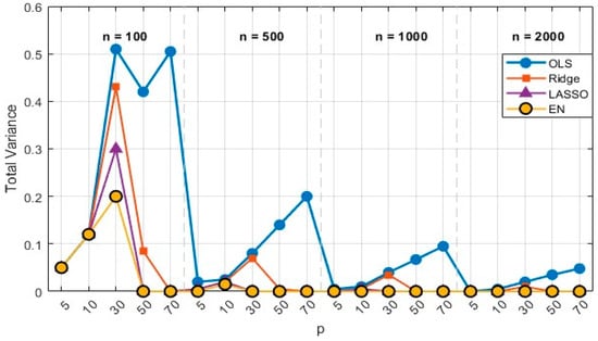
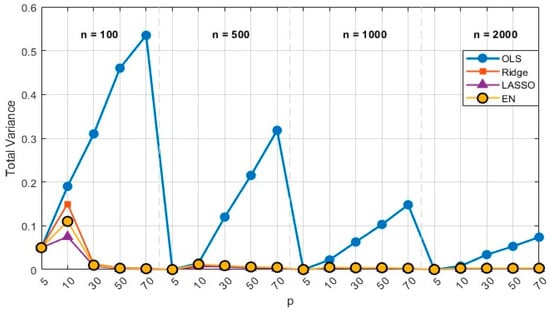
Figure 1 and Figure 2 provide graphical illustrations of the variance behavior of the estimators under moderate and severe multicollinearity levels, respectively. The variance of the OLS estimator is highly sensitive to both the correlation level and the value of p. In particular, for moderate values of p, OLS exhibits pronounced spikes in variance, which become even more severe under high correlation (G = 0.99). In contrast, LASSO and EN estimators exhibit values that are very close to each other across almost all p values, indicating a much more stable pattern. As p increases, and especially as the sample size grows, the variance of all estimators tends to decrease, and the differences between them become less pronounced. To enhance visual clarity and facilitate comparison among the estimators, the vertical axis is limited to the range [0, 0.6]. Therefore, a small number of variance values exceeding 0.6 fall outside the displayed range.
Figure 1.
Variance of estimators for G = 0.50 across different n and p values.
Figure 2.
Variance of estimators for G = 0.99 across different n and p values.
3.2. Real Data Application
The predictive performances of the OLS, ridge, LASSO, and EN estimators are evaluated using MSPE, RMSE, MAE, and R2 measures. MSPE is computed using the entire dataset, whereas the other performance metrics are evaluated on the test set. The number of observations in the test dataset is denoted by m. RMSE is defined as RMSE = and measures the average magnitude of prediction errors while assigning greater weight to large deviations. MAE is calculated as MAE = and represents the average absolute difference between observed and predicted values. The coefficient of determination is given by R2 = where denotes the mean of the observed values, and it indicates the proportion of variability in the dependent variable explained by the model. Lower RMSE and MAE values and higher R2 values indicate better predictive performance.
Table 7 presents the coefficient estimates obtained from the California Housing Dataset. While the estimated coefficients generally retain the same direction of effect across the estimators, their magnitudes differ considerably, reflecting the varying degrees of regularization imposed by ridge regression, LASSO, and EN.
Table 7.
Parameter estimates for the California Housing Dataset.
As shown in Table 8, the LASSO estimator exhibits superior predictive performance according to the test-set evaluation metrics. In particular, it produces the lowest RMSE and MAE values, while also yielding the highest R2 value. In contrast, OLS shows the weakest performance. These findings suggest that regularization-based methods, particularly LASSO, appear to be more effective in improving predictive accuracy and stability than the classical OLS estimator. Furthermore, although the EN estimator yields the lowest MSPE value, this does not substantially alter the overall comparative assessment, as MSPE reflects performance over the entire dataset, whereas RMSE, MAE, and R2 are computed on the test set. This difference accounts for the variation in ranking across evaluation criteria.
Table 8.
Performance metrics for the California house dataset.
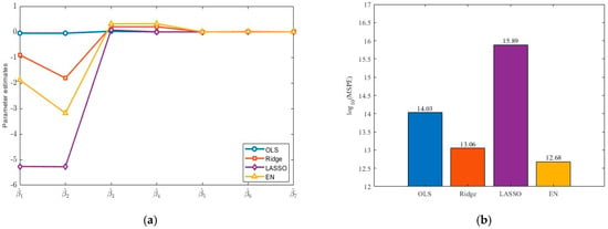
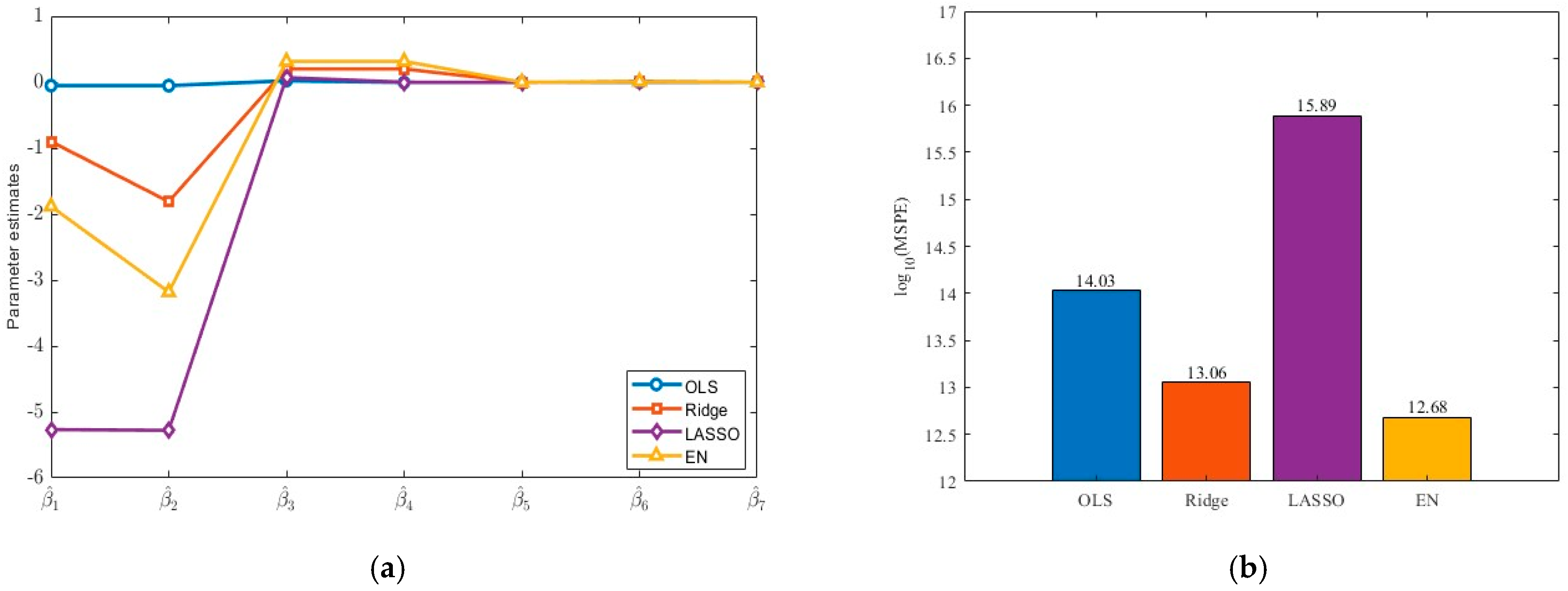
To complement the tabular analysis, Figure 3 presents a graphical illustration of the results, highlighting differences among the estimators in terms of coefficient behavior and predictive accuracy. Figure 3a compares the coefficient estimates obtained from the OLS, ridge, LASSO, and EN estimators, excluding the intercept term for improved visualization. Although the estimated coefficients generally preserve the same direction of effect across the estimators, noticeable differences are observed in their magnitudes due to the varying degrees of regularization. In particular, the coefficients associated with and exhibit the largest absolute values across all methods, indicating that these predictors have the strongest influence on housing prices. Ridge regression shrinks all coefficients toward zero while retaining every predictor in the model. LASSO applies stronger shrinkage and sets the coefficient exactly to zero, thereby performing variable selection. EN produces coefficient estimates that generally lie between those of ridge regression and LASSO, reflecting its hybrid regularization structure. Overall, the figure illustrates that regularization reduces coefficient variability while preserving the main patterns of association between the independent variables and the dependent variable. Figure 3b, on the other hand, compares the estimators in terms of MSPE values, providing an evaluation of their predictive performance. A logarithmic scale is used to appropriately accommodate the large differences in magnitude among the MSPE values across the considered estimators.
Figure 3.
Comparative results on the California Housing Dataset: (a) Estimated regression coefficients. (b) Log MSPEs across regression estimators.
The results indicate that the EN estimator achieves the lowest prediction error among the considered estimators. Ridge regression also demonstrates strong, stable performance with low MSPE values, whereas OLS yields substantially higher errors. Although LASSO effectively performs variable selection, it suffers from severe underfitting in this setting, leading to weaker predictive accuracy. In contrast, by retaining more information through coefficient shrinkage, ridge regression and EN achieve superior results. Specifically, EN provides a well-balanced trade-off between model flexibility and regularization, proving its effectiveness for this dataset.
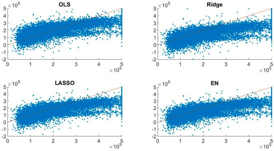
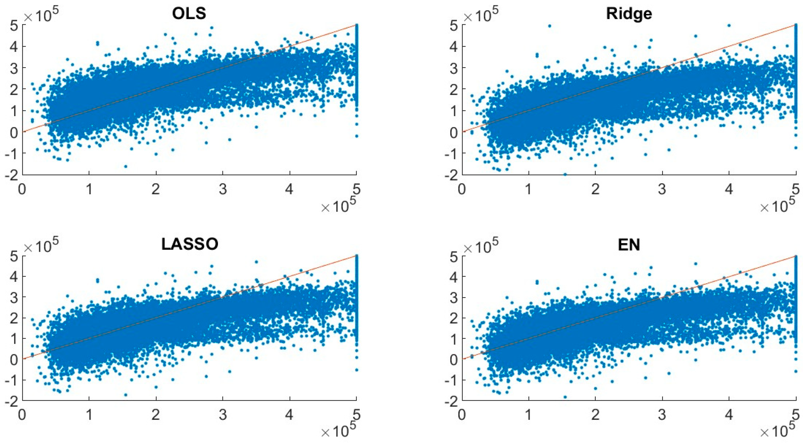
Figure 4 compares the observed house values with the predicted values obtained from the regression estimators. In each panel, the horizontal axis represents the observed values () and the vertical axis represents the predicted values (). Compared with OLS, the penalized regression estimators produce more stable prediction patterns, while the OLS estimator exhibits greater dispersion, suggesting a stronger influence of multicollinearity on prediction accuracy.
Figure 4.
Comparison between observed and predicted house values for the competing regression estimators.
4. Discussion
In empirical housing data, independent variables are often highly correlated, leading to multicollinearity problems that adversely affect the stability and predictive reliability of conventional regression models. The findings of this study demonstrate that regularization-based estimators provide substantial advantages over OLS under such conditions. Both the simulation study and the California Housing Dataset analysis indicate that ridge regression, LASSO, and EN achieve more stable parameter estimates and improved predictive performance when strong correlations exist among independent variables. Furthermore, the simulation results show that estimator performance depends on both the severity of multicollinearity and the dimensionality of the dataset. While the differences among the estimators remain relatively small under moderate correlation levels, more pronounced distinctions emerge as the correlation structure becomes stronger and the number of independent variables increases.
Among the competing regularization methods, LASSO performs particularly well in several simulation scenarios due to its ability to reduce variance through sparse coefficient estimation. By shrinking some coefficients exactly to zero, LASSO simplifies the model structure and performs automatic variable selection. However, the empirical results suggest that aggressive shrinkage may remove informative predictors in highly correlated datasets, leading to reduced predictive accuracy. Ridge regression, on the other hand, stabilizes coefficient estimates by shrinking all regression coefficients toward zero without excluding variables from the model. This characteristic improves estimation stability while preserving the contribution of all independent variables. Moreover, the simulation design assumes a sparse coefficient structure, where only a subset of the independent variables is associated with nonzero regression coefficients. Under such settings, methods capable of variable selection may have an advantage, which helps explain the strong performance of LASSO observed across many scenarios.
The empirical findings further indicate that EN provides the strongest overall predictive performance. By combining the L1 and L2 penalties, EN balances coefficient shrinkage and variable selection, thereby achieving improved prediction accuracy while maintaining model stability.
The graphical analyses support the numerical findings reported in the Results section. The coefficient comparison plots highlight the differences in coefficient magnitudes across the competing estimators and illustrate the shrinkage effect induced by regularization. Furthermore, the observed-versus-predicted plots provide a visual assessment of predictive performance across the competing estimators and complement the quantitative evaluation based on MSPE.
The findings obtained in this study are generally consistent with previous research emphasizing the benefits of regularization methods in the presence of multicollinearity. Earlier studies reported that ridge regression improves estimation stability by reducing variance [18], whereas LASSO performs effective variable selection through coefficient shrinkage [19]. More recent studies have shown that EN is particularly effective when groups of highly correlated independent variables are present [20]. The results from both the simulation study and the California Housing Dataset are consistent with these observations, suggesting that EN may exhibit a balanced performance between predictive accuracy and model stability.
Overall, the simulation and empirical analyses suggest that no single estimator is universally optimal under all conditions. Rather, the choice of estimator should depend on the degree of multicollinearity, the dimensionality of the dataset, and the performance criterion of primary interest. In the simulation study, LASSO generally exhibits lower total variance across many scenarios, whereas EN becomes more competitive under stronger multicollinearity. In the California Housing application, LASSO performs better according to the test-set evaluation metrics (RMSE, MAE, and R2), while EN achieves the lowest overall MSPE. These differences arise from the fact that RMSE, MAE, and R2 are computed on the test set, whereas MSPE is based on the full dataset and therefore reflects a different aspect of generalization performance.
5. Conclusions
This study investigates the predictive performance of OLS, ridge, LASSO, and EN estimators in the presence of multicollinearity using a comprehensive simulation framework and the California Housing Dataset as a real-world application. The simulation design systematically varies sample size, dimensionality, and correlation structure to assess estimator behavior under controlled and increasingly complex conditions, while the empirical analysis provides evidence from a practical high-dimensional regression setting.
The results consistently demonstrate that multicollinearity undermines the stability and predictive reliability of the OLS estimator, with effects becoming more pronounced in high-dimensional and highly correlated environments. In contrast, regularization-based methods substantially mitigate these issues by imposing coefficient shrinkage, thereby improving both estimation stability and out-of-sample predictive performance.
Comparative evidence further reveals that estimator performance is inherently data-dependent and driven by the interaction between dimensionality and correlation strength. In the empirical application, LASSO achieves the most favorable test-set performance according to RMSE, MAE, and R2, whereas EN yields the lowest overall MSPE. These findings indicate that the relative performance of the estimators depends on the evaluation criterion considered. The results further suggest that the relative advantages of LASSO and EN vary according to the correlation structure and the performance measure of interest.
Taken together, the simulation and empirical results provide strong empirical support for the use of regularization techniques in regression settings characterized by multicollinearity. Overall, the results demonstrate that regularization-based estimators offer effective alternatives to OLS, with the choice of estimator depending on the characteristics of the data and the performance criterion of primary interest.
Although the findings provide useful insights into the behavior of OLS, ridge, LASSO, and EN estimators under multicollinearity, several limitations should be acknowledged. First, the empirical analysis is based solely on the California Housing Dataset. Although this dataset is widely used in regression studies, the results may not fully generalize to datasets with different characteristics, distributions, or correlation structures. Second, the study focuses on classical and regularization-based linear regression methods and does not include comparisons with modern machine learning approaches such as Random Forest, XGBoost, LightGBM, or Neural Networks. Therefore, the conclusions should be interpreted within the scope of linear predictive modeling. Third, the simulation results depend on the selected experimental settings, including the sample sizes, numbers of independent variables, and correlation levels considered in the study. Different simulation designs may lead to different relative performances of the estimators. In particular, the use of a sparse coefficient structure in the simulation design may influence the relative performance of shrinkage-based estimators, and alternative dense settings may yield different comparative results, especially for ridge regression. Finally, although multiple evaluation metrics are employed, additional performance measures, alternative validation strategies, and formal statistical inference could provide further insights into model behavior. Future research may extend the analysis to other real-world datasets, alternative correlation structures, and more advanced predictive modeling techniques, as well as the selection of the EN mixing parameter through cross-validation or grid search procedures.
Author Contributions
Both authors contributed equally to all stages of the study, including conceptualization, data analysis, and manuscript writing. All authors have read and agreed to the published version of the manuscript.
Funding
This research received no external funding.
Data Availability Statement
The original contributions presented in this study are included in the article. The datasets analyzed in this study are available in Kaggle at https://www.kaggle.com/datasets/dhirajnirne/california-housing-data (accessed on 12 May 2026).
Conflicts of Interest
The authors declare no conflicts of interest.
Abbreviations
The following abbreviations are used in this manuscript:
| OLS | Ordinary least squares |
| LASSO | Least absolute shrinkage and selection operator |
| EN | Elastic net |
| RSS | Residual sum of squares |
| VIF | Variance inflation factor |
| MSPE | Mean square prediction error |
| RMSE | Root mean squared error |
| MAE | Mean absolute error |
References
- Ahmad, M.H.; Adnan, R.; Adnan, N. A comparative study on some methods for handling multicollinearity problems. Matematika 2006, 22, 109–119. [Google Scholar]
- Kroll, C.N.; Song, P. Impact of multicollinearity on small sample hydrologic regression models. Water Resour. Res. 2013, 49, 3756–3769. [Google Scholar] [CrossRef] [Scilit]
- Stewart, G.W. Collinearity and least squares regression. Stat. Sci. 1987, 2, 68–84. [Google Scholar] [CrossRef] [Scilit]
- Sharma, H.; Harsora, H.; Ogunleye, B. An optimal house price prediction algorithm: XGBoost. Analytics 2024, 3, 30–45. [Google Scholar] [CrossRef] [Scilit]
- Mullainathan, S.; Spiess, J. Machine learning: An applied econometric approach. J. Econ. Perspect. 2017, 31, 87–106. [Google Scholar] [CrossRef] [Scilit]
- Mora-Garcia, R.-T.; Cespedes-Lopez, M.-F.; Perez-Sanchez, V.R. Housing price prediction using machine learning algorithms in COVID-19 times. Land 2022, 11, 2100. [Google Scholar] [CrossRef] [Scilit]
- Abdelwahab, M.M.; Abonazel, M.R.; Hammad, A.T.; El-Masry, A.M. Modified two-parameter Liu estimator for addressing multicollinearity in the poisson regression model. Axioms 2024, 13, 46. [Google Scholar] [CrossRef] [Scilit]
- Nayem, H.M.; Aziz, S.; Kibria, B.M.G. Evaluating estimator performance under multicollinearity: A trade-off between MSE and accuracy in logistic, lasso, elastic net, and ridge regression with varying penalty parameters. Stats 2025, 8, 45. [Google Scholar] [CrossRef] [Scilit]
- Alharthi, M.F.; Akhtar, N. Modified two-parameter ridge estimators for enhanced regression performance in the presence of multicollinearity: Simulations and medical data applications. Axioms 2025, 14, 527. [Google Scholar] [CrossRef] [Scilit]
- An, J.; Park, J.; Yeon, S.; Oh, C.; Lee, B.; Jung, W.; Yun, J.; Oh, H.J. Machine learning-based prediction of Coagulant dosing in drinking water treatment plants using polynomial regression with lasso regularization. Processes 2025, 13, 3829. [Google Scholar] [CrossRef] [Scilit]
- Xin, S.J.; Khalid, K. Modelling house price using ridge regression and lasso regression. Int. J. Eng. Technol. 2018, 7, 498–501. [Google Scholar] [CrossRef] [Scilit]
- Nayem, H.M.; Aziz, S.; Kibria, B.M.G. Comparison among ordinary least squares, ridge, lasso, and elastic net estimators in the presence of outliers: Simulation and application. Int. J. Stat. Sci. 2024, 24, 25–48. [Google Scholar] [CrossRef] [Scilit]
- Gabauer, D.; Gupta, R.; Marfatia, H.A.; Miller, S.M. Estimating US housing price network connectedness: Evidence from dynamic Elastic Net, Lasso, and ridge vector autoregressive models. Int. Rev. Econ. Financ. 2024, 89, 349–362. [Google Scholar] [CrossRef] [Scilit]
- Preethi; Murthy, D.H.R.; Hiremani, V.; Devadas, R.M.; Sapna, R. Optimizing polynomial and regularization techniques for enhanced housing price prediction accuracy. SN Comput. Sci. 2025, 6, 96. [Google Scholar] [CrossRef] [Scilit]
- Zeng, Z. Using Linear Regression, Ridge Regression, Lasso Regression, and Elastic Net Regression for Predicting Real Estate Price. In Proceedings of the 2nd International Conference on Data Science and Engineering (ICDSE); SCITEPRESS: Setúbal Municipality, Portugal, 2025. [Google Scholar] [CrossRef] [Scilit]
- Elkhidir, E.; Patel, T.; Rotimi, J.O.B. Predictive modelling for residential construction demands using ElasticNet Regression. Buildings 2025, 15, 1649. [Google Scholar] [CrossRef] [Scilit]
- Xia, H. Lasso’s application in Chinese housing prices. Commun. Stat. Theory Methods 2026, 55, 2465–2476. [Google Scholar] [CrossRef] [Scilit]
- Hoerl, A.E.; Kennard, R.W. Ridge regression: Biased estimation for nonorthogonal problems. Technometrics 1970, 12, 55–67. [Google Scholar] [CrossRef]
- Tibshirani, R. Regression shrinkage and selection via the lasso. J. R. Stat. Soc. Ser. B 1996, 58, 267–288. [Google Scholar] [CrossRef] [Scilit]
- Zou, H.; Hastie, T. Regularization and Variable Selection via the Elastic Net. J. R. Stat. Soc. Ser. B 2005, 67, 301–320. [Google Scholar] [CrossRef] [Scilit]
- Dormann, C.F.; Elith, J.; Bacher, S.; Buchmann, C.; Carl, G.; Carré, G.; Marquéz, J.R.G.; Gruber, B.; Lafourcade, B.; Leitão, P.J.; et al. Collinearity: A review of methods to deal with it and a simulation study evaluating their performance. Ecography 2013, 36, 27–46. [Google Scholar] [CrossRef] [Scilit]
- Hebiri, M.; Lederer, J. How correlations influence lasso prediction. IEEE Trans. Inf. Theory 2012, 59, 1846–1854. [Google Scholar] [CrossRef] [Scilit]
- Hastie, T.; Tibshirani, R.; Friedman, J. The Elements of Statistical Learning, 2nd ed.; Springer: New York, NY, USA, 2009. [Google Scholar]
- Fu, W.J. Penalized regressions: The bridge versus the lasso. J. Comput. Graph. Stat. 1998, 7, 397–416. [Google Scholar] [CrossRef] [Scilit]
- Muthukrishnan, R.; Rohini, R. LASSO: A Feature Selection Technique in Predictive Modeling for Machine Learning. In Proceedings of the International Conference on Advances in Computer Applications (ICACA), Coimbatore, India, 24 October 2016. [Google Scholar] [CrossRef] [Scilit]
- Hans, C. Elastic net regression modeling with the orthant normal prior. J. Am. Stat. Assoc. 2011, 106, 1383–1393. [Google Scholar] [CrossRef] [Scilit]
- Kaggle. Available online: https://www.kaggle.com/datasets/dhirajnirne/california-housing-data (accessed on 5 February 2026).
- Bun, M.J.G.; Harrison, T.D. OLS and IV estimation of regression models including endogenous interaction terms. Econom. Rev. 2019, 38, 814–827. [Google Scholar] [CrossRef] [Scilit]
- Yang, H.; Chang, X. A new two-parameter estimator in linear regression. Commun. Stat. Theory Methods 2010, 39, 923–934. [Google Scholar] [CrossRef] [Scilit]
- James, G.; Witten, D.; Hastie, T.; Tibshirani, R. An Introduction to Statistical Learning: With Applications in R, 2nd ed.; Springer: New York, NY, USA, 2021. [Google Scholar] [CrossRef] [Scilit] [PubMed]
- Algamal, Z.Y. Shrinkage parameter selection via modified cross-validation approach for ridge regression model. Commun. Stat. Simul. Comput. 2020, 49, 1922–1930. [Google Scholar] [CrossRef] [Scilit]
- Nakatsu, R.T. Validation of machine learning ridge regression models using Monte Carlo, bootstrap, and variations in cross-validation. J. Intell. Syst. 2023, 32, 20220224. [Google Scholar] [CrossRef] [Scilit]
- Hoerl, R.W. Ridge regression: A historical context. Technometrics 2020, 62, 420–425. [Google Scholar] [CrossRef] [Scilit]
- Lukman, A.F.; Ali, E. Contraction ridge estimator: Simulation and application to economic data. Comp. Econ. 2025, 1–25. [Google Scholar] [CrossRef] [Scilit]
- Yi, C.; Huang, J. Semismooth newton coordinate descent algorithm for elastic-net penalized huber loss regression and quantile regression. J. Comput. Graph. Stat. 2017, 26, 547–557. [Google Scholar] [CrossRef] [Scilit]
- Wright, S.J. Coordinate descent algorithms. Math. Program. 2015, 151, 3–34. [Google Scholar] [CrossRef] [Scilit]
- Ranstam, J.; Cook, J.A. LASSO regression. Br. J. Surg. 2018, 105, 1348. [Google Scholar] [CrossRef] [Scilit]
- Hastie, T.; Tibshirani, R.; Wainwright, M. Statistical Learning with Sparsity: The Lasso and Generalizations, 1st ed.; Chapman and Hall/CRC: Boca Raton, FL, USA, 2015. [Google Scholar] [CrossRef] [Scilit]
- Xu, Q.F.; Ding, X.H.; Jiang, C.X.; Yu, K.M.; Shi, L. An elastic-net penalized expectile regression with applications. J. Appl. Stat. 2021, 48, 2205–2230. [Google Scholar] [CrossRef] [Scilit] [PubMed]
- Raymaekers, J.; Rousseeuw, P.J. The cellwise minimum covariance determinant estimator. J. Am. Stat. Assoc. 2024, 119, 2610–2621. [Google Scholar] [CrossRef] [Scilit]
- Steland, A. Shrinkage for covariance estimation: Asymptotics, confidence intervals, bounds and applications in sensor monitoring and finance. Stat. Pap. 2018, 59, 1441–1462. [Google Scholar] [CrossRef] [Scilit]

Disclaimer/Publisher’s Note: The statements, opinions and data contained in all publications are solely those of the individual author(s) and contributor(s) and not of MDPI and/or the editor(s). MDPI and/or the editor(s) disclaim responsibility for any injury to people or property resulting from any ideas, methods, instructions or products referred to in the content. |
© 2026 by the authors. Licensee MDPI, Basel, Switzerland. This article is an open access article distributed under the terms and conditions of the Creative Commons Attribution (CC BY) license.