Complex Double Interface Dynamics in Time-Fractional Models: Computational Analysis of Meshless and Multi-Resolution Techniques

Abstract

Time-fractional interface problems, found in heat transfer with discontinuous conductivities and fluid flows with surface tension forces, are challenging due to irregular interfaces and the history-dependent nature of fractional derivatives. This paper presents two numerical methods for simulating time-fractional double interface problems. The first method uses the Haar wavelet collocation technique, while the second relies on a meshless approach with radial basis functions. The fractional derivatives are replaced with the Caputo sense, the resulting first-order time derivatives are handled using the finite difference method, and the spatial operator is approximated using the two proposed methods. Gauss elimination is used to solve linear problems. Quasi-Newton linearization method is used for nonlinear problems. Both methods accommodate constant and variable coefficients, handling discontinuities and singularities in both solutions and coefficients. To evaluate the effectiveness of the proposed methods, numerical experiments are carried out. The accuracy of each method is quantified using the $L_{\infty }$ error norm, and a comparative analysis highlights the validity and advantages of the approaches. Moreover, the proposed schemes are rigorously analyzed to establish their stability, and the existence and uniqueness of the solutions.

1. Introduction

Interfaces often arise in situations where a domain is divided into subdomains, each possessing distinct physical or mathematical properties, such as fluid flow through composite materials or multi-layered structures. Common examples include heat conduction in heterogeneous materials (a parabolic problem) and wave propagation in composite media (a hyperbolic problem). Since exact analytical solutions are rarely available, conventional numerical methods frequently face challenges in solving such interface problems [1,2]. The primary reason is that solutions near interfaces may exhibit irregular or non-smooth behavior, which can significantly reduce the accuracy and stability of standard techniques like the finite difference method (FDM) and finite element method (FEM) [3,4].

Interface problems have drawn the attention of mathematicians and physicists alike in recent years, leading to the establishment of numerous effective computing techniques. Numerous fields, such as the study of materials, system biology, ecological science, and radiation propagation, deal with such problems [5,6]. Numerous numerical techniques have been put out in the literature. To solve elliptic interface equations, for instance, Babuska adopted FDM [7]. Haar wavelet collocation method (HWCM) and meshfree approaches were used by Aziz et al. to tackle elliptic and parabolic interface problems [8,9]. For hyperbolic interface models, Asif et al. employed HWCM [10]. They then expanded it to find approximate solutions for the telegraph interface equation [11]. Rana et al. used HWCM to study the challenges of the elliptic and parabolic interface of advection-diffusion reaction [12]. Asif and Faisal applied the HWCM to the telegraph interface model with a single interface [13], while employing the meshfree approaches for the nonlinear telegraph equation with a single interface [14] and for hyperbolic models involving both single and double interfaces [15]. To handle the Stokes system with interfaces, Ahmad et al. utilized local meshless schemes [16], and later used the same method to elliptic interface equations [17]. Recent studies have explored soliton solutions, traveling waves, and stability analysis in various nonlinear evolution equations using analytical and numerical techniques [18,19,20,21,22].

Fractional calculus dates back to the beginnings of classical calculus. In a letter to L’Hôpital in 1695, Leibniz proposed the intriguing concept of derivatives of non-integer order. During the nineteenth century, Liouville and Riemann formalized this idea and demonstrated its effectiveness in modeling electrochemical systems [23]. Their work highlighted that memory and hereditary effects can be naturally incorporated through fractional derivatives and integrals, often providing more accurate and efficient models than conventional integer-order derivatives. Fractional differential equations (FDEs) are now widely employed to study a variety of real-world phenomena, including the flow and deformation of complex materials, time-dependent changes in material properties under stress, stochastic particle motion, and biological system dynamics. Applications include modeling the response of living cells and polymers to stress, predicting pollutant transport through soil and rock, evaluating disease progression, and designing more precise and reliable control systems. By capturing subtle dynamics often overlooked by classical models, fractional calculus has emerged as a powerful and versatile tool across science and engineering disciplines [24,25,26].

The widespread and increasing use of FDEs has resulted in the development of numerous numerical approaches to determine approximate solutions. Zada et al. used the HWCM for FPDEs [27]. Mehnaz et al. first proposed a meshless technique for time FPDEs [28] and later developed a local meshless strategy for space FPDEs [29]. Manzoor and Siraj applied a meshless spectral approach to solve the time-fractional KdV equation [30]. Haifa and Carlo used Chebyshev cardinal functions to estimate the solutions of temporal FPDEs [31]. Rehma and Banan developed an adaptive technique for fractional elliptic interface models [32], whereas Wang et al. used space-time FET to tackle time-fractional diffusion problems with interfaces [33].

Haar wavelets (HWs) are a set of piecewise constants functions that take values of 0, 1, or $-1$ over subintervals of $x\in [a,b]$. They constitute a base that is orthonormal in the function space $L^2[a,b]$. HWs have gained popular in recent years due to the simplicity of use and efficiency in solving differential equations [34]. The HWCM has been widely explored for the analysis and numerical solution of linear and nonlinear systems, including time-delayed systems, integro-differential equations, and partial differential equations [35,36,37,38,39,40,41,42,43,44,45,46]. Because of their compact support and piecewise constant nature, HWs are especially well-suited for dealing with problems needing discontinuities or abruptly transitions. These features make HWCM an accurate and versatile solution for numerous applications, including control systems, signal processing, and financial modeling [47,48]. Higher-order HWCM have been employed in recent studies to enhance precision and convergence in solving differential equations [49,50].

Radial basis functions (RBFs) are frequently used to tackle a wide range of problems, including partial differential, integral, integro-differential, and fractional PDEs. Through the approximation of spatial derivatives, RBFs transform nonlinear or complex PDEs into linear systems, which proves especially advantageous for high-dimensional problems or domains with intricate shapes [28]. The adaptable nature of RBFs has led to applications in contemporary domains such as artificial intelligence, high-dimensional data approximation, computational mechanics, medical image reconstruction, computer vision, spatial data modeling, computer graphics, and robotics [51]. The origins of RBFs trace back to Hardy’s 1971 work, in which they were employed to approximate two-dimensional geographic surfaces [52]. Later, Kansa applied the RBF framework to tackle PDEs [53]. Further contributions by Franke and Schaback addressed critical theoretical aspects, such as ensuring convergence and uniqueness [54]; furthermore, the work of Hon et al. broadened RBF applications to include nonlinear differential equations, such as Burgers’ equation [55].

2. Governing Equations

In this study, we have concentrated on linear time-fractional double interface problems in one dimension (1D). The following is a representation of the problem

$${\displaystyle \frac{{\partial }^{\rho }\phi (\mathcal{x},t)}{\partial t^{\rho }}}=\nabla ·(\eta \nabla \phi )+\Phi ,0<\rho <1,t\ge t_0,\mathrm{in}\Omega ,$$

(1)

and the nonlinear time-fractional double interface is

$${\displaystyle \frac{{\partial }^{\rho }\phi (\mathcal{x},t)}{\partial t^{\rho }}}=\nabla ·(\eta \nabla \phi )+\mathcal{F}(\mathcal{x},t,\phi (\mathcal{x},t))+\Phi ,0<\rho <1,t\ge t_0,\mathrm{in}\Omega .$$

(2)

In Equations (1) and (2), the fractional time derivative ${\displaystyle \frac{{\partial }^{\rho }\varphi (\mathcal{x},t)}{\partial t^{\rho }}}$ is adopted in the Caputo sense with order $0<\rho <1$, where $\mathcal{F}(\mathcal{x},t,\phi (\mathcal{x},t))$ is a nonlinear term. The function $\Phi (\mathcal{x},t)$ serves as a source term, whereas $\eta (\mathcal{x})$ is a smoothly varying coefficient. This formulation will be used for $t\ge t_0$, where $t_0$ indicates the initial time, and $\mathcal{x}\in \Omega$, with $\Omega \subset \mathbb{R}$ for 1D problems. In this 1D example, the gradient operator simplifies to $\nabla =\left({\displaystyle \frac{\partial }{\partial \mathcal{x}}}\right)$.

A double interface at ${\theta }_1$ and ${\theta }_2$ splits the domain $\Omega$ into three subdomains. To represent this partitioning, the functions $\phi$, a, and $\Phi$ are defined independently in each subdomain.

$$\begin{array}{c}\hfill (\phi ,a,\Phi )=\left\{\begin{array}{cc}({\phi }^{+},a^{+},{\Phi }^{+})\hfill & \mathrm{in}{\Omega }^{+},\hfill \\ ({\phi }^0,a^0,{\Phi }^0)\hfill & \mathrm{in}{\Omega }^0,\hfill \\ ({\phi }^{-},a^{-},{\Phi }^{-})\hfill & \mathrm{in}{\Omega }^{-}.\hfill \end{array}\right.\end{array}$$

(3)

The boundary and initial conditions are

$$\begin{array}{cc}\hfill \phi (\mathcal{x},t)& =\chi ,(\mathcal{x},t)\in \partial \Omega \times (0,T_f],\hfill \\ \hfill \phi (\mathcal{x},0)& ={\varpi }_1,\mathcal{x}\in \Omega ,\hfill \\ \hfill {\phi }_t(\mathcal{x},0)& ={\varpi }_2,\mathcal{x}\in \Omega .\hfill \end{array}$$

(4)

At the two interfaces $\mathcal{x}={\theta }_1$ and $\mathcal{x}={\theta }_2$, the following conditions are imposed:

$$\begin{array}{ccc}\hfill {\left[\phi \right]}_{{\theta }_1}& =& {\phi }_1({\theta }_1,t)-{\phi }_2({\theta }_1,t)={\omega }_1({\theta }_1,t),\hfill \end{array}$$

(5)

$$\begin{array}{ccc}\hfill {\left[\eta {\phi }_{\mathcal{x}}\right]}_{{\theta }_1}& =& {\eta }^{+}({\theta }_1,t){\phi }_{1\mathcal{x}}({\theta }_1,t)-{\eta }^0({\theta }_1,t){\phi }_{2\mathcal{x}}({\theta }_1,t)={\nu }_1({\theta }_1,t),\hfill \end{array}$$

(6)

$$\begin{array}{ccc}\hfill {\left[\phi \right]}_{{\theta }_2}& =& {\phi }_2({\theta }_2,t)-{\phi }_3({\theta }_2,t)={\omega }_2({\theta }_2,t),\hfill \end{array}$$

(7)

$$\begin{array}{ccc}\hfill {\left[\eta {\phi }_{\mathcal{x}}\right]}_{{\theta }_2}& =& {\eta }^0({\theta }_2,t){\phi }_{2\mathcal{x}}({\theta }_2,t)-{\eta }^{-}({\theta }_2,t){\phi }_{3\mathcal{x}}({\theta }_2,t)={\nu }_2({\theta }_2,t).\hfill \end{array}$$

(8)

This study considers the spatial domain $\Omega$ as the interval $[0,1]$ for 1D problems to simplify the analysis. The domain is divided into three subregions as shown in Figure 1: ${\Omega }^{+}=[0,{\theta }_1]$, ${\Omega }^0=[{\theta }_1,{\theta }_2]$, and ${\Omega }^{-}=[{\theta }_2,1]$. The interfaces are located in the positions $\mathcal{x}={\theta }_1$ and $\mathcal{x}={\theta }_2$ without sacrificing generality.

Figure 1. One-dimensional diagram of double interfaces.

We first provide some fundamental definitions and notations pertaining to fractional derivatives in order to do the analysis that follows.

Definition 1.

The Caputo fractional derivative of order $\rho >0$ for a function $\phi (t)$, which is absolutely continuous on the interval $[0,T]$, is defined as

$${}^{C}D_t^{\rho }\phi (\mathcal{x},t)={\displaystyle \frac{1}{\Gamma (m-\rho )}}{\int }_0^t{\displaystyle \frac{{\phi }^{(m)}(\zeta )}{{(t-\zeta )}^{\rho -m+1}}}d\zeta .$$

(9)

This definition clearly indicates that the time-fractional model possesses the memory (history-dependent) property, since the fractional derivative at time t depends on the entire past history of the solution over the interval $[t_0,\mathcal{T}]$. In the present study, the memory begins from the initial time $t_0=0$; hence, the evolution of $\varphi (\mathcal{x},t)$ depends on its complete history from $t=0$ up to the current time t. This memory property is consistent with the standard interpretation of Caputo-type fractional operators as discussed in [56,57]. In this study, the Caputo time-fractional derivative is employed due to its suitability for physical and engineering applications. One of its main advantages is that it allows the use of classical integer-order initial conditions, which have clear physical interpretations. Moreover, the Caputo derivative effectively captures memory effects and nonlocal temporal dynamics, making it well suited for modeling time-fractional interface problems. These properties justify its selection over classical derivatives and other fractional definitions in the present computational framework.

3. The Main Objective of the Study

This work focuses on developing and examining reliable numerical techniques for one-dimensional time-fractional double interface problems, which are often complicated by discontinuous coefficients, non-smooth solutions, and the presence of memory effects. To address these challenges, two different approaches are proposed and systematically compared: HWCM and MQ-RBF. The Caputo fractional derivative is employed to capture the inherent memory and hereditary properties of fractional models, while advanced spatial approximation strategies are utilized to enhance stability, accuracy, and computational efficiency in the presence of multiple interfaces. By contrast with existing studies that primarily focus on single-interface or integer-order formulations, the present work provides a unified computational framework for time-fractional double interface problems and offers a detailed comparative assessment of HWCM and MQ-RBF methods. This enables a more faithful and robust numerical description of anomalous diffusion and complex material behavior.

The paper is structured as follows. Section 2 introduces the governing equation for the time-fractional double interface problem. In Section 4, we describe the numerical procedure, where the temporal approximation based on the Caputo fractional derivative is presented in Section 4.1. Section 4.2 focuses on RBFs and their role in the meshless framework. Spatial discretization is discussed in Section 4.3, where the MCM is presented. Section 4.4 covers the HWs, and Section 4.5 develops the HWCM for tackling time-fractional double interface problems. Section 5 presents a discussion on the existence and uniqueness of the solution. The stability analysis of the proposed method is discussed in Section 6. Section 7 provides numerical validation to show the precision and effectiveness of the proposed techniques. Finally, Section 8 offers final remarks and suggestions for future research.

4. Numerical Procedure

In this section, we first present the temporal discretization scheme for the time-fractional derivative, formulated in the Caputo sense, to accurately approximate the fractional term. Subsequently, we discuss the implementation of the MQ-RBF and HWCM for solving time-fractional double interface problems.

4.1. Temporal Approximation Using Caputo Derivative

This section aims to derive the Caputo fractional derivative for $\rho \in (0,1)$, which is described by [58,59]

$${\displaystyle \frac{{\partial }^{\rho }\phi (\mathcal{x},t^{m+1})}{\partial t^{\rho }}}=\left\{\begin{array}{cc}{\displaystyle \frac{1}{\Gamma \left(1-\rho \right)}}\underset{0}{\overset{t}{\int }}{\phi }^{\prime }(t){\left(t-\zeta \right)}^{-\rho }d\zeta ,\hfill & 0<\rho <1.\hfill \\ \hfill & \\ {\displaystyle \frac{\partial \phi }{\partial t}},\hfill & \rho =1.\hfill \end{array}\right.$$

Differentiating at $t=t^{m+1}$, we obtain

$${\displaystyle \frac{{\partial }^{\rho }\phi (\mathcal{x},t^{m+1})}{\partial t^{\rho }}}={\displaystyle \frac{1}{\Gamma (1-\rho )}}\underset{0}{\overset{t^{m+1}}{\int }}{\phi }^{\prime }(t){\left(t^{m+1}-\zeta \right)}^{-\rho }d\zeta .$$

For a uniform temporal grid $0=t_0<t_1<\cdots <t_{m+1}$, the integral can be split over the subintervals as

$$\Rightarrow {\displaystyle \frac{{\partial }^{\rho }\phi (\mathcal{x},t^{m+1})}{\partial t^{\rho }}}={\displaystyle \frac{1}{\Gamma (1-\rho )}}\sum _{k=0}^m\underset{t^k}{\overset{t^{k+1}}{\int }}{\phi }^{\prime }(t){\left(t^{m+1}-\zeta \right)}^{-\rho }d\zeta .$$

Now, we apply the FDM to estimate ${\displaystyle \frac{{\partial }^{m+1}\phi }{\partial t^{m+1}}}$, as we pursue,

$${\displaystyle \frac{\partial \phi (\mathcal{x},t^{m+1})}{\partial t}}={\displaystyle \frac{{\phi }^{k+1}-{\phi }^k}{dt}}+\mathcal{O}(dt).$$

Then,

$${\displaystyle \frac{{\partial }^{\rho }\phi (\mathcal{x},t^{m+1})}{\partial t^{\rho }}}\approx {\displaystyle \frac{1}{\Gamma (1-\rho )}}\sum _{k=0}^m\underset{t^k}{\overset{t^{k+1}}{\int }}{\displaystyle \frac{{\phi }^{k+1}-{\phi }^k}{dt}}{\left(t^{m+1}-\zeta \right)}^{-\rho }d\zeta +\mathcal{O}(d{t}^{2-\rho }).$$

$${\displaystyle \frac{{\partial }^{\rho }\phi (\mathcal{x},t^{m+1})}{\partial t^{\rho }}}=a_0\sum _{k=0}^m{b}_k\left({\phi }^{m-k+1}-{\phi }^{m-k}\right)+\mathcal{O}(d{t}^{2-\rho }).$$

where $b_k={(k+1)}^{1-\rho }-k^{1-\rho }$,$k=0,1,\dots ,m$ and $a_0={\displaystyle \frac{d{t}^{-\rho }}{\Gamma (2-\rho )}}$.

Finally, we can express it in a more refined form as follows:

$${\displaystyle \frac{{\partial }^{\rho }\phi (\mathcal{x},t^{m+1})}{\partial t^{\rho }}}=\left\{\begin{array}{cc}\hfill & \\ a_0\left({\phi }^{m+1}-{\phi }^m\right)+a_0{\displaystyle \sum _{k=1}^m}{b}_k\left({\phi }^{m-k+1}-{\phi }^{m-k}\right),\hfill & n\ge 1,\hfill \\ \hfill & \\ a_0\left({\phi }^1-{\phi }^0\right),\hfill & m=0.\hfill \end{array}\right.$$

(10)

Replacing the fractional derivative in the time-fractional double interface problems with its Caputo form and applying the FDM derived above, we substitute it in Equation (1),

$$a_0\left({\phi }^{m+1}-{\phi }^m\right)+a_0\sum _{k=1}^m{b}_k\left({\phi }^{m-k+1}-{\phi }^{m-k}\right)=\nabla ·(\eta \nabla \phi )+\Phi ,0<\rho <1,t\ge t_0,\mathrm{in}\Omega ,$$

(11)

and Equation (2),

$$\begin{array}{cc}\hfill & a_0\left({\phi }^{m+1}-{\phi }^m\right)+a_0\sum _{k=1}^m{b}_k\left({\phi }^{m-k+1}-{\phi }^{m-k}\right)\hfill \\ \hfill & =\nabla ·(\eta \nabla \phi )+\mathcal{F}(\mathcal{x},t,\phi (\mathcal{x},t))+\Phi ,0<\rho <1,t\ge t_0,\mathrm{in}\Omega .\hfill \end{array}$$

(12)

4.2. Radial Basis Functions

A function $\psi :{\mathbb{R}}^d\to \mathbb{R}$ is termed a radial function if it admits the representation $\psi (\mathcal{x})=\psi \left(\parallel \mathcal{x}\parallel \right)$ where $\psi :[0,\infty )\to \mathbb{R}$ is a single variable function and $\parallel ·\parallel$ denotes a norm in ${\mathbb{R}}^d$. In most cases, this norm is taken as the Euclidean norm, although other distance measures can also be utilized. This means the value of $\psi (\mathcal{x})$ is governed only by the length of the vector $\mathcal{x}$, not on its direction.

By letting $r=\parallel \mathcal{x}\parallel$, the function $\psi (r)$ is known as a RBF, described for $r\ge 0$ under the Euclidean norm. Many RBFs involve a positive parameter $ϵ>0$, often referred to as the shape parameter. In the present study, we employ the multiquadric RBF (MQ-RBF) to construct a numerical scheme for solving time-fractional double interface problems, where the MQ-RBF is described as

$$\psi (r)=\sqrt{1+{(ϵr)}^2},ϵ>0.$$

(13)

In MQ-RBF, the shape parameter $ϵ$ plays a crucial role in balancing accuracy, numerical stability, and conditioning of the resulting algebraic system. Smaller values of $\epsilon$ may improve accuracy due to increased flatness of the basis functions but often lead to severe ill-conditioning, whereas larger values enhance stability at the cost of reduced accuracy.

Since no universal optimal theoretical value of $ϵ$ exists, its selection is problem-dependent and commonly guided by empirical evidence reported in the literature. To assess the sensitivity of the proposed scheme, numerical experiments were conducted for different values of $ϵ$. The corresponding results are presented in tabular form and illustrated through figures for various shape parameter values. The results show that moderate values of $ϵ$ provide stable and accurate solutions, while extreme values adversely affect conditioning or accuracy. Accordingly, a fixed moderate value of $ϵ$ is adopted throughout the computations.

4.3. Meshless Collocation Method for Time-Fractional Double Interface Problems

The 1st subinterval ${\Omega }^{+}=[0,{\theta }_1]$ is classified into ${\mathcal{M}}_1$ subintervals determined by points $0={\mathcal{x}}_1<{\mathcal{x}}_2<\cdots <{\mathcal{x}}_{{\mathcal{M}}_1+1}={\theta }_1$, the 2nd subinterval ${\Omega }^0=[{\theta }_1,{\theta }_2]$ is divided into ${\mathcal{M}}_2$ subintervals using points ${\theta }_1={\mathcal{x}}_{{\mathcal{M}}_1+1}<{\mathcal{x}}_{{\mathcal{M}}_1+2}<\cdots <{\mathcal{x}}_{{\mathcal{M}}_2+1}={\theta }_2$, and the 3rd subinterval ${\Omega }^{-}=[{\theta }_2,1]$ is separated into ${\mathcal{M}}_3$ partitions formed by points ${\theta }_2={\mathcal{x}}_{{\mathcal{M}}_2+1}<{\mathcal{x}}_{{\mathcal{M}}_2+2}<\cdots <{\mathcal{x}}_{\mathcal{N}}$ where $\mathcal{N}={\mathcal{M}}_1+{\mathcal{M}}_2+{\mathcal{M}}_3+1$.

In the context of meshfree approaches to time-fractional double interface problems, the estimation on the 1st partition segment ${\Omega }^{+}=[0,{\theta }_1]$ is

$${\phi }_1(\mathcal{x},t)=\sum _{i=1}^{{\mathcal{M}}_1+1}{\lambda }_i\varphi (|\mathcal{x}-{\mathcal{x}}_i|),\mathcal{x}\in {\Omega }^{+},$$

(14)

differentiating Equation (14) w.r.t. $\mathcal{x}$, we get

$${\phi }_{1\mathcal{x}}(\mathcal{x},t)=\sum _{i=1}^{{\mathcal{M}}_1+1}{\lambda }_i{\varphi }^{\prime }(|\mathcal{x}-{\mathcal{x}}_i|),\mathcal{x}\in {\Omega }^{+},$$

(15)

again differentiating Equation (15) w.r.t. $\mathcal{x}$, we get

$${\phi }_{1\mathcal{x}\mathcal{x}}(\mathcal{x},t)=\sum _{i=1}^{{\mathcal{M}}_1+1}{\lambda }_i{\varphi }^{″}(|\mathcal{x}-{\mathcal{x}}_i|),\mathcal{x}\in {\Omega }^{+}.$$

(16)

For the 2nd subinterval ${\Omega }^0=[{\theta }_1,{\theta }_2]$, the estimation is

$${\phi }_2(\mathcal{x},t)=\sum _{i={\mathcal{M}}_1+1}^{{\mathcal{M}}_1+{\mathcal{M}}_2+1}{\gamma }_i\varphi (|\mathcal{x}-{\mathcal{x}}_i|),\mathcal{x}\in {\Omega }^0,$$

(17)

differentiating Equation (17) w.r.t. $\mathcal{x}$, we get

$${\phi }_{2\mathcal{x}}(\mathcal{x},t)=\sum _{i={\mathcal{M}}_1+1}^{{\mathcal{M}}_1+{\mathcal{M}}_2+1}{\gamma }_i{\varphi }^{\prime }(|\mathcal{x}-{\mathcal{x}}_i|),\mathcal{x}\in {\Omega }^0,$$

(18)

again differentiating Equation (18) w.r.t. $\mathcal{x}$, we get

$${\phi }_{2\mathcal{x}\mathcal{x}}(\mathcal{x},t)=\sum _{i={\mathcal{M}}_1+1}^{{\mathcal{M}}_1+{\mathcal{M}}_2+1}{\gamma }_i{\varphi }^{″}(|\mathcal{x}-{\mathcal{x}}_i|),\mathcal{x}\in {\Omega }^0.$$

(19)

Lastly, for the 3rd subinterval ${\Omega }^{-}=[{\theta }_2,1]$, we have

$${\phi }_3(\mathcal{x},t)=\sum _{i={\mathcal{M}}_1+{\mathcal{M}}_2+1}^{\mathcal{N}}{\rho }_i\varphi (|\mathcal{x}-{\mathcal{x}}_i|),\mathcal{x}\in {\Omega }^{-},$$

(20)

differentiating Equation (20) w.r.t. $\mathcal{x}$, we get

$${\phi }_{3\mathcal{x}}(\mathcal{x},t)=\sum _{i={\mathcal{M}}_1+{\mathcal{M}}_2+1}^{\mathcal{N}}{\rho }_i{\varphi }^{\prime }(|\mathcal{x}-{\mathcal{x}}_i|),\mathcal{x}\in {\Omega }^{-},$$

(21)

performing differentiation again on Equation (21) w.r.t. $\mathcal{x}$, we get

$${\phi }_{3\mathcal{x}\mathcal{x}}(\mathcal{x},t)=\sum _{i={\mathcal{M}}_1+{\mathcal{M}}_2+1}^{\mathcal{N}}{\rho }_i{\varphi }^{″}(|\mathcal{x}-{\mathcal{x}}_i|),\mathcal{x}\in {\Omega }^{-}.$$

(22)

Here, ${\mathcal{M}}_1$ corresponds to the number of subintervals inside ${\Omega }^{+}$, ${\mathcal{M}}_2$ represents the subdivision count within ${\Omega }^0$, ${\mathcal{M}}_3$ is the number of subintervals in ${\Omega }^{-}$, and $\mathcal{N}={\mathcal{M}}_1+{\mathcal{M}}_2+{\mathcal{M}}_3+1$ is the total number of nodes in $\Omega$. Under this formulation, the first boundary condition at $\mathcal{x}=0$ becomes

$$\sum _{i=1}^{{\mathcal{M}}_1+1}{\lambda }_i\varphi (|0-{\mathcal{x}}_i|)={\delta }_3.$$

(23)

Meanwhile, for the second boundary condition prescribed at $\mathcal{x}=1$, we have

$$\sum _{i={\mathcal{M}}_1+{\mathcal{M}}_2+1}^{\mathcal{N}}{\rho }_i\varphi (|1-{\mathcal{x}}_i|)={\delta }_4.$$

(24)

The interface conditions take the following forms:

$$\begin{array}{cc}\hfill \sum _{i=1}^{{\mathcal{M}}_1+1}{\lambda }_i\varphi (|{\theta }_1-{\mathcal{x}}_i|)-\sum _{i={\mathcal{M}}_1+1}^{{\mathcal{M}}_1+{\mathcal{M}}_2+1}{\gamma }_i\varphi (|{\theta }_1-{\mathcal{x}}_i|)& ={\omega }_1,\hfill \end{array}$$

(25)

$$\begin{array}{cc}\hfill {\eta }^{+}\sum _{i=1}^{{\mathcal{M}}_1+1}{\lambda }_i{\varphi }^{\prime }(|{\theta }_1-{\mathcal{x}}_i|)-{\eta }^0\sum _{i={\mathcal{M}}_1+1}^{{\mathcal{M}}_1+{\mathcal{M}}_2+1}{\gamma }_i{\varphi }^{\prime }(|{\theta }_1-{\mathcal{x}}_i|)& ={\nu }_1,\hfill \end{array}$$

(26)

$$\begin{array}{cc}\hfill \sum _{i={\mathcal{M}}_1+1}^{{\mathcal{M}}_1+{\mathcal{M}}_2+1}{\gamma }_i\varphi (|{\theta }_2-{\mathcal{x}}_i|)-\sum _{i={\mathcal{M}}_1+{\mathcal{M}}_2+1}^{\mathcal{N}}{\rho }_i\varphi (|{\theta }_2-{\mathcal{x}}_i|)& ={\omega }_2,\hfill \end{array}$$

(27)

$$\begin{array}{cc}\hfill {\eta }^0\sum _{i={\mathcal{M}}_1+1}^{{\mathcal{M}}_1+{\mathcal{M}}_2+1}{\gamma }_i{\varphi }^{\prime }(|{\theta }_2-{\mathcal{x}}_i|)-{\eta }^{-}\sum _{i={\mathcal{M}}_1+{\mathcal{M}}_2+1}^{\mathcal{N}}{\rho }_i{\varphi }^{\prime }(|{\theta }_2-{\mathcal{x}}_i|)& ={\nu }_2.\hfill \end{array}$$

(28)

We now proceed to discuss the linear equation.

Linear Case

Upon replacing the unknown function and its derivatives with their MQ-RBF forms in Equation (12), we attain

$$\begin{array}{ccc}& & a_0\left(\sum _{i=1}^{{\mathcal{M}}_1+1}{\lambda }_i\varphi (|\mathcal{x}-{\mathcal{x}}_i|)+\sum _{k=0}^m{b}_k({\phi }^{m-k+1}-{\phi }^{m-k})\right)+a_0{\phi }_1(\mathcal{x},t_0)={\eta }_{\mathcal{x}}^{+}(\mathcal{x})\sum _{i=1}^{{\mathcal{M}}_1+1}{\lambda }_i{\varphi }^{\prime }(|\mathcal{x}-{\mathcal{x}}_i|)\hfill \\ & & +{\eta }^{+}(\mathcal{x})\sum _{i=1}^{{\mathcal{M}}_1+1}{\lambda }_i{\varphi }^{″}(|\mathcal{x}-{\mathcal{x}}_i|)+{\mathtt{f}}_1(\mathcal{x},t),\mathcal{x}\in {\Omega }^{+},\hfill \end{array}$$

(29)

$$\begin{array}{ccc}& & a_0\left(\sum _{i={\mathcal{M}}_1+1}^{{\mathcal{M}}_1+{\mathcal{M}}_2+1}{\gamma }_i\varphi (|\mathcal{x}-{\mathcal{x}}_i|)+\sum _{k=0}^m{b}_k({\phi }^{m-k+1}-{\phi }^{m-k})\right)+a_0{\phi }_2(\mathcal{x},t_0)={\eta }_{\mathcal{x}}^0(\mathcal{x})\sum _{i={\mathcal{M}}_1+1}^{{\mathcal{M}}_1+{\mathcal{M}}_2+1}{\gamma }_i{\varphi }^{\prime }(|\mathcal{x}-{\mathcal{x}}_i|)\hfill \\ & & +{\eta }^0(\mathcal{x})\sum _{i={\mathcal{M}}_1+1}^{{\mathcal{M}}_1+{\mathcal{M}}_2+1}{\gamma }_i{\varphi }^{″}(|\mathcal{x}-{\mathcal{x}}_i|)+{\mathtt{f}}_1(\mathcal{x},t),\mathcal{x}\in {\Omega }^0,\hfill \end{array}$$

(30)

and

$$\begin{array}{ccc}& & a_0\left(\sum _{i={\mathcal{M}}_1+{\mathcal{M}}_2+1}^{\mathcal{N}}{\rho }_i\varphi (|\mathcal{x}-{\mathcal{x}}_i|)+\sum _{k=0}^m{b}_k({\phi }^{m-k+1}-{\phi }^{m-k})\right)+a_0{\phi }_3(\mathcal{x},t_0)={\eta }_{\mathcal{x}}^0(\mathcal{x})\sum _{i={\mathcal{M}}_1+{\mathcal{M}}_2+1}^{\mathcal{N}}{\rho }_i{\varphi }^{\prime }(|\mathcal{x}-{\mathcal{x}}_i|)\hfill \\ & & +{\eta }^0(\mathcal{x})\sum _{i={\mathcal{M}}_1+{\mathcal{M}}_2+1}^{\mathcal{N}}{\rho }_i{\varphi }^{″}(|\mathcal{x}-{\mathcal{x}}_i|)+{\mathtt{f}}_1(\mathcal{x},t),\mathcal{x}\in {\Omega }^{-}.\hfill \end{array}$$

(31)

After discretizing, the governing relation takes the form

$$\begin{array}{ccc}& & a_0\left(\sum _{i=1}^{{\mathcal{M}}_1+1}{\lambda }_i\varphi (|{\mathcal{x}}_j-{\mathcal{x}}_i|)\right)-{\eta }_{\mathcal{x}}^{+}(\mathcal{x})\sum _{i=1}^{{\mathcal{M}}_1+1}{\lambda }_i{\varphi }^{\prime }(|{\mathcal{x}}_j-{\mathcal{x}}_i|)-{\eta }^{+}(\mathcal{x})\sum _{i=1}^{{\mathcal{M}}_1+1}{\lambda }_i{\varphi }^{″}(|{\mathcal{x}}_j-{\mathcal{x}}_i|)\hfill \\ & & +{\mathtt{f}}_1(\mathcal{x},t)-a_0{\phi }_1({\mathcal{x}}_j,t_0)-\sum _{k=0}^m{b}_k({\phi }^{m-k+1}-{\phi }^{m-k}),\mathcal{x}\in {\Omega }^{+},\hfill \end{array}$$

(32)

$$\begin{array}{ccc}& & a_0\left(\sum _{i={\mathcal{M}}_1+1}^{{\mathcal{M}}_1+{\mathcal{M}}_2+1}{\gamma }_i\varphi (|{\mathcal{x}}_j-{\mathcal{x}}_i|)\right)-{\eta }_{\mathcal{x}}^0(\mathcal{x})\sum _{i={\mathcal{M}}_1+1}^{{\mathcal{M}}_1+{\mathcal{M}}_2+1}{\gamma }_i{\varphi }^{\prime }(|{\mathcal{x}}_j-{\mathcal{x}}_i|)-{\eta }^0(\mathcal{x})\sum _{i={\mathcal{M}}_1+1}^{{\mathcal{M}}_1+{\mathcal{M}}_2+1}{\gamma }_i{\varphi }^{″}(|{\mathcal{x}}_j-{\mathcal{x}}_i|)\hfill \\ & & +{\mathtt{f}}_1(\mathcal{x},t)-a_0{\phi }_2({\mathcal{x}}_j,t_0)-\sum _{k=0}^m{b}_k({\phi }^{m-k+1}-{\phi }^{m-k}),\mathcal{x}\in {\Omega }^0,\hfill \end{array}$$

(33)

and

$$\begin{array}{ccc}& & a_0\left(\sum _{i={\mathcal{M}}_1+{\mathcal{M}}_2+1}^{\mathcal{N}}{\rho }_i\varphi (|{\mathcal{x}}_j-{\mathcal{x}}_i|)\right)-{\eta }_{\mathcal{x}}^0(\mathcal{x})\sum _{i={\mathcal{M}}_1+{\mathcal{M}}_2+1}^{\mathcal{N}}{\rho }_i{\varphi }^{\prime }(|{\mathcal{x}}_j-{\mathcal{x}}_i|)-{\eta }^0(\mathcal{x})\sum _{i={\mathcal{M}}_1+{\mathcal{M}}_2+1}^{\mathcal{N}}{\rho }_i{\varphi }^{″}(|{\mathcal{x}}_j-{\mathcal{x}}_i|)\hfill \\ & & +{\mathtt{f}}_1(\mathcal{x},t)-a_0{\phi }_3({\mathcal{x}}_j,t_0)-\sum _{k=0}^m{b}_k({\phi }^{m-k+1}-{\phi }^{m-k}),\mathcal{x}\in {\Omega }^{-}.\hfill \end{array}$$

(34)

Together with Equations (23)–(28), Equations (32)–(34) form a linear system of $\mathcal{N}+2$ equations with $\mathcal{N}+2$ unknowns:

$${\lambda }_i,i=1,2,\dots ,{\mathcal{M}}_1+1,$$

$${\gamma }_i,i={\mathcal{M}}_1+1,{\mathcal{M}}_1+2,\dots ,{\mathcal{M}}_1+{\mathcal{M}}_2+1,$$

$${\rho }_i,i={\mathcal{M}}_1+{\mathcal{M}}_2+1,{\mathcal{M}}_1+{\mathcal{M}}_2+2,\dots ,\mathcal{N}.$$

Any linear solver can be used to solve this system of equations and determine the unknowns. We then apply Equations (14), (17), and (20) to get the approximate solutions.

4.4. Haar Wavelet

The HW scaling function, valid for $\mathcal{s}\in [0,1)$, is detailed in [48]:

$${\mathrm{h}}_1(\vartheta )=\left\{\begin{array}{cc}1.0\hfill & \mathrm{with}y\in s,\hfill \\ 0\hfill & \mathrm{else}.\hfill \end{array}\right.$$

(35)

Through a process that involves translation and dilatation from the mother wavelet, the functions in the HW family are produced. Apart from the scaling function, the HW functions are defined as follows:

$${\mathrm{h}}_i(\vartheta )=\left\{\begin{array}{cc}1.0\hfill & \mathrm{if}y\in [y_1,y_2),\hfill \\ -1.0\hfill & \mathrm{if}y\in [y_2,y_3),\hfill \\ 0\hfill & \mathrm{anywhere}\hfill \end{array}\right.$$

(36)

where

$$y_1={\displaystyle \frac{j}{m}},y_2={\displaystyle \frac{j+0.5}{m}},y_3={\displaystyle \frac{j+1}{m}}.$$

In this framework, the parameter m is expressed as $2^{\sigma }$, where the dilation index $\sigma$ lies within the interval $[0,\mathcal{T}]$. The quantity $\mathcal{T}$ denotes the maximum achievable resolution level. The translation index j takes values in the range $0\le j\le m-1$. The relationship among i, m, and j is described by the equation $i=j+m+1$.

Within the domain $[0,1)$, any function belonging to ${\mathcal{L}}^2$ can be estimated by a finite series of Haar functions.

$$f(\phi )=\sum _{i=1}^{\infty }{c}_i{\mathcal{h}}_i(\phi ),$$

where $c_i$ denotes constant coefficients. For practical approximation, a maximum resolution level $\mathcal{J}$ is introduced, representing the highest integer level of the HWs. This resolution is linked to the integer $\mathcal{M}=2^{\mathcal{J}}$. Consequently, the function $f(\phi )$ can be estimated using a finite number of Haar wavelet terms as stated:

$$f(\phi )=\sum _{i=1}^{\mathtt{2}\mathcal{M}}{c}_i{\mathcal{h}}_i(\phi ).$$

The following symbols are defined:

$$p_{i,1}(\phi )={\int }_0^{\phi }{\mathcal{h}}_i(\phi )d\phi ,$$

(37)

$$p_{i,m+1}(\phi )={\int }_0^{\mathcal{x}}{p}_{i,m}(\phi )d\phi ,m=1,2,\dots ,$$

(38)

and

$${\mathcal{C}}_{i,m}={\int }_0^1{p}_{i,m}(\phi )d\phi ,m=1,2,\dots .$$

(39)

The following integrals are offered, and they can be evaluated using the HW definition:

$$p_{\mathcal{k},m}(\phi )=\left\{\begin{array}{cc}0\hfill & \mathrm{at}y\in [0,y_1),\hfill \\ {\displaystyle \frac{1}{m!}}{\left(y-y_1\right)}^m\hfill & \mathrm{at}y\in [y_1,y_2),\hfill \\ {\displaystyle \frac{1}{m!}}\left[{(y-y_1)}^m-2{(y-y_2)}^m\right]\hfill & \mathrm{at}y\in [y_2,y_3),\hfill \\ {\displaystyle \frac{1}{m!}}\left[{(y-y_1)}^m-2{(y-y_2)}^m+{(y-y_3)}^m\right]\hfill & \mathrm{at}y\in [y_3,1),n=1,2,\dots .\hfill \end{array}\right.$$

(40)

4.5. Haar Wavelet Collocation Method for Time-Fractional Double Interface Problems

In time-fractional double interface settings, we obtain the estimate expressions of $\phi (\mathcal{x},t)$ and its 1st derivative over ${\Omega }^{-}=[0,{\theta }_1]$ via the integration of the following equation:

$${\phi }_{1\mathcal{x}\mathcal{x}}(\mathcal{x},t)\approx \sum _{i=1}^{2\mathcal{M}}{a}_i(t){\mathcal{h}}_i(\mathcal{x}),\mathcal{x}\in {\Omega }^{+},$$

(41)

performing the integration of Equation (41) from 0 to $\mathcal{x}$ over ${\Omega }^{-}=[0,{\theta }_1]$ results in

$${\phi }_{1\mathcal{x}}(\mathcal{x},t)\approx {\phi }_{1\mathcal{x}}({\theta }_1,t)+\sum _{i=1}^{2\mathcal{M}}{a}_i(t)(p_i{,}_1(\mathcal{x})-p_i{,}_1({\theta }_1)),\mathcal{x}\in {\Omega }^{+},$$

(42)

and

$${\phi }_1(\mathcal{x},t)\approx {\chi }_1(0,t)+\mathcal{x}{\phi }_{1\mathcal{x}}({\theta }_1,t)+\sum _{i=1}^{2\mathcal{M}}{a}_i(t)(p_i{,}_2(\mathcal{x})-\mathcal{x}{p}_i{,}_1({\theta }_1)),\mathcal{x}\in {\Omega }^{+}$$

(43)

Within the subinterval ${\Omega }^0=[{\theta }_1,{\theta }_2]$, the HW series approximation of ${\phi }_{2\mathcal{x}\mathcal{x}}(\mathcal{x},t)$ takes the form

$${\phi }_{2\mathcal{x}\mathcal{x}}(\mathcal{x},t)\approx \sum _{i=1}^{2\mathcal{M}}{\mathcal{b}}_i(t){\mathcal{h}}_i(\mathcal{x}),\mathcal{x}\in {\Omega }^0.$$

(44)

When Equation (44) is integrated from 0 to $\mathcal{x}$ on the subinterval ${\Omega }^0=[{\theta }_1,{\theta }_2]$, we arrive at

$${\phi }_{2\mathcal{x}}(\mathcal{x},t)\approx {\phi }_{2\mathcal{x}}({\theta }_1,t)+\sum _{i=1}^{2\mathcal{M}}{\mathcal{b}}_i(t)(p_i{,}_1(\mathcal{x}),\mathcal{x}\in {\Omega }^0,$$

(45)

and

$${\phi }_2(\mathcal{x},t)\approx {\phi }_2({\theta }_2,t)-({\theta }_2-\mathcal{x}){\phi }_{2\mathcal{x}}({\theta }_1,t)+\sum _{i=1}^{2\mathcal{M}}{\mathcal{b}}_i(t)(p_i{,}_2(\mathcal{x})-p_i{,}_2({\theta }_2),\mathcal{x}\in {\Omega }^0.$$

(46)

For the last subinterval ${\Omega }^{-}=[{\theta }_2,1]$, the function ${\phi }_{3\mathcal{x}\mathcal{x}}(\mathcal{x},t)$ is expressed in its approximate form as

$${\phi }_{3\mathcal{x}\mathcal{x}}(\mathcal{x},t)\approx \sum _{i=1}^{2\mathcal{M}}{c}_i(t){\mathcal{h}}_i(\mathcal{x}),\mathcal{x}\in {\Omega }^{-},$$

(47)

carrying out the integration of Equation (47) from 0 up to $\mathcal{x}$ on ${\Omega }^{-}=[{\theta }_2,1]$, we arrive at

$${\phi }_{3\mathcal{x}}(\mathcal{x},t)\approx {\phi }_{3\mathcal{x}}({\theta }_2,t)+\sum _{i=1}^{2\mathcal{M}}{c}_i(t)(p_i{,}_1(\mathcal{x}),\mathcal{x}\in {\Omega }^{-},$$

(48)

and

$${\phi }_3(\mathcal{x},t)\approx \chi (1,t)-(1-\mathcal{x}){\phi }_{3\mathcal{x}}({\theta }_2,t)+\sum _{i=1}^{2\mathcal{M}}{c}_i(t)(p_i{,}_2(\mathcal{x})-p_i{,}_2(1)),\mathcal{x}\in {\Omega }^{-}.$$

(49)

When we place the Haar approximations into the interface conditions defined in Equations (25)–(28), the resulting expressions are obtained.

$$\begin{array}{ccc}& & ({\phi }_{1\mathcal{x}}({\theta }_1,t)+\chi (0,t)+\sum _{i=1}^{2\mathcal{M}}{a}_i(t)(p_{i{,}_2}({\theta }_1)-{\theta }_1{p}_{i{,}_1}({\theta }_1)))-({\phi }_2({\theta }_2,t)-({\theta }_2-{\theta }_1){\phi }_{2\mathcal{x}}({\theta }_1,t)))\hfill \\ & & +\sum _{i=1}^{2\mathcal{M}}{\mathcal{b}}_i(t)(p_{i{,}_2}({\theta }_1)-p_{i{,}_2}({\theta }_2))={\omega }_1(t),\hfill \end{array}$$

(50)

$$\begin{array}{ccc}& & {\eta }^{+}(\mathcal{x})({\phi }_{1\mathcal{x}}({\theta }_1,t)+\sum _{i=1}^{2\mathcal{M}}{a}_i(t)(p_{i{,}_1}({\theta }_1)-p_{i{,}_1}({\theta }_1)))-{\eta }^0(\mathcal{x})({\phi }_{2\mathcal{x}}({\theta }_1,t)+\sum _{i=1}^{2\mathcal{M}}{\mathcal{b}}_i(t)p_{i{,}_1}({\theta }_1))={\nu }_1(t),\hfill \end{array}$$

(51)

$$\begin{array}{ccc}& & ({\phi }_2({\theta }_2,t)+\sum _{i=1}^{2\mathcal{M}}{\mathcal{b}}_i(t)(p_{t{,}_2}({\theta }_2)-p_{i{,}_2}({\theta }_2)))-(\chi (1,t)-(1-{\theta }_2){\phi }_{3\mathcal{x}}({\theta }_2,t))\hfill \\ & & +\sum _{i=1}^{2\mathcal{M}}{c}_i(t)\left(p_{i{,}_2}({\theta }_2)-p_{i{,}_2}(1)\right)={\omega }_2(t),\hfill \end{array}$$

(52)

$$\begin{array}{ccc}& & {\eta }^0(\mathcal{x})({\phi }_{2\mathcal{x}}({\theta }_1,t)+\sum _{i=1}^{2\mathcal{M}}{\mathcal{b}}_i(t)p_{i{,}_1}({\theta }_2))-{\eta }^{-}(\mathcal{x})({\phi }_{3\mathcal{x}}({\theta }_2,t)+\sum _{i=1}^{2\mathcal{M}}{c}_i(t)p_{i{,}_1}({\theta }_2))={\nu }_2(t).\hfill \end{array}$$

(53)

We now proceed to discuss the linear equation.

4.5.1. Linear Case

Upon replacing the unknown function and its derivatives with their HWCM forms in Equation (12), we derive

$$\begin{array}{ccc}& & a_0\left({\chi }_1(0,t)+\mathcal{x}{\phi }_{1\mathcal{x}}({\theta }_1,t)+\sum _{i=1}^{2\mathcal{M}}{a}_i(t)(p_i{,}_2(\mathcal{x})-\mathcal{x}{p}_i{,}_1({\theta }_1))\right)-a_0{\phi }_1(\mathcal{x},t_0)\hfill \\ & & +a_0\sum _{k=0}^m{\mathcal{b}}_k\left({\phi }^{m-k+1}-{\phi }^{m-k}\right)={\eta }_{\mathcal{x}}^{+}\left({\phi }_{1\mathcal{x}}({\theta }_1,t)+\sum _{i=1}^{2\mathcal{M}}{a}_i(t)(p_i{,}_1(\mathcal{x})-p_i{,}_1({\theta }_1))\right)\hfill \\ & & +{\eta }^{+}\sum _{i=1}^{2\mathcal{M}}{a}_i(t){\mathcal{h}}_i(\mathcal{x})+f_1(\mathcal{x},t),\mathcal{x}\in {\Omega }^{+},\hfill \end{array}$$

(54)

$$\begin{array}{ccc}& & a_0\left({\phi }_2({\theta }_2,t)-({\theta }_2-\mathcal{x}){\phi }_{2\mathcal{x}}({\theta }_1,t)+\sum _{i=1}^{2\mathcal{M}}{\mathcal{b}}_i(t)(p_i{,}_2(\mathcal{x})-p_i{,}_2({\theta }_2))\right)-a_0{\phi }_2(\mathcal{x},t_0)\hfill \\ & & +a_0\sum _{k=0}^m{\mathcal{b}}_k\left({\phi }^{m-k+1}-{\phi }^{m-k}\right)={\eta }_{\mathcal{x}}^0\left({\phi }_{2\mathcal{x}}({\theta }_1,t)+\sum _{i=1}^{2\mathcal{M}}{\mathcal{b}}_i(t)p_i{,}_1(\mathcal{x})\right)\hfill \\ & & +{\eta }^0\sum _{i=1}^{2\mathcal{M}}{\mathcal{b}}_i(t){\mathcal{h}}_i(\mathcal{x})+f_2(\mathcal{x},t),\mathcal{x}\in {\Omega }^0,\hfill \end{array}$$

(55)

and

$$\begin{array}{ccc}& & a_0\left(\chi (1,t)-(1-\mathcal{x}){\phi }_{3\mathcal{x}}({\theta }_2,t)+\sum _{i=1}^{2\mathcal{M}}{c}_i(t)(p_i{,}_2(\mathcal{x})-p_i{,}_2(1))\right)-a_0{\phi }_3(\mathcal{x},t_0)\hfill \\ & & +a_0\sum _{k=0}^m{\mathcal{b}}_k\left({\phi }^{m-k+1}-{\phi }^{m-k}\right)={\eta }_{\mathcal{x}}^{-}\left({\phi }_{3\mathcal{x}}({\theta }_2,t)+\sum _{i=1}^{2\mathcal{M}}{c}_i(t)p_i{,}_1(\mathcal{x})\right)\hfill \\ & & +{\eta }^{-}\sum _{i=1}^{2\mathcal{M}}{c}_i(t){\mathcal{h}}_i(\mathcal{x})+f_3(\mathcal{x},t),\mathcal{x}\in {\Omega }^{-},\hfill \end{array}$$

(56)

In the double interface setting, we assign the collocation points at $\mathcal{x}={\theta }_1$ and $\mathcal{x}={\theta }_2$ as given below.

$${\Xi }_{\mathcal{d}}=\left\{\begin{array}{cc}{\theta }_1(\mathcal{d}-{\displaystyle \frac{1}{2}})/(2\mathcal{M}),\hfill & for\mathcal{d}=1,2,\dots ,2\mathcal{M},\hfill \\ {\theta }_1+({\theta }_1-{\theta }_2)(\mathcal{d}-2\mathcal{M}-{\displaystyle \frac{1}{2}})/(2\mathcal{M}),\hfill & for\mathcal{d}=2\mathcal{M}+1,2\mathcal{M}+2,\dots ,4\mathcal{M},\hfill \\ {\theta }_2+(1-{\theta }_2)(\mathcal{d}-4\mathcal{M}-{\displaystyle \frac{1}{2}})/(2\mathcal{M}),\hfill & for\mathcal{d}=4\mathcal{M}+1,4\mathcal{M}+2,\dots ,6\mathcal{M}.\hfill \end{array}\right.$$

(57)

Upon discretization, we arrive at the following system of equations

$$\begin{array}{ccc}& & \sum _{i=1}^{2\mathcal{M}}{a}_i(t)\left(a_0(p_i{,}_2({\mathcal{x}}_j)-{\mathcal{x}}_j{p}_i{,}_1({\theta }_1)))-{\eta }_{\mathcal{x}}^{+}(p_i{,}_1({\mathcal{x}}_j)-p_i{,}_1({\theta }_1))-{\eta }^{+}{\mathcal{h}}_i({\mathcal{x}}_j)\right)\hfill \\ & & +a_0{\mathcal{x}}_j{\phi }_{1\mathcal{x}}({\theta }_1,t)=a_0{\phi }_1({\mathcal{x}}_j,t_0)-a_0{\chi }_1(0,t)\hfill \\ & & -a_0\sum _{k=0}^m{\mathcal{b}}_k\left({\phi }^{m-k+1}-{\phi }^{m-k}\right)+f_1({\mathcal{x}}_j,t),j=1,2,\dots ,2\mathcal{M},\hfill \end{array}$$

(58)

$$\begin{array}{ccc}& & \sum _{i=1}^{2\mathcal{M}}{\mathcal{b}}_i(t)\left(a_0(p_i{,}_2({\mathcal{x}}_j)-p_i{,}_2({\theta }_2))-{\eta }_{\mathcal{x}}^0(p_i{,}_1({\mathcal{x}}_j))-{\eta }^{+}{\mathcal{h}}_i({\mathcal{x}}_j)\right)\hfill \\ & & +a_0({\phi }_2({\theta }_2,t)-({\theta }_2-{\mathcal{x}}_j){\phi }_{2{\mathcal{x}}_j}({\theta }_1,t))=a_0{\phi }_1({\mathcal{x}}_j,t_0)\hfill \\ & & -a_0\sum _{k=0}^m{\mathcal{b}}_k\left({\phi }^{m-k+1}-{\phi }^{m-k}\right)+f_2({\mathcal{x}}_j,t),j=2\mathcal{M}+1,2\mathcal{M}+2,\dots ,4\mathcal{M},\hfill \end{array}$$

(59)

and

$$\begin{array}{ccc}& & \sum _{i=1}^{2\mathcal{M}}{c}_i(t)\left(a_0(p_i{,}_2(\mathcal{x})-p_i{,}_2(1))-{\eta }_{\mathcal{x}}^{-}(p_i{,}_1({\mathcal{x}}_j))-{\eta }^{-}{\mathcal{h}}_i({\mathcal{x}}_j)\right)\hfill \\ & & -a_0(1-\mathcal{x}){\phi }_{3\mathcal{x}}({\theta }_2,t)=a_0{\phi }_1({\mathcal{x}}_j,t_0)-a_0\chi (1,t)\hfill \\ & & -a_0\sum _{k=0}^m{\mathcal{b}}_k\left({\phi }^{m-k+1}-{\phi }^{m-k}\right)+f_3({\mathcal{x}}_j,t),j=4\mathcal{M}+1,4\mathcal{M}+2,\dots ,6\mathcal{M}.\hfill \end{array}$$

(60)

Equations (58)–(60) combined with Equations (50)–(53) illustrate a linear system of $6\mathcal{M}+4$ equations incorporating $6\mathcal{M}+4$ unknowns $a_i(t),$$i=1,2,\dots ,2\mathcal{M},$${\mathcal{b}}_i(t),$$i=1,2,\dots ,2\mathcal{M},$ $c_i(t),$$i=1,2,\dots ,2\mathcal{M},$${\phi }_{1,\mathcal{x}}({\theta }_1,t),$${\phi }_{2,\mathcal{x}}({\theta }_1,t),$${\phi }_2({\theta }_2,t),$ and ${\phi }_3({\theta }_2,t)$. A simultaneous solution of the system of equations leads to $6\mathcal{M}+4$ unknowns. An estimated solution is derived from Equation (43), Equation (46) and Equation (49).

4.5.2. Nonlinear Case

The first step in addressing the nonlinear case involves applying the quasi-Newton linearization formula to Equation (2).

$${(\nu \mu )}^{m+1}={\nu }^m{\mu }^{n+1}+{\nu }^{m+1}{\mu }^m-{\nu }^n{\mu }^m+\mathcal{O}(\Delta {\mathtt{t}}^2).$$

(61)

The theoretical foundation and rigorous proof of the proposed approach are presented in [60].

An analogous method can be adopted to handle nonlinear time-fractional interface problems.

5. Existence and Uniqueness

The existence of a unique solution of the proposed system is established by using the Banach contraction principle. Let $(\mathcal{F},d)$ be a complete metric space and let $\mathcal{Z}:\mathcal{F}\to \mathcal{F}$ be a contraction mapping, that is, there exists a constant $0<\lambda <1$ such that

$$d(\mathcal{Z}(u),\mathcal{Z}(v))\le \lambda d(u,v),\forall u,v\in \mathcal{F}.$$

Then, $\mathcal{Z}$ possesses a unique fixed point in $\mathcal{F}$ [61,62].

We impose the following assumption on the functions

$${\phi }_1\in C_1([0,{\theta }_1)\times [0,\infty ),\mathbb{R}),{\phi }_2\in C_2(({\theta }_1,{\theta }_2)\times [0,\infty ),\mathbb{R}),$$

$${\phi }_3\in C_3(({\theta }_2,1]\times [0,\infty ),\mathbb{R}).$$

Assumption A1.

$(A_1)$: There exist constants $L_{11},L_{12},L_{13}>0$ such that

$$\begin{array}{c}\hfill \parallel {\phi }_{i\mathcal{x}\mathcal{x}}(\mathcal{x},t)-{\mathsf{v}}_{i\mathcal{x}\mathcal{x}}(\mathcal{x},t)\parallel \le L_{1i}\parallel {\phi }_i(\mathcal{x},t)-{\mathsf{v}}_i(\mathcal{x},t)\parallel ,i=1,2,3.\end{array}$$

Moreover, ${\phi }_i$ are Lipschitz continuous, i.e.,

$$\begin{array}{c}\hfill \parallel {\phi }_i({\mathcal{x}}_1,t_1)-{\phi }_i({\mathcal{x}}_2,t_2)\parallel \le L_{2i}max(\parallel {\mathcal{x}}_1-{\mathcal{x}}_2\parallel ,\parallel t_1-t_2\parallel ),i=1,2,3.\end{array}$$

Theorem 1.

If the assumption $(A_1)$ holds, then there exists a unique solution to the system on

$$[0,{\theta }_1)\times [0,\infty ),({\theta }_1,{\theta }_2)\times [0,\infty ),({\theta }_2,1]\times [0,\infty ),$$

provided that $N_3<1$.

Proof. 

We specify subsets

$$D_1\subset C_1([0,{\theta }_1)\times [0,\infty ),\mathbb{R}),$$

$$D_2\subset C_2(({\theta }_1,{\theta }_2)\times [0,\infty ),\mathbb{R}),$$

$$D_3\subset C_3(({\theta }_2,1]\times [0,\infty ),\mathbb{R}),$$

such that

$$\begin{array}{cc}\hfill D_1& =\left\{{\phi }_1\in C_1:\parallel {\phi }_1\parallel \le {\delta }_1,\parallel {\phi }_{1\mathcal{x}\mathcal{x}}\parallel \le {\delta }_1\right\},\hfill \\ \hfill D_2& =\left\{{\phi }_2\in C_2:\parallel {\phi }_2\parallel \le {\delta }_2,\parallel {\phi }_{2\mathcal{x}\mathcal{x}}\parallel \le {\delta }_2\right\},\hfill \\ \hfill D_3& =\left\{{\phi }_3\in C_3:\parallel {\phi }_3\parallel \le {\delta }_3,\parallel {\phi }_{3\mathcal{x}\mathcal{x}}\parallel \le {\delta }_3\right\}.\hfill \end{array}$$

Define

$$N_0=∥\sum _{k=1}^n{b}_k\left[{\phi }^{n+1-k}-{\phi }^{n-k}\right]∥,$$

$$N_1=∥{\displaystyle \frac{1}{a_0}}∥\parallel {\Phi }_1\parallel ,N_2=∥{\displaystyle \frac{1}{a_0}}∥\parallel {\Phi }_2\parallel ,N_3=∥{\displaystyle \frac{1}{a_0}}∥\parallel {\Phi }_3\parallel .$$

Let

$$\delta =max\left\{{\displaystyle \frac{N_1+N_0}{∥\frac{{\eta }^{+}}{a_0}∥}},{\displaystyle \frac{N_2+N_0}{∥\frac{{\eta }^0}{a_0}∥}},{\displaystyle \frac{N_3+N_0}{∥\frac{{\eta }^{-}}{a_0}∥}}\right\}.$$

Now, define operators

$$F_1:D_1\to D_1,F_2:D_2\to D_2,F_3:D_3\to D_3.$$

Operator on $[0,{\theta }_1)$:

$$\begin{array}{cc}\hfill (F_1{\phi }_1)(\mathcal{x},t)& ={\displaystyle \frac{{\eta }^{+}}{a_0}}\sum _{i=1}^{2M}{a}_i(t)h_i(\mathcal{x})+{\displaystyle \frac{1}{a_0}}{\Phi }_1(\mathcal{x},t)+{\phi }_1(\mathcal{x},t_0)\hfill \\ \hfill & -\sum _{k=1}^n{b}_k\left[{\phi }_1^{n+1-k}-{\phi }_1^{n-k}\right].\hfill \end{array}$$

Operator on $({\theta }_1,{\theta }_2)$:

$$\begin{array}{cc}\hfill (F_2{\phi }_2)(\mathcal{x},t)& ={\displaystyle \frac{{\eta }^0}{a_0}}\sum _{i=1}^{2M}{a}_i(t)h_i(\mathcal{x})+{\displaystyle \frac{1}{a_0}}{\Phi }_2(\mathcal{x},t)+{\phi }_2(\mathcal{x},t_0)\hfill \\ \hfill & -\sum _{k=1}^n{b}_k\left[{\phi }_2^{n+1-k}-{\phi }_2^{n-k}\right].\hfill \end{array}$$

Operator on $({\theta }_2,1]$:

$$\begin{array}{cc}\hfill (F_3{\phi }_3)(\mathcal{x},t)& ={\displaystyle \frac{{\eta }^{-}}{a_0}}\sum _{i=1}^{2M}{a}_i(t)h_i(\mathcal{x})+{\displaystyle \frac{1}{a_0}}{\Phi }_3(\mathcal{x},t)+{\phi }_3(\mathcal{x},t_0)\hfill \\ \hfill & -\sum _{k=1}^n{b}_k\left[{\phi }_3^{n+1-k}-{\phi }_3^{n-k}\right].\hfill \end{array}$$

where

$${\phi }_{ixx}(\mathcal{x},t)=\sum _{j=1}^{2M}{a}_j(t)h_j(\mathcal{x}),i=1,2,3.$$

Part 1: $F_i(D_i)\subset D_i$

Using triangle inequality,

$$\parallel F_i{\phi }_i\parallel \le \left(∥{\displaystyle \frac{k_i}{a_0}}∥+1\right)\delta +N_i+N_0.$$

By choice of $\delta$, we obtain

$$\parallel F_i{\phi }_i\parallel \le \delta .$$

Hence, $F_i(D_i)\subset D_i$.

Part 2: Contraction Property Let ${\phi }_i,v_i\in D_i$.

$$\parallel F_i{\phi }_i-F_i{v}_i\parallel =∥{\displaystyle \frac{k_i}{a_0}}({\phi }_{i\mathcal{x}\mathcal{x}}-v_{i\mathcal{x}\mathcal{x}})∥.$$

Using Lipschitz continuity,

$$\parallel F_i{\phi }_i-F_i{v}_i\parallel \le ∥{\displaystyle \frac{k_i}{a_0}}∥L\parallel {\phi }_i-v_i\parallel \le N_3\parallel {\phi }_i-v_i\parallel .$$

Since $N_3<1$, each $F_i$ is a contraction. By the Banach contraction principle, each operator $F_i$ admits a unique fixed point. Therefore, the system has a unique solution on

$$[0,{\theta }_1)\times [0,\infty ),({\theta }_1,{\theta }_2)\times [0,\infty ),({\theta }_2,1]\times [0,\infty ).$$

□

6. Stability Analysis

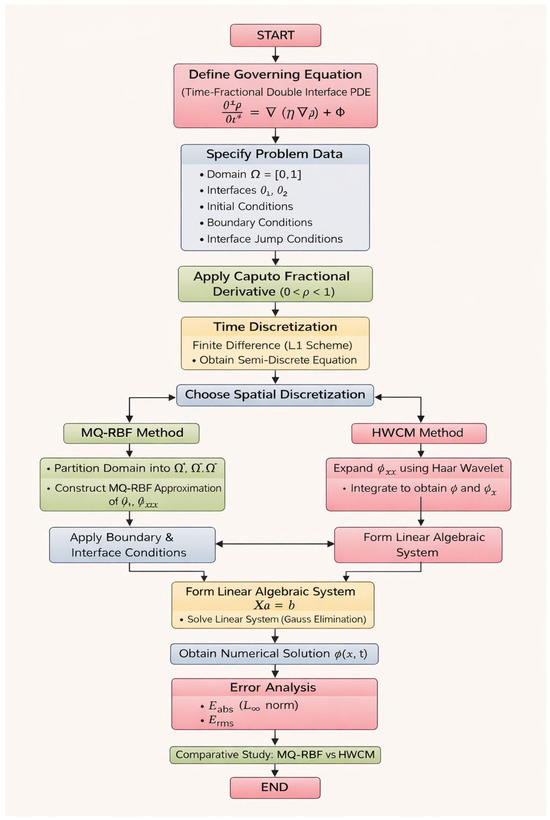
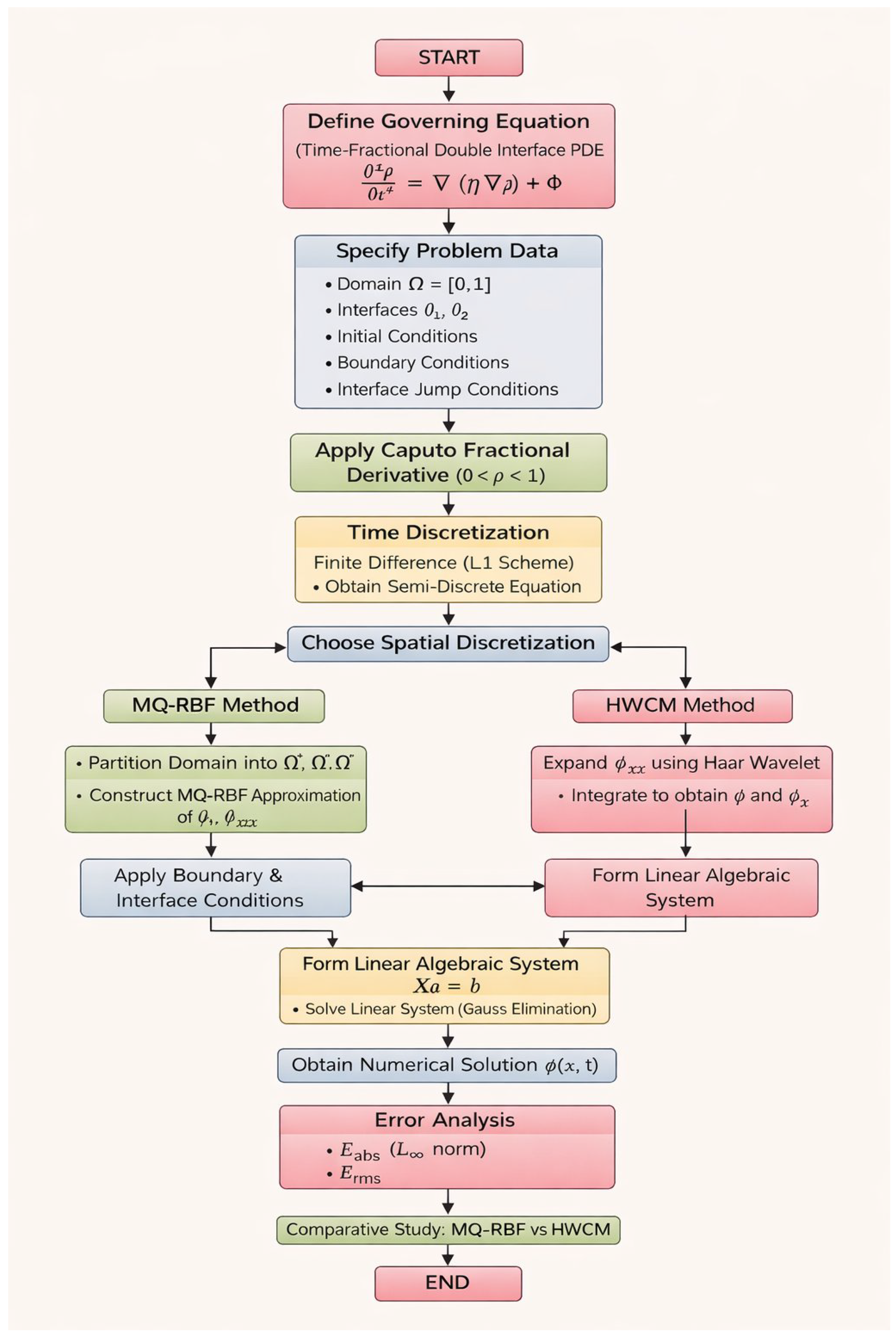
The stability of the proposed MQ-RBF and HWCM methods (Figure 2) is analyzed according to the fundamental definition of stability for numerical schemes, as outlined in LeVeque’s work [63].

Figure 2. Flowchart of the proposed computational framework for solving the time-fractional double interface problem using MQ-RBF and HWCM methods.

Definition 2.

For the numerical solution of the interface problem, the system $\mathbf{X}a=b$ is considered stable when the matrix $\mathbf{X}$ admits a bounded inverse, ensuring that small changes in b do not cause unbounded variations in a.

$$\parallel {\mathbf{X}}^{-1}\parallel \le l_0,$$

where $l_0$ is a constant.

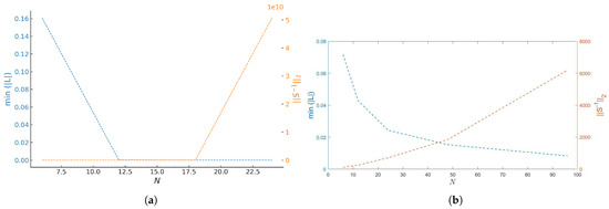
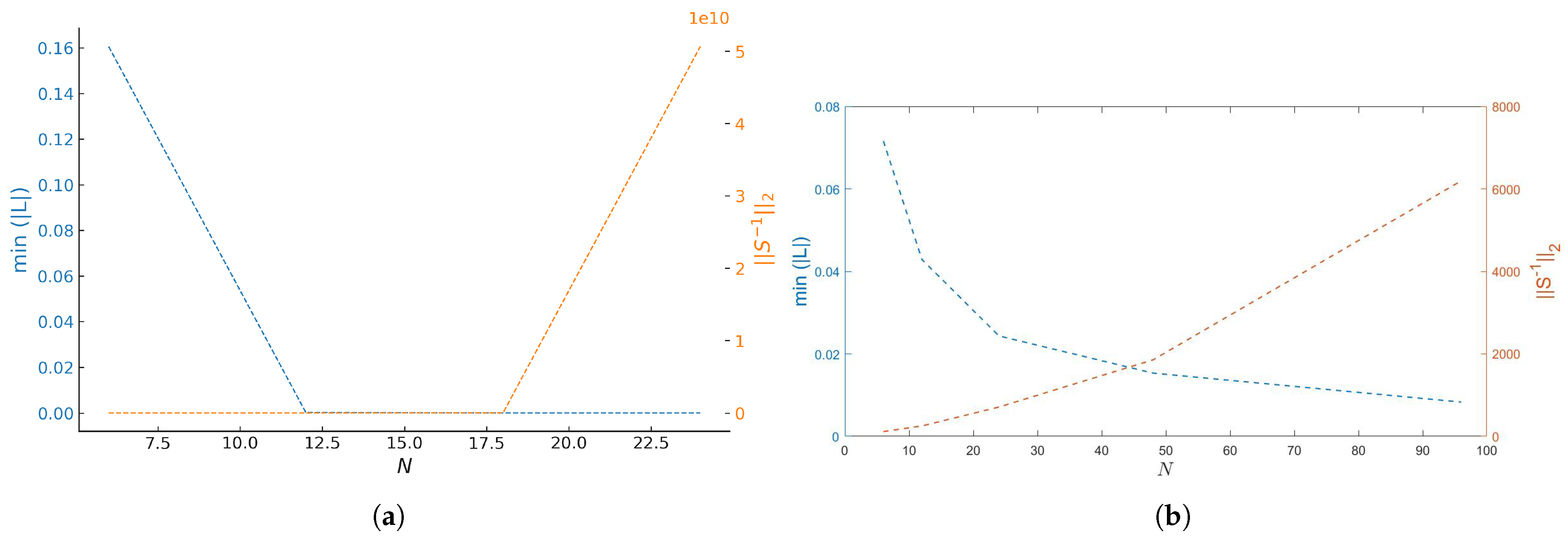
According to Definition 2, the numerical scheme is said to be stable if the inverse of the system matrix X remains bounded, i.e., $\parallel X^{-1}\parallel \le l_0$. In Figure 3, the 2-norm and the spectral radius of $X^{-1}$ are plotted for the proposed methods at $\Delta t=0.5$ and $t=1$. It is clearly observed that both quantities remain bounded for all tested discretization parameters. This bounded behavior confirms that small perturbations in the right-hand side do not lead to unbounded growth in the numerical solution. Hence, the stability condition stated in Definition 2 is satisfied, and the proposed numerical schemes are stable.

Figure 3. The magnitudes of the 2-norm together with the spectral radius of ${\mathbf{X}}^{-1}$ for the proposed approaches at $\Delta t=0.5$, with $t=1$, are presented for (a) Example 1 and (b) Example 3, respectively.

7. Numerical Validation

To evaluate the performance of both the MQ-RBF and HWCM methods, numerical solutions for the time-fractional interface problems are computed, and their accuracy is quantified using the following error norms:

$$\begin{array}{ccc}\hfill E_{abs}& =& \left|\right|{\phi }^{true}-{\phi }^{approx}{\left|\right|}_{\infty }\approx max(|{\phi }_j^{true}-{\phi }_j^{approx}|),\hfill \end{array}$$

(62)

$$\begin{array}{ccc}\hfill E_{rms}& \approx & \sqrt{\left({\displaystyle \frac{1}{\mathcal{M}}}\sum _{j=1}^{\mathcal{M}}{({\phi }_j^{true}-{\phi }_j^{approx})}^2\right)},\hfill \end{array}$$

(63)

and

$${\mathcal{R}}_c(\mathcal{M})={\displaystyle \frac{log[{\mathrm{E}}_c(\mathcal{M}/2)/{\mathrm{E}}_c(\mathcal{M})]}{log(2)}}.$$

(64)

The errors obtained from both methods are subsequently compared to assess their relative accuracy and efficiency.

Example 1.

In the first example, the linear time-fractional interface problem (1) is considered with ${\eta }^{+}(\mathcal{x})=1,$${\eta }^0(\mathcal{x})=10$ and ${\eta }^{-}(\mathcal{x})=1000$. The exact solutions and associated source functions are given by

$$\phi (\mathcal{x},t)=\left\{\begin{array}{cc}{\phi }_1(\mathcal{x},t)=\mathcal{x}{e}^{-t},\hfill & \mathcal{x}\in {\Omega }^{+},\hfill \\ {\phi }_2(\mathcal{x},t)=e^{-{\mathcal{x}}^2}{e}^{-t},\hfill & \mathcal{x}\in {\Omega }^0,\hfill \\ {\phi }_3(\mathcal{x},t)={\mathcal{x}}^3{e}^{-t},\hfill & \mathcal{x}\in {\Omega }^{-}.\hfill \end{array}\right.$$

(65)

and

$$f(\mathcal{x},t)=\left\{\begin{array}{cc}{f}_1(\mathcal{x},t)=-t^{1-\rho }{\mathcal{M}}_{1,2-\rho }(-t)\mathcal{x},\hfill & \mathcal{x}\in {\Omega }^{+},\hfill \\ f_2(\mathcal{x},t)=-t^{1-\rho }{\mathcal{M}}_{1,2-\rho }(-t)\mathcal{x}{e}^{-{\mathcal{x}}^2}-40{\mathcal{x}}^2{e}^{-{\mathcal{x}}^2}{e}^{-t}+20e^{-{\mathcal{x}}^2}{e}^{-t},\hfill & \mathcal{x}\in {\Omega }^0,\hfill \\ f_3(\mathcal{x},t)=-t^{1-\rho }{\mathcal{M}}_{1,2-\rho }(-t)\mathcal{x}{e}^{-{\mathcal{x}}^2}-6000\mathcal{x}{e}^{-t},\hfill & \mathcal{x}\in {\Omega }^{-},\hfill \end{array}\right.$$

(66)

where ${\mathcal{M}}_{a,b}(·)$ is the Mittag-Leffler function of two parameters defined as

$${\mathcal{M}}_{a,b}(t)=\sum _{k=0}^{\infty }{\displaystyle \frac{t^k}{\Gamma (ak+b)}},\forall t\in \mathbb{C},a,b\in {\mathbb{R}}^{+}$$

and

$${\mathcal{M}}_{1,1}(t)=exp(t),\forall t\in \mathbb{C}.$$

From the exact solution prescribed, the initial, boundary and interface conditions are obtained. This problem is linear in nature, and the results corresponding to both numerical schemes are summarized in Table 1, Table 2 and Table 3. Comparative analysis reveals that HWCM yields better accuracy than the MQ-RBF scheme in different time steps, collocation points, and fractional orders $\rho$. For every value tested of $\rho$, HWCM consistently outperforms MQ-RBF. For example, at $\mathcal{M}=48$, HWCM achieves errors of the order ${10}^{-5}$, while MQ-RBF remains at the order ${10}^{-4}$. Furthermore, an increase in the number of collocation points leads to improved accuracy in both methods, with HWCM demonstrating a more pronounced reduction in error. Although HWCM incurs a slightly higher computational cost, its enhanced precision across varying parameters confirms its efficiency and robustness relative to MQ-RBF. Different shape parameters were tested, and the best accuracy was obtained for $ϵ=1$ (see Table 3). The convergence rate for HWCM has been calculated and Table 4 confirms that the method achieves second-order accuracy. For both HWCM and MQ-RBF, errors decrease as the fractional order $\rho$ increases from $0.6$ to 1, while smaller values of $\rho$ yield relatively larger errors due to stronger memory effects. Since interface problems involve discontinuities and abrupt changes, achieving high precision is challenging; however, HWCM consistently outperforms MQ-RBF in all values of $\rho$, demonstrating greater robustness for such problems.

Table 1. Error and CPU evaluation for different values of $\rho$ and $\mathcal{M}$ across various time steps using the HWCM for Example 1 with $t=1$.

$\mathcal{M}$	$\mathbf{\Delta }\mathit{t}$	$\mathit{\rho }=0.6$			$\mathit{\rho }=0.8$			$\mathit{\rho }=1$
		${\mathit{E}}_{\mathit{abs}}$	${\mathit{E}}_{\mathit{rms}}$	CPU (s)	${\mathit{E}}_{\mathit{abs}}$	${\mathit{E}}_{\mathit{rms}}$	CPU (s)	${\mathit{E}}_{\mathit{abs}}$	${\mathit{E}}_{\mathit{rms}}$	CPU (s)
6	0.5/4	$3.42\times {10}^{-3}$	$2.33\times {10}^{-3}$	0.1874	$3.32\times {10}^{-3}$	$2.28\times {10}^{-3}$	0.1661	$2.96\times {10}^{-3}$	$2.09\times {10}^{-3}$	0.1849
12	0.5/8	$9.39\times {10}^{-4}$	$6.29\times {10}^{-4}$	0.1917	$9.52\times {10}^{-4}$	$6.36\times {10}^{-4}$	0.1864	$7.69\times {10}^{-4}$	$5.44\times {10}^{-4}$	0.1998
24	0.5/12	$2.37\times {10}^{-4}$	$1.59\times {10}^{-4}$	0.3303	$2.89\times {10}^{-4}$	$1.85\times {10}^{-4}$	0.3114	$1.72\times {10}^{-4}$	$1.25\times {10}^{-4}$	0.2841
48	0.5/16	$4.33\times {10}^{-5}$	$2.92\times {10}^{-5}$	0.6240	$1.08\times {10}^{-4}$	$6.52\times {10}^{-5}$	0.6489	$4.21\times {10}^{-5}$	$2.15\times {10}^{-5}$	0.5847

Table 2. Error evaluation for different values of $\rho$ and $\mathcal{M}$ across various time steps using the MQ-RBF for Example 1 with $ϵ=2$ and $t=1$.

$\mathcal{M}$	$\mathbf{\Delta }\mathit{t}$	$\mathit{\rho }=0.6$			$\mathit{\rho }=0.8$			$\mathit{\rho }=1$
		${\mathit{E}}_{\mathit{abs}}$	${\mathit{E}}_{\mathit{rms}}$	CPU (s)	${\mathit{E}}_{\mathit{abs}}$	${\mathit{E}}_{\mathit{rms}}$	CPU (s)	${\mathit{E}}_{\mathit{abs}}$	${\mathit{E}}_{\mathit{rms}}$	CPU (s)
6	0.5/4	$3.44\times {10}^{-2}$	$2.37\times {10}^{-2}$	0.3809	$3.40\times {10}^{-2}$	$2.35\times {10}^{-2}$	0.4148	$3.34\times {10}^{-2}$	$2.32\times {10}^{-2}$	0.3954
12	0.5/8	$6.83\times {10}^{-3}$	$4.58\times {10}^{-3}$	0.3005	$6.24\times {10}^{-3}$	$4.30\times {10}^{-3}$	0.3681	$5.43\times {10}^{-3}$	$3.91\times {10}^{-3}$	0.3279
18	0.5/12	$1.83\times {10}^{-3}$	$1.12\times {10}^{-3}$	0.3253	$1.21\times {10}^{-3}$	$8.08\times {10}^{-4}$	0.2947	$8.61\times {10}^{-4}$	$4.48\times {10}^{-4}$	0.3063
24	0.5/16	$9.54\times {10}^{-4}$	$5.31\times {10}^{-4}$	0.3338	$3.24\times {10}^{-4}$	$1.92\times {10}^{-4}$	0.3174	$5.34\times {10}^{-4}$	$3.02\times {10}^{-4}$	0.3297

Table 3. Error evaluation for different values of $\rho$ and $\mathcal{M}$ across various time steps using the MQ-RBF for Example 1 with $ϵ=1$ and $t=1$.

$\mathcal{M}$	$\mathbf{\Delta }\mathit{t}$	$\mathit{\rho }=0.6$			$\mathit{\rho }=0.8$			$\mathit{\rho }=1$
		${\mathit{E}}_{\mathit{abs}}$	${\mathit{E}}_{\mathit{rms}}$	CPU (s)	${\mathit{E}}_{\mathit{abs}}$	${\mathit{E}}_{\mathit{rms}}$	CPU (s)	${\mathit{E}}_{\mathit{abs}}$	${\mathit{E}}_{\mathit{rms}}$	CPU (s)
6	0.5/4	$1.71\times {10}^{-2}$	$1.20\times {10}^{-2}$	0.3589	$1.66\times {10}^{-2}$	$1.18\times {10}^{-2}$	0.3902	$1.59\times {10}^{-2}$	$1.14\times {10}^{-2}$	0.3816
12	0.5/8	$1.94\times {10}^{-3}$	$1.23\times {10}^{-3}$	0.3455	$1.32\times {10}^{-3}$	$9.17\times {10}^{-4}$	0.3804	$1.04\times {10}^{-3}$	$5.65\times {10}^{-4}$	0.3179
18	0.5/12	$8.37\times {10}^{-4}$	$4.62\times {10}^{-4}$	0.3289	$2.11\times {10}^{-4}$	$1.18\times {10}^{-4}$	0.3204	$6.48\times {10}^{-4}$	$3.64\times {10}^{-4}$	0.2715

Table 4. Rate of convergence based on the absolute error $E_{abs}$ for different values of $\rho$ using the HWCM for Example 1 with $t=1$.

$\mathcal{M}$	Rate of Convergence
	$\mathit{\rho }=\mathbf{0.6}$	$\mathit{\rho }=\mathbf{0.8}$	$\mathit{\rho }=\mathbf{1}$
$6\to 12$	1.86	1.80	1.95
$12\to 24$	1.99	1.72	2.16
$24\to 48$	2.45	1.42	2.03

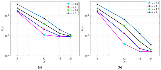
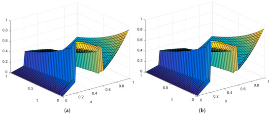
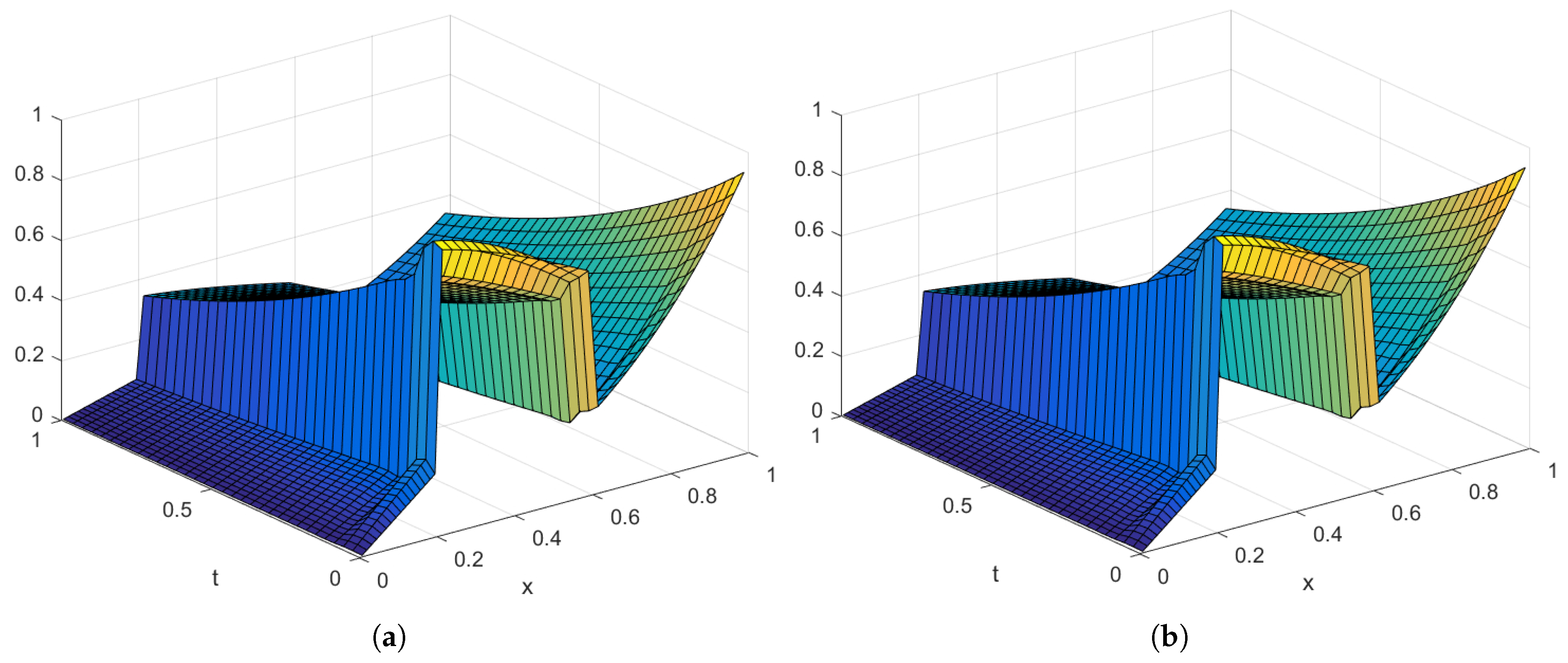
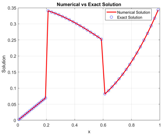
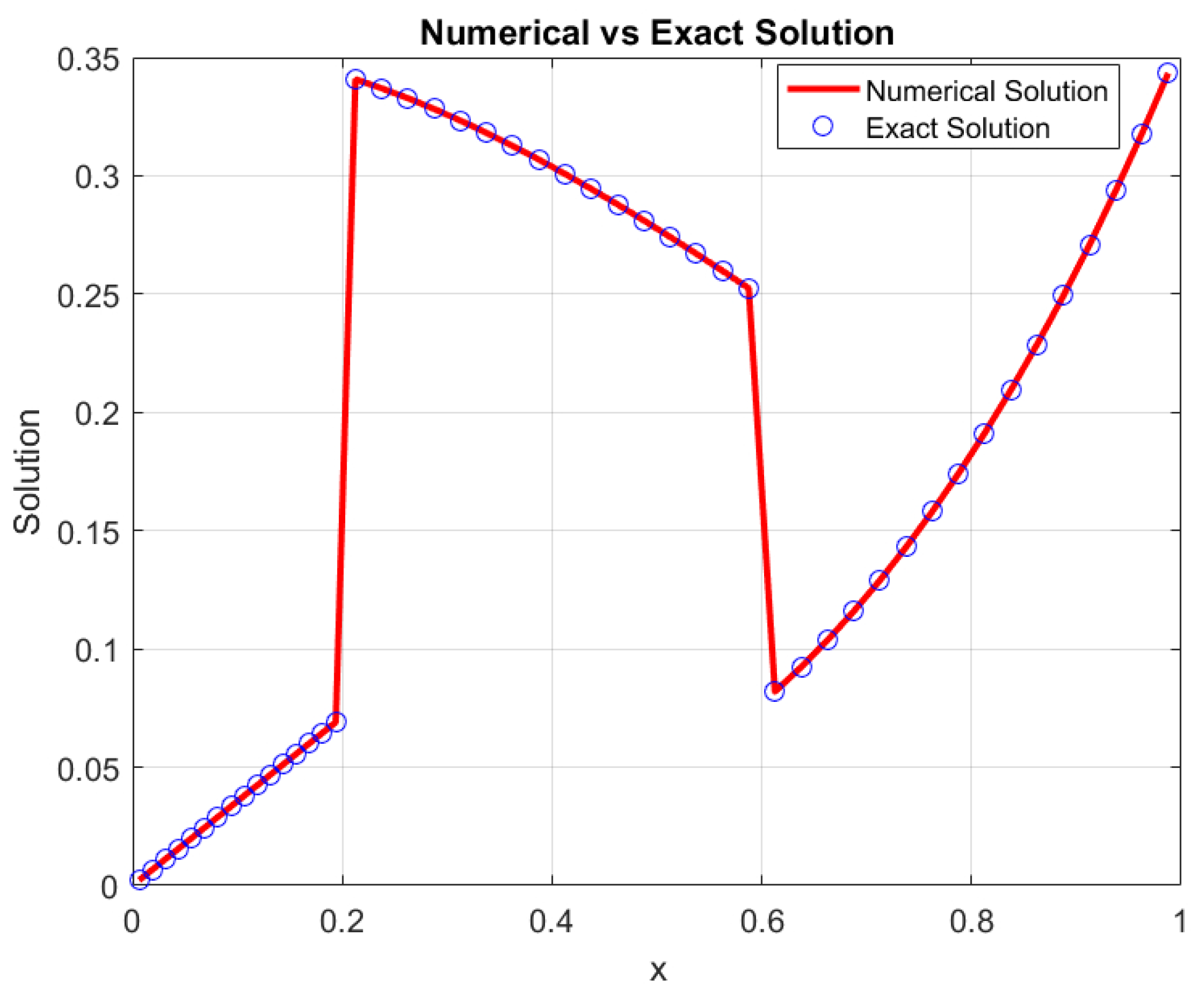
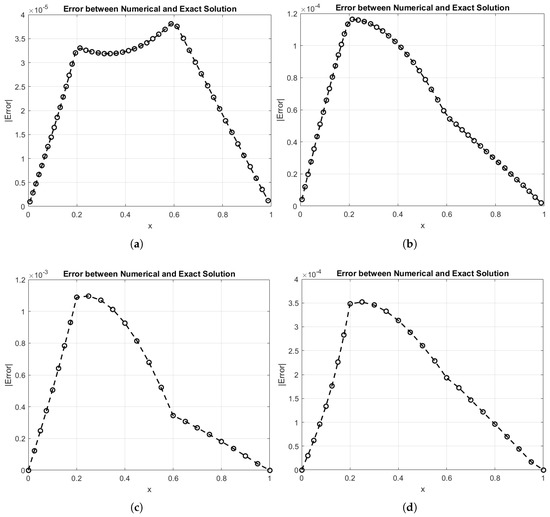
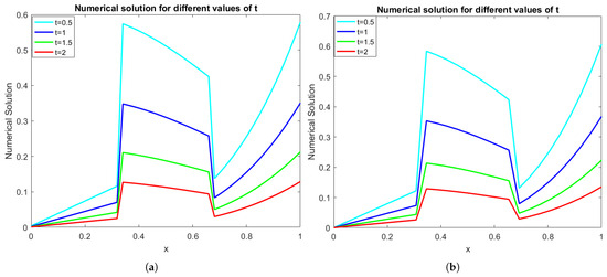
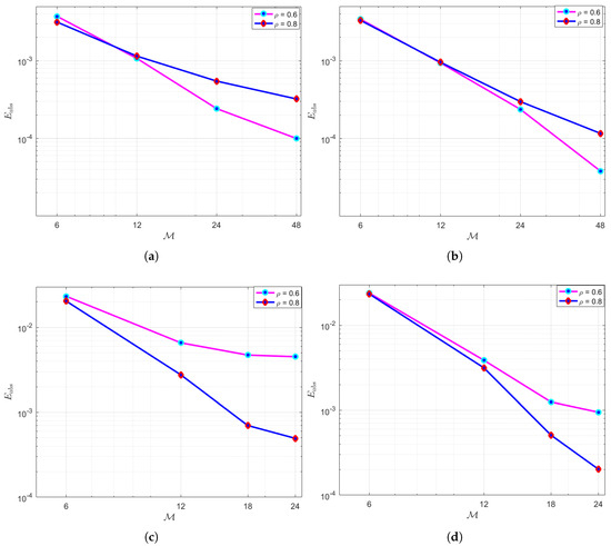
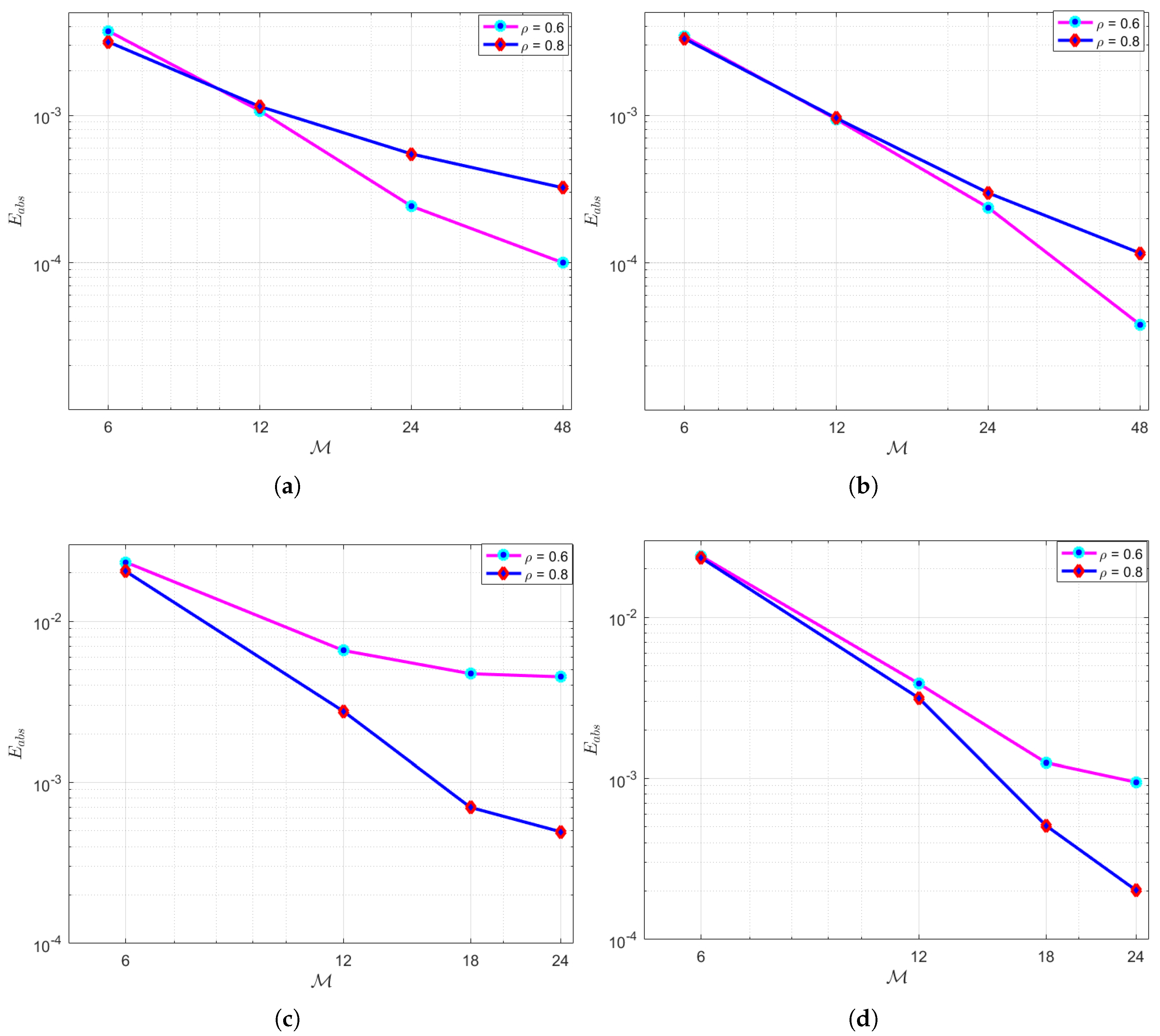
Figure 4, Figure 5, Figure 6, Figure 7 and Figure 8 present the numerical performance of the proposed methods for Example 1. From Figure 4, it is clear that HWCM achieves lower absolute errors than MQ-RBF on different fractional orders $\rho$. Figure 5 shows whether the error varies with $\mathcal{M}$ as $ϵ$ varies. The graphs show how the value of $ϵ$ significantly affects the precision of the method. In general, more $ϵ$ values result in more errors, while lower values result in better convergence and fewer errors. This highlights how important it is to select the appropriate shape parameter in order to receive accurate numerical results. Figure 6 and Figure 7 show that the HWCM solutions closely follow the exact ones, with only slight deviations near the interfaces. Finally, Figure 8 illustrates that HWCM captures the behavior of the interface more accurately, keeping the errors localized, while MQ-RBF produces more spread out errors throughout the domain. Figure 9 shows that for different values of t, both MQ-RBF and HWCM yield stable and closely agreeing results.

Figure 4. Comparison of $E_{abs}$ for different values of $\rho$ using (a) HWCM and (b) MQ-RBF at $t=1$.

Figure 5. Comparison of $E_{\mathrm{abs}}$ versus collocation points $\mathcal{M}$ for different shape parameters $ϵ$ at fractional orders (a) $\rho =0.6$ and (b) $\rho =0.8$.

Figure 6. (a) Exact versus (b) approximate solution for Example 1 is presented for distinct values of x and t with $\rho =0.6$.

Figure 7. True vs. computed solutions for Example 1 using HWCM.

Figure 8. Error between exact and numerical solutions using both methods at different values of $\rho .$ (a) Error between exact and numerical solutions using HWCM at $\rho =0.6$ for Example 1. (b) Error between exact and numerical solutions using HWCM at $\rho =0.8$. (c) Error between exact and numerical solutions using MQ-RBFs at $\rho =0.6$. (d) Error between exact and numerical solutions using MQ-RBFs at $\rho =0.8$.

Figure 9. (a) Numerical solution profiles for different values of t using HWCM. (b) Numerical solution profiles for different values of t using MQ-RBF for Example 1 are presented for $\mathcal{M}=24$ $\rho =0.6$.

Example 2.

In the second example, the linear time-fractional interface problem (1) is considered with two different types of constant coefficients. The exact solutions are given by

$$\phi (\mathcal{x},t)=\left\{\begin{array}{cc}{\phi }_1(\mathcal{x},t)=\mathcal{x}{e}^{-t},\hfill & \mathcal{x}\in {\Omega }^{+},\hfill \\ {\phi }_2(\mathcal{x},t)=e^{-{\mathcal{x}}^2}{e}^{-t},\hfill & \mathcal{x}\in {\Omega }^0,\hfill \\ {\phi }_3(\mathcal{x},t)={\mathcal{x}}^3{e}^{-t},\hfill & \mathcal{x}\in {\Omega }^{-}.\hfill \end{array}\right.$$

(67)

The source function is constructed using the exact solution by substituting it into the governing Equation (1), with coefficients taken as ${\eta }^{+}(\mathcal{x})=1,$${\eta }^0(\mathcal{x})=2$ and ${\eta }^{-}(\mathcal{x})=3$

$$f(\mathcal{x},t)=\left\{\begin{array}{cc}{f}_1(\mathcal{x},t)=-t^{1-\rho }{\mathcal{M}}_{1,2-\rho }(-t)\mathcal{x},\hfill & \mathcal{x}\in {\Omega }^{+},\hfill \\ f_2(\mathcal{x},t)=-t^{1-\rho }{\mathcal{M}}_{1,2-\rho }(-t)\mathcal{x}{e}^{-{\mathcal{x}}^2}-8{\mathcal{x}}^2{e}^{-{\mathcal{x}}^2}{e}^{-t}+4e^{-{\mathcal{x}}^2}{e}^{-t},\hfill & \mathcal{x}\in {\Omega }^0,\hfill \\ f_3(\mathcal{x},t)=-t^{1-\rho }{\mathcal{M}}_{1,2-\rho }(-t)\mathcal{x}{e}^{-{\mathcal{x}}^2}-18\mathcal{x}{e}^{-t},\hfill & \mathcal{x}\in {\Omega }^{-},\hfill \end{array}\right.$$

(68)

Now, taking the other coefficients ${\eta }^{+}(\mathcal{x})=1,$${\eta }^0(\mathcal{x})=10$ and ${\eta }^{-}(\mathcal{x})=100$, we determine the corresponding source function.

$$f(\mathcal{x},t)=\left\{\begin{array}{cc}{f}_1(\mathcal{x},t)=-t^{1-\rho }{\mathcal{M}}_{1,2-\rho }(-t)\mathcal{x},\hfill & \mathcal{x}\in {\Omega }^{+},\hfill \\ f_2(\mathcal{x},t)=-t^{1-\rho }{\mathcal{M}}_{1,2-\rho }(-t)\mathcal{x}{e}^{-{\mathcal{x}}^2}-40{\mathcal{x}}^2{e}^{-{\mathcal{x}}^2}{e}^{-t}+20e^{-{\mathcal{x}}^2}{e}^{-t},\hfill & \mathcal{x}\in {\Omega }^0,\hfill \\ f_3(\mathcal{x},t)=-t^{1-\rho }{\mathcal{M}}_{1,2-\rho }(-t)\mathcal{x}{e}^{-{\mathcal{x}}^2}-300\mathcal{x}{e}^{-t},\hfill & \mathcal{x}\in {\Omega }^{-},\hfill \end{array}\right.$$

(69)

where ${\mathcal{M}}_{a,b}(·)$ is the Mittag-Leffler function of two parameters defined as

$${\mathcal{M}}_{a,b}(t)=\sum _{k=0}^{\infty }{\displaystyle \frac{t^k}{\Gamma (ak+b)}},\forall t\in \mathbb{C},a,b\in {\mathbb{R}}^{+}$$

and

$${\mathcal{M}}_{1,1}(t)=exp(t),\forall t\in \mathbb{C}.$$

The initial, boundary, and interface conditions are taken from the exact solution, which allows a fair and direct comparison between the two methods. Since the initial, boundary, and interface conditions are extracted from the exact solution, a direct and equitable comparison of the two approaches is made possible. The detailed numerical results of both HWCM and MQ-RBF schemes are reported in Table 5, Table 6, Table 7, Table 8 and Table 9. From the numerical results, it is clear that HWCM provides smaller absolute and root mean square errors than the MQ-RBF scheme. For example, when $M=48$, the HWCM errors reduce to approximately ${10}^{-5}$ and ${10}^{-4}$, while the MQ-RBF errors remain around ${10}^{-3}$ and ${10}^{-4}$. This shows that HWCM achieves better accuracy by one to two orders of magnitude. When the coefficients are more strongly varying, such as $(1,10,100)$, the errors increase for both methods, but HWCM still performs better. Another important point is that HWCM maintains good accuracy even at the lower fractional order $\rho =0.6$, sometimes even better than at larger $\rho$. This indicates that HWCM is more stable against the strong memory effects that appear for smaller $\rho$. By contrast, MQ-RBF improves only when $\rho$ gets closer to 1, and even then, it does not capture the sharp interface transitions as well as HWCM.

Table 5. HWCM errors and rate of convergence for Problem 2 with coefficient set $({\eta }^{+},{\eta }^0,{\eta }^{-})=(1,2,3)$.

$\mathcal{M}$	$\mathbf{\Delta }\mathit{t}$	$\mathit{\rho }=0.6$					$\mathit{\rho }=0.8$
		${\mathit{E}}_{\mathbf{abs}}$	${\mathit{E}}_{\mathbf{rms}}$	CPU (s)	CPU Time Ratio	Rate of Convergence	${\mathit{E}}_{\mathbf{abs}}$	${\mathit{E}}_{\mathbf{rms}}$	CPU (s)	CPU Time Ratio	Rate of Convergence
6	0.5/4	3.7367 × 10−3	2.6828 × 10−3	0.0779	–	–	3.1533 × 10−3	2.2672 × 10−3	0.1943	–	–
12	0.5/8	1.0735 × 10−3	7.4921 × 10−4	0.1662	2.13	1.80	1.1481 × 10−3	7.9950 × 10−4	0.1955	1.01	1.46
24	0.5/12	2.4188 × 10−4	1.6855 × 10−4	0.3357	2.02	2.15	5.4700 × 10−4	3.7330 × 10−4	0.3409	1.74	1.07
48	0.5/16	9.9833 × 10−5	6.5842 × 10−5	0.6405	1.91	1.28	3.2219 × 10−4	2.1740 × 10−4	0.6384	1.87	0.76

Table 6. HWCM errors and rate of convergence for Problem 2 with coefficient set $({\eta }^{+},{\eta }^0,{\eta }^{-})=(1,10,100)$.

$\mathcal{M}$	$\mathbf{\Delta }\mathit{t}$	$\mathit{\rho }=0.6$					$\mathit{\rho }=0.8$
		${\mathit{E}}_{\mathbf{abs}}$	${\mathit{E}}_{\mathbf{rms}}$	CPU (s)	CPU Time Ratio	Rate of Convergence	${\mathit{E}}_{\mathbf{abs}}$	${\mathit{E}}_{\mathbf{rms}}$	CPU (s)	CPU Time Ratio	Rate of Convergence
6	0.5/4	$3.4146\times {10}^{-3}$	$2.3314\times {10}^{-3}$	0.1706	–	–	$3.3014\times {10}^{-3}$	$2.2674\times {10}^{-3}$	0.0447	–	–
12	0.5/8	$9.3877\times {10}^{-4}$	$6.2946\times {10}^{-4}$	0.1764	1.03	1.86	$9.5508\times {10}^{-4}$	$6.3862\times {10}^{-4}$	0.0379	0.85	1.79
24	0.5/12	$2.3677\times {10}^{-4}$	$1.5823\times {10}^{-4}$	0.3255	1.85	1.99	$2.9756\times {10}^{-4}$	$1.9204\times {10}^{-4}$	0.0871	2.30	1.68
48	0.5/16	$3.8120\times {10}^{-5}$	$2.5579\times {10}^{-5}$	0.6400	1.97	2.64	$1.1634\times {10}^{-4}$	$7.1766\times {10}^{-5}$	0.1110	1.27	1.36

Table 7. Error evaluation and CPU time for different values of $\rho$ and $\mathcal{M}$ across various time steps using the HWCM for Problem (2) with $t=1$.

$\mathcal{M}$	$\mathbf{\Delta }\mathit{t}$	$\mathit{\rho }=0.2$			$\mathit{\rho }=0.5$			$\mathit{\rho }=0.8$			$\mathit{\rho }=1$
		${\mathit{E}}_{\mathit{abs}}$	${\mathit{E}}_{\mathit{rms}}$	CPU	${\mathit{E}}_{\mathit{abs}}$	${\mathit{E}}_{\mathit{rms}}$	CPU	${\mathit{E}}_{\mathit{abs}}$	${\mathit{E}}_{\mathit{rms}}$	CPU	${\mathit{E}}_{\mathit{abs}}$	${\mathit{E}}_{\mathit{rms}}$	CPU
6	0.5	$1.5969\times {10}^{-2}$	$1.1140\times {10}^{-2}$	0.026	$7.6396\times {10}^{-3}$	$5.3078\times {10}^{-3}$	0.033	$2.6069\times {10}^{-3}$	$1.7833\times {10}^{-3}$	0.113	$2.0552\times {10}^{-3}$	$1.3960\times {10}^{-3}$	0.111
12	0.5/2	$4.6774\times {10}^{-3}$	$3.1936\times {10}^{-3}$	0.021	$8.1969\times {10}^{-3}$	$5.5711\times {10}^{-3}$	0.020	$4.9136\times {10}^{-3}$	$3.3457\times {10}^{-3}$	0.071	$1.4939\times {10}^{-3}$	$9.9262\times {10}^{-4}$	0.068
24	0.5/4	$8.3552\times {10}^{-4}$	$5.5705\times {10}^{-4}$	0.038	$2.1584\times {10}^{-3}$	$1.4562\times {10}^{-3}$	0.034	$1.8385\times {10}^{-3}$	$1.2421\times {10}^{-3}$	0.129	$8.8529\times {10}^{-4}$	$5.9039\times {10}^{-4}$	0.108

Table 8. MQ-RBF errors for Problem 2 with coefficient set $({\eta }^{+},{\eta }^0,{\eta }^{-})=(1,2,3)$ and $ϵ=1.5$.

$\mathcal{M}$	$\mathbf{\Delta }\mathit{t}$	$\mathit{\rho }=0.2$				$\mathit{\rho }=0.6$				$\mathit{\rho }=0.8$
		${\mathit{E}}_{\mathbf{abs}}$	${\mathit{E}}_{\mathbf{rms}}$	CPU (s)	CPU Time Ratio	${\mathit{E}}_{\mathbf{abs}}$	${\mathit{E}}_{\mathbf{rms}}$	CPU (s)	CPU Time Ratio	${\mathit{E}}_{\mathbf{abs}}$	${\mathit{E}}_{\mathbf{rms}}$	CPU (s)	CPU Time Ratio
6	0.5/4	$2.5725\times {10}^{-2}$	$1.8058\times {10}^{-2}$	0.2685	–	$2.3225\times {10}^{-2}$	$1.6047\times {10}^{-2}$	0.3749	–	$2.0384\times {10}^{-2}$	$1.3762\times {10}^{-2}$	0.3569	–
12	0.5/8	$1.0301\times {10}^{-2}$	$6.9890\times {10}^{-3}$	0.2606	0.97	$6.5764\times {10}^{-3}$	$4.5265\times {10}^{-3}$	0.3461	0.92	$2.7600\times {10}^{-3}$	$1.8985\times {10}^{-3}$	0.3486	0.98
18	0.5/12	$8.5031\times {10}^{-3}$	$5.6529\times {10}^{-3}$	0.3505	1.35	$4.7150\times {10}^{-3}$	$3.1377\times {10}^{-3}$	0.2882	0.83	$6.9996\times {10}^{-4}$	$4.6524\times {10}^{-4}$	0.2856	0.82
24	0.5/16	$8.3082\times {10}^{-3}$	$5.5048\times {10}^{-3}$	0.0613	0.18	$4.5102\times {10}^{-3}$	$2.9828\times {10}^{-3}$	0.2979	1.03	$4.9392\times {10}^{-4}$	$3.0508\times {10}^{-4}$	0.2845	1.00

Table 9. MQ-RBF errors for Problem 2 with coefficient set $({\eta }^{+},{\eta }^0,{\eta }^{-})=(1,10,100)$ and $ϵ=1.5$.

$\mathcal{M}$	$\mathbf{\Delta }\mathit{t}$	$\mathit{\rho }=0.6$				$\mathit{\rho }=0.8$
		${\mathit{E}}_{\mathbf{abs}}$	${\mathit{E}}_{\mathbf{rms}}$	CPU (s)	CPU Time Ratio	${\mathit{E}}_{\mathbf{abs}}$	${\mathit{E}}_{\mathbf{rms}}$	CPU (s)	CPU Time Ratio
6	0.5/4	$2.3911\times {10}^{-2}$	$1.6873\times {10}^{-2}$	0.3827	–	$2.3357\times {10}^{-2}$	$1.6572\times {10}^{-2}$	0.5971	–
12	0.5/8	$3.8685\times {10}^{-3}$	$2.5991\times {10}^{-3}$	0.2862	0.75	$3.1497\times {10}^{-3}$	$2.2113\times {10}^{-3}$	0.3667	0.61
18	0.5/12	$1.2501\times {10}^{-3}$	$7.4564\times {10}^{-4}$	0.4681	1.64	$5.1028\times {10}^{-4}$	$3.3065\times {10}^{-4}$	0.3439	0.94
24	0.5/16	$9.4775\times {10}^{-4}$	$5.3510\times {10}^{-4}$	0.3002	0.64	$2.0183\times {10}^{-4}$	$1.1172\times {10}^{-4}$	0.3629	1.06

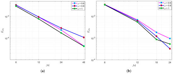
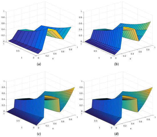
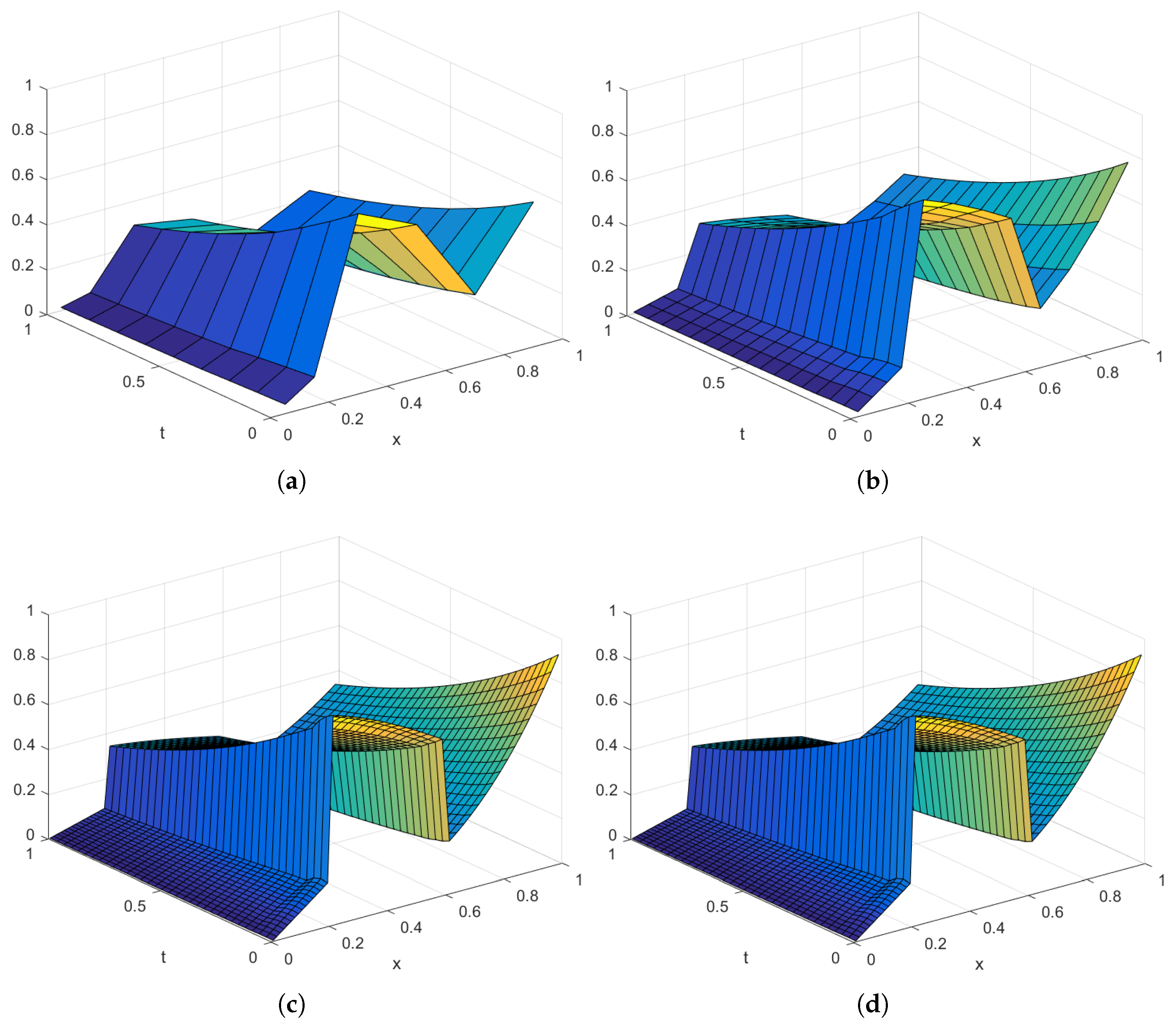
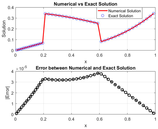
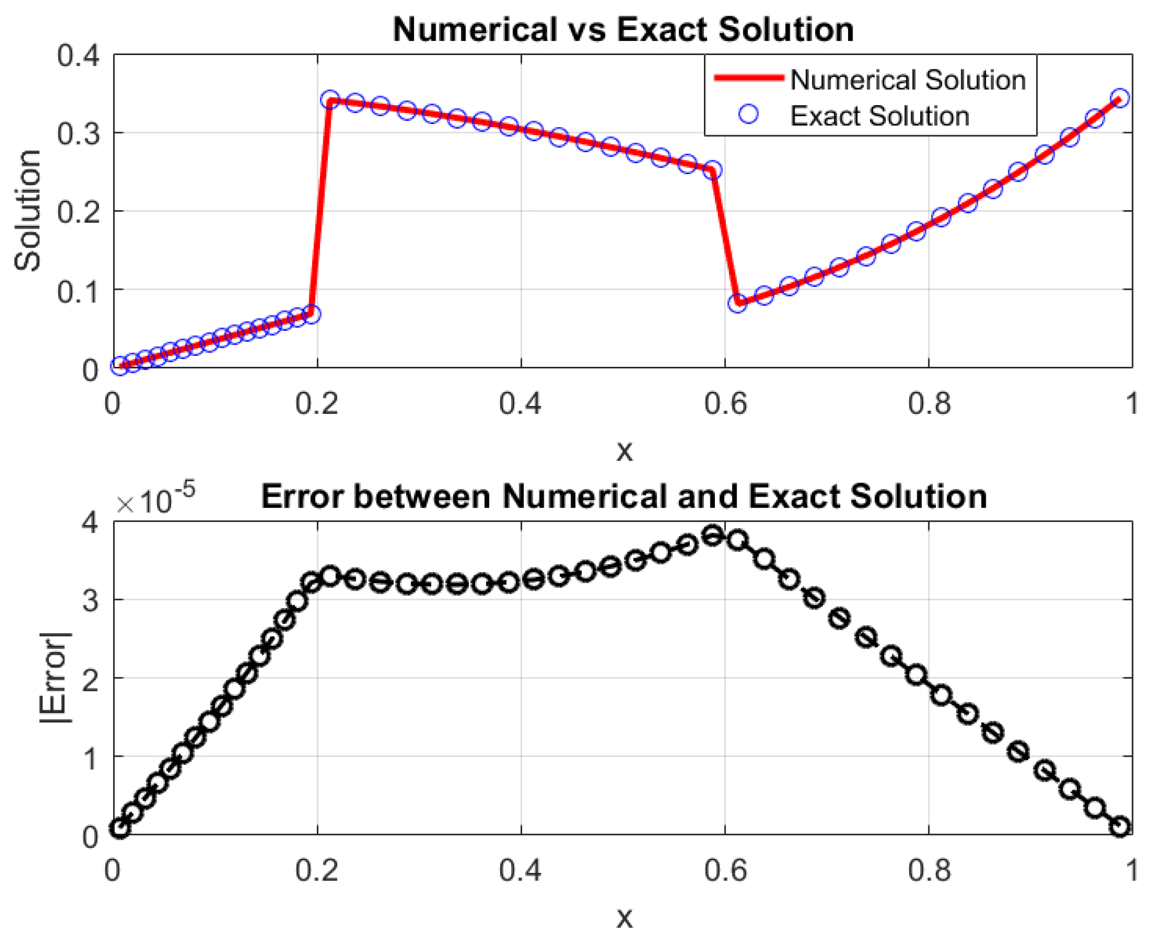
The figures confirm these observations. Figure 10 shows that HWCM consistently produces smaller errors for all values of $\rho$ and for both set of coefficients, the accuracy remaining reliable even at $\rho =0.6$. Figure 11 shows that mesh refinement enhances HWCM performance by reducing errors as the number of collocation points M increases. Figure 12 demonstrates that HWCM closely tracks the exact solution and maintains the absolute error at the interfaces. Overall, the results show that HWCM captures interface behavior more correctly, converges faster with refinement, and is more reliable than MQ-RBF.

Figure 10. Solution profiles for different $\rho$ with varying coefficients using both HWCM and MQ-RBF methods. (a) HWCM solution profiles for different $\rho$ with coefficients $(1,2,3)$ for Example 2. (b) HWCM solution profiles for different $\rho$ with coefficients $(1,10,100)$ for Example 2. (c) MQ-RBFs solution profiles for different $\rho$ with coefficients $(1,2,3)$ for Example 2. (d) MQ-RBFs solution profiles for different $\rho$ with coefficients $(1,10,100)$ for Example 2.

Figure 11. Computed solutions of Problem 2 utilizing HWCM for various numbers of grid points at $t=1$ and $\rho =0.6$. (a) For $\mathcal{N}=6$. (b) For $\mathcal{N}=12$. (c) For $\mathcal{N}=24$. (d) For $\mathcal{N}=48$.

Figure 12. Numerical vs. exact solution (top) and corresponding absolute error (bottom) fractional order $\rho =0.6$ for Example 2 using HWCM.

Example 3.

In the third example, the linear time-fractional interface problem (1) is considered with variable coefficients ${\eta }^{+}(\mathcal{x})=\mathcal{x},$${\eta }^0(\mathcal{x})=2\mathcal{x}$ and ${\eta }^{-}(\mathcal{x})=\mathcal{x}/3$. The exact solutions and associated source functions are given by

$$\phi (\mathcal{x},t)=\left\{\begin{array}{cc}{\phi }_1(\mathcal{x},t)=\mathcal{x}{e}^{-t},\hfill & \mathcal{x}\in {\Omega }^{+},\hfill \\ {\phi }_2(\mathcal{x},t)=e^{-{\mathcal{x}}^2}{e}^{-t},\hfill & \mathcal{x}\in {\Omega }^0,\hfill \\ {\phi }_3(\mathcal{x},t)={\mathcal{x}}^3{e}^{-t},\hfill & \mathcal{x}\in {\Omega }^{-}.\hfill \end{array}\right.$$

(70)

and

$$f(\mathcal{x},t)=\left\{\begin{array}{cc}{f}_1(\mathcal{x},t)=-t^{1-\rho }{\mathcal{M}}_{1,2-\rho }(-t)\mathcal{x}-e^{-t},\hfill & \mathcal{x}\in {\Omega }^{+},\hfill \\ f_2(\mathcal{x},t)=-t^{1-\rho }{\mathcal{M}}_{1,2-\rho }(-t)\mathcal{x}{e}^{-{\mathcal{x}}^2}-4{\mathcal{x}}^3{e}^{-{\mathcal{x}}^2}{e}^{-t}+4\mathcal{x}{e}^{-{\mathcal{x}}^2}{e}^{-t},\hfill & \mathcal{x}\in {\Omega }^0,\hfill \\ f_3(\mathcal{x},t)=-t^{1-\rho }{\mathcal{M}}_{1,2-\rho }(-t)\mathcal{x}{e}^{-{\mathcal{x}}^2}-3{\mathcal{x}}^2{e}^{-t},\hfill & \mathcal{x}\in {\Omega }^{-},\hfill \end{array}\right.$$

(71)

where ${\mathcal{M}}_{a,b}(·)$ is the Mittag-Leffler function of two parameters defined as

$${\mathcal{M}}_{a,b}(t)=\sum _{k=0}^{\infty }{\displaystyle \frac{t^k}{\Gamma (ak+b)}},\forall t\in \mathbb{C},a,b\in {\mathbb{R}}^{+}$$

and

$${\mathcal{M}}_{1,1}(t)=exp(t),\forall t\in \mathbb{C}.$$

From the prescribed exact solution, the initial, boundary, and interface conditions are obtained. In Example 3, we deal with a problem involving variable coefficients in order to test the reliability of the proposed HWCM scheme. The numerical errors reported in Table 10 clearly indicate that the method maintains stable convergence for different fractional orders ρ. When the density of collocation points M is increased, both the $E_{abs}$ and the $E_{rms}$ decrease noticeably, reflecting the effectiveness of the scheme. It is also observed that larger values of ρ lead to higher accuracy, whereas for smaller values of ρ, the errors remain relatively higher, which can be attributed to the stronger memory effect.

Table 10. Error evaluation for different values of $\rho$ and $\mathcal{M}$ across various time steps using the HWCM for Problem 3 with $t=1$.

$\mathcal{M}$	$\mathbf{\Delta }\mathit{t}$	$\mathit{\rho }=0.6$		$\mathit{\rho }=0.8$		$\mathit{\rho }=0.95$
		${\mathit{E}}_{\mathit{abs}}$	${\mathit{E}}_{\mathit{rms}}$	${\mathit{E}}_{\mathit{abs}}$	${\mathit{E}}_{\mathit{rms}}$	${\mathit{E}}_{\mathit{abs}}$	${\mathit{E}}_{\mathit{rms}}$
6	0.5/6	$2.5128\times {10}^{-2}$	$1.9039\times {10}^{-2}$	$8.9874\times {10}^{-3}$	$5.8694\times {10}^{-3}$	$6.4479\times {10}^{-3}$	$4.1065\times {10}^{-3}$
12	0.5/12	$8.0832\times {10}^{-3}$	$6.0382\times {10}^{-3}$	$5.8309\times {10}^{-3}$	$4.0951\times {10}^{-3}$	$2.5583\times {10}^{-3}$	$1.4140\times {10}^{-3}$
24	0.5/24	$2.3111\times {10}^{-3}$	$1.7422\times {10}^{-3}$	$3.0889\times {10}^{-3}$	$2.2823\times {10}^{-3}$	$9.3997\times {10}^{-4}$	$4.8777\times {10}^{-4}$
48	0.5/48	$1.2399\times {10}^{-3}$	$9.5322\times {10}^{-4}$	$9.5680\times {10}^{-4}$	$7.1468\times {10}^{-4}$	$3.8456\times {10}^{-4}$	$2.0349\times {10}^{-4}$

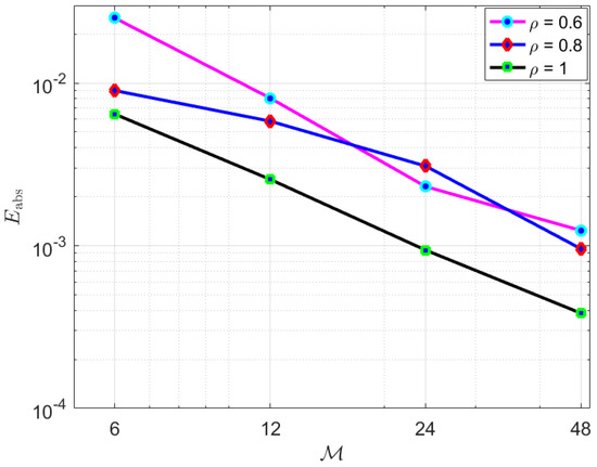
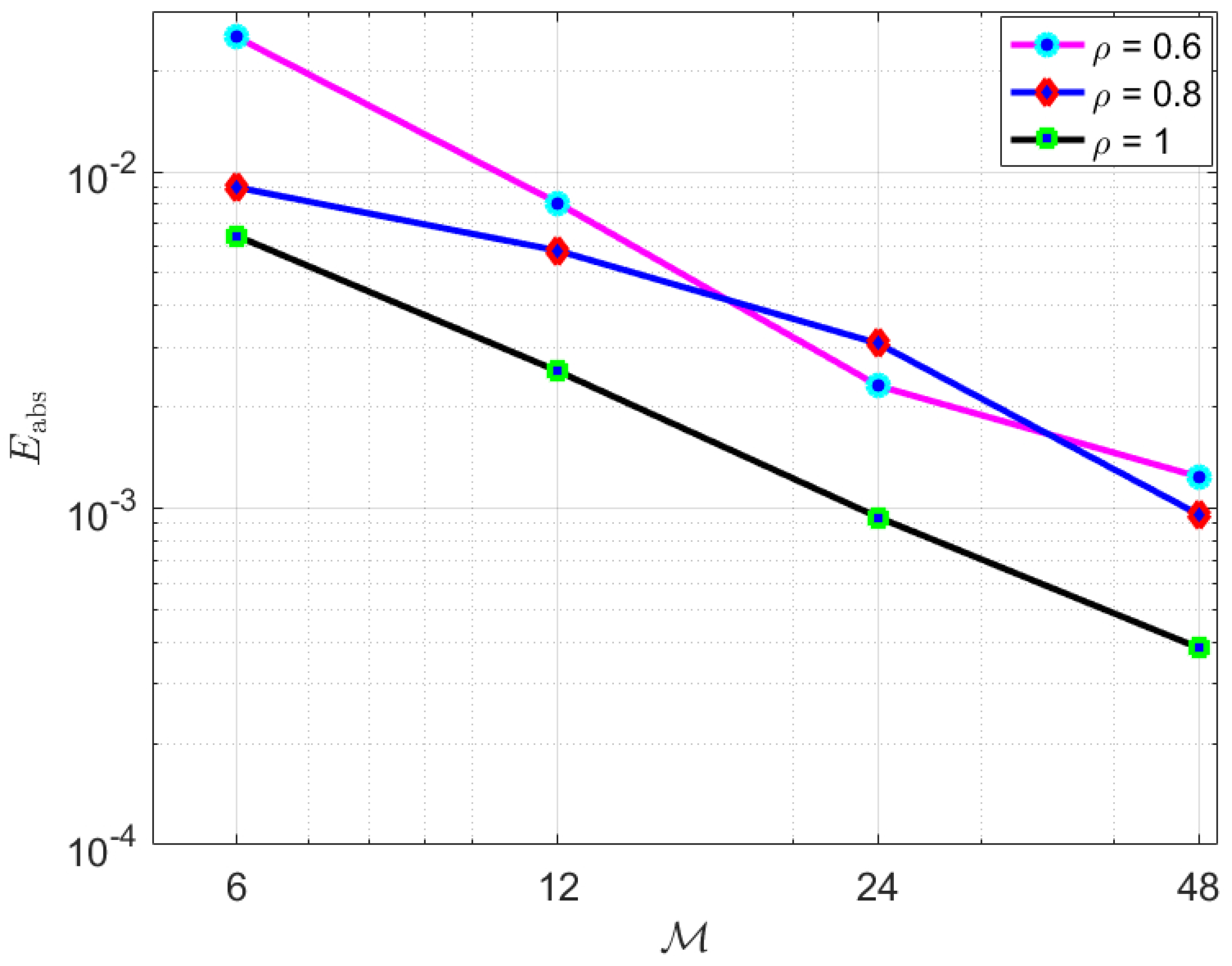
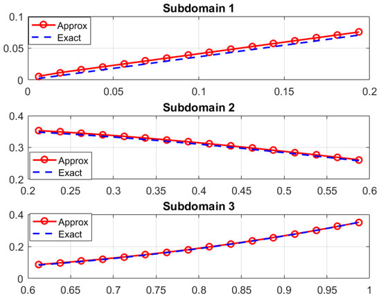
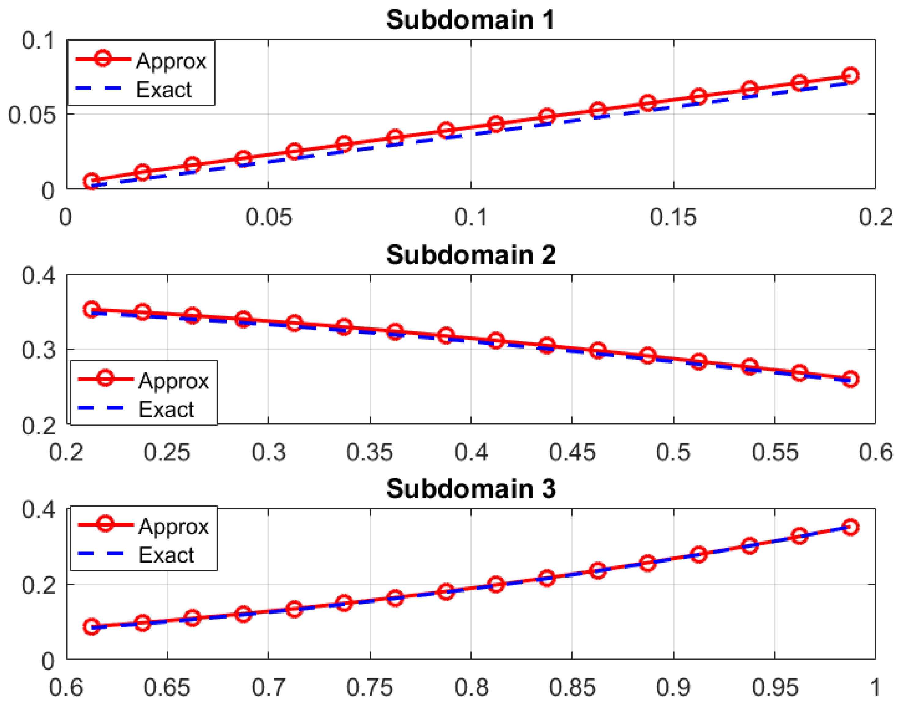
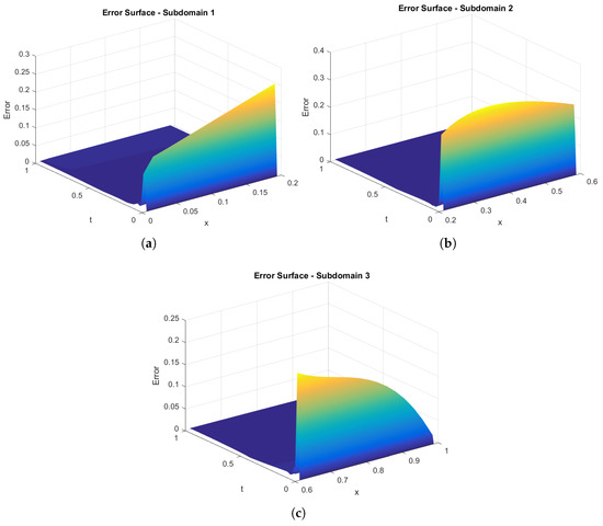
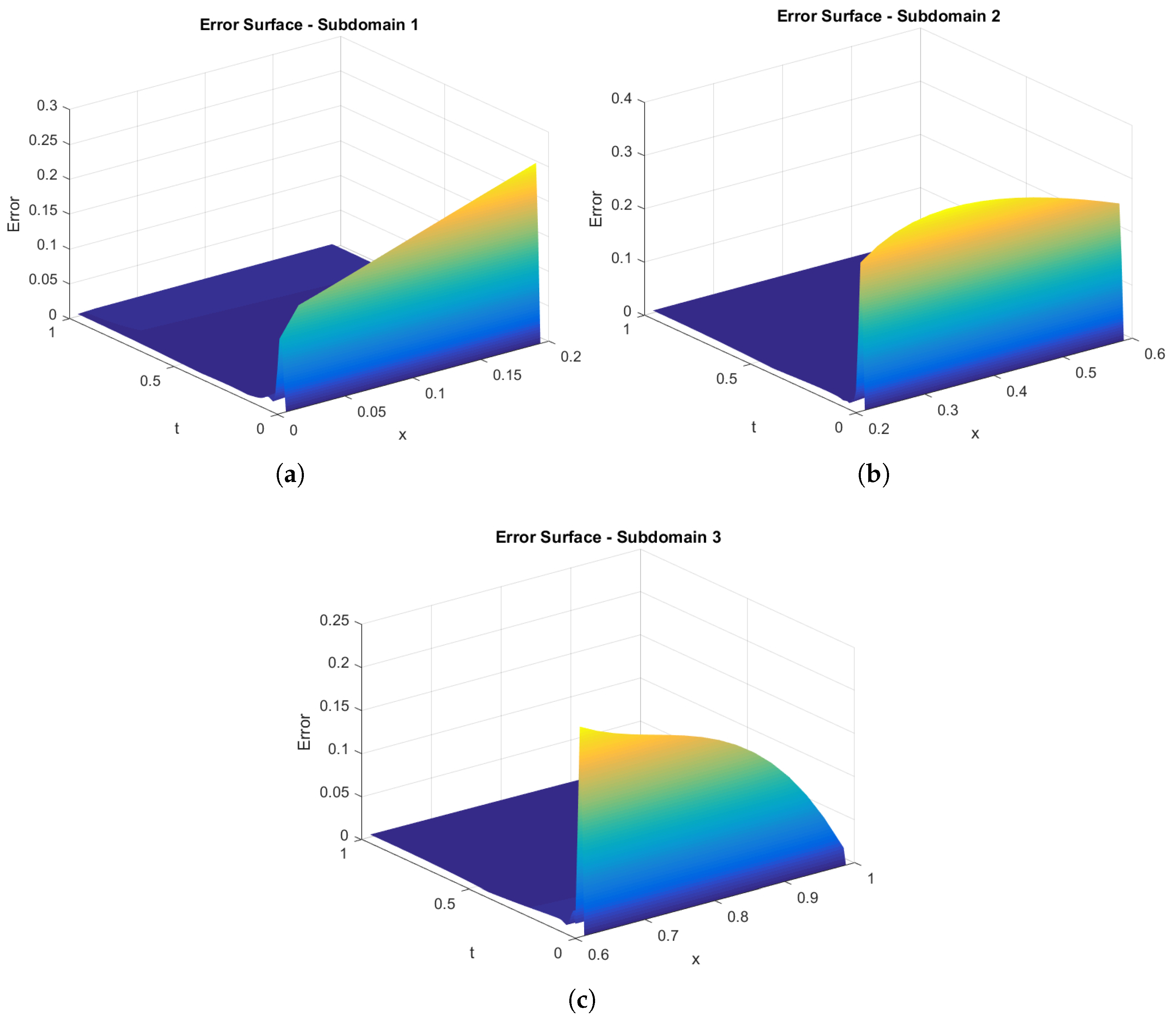
The scheme’s performance can be better understood thanks to the graphical results. Figure 13 illustrates how mesh refinement lowers mistakes; for all values of ρ, a sharp decline in error is observed as M rises. The distribution of absolute errors over the three subdomains $({\Omega }^{+},{\Omega }^0,{\Omega }^{-})$ when $\rho =0.6$ is displayed in Figure 14. The approach maintains localized and well-controlled faults while successfully capturing discontinuities at the interfaces.

Figure 13. Error decay with $\mathcal{M}$ for varying $\rho$ for Example 3.

Figure 14. Subdomain-wise absolute error distribution $({\Omega }^{+},{\Omega }^0,{\Omega }^{-})$ for Example 3 at fractional order $\rho =0.6$, illustrating the accuracy of the proposed scheme in capturing interface behavior.

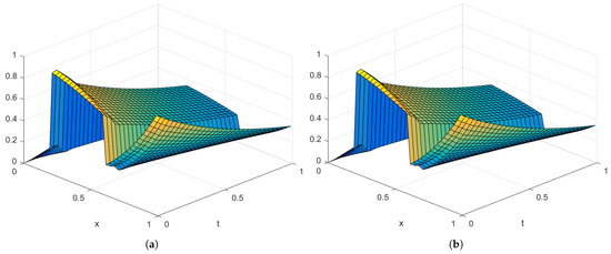
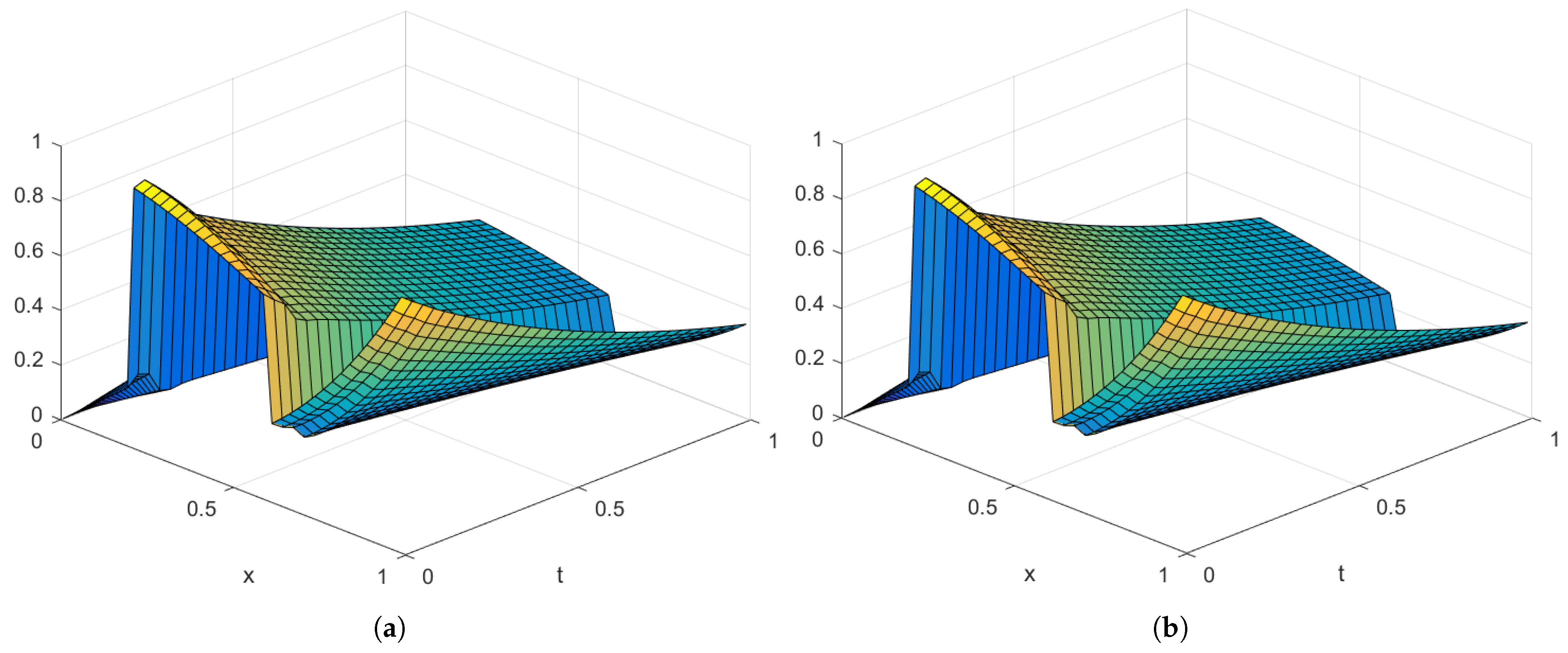
The capacity of the approach to precisely resolve the interface phenomena is confirmed by the surface plots shown in Figure 15, which also show the general solution behavior in various subdomains. Finally, a direct comparison of the precise and approximate solutions for $\rho =0.6$ is shown in Figure 16, where the close agreement between the two confirms the accuracy of the scheme.

Figure 15. Surface plots across the three subdomains $({\Omega }^{+},{\Omega }^0,{\Omega }^{-})$ for Example 3 at fractional order $\rho =0.6$, showing excellent agreement and accurate resolution of interface behavior.

Figure 16. (a) Exact versus (b) approximate solution for Example 3 is presented for distinct values of $\mathcal{x}$ and t with $\rho =0.6$.

In conclusion, Example 3 demonstrates that the HWCM technique is accurate and stable when used to solve issues with difficult interface conditions and variable coefficients.

Example 4.

In the fourth example, the non linear time-fractional double interface problem (2) is considered with ${\eta }^{+}(\mathcal{x})=1,$${\eta }^0(\mathcal{x})=10$ and ${\eta }^{-}(\mathcal{x})=1000$. For this example, the exact analytical solution is not available.

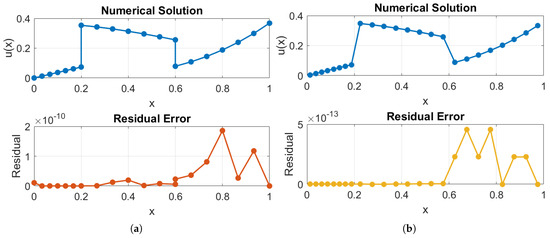
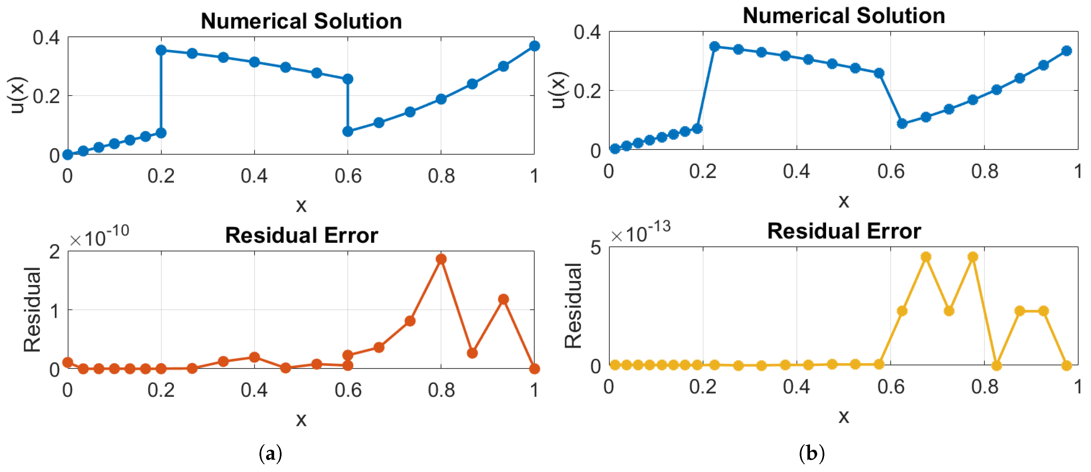
The initial, boundary, and interface conditions are taken from Example 1. Table 11 presents the residual errors obtained by MQ-RBF and HWCM for different values of M and ρ. Since the exact solution is not available for this problem, the accuracy of both numerical schemes is evaluated through the residual error. It can be observed that both methods yield very small residuals (ranging from ${10}^{-9}$ to ${10}^{-13}$), demonstrating high numerical accuracy. Furthermore, HWCM exhibits comparatively more stable residual behavior as the discretization parameters are refined. Additionally, the residual errors and numerical solutions have been plotted in graphical form, as shown in Figure 17.

Table 11. Residual errors for Example 4 using MQ-RBF and HWCM.

$\mathcal{M}$	$\mathbf{\Delta }\mathit{t}$	$\mathit{\rho }=0.6$	$\mathit{\rho }=0.8$
		Residual Error	Residual Error
MQ-RBF
6	0.5/6	$2.2737\times {10}^{-13}$	$5.6843\times {10}^{-14}$
12	0.5/12	$1.0004\times {10}^{-11}$	$9.5497\times {10}^{-12}$
18	0.5/18	$1.8576\times {10}^{-10}$	$1.2074\times {10}^{-10}$
24	0.5/24	$6.0352\times {10}^{-9}$	$2.5186\times {10}^{-9}$
HWCM
6	0.5/6	$4.5475\times {10}^{-13}$	$4.5475\times {10}^{-13}$
12	0.5/12	$2.2737\times {10}^{-13}$	$4.5475\times {10}^{-13}$
24	0.5/24	$6.8212\times {10}^{-13}$	$4.5475\times {10}^{-13}$
48	0.5/48	$1.8190\times {10}^{-12}$	$1.1369\times {10}^{-12}$

Figure 17. (a) Numerical solution and residual error using MQ-RBF. (b) Numerical solution and residual error using HWCM are presented for $M=18$ and $\rho =0.8$.

8. Conclusions

In conclusion, this study developed and analyzed two numerical approaches for solving time-fractional double interface problems. The Haar wavelet collocation method consistently showed higher accuracy and efficiency than the meshfree technique based on radial basis functions. Both methods effectively handle constant and variable coefficients, as well as discontinuities and singularities. Discontinuities and sharp changes at the interfaces are accurately captured by the proposed schemes, demonstrating their robustness for interface-dominated problems. The Haar wavelet approach, in particular, stands out due to its localized and piecewise structure, which enables sharper resolution of irregular features near the interfaces. From a physical perspective, the time-fractional formulation captures memory-dependent transport phenomena in layered and heterogeneous media, where double interfaces represent realistic composite structures. The numerical results show that fractional order plays a significant role in the governing behavior of the solution, especially near the interfaces, reflecting anomalous diffusion effects observed in complex materials. The novelty of this work lies in the unified and accurate application of Haar wavelet collocation and meshless radial basis function methods to time-fractional double interface problems with both constant and variable coefficients, without requiring mesh generation or interface smoothing. Linear problems are solved using Gaussian elimination, and numerical experiments confirm the effectiveness and stability of both schemes, with the Haar wavelet method emerging as the most robust and precise. The two- and three-dimensional graphical results for different fractional orders clearly illustrate the ability of the proposed methods to track discontinuities and sharp variations at the interfaces. For future research, extending these techniques to higher order time-fractional derivatives and to two- and three-dimensional interface problems remains an open and promising direction.

References

- Asif, M.; Riaz, M.B.; Bilal, F. A hybrid meshless collocation approach for capturing solution and gradient jumps in 1D telegraph double-interface model with highly discontinuous coefficients. Results Appl. Math. 2026, 29, 100685. [Google Scholar] [CrossRef] [Scilit]
- Bilal, F.; Asif, M.; Shakeel, M.; Popa, I.-L. RBF-Based Meshless Collocation Method for Time-Fractional Interface Problems with Highly Discontinuous Coefficients. Math. Comput. Appl. 2025, 30, 133. [Google Scholar] [CrossRef] [Scilit]
- Faheem, M.; Asif, M.; Haider, N.; Amin, R. Hybrid Haar wavelet and meshfree methods for hyperbolic double interface problems: Numerical implementations and comparative performance analysis. Partial Differ. Equ. Appl. Math. 2024, 11, 100773. [Google Scholar] [CrossRef] [Scilit]
- Asif, M.; Gul, J.; Shakeel, M.; Popa, I.-L. A Hybrid Numerical Framework Based on Radial Basis Functions and Finite Difference Method for Solving Advection–Diffusion–Reaction-Type Interface Models. Math. Comput. Appl. 2025, 31, 1. [Google Scholar] [CrossRef] [Scilit]
- Layton, A.T. Using integral equations and the immersed interface method to solve immersed boundary problems with stiff forces. Comput. Fluids 2009, 38, 266–272. [Google Scholar] [CrossRef] [Scilit]
- Brauner, N.M.; Maron, D.M.; Rovinsky, J. A two-fluid model for stratified flows with curved interfaces. Int. J. Multiph. Flow 1998, 24, 975–1004. [Google Scholar] [CrossRef] [Scilit]
- Babuska, I. The finite element method for elliptic equations with discontinuous coefficients. Computing 1970, 5, 207–213. [Google Scholar] [CrossRef] [Scilit]
- Aziz, I.; Islam, S.U.; Haider, N. Meshless and multi-resolution collocation techniques for steady state interface models. Int. J. Comput. Methods 2018, 15, 1750073. [Google Scholar] [CrossRef] [Scilit]
- Haider, N.; Aziz, I. Meshless and multi-resolution collocation techniques for parabolic interface models. Appl. Math. Comput. 2018, 335, 313–332. [Google Scholar] [CrossRef] [Scilit]
- Asif, M.; Farooq, U.; Riaz, M.B.; Bilal, F.; Haider, N. Numerical assessment of hyperbolic type double interface problems via Haar wavelets. Partial Differ. Equ. Appl. Math. 2024, 10, 100665. [Google Scholar] [CrossRef] [Scilit]
- Asif, M.; Bilal, F.; Bilal, R.; Haider, N. An efficient algorithm for the numerical solution of telegraph interface model with discontinuous coefficients via Haar wavelets. Alex. Eng. J. 2023, 72, 275–285. [Google Scholar] [CrossRef] [Scilit]
- Rana, G.; Asif, M.; Haider, N.; Bilal, R.; Ahsan, M.; Al-Mdallal, Q.; Jarad, F. A modified algorithm based on Haar wavelets for the numerical simulation of interface models. J. Funct. Spac. 2022, 2022, 1541486. [Google Scholar] [CrossRef] [Scilit]
- Asif, M.; Bilal, F.; Haider, N.; Jarad, F. Robust numerical techniques for modeling telegraph equations in multi-scale and heterogeneous environments. J. Appl. Math. Comput. 2025, 6585–6620. [Google Scholar] [CrossRef] [Scilit]
- Asif, M.; Gul, T.; Riaz, M.B.; Bilal, F. Solution of nonlinear telegraph equation with discontinuities along the transmission line using meshless collocation method. Partial Differ. Equ. Appl. Math. 2025, 14, 101219. [Google Scholar] [CrossRef] [Scilit]
- Asif, M.; Akhtar, N.; Khan, F.; Bilal, F.; Popa, I.-L. Numerical Treatment of Hyperbolic-Type Problems with Single and Double Interfaces via Meshless Method. Axioms 2025, 14, 621. [Google Scholar] [CrossRef] [Scilit]
- Ahmad, M.; Islam, S.U.; Ullah, B. Local radial basis function collocation method for stokes equations with interface conditions. Eng. Anal. Bound. Elem. 2020, 119, 246–256. [Google Scholar] [CrossRef] [Scilit]
- Ahmad, M.; Islam, S.U.; Larsson, E. Local meshless methods for second order elliptic interface problems with sharp corners. J. Comput. Phys. 2020, 416, 109500. [Google Scholar] [CrossRef] [Scilit]
- Ahmed, K.K.; Ahmed, H.M.; Badra, N.M.; Rabie, W.B. Optical solitons retrieval for an extension of novel dual-mode of a dispersive non-linear Schrödinger equation. Optik 2024, 307, 171835. [Google Scholar] [CrossRef] [Scilit]
- Alraddadi, I.; Alsharif, F.; Malik, S.; Ahmad, H.; Radwan, T.; Ahmed, K.K. Innovative soliton solutions for a (2+1)-dimensional generalized KdV equation using two effective approaches. AIMS Math. 2024, 9, 34966–34980. [Google Scholar] [CrossRef] [Scilit]
- Alam, N.; Ullah, M.S.; Nofal, T.A.; Ahmed, H.M.; Ahmed, K.K.; AL-Nahhas, M.A. Novel dynamics of the fractional KFG equation through the unified and unified solver schemes with stability and multistability analysis. Nonlinear Eng. 2024, 13, 20240034. [Google Scholar] [CrossRef] [Scilit]
- Samir, I.; Ahmed, H.M.; Emadifar, H.; Ahmed, K.K. Traveling and soliton waves and their characteristics in the extended (3+1)-dimensional Kadomtsev Petviashvili equation in fluid. Partial Differ. Equ. Appl. Math. 2025, 14, 101146. [Google Scholar] [CrossRef] [Scilit]
- Khalifa, A.; Ahmed, H.; Badra, N.; Rabie, W. Unveiling of highly dispersive dual-solitons and modulation instability analysis for dual-mode extension of a non-linear Schrödinger equation. Contemp. Math. 2024, 542, 5358–5381. [Google Scholar] [CrossRef] [Scilit]
- Zada, L.; Aziz, I. The numerical solution of fractional Korteweg-de Vries and Burgers’ equations via Haar wavelet. Math. Methods Appl. Sci. 2021, 44, 10564–10577. [Google Scholar] [CrossRef] [Scilit]
- Oldham, K.B. Fractional differential equations in electrochemistry. Adv. Eng. Softw. 2010, 41, 9–12. [Google Scholar] [CrossRef] [Scilit]
- Koeller, R. Applications of fractional calculus to the theory of viscoelasticity. J. Appl. Mech. 1984, 51, 299–307. [Google Scholar] [CrossRef] [Scilit]
- Diethelm, K.; Ford, N.J. Analysis of fractional differential equations. J. Math. Anal. 2002, 265, 229–248. [Google Scholar] [CrossRef] [Scilit]
- Zada, L.; Aziz, I. Numerical solution of fractional partial differential equations via Haar wavelet. Numer. Methods Partial Differ. Equ. 2022, 38, 222–242. [Google Scholar] [CrossRef] [Scilit]
- Shakeel, M.; Hussain, I.; Ahmad, H.; Thounthong, P.; Zhang, Y. Meshless technique for the solution of time-fractional partial differential equations having real-world applications. J. Funct. Spcs. 2020, 2020, 8898309. [Google Scholar] [CrossRef] [Scilit]
- Mehnaz, S.; Khan, M.N.; Ahmad, I.; Ahmad, H. Local meshless collocation scheme for numerical simulation of space fractional PDE. Therm. Sci. 2020, 27, 101–109. [Google Scholar]
- Manzoor, H.; Siraj, H.; Ahmad, I.; Ahmad, H. Meshless spectral method for solution of time-fractional coupled KdV equations. Appl. Math. Comput. 2020, 341, 321–334. [Google Scholar]
- Bin Jebreen, H.; Cattani, C. Solving time-fractional partial differential equation using Chebyshev cardinal functions. Axioms 2022, 11, 642. [Google Scholar] [CrossRef] [Scilit]
- Rahma, A.M.; Banan, M. Adaptive Technique for Solving 1-D Interface Problems of Fractional Order. Int. J. Appl. Comput. Math. 2022, 8, 214. [Google Scholar] [CrossRef] [Scilit]
- Wang, T.; Chen, Y. Nitsche-XFEM for a time fractional diffusion interface problem. Sci. China Math. 2024, 67, 665–682. [Google Scholar] [CrossRef] [Scilit]
- Lepik, Ü.; Hein, H. Haar Wavelets: With Applications; Springer: Berlin/Heidelberg, Germany, 2014; pp. 7–20. [Google Scholar]
- Asif, M.; Haider, N.; Al-Mdallal, Q.; Khan, I. A Haar wavelet collocation approach for solving one and two-dimensional second-order linear and nonlinear hyperbolic telegraph equations. Numer. Methods Partial Differ. Equ. 2020, 36, 1962–1981. [Google Scholar] [CrossRef] [Scilit]
- Maleknejad, K.; Lotfi, T.; Mahdiani, K. Numerical solution of first kind Fredholm integral equations with wavelets-Galerkin method (WGM) and wavelets precondition. Appl. Math. Comput. 2007, 186, 794–800. [Google Scholar] [CrossRef] [Scilit]
- Amin, R.; Shah, K.; Awais, M.; Ibrahim, M.; Sooppy, K.; Wojciech, S. Existence and solution of third-order integro-differential equations via Haar wavelet method. Fractals 2023, 31, 2340037. [Google Scholar] [CrossRef] [Scilit]
- Amin, R.; Hadi, F.; Altanji, M.; Sooppy, K.; Wojciech, S. Solution of variable-order nonlinear fractional differential equations using Haar wavelet collocation technique. Fractals 2023, 31, 2340022. [Google Scholar] [CrossRef] [Scilit]
- Hsiao, C.-H. State analysis of linear time delayed systems via Haar wavelets. Math. Comput. Simul. 1997, 44, 457–470. [Google Scholar] [CrossRef] [Scilit]
- Chen, C.F.; Hsiao, C.-H. Haar wavelet method for solving lumped and distributed-parameter systems. IEE Proc.-Control Theory Appl. 1997, 144, 87–94. [Google Scholar] [CrossRef] [Scilit]
- Lepik, Ü. Haar wavelet method for nonlinear integro-differential equations. Appl. Math. Comput. 2006, 176, 324–333. [Google Scholar] [CrossRef] [Scilit]
- Lepik, Ü.; Tamme, E. Solution of nonlinear Fredholm integral equations via the Haar wavelet method. Proc. Est. Acad. Sci. Phys. Math. 2007, 56, 17–27. [Google Scholar] [CrossRef] [Scilit]
- Lepik, Ü. Solving PDEs with the aid of two-dimensional Haar wavelets. Comput. Math. Appl. 2011, 61, 1873–1879. [Google Scholar] [CrossRef] [Scilit]
- Lepik, Ü. Numerical solution of evolution equations by the Haar wavelet method. Appl. Math. Comput. 2007, 185, 695–704. [Google Scholar] [CrossRef] [Scilit]
- Lepik, Ü. Application of the Haar wavelet transform to solving integral and differential equations. Proc. Estonian Acad. Sci. Phys. Math. 2007, 56, 28–46. [Google Scholar] [CrossRef] [Scilit]
- Lepik, Ü. Haar wavelet method for solving higher order differential equations. Int. J. Math. Comput. 2008, 1, 84–94. [Google Scholar]
- Wu, J. A wavelet operational method for solving fractional partial differential equations numerically. Appl. Math. Comput. 2009, 214, 31–40. [Google Scholar] [CrossRef] [Scilit]
- Asif, M.; Bilal, F.; Khan, I. Extension of Haar wavelet technique for numerical solution of three-dimensional linear and nonlinear telegraph equations. Partial Differ. Equ. Appl. Math. 2023, 9, 100618. [Google Scholar] [CrossRef] [Scilit]
- Majak, J.; Ratas, M.; Karjust, K.; Shvartsman, B. Higher order Haar wavelet method for solving differential equations. In Wavelet Theory; IntechOpen: London, UK, 2020; p. 349. [Google Scholar]
- Majak, J.; Shvartsman, B.; Ratas, M.; Bassir, D.; Pohlak, M.; Karjust, K.; Eerme, M. Higher-order Haar wavelet method for vibration analysis of nanobeams. Mater. Today Commun. 2020, 25, 101290. [Google Scholar] [CrossRef] [Scilit]
- Shakeel, M.; Parveen, S.; Islam, S.; Hussain, I. Numerical solution and characteristic study of time-fractional shocks collision. Phys. Scr. 2021, 96, 045214. [Google Scholar] [CrossRef] [Scilit]
- Hardy, R.L. Multiquadric equations of topography and other irregular surfaces. J. Geophys. Res. 1971, 76, 1904–1915. [Google Scholar] [CrossRef] [Scilit]
- Kansa, E.J. Multiquadrics—A scattered data approximation scheme with applications to computational fluid-dynamics I: Surface approximations and partial derivative estimates. Comput. Math. Appl. 1990, 19, 147–161. [Google Scholar] [CrossRef] [Scilit]
- Franke, C.; Schaback, R. Solving partial differential equations by collocation using radial basis functions. Appl. Math. Comput. 1998, 93, 73–82. [Google Scholar] [CrossRef] [Scilit]
- Hon, Y.C.; Mao, X.Z. An efficient numerical scheme for Burgers’ equation. Appl. Math. Comput. 1998, 95, 37–50. [Google Scholar] [CrossRef] [Scilit]
- Hu, J.; Ying, C.; Li, S.; Jin, Z.; Chao, X.; Wang, X. Analyzing the Transient Process and the Realizability of Fractional Systems via Intermittent Control. Fractal Fract. 2025, 9, 184. [Google Scholar] [CrossRef] [Scilit]
- Hu, J.; Li, S.; Jin, Z.; Chao, X. Studying the transient process of an intermittent control system from its response property. Commun. Nonlinear Sci. Numer. Simul. 2024, 139, 108309. [Google Scholar] [CrossRef] [Scilit]
- Hu, J. Analyzing the Approximate Error and Applicable Condition of the Fractional Reduced Differential Transform Method. Symmetry 2024, 16, 912. [Google Scholar] [CrossRef] [Scilit]
- Hu, J.; Wu, Y.; Li, S.; Li, G.; Chao, X. Synchronization Transient and Stability Analysis of Fractional Neural Networks with Intermittent Control Based on Its Memory Characteristic. Asian J. Control 2025. [Google Scholar] [CrossRef] [Scilit]
- Ahsan, M.; Tran, T.; Hussain, I. A multiresolution collocation method and its convergence for Burgers’ type equations. Math. Methods Appl. Sci. 2023, 46, 11702–11725. [Google Scholar] [CrossRef] [Scilit]
- Mannan, M.A.; Rahman, M.R.; Akter, H.; Nahar, N.; Mondal, S. A study of Banach fixed point theorem and its applications. Am. J. Comput. Math. 2021, 11, 157–174. [Google Scholar] [CrossRef]
- Palais, R.S. A simple proof of the Banach contraction principle. J. Fixed Point Theory Appl. 2007, 2, 221–223. [Google Scholar] [CrossRef] [Scilit]
- LeVeque, R.J. Finite Difference Methods for Ordinary and Partial Differential Equations: Steady-State and Time-Dependent Problems; SIAM: Philadelphia, PA, USA, 2007. [Google Scholar]
Disclaimer/Publisher’s Note: The statements, opinions and data contained in all publications are solely those of the individual author(s) and contributor(s) and not of MDPI and/or the editor(s). MDPI and/or the editor(s) disclaim responsibility for any injury to people or property resulting from any ideas, methods, instructions or products referred to in the content. |
© 2026 by the authors. Licensee MDPI, Basel, Switzerland. This article is an open access article distributed under the terms and conditions of the Creative Commons Attribution (CC BY) license.