The Structure of the Route to the Period-Three Orbit in the Collatz Map

Abstract

The Collatz map is investigated from a nonlinear-dynamics perspective with emphasis on the structure of its iterative orbits. By embedding integers within Sharkovsky’s ordering, odd initial values are shown to be sufficient for a complete characterization of dynamics. A “direction-phase” decomposition is introduced to separate iterative orbits into upward and downward phases, yielding a family of recursive functions parameterized by the number of upward phases. This formulation reveals a logarithmic scaling relation between the total iteration count and the initial value, confirming finite-time convergence to the period-three orbit. The Collatz dynamics is further shown to be dynamically equivalent to a binary shift map, whose ergodicity implies inevitable evolution toward attractors, thereby reinforcing convergence. Numerical analysis indicates that attraction basins follow a power-law distribution and display pronounced self-similarity. Moreover, odd integers grouped by upward-phase counts are found to follow Gamma statistics. Beyond its research implications, the framework provides a concise pedagogical case study illustrating how nonlinear dynamics, symbolic dynamics, and statistical characterization can be integrated to analyze a classical discrete problem.

1. Introduction

Dynamic systems exhibiting behaviors ranging from periodic oscillations to chaotic phenomena are ubiquitous in nature and engineering [1,2,3,4,5,6]. Nonlinear dynamics provides a systematic framework for analyzing and predicting the evolution of such complex systems [7]. Discrete dynamical systems, governed by difference equations and characterized by iterative state transitions, serve as effective models for phenomena including population dynamics, digital signal processing, and economic cycles [8]. These systems exhibit diverse behaviors such as periodicity, chaos, bifurcations, and fractal patterns [9,10,11]. Their theoretical significance and practical relevance have established discrete dynamical systems as a central focus in nonlinear-dynamics research [12,13,14,15,16,17,18,19,20,21,22,23].

In nonlinear dynamics, Sharkovsky’s theorem [24,25] and Li–Yorke’s theorem [26] are foundational results. Sharkovsky’s theorem establishes the coexistence of periodic solutions in one-dimensional discrete maps through Sharkovsky’s ordering [27], showing that the existence of certain periodic orbits implies the existence of others. In particular, the presence of a period-three orbit guarantees orbits of all integer periods. Li–Yorke’s theorem, encapsulated by the dictum “period-three implies chaos” [26], both reframes Sharkovsky’s insight and provides a rigorous notion of chaos. Chaotic dynamics is characterized by extreme sensitivity to initial conditions: arbitrarily small differences in initial states can grow exponentially, undermining long-term predictability [28,29]. The recognition of deterministic chaos challenges classical expectations that determinism necessarily implies predictability and reshapes the conceptual understanding of complex nonlinear behavior [30,31,32]. Importantly, the “period-three implies chaos” principle applies to continuous self-maps of an interval and does not, in general, extend to purely discrete maps.

In this study, the Collatz map is analyzed as a discrete dynamical system, using methods from nonlinear dynamics to investigate the structure of its iterative orbits and its statistical behavior [33]. Also known as the Collatz conjecture (or the $3X+1$ problem), it is renowned for its simple formulation [34] and unresolved status [35,36,37,38,39,40,41]. The conjecture asserts that repeated application of the transformation

$$X=\left\{\begin{array}{cc}3X+1,\hfill & \mathrm{if}X\mathrm{is}\mathrm{odd};\hfill \\ X/2,\hfill & \mathrm{if}X\mathrm{is}\mathrm{even},\hfill \end{array}\right.$$

(1)

eventually maps any positive integer X to the cycle $\{4,2,1\}$.

Significant progress has been made in characterizing the probabilistic behavior of Collatz orbits. Early work by Crandall [42] established constraints linking the map to Diophantine equations, and subsequent studies, including Krasikov’s statistical approximations [43], further developed probabilistic approaches. Recently, Tao [40] employed random-walk methods together with skew distributions on cyclic groups to prove convergence for “almost all” integers in the sense of logarithmic density, thereby providing strong heuristic support for the conjecture. More recently, in 2024, Polli et al. [44] carried out a systematic study of hailstone sequences using tools from nonlinear dynamics and time-series analysis—see also references therein. Although the Collatz map is a deterministic arithmetic system, their results indicate that its orbits display pronounced randomness-like behavior, exhibit global features consistent with geometric Brownian motion, and contain identifiable short- and medium-range correlations. These findings highlight connections between arithmetic dynamical systems and methods commonly used in statistical physics.

The Collatz conjecture involves two requirements: (i) uniqueness, meaning that $\{4,2,1\}$ is the only periodic cycle; and (ii) convergence, meaning that every positive integer reaches this cycle after finitely many iterations. Establishing both properties would resolve the conjecture. However, a universal proof remains elusive despite extensive computational verification. In particular, Barina’s studies report verification for all integers $X\le 2^{68}\approx 2.9515\times {10}^{20}$ in 2021 [45], and an expanded bound of $X\le 2^{71}\approx 2.3612\times {10}^{21}$ by 2025 [46] (see references therein), reflecting continued progress in large-scale verification.

In this work, Sharkovsky’s ordering is employed to represent integers, and it is proved that a complete dynamics characterization of the Collatz map can be obtained by focusing solely on odd initial values. A “direction-phase” decomposition is introduced to classify iterations into upward and downward phases, leading to a family of recursive functions parameterized by the number of upward phases. This formulation reveals a logarithmic relationship between the number of iteration steps and the initial value, and it demonstrates finite-time convergence to the period-three orbit $\{4,2,1\}$. In addition, an equivalence between the Collatz map and a binary shift map is established. The ergodicity of the binary shift map [47] implies inevitable evolution toward attractors, thereby reinforcing convergence. Numerical analysis indicates that attraction basins follow power-law distributions and exhibit pronounced self-similarity, while odd integers grouped by upward-phase counts approximately follow Gamma distributions. Beyond its implications for rigorous analysis of the Collatz conjecture, the framework provides a pedagogically useful model for undergraduate and graduate courses in nonlinear dynamics, number theory, computational physics, and computational mathematics, illustrating decomposition strategies for complex maps and parameterization techniques.

The paper is organized as follows. Section 2 defines the Collatz map and introduces the concept of “direction phases”. Section 3 develops the theoretical framework. Section 4 presents the numerical validation. Section 5 concludes and discusses the remaining open challenges.

2. The Collatz Map and Definition of Direction Phases

For brevity, the map in Equation (1) is written as

$$X_n=M\left(X_{n-1}\right)=M^n\left(X_0\right),$$

(2)

where $n, X_n\in {\mathbb{Z}}^{+}$. The Collatz conjecture states that

$$\underset{n\to \infty }{lim}{M}^n\left(X_0\right)=\{4,2,1\}\mathrm{for}\mathrm{all}{X}_0\in {\mathbb{Z}}^{+},$$

(3)

that is, every trajectory eventually enters the period-three orbit $\{4,2,1\}$.

To formalize the dynamics, the notion of “direction phases” is introduced [48]:

$$\left\{\begin{array}{cc}{P}_{\uparrow }\left(n\right)=1,\hfill & \mathrm{if}{X}_{n+1}>X_n(\mathrm{up}\mathrm{phase}),\hfill \\ P_{\downarrow }\left(n\right)=-1,\hfill & \mathrm{if}{X}_{n+1}<X_n(\mathrm{down}\mathrm{phase}).\hfill \end{array}\right.$$

(4)

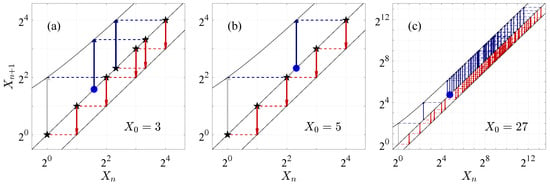
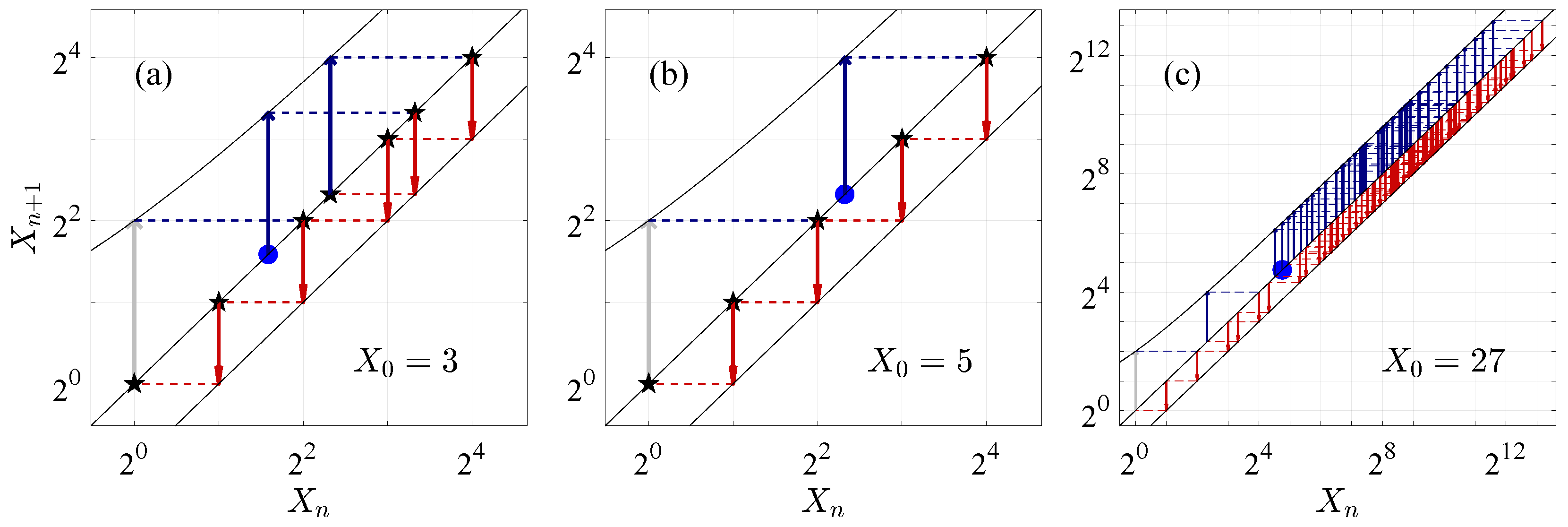
Let $N_{\uparrow }$ and $N_{\downarrow }$ denote the numbers of up and down phases, respectively, counted before the orbit enters $\{1,4,2\}$. For example, as shown in Figure 1a–c, trajectories with $X_0=3,5,27$ yield $(N_{\uparrow },N_{\downarrow })=(2,5),(1,4),(41,70)$, respectively. The quantities $N_{\uparrow }$ and $N_{\downarrow }$ coincide with the numbers of odd and even terms, respectively, in the iteration sequence from $X_0\ne 1$ until the first occurrence of 2. The total number of iterations is $N=N_{\uparrow }+N_{\downarrow }$, so that $M^N\left(X_0\right)=1$.

Figure 1. Cobweb plot of the orbits for different initial values $X_0$ on a log–log scale.

The Collatz map extends to all integers as

$$X_{n+1}=\left\{\begin{array}{cc}3X_n+\mathrm{sgn}\left(X_n\right),\hfill & \mathrm{if}{X}_n\mathrm{is}\mathrm{odd},\hfill \\ X_n/2,\hfill & \mathrm{if}{X}_n\mathrm{is}\mathrm{even},\hfill \end{array}\right.$$

(5)

where $X_n\in \mathbb{Z}$ and $\mathrm{sgn}$ denotes the sign function. The extended conjecture is then

$$\underset{n\to \infty }{lim}{M}^n\left(X_0\right)=\left\{\begin{array}{cc}\{-4,-2,-1\},\hfill & X_0\in {\mathbb{Z}}^{-},\hfill \\ \left\{0\right\},\hfill & X_0=0,\hfill \\ \{4,2,1\},\hfill & X_0\in {\mathbb{Z}}^{+}.\hfill \end{array}\right.$$

(6)

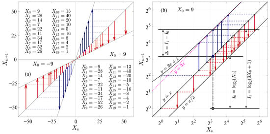
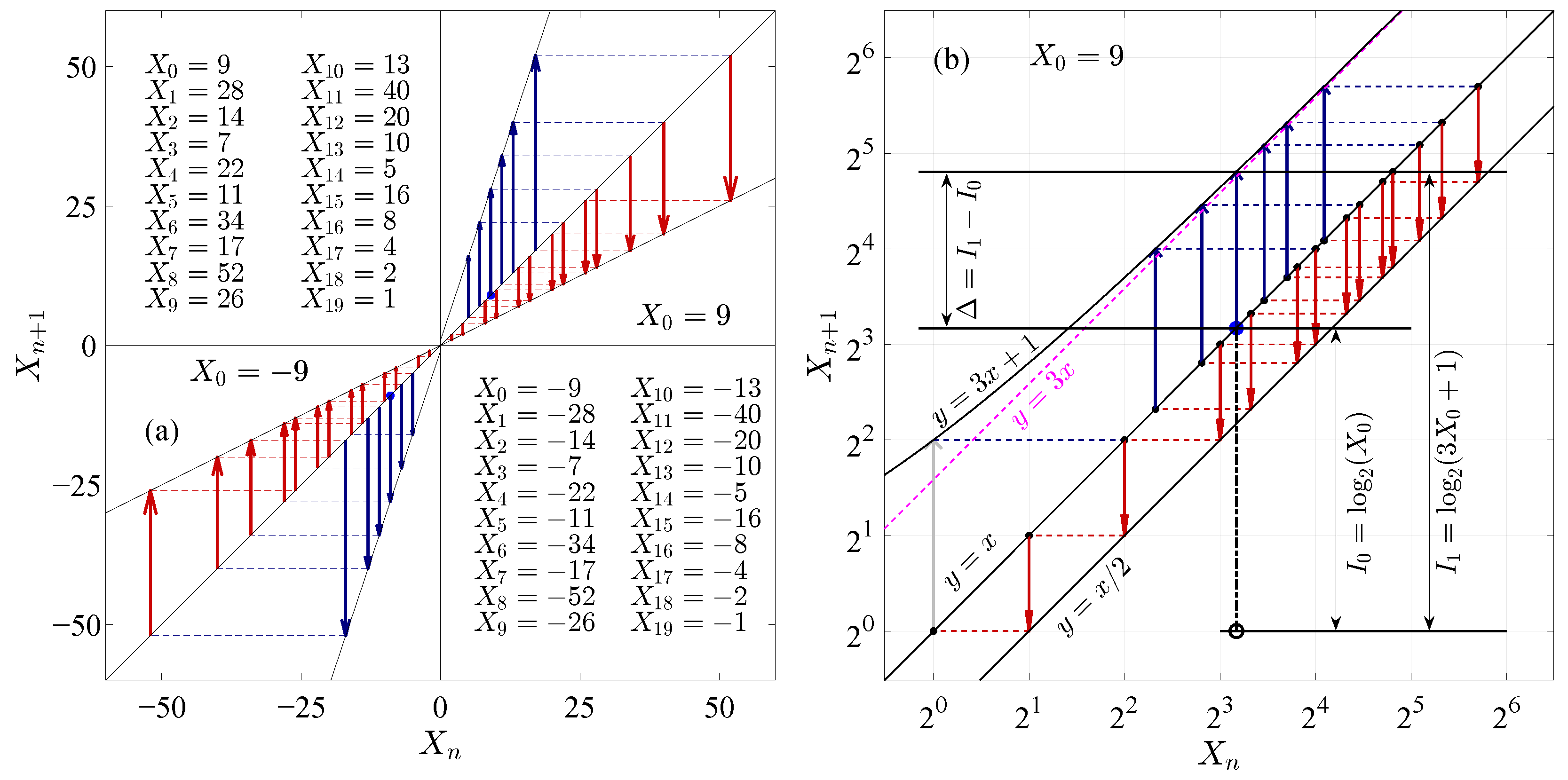
Figure 2a shows symmetric trajectories for $X_0=\pm 9$, which converge to $\pm 1$. The analysis in this paper focuses on $X_0\in {\mathbb{Z}}^{+}$, and the theoretical framework is developed in the subsequent sections.

Figure 2. (a) Cobweb plot of the orbits with $X_0=\pm 9$. The second and fourth quadrants display the iterative sequences for $X_0=9$ and $X_0=-9$, respectively. (b) Iterative trajectory for $X_0=9$ from panel (a) shown on a double-logarithmic scale. Note that $I_0={log}_2\left(X_0\right)\approx 3.1699$, $I_1={log}_2(3X_0+1)\approx 4.8074$, and $\Delta =I_1-I_0\approx 1.6375$.

3. Theoretical Analysis

Two infinite-dimensional vectors are defined as

$$\mathit{B}=\left[2^0,2^1,2^2,\dots ,2^m,\dots \right],$$

(7)

$$\mathit{O}=\left[3,5,7,\dots ,2n+1,\dots \right].$$

(8)

The matrix $\mathit{D}={\mathit{B}}^{\mathit{T}}\mathit{O}$ then has the explicit form

$$\mathit{D}=\left[\begin{array}{ccccc}3·2^0& 5·2^0& \dots & (2n+1)·2^0& \dots \\ 3·2^1& 5·2^1& \dots & (2n+1)·2^1& \dots \\ ⋮& ⋮& \ddots & ⋮& ⋮\\ 3·2^m& 5·2^m& \dots & (2n+1)·2^m& \dots \\ ⋮& ⋮& \ddots & ⋮& ⋮\end{array}\right].$$

(9)

Let $\mathbb{B}$, $\mathbb{O}$, and $\mathbb{D}$ denote the sets formed by the elements of $\mathit{B}$, $\mathit{O}$, and $\mathit{D}$, respectively. Under Sharkovsky’s ordering [24], the union $\mathbb{D}\cup \mathbb{B}$ coincides with ${\mathbb{Z}}^{+}$.

If $X_0=2^m\in \mathbb{B}$, then $M^m\left(X_0\right)=1$, and the corresponding trajectory has $N_{\uparrow }=0$ and $N=N_{\downarrow }=m$. If $X_0=(2n+1)·2^m\in \mathbb{D}$, then $M^m\left(X_0\right)=2n+1\in \mathbb{O}$. Consequently, the analysis of the Collatz map can be restricted to odd initial values $X_0\in \mathbb{O}$.

3.1. Estimation of Iteration Steps

• Case I: $N_{\uparrow }=1$. For $X_0\in \mathbb{O}$ with $N_{\uparrow }=1$, the following representation holds:

$$X_0=F_1\left(m\right)={\displaystyle \frac{2^m-1}{3}}\in \mathbb{O}(m>2).$$

(10)

The condition $F_1\left(m\right)\in \mathbb{O}$ is satisfied if and only if $m=2p$, which yields

$$X_0=F_1\left(p\right)={\displaystyle \frac{4^p-1}{3}},p\ge 2.$$

(11)

A convenient recursion follows

$$F_1\left(p\right)=4^{p-1}+F_1(p-1).$$

(12)

If $F_1\left(1\right)\equiv 1\in \mathbb{B}$ is defined by substituting $p=1$ into Equation (11), then Equations (11) and (12) generate the same sequence for all $p\ge 2$. From Equation (11), the total number of iterations required for convergence is

$$N_1=N_{\uparrow }+N_{\downarrow }=1+2p=1+{log}_2(3X_0+1).$$

(13)

• Case II: $N_{\uparrow }=2$. For $X_0\in \mathbb{O}$ with $N_{\uparrow }=2$, one obtains

$$X_0=F_2(p,k_1)={\displaystyle \frac{2^{k_1}{F}_1\left(p\right)-1}{3}}(k_1\ge 1).$$

(14)

In this case,

$$F_2(p,k_1)=F_2(p,k_1-2)+2^{k_1-2}{F}_1\left(p\right).$$

(15)

• General case: $N_{\uparrow }=s$. For $X_0\in \mathbb{O}$ with $N_{\uparrow }=s$, define recursively

$$X_0=F_s(p,k_{s-1})={\displaystyle \frac{2^{k_{s-1}}{F}_{s-1}(p,k_{s-2})-1}{3}}.$$

(16)

The function $F_s$ satisfies the recursion

$$F_s(p,k_{s-1})=F_s(p,k_{s-1}-2)+2^{k_{s-1}-2}{F}_{s-1}(p,k_{s-2}).$$

(17)

An explicit form can be obtained. For example, $F_4$ can be written as

$$\begin{array}{cc}\hfill F_4(p,k_3)& ={\displaystyle \frac{2^{k_3}\left\{\frac{2^{k_2}\left[\frac{2^{k_1}\left(\frac{4^p-1}{3}\right)-1}{3}\right]-1}{3}\right\}-1}{3}}\hfill \\ \hfill & ={\displaystyle \frac{2^{2p+k_1+k_2+k_3}}{3^4}}-{\displaystyle \frac{2^{k_1+k_2+k_3}}{3^4}}-{\displaystyle \frac{2^{k_2+k_3}}{3^3}}-{\displaystyle \frac{2^{k_3}}{3^2}}-{\displaystyle \frac{1}{3}}.\hfill \end{array}$$

(18)

The general form of $F_s$ is

$$F_s={\displaystyle \frac{1}{3^s}}\left(2^{K_s}-\sum _{i=1}^{s-1}{3}^{s-1-i}{2}^{K_i}-3^{s-1}\right)={\displaystyle \frac{1}{3^s}}\left(2^{K_s}-\sum _{i=0}^{s-1}{3}^{s-1-i}{2}^{K_i}\right),$$

(19)

which depends on the independent variables s and p, where

$$K_s=2p+K_{s-1},K_{s-l}=\sum _{j=l}^{s-1}{k}_j\mathrm{for}l=1,2,\dots ,s-1,K_0=0.$$

(20)

Since $k_j\in {\mathbb{Z}}^{+}$ for $1\le j\le s-1$, it follows that $K_s>K_{s-1}>\dots >K_1\ge 1$.

Equation (19) implies that if $F_s$ is an integer, then $F_s\in \mathbb{O}$. By writing $3=2+1$ and applying the binomial expansion, Equation (19) can be rewritten as

$$F_s={\displaystyle \frac{1}{3^s}}\left[2^{K_s}-\sum _{i=0}^{s-1}\sum _{j=0}^{s-1-i}{\displaystyle \frac{\Gamma (s-i)}{\Gamma (j+1)\Gamma (s-i-j)}}{2}^{s-1-i-j+K_i}\right],$$

(21)

where the binomial coefficients are expressed in terms of the Gamma function.

For compactness, Equation (19) can also be rewritten as an inner product,

$$F_s={\mathit{a}}_s·{\mathit{b}}_s,$$

(22)

with

$$\begin{array}{cc}\hfill {\mathit{a}}_s& ={\displaystyle \frac{1}{3^s}}\left[1,-3^0,-3^1,\dots ,-3^{s-3},-3^{s-2},-3^{s-1}\right],\hfill \\ \hfill {\mathit{b}}_s& =\left[2^{K_s},2^{K_{s-1}},2^{K_{s-2}},\dots ,2^{K_2},2^{K_1},2^{K_0}\right],\hfill \end{array}$$

(23)

where the number of up phases $s=N_{\uparrow }$ determines the dimension of the vectors. A related construction was reported in Ref. [34]. If $X_0=F_s$, then $N_{\downarrow }=K_s$ and the total iteration count satisfies $N_s=s+K_s$, so that $X_{N_s}=M^{N_s}\left(X_0\right)=1$. The following discussion estimates the total number of iterations $N_s$.

To visually demonstrate the idea of estimation, Figure 2b presents a cobweb plot for the orbit with initial value $X_0=9$ on a log–log scale. In this representation, the downward red-arrow segments have equal length in the double-logarithmic coordinate system because the lines $y=x$ and $y=x/2$ are parallel in log–log coordinates, and the corresponding segment length equals 1. By contrast, the upward blue segments located between $y=3x+1$ and $y=x$ do not have exactly equal length because $y=3x+1$ and $y=x$ are not parallel in double-logarithmic coordinates. Since these two curves become approximately parallel for sufficiently large x, the lengths of the upward segments are approximately equal. Therefore, the total length of the upward segments $\mathcal{L}$ can then be estimated as

$$\mathcal{L}=s\Delta =s(I_1-I_0)=s\left[{log}_2(3X_0+1)-{log}_2\left(X_0\right)\right]=s{log}_2\left(3+{\displaystyle \frac{1}{X_0}}\right),$$

(24)

where $\Delta$ denotes the difference between the exponents indicated in Figure 2b. Logically, if the iteration starting from $X_0$ eventually enters the period-three orbit, then the total length of the upward segments, along with the initial distance $I_0$, equals the total length of the downward segments. That is, the upward and downward trajectories form a closed loop. This balance yields

$$N_{\downarrow }=\lfloor \mathcal{L}+I_0\rceil =\lfloor s(I_1-I_0)+I_0\rceil ,$$

(25)

where $\lfloor x\rceil$ denotes rounding x to the nearest integer, i.e., $x-\lfloor x\rceil \in [-0.5,0.5)$. Therefore, for $N_{\uparrow }=s$, the total number of iterations is

$$N_s=N_{\uparrow }+N_{\downarrow }=⌊s\left[1+{log}_2\left(3+{\displaystyle \frac{1}{X_0}}\right)\right]+{log}_2\left(X_0\right)⌉,$$

(26)

which implies logarithmic growth of $N_s$ with $X_0$. Equation (26) is a main theoretical result of this work. Clearly, Equation (26) reduces to Equation (13) when $s=1$.

In fact, convergence is meaningful only relative to the initial value, so the ratio $N_s/X_0$ is more informative than the absolute magnitude of $N_s$. For example, for $X_0=2^m\in \mathbb{B}$ with $m\to \infty$, one has $N_0=m\to \infty$, while

$$\underset{m\to \infty }{lim}{\displaystyle \frac{N_0}{X_0}}=\underset{m\to \infty }{lim}{\displaystyle \frac{m}{2^m}}=0,$$

(27)

which indicates that the iteration count grows sublinearly relative to $X_0$.

For fixed s, Equation (26) implies

$$\underset{X_0\to \infty }{lim}{\displaystyle \frac{N_s}{X_0}}=\underset{X_0\to \infty }{lim}{\displaystyle \frac{1}{X_{0}ln2}}=0,$$

(28)

which supports convergence for $X_0\in \mathbb{F}$. Here $\mathbb{F}$ denotes the set of integers generated by the family of functions $F_s$, with $\mathbb{F}\subseteq \mathbb{O}$. Equations (27) and (28) therefore establish convergence for all $X_0\in \mathbb{F}$, consistent with Tao’s probabilistic result [40].

The preceding analysis indicates that universal convergence would follow if $\mathbb{O}\subseteq \mathbb{F}$ (meaning that every odd integer can be generated by the family $F_s$). In this setting, completeness is achieved when $\mathbb{O}\equiv \mathbb{F}$. A direct proof of this equivalence remains challenging. The subsequent discussion examines the structural properties of the iterative orbits from a nonlinear-dynamics perspective, introduces the notion of attraction basins for the Collatz map, and analyzes their associated properties.

3.2. Definition of Attraction Basins

For any $X_0\in \mathbb{F}$, the iteration eventually enters the decaying orbit $X_{N_s-2p}=4^p\in \mathbb{B}$. In particular, $X_{N_s-2p-1}={\displaystyle \frac{4^p-1}{3}}\in \mathbb{O}$ serves as the entry point into the period-three cycle. Accordingly, $X^p=F_1\left(p\right)={\displaystyle \frac{4^p-1}{3}}$ acts as an absorbing state in the sense that, once reached, subsequent iterations proceed deterministically into $\mathbb{B}$. Given this, the set of initial values $\left\{X_0\right\}\subset \mathbb{F}$ that share the same value of p is defined as the basin of attraction labeled by p, and $X^p$ is termed the corresponding attractor.

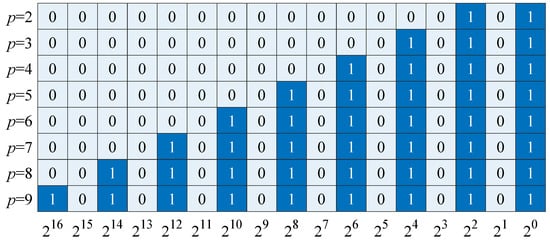
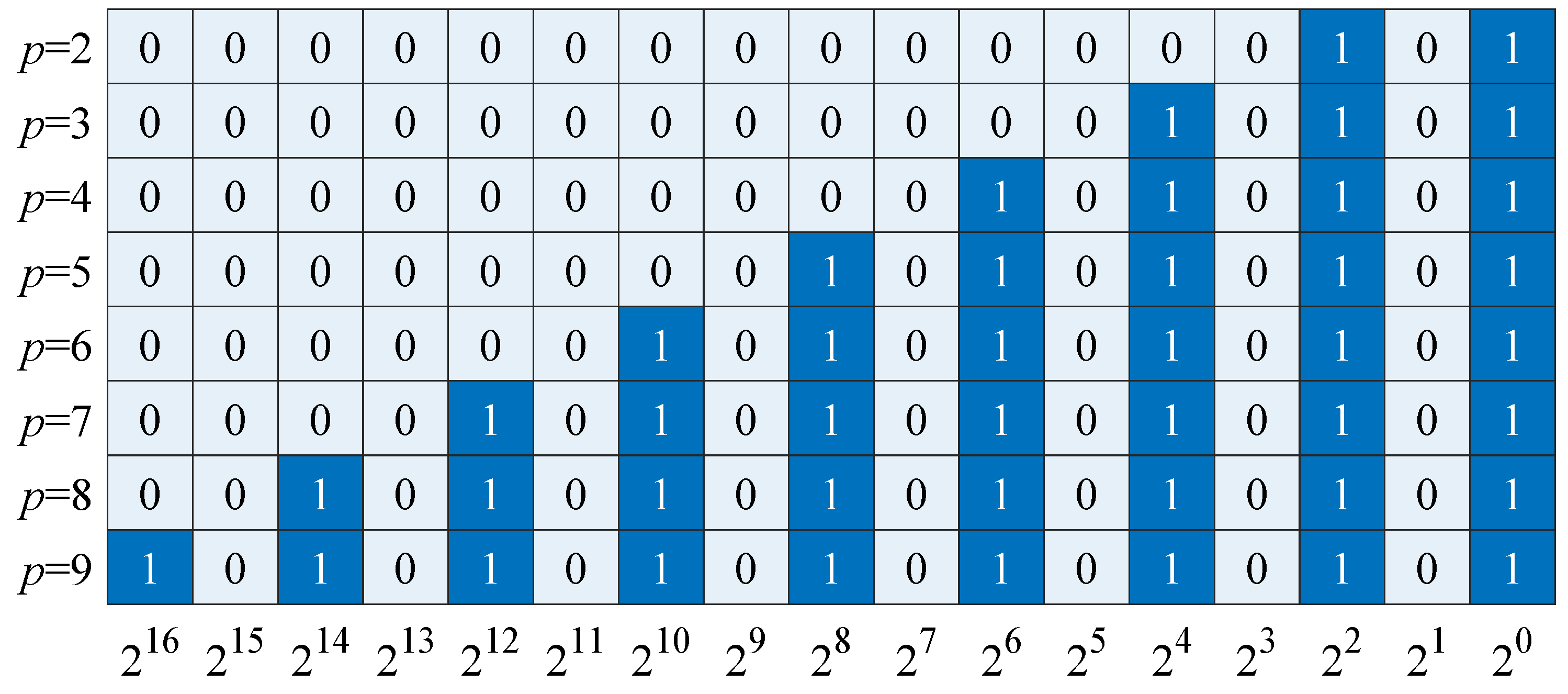
Figure 3 displays self-similarity patterns in the binary representations of the attractors $X^p$, with $p=2,\dots ,9$ shown for illustration. The properties of these basins are analyzed below.

Figure 3. Binary representations of the attractors $X^p=(4^p-1)/3=$ 5, 21, 85, 341, 1365, 5461, 21,845, 87,381 for $p=2,3,\dots ,9$.

Nontrivial Cases ($p\ge 2$)

For $F_2(p,k_1)$, the values $F_2(p,1)$ and $F_2(p,2)$ determine all $F_2(p,k_1)$ through the recursion relation in Equation (15). Representative examples are

$$\begin{array}{cccccc}\hfill F_2(1,1)& ={\displaystyle \frac{1}{3}},\hfill & \hfill F_2(2,1)& =3,\hfill & \hfill F_2(3,1)& ={\displaystyle \frac{41}{3}},\hfill \\ \hfill F_2(1,2)& =1,\hfill & \hfill F_2(2,2)& ={\displaystyle \frac{19}{3}},\hfill & \hfill F_2(3,2)& ={\displaystyle \frac{83}{3}}.\hfill \end{array}$$

(29)

The recursion also implies

$$\left\{\begin{array}{c}{F}_2(p+3,1)=7·2^{2p+1}+F_2(p,1),\hfill \\ F_2(p+3,2)=7·2^{2p+2}+F_2(p,2).\hfill \end{array}\right.$$

(30)

Equations (29) and (30) lead to the following observations.

1.

$F_2(p,k_1)\in \mathbb{O}$ if and only if either $p=2+3m$ and $k_1=2n-1$, or $p=4+3m$ and $k_1=2n$, where $m\in \mathbb{Z}$ and $n\in {\mathbb{Z}}^{+}$.

2.

When $p=3n$, the values $F_2(p,k_1)$ are fractional, which implies that $X_0=X^p$ is the only integer initial value in the basin labeled by $p=3n$.

These conclusions are consistent with the numerical simulations reported in Section 4.

3.3. The Scheme of Like-Bernoulli Shift Map

Let $X_0\in \mathbb{O}$. The Collatz map gives

$$\left\{\begin{array}{c}{X}_1=3X_0+1,\hfill \\ X_2=X_1/2=M^2\left(X_0\right),\hfill \end{array}\right.$$

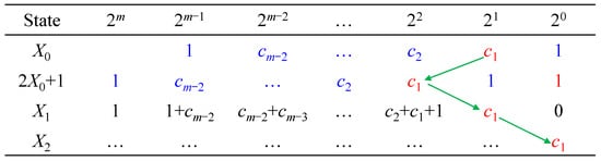
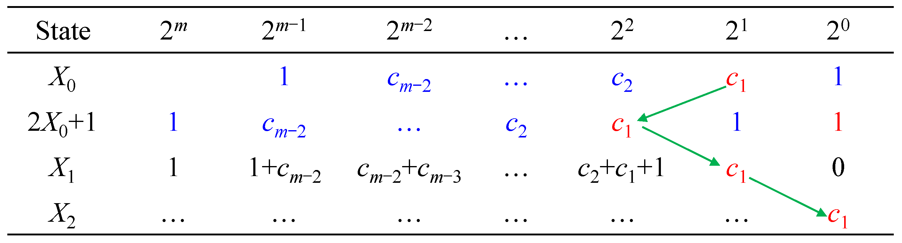
where $X_1$ is necessarily even (see Figure 4). For $2^{m-1}<X_0<2^m$, the binary expansion of $X_0$ can be written as

$$X_0=2^{m-1}+\sum _{j=1}^{m-2}{c}_j{2}^j+2^0,c_j\in \{0,1\},c_0=c_{m-1}=1.$$

Figure 4. Demonstration of iterations in the binary system resembling a Bernoulli shift scheme, where $X_2=M\left(X_1\right)=M^2\left(X_0\right)$, illustrating how the operation $M^2$ moves $c_1$ to the rightmost end.

Figure 4 shows that $2X_0+1$ corresponds to a left shift in binary followed by appending a terminal 1. Moreover, $X_1=X_0+(2X_0+1)$ performs coefficient-wise binary addition. Carry operations occur whenever a digit sum exceeds 1 and then propagate to higher bits. For example, one may write $c_2^{\prime }=(c_2+c_1+1)mod2$ and $c_3^{\prime }=c_3+\lfloor (c_2+c_1+1)/2\rfloor$. This representation highlights a shift-type mechanism: the action of $M^2$ maps the coefficient $c_1$ of $X_0$ to the least significant bit of $X_2$, while the remaining coefficients are updated through addition and carry propagation. The same mechanism applies iteratively to $X_2$ in the subsequent step. When $c_1=1$, the next update again applies $M^2$; when $c_1=0$, the next update applies M. As a consequence, the number of up phases $N_{\uparrow }$ increases by one whenever the $M^2$ branch is taken.

From a statistical viewpoint, the digits $c_j\in \{0,1\}$ may be treated as approximately equiprobable, so the induced dynamics is well approximated by a right-shift process on binary strings. In addition, the ergodicity of the associated binary shift map [47] implies that the binary patterns corresponding to $X^p$ in Figure 3 occur with nonzero frequency along iterative trajectories. These considerations provide theoretical heuristic support for the convergence of the map within the proposed dynamic framework.

Next, numerical experiments will be conducted to investigate the statistical characteristics of the basins of attraction and to validate the theoretical predictions of the iteration count, i.e., the expression (26).

4. Numerical Verifications

Based on the theoretical analysis presented above, only the case where $X_0\in \mathbb{O}$ needs to be considered in the numerical simulations. Since $\mathbb{O}$ contains an infinite number of elements, and statistical analysis can only be performed over a finite interval in practical applications, $X_0$ is restricted to the set $\{3,5,\dots ,2L+1\}$ in specific implementations. Here, L denotes a positive integer that controls the size of the sampling window, and the number of elements falling into the basin of attraction labeled by p is counted simultaneously. The algorithm for the numerical experiments is presented in Appendix A.

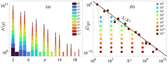
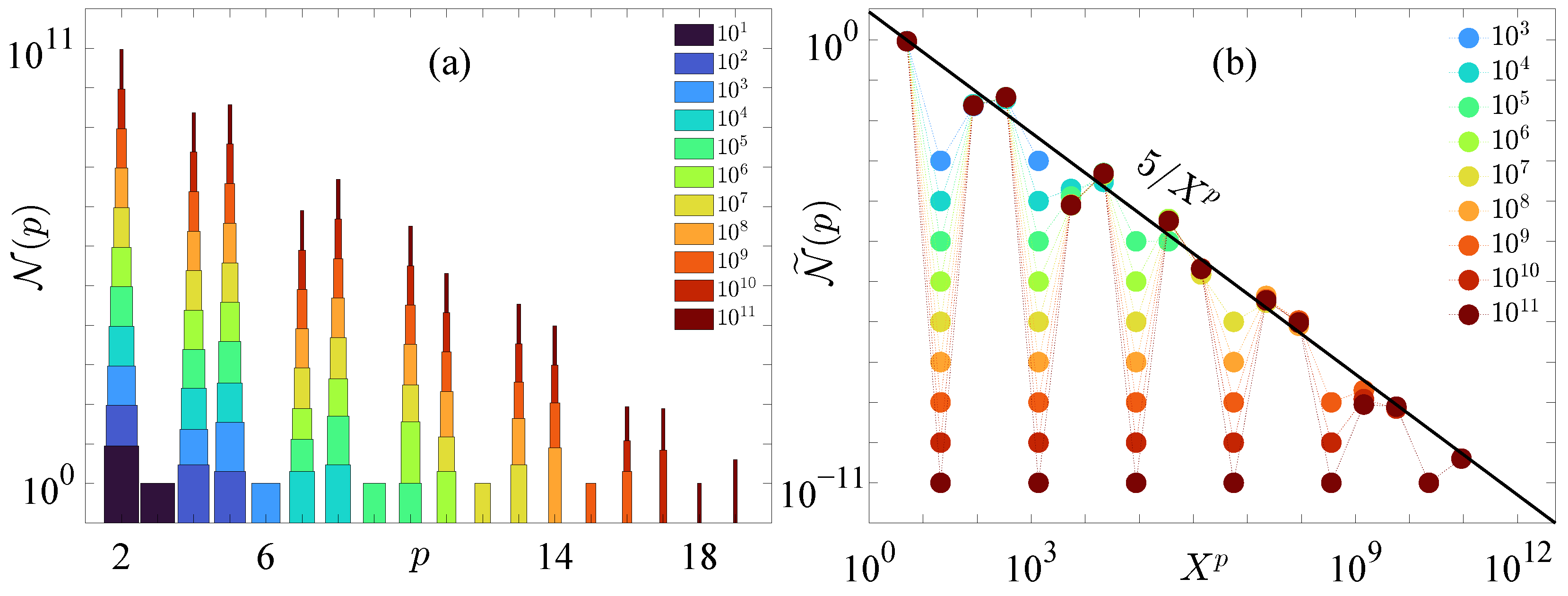
Figure 5a shows the count $\mathcal{N}\left(p\right)$ as a function of p for several values of L. It is observed that $\mathcal{N}\left(2\right)$ is the largest for all tested L. In addition, $\mathcal{N}\left(p\right)=1$ when $\mathrm{mod}(p,3)=0$, consistent with the theoretical analysis in Section 3.2. Figure 5b displays the normalized count $\tilde{\mathcal{N}}\left(p\right)=\mathcal{N}\left(p\right)/L$, which represents the fraction of numbers in each basin. Except for the cases $\mathrm{mod}(p,3)=0$, the data indicate $\tilde{\mathcal{N}}\left(p\right)\propto 1/X^p$, as shown by the black reference line. This suggests that the basin sizes follow a power-law distribution, which is consistent with scale invariance and implies the absence of a characteristic basin-size scale [49]. For large L, the fraction $\tilde{\mathcal{N}}\left(2\right)$ approaches $93.77\%$, as summarized in Table 1. Each column of Table 1 sums to exactly L, which indicates that all odd integers up to $2L+1$ are generated by the family of functions $F_s$ with $p\in [2,19]$ in the reported sampling range.

Figure 5. (a) Histograms of number $\mathcal{N}\left(p\right)$ in different attraction basins p within a given range of $X_0\in \{3,5,\dots ,2L+1\}$. The legend shows the values of $L={10}^1,{10}^2,\dots ,{10}^{11}$. (b) Same as the panel (a) but in normalized form $\tilde{\mathcal{N}}\left(p\right)=\mathcal{N}\left(p\right)/L$ and the horizontal axis is replaced by $X^p=F_1\left(p\right)$. The solid line serves as reference.

Table 1. Statistics of numbers in different attraction basins p for $X_0\in \{3,5,\dots ,2L+1\}$ with $L={10}^1,{10}^2,\dots ,{10}^{11}$. Note that each column sums to exactly L.

p	${10}^1$	${10}^2$	${10}^3$	${10}^4$	${10}^5$	${10}^6$	${10}^7$	${10}^8$	${10}^9$	${10}^{10}$	${10}^{11}$
2	9	94	940	9395	93,679	938,003	9,378,361	93,772,537	937,676,531	9,377,184,614	93,774,783,120
3	1	1	1	1	1	1	1	1	1	1	1
4	0	3	23	255	2412	23,743	237,828	2,373,777	23,761,165	237,454,856	2,373,306,213
5	0	2	35	343	3842	37,687	377,838	3,793,838	37,961,580	379,374,692	3,792,124,912
6	0	0	1	1	1	1	1	1	1	1	1
7	0	0	0	2	13	78	830	8098	80,062	796,409	7,937,609
8	0	0	0	3	50	448	4810	48,229	485,728	4,843,192	48,398,337
9	0	0	0	0	1	1	1	1	1	1	1
10	0	0	0	0	1	36	311	3253	32,329	320,937	3,199,254
11	0	0	0	0	0	2	15	212	2127	20,883	206,700
12	0	0	0	0	0	0	1	1	1	1	1
13	0	0	0	0	0	0	3	44	363	3419	34,128
14	0	0	0	0	0	0	0	8	108	974	9551
15	0	0	0	0	0	0	0	0	1	1	1
16	0	0	0	0	0	0	0	0	2	12	88
17	0	0	0	0	0	0	0	0	0	7	78
18	0	0	0	0	0	0	0	0	0	0	1
19	0	0	0	0	0	0	0	0	0	0	4

In principle, p is unbounded, so the empirical distribution in Table 1 is expected to approach an upper-triangular form as larger values of p become accessible. Resolving nonzero contributions at larger p requires increasing L. Based on the available data, it is conjectured that in the joint limit $p\to \infty$ and $L\to \infty$, the dominant fractions approach $\tilde{\mathcal{N}}\left(2\right)\approx 93.77\%$, $\tilde{\mathcal{N}}\left(4\right)\approx 2.37\%$, and $\tilde{\mathcal{N}}\left(5\right)\approx 3.79\%$. Equivalently, $\tilde{\mathcal{N}}\left(2\right)+\tilde{\mathcal{N}}\left(4\right)+\tilde{\mathcal{N}}\left(5\right)\approx 99.93\%$ remains essentially unchanged, while increasing p and L primarily refines the decimal precision.

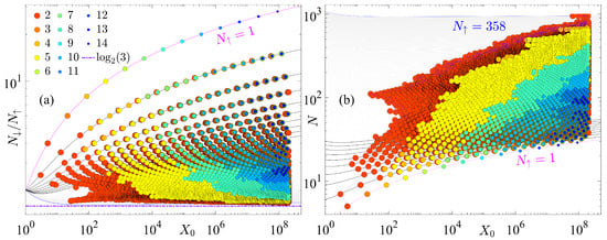
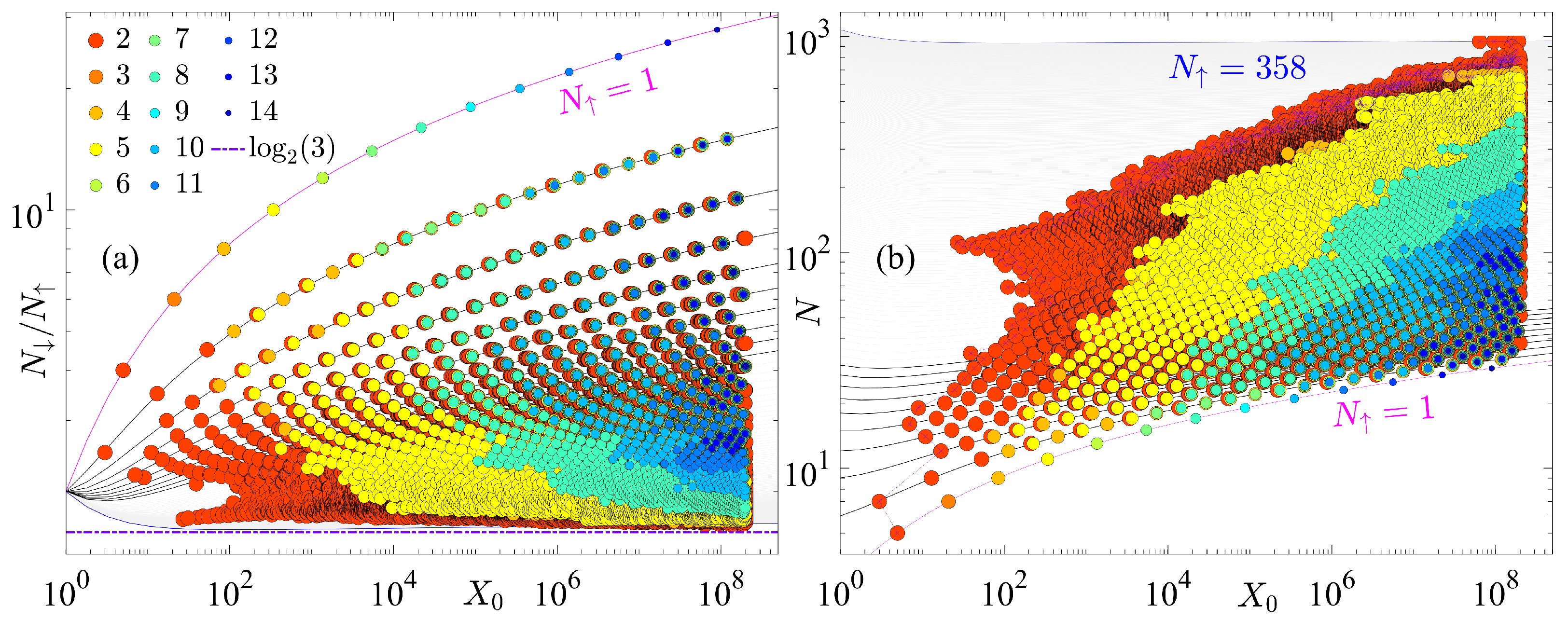
Figure 6a shows the ratio $N_{\downarrow }/N_{\uparrow }$ as a function of $X_0$, where different colors correspond to different attraction basins labeled by p, as indicated in the legend. The solid curves are the theoretical predictions from Equation (26). Excellent agreement between theory and numerics is observed. As $N_{\uparrow }$ increases, the ratio approaches ${log}_2\left(3\right)\approx 1.585$, as indicated by the purple horizontal dashed line. Figure 6b shows the total iteration number N versus $X_0$. The growth of N with $X_0$ is slow, and the numerical results are consistent with the theoretical prediction from Equation (26). This agreement supports the conclusion that the iteration count remains finite relative to $X_0$, consistent with Equations (27) and (28). In Figure 6b, the purple dotted curve with cross markers indicates an upper boundary composed of points having the smallest $X_0$ for a fixed $N_{\uparrow }$. The boundaries separating basins for different p exhibit coastline-like geometry and strong visual similarity. The basin with $p=2$ occupies nearly the entire computed interval, consistent with the statistics in Figure 5. In particular, all points on the upper boundary belong to the basin with $p=2$.

Figure 6. Dependence of $N_{\downarrow }/N_{\uparrow }$ (a) and $N=N_{\downarrow }+N_{\uparrow }$ (b) on $X_0=2n+1$ for $n=1,2,\dots ,{10}^8$. Colors denote attraction basins labeled by p (legend in panel (a) shows the values of p, shared by both panels). Solid lines show the theoretical predictions from Equation (26). The purple crossed dotted curve in panel (b) marks the upper boundary, which is replotted in Figure 7a.

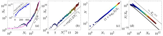
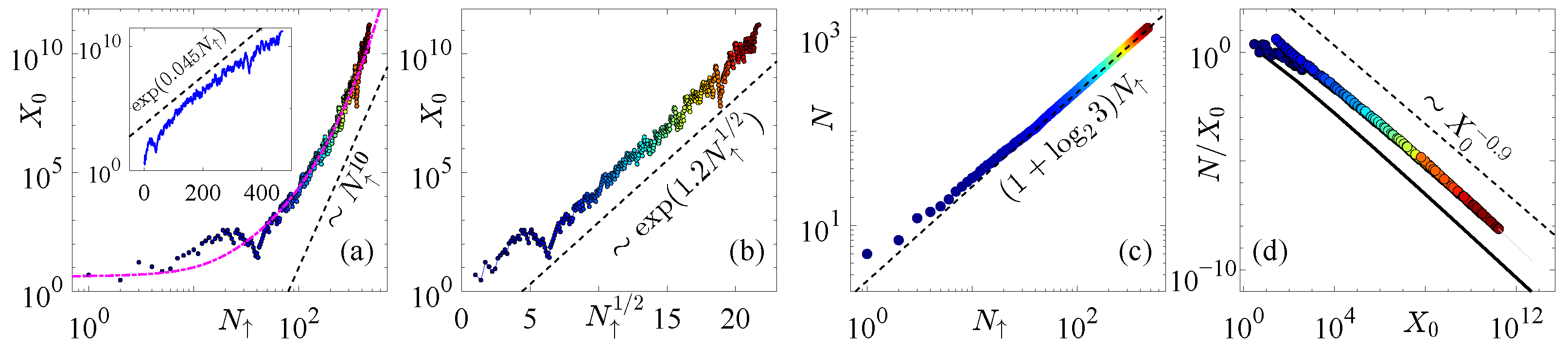
To further characterize the upper-boundary points (see cross markers) in Figure 6b, Figure 7 displays their behavior over a wider range. The abscissa $X_0$ and ordinate N of these boundary points are plotted as functions of $N_{\uparrow }$ in Figure 7a–c. Figure 7a shows that $X_0$ increases approximately in a stretched-exponential manner with $N_{\uparrow }$, as indicated by the magenta dashed curve. This growth is faster than a power law but slower than an exponential, as illustrated by the reference curves and the inset. Figure 7b provides a clearer representation of this trend, with $X_0\propto exp\left(1.2N_{\uparrow }^{1/2}\right)$. The distribution of $X_0$ along the boundary also exhibits a self-similar fractal pattern reminiscent of a coastline. Figure 7c shows N as a function of $N_{\uparrow }$, indicating an approximately linear increase. For large $X_0$, Equation (26) yields $N\approx [1+{log}_2\left(3\right)]N_{\uparrow }$, which agrees well with the numerical results. Figure 7d shows $N/X_0$ as a function of $X_0$, where the black curve is the theoretical prediction derived from Equation (26). The ratio $N/X_0$ decreases toward zero as $X_0\to \infty$, indicating that the iteration count becomes negligible relative to large $X_0$.

Figure 7. (a) $X_0$ of the upper-boundary points (extracted from Figure 6b) as a function of $N_{\uparrow }$ in log–log scale. The magenta dashed curve shows the stretched-exponential fit $exp\left(1.2N_{\uparrow }^{1/2}\right)/7+4$; inset: the same data in semi-log scale. (b) The same data as in panel (a) with the abscissa rescaled to $N_{\uparrow }^{1/2}$. (c) Total iteration count $N=N_{\uparrow }+N_{\downarrow }$ versus $N_{\uparrow }$ for the same boundary points. (d) Ratio $N/X_0$ versus $X_0$ for the same data; the black curve is the prediction from Equation (26) with $N_{\uparrow }=1$. Dashed lines in all panels serve as references.

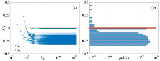
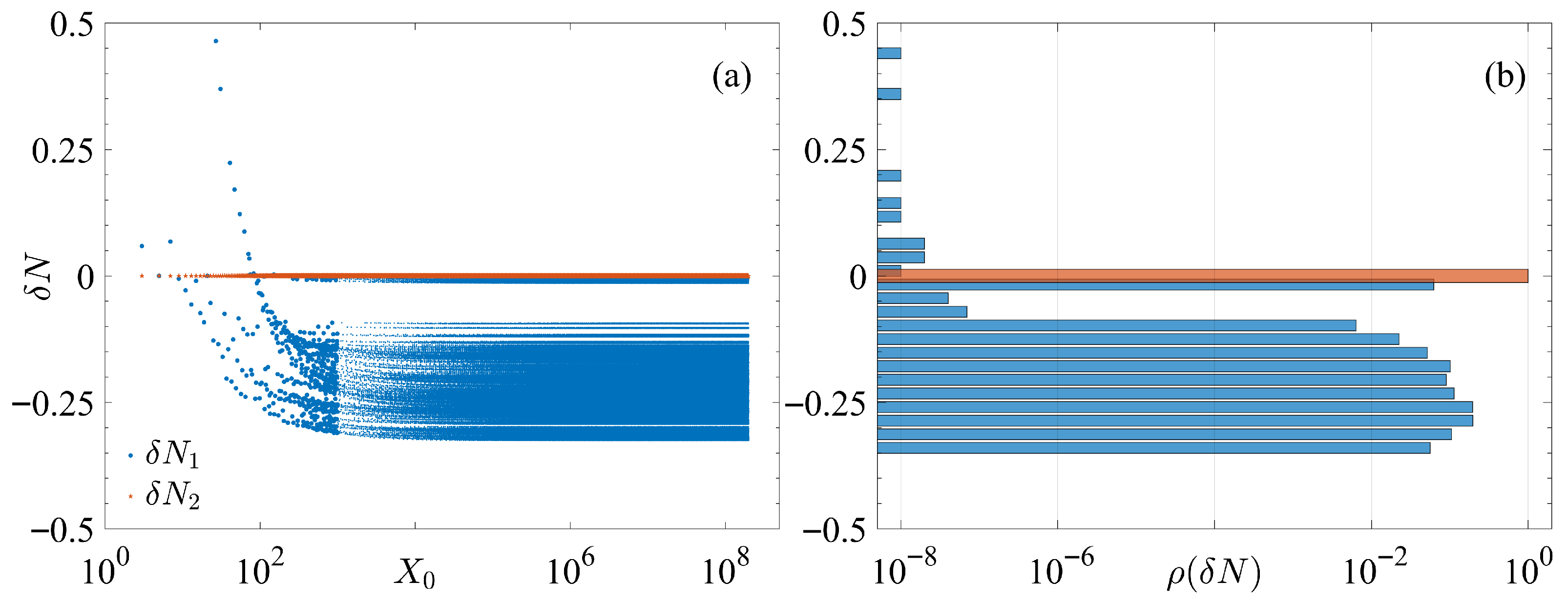
To further quantify the gap between the theoretically estimated iteration count (see Equation (26)) and the numerically obtained iteration count, Figure 8a shows the magnitude of this deviation for $X_0\in \{3,5,\dots ,2\times {10}^8+1\}$. Specifically, the difference $\delta N$ between the theoretical values and the actual iteration numbers N is displayed. The blue dots represent the differences before rounding, i.e., $\delta N_1=s\left[1+{log}_2\left(3+{\displaystyle \frac{1}{X_0}}\right)\right]+{log}_2\left(X_0\right)-N$, while the orange stars show the differences after rounding, i.e., $\delta N_2=N_s-N$. It is observed that $-0.35<\delta N_1<0.5$ and $\delta N_2=0$ within the tested range. Figure 8b presents the statistical distribution of $\delta N$ corresponding to panel (a), where the horizontal axis represents the proportion of data points within each statistical interval, while the vertical axis is the same as in panel (a). It is evident that $-0.35<\delta N_1<0.025$ for $X_0>{10}^2$, while $\rho (\delta N_2=0)=1$ for all $X_0$. This confirms that the theoretical estimation aligns perfectly with the experimental results.

Figure 8. (a) The difference $\delta N$ between the theoretical values (see Equation (26)) and the actual iteration numbers N for convergence with initial value $X_0=2n+1$ for $n=1,2,\dots ,{10}^8$. The blue dots represent the differences before rounding, i.e., $\delta N_1=s\left[1+{log}_2\left(3+1/X_0\right)\right]+{log}_2\left(X_0\right)-N$, while the orange stars show the differences after rounding, i.e., $\delta N_2=N_s-N$. For clarity, blue dots for $X_0<1000$ are shown in a larger size. (b) The statistical distribution of $\delta N$ corresponding to panel (a), where the horizontal axis represents the proportion of data points within each statistical interval.

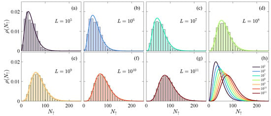
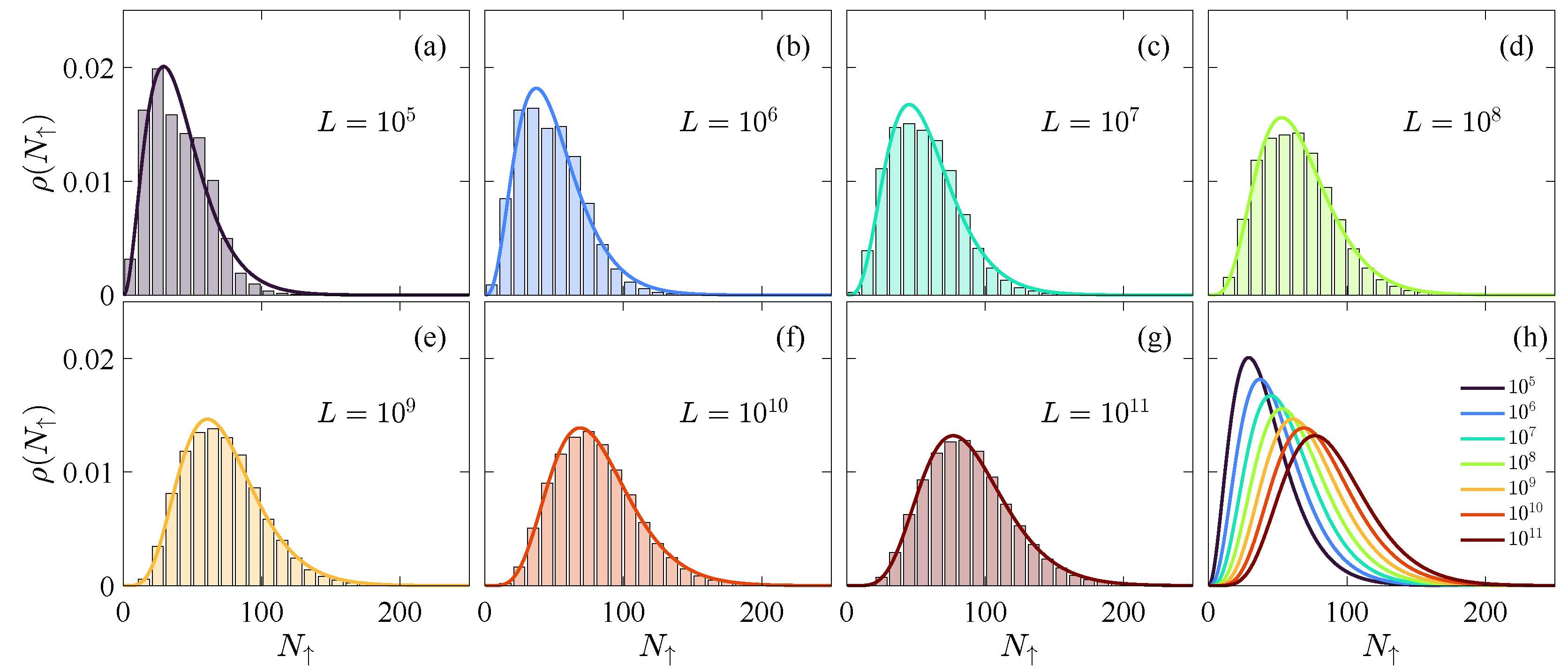
Figure 9 shows the distribution of $N_{\uparrow }$ for the sampling window $X_0\in \{3,5,\dots ,2L+1\}$. The histogram height gives the fraction of initial values sharing the same $N_{\uparrow }$. As shown in Figure 9a–g, the data are well approximated by a Gamma distribution of the form $\rho \left(x\right)={\displaystyle \frac{A}{{\theta }^K\Gamma \left(K\right)}}{x}^{K-1}{e}^{-x/\theta }$, as indicated by the solid curves. Equation (21) suggests a possible analytical route toward explaining the emergence of Gamma statistics, and developing this theoretical basis is left for future work. The distribution becomes broader as L increases, as summarized by the fitted curves in Figure 9h.

Figure 9. (a–g) The distribution of numbers over $N_{\uparrow }$ within a given interval of $X_0\in [3,5,\dots ,2L+1]$. The solid line is a fitting curve based on the Gamma distribution with the form of $\rho \left(x\right)={\displaystyle \frac{A}{\Gamma \left(K\right){\theta }^K}}{x}^{K-1}{e}^{-x/\theta }$. (h) Summarization of all fitted curves together for comparison.

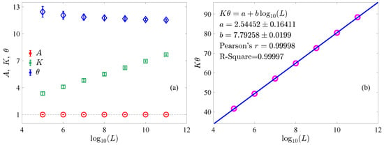
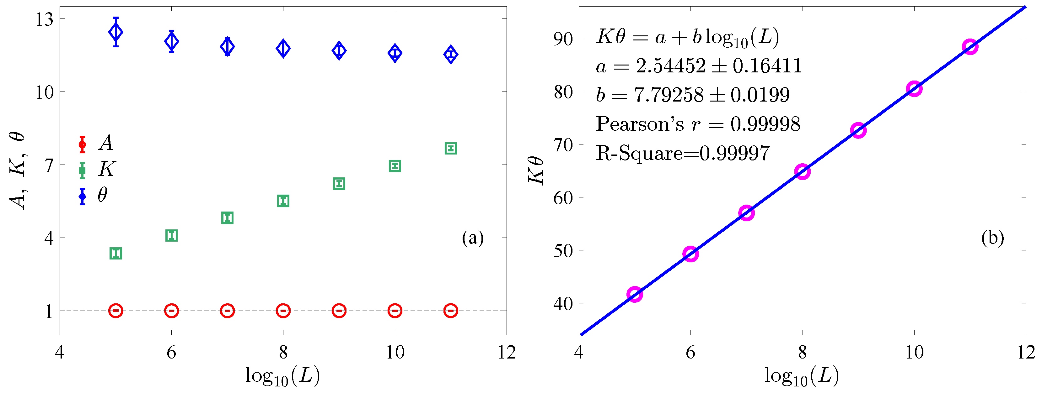
Figure 10a displays the dependence of the Gamma parameters on L. The normalization parameter remains close to unity, with $A\simeq 1$. The shape parameter K increases with L and is approximately proportional to ${log}_{10}\left(L\right)$, whereas the scale parameter $\theta$ exhibits a weak decreasing trend and stays nearly constant over the explored range. The mean of the Gamma distribution, ${\overline{N}}_{\uparrow }=K\theta$, increases with L, as shown in Figure 10b. A linear fit yields ${\overline{N}}_{\uparrow }\approx 2.54+7.79{log}_{10}\left(L\right)$.

Figure 10. (a) The fitting parameters of the Gamma distribution function in Figure 9 as a function of L. (b) Dependence of the mean value of the Gamma distribution $K\theta$ on L.

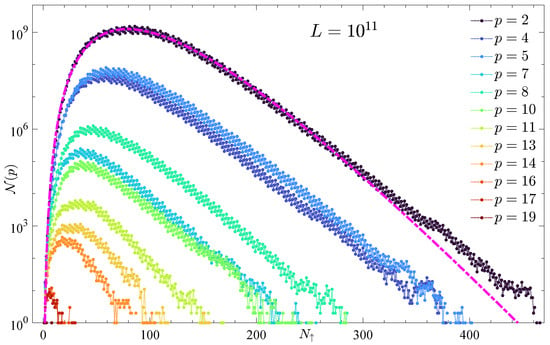
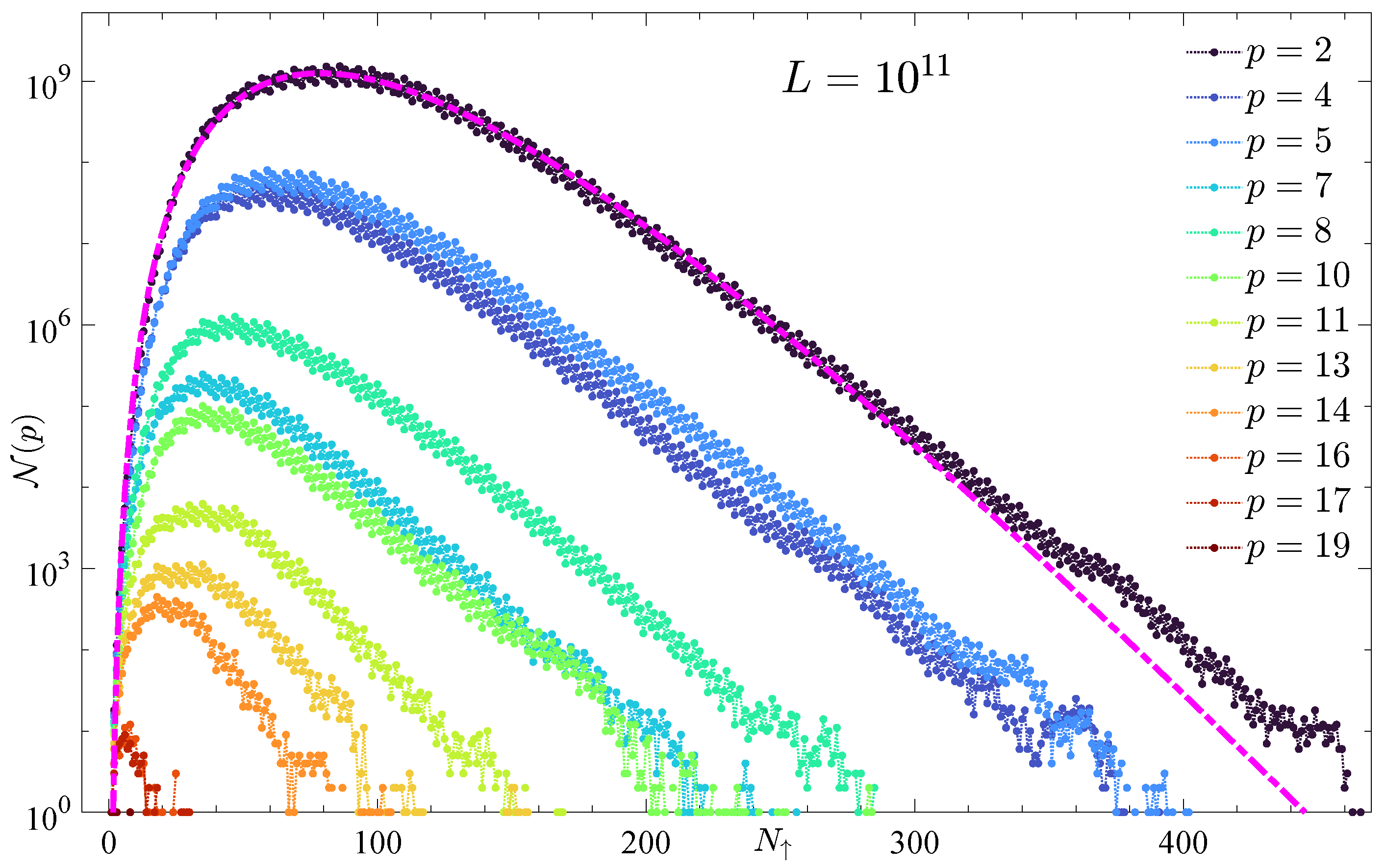
In addition, the distribution of $N_{\uparrow }$ is counted by the attraction basin within the range $X_0\in \{3,5,\dots ,2L+1\}$ by fixing $L={10}^{11}$. The results are shown in Figure 11, where $\mathcal{N}\left(p\right)$ denotes the number of initial values in basin p. Each $\mathcal{N}\left(p\right)$ is well described by a Gamma distribution with basin-dependent parameters. For $p=2$, the fitted curve nearly overlaps the data points, as indicated by the magenta dashed curve.

Figure 11. The count number $\mathcal{N}\left(p\right)$ over $N_{\uparrow }$ within a given interval of $X_0\in [3,5,\dots ,2L+1]$ in a semi-log scale. The magenta dashed line is a fitting curve based on the Gamma distribution.

5. Summary and Discussions

In summary, the Collatz map is studied from a nonlinear-dynamics viewpoint, focusing on the structure of its iterative orbits. Four principal outcomes are obtained. First, arranging positive integers via Sharkovsky’s ordering shows that restricting analysis to odd initial values suffices for a dynamical characterization. Second, a classification scheme based on “direction phases” is introduced to partition iterations into ascending and descending segments. Within this scheme, a logarithmic scaling relation between the iteration count and the initial value is derived from the recursive family $F_s$ parameterized by the up-phase number s—see Equation (19)—which establishes finite-time convergence to the period-three cycle for $X_0\in \mathbb{F}$. Third, a dynamical equivalence between the Collatz map and a binary shift map is identified, and the ergodic properties of the shift map provide further theoretical support for convergence. Fourth, numerical simulations reveal that attraction basins follow power-law statistics and display marked self-similarity (see Figure 3, Figure 6 and Figure 11), and that odd integers grouped by up-phase counts are well described by Gamma distributions.

Beyond its theoretical relevance, the framework may be relevant to applications in which discrete nonlinear maps and symbolic dynamics are central. The equivalence between the Collatz map and a binary shift map, together with the ergodic and self-similar features of the basin structure, suggests potential utility in cryptographic constructions, pseudorandom number generation, and complexity-based hashing, where strong mixing properties and scale-free organization are desirable. The power-law basin statistics and the Gamma-type fluctuations in up-phase counts further indicate that Collatz dynamics naturally produces broad distributions, which may be useful for stochastic modeling and the design of randomized algorithms. In addition, recasting a classical number-theoretic problem as a visualizable and computable nonlinear dynamical model provides an instructive case study for undergraduate and graduate teaching, clarifying the connections among symbolic dynamics, ergodicity, scaling laws, and discrete maps.

Several directions for future research follow naturally. Within the tested computational range, all sampled odd integers are consistent with an $F_s$ representation, supporting the hypothesis that every odd integer admits a parametrization of the form $F_s$. Proving this statement rigorously would verify the completeness condition $\mathbb{O}\equiv \mathbb{F}$ and thereby resolve the Collatz conjecture. The structural properties of $F_s$ may also connect to broader questions in number theory, since all primes other than 2 belong to the conjectured $F_s$ generated subset of odd integers. Another important problem is to develop theoretical estimates or bounds for the up-phase number s associated with a given initial value $X_0$. In addition, an analytical explanation for the observed Gamma statistics remains open and may be approached by analyzing Equation (21) and its underlying combinatorial structure. More broadly, extensions to generalized $3X+1$ type maps, stochastic perturbations, and higher-dimensional symbolic representations may clarify the robustness and universality of the reported scaling laws and basin geometry. Finally, algorithmic and cryptographic developments that exploit the shift-map representation and the basin hierarchy may reveal practical uses of Collatz-type dynamics beyond pure number theory.

Appendix A.1. Parameters and Data Structures

It should be noted that for a given large $L_{max}$, both $P_{max}$ and $S_{max}$ need to take large values to avoid the risk of array (or matrix) index out-of-bounds errors. Of course, an allocatable array (or matrix) could also be used to avoid this risk, but the algorithm presented below uses a fixed array (or matrix). See Table A1.

Table A1. Algorithm parameters and data structures.

Name	Type	Description
$S_{max}$	Integer parameter	Maximum number of upward phases tracked in distribution
$P_{max}$	Integer parameter	Number of target attractor categories
$L_{max}$	Integer parameter	Maximum exponent of the power function with base 10
$counts\left[p\right]\left[s\right]$	Integer matrix	Number of sequences for attractor p with s up-phases
$clist\left[p\right]$	Integer array	Total count of sequences ending with attractor value $list\left[p\right]$ for $p=1,\dots ,P_{max}$
$list\left[p\right]$	Integer array	Target attractor values: $list\left[p\right]=(4^p-1)/3$
$m\left[k\right]$	Integer array	Milestone thresholds: $m\left[k\right]={10}^k$ for $k=1,\dots ,L_{max}$

Table A1. Algorithm parameters and data structures.

Name	Type	Description
$S_{max}$	Integer parameter	Maximum number of upward phases tracked in distribution
$P_{max}$	Integer parameter	Number of target attractor categories
$L_{max}$	Integer parameter	Maximum exponent of the power function with base 10
$counts\left[p\right]\left[s\right]$	Integer matrix	Number of sequences for attractor p with s up-phases
$clist\left[p\right]$	Integer array	Total count of sequences ending with attractor value $list\left[p\right]$ for $p=1,\dots ,P_{max}$
$list\left[p\right]$	Integer array	Target attractor values: $list\left[p\right]=(4^p-1)/3$
$m\left[k\right]$	Integer array	Milestone thresholds: $m\left[k\right]={10}^k$ for $k=1,\dots ,L_{max}$

Appendix A.2. Output Files

1_Counts_X0.txt: Record the number of iterations and the number of upward phases corresponding to the initial value $X_0$.

At each milestone $m\left[k\right]={10}^k$, the algorithm generates:

• 2_Distr_num_up_1Ek.txt: Distribution matrix showing $counts\left[p\right]\left[s\right]$ for all p, s.
• 3_Distr_door_1Ek.txt: Summary showing $clist\left[p\right]$ for each attractor category p.

Appendix A.3. Algorithm

Algorithm A1: Collatz Statistical Analysis

Require:    1: Initialize $S_{max}=600$, $P_{max}=25$, $L_{max}=11$ 2: Initialize $counts\left[P_{max}\right]\left[S_{max}\right]\leftarrow 0$                                                        ▷ Distribution matrix 3: Initialize $clist\left[P_{max}\right]\leftarrow 0$                                                 ▷ Count for each attractor category 4: Initialize $m\left[L_{max}\right]$                                                                                  ▷ Milestone thresholds 5: for $k\leftarrow 1$ to $L_{max}$ do 6:     $m\left[k\right]\leftarrow {10}^k$                                                                              ▷ Milestone: ${10}^1,{10}^2,{10}^3,\dots$ 7: end for 8: for $p\leftarrow 1$ to $P_{max}$ do 9:     $list\left[p\right]\leftarrow (4^p-1)/3$                                                               ▷ Target values of attractors 10: end for 11: $n\leftarrow 0$ 12: for $k\leftarrow 1$ to $L_{max}$ do                                                                        ▷ Process each milestone 13:     while $n<m\left[k\right]$ do 14:         $n\leftarrow n+1$                                                                                      ▷ Increment n counter 15:         $X_0\leftarrow 2\times n+1$                                                                               ▷ Odd starting value 16:         $X\leftarrow X_0$                                                                                                    ▷ Starting value 17:         $N\leftarrow 0$                                                                   ▷ Reset the counter of total iterations 18:         $s\leftarrow 0$                                                                           ▷ Reset the counter for up-phases 19:         while $X>1$ do                                                                                   ▷ Collatz iteration 20:            if $Xmod2=1$ then 21:                $attractor\leftarrow X$                                               ▷ Record last odd value, i.e., attractor 22:            end if 23:            $X\leftarrow \mathrm{CollatzStep}(X,s)$                                       ▷ Update X and s by Algorithm A2 24:            $N\leftarrow N+1$                                                                                    ▷ Increment counter 25:         end while 26:         for $p\leftarrow 1$ to $P_{max}$ do                                                    ▷ Categorize by attractor value 27:            if $attractor=list\left[p\right]$ then 28:                $clist\left[p\right]\leftarrow clist\left[p\right]+1$                                            ▷ Only classified by attractors 29:                $counts\left[p\right]\left[s\right]\leftarrow counts\left[p\right]\left[s\right]+1$        ▷ Classified by attractors and up-phases 30:                break 31:            end if 32:         end for 33:         Write $X_0$, N, and s into the file 1_Counts_X0.txt                           ▷ Output results 34:     end while 35:     Write $counts$ into 2_Distr_num_up_1Ek.txt      ▷ Output results for milestone $m\left[k\right]$ 36:     Write $clist$ into 3_Distr_door_1Ek.txt 37: end for

Algorithm A2: CollatzStep$(X,s)$                                      ▷ Apply Collatz transformation rule

1: if  $Xmod2=0$then 2:     return $X/2$ 3: else 4:     $s\leftarrow s+1$                                                                                  ▷ Increment “3X+1” counter 5:     return $3X+1$ 6: end if

References

- Ott, E. Strange attractors and chaotic motions of dynamical systems. Rev. Mod. Phys. 1981, 53, 655–671. [Google Scholar] [CrossRef] [Scilit]
- Kozak, J.J.; Musho, M.K.; Hatlee, M.D. Chaos, Periodic Chaos, and the Random-Walk Problem. Phys. Rev. Lett. 1982, 49, 1801–1804. [Google Scholar] [CrossRef] [Scilit]
- Mogavero, F.; Hoang, N.H.; Laskar, J. Timescales of Chaos in the Inner Solar System: Lyapunov Spectrum and Quasi-integrals of Motion. Phys. Rev. X 2023, 13, 021018. [Google Scholar] [CrossRef] [Scilit]
- Pazó, D. Discontinuous transition to chaos in a canonical random neural network. Phys. Rev. E 2024, 110, 014201. [Google Scholar] [CrossRef] [Scilit]
- Börner, S.D.; Berke, C.; DiVincenzo, D.P.; Trebst, S.; Altland, A. Classical chaos in quantum computers. Phys. Rev. Res. 2024, 6, 033128. [Google Scholar] [CrossRef] [Scilit]
- Lippolis, D. Thermodynamics of chaotic relaxation processes. Phys. Rev. E 2024, 110, 024215. [Google Scholar] [CrossRef] [Scilit] [PubMed]
- Fuchs, A. Nonlinear Dynamics in Complex Systems; Springer: Berlin/Heidelberg, Germany, 2014. [Google Scholar] [CrossRef] [Scilit]
- Abraham, R.H.; Gardini, L.; Mira, C. Chaos in Discrete Dynamical Systems, 1st ed.; Springer: New York, NY, USA, 1997. [Google Scholar] [CrossRef] [Scilit]
- Peitgen, H.O.; Jürgens, H.; Saupe, D. Chaos and Fractals: New Frontiers of Science, 2nd ed.; Springer: Berlin/Heidelberg, Germany, 2004. [Google Scholar]
- Yao, K.E.; Shi, Y. Hopf bifurcation in three-dimensional based on chaos entanglement function. Chaos Solitons Fractals X 2019, 4, 100027. [Google Scholar] [CrossRef] [Scilit]
- Rouah, H. Stability analysis and suppress chaos in the generalized Lorenz model. Chaos Solitons Fractals X 2024, 12, 100104. [Google Scholar] [CrossRef] [Scilit]
- Feigenbaum, M.J. Quantitative universality for a class of nonlinear transformations. J. Stat. Phys. 1978, 19, 25–52. [Google Scholar] [CrossRef] [Scilit]
- Chirikov, B.V. A universal instability of many-dimensional oscillator systems. Phys. Rep. 1979, 52, 263–379. [Google Scholar] [CrossRef] [Scilit]
- Ott, E. Chaos in Dynamical Systems, 2nd ed.; Cambridge University Press: Cambridge, UK, 2002. [Google Scholar]
- Mackey, M.C. The dynamic origin of increasing entropy. Rev. Mod. Phys. 1989, 61, 981–1015. [Google Scholar] [CrossRef] [Scilit]
- Driebe, D.J. Volume 4: Nonlinear Phenomena and Complex Systems. In Fully Chaotic Maps and Broken Time Symmetry; Springer: Dordrecht, The Netherlands, 1999. [Google Scholar] [CrossRef] [Scilit]
- Li, C.; Tan, K.; Feng, B.; Lü, J. The Graph Structure of the Generalized Discrete Arnold’s Cat Map. IEEE Trans. Comput. 2022, 71, 364–377. [Google Scholar] [CrossRef] [Scilit]
- Oliveira, J.A.; Brochero Martínez, F.E. Dynamics of polynomial maps over finite fields. Des. Codes Cryptogr. 2024, 92, 1113–1125. [Google Scholar] [CrossRef] [Scilit]
- Li, C.; Lu, X.; Tan, K.; Chen, G. Graph Structure of Chebyshev Permutation Polynomials Over Ring . IEEE Trans. Inf. Theory 2025, 71, 1419–1433. [Google Scholar] [CrossRef] [Scilit]
- Ghosh, I.; McLachlan, R.I.; Simpson, D.J. The bifurcation structure within robust chaos for two-dimensional piecewise-linear maps. Commun. Nonlinear Sci. 2024, 134, 108025. [Google Scholar] [CrossRef] [Scilit]
- Méndez-Bermúdez, J.; Aguilar-Sánchez, R. Tunable subdiffusion in the Caputo fractional standard map. Commun. Nonlinear Sci. 2024, 135, 108075. [Google Scholar] [CrossRef] [Scilit]
- Borges, V.S.; Silva, M.T.; Eisencraft, M. Chaotic properties of an FIR filtered Hénon map. Commun. Nonlinear Sci. 2024, 131, 107845. [Google Scholar] [CrossRef] [Scilit]
- Meiss, J.; Sander, E. Resonance and weak chaos in quasiperiodically-forced circle maps. Commun. Nonlinear Sci. 2025, 142, 108562. [Google Scholar] [CrossRef] [Scilit]
- Šharkowskii, A.N. Co-existence of the cycles of a continuous mapping of the line into itself. Ukrain. Mat. Z. 1964, 16, 61–71. [Google Scholar]
- Štefan, P. A theorem of Šarkovskii on the Existence of Periodic Orbits of Continuous Endomorphisms of the Real Line. Commun. Math. Phys. 1977, 54, 237–248. [Google Scholar] [CrossRef] [Scilit]
- Li, T.Y.; Yorke, J.A. Period Three Implies Chaos. Amer. Math. Mon. 1975, 82, 985–992. [Google Scholar] [CrossRef] [Scilit]
- Kloeden, P.E. On Sharkovsky’s cycle coexistence ordering. Bull. Aust. Math. Soc. 1979, 20, 171–177. [Google Scholar] [CrossRef] [Scilit]
- Oestreicher, C. A history of chaos theory. Dialogues Clin. Neuro. 2007, 9, 279–289. [Google Scholar] [CrossRef] [Scilit]
- Lorenz, E.N. Deterministic nonperiodic flow. J. Atmos. Sci. 1963, 20, 130–141. [Google Scholar] [CrossRef] [Scilit]
- Prigogine, I.; Stengers, I. The End of Certainty; Simon and Schuster: New York, NY, USA, 1997. [Google Scholar]
- Zaslavsky, G.M. Hamiltonian Chaos and Fractional Dynamics; Oxford University Press: New York, NY, USA, 2005. [Google Scholar]
- Gleick, J. Chaos: Making a New Science; Penguin: London, UK, 2008. [Google Scholar]
- Sinai, Y.G. Statistical (3x + 1) problem. Commun. Pure Appl. Math. 2003, 56, 1016–1028. [Google Scholar] [CrossRef] [Scilit]
- Wirsching, G.J. The Dynamical System Generated by the 3n+1 Function, 1st ed.; Lecture Notes in Mathematics; Springer: Berlin/Heidelberg, Germany, 1998; Volume 1681. [Google Scholar] [CrossRef] [Scilit]
- Lagarias, J.C. The 3x + 1 Problem and its Generalizations. Amer. Math. Mon. 1985, 92, 3–23. [Google Scholar] [CrossRef] [Scilit]
- Lagarias, J.C. The 3x+1 problem: An annotated bibliography (1963–1999) (sorted by author). arXiv 2011, arXiv:math/0309224. [Google Scholar] [CrossRef] [Scilit]
- Lagarias, J.C. The 3x+1 Problem: An Annotated Bibliography, II (2000–2009). arXiv 2012, arXiv:math/0608208. [Google Scholar] [CrossRef] [Scilit]
- Lagarias, J.C. The 3x+1 Problem: An Overview. arXiv 2021, arXiv:2111.02635. [Google Scholar] [CrossRef] [Scilit]
- Hu, Z. The Analysis of Convergence for the 3X + 1 Problem and Crandall Conjecture for the aX + 1 Problem. Adv. Pure Math. 2021, 11, 400–407. [Google Scholar] [CrossRef]
- Tao, T. Almost all orbits of the Collatz map attain almost bounded values. Forum Math. Pi 2022, 10, e12. [Google Scholar] [CrossRef] [Scilit]
- Wang, M.; Yang, Y.; He, Z.; Wang, M. The Proof of the 3X + 1 Conjecture. Adv. Pure Math. 2022, 12, 10–28. [Google Scholar] [CrossRef]
- Crandall, R.E. On the “3x + 1 ” Problem. Math. Comput. 1978, 32, 1281–1292. [Google Scholar] [CrossRef] [Scilit]
- Krasikov, I. How Many Numbers Satisfy The 3x + 1 Conjecture? Int. J. Math. Math. Sci. 1989, 12, 791–796. [Google Scholar] [CrossRef] [Scilit]
- Polli, J.G.; Raposo, E.P.; Viswanathan, G.M.; da Luz, M.G.E. Stochastic-like characteristics of arithmetic dynamical systems: The Collatz hailstone sequences. J. Phys. Complex. 2024, 5, 015011. [Google Scholar] [CrossRef] [Scilit]
- Barina, D. Convergence verification of the Collatz problem. J. Supercomput. 2021, 77, 2681–2688. [Google Scholar] [CrossRef] [Scilit]
- Barina, D. Improved verification limit for the convergence of the Collatz conjecture. J. Supercomput. 2025, 81, 810. [Google Scholar] [CrossRef] [Scilit]
- Einsiedler, M.; Ward, T. Ergodic Theory: With a View Towards Number Theory, 1st ed.; Graduate Texts in Mathematics; Springer: London, UK, 2011; Volume 259. [Google Scholar] [CrossRef] [Scilit]
- Wang, W.; Liu, Z.; Hu, B. Phase Order in Chaotic Maps and in Coupled Map Lattices. Phys. Rev. Lett. 2000, 84, 2610–2613. [Google Scholar] [CrossRef] [Scilit] [PubMed]
- Sethna, J.P. Power laws in physics. Nat. Rev. Phys. 2022, 4, 501–503. [Google Scholar] [CrossRef] [Scilit]
Disclaimer/Publisher’s Note: The statements, opinions and data contained in all publications are solely those of the individual author(s) and contributor(s) and not of MDPI and/or the editor(s). MDPI and/or the editor(s) disclaim responsibility for any injury to people or property resulting from any ideas, methods, instructions or products referred to in the content. |
© 2026 by the authors. Licensee MDPI, Basel, Switzerland. This article is an open access article distributed under the terms and conditions of the Creative Commons Attribution (CC BY) license.