Research on Scheduling of Metal Structural Part Blanking Workshop with Feeding Constraints

Abstract

Taking a metal structural part blanking workshop as the application background, this study addresses the challenges of high material variety, long crane feeding travel caused by heterogeneous line-side storage layouts, and frequent machine stoppages due to the limited feeding capacity of a single overhead crane. To this end, an integrated machine–crane dual-resource scheduling model is developed by explicitly considering line-side storage locations. The objective is to minimize the maximum waiting time among all machine tools. Under constraints of material assignment, processing sequence, and the crane’s single-task execution and travel requirements, the storage positions of materials in line-side buffers are jointly optimized. To solve the problem, a genetic algorithm with fitness-value-based crossover is proposed, and a simulated-annealing acceptance criterion is embedded to suppress premature convergence and enhance the ability to escape local optima. Comparative experiments on randomly generated instances show that the proposed algorithm can significantly reduce the maximum waiting time and yield more stable results for medium- and large-scale cases. Furthermore, a simulation based on real production data from an industrial enterprise verifies that, under limited feeding capacity, the proposed method effectively shortens material-waiting time, improves equipment utilization, and enhances production efficiency, demonstrating its effectiveness.

1. Introduction

Metal structural parts constitute key components in a wide range of equipment, including aircraft and spacecraft, ships, automobiles, and power-transmission towers. Their manufacturing process typically comprises overhead-crane feeding, machining, and the transfer of semi-finished products. In blanking workshops, raw materials are usually long tubes (approximately 4–10 m) produced in large quantities and variants, which are subsequently processed on machine tools through operations such as punching and drilling.

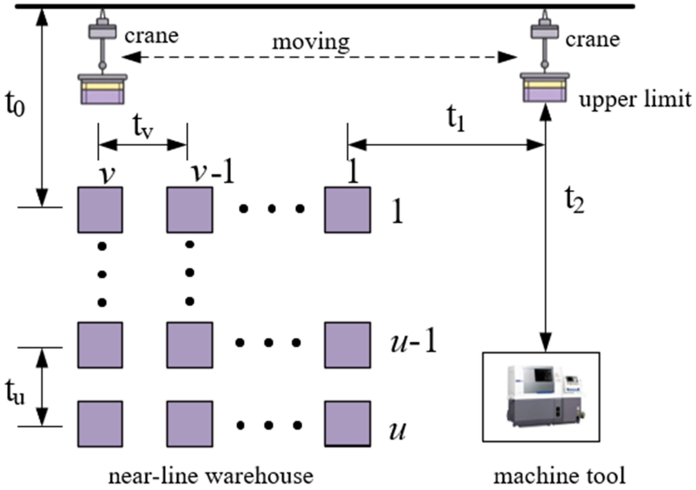
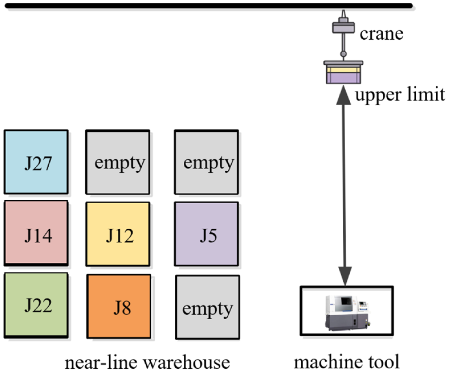
A metal structural parts’ blanking workshop typically consists of multiple parallel machine tools, dedicated line-side buffers for each machine, and a single overhead crane feeding system. The raw materials are mainly standard-length stocks such as tubes, which are transformed into workpieces after blanking operations on the machines, including punching and drilling. During production, when a machine is ready to process the next material batch but the target material is not directly retrievable from the top layer of the corresponding line-side buffer, the crane must first perform a rearrangement operation to bring the target material to an accessible position, and then pick and deliver it to the machine. Consequently, the feeding time is determined not only by the crane travel distance but also by the internal storage level of materials in the line-side buffer and the required rearrangement operations.

The feeding-constrained scheduling problem in a metal structural parts’ blanking workshop involves coupled decisions because a single overhead crane serves multiple machines and can execute only one feeding task at a time. It therefore jointly determines the material-to-machine assignment together with the corresponding processing sequence, the execution order of crane feeding tasks, and the storage locations with stacking order in line-side buffers, aiming to reduce machine idle time and downtime caused by feeding delays. From the perspectives of processing, feeding, transportation, and inventory and storage location, existing studies in the literature can be broadly classified into the following categories.

(1) 

Integrated Scheduling of Processing and Transportation Resources with Automated Guided Vehicles (AGVs) or Robots

Wang et al. [1] investigated the coordination between a flexible flow shop and AGV transportation, and proposed an integrated production–transportation scheduling framework, denoted as FFSPAGV. A mixed-integer linear programming model was developed to jointly represent production constraints and AGV task conflicts, aiming to improve makespan and overall system efficiency. Zhang and Zhu [2] studied a flexible job shop scheduling problem with transportation times, formulated a dual-resource integrated model with multiple AGVs and multiple machines, and designed an improved swarm-intelligence algorithm to minimize the makespan. Zhang and Hou et al. [3,4] developed MILP models incorporating transportation times for distributed flexible job shops and flow shops, respectively, with the objective of minimizing the makespan. Liu et al. [5] further integrated material-handling robots with job shop scheduling and established a bi-objective model to simultaneously optimize makespan and delivery deviation. Li and Zhang et al. [6,7] focused on job shop scheduling under constrained transportation resources, proposed collaborative scheduling models integrating AGV resources, and evaluated their effectiveness under different AGV fleet sizes. In general, these studies abstract material handling as an inter-machine travel–time matrix or conflict-based waiting rules to enable coordinated optimization of processing and transportation. However, most of them consider AGV or robotic transportation, where transportation time is mainly determined by inter-machine distances and path conflicts. They rarely model the time variability induced by stacked storage in line-side buffers, such as reshuffling and picking operations. As a result, they cannot fully capture the strong coupling among buffer location, reshuffling and picking operations, feeding pace, and machine waiting in the scenario considered in this study.

(2) 

Coordinated Scheduling of Processing and Crane Handling with Overhead Cranes as Critical Resources

For workshop scheduling with overhead cranes as material-handling resources, Zhang et al. [8] studied a distributed flexible job shop scheduling problem with crane transportation. They proposed a hyper-heuristic evolutionary algorithm based on Q-learning and introduced decoding-stage strategies to improve the utilization of both machines and cranes. Beyond manufacturing settings, Qin et al. [9] developed optimization models using mixed-integer programming and constraint programming for integrated scheduling in single-vessel container handling, providing useful modeling insights for coordinating lifting equipment and operational tasks. Feng et al. [10] employed deep reinforcement learning to construct crane scheduling models for dynamic environments, while Heshmati et al. [11] proposed an integrated model of location assignment and crane scheduling and presented fast heuristic solution methods. Although these studies incorporate overhead cranes into scheduling frameworks, most of them emphasize task sequencing and efficiency improvement for the handling equipment itself, or focus on non-manufacturing scenarios such as port handling. Consequently, the coupling among machine processing sequences, crane feeding pace, and machine downtime due to material shortages in manufacturing workshops is still insufficiently modeled. Moreover, the feeding tasks considered in this study include not only transportation but also in-buffer operations such as reshuffling and picking within line-side buffers, whose time consumption is often simplified or neglected in existing crane scheduling research.

(3) 

Integrated Optimization of Storage Location Assignment and Crane Scheduling with an Emphasis on Relocation Moves

In stacked storage systems, integrated optimization of storage location assignment and crane scheduling has attracted increasing attention. Peng et al. [12] formulated a joint model that integrates storage location assignment with crane scheduling, and employed a mixed-integer programming framework to simultaneously optimize storage configuration and crane operations. Wang et al. [13] further conducted explicit modeling from the perspective of relocation moves, aiming to reduce the reshuffling rate and improve operational efficiency. Heshmati et al. [11] likewise proposed an integrated mathematical model for location assignment and crane scheduling, and developed heuristic methods for fast solutions. These studies provide modeling support for the mechanism that storage locations affect reshuffling and picking times. However, their problem settings mainly focus on the optimization of yards or warehousing systems, and the objective functions typically target reshuffling rate, travel distance, or throughput efficiency. In contrast, this study focuses on machine downtime due to feeding constraints and requires integrated coupling with machine processing sequences; therefore, both the optimization objective and the coupling structure differ substantially from those in the above literature.

(4) 

Research on Line-Side Buffers and Material Supply in Assembly Systems

Regarding line-side buffers and material supply management, Cui et al. [14] investigated a two-machine assembly line with component inventories, and studied performance evaluation and inventory optimization under inventory control policies. Zangaro et al. [15] examined the joint decision-making of material supply and line balancing in assembly lines, formulated a mixed-integer linear programming model, and proposed a hybrid variable neighborhood search algorithm. Mindlina et al. [16] considered flow-line systems with limited buffers and supply constraints, quantified the impact of inventory levels on system throughput, and used linear programming for performance optimization. Yilmaz [17] studied a bi-objective balancing problem for U-shaped assembly lines and developed a mixed-integer linear programming model to optimize workload balance and cost, while Roshani Abdolreza et al. [18] established a multi-sided assembly line balancing model with cycle-time compression as the objective. From the perspective of assembly system planning, Schmid et al. [19] investigated integrated optimization of line balancing, line-side supply, and facility configuration, and validated the cost advantage of integrated decisions using industrial data. Delice et al. [20] jointly modeled and solved mixed-model assembly line balancing and line-side supermarket location decisions to reduce total system cost. Fedtke et al. [21] studied order-picking organization under an in-line kitting supply mode, and reduced picker walking effort by balancing workstation workloads and allocating SKU storage. Toğa and Toksarı [22] jointly optimized assembly line balancing and supermarket-related supply decisions under learning effects, and analyzed the impact of learning on system configuration and cost. Overall, existing research on line-side buffers predominantly targets assembly systems and focuses on system-level decisions such as inventory levels, replenishment policies, line balancing, and system configuration. It seldom addresses stacked storage in line-side buffers for machining workshops, and thus lacks explicit modeling of time differences in reshuffling and picking induced by internal tier and column positions. Moreover, joint optimization with machine waiting objectives under the single-crane feeding sequence constraints remains largely unexplored.

In summary, existing studies on feeding-constrained scheduling in blanking workshops often simplify material supply and handling time as job-independent constants, or model it solely as a function of inter-machine distance. Meanwhile, research on line-side buffers mainly concentrates on line-side inventory control and replenishment policy optimization in assembly lines, with limited attention to how internal storage positions in machining-oriented line-side buffers affect feeding time. In the metal structural parts blanking scenario, in-buffer operations such as reshuffling and picking typically account for a major portion of crane operation time. Neglecting the heterogeneity of storage positions may therefore lead to biased feeding-time estimation, which in turn undermines the feasibility and efficiency of scheduling solutions. Motivated by this gap, this study considers a practical workshop characterized by one overhead crane, multiple machines, and multiple line-side buffers. An integrated optimization model is developed to jointly determine the processing sequence and buffer storage positions, aiming to minimize the maximum machine waiting time.

The main contributions of this study are as follows:

(1)

A feeding-constrained integrated scheduling model is formulated by incorporating line-side buffer locations, reshuffling and picking operations, and the crane travel constraints.

(2)

An improved genetic algorithm is proposed, which adopts fitness-matching crossover and integrates a simulated-annealing acceptance rule.

(3)

The effectiveness and stability of the proposed method are demonstrated through benchmark instances of various scales and simulation studies based on real industrial production data.

2. Problem Description and Modeling

The feeding-constrained scheduling problem in a metal structural parts blanking workshop is formulated as follows. There are $N$ independent materials to be processed on $m$ machine tools with identical processing capability, and each material is assigned to exactly one machine with a predetermined processing time. Materials are delivered from the near-line warehouse to the machines by an overhead crane according to machine requirements, and the objective is to minimize machine waiting time. Since crane feeding time is affected by the storage position of each material in the near-line warehouse, the model jointly determines the number of materials assigned to each machine and their processing order, while optimizing the corresponding storage locations. As a result, the waiting time for each batch of materials processed on each machine can be obtained.

2.1. Conditional Hypothesis

To facilitate modeling, the following assumptions are made:

• The same material is an inseparable whole.
• The same material can be stored in the same near-line warehouse.
• Each material is lifted by the crane in a single operation during feeding.
• Materials are supplied on demand, and no item is returned to storage.
• The machine runs without failure during the operation.
• The physical position of the machine tool is evenly distributed.
• The crane is running at a constant speed in horizontal and vertical directions, without acceleration/deceleration.
• At the start of production, all buffer slots contain materials; therefore, initial crane feeding is not required.

2.2. Variable Design

• N: The category of material.
• m: The quantity of the machine tool.
• $v_0$: The horizontal moving speed of the crane.
• a: The distance between adjacent machine tools.
• $M_p$: The number of machine tool, $M_1$ is the nearest machine tool to the feeding table, $M_p$ is the machine tool with which the crane just finished the feeding task, $M_q$ is the machine tool that the crane will be feeding, and the crane is located above the first machine tool at the initial time, that is $M_p=M_q$; j, p, q = 1, 2, 3, …, m.
• $S_j$: The number of materials processed on the machine tool $M_j$.
• $S_{ij}$: The actual start time of material type $i$ on machine $M_j$.
• $C_{ij}$: The actual completion time of material type $i$ on machine $M_j$.
• $W_{iq}$: The waiting time of the machine $M_q$ when it is ready to process material i.
• $W_j$: The total accumulated waiting time of the machine $M_j$ upon completion.
• $t_{ij}$: The processing time of material i on the machine tool $M_j$.
• $t_0$: The time when the top material frame of the near-line warehouse moves to the upper limit.
• $t_1$: The time at the material frame is at which the rightmost column of the near-line warehouse moves to the top of the machine.
• $t_2$: The time when the crane moves from the upper limit to the machine buffer slot.
• $t_v$: The horizontal movement unit time of the material frame in the near-line warehouse.
• $t_u$: The vertical movement unit time of the material frame in the near-line warehouse.

The near-line warehouse and the position of machine tools are shown in Figure 1.

The position of material in the near-line warehouse determines the grabbing time $T_a$ and the reshuffling time $T_b$. When there is no material frame in the upper layer of the material to be taken, the crane does not need to perform a dumping action. The moving time $T_c$ of the crane above the machine tool is determined only by the distance between the two machine tools concerned. Therefore, this paper proposes to optimize the storage location of materials in the near-line warehouse according to the order of material processing, thereby reducing the feeding time of the crane.

Decision variables:

$$x(p,q)=\left\{\begin{array}{c}1,\mathrm{Machine} \mathrm{tool} {\mathrm{M}}_q \mathrm{is} \mathrm{waiting}\\ 0, \hspace{1em}\hspace{1em}\hspace{1em}\hspace{1em}\hspace{1em}\hspace{1em}\hspace{1em}\hspace{1em}\hspace{1em}\mathrm{else}\end{array}\right.$$

When p = q, $x(p,q)=0$ it means that the crane feeds material to the same machine continuously without waiting.

$$\begin{gathered} y(i,j)=\left\{\begin{array}{c}1,\mathrm{workpiece} i \mathrm{is} \mathrm{processed} \mathrm{on} \mathrm{machine} \mathrm{tool} j\\ 0,\hspace{1em}\hspace{1em}\hspace{1em}\hspace{1em}\hspace{1em}\hspace{1em}\hspace{1em}\hspace{1em}\hspace{1em}\hspace{1em}\hspace{1em}\hspace{1em}\hspace{1em}\hspace{1em}\hspace{1em}\mathrm{else}\end{array}\right. \\ sign(i,q)=\left\{\begin{array}{c}0,\mathrm{The} \mathrm{upper} \mathrm{layer} \mathrm{of} \mathrm{the} \mathrm{material} i \mathrm{has} \mathrm{no} \mathrm{material} \mathrm{frame}\\ 1,\hspace{1em}\hspace{1em}\hspace{1em}\hspace{1em}\hspace{1em}\hspace{1em}\hspace{1em}\hspace{1em}\hspace{1em}\hspace{1em}\hspace{1em}\hspace{1em}\hspace{1em}\hspace{1em}\hspace{1em}\hspace{1em}\hspace{1em}\hspace{1em}\hspace{1em}\hspace{1em}\mathrm{else}\end{array}\right. \end{gathered}$$

2.3. Mathematical Model

$$f=\min Z$$

(1)

Equation (1) is the objective function, where j is [1, m], which means the maximum waiting time of the machine tool is the smallest. Specifically for $Z=ma{x}_j{W}_j$, $W_j$ is the total waiting time of the machine tool $M_j$.

$${\displaystyle \sum _{j=1}^m{y}_{ij}}=1$$

(2)

$${\displaystyle \sum _{j=1}^m{{\displaystyle s}}_j}=N$$

(3)

Equations (2) and (3) are distribution constraints, in which Equation (2) means that each material can only be processed on one machine tool, and Equation (3) means that all materials must be processed on one machine tool.

$$T_{ij}={\displaystyle \sum _{r=1}^i{t}_{rj}}$$

(4)

Equation (4) gives the theoretical completion time of the material processed in the $i$-th position on machine $M_j$, where $r$ is the processing-order index and $t_{rj}$ is the processing time of the material in the $r$-th position on $M_j$.

$$w_{iq}=x\left(p,\left.q\right)\right.\left[T_{rp}+W_{rp}-T_{(i-1)q}-W_{(i-1)q}\right]$$

(5)

Equation (5) denotes the waiting time of machine tool $M_q$ to prepare material i, and all machine tools have no waiting at the initial time $i\in [2,s_q]$, $r\in [1,s_p]$, $p,q\in [1,m]$.

$$W_j={\displaystyle \sum _{i=1}^{s_j}{w}_{ij}}$$

(6)

Equation (6) denotes the total waiting time when the machine tool $M_j$ is finished, j ∈ [1, m].

$$S_{ij}={\displaystyle \sum _{r-1}^{i-1}{t}_{rj}}+{\displaystyle \sum _{r=1}^i{w}_{rj}}$$

(7)

$$C_{ij}={\displaystyle \sum _{r=1}^i({{\displaystyle t}}_{rj}+{{\displaystyle w}}_{rj})}$$

(8)

Equations (7) and (8) respectively represent the actual start and end times of the i-th material on the machine $M_j$ $j\in [1,m]$.

$$C_{ij}\le S_{(i+1)j}$$

(9)

$$C_{ij}=S_{ij}+t_{ij}$$

(10)

Equations (9) and (10) are the time constraints. Equation (9) indicates that only one material can be processed at the same time by each machine tool. Equation (10) indicates that the end time of any material depends on the processing time of the material and the starting processing time on the machine tool $j\in [1,m]$.

$$T_a=(r-1)\times t_u+t_0+(k-1)\times t_v+t_1+t_2$$

(11)

$$T_b=(r-1)\times t_u+(i_0-1)\times t_u+(k-j_0)\times t_v+2t_0$$

(12)

$$T_c={\displaystyle \frac{\left|p-q\right|\times a}{v_0}}$$

(13)

$$R_{pq}=T_a+sign(i,q)\times T_b+T_c$$

(14)

Equations (11)–(14) are the relevant time of feeding on the crane. Equation (11) is the grabbing time, and Equation (12) is the dumping time $k\in [1,v]$. i₀ and j₀ are the positions where the material frame will be moved to other vacancies in the current state. Equation (13) is the moving time, indicating the time when the crane moves from above the machine tool $M_p$ to above $M_q$. Equation (14) indicates the feeding time when the crane moves from machine tool $M_p$ to machine tool $M_q$ $p\in [1,u]$ $q\in [1,v]$.

3. Algorithm Design

Genetic Algorithms (GAs) are widely applied to shop floor scheduling research, especially for large-scale models [23,24]. Their applicability to the specific scheduling problem in this paper is justified by the following points:

(1)

GA is well-suited to permutation or combinatorial encodings and can be coupled with the feasibility-oriented decoding mechanism developed in this study. Specifically, complex constraints, including the crane’s serial execution constraint, feeding-trigger rules, and storage-location constraints, are handled in the decoding phase, thereby ensuring the feasibility and executability of the generated schedules.

(2)

The population-based search of GA helps preserve solution diversity and enables global exploration in a multimodal search space with strong coupling among job sequencing, crane feeding pace, and storage-location selection. However, conventional GA for permutation-encoded problems is prone to premature convergence due to loss of diversity. To address this issue, we further incorporate the Metropolis acceptance criterion from simulated annealing: after crossover and mutation generate candidate solutions, inferior solutions are accepted with a certain probability, which strengthens the ability to escape local optima and improves the stability of the results.

Therefore, considering the characteristics of the proposed scheduling model, this study develops a GA featuring fitness-ranked pairing crossover integrated with Simulated Annealing (SA) to enhance both solution quality and stability. The fundamental logic of the algorithm is as follows: within the GA framework, individuals are ranked in descending order of fitness. To leverage the principle that larger fitness differentials often correlate with lower structural similarity between solutions, crossover pairs are selected based on these rankings. A variable-length order crossover operator is then employed. Post-crossover, the Metropolis criterion of the SA algorithm is utilized to determine the acceptance of offspring. This hybrid approach effectively maintains population diversity while accelerating convergence.

3.1. Chromosome Encoding/Decoding

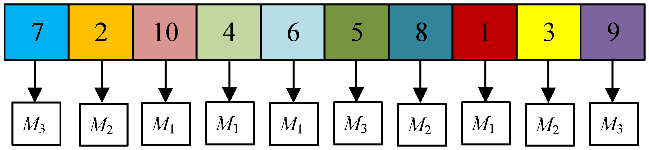
This paper uses an operation-based coding method. The gene on the chromosome represents the number of the material. The length of the chromosome is the kind of material in the material collection. The coding method has a small search space and is convenient to operate. Take the scheduling problem metal structural parts blanking workshop with feeding constraints of 10 parts and three machines as an example. As shown in Figure 2, the chromosome [7 2 10 4 6 5 8 1 3 9] represents the global priority reading sequence of the ten material types. Each chromosome corresponds to a material processing sequence. According to a certain decoding rule, it can be determined that the maximum waiting time of the machine tool is minimized under the scheduling scheme. The storage locations in the near-line buffer are not directly encoded in the chromosome; instead, they are dynamically determined during the decoding process according to the current availability of empty slots, the feeding timeline, and feasibility constraints.

Decoding is implemented via a time-driven serial generation mechanism. Materials are read sequentially according to $\pi$ and assigned to the machine that minimizes the resulting completion time and waiting penalty at the current decision point. In parallel, the crane travel time from the previous feeding location to the target machine, as well as the in-buffer reshuffling and picking times, are evaluated to determine the earliest feasible feeding time for the material. When the availability windows of the crane and the selected machine are in conflict, the feeding start time is postponed, thereby inducing the waiting time $W_{ij}$ while ensuring continuous satisfaction of both the crane single-task constraint and the machine processing constraints. If storage assignment conflicts arise due to limited near-line warehouse capacity, a repair procedure is applied, including within-batch swapping for the same machine and nearest-empty-slot filling, to restore feasibility. In rare cases where feasibility cannot be recovered, a penalized objective value is assigned, and the corresponding individual is discarded during evolution, thereby steering the search toward the feasible region.

Given a chromosome sequence $\pi$, the proposed decoding procedure transforms the encoded global order into a fully executable schedule. The decoding results provide the job–machine assignment and the processing sequence for each machine, as well as outputs the corresponding machine timing variables, including the actual start time $S_{j,i}$ and completion time $C_{j,i}$. In addition, the reshuffling and picking times implied by the selected storage positions in the line-side buffers are obtained. These outputs enable the calculation of the waiting time $W_{ij}$ and consequently, the objective value $Z$. Hence, the crane- and storage-related resource constraints are not employed merely for ex post feasibility verification; rather, they are explicitly enforced throughout decoding and are integral to schedule construction.

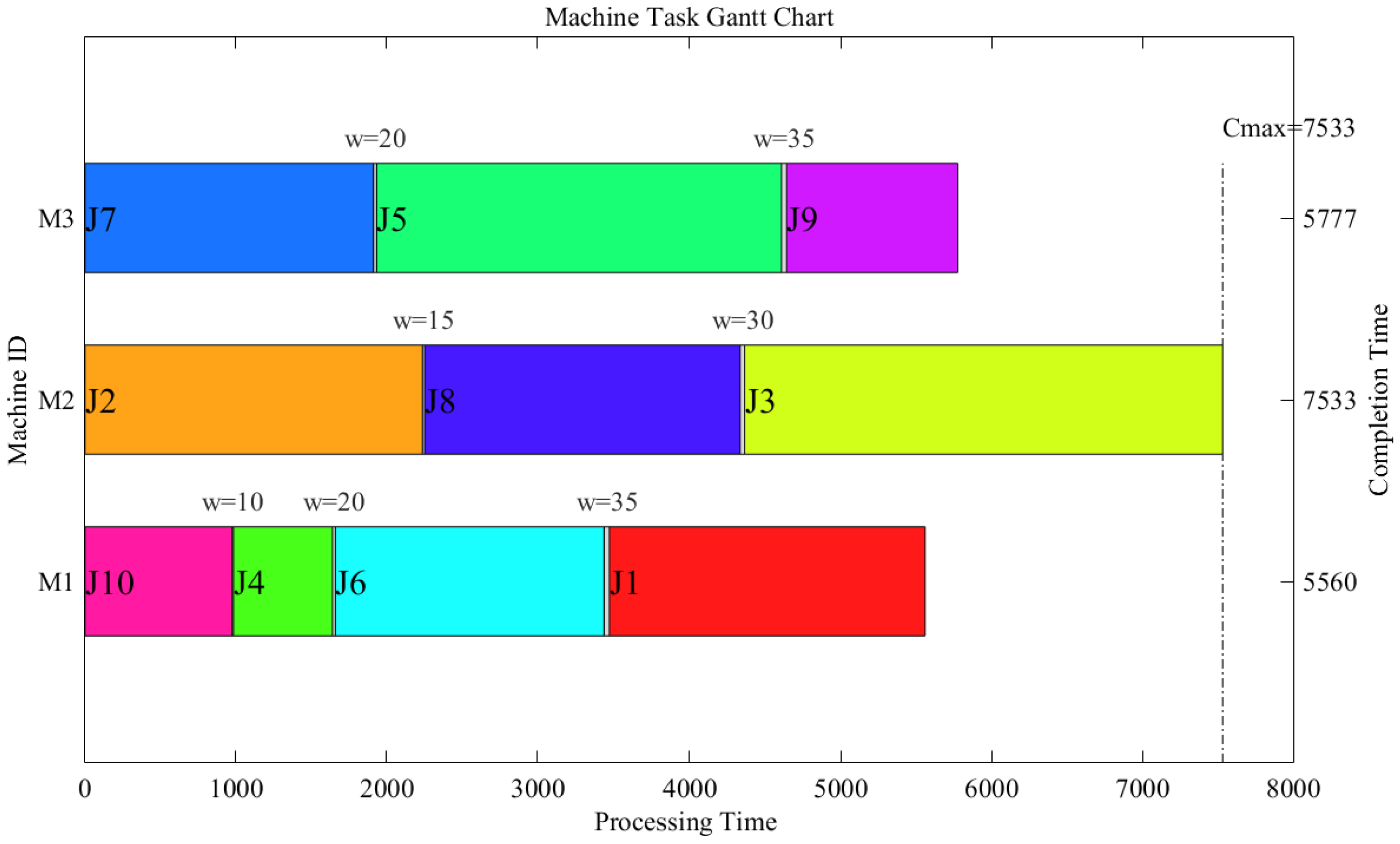
Figure 3 presents an example Gantt chart obtained by decoding a chromosome, where $J_k$ denotes the material indexed by $k$. For the same machine, the blank interval between two consecutive materials represents the machine downtime while waiting for the crane to deliver the next material, and the corresponding waiting duration is annotated in the figure. For this example schedule, the maximum waiting time among all machines is 165.

3.2. Fitness Evaluation

The optimization objective of this study is to minimize the maximum machine waiting time $Z$. To be consistent with the selection mechanism in genetic algorithms, where a larger fitness value indicates a better individual, the objective value is mapped to a fitness function $F$, defined as

$$F={\displaystyle \frac{1}{Z+1}}$$

(15)

Here, $Z$ is calculated through the decoding procedure. A small $Z$ yields a larger $F$, and thus the corresponding individual has a higher probability of being preserved and reproduced during the selection stage.

3.3. Selection

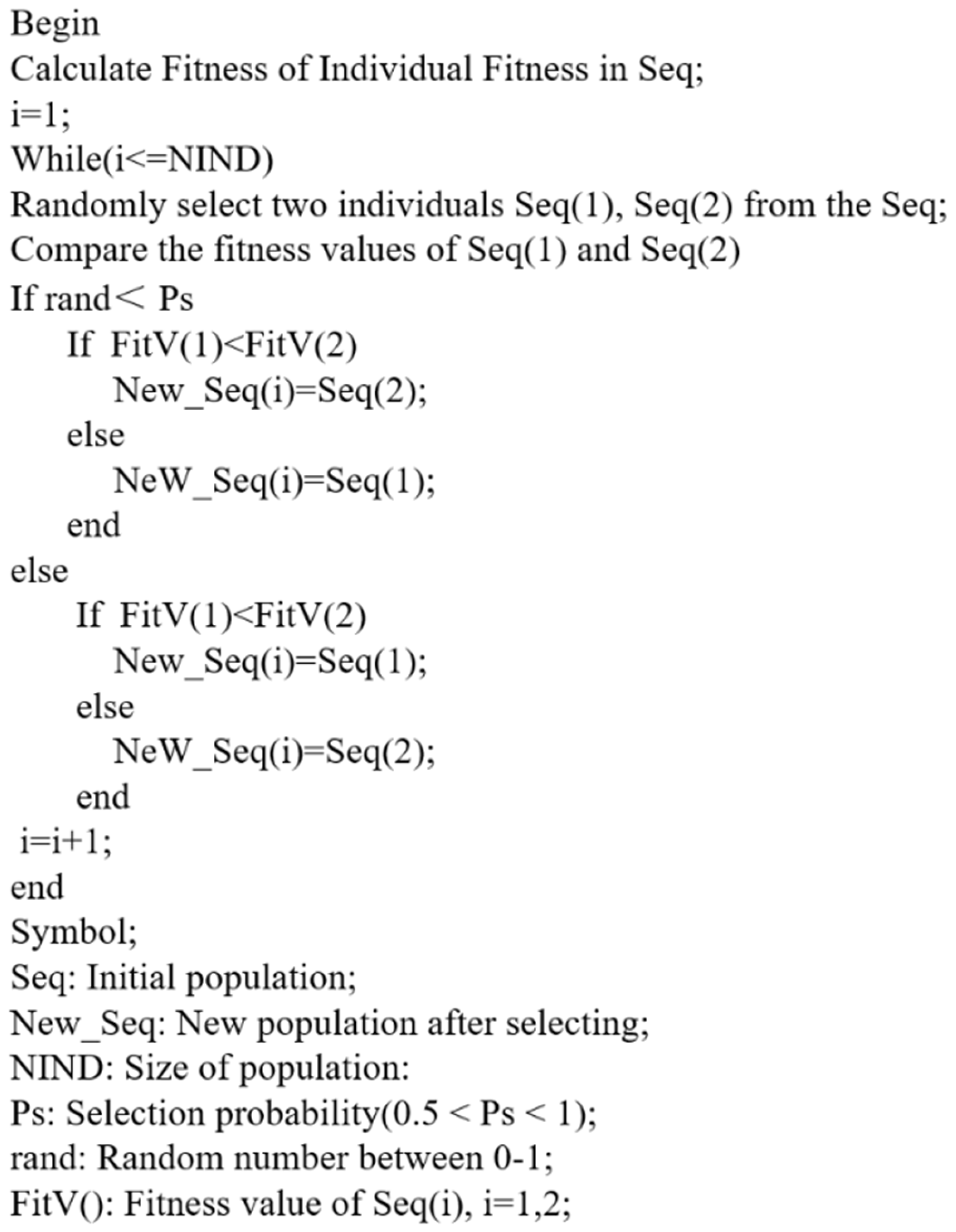
A sampling-with-replacement tournament selection scheme is adopted. In each tournament, two individuals $p_1$ and $p_2$ are randomly drawn from the population, with fitness values $F\left(p_1\right)$ and $F\left(p_2\right)$, respectively. If $F\left(p_1\right)\ge F\left(p_2\right)$, then $p_1$ is selected into the next generation with probability $p_s$, and $p_2$ is selected with probability $1-p_s$. Otherwise, if $F\left(p_1\right)<F\left(p_2\right)$, $p_2$ is selected with probability $p_s$, and $p_1$ is selected with probability $1-p_s$. Here, $p_s\in (0.5, 1)$ controls the selection pressure: a larger $p_s$ accelerates convergence but reduces population diversity more rapidly, whereas a smaller $p_s$ is more favorable for maintaining diversity. The pseudo-code diagram of the selection operation is shown in Figure 4.

3.4. Crossover and Mutation

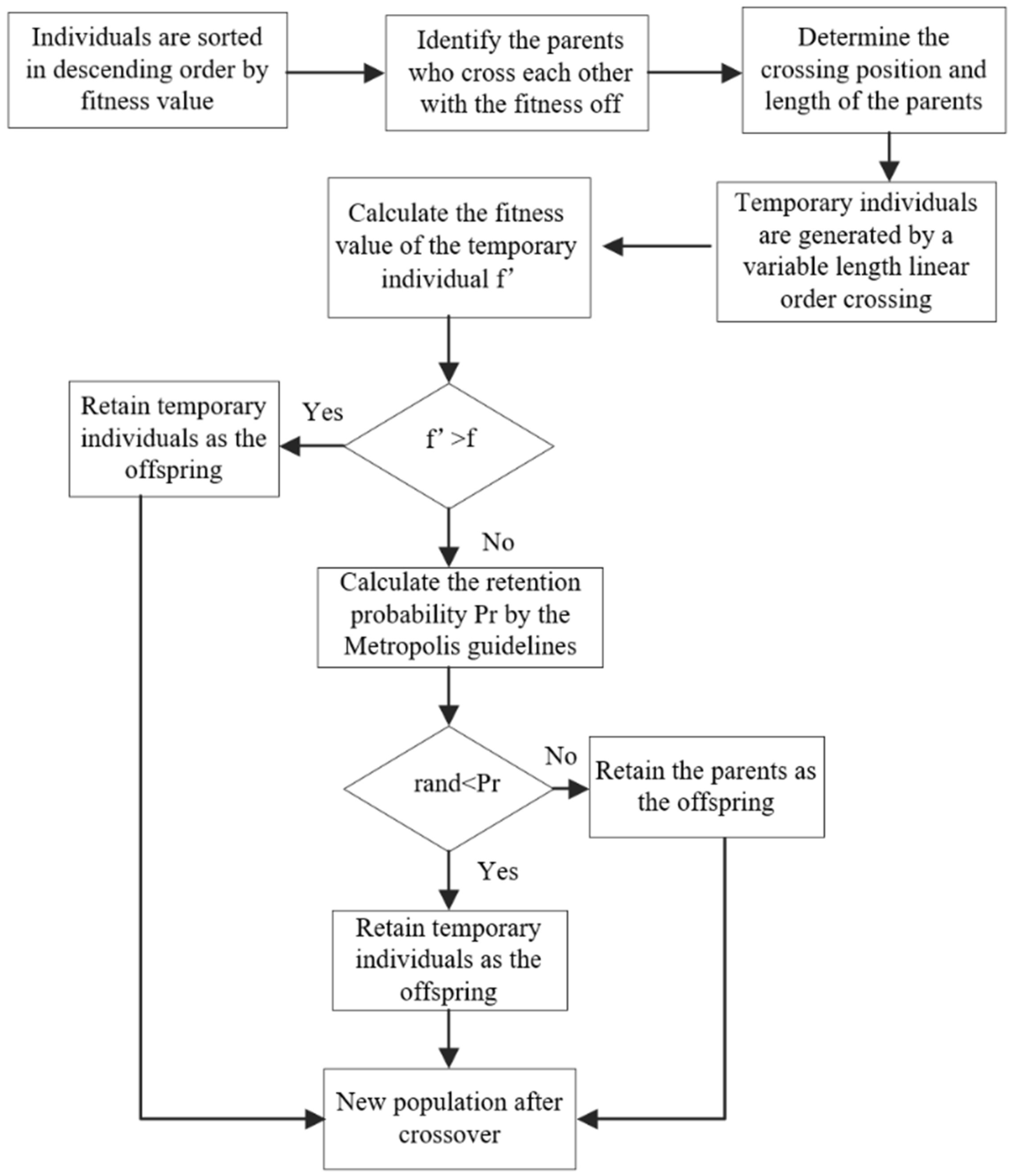
The crossover method is based on fitness-value matching: (1) The population is sorted in descending order of fitness. Parent matching is then performed according to fitness disparity, where two individuals with a relatively large fitness gap are preferentially selected as crossover parents. This strategy helps avoid repeated crossover among highly similar individuals, which may otherwise lead to premature convergence. By encouraging recombination between structurally dissimilar parents, it is more likely to generate offspring with larger structural variations, thereby maintaining population diversity and improving solution quality and stability. (2) For each selected parent pair, the crossover position and crossover length are randomly generated. A linear order crossover with variable segment length is applied to produce a provisional offspring, enabling effective recombination under different perturbation scales. (3) The objective value $Z$ and fitness $F$ of the provisional offspring are then evaluated. A simulated-annealing Metropolis acceptance criterion is incorporated to decide whether the provisional offspring is retained. The cross-operation flowchart is shown in Figure 5.

In the process of genetic algorithm evolution, the optimal individuals should be preserved as much as possible while maintaining population diversity. Therefore, this paper adopts an adaptive crossover operator and mutation operator related to generation index, and sets the minimum threshold of crossover and mutation operators. The expressions of adaptive crossover probability and mutation probability are shown in Equations (16) and (17), respectively:

$$p_c=p_c-(p_c-p_{c\min })\cdot iter/\max iter$$

(16)

$$p_m=p_m-(p_m-p_{m\min })\cdot iter/\max iter$$

(17)

$p_{c\min }$: minimum threshold for crossover probability. $p_{m\min }$: the lowest threshold of the probability of variation. $iter$: current iteration number. $\max iter$: the maximum number of iterations.

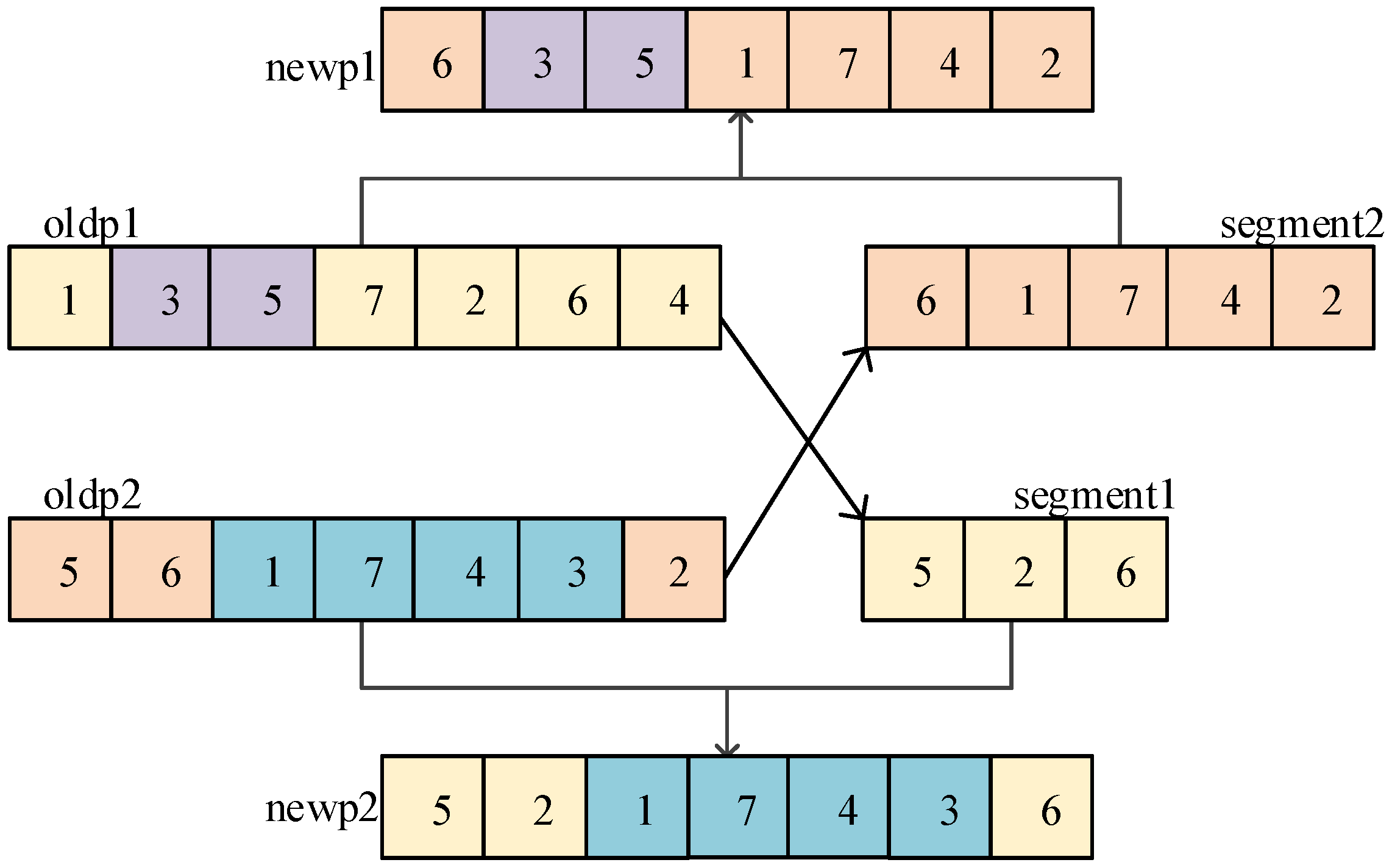
When performing the crossover operation, parents are selected according to their fitness values, and a variable-length linear order crossover is employed. Figure 6 illustrates the schematic procedure of the crossover operation. Specifically, the crossover positions and the crossover length of the two parent chromosomes, oldp1 and oldp2, are randomly selected. The chromosome segment between the two crossover positions is inherited by the offspring, newp1 and newp2, respectively. Then, the remaining genes from the other parent that do not appear in the inherited segment are copied sequentially to complete the offspring. Compared with the conventional linear order crossover, the crossover length in our operator is random and does not need to be the same for both parents. In Figure 6, the crossover positions of oldp1 are 2 and 3 with a crossover length of 2, while those of oldp2 are 3 and 6 with a crossover length of 4.

The mutation operation adopts the basic position variation, and the coding sequence of the individual is exchanged with the probability of mutation, and the positions of the two variant gene positions are randomly specified to exchange the gene values.

3.5. Simulated-Annealing-Based Acceptance Criterion

To alleviate the premature convergence of the conventional genetic algorithm caused by the loss of population diversity in later iterations, this study incorporates a simulated-annealing (SA) acceptance rule (i.e., the Metropolis criterion) after crossover and mutation generate candidate offspring. This mechanism enhances the ability to escape local optima while preserving selection pressure.

Let $Z$ denote the objective value of the current retained solution, and let $Z^{\prime }$ denote the objective value of the candidate offspring. The acceptance rule is defined as follows:

(1)

If $Z^{\prime }\le Z$, the candidate offspring is accepted unconditionally.

(2)

If $Z^{\prime }>Z$, the candidate offspring is accepted with probability $p$, where $p$ is calculated by

$$p=exp(-{\displaystyle \frac{Z\prime -Z}{T}})$$

(18)

and $T>0$ is the temperature parameter. The temperature is updated according to a geometric cooling schedule:

$$T_{k+1}=\alpha T_k, 0<\alpha <1$$

(19)

where $k$ denotes the iteration index, and $\alpha$ is the cooling factor.

This mechanism allows inferior solutions to be accepted with a relatively high probability at the early stage of the algorithm, thereby increasing search perturbations and overcoming local optimum barriers. As the iterations proceed and the temperature gradually decreases, the probability of accepting inferior solutions declines, and the algorithm’s behavior progressively shifts from global exploration to intensified local convergence. Therefore, the SA acceptance criterion can be regarded as embedding a temperature-decreasing local search into the evolutionary process, which helps improve solution quality and the stability of the algorithmic results.

4. Simulation Experiment

4.1. Parameter Settings

To verify the effectiveness of the improved genetic algorithm with fitness-value-based crossover (IGA) proposed in this paper, we randomly generate simulation instances of a metal structural part blanking workshop scheduling problem with three scales m × n: 3 × 10, 6 × 40, and 10 × 100, for simulation analysis. The processing time of each material is sampled from a uniform distribution U [500, 3000]. The generated instances are solved by IGA, the simulated-annealing genetic algorithm (SAGA), the standard genetic algorithm (GA), discrete particle swarm optimization (DPSO), and ant colony optimization (ACO). By comparing the solution results, the effectiveness and performance of IGA are evaluated.

To ensure a fair comparison, GA, SAGA, DPSO, ACO, and IGA use the same population size and maximum number of iterations for each problem scale: (10, 30) for 3 × 10, (50, 100) for 6 × 40, and (100, 200) for 10 × 100, respectively. The remaining control parameters are given in

Table 1. The parameter settings for GA, SAGA, DPSO, ACO, and IGA.

Instances of Size m × n	GA	SAGA	IGA	DSPO	ACO
3 × 10	Pc = 0.9, Pm = 0.20	Pc = 0.9, Pm = 0.20, T0 = 2000, α = 0.90	Pc0 = 0.9, Pm0 = 0.20, T0 = 2000, α = 0.90	w = 0.7, c1 = c2 = 1.5, vmax = 0.25	α = 1, β = 2, ρ = 0.2, Q = 1
6 × 40	Pc = 0.9, Pm = 0.15	Pc = 0.9, Pm = 0.15, T0 = 10,000, α = 0.90	Pc0 = 0.9, Pm0 = 0.15, T0 = 10,000, α = 0.95	w = 0.7, c1 = c2 = 1.5, vmax = 0.25	α = 1, β = 2, ρ = 0.2, Q = 1
10 × 100	Pc = 0.9, Pm = 0.20	Pc = 0.9, Pm = 0.20, T0 = 20,000, α = 0.90	Pc0 = 0.9, Pm0 = 0.20, T0 = 20,000, α = 0.97	w = 0.7, c1 = c2 = 1.5, vmax = 0.25	α = 1, β = 2, ρ = 0.2, Q = 1

, and other initial data are provided in

Table 2. The initial data.

t0	t1	t2	tv	tu	s	Ta
5	10	4	1	1	6	5

, where $s$ denotes the number of material frames in the line-side storage.

4.2. Algorithm Comparison

To evaluate the performance across the three problem scales, each instance is solved using IGA, SAGA, GA, DPSO, and ACO. To mitigate the impact of algorithmic randomness, each algorithm is executed 30 times independently for each instance. The maximum machine waiting time is employed as the primary performance indicator. Consequently, we report the best, worst, and mean values of this indicator obtained over the 30 runs, alongside its variance and the average computational time. These metrics provide a comprehensive assessment of both solution quality and algorithmic stability. The statistical results for the three problem scales are summarized in

Table 3. Comparison of experimental results on three algorithms.

Scale	Algorithm	Mean Value	Best Value	Worst Value	Variance	Running Time (s)
3 × 10	GA	133.56	126	143	20.12	0.03
	SAGA	131.53	127	139	8.88	0.08
	IGA	134.53	126	147	28.53	0.06
	DPSO	130.53	126	140	26.44	0.02
	ACO	131.36	126	138	9.74	0.03
6 × 40	GA	699.57	661	729	242.18	1.04
	SAGA	701.33	661	728	172.43	3.26
	IGA	689.66	647	722	322.29	2.82
	DPSO	702.86	674	742	230.25	0.97
	ACO	694.43	651	721	293.42	2.04
10 × 100	GA	2145.30	1887	2296	11,703.80	10.66
	SAGA	2144.50	2007	2300	5373.16	30.54
	IGA	2043.07	1782	2296	18,077.30	27.90
	DPSO	2150.00	1919	2286	9253.27	9.95
	ACO	2127.73	1797	2324	16,167.00	22.18

.

In Table 3, it is shown that for the small-scale instances, all algorithms are able to obtain solutions of comparable quality within a relatively short time, and the differences among them are marginal. As the problem scale increases, the performance discrepancies become more pronounced. Overall, IGA consistently delivers better solution quality on the medium- and large-scale instances with reduced variability, indicating improved stability and robustness. In contrast, several benchmark algorithms exhibit more noticeable performance deterioration or higher solution dispersion when applied to large-scale instances.

For the smallest instance (3 × 10), the processing times are set to part = [2084, 2237, 3169, 666, 2695, 1801, 1913, 2097, 1134, 974]. To obtain an exact benchmark solution, we perform exhaustive enumeration over all $10!$ possible job permutations. Each permutation was evaluated using the same decoding and objective-evaluation procedure as in our proposed algorithm (i.e., identical waiting-time calculation and crane feeding feasibility rules). Because the enumeration covers the entire search space, the best value is the global optimum for this instance. The exact optimum is 126, attained by the sequence [9, 1, 2, 4, 6, 10, 7, 3, 5, 8]. In total, 3,628,800 permutations were evaluated, requiring 220.37 s on our test machine. Importantly, the best solution returned by our proposed algorithm also attains an objective value of 126 on this instance (optimality gap = 0%), thereby validating the correctness of the decoding and objective-evaluation procedure and the solution quality of the proposed method. As the scheduling scale expands, the number of variables and constraints in the proposed mixed-integer linear programming model increases exponentially, leading to prohibitive computational complexity. Consequently, exact solvers demand excessive memory and computing resources, resulting in prolonged solution times that may exceed practical limits. To ensure real-world applicability, the proposed hybrid algorithm is employed to obtain high-quality near-optimal solutions within a computationally acceptable timeframe.

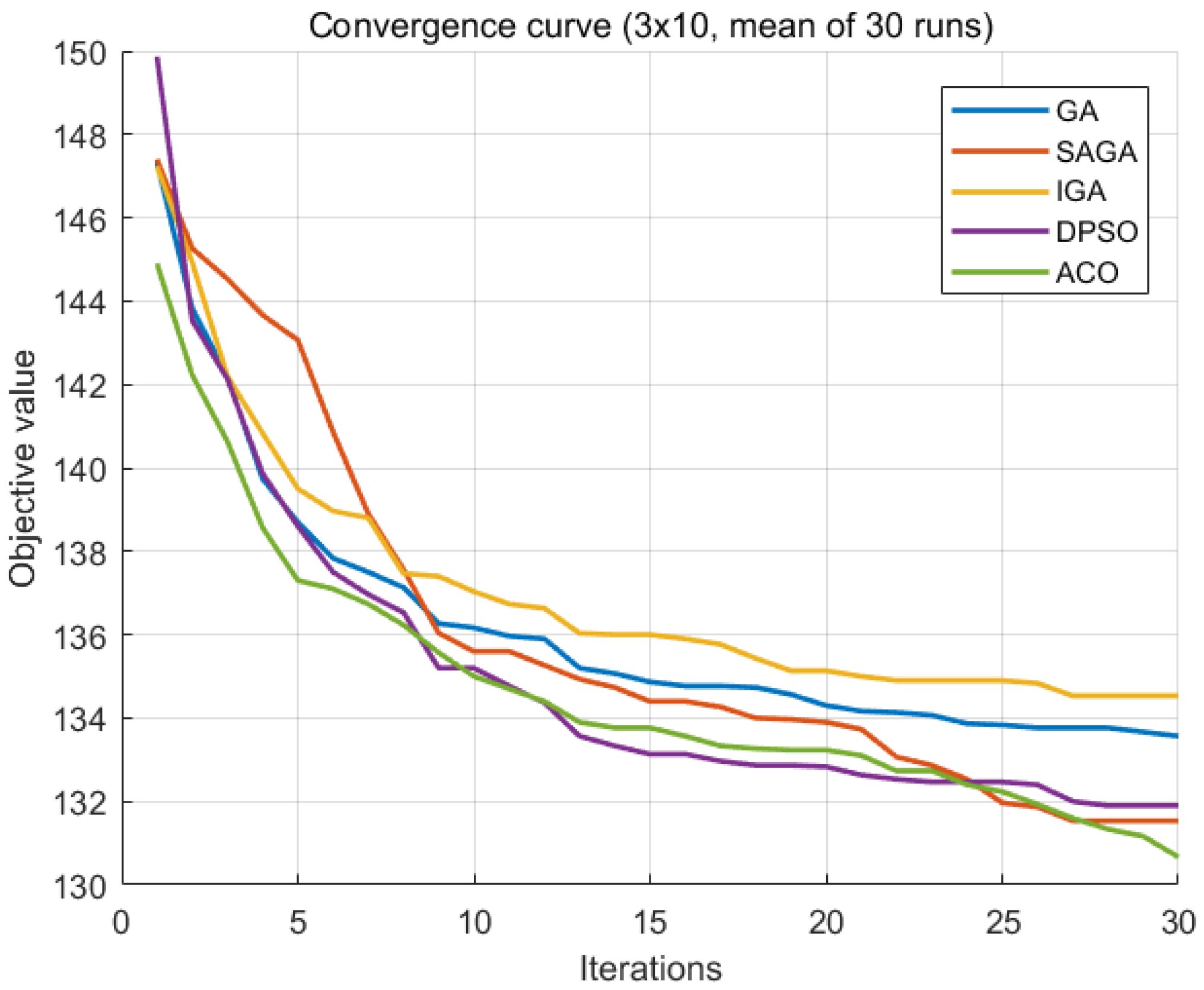
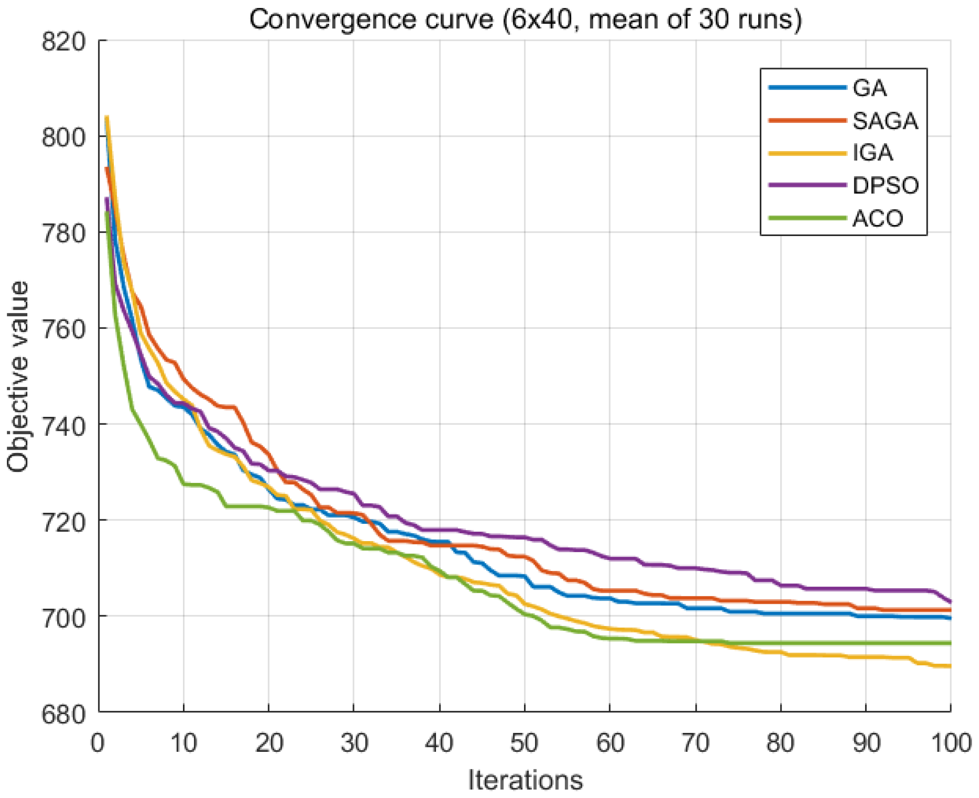
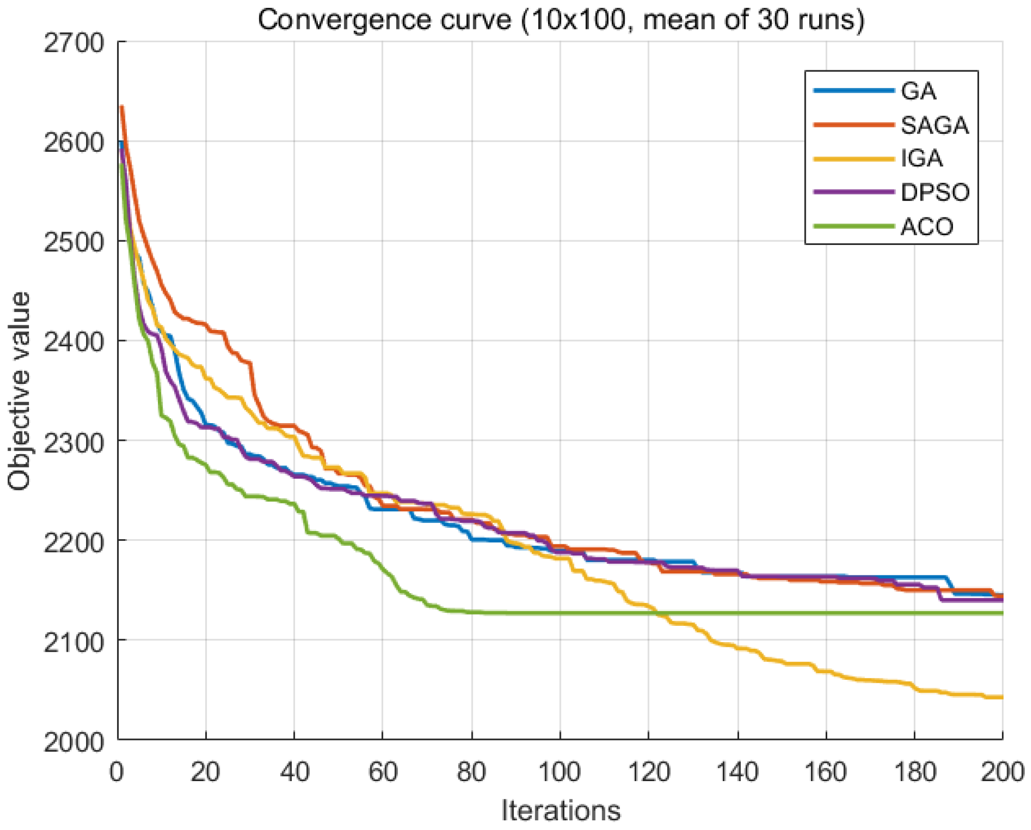
To better illustrate the performance differences, Figure 7, Figure 8 and Figure 9 report the 30-run average best-so-far convergence curves of IGA, SAGA, GA, DPSO, and ACO for three problem scales.

On the small instance (3 × 10), all methods reduce the objective quickly in the first few iterations and then converge to a similar solution level, with ACO and DPSO achieving slightly better final values, while IGA is marginally worse. As the scale increases (6 × 40 and 10 × 100), the relative advantages become more pronounced. In particular, IGA maintains a steady decrease throughout the search and continues to improve in the middle and late iterations, finally converging to the lowest objective value among all competitors. In contrast, GA shows clear stagnation in the later stage, and SAGA converges to a higher solution level. DPSO and ACO remain competitive on smaller instances, but their convergence slows noticeably as the problem size grows, leading to limited late-stage improvement and inferior final solution quality compared with IGA (especially on the 10 × 100 instance).

Overall, the results indicate that the fitness-matching crossover in IGA helps preserve population diversity while retaining high-quality individuals, and the embedded Metropolis acceptance criterion mitigates premature convergence and strengthens the ability to escape local optima. These mechanisms enable IGA to deliver consistently better performance, with its advantage becoming increasingly evident on medium- and large-scale problems.

4.3. Example Verification

In order to verify the feasibility of the scheduling model of the metal structural parts blanking workshop with the feeding constraint proposed in this paper, all algorithms were implemented in MATLAB R2017a and executed on a Windows 10 desktop computer equipped with an Intel Core i5-11400H CPU (2.7 GHz) and 16 GB RAM. The scheduling results are obtained by inputting actual production data. Due to the long processing time of the material, the machine waiting time is short compared to the material processing time, and the machine waiting time cannot be well presented in the Gantt chart. Therefore, the processing time of some materials that were processed in a metal structural parts blanking workshop on a certain day is reduced proportionally as the input to the model. There are 10 available machines in the workshop. The near-line warehouse is 3 × 3 in size and contains nine material frames. The actual production data after processing is shown in

Table 4. Production data.

Material Number	Processing Time	Material Number	Processing Time	Material Number	Processing Time	Material Number	Processing Time
J1	2000	J2	1820	J3	3045	J4	1260
J5	780	J6	1560	J7	2955	J8	2655
J9	3245	J10	1440	J11	945	J12	2405
J13	3125	J14	960	J15	1705	J16	2900
J17	3015	J18	1620	J19	1665	J20	2185

.

According to the above model and solving algorithm, the maximum waiting time of the machine tool under the optimal scheduling scheme is 170. The waiting time of each batch of materials processed by the machine tool is shown in

Table 5. Waiting time.

		1	2	3	4	5	6	7
$M_1$		0	25	20	25	15	20	-
$M_2$		0	15	20	40	50	15	-
$M_3$		0	40	30	40	25	35	-
$M_4$		0	20	30	25	25	30	20
$M_5$		0	30	20	15	30	25	-
$M_6$		0	25	35	30	15	-	-
$M_7$		0	35	20	15	20	20	40
$M_8$		0	20	20	20	15	35	25
$M_9$		0	15	45	30	40	-	-
$M_{10}$		0	40	15	50	40	-	-

. In Table 5, the column represents the machine tool, the row represents the processing batch of the machine tool, and “-” means that the processing batch does not exist in the machine tool.

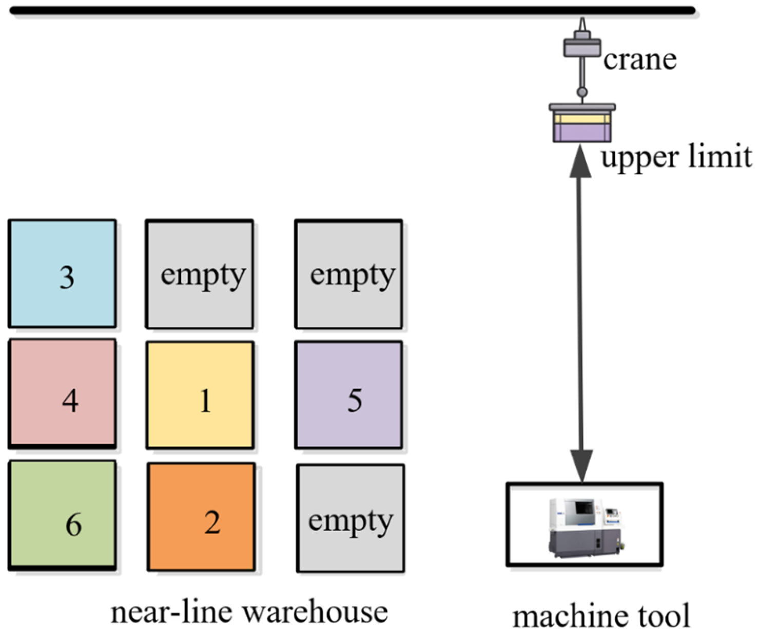
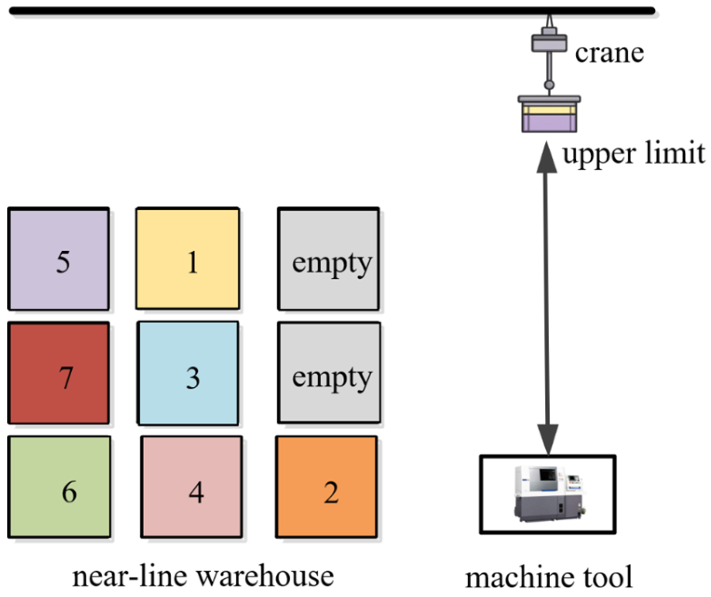
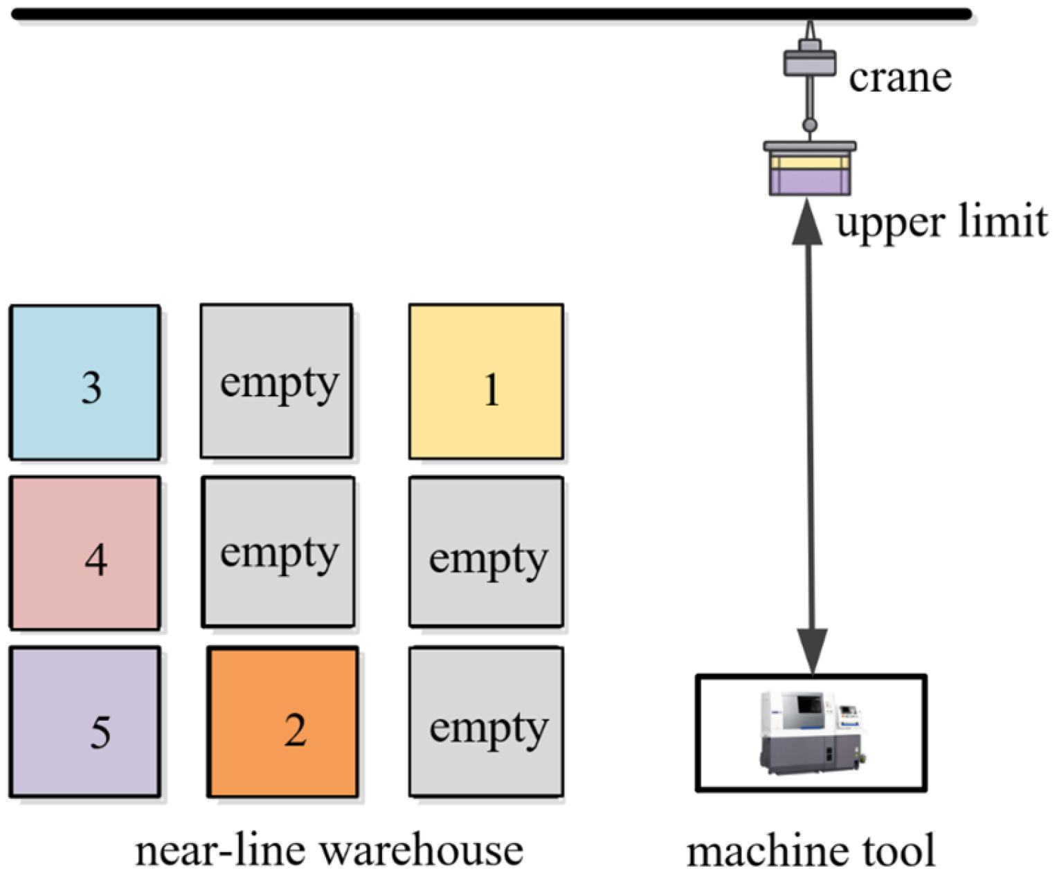
The position of materials in the near-line warehouse is determined by the batch of material in the near-line warehouse. Six batches of materials are processed on machine tools M₁, M₂, M_3, and M₅; the position of materials in the near-line warehouse is shown in Figure 10. Seven batches of materials are processed on machine tools M₄, M_7, and M₈; the position of materials in the near-line warehouse is shown in Figure 11. Five batches of materials are processed on machine tools M₆, M_9, and M₁₀; the position of materials in the near-line warehouse is shown in Figure 12. In Figure 10, Figure 11 and Figure 12, the number “1” indicates that the first batch of material processed by the machine tool is placed in this position, and “empty” indicates that the material frame at this position does not store the material. For example, the material processed by machine tool M₁ is J12, J8, J27, J14, J5, and J22 in turn, and the storage location of the material is shown in Figure 13.

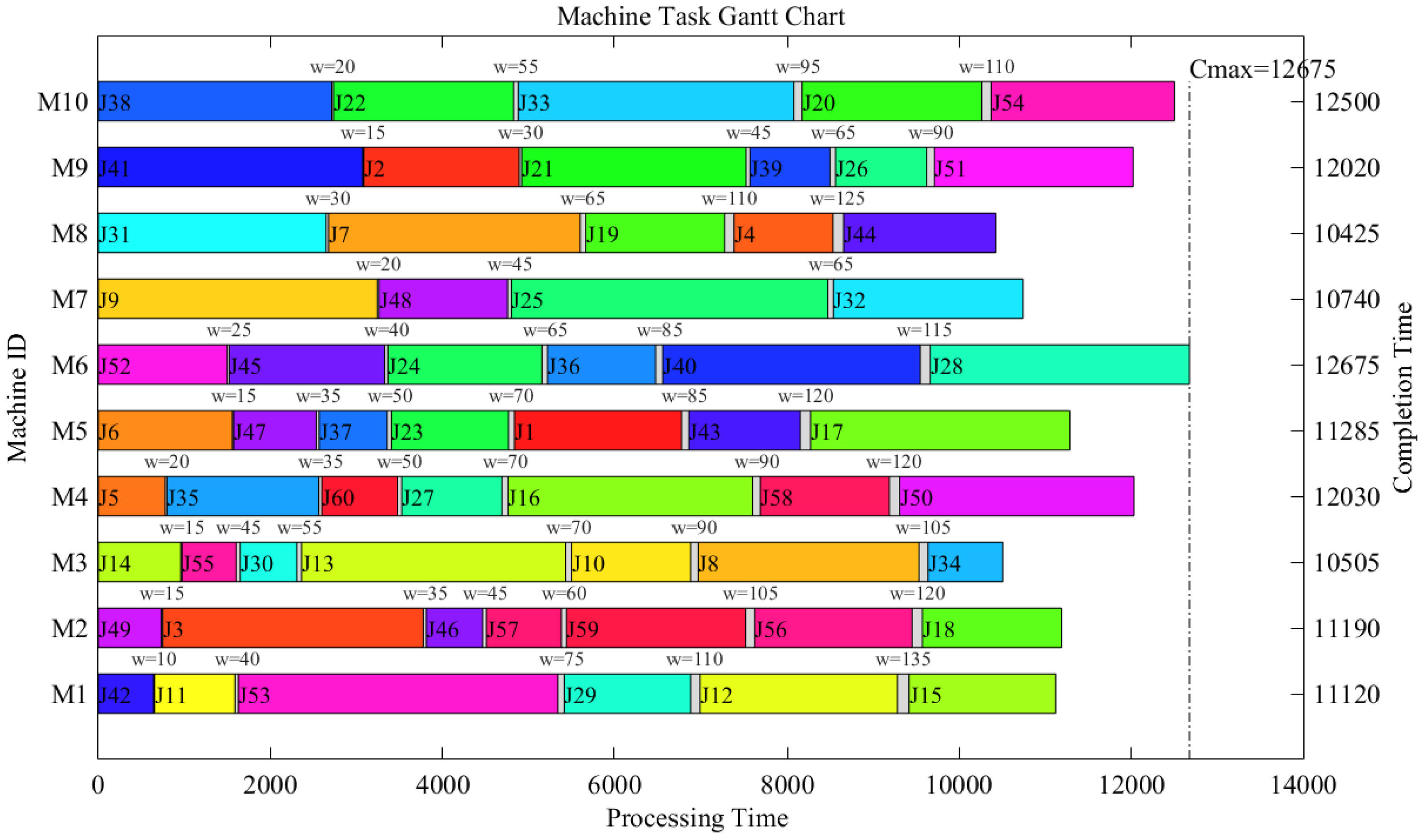
The Gantt chart of the near-optimal scheduling scheme obtained by the proposed algorithm is shown in Figure 14. Among them, J1~J60 is the material number, J33 and J36 respectively represent the first batch of material number and the second batch of material number processed by machine tool M_10. The blank space between material J33 and J36 represents the waiting time when the machine tool is preparing material J36, which is 40.

5. Conclusions

This research investigates the integrated scheduling problem within a metal structural parts blanking workshop. The primary findings and conclusions of this study are summarized as follows:

(1)

This study focuses on a metal structural parts’ blanking workshop. To address the limited feeding capacity of a single overhead crane and the feeding-time variability caused by heterogeneous line-side buffer locations, we formulate an integrated scheduling model that explicitly incorporates in-buffer reshuffling and picking times as well as crane travel constraints, with the objective of minimizing the maximum machine waiting time. The model jointly determines the material processing sequence and the storage positions in line-side buffers, thereby mitigating machine downtime due to material shortages from a mechanistic perspective.

(2)

Given the discrete combinatorial nature of the model, an improved genetic algorithm is developed with fitness-matching crossover, and a simulated-annealing acceptance rule is embedded to enhance global search capability. For over 30 independent runs on randomly generated instances of varying scales, the proposed algorithm achieves smaller maximum waiting times and better stability, particularly for medium- and large-scale cases.

(3)

Simulation results further indicate that, when combined with a storage-position optimization strategy guided by batch-to-buffer mapping, the proposed approach can effectively shorten crane feeding time and improve machine utilization. Overall, this work provides a practical modeling and solution framework for feeding-constrained scheduling in machining workshops with line-side buffers.

Future work will proceed in three directions:

(1)

incorporating more refined material-handling mechanisms into the model, including crane acceleration and deceleration, obstacle avoidance, and multi-crane coordination;

(2)

investigating real-time scheduling under uncertain processing times and dynamic job insertions;

(3)

further developing hybrid frameworks that integrate more advanced metaheuristics with exact algorithms, and conducting comparative validation on additional real-world production datasets.