Pore-Scale Investigation and Application of Two-Phase Low-Velocity Non-Darcy Flow in Low-Permeability Porous Media

Abstract

The widely applied empirical Darcy’s law in geotechnical engineering faces significant challenges in describing low-velocity flow processes in low-permeability porous media such as tight sandstones containing irreducible water. A deep understanding of low-velocity non-Darcy two-phase flow behavior in low-permeability porous media is essential for evaluating the development of ultra-low-permeability reservoirs. In this study, seven low-permeability three-dimensional digital cores with distinct pore structures were constructed based on realistic ultra-low-permeability sandstones. Using the lattice Boltzmann method, pore-scale investigations of water displacing oil were conducted. Low-velocity two-phase flow behavior under varying wettability conditions, pore structures, and fluid viscosities was simulated. The underlying mechanisms of low-velocity non-Darcy flow in ultra-low-permeability sandstones were examined, leading to a modified low-velocity non-Darcy flow equation. This improved model was subsequently applied to numerical simulations of ultra-low-permeability reservoirs. The results demonstrate that non-Darcy effects manifest primarily as nonlinearities in seepage curves, representing a marked departure from conventional Darcy’s law. Low-velocity non-Darcy (LVND) flow is predominantly constrained by the influence of complex pore-throat structures and capillary forces on fluid distribution. The dynamic equilibrium among capillary forces arising from residual water saturation, viscous forces, and pressure gradients constitutes the fundamental mechanism governing the onset of LVND flow. Enhanced nonlinear behavior is observed with increasing viscosity of the invading phase and elevated capillary forces. Substantial discrepancies in reservoir production dynamics are identified between LVND and classical Darcian regimes. Through pore-scale numerical simulations, this study systematically elucidates LVND behavior during bi-phasic flow in low-permeability porous media, while identifying critical controlling factors. These findings provide scientific rationale and technical support for addressing geological engineering challenges in tight sandstone formations.

1. Introduction

Darcy’s law, an empirical principle describing fluid flow through porous media, is extensively applied in hydrology, geotechnical engineering, and energy extraction [1]. It establishes a linear relationship between fluid flow velocity, the permeability of the medium, and the pressure gradient. Flow characterized by this linear relationship is referred to as Darcy flow. However, low-permeability porous media such as tight sandstones typically exhibit low porosity and low permeability, along with more complex pore structures. These attributes cause fluid flow at low velocities to deviate significantly from that in conventional porous media, resulting in a nonlinear relationship between velocity and pressure gradient—a phenomenon known as LVND flow [2]. In such media, fluid flow is governed by multiple factors, including pore geometry, wettability, and fluid properties [3,4]. Under low-flow-rate conditions, capillary effects and interfacial tension emerge as dominant mechanisms controlling flow behavior, rendering Darcy’s law inadequate for accurately describing bi-phasic flow in these systems [5].

Numerous studies have been conducted to characterize low-velocity non-Darcy flow, which can be broadly classified into two categories: macroscopic model studies and pore-scale studies. The nonlinear flow regime observed under sub-Darcy conditions is characterized by two principal phenomena: the threshold pressure gradient (TPG) and a nonlinear velocity–pressure relationship at low flow rates, which collectively give rise to two distinct flow states—namely, the no-flow condition and pre-Darcy flow. A variety of models have been proposed in the literature to characterize sub-Darcy flow behavior, among which the TPG model and the pre-Darcy flow model are most widely recognized. The concept of TPG originates from the earlier notion of threshold pressure, initially documented in the 1950s [6]. It was formally introduced as TPG by [7], who modified the classical Darcy equation by shifting the linear flow relation relative to the origin. Owing to its mathematical simplicity, the TPG model has been extensively adopted as a foundational approach for describing LVND flow [8,9]. Subsequent studies have further developed its applicability. Shi et al. [10] established an empirical correlation between the pseudo-threshold pressure gradient and permeability through experimental investigations and analyzed its influence on production performance. More recently, Xiao et al. [11] developed a numerical simulation model for fractured horizontal wells that incorporates TPG and stress-sensitive effects, demonstrating improved accuracy in predicting well productivity. Geng et al. [12] incorporated the TPG effect into their analysis of pressure transient responses in tight sandstone oil wells, demonstrating improved alignment with field data. Due to its linear formulation for sub-Darcy flow, the TPG model has been widely adopted in reservoir numerical simulation and pressure transient analysis [13,14]. Subsequently, Jiang et al. [15] introduced a two-parameter non-Darcy flow model that accounts for boundary-layer effects and non-Bingham fluid behavior. Li et al. [16] applied Jiang’s model to pressure transient analysis in dual-porosity reservoirs and proposed a numerical simulation approach using traditional Cartesian grids. Further refinements were made by Liu et al. [17], who reformulated Jiang’s equation into a new form in which the non-Darcy term is characterized by three parameters, and implemented it in a dual-medium model for pressure transient analysis. Dejam et al. [18] developed an analytical model for steady-state flow of slightly compressible fluids under linear and radial pre-Darcy flow conditions, deriving closed-form solutions through a generalized Boltzmann transformation technique. Ma et al. [19] integrated sub-Darcy flow behavior into an EDFM approach, applying it to flow diagnostics for well placement optimization and enhanced oil recovery strategies. Existing findings indicate that irreducible water saturation and electro-viscous effects constitute the primary mechanisms governing pre-Darcy flow behavior [20]. Most recently, Fan et al. [21] proposed a modified and more mathematically concise pre-Darcy flow equation to characterize nonlinear flow phenomena in low-permeability reservoirs.

In pore-scale studies, researchers have focused on revealing the microscopic mechanisms of low-velocity non-Darcy flow. Through experimental investigation, Boettcher et al. [5] identified that the critical Reynolds number for the onset of sub-Darcy flow behavior is below 1 × 10⁻⁹, establishing a definitive threshold for the transition to non-Darcy flow at ultra-low velocities. Wang et al. [22] proposed a nonlinear pre-Darcy flow model initiating from zero pressure gradient by considering boundary-layer effects and applied it to well productivity prediction. Despite its extensive application, the TPG model is limited to characterizing the no-flow regime and the linear Darcian flow segment and fails to represent the nonlinear pre-Darcy flow behavior. To address this limitation, Shi et al. [14] developed a sub-Darcy flow equation for low-permeability oilfields by integrating a nonlinear flow model with a pore-throat density distribution function, incorporating both boundary-layer effects and heterogeneous capillary phenomena. In a critical review of existing literature, Zhao et al. [2] incorporated both boundary-layer parameters and the TPG into the pre-Darcy flow regime and conducted coupled modeling of sub-Darcy flow in matrix systems and Darcian flow in fractures using an automatic differentiation framework. Yang et al. [20] established quantitative relationships between pre-Darcy flow parameters and aqueous-phase permeability, analyzing the coupled effects of mineral composition and pore structure in both sandstone and shale formations.

While the aforementioned studies have significantly advanced our understanding of sub-Darcy flow phenomena, existing research has predominantly focused on its engineering applications in geological contexts. Due to inherent system complexity and experimental limitations, the fundamental mechanisms and controlling factors governing sub-Darcy flow remain inadequately understood [23]. Moreover, current models—largely derived from macroscopic physical experiments or theoretical deductions—lack mechanistic validation. A comprehensive understanding of these complex nonlinear flow processes requires fundamental investigation into bi-phasic low-velocity flow through porous media to elucidate the underlying nonlinear flow physics and influencing parameters [24]. To date, few studies have systematically examined the origin and controlling factors of sub-Darcy flow at the pore scale [25]. Pore-scale numerical simulation emerges as a powerful microscopic approach that reconstructs actual fluid pathways through porous structures, captures interfacial dynamics within complex pore networks, and resolves nonlinear characteristics in flow curves. This methodology offers unprecedented potential for unraveling the mechanistic basis of sub-Darcy flow behavior [26].

This study employs the lattice Boltzmann method to simulate sub-Darcy flow behavior of bi-phasic fluids within three-dimensional, low-permeability porous media at the pore scale, with particular focus on the nonlinear relationship between pressure gradient and flow velocity under low-flow-rate conditions. The primary objectives are to elucidate the underlying mechanisms of sub-Darcy flow, comprehensively analyze the influence of pore geometry, fluid viscosity, and capillary forces, and quantitatively characterize its micro-mechanisms and macroscopic manifestations. The findings are expected to provide fundamental technical support for addressing engineering and geological challenges in low-permeability formations.

2. Methodology

Given the geometric complexity inherent in realistic three-dimensional porous media, conventional macroscopic computational fluid dynamics (CFD) approaches face significant challenges in mesh generation and computational efficiency when simulating fluid flow through such structures. The lattice Boltzmann method (LBM), with its meshless nature and inherent compatibility with graphics processing unit (GPU) parallelization, offers a particularly suitable framework for pore-scale flow simulations [27].

The color-gradient model demonstrates distinct advantages in simulating immiscible two-phase flow systems characterized by large density and viscosity contrasts. This study adopts the Gunstensen color-gradient model to simulate displacement processes in low-permeability porous media [28]. Within this framework, different fluid phases are distinguished by distinct color labels. Interfacial interactions are modeled by introducing a color gradient, which directs the evolution of particle distribution functions to achieve phase separation or mixing.

Notably, the color-gradient multi-phase model enables independent adjustment of surface tension and viscosity, maintains sharp interfacial profiles between immiscible fluids, and supports efficient parallelization across computing architectures—attributes that make it especially suitable for simulating high-viscosity-ratio immiscible flow in porous media [29,30]. Furthermore, the multiple-relaxation-time (MRT) collision scheme significantly enhances numerical stability and suppresses spurious velocities at phase interfaces. Among the various multi-phase LBM formulations, the color-gradient model offers a distinct balance of accuracy and physical fidelity for immiscible two-phase flow simulations in complex porous media. In contrast, the Shan–Chen pseudopotential model, while computationally efficient, suffers from inherent limitations such as thermodynamic inconsistency and spurious currents near the phase interface [29,31]. The free-energy model ensures thermodynamic consistency but is numerically less efficient and requires careful parameter calibration. Given the need to accurately capture low-velocity non-Darcy flow behavior—where capillary effects and interfacial dynamics are dominant—the color-gradient model is therefore the most appropriate choice for this study, as it provides reliable interface tracking and flexible control of interfacial tension and wettability [32,33].

Interfacial tension in oil–water systems is represented using the continuum surface force (CSF) model [34]. This section elaborates on the development of an MRT-based color-gradient model incorporating the CSF formulation for simulating oil–water two-phase flow in tight sandstone porous media.

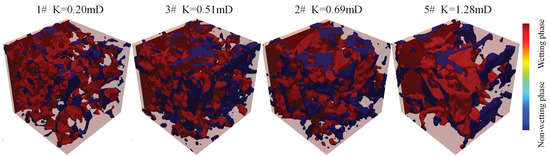
2.1. Two-Phase Color-Gradient Lattice Boltzmann Model

In the color-fluid model, distinct fluid phases are identified by color labels—for instance, red (r) and blue (b) fluids—each represented by its own set of PDFs, denoted as f_i^r and f_i^b, where the subscript i indicates the i-th lattice direction. The total PDF of the fluid mixture at position (x, t) is given by

$$f_i\left(x,t\right)=f_i^r\left(x,t\right)+f_i^b\left(x,t\right),$$

(1)

The lattice Boltzmann equations governing the evolution of the red and blue fluids are formulated as follows:

$$f_i^s\left(x+{\mathit{e}}_i\delta t,t+\delta t\right)=f_i^s\left(x,t\right)+{\mathrm{\Omega }}_i^s\left(x,t\right),s=r,b,i=0,\dots ,18,$$

(2)

where s represents fluid r or fluid b; δ_t is the time step; e_i is the lattice vector of the D3Q19 model. The distribution function of fluid $f_i\left(x,t\right)$ in the i-th velocity direction at position x and time t is the collision operator ${\mathrm{\Omega }}_i^s\left(x,t\right)$.

The collision operator in the color-fluid model comprises three constituent terms:

$${\mathrm{\Omega }}_i^s={\mathrm{\Omega }}_i^{s(3)}\left\{{\mathrm{\Omega }}_i^{s(1)}+{\mathrm{\Omega }}_i^{s(2)}\right\},$$

(3)

where ${\mathrm{\Omega }}_i^{s(1)}$ is an SRT collision operator; ${\mathrm{\Omega }}_i^{s(2)}$ is a perturbation operator responsible for generating interfacial tension; ${\mathrm{\Omega }}_i^{s(3)}$ is a recoloring operator that enforces phase segregation by redistributing particle populations.

The conservation of mass and total momentum for each fluid must meet the following conditions:

$$\left\{\begin{array}{l}{\rho }_r={\displaystyle \sum _i{f}_i^r},{\rho }_b{\displaystyle \sum _i{f}_i^b}\\ \rho \mathit{u}={\displaystyle \sum _s{\displaystyle \sum _i{f}_i^{s,eq}{\mathit{e}}_i}}\end{array}\right.,$$

(4)

where ρ_r represents the density of the fluid in phase r. ρ_b represents the density of the fluid in phase b. ρ is the total fluid density; u is the local fluid velocity.

By satisfying the conservation constraints of mass conservation and total momentum conservation, the following equilibrium distribution function is selected:

$$f_i^{s,eq}={\rho }_s{w}_i\left[1+{\displaystyle \frac{3}{c^2}}{\mathit{e}}_i\cdot \mathit{u}+{\displaystyle \frac{9}{2c^4}}{\left({\mathit{e}}_i\cdot \mathit{u}\right)}^2-{\displaystyle \frac{3}{2c^2}}{\mathit{u}}^2\right],$$

(5)

where $w_i$ is the weight factor; c is the lattice velocity, $c=\delta x/\delta t$; $\delta x$ the is lattice length.

With the total distribution function, the single-phase collision and perturbation operators are generally approximated by BGK and can be expressed as

$${\mathrm{\Omega }}_i^{(1)}=-{\displaystyle \frac{1}{\tau }}\left(f_i-f_i^{eq}\right),$$

(6)

The MRT scheme has gained widespread adoption in simulating multi-phase and multicomponent flows due to its superior performance in enhancing numerical stability and suppressing spurious velocities at phase interfaces compared to the BGK approximation. Within the MRT framework, the collision operator ${\mathrm{\Omega }}_i^{(1)}$ is formulated as follows:

$${\mathrm{\Omega }}_i^{(1)}=-{\mathit{M}}^{-1}\mathit{S}\left(\mathit{M}f-{\mathit{m}}^{eq}\right),i=0,\dots ,18,$$

(7)

where M contains the transformation matrix of density, momentum, energy and flux; S is the collision diagonal matrix; the m^eq balance moment is calculated by ${\mathit{m}}^{eq}=\mathit{M}{f}^{eq}$.

The moment m of the distribution function is expressed as

$$m=\left(\rho ,e,ϵ,j_x,q_x,j_y,q_y,j_z,q_z,3p_{xx},3{\pi }_{xx},p_{ww},{\pi }_{ww},p_{xy},p_{yz},m_x,m_y,m_z\right),$$

(8)

These parameters correspond to density, energy, energy square, momentum, heat flux and momentum flux. Among them, $j={\rho }_0\left(u_x,u_y,u_z\right)$ is momentum, ${\rho }_0$ is the reference density constant, and $p=c^2\rho /3$ is pressure.

The balancing torque is given by the following formula:

$$\left\{\begin{array}{l}{m}_0^{eq}=\rho ,m_1^{eq}=e^{eq}=-11\rho +19{\rho }_0\left(u_x^2+u_y^2+u_z^2\right)\\ m_2^{eq}={ϵ}^{eq}=3\rho -{\displaystyle \frac{11}{2{\rho }_0\left(u_x^2+u_y^2+u_z^2\right)}},\\ m_3^{eq}={\rho }_0{u}_x,m_4^{eq}=-{\displaystyle \frac{2}{3}}{\rho }_0{u}_x,m_5^{eq}={\rho }_0{u}_y,m_6^{eq}=-{\displaystyle \frac{2}{3}}{\rho }_0{u}_y\\ m_7^{eq}={\rho }_0{u}_z,m_8^{eq}=-{\displaystyle \frac{2}{3}}{\rho }_0{u}_z,m_9^{eq}=3p_{xx}^{eq}={\rho }_0\left(2u_x^2-u_y^2-u_z^2\right)\\ m_{10}^{eq}=-{\displaystyle \frac{3}{2}}{p}_{xx}^{eq}=-{\displaystyle \frac{3}{2}}{\rho }_0\left(2u_x^2-u_y^2-u_z^2\right),m_{11}^{eq}=p_{zz}^{eq}={\rho }_0\left(u_y^2-u_z^2\right)\\ m_{12}^{eq}=-{\displaystyle \frac{1}{2}}{p}_{zz}^{eq}=-{\displaystyle \frac{1}{2}}{\rho }_0\left(u_y^2-u_z^2\right)\\ m_{13}^{eq}=p_{xy}^{eq}={\rho }_0{u}_x{u}_y,m_{14}^{eq}=p_{yz}^{eq}={\rho }_0{u}_y{u}_z\\ m_{15}^{eq}=p_{xz}^{eq}={\rho }_0{u}_x{u}_y,m_{16}^{eq}=m_{17}^{eq}=m_{18}^{eq}=0\end{array}\right.,$$

(9)

The collision diagonal matrix S is a diagonal collision matrix composed of relaxation frequencies. Other relaxation frequencies in the equation can be adjusted to improve accuracy and stability. The relaxation frequency is defined as the reciprocal of the relaxation time $S_{\nu }=1/\tau$. S is represented as

$$S=diag\left(0,S_e,S_{\xi },0,S_q,0,S_q,0,S_q,S_v,S_{\pi },S_v,S_{\pi },S_v,S_v,S_v,S_m,S_m,S_m\right),$$

(10)

For flow in porous media, the following relaxation frequencies are widely used because they can generate absolute permeability independent of viscosity:

$$S_e=S_{\xi }=S_{\pi }=S_{\nu },$$

(11)

$$S_q=S_m=8{\displaystyle \frac{\left(2-S_{\nu }\right)}{\left(8-S_{\nu }\right)}},$$

(12)

Based on the continuum surface force (CSF) concept and constrained by mass and momentum conservation principles, ref. [35] derived a generalized perturbation operator for the D3Q19 lattice ${\mathrm{\Omega }}_i^{s\left(2\right)}$, defined as

$${\mathrm{\Omega }}_i^{s\left(2\right)}={\displaystyle \frac{A_k}{2}}\left|\mathit{C}\right|\left[w_i{\displaystyle \frac{{\left({\mathit{e}}_i\cdot \mathit{C}\right)}^2}{{\left|\mathit{C}\right|}^2}}-{\displaystyle \frac{5}{9}}\right],$$

(13)

Here, C represents the color gradient, which is calculated in the following way:

$$\mathit{C}={\displaystyle \frac{3}{c^2\delta t}}{\displaystyle \sum _i{w}_i{\mathit{e}}_i\varphi \left(t,\left(x+{\mathit{e}}_i\delta t\right)\right)},$$

(14)

ϕ is the phase field order parameter of the color gradient, defined as

$$\varphi ={\displaystyle \frac{{\rho }_r-{\rho }_b}{{\rho }_r+{\rho }_b}},$$

(15)

To calculate the surface tension term, a phase field gradient is required. The surface tension is generated through perturbation based on the phase field gradient. The additional term of surface tension is [36]

$$\left\{\begin{array}{l}{m}_1^{st}=-19\sigma \left|\mathit{C}\right|\left(n_x^2+n_y^2+n_z^2\right)\\ m_9^{st}={\displaystyle \frac{1}{2}}\sigma \left|\mathit{C}\right|\left(2n_x^2-n_y^2-n_z^2\right)\\ m_{11}^{st}={\displaystyle \frac{1}{2}}\sigma \left|\mathit{C}\right|\left(n_y^2-n_z^2\right)\\ m_{13}^{st}={\displaystyle \frac{1}{2}}\sigma \left|\mathit{C}\right|n_x{n}_y\\ m_{14}^{st}={\displaystyle \frac{1}{2}}\sigma \left|\mathit{C}\right|n_y{n}_z\\ m_{15}^{st}={\displaystyle \frac{1}{2}}\sigma \left|\mathit{C}\right|n_x{n}_z\end{array}\right.,$$

(16)

Here, σ is the surface tension. n is the normalized phase field gradient, denoted as

$$n={\displaystyle \frac{\mathit{C}}{\left|\mathit{C}\right|}},$$

(17)

The expression of interfacial tension σ is as follows:

$$\sigma ={\displaystyle \frac{2}{9}}A\tau c^4\delta t,$$

(18)

Here, $A={\displaystyle {\sum }_k{A}_k}$.

The above formulation demonstrates that the interfacial tension can be flexibly regulated through parameter A.

While the perturbation operator generates interfacial tension, it does not inherently guarantee immiscibility between the two fluid phases. To promote phase segregation and maintain sharp interfacial boundaries, a recoloring operator ${\mathrm{\Omega }}_i^{\left(3\right)}$ is applied. This operator ensures distinct phase interfaces while preventing mutual dissolution of the fluids. The recoloring operators for the red and blue fluids are defined as follows [30]:

$${\mathrm{\Omega }}_i^{r\left(3\right)}\left(f_i^r\right)={\displaystyle \frac{{\rho }_r}{\rho }}{f}_i^{*}+\beta {\displaystyle \frac{{\rho }_r{\rho }_b}{{\rho }^2}}\cos \left({\phi }_i\right)f_i^{eq},$$

(19)

$${\mathrm{\Omega }}_i^{b\left(3\right)}\left(f_i^b\right)={\displaystyle \frac{{\rho }_b}{\rho }}{f}_i^{*}+\beta {\displaystyle \frac{{\rho }_r{\rho }_b}{{\rho }^2}}\cos \left({\phi }_i\right)f_i^{eq},$$

(20)

where $f_i^{*}$ represents the pre-segregation value after perturbation of the total particle distribution function along the i-th lattice direction; $f_i^{eq}$ is total equilibrium distribution function, and $f_i^{eq}={\displaystyle {\sum }_s{f}_i^{s,eq}}$; the segregation parameters related to the interface thickness must have values between 0 and 1 to ensure a positive particle distribution function. ${\phi }_i$ is the angle between the phase field gradient C and the lattice vector e_i.

The ${\phi }_i$ calculation formula is

$$\cos \left({\phi }_i\right)={\displaystyle \frac{{\mathit{e}}_i\cdot \mathit{C}}{\left|{\mathit{e}}_i\right|\left|\mathit{C}\right|}},$$

(21)

2.2. Model Validation

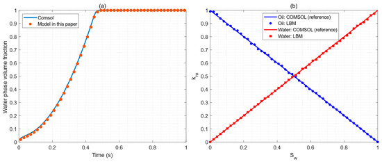
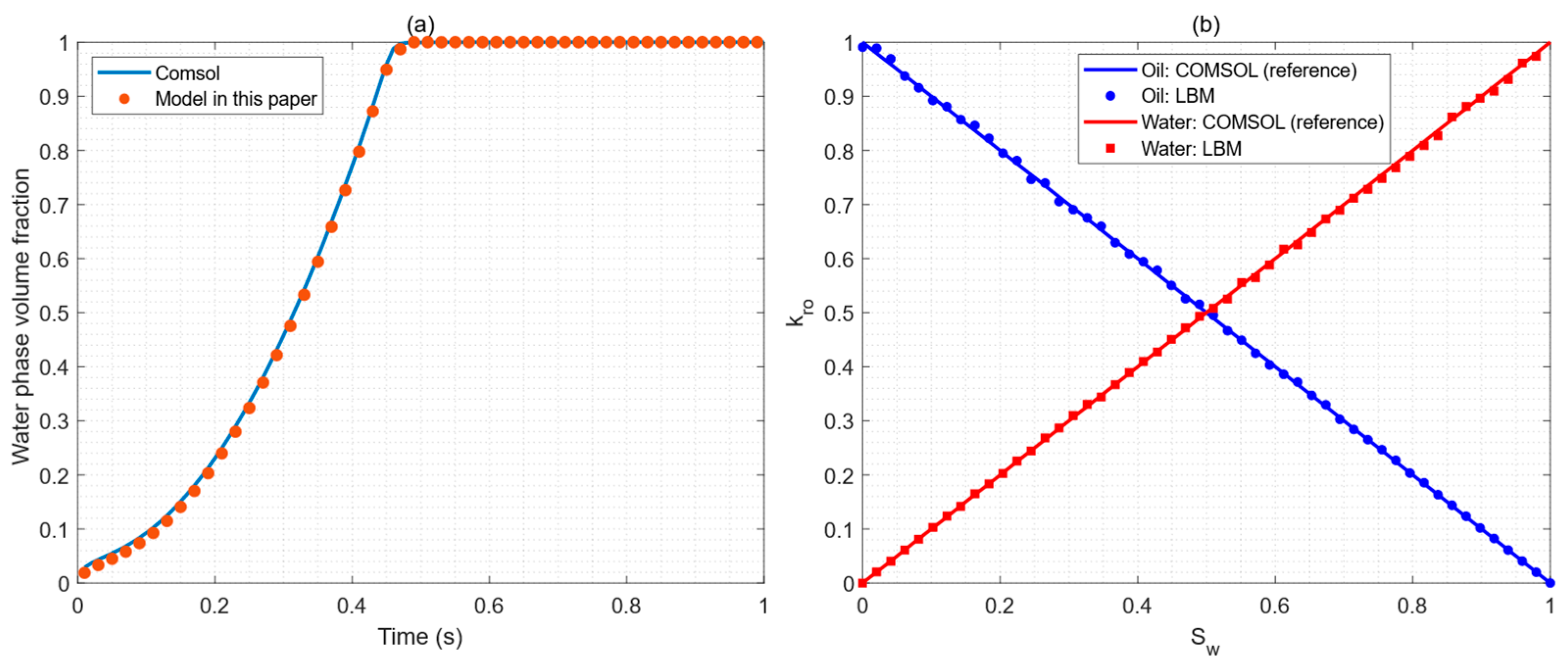
As a validation case for oil–water two-phase flow, this study simulates water displacing oil within a three-dimensional planar fracture. The fracture is represented as a rectangular domain with an aperture of 10 mm, width of 20 mm, and length of 100 mm. Initially saturated with oil, the fracture undergoes water injection at the inlet under a constant pressure gradient of 10 Pa. The present LBM model is employed to resolve the velocity fields and volume fractions of both phases during the displacement process. For comparative analysis, a counterpart simulation with identical geometry, initial conditions, and boundary conditions is implemented in COMSOL 6.1 using the level-set method. The temporal evolution of water volume fraction obtained from both approaches is systematically compared to validate the proposed numerical framework.

A comparative analysis of the aqueous-phase volume fraction at different temporal stages between the COMSOL simulation and the proposed model is presented in Figure 1. The results demonstrate close agreement between both methodologies, with a marginal relative error of 1.24%. This high level of consistency validates the reliability and accuracy of the developed oil–water two-phase flow model.

2.3. Simulation Strategy

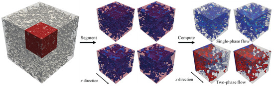
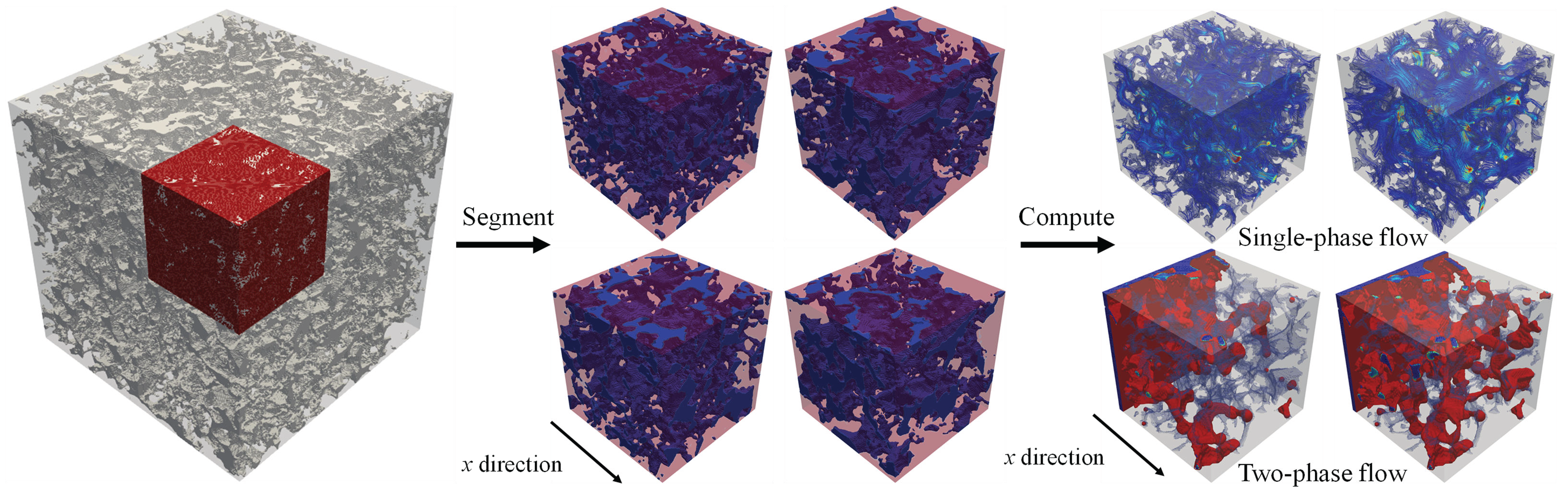
A core sample from the Ordos Chang-8 tight sandstone reservoir was selected and subjected to X-ray CT scanning to obtain three-dimensional digital images. The basis for selecting the permeability gradient of the seven digital cores is explained—the cores span a permeability range typical for the Ordos Chang-8 tight sandstone formation (from 0.01 mD to 5.0 mD). The grayscale CT images were subsequently binarized to reconstruct the pore-grain structure of the digital core. Given the substantial computational cost associated with the full-scale CT dataset for simulating two-phase flow, multiple representative sub-volumes were extracted using a sliding-window approach from the original scan data. Each extracted sub-volume measures 200 × 200 × 200 voxels, with a spatial resolution of 2 μm/voxel, corresponding to a physical dimension of 400 × 400 × 400 μm³. We computed porosity and permeability for sub-volumes of increasing size from 50³ to 300³ voxels and confirmed that the 200³ sub-volume falls within the stable plateau region in the performed representative elementary volume (REV) analysis. The numerical simulations were performed using a color-gradient lattice Boltzmann method (LBM) with MRT collision operator to enhance numerical stability. The computational domain was discretized into a regular cubic lattice (voxel grid) employing the D3Q19 velocity set. The time domain comprised 50,000 time steps, with steady-state flow conditions typically achieved by 30,000 steps. Boundary conditions were implemented as follows: velocity inlet using the Zou-He scheme, pressure outlet, and no-slip walls treated with the half-way bounce-back method. The above parameters were consistently applied in both case studies. To preserve the authentic pore-throat characteristics of the tight sandstone, no denoising procedures were applied, resulting in the retention of numerous isolated pores and disconnected flow pathways within the digital structures. A total of seven distinct digital sub-cores spanning a range of permeability values were ultimately selected for investigating oil–water two-phase flow through porous media. The entire workflow—from CT acquisition to sub-volume selection—is summarized in Figure 2.

The model configuration assigns the two faces normal to the x-direction as the fluid inlet and outlet, respectively, while the remaining four lateral surfaces are prescribed with periodic boundary conditions. To simulate two-phase flow through porous media, the initial phase distribution must be explicitly defined.

For homogeneous pressure distribution across the porous domain, 10-lattice-cell buffer zones are implemented at both ends along the x-direction. These buffers serve to impose constant-pressure boundary conditions for the water-flooding process. The left buffer is initialized with the aqueous phase, while the remainder of the domain—including the porous matrix and the opposite buffer—is saturated with the oil phase. The fluid viscosities are specified in lattice units as 0.1 for the oil phase and 0.01 for the aqueous phase, resulting in a viscosity ratio of 10:1 between the oil and water phases.

This study systematically simulates oil–water two-phase flow under 10 distinct pressure gradients across 7 digital rock cores with varying permeability values, supplemented by an additional investigation of a single core under 6 interfacial tension values and 10 pressure gradients. In total, 130 parameter combinations are simulated using a controlled-variable approach to elucidate the influencing factors and underlying mechanisms of sub-Darcy flow behavior. The porosity, permeability, and corresponding simulation schemes for all digital cores are summarized in

Table 1. Digital rock core parameters and simulation parameters (surface tension and pressure gradient are in lattice units).

No.	Porosity (Fraction)	Permeability (×10−3 μm2)	Surface Tension (Lattice Unit)	Pressure Gradient (Lattice Unit)
1	0.133	0.201	0.005–0.03	3 × 10−4~1 × 10−3
2	0.148	0.694	0.01
3	0.129	0.506
4	0.195	1.789
5	0.185	1.281
6	0.140	0.153
7	0.122	0.095

. All units of surface tension and pressure gradient are in lattice.

3. Simulation Results

3.1. LVND Flow in Tight Rocks

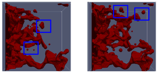
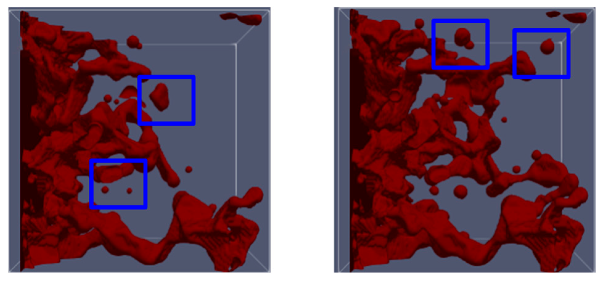
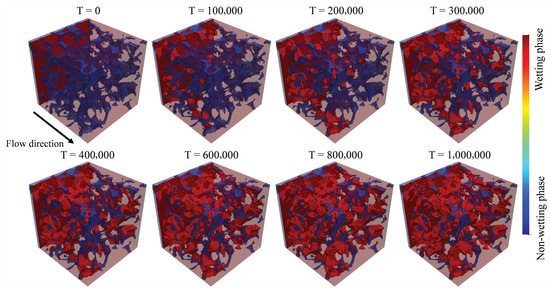
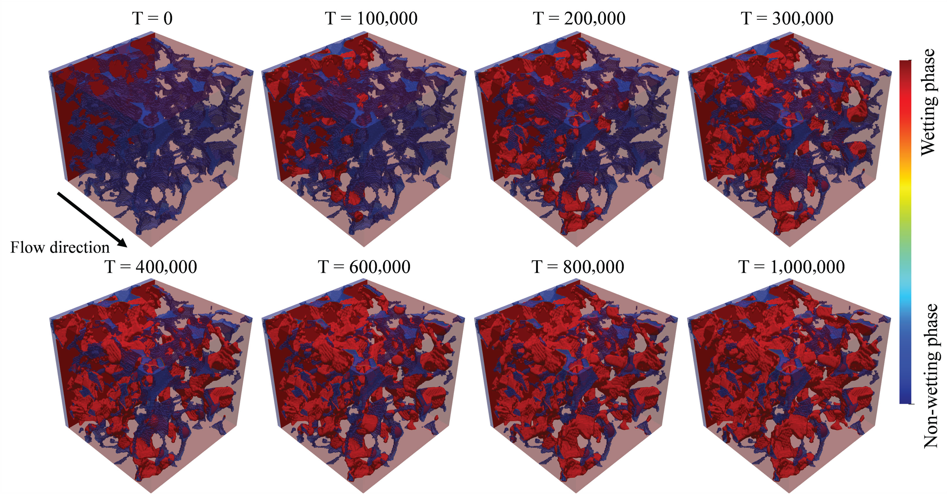
Figure 3 and Figure 4 illustrate the temporal evolution of phase distribution during the displacement process in Digital Core 1. Immiscible two-phase flow through porous media involves competitive interactions among capillary, viscous, and pressure gradient forces. Within this framework, capillary and viscous forces act as flow resistances, while the applied pressure gradient serves as the driving force.

Globally, the invading phase preferentially advances through high-permeability pathways, initially reaching the outlet via dominant flow channels. Subsequently, it gradually propagates through less conductive pores before eventual breakthrough. The displacement exhibits pronounced viscous fingering and snap-off phenomena. At low pressure gradients, viscous fingering dominates with negligible phase snap-off. Under these conditions, the combined effects of capillary pressure at oil–water interfaces and solid-fluid interactions generate substantial flow resistance. The limited driving force prevents aqueous-phase penetration through pore throats, resulting in stabilized menisci that remain stationary within constrictions.

With increasing pressure gradients, snap-off events emerge while fingering patterns become more extensive. Once the TPG is surpassed, the aqueous phase breaches throat constrictions and enters downstream pores. However, strong wall wettability prevents complete phase separation, leading to significant aqueous-phase retention along pore walls. The accumulated liquid in pore cavities subsequently refluxes into throats, ultimately triggering snap-off [37].

Notably, the presence of isolated pores and dead-end throats ensures persistent capillary effects throughout the displacement process, even after achieving stable water saturation. This is attributed to substantial irreducible water saturation retained within the core. Furthermore, pore geometry modulates the tripartite force balance: viscous fingering predominantly develops in larger pores where capillary thresholds are lower, whereas snap-off events concentrate in narrower throats and intensify with elevated pressure gradients.

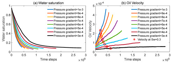
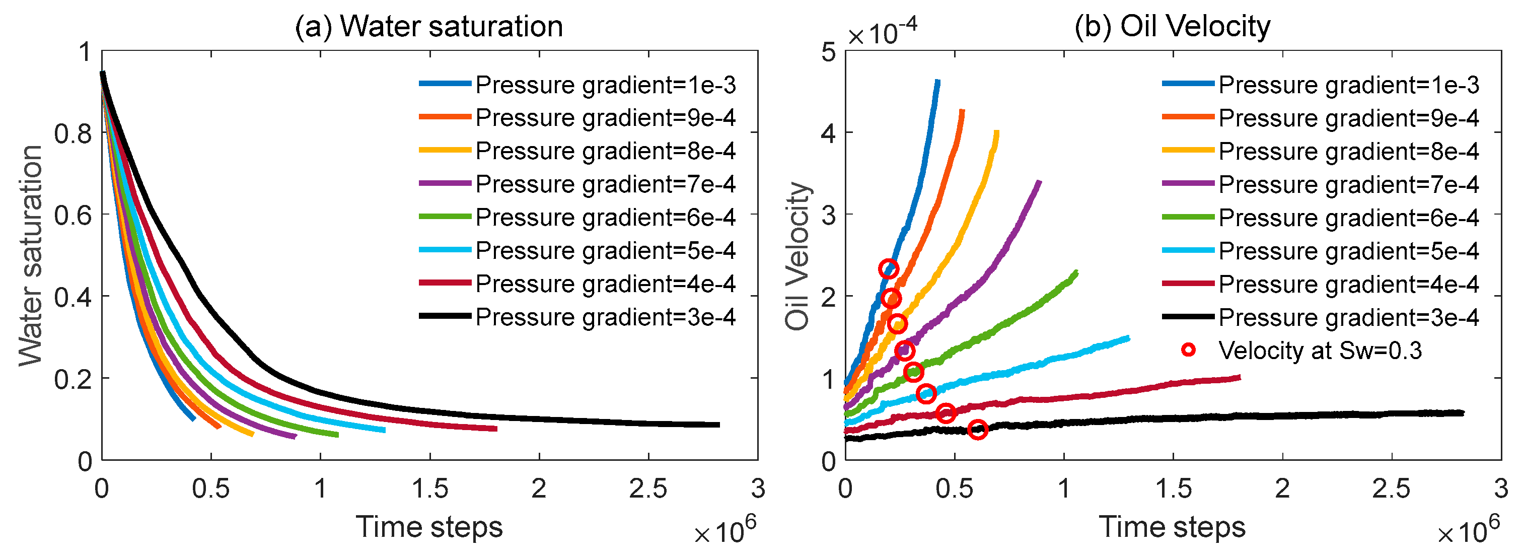
Owing to variations in pressure gradients, capillary forces, and pore-throat structures, the digital cores exhibit divergent stabilization times and residual water saturations. To establish a unified comparative framework, this study adopts the outlet velocity at a uniform water saturation of 0.3 as the representative flow velocity for each pressure gradient. This standardized metric enables systematic investigation of the relationship between pressure gradient and oil-phase velocity, thereby elucidating sub-Darcy flow characteristics in porous media. The scatter points in Figure 5b correspond to these representative velocities measured at water saturation of 0.3 across all applied pressure gradients.

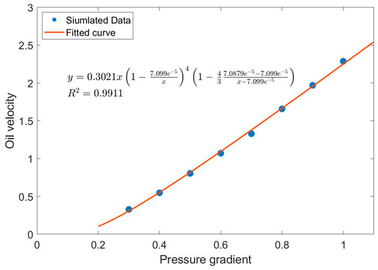
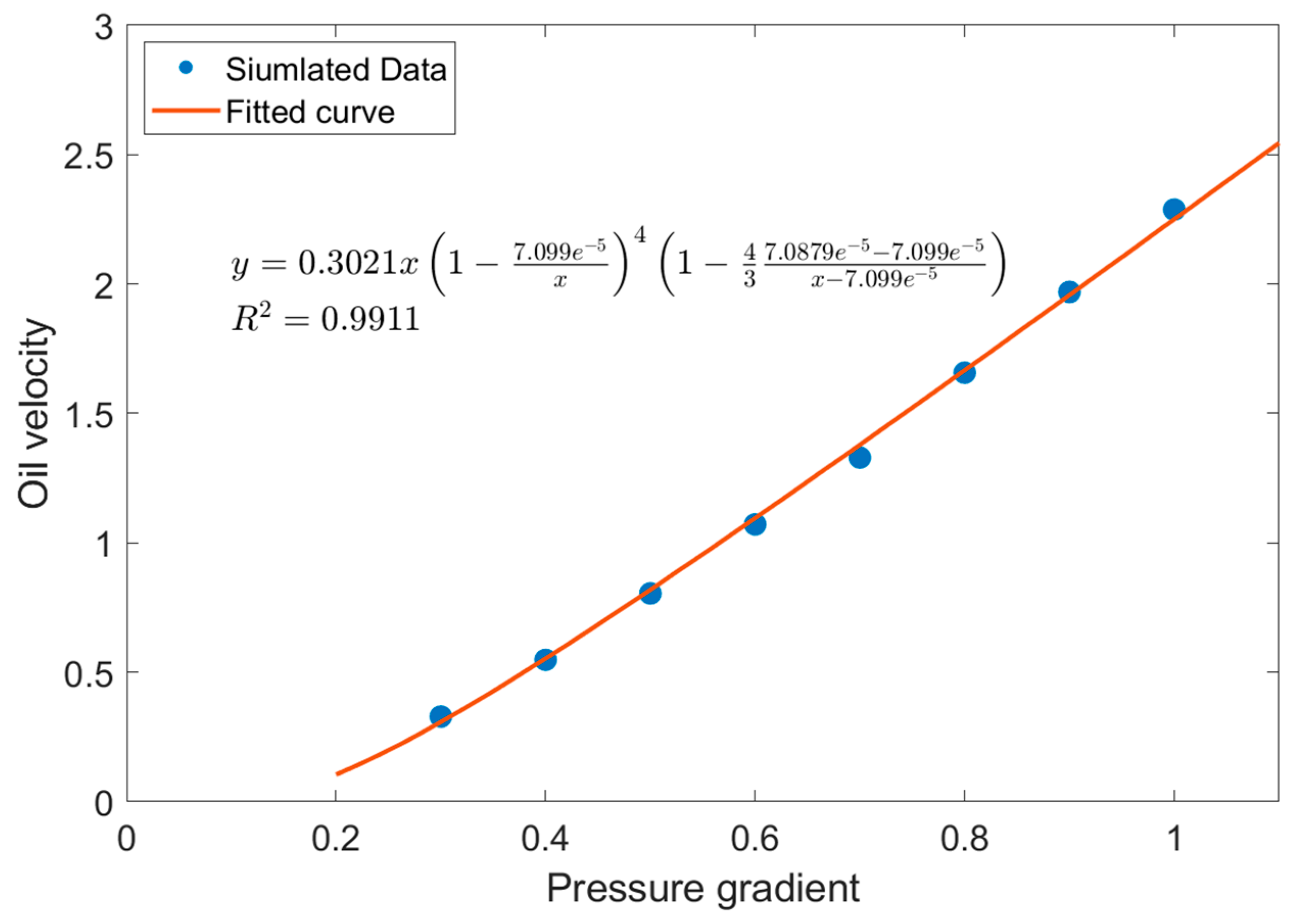
Figure 6 illustrates the relationship between applied pressure gradients and corresponding flow velocities. The results reveal a characteristic nonlinear correlation that does not pass through the origin, demonstrating distinct TPG behavior and sub-Darcy flow phenomena. The pressure gradient–velocity profile can be delineated into three sequential regimes. TPG regime: At low pressure gradients, the driving force remains insufficient to overcome the combined resistance from capillary and viscous forces, resulting in negligible flow. Nonlinear flow regime: Once the pressure gradient exceeds the cumulative resistance, flow initiation occurs. However, the comparable magnitude between driving and resistant forces renders capillary-induced energy dissipation non-negligible, producing marked nonlinearity. Linear flow regime: With further increase in pressure gradient, the relative influence of capillary and viscous forces diminishes, leading to a gradual transition toward a linear pressure gradient–velocity relationship. This tripartite flow behavior can be quantitatively characterized by a two-parameter equation incorporating the TPG (λ) and a boundary-layer parameter (δ).

3.2. Effect of Capillary Force

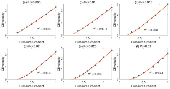
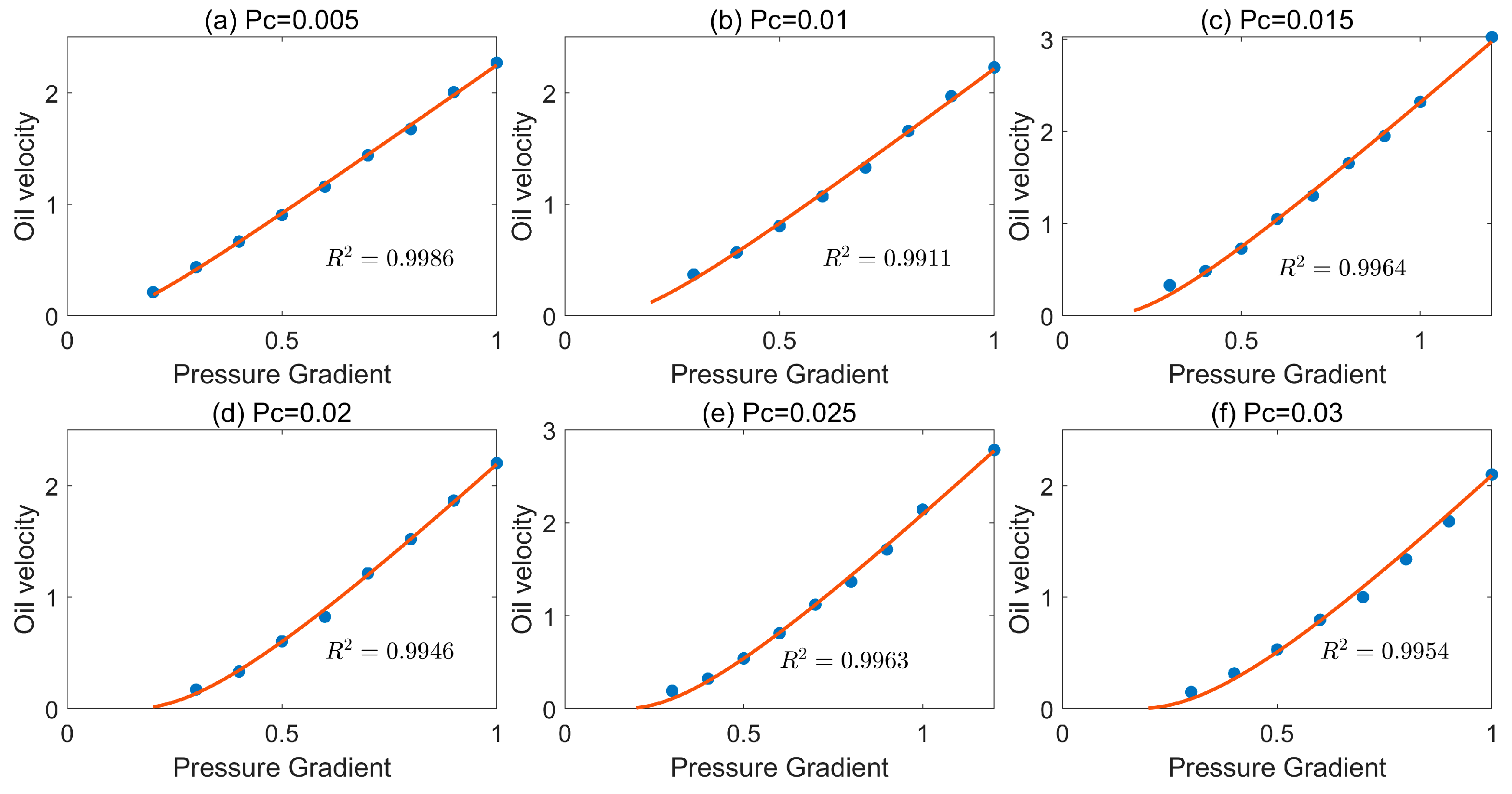
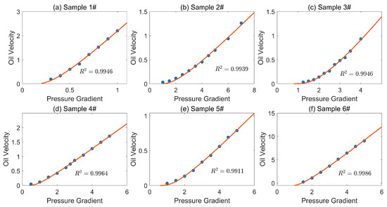
Capillary forces primarily augment the frictional resistance between non-wetting phases and pore walls. While often negligible in coarse-grained porous media, these forces become significant in tight formations where non-wetting-phase mobilization requires the driving force to overcome both capillary barriers and frictional resistance. Tight sandstone reservoirs typically contain clay minerals whose distinct mineralogical compositions yield varying capillary characteristics. Figure 7 demonstrates the evolution of sub-Darcy flow curves for core 1 as capillary pressure increases from 0.005 to 0.03. At lower capillary pressures, the nonlinearity of the flow curve is subdued, approaching an almost linear pressure–velocity relationship, though the TPG effect remains pronounced. Reduced capillary pressure diminishes flow resistance in boundary layers, enabling fluid movement under lower pressure differentials. With increasing capillary pressure, the TPG shows minimal enhancement, whereas the nonlinearity of the flow curve intensifies significantly. This indicates that elevated capillary forces predominantly amplify flow nonlinearity rather than substantially raising the initiation threshold.

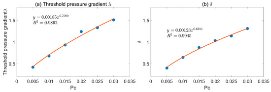
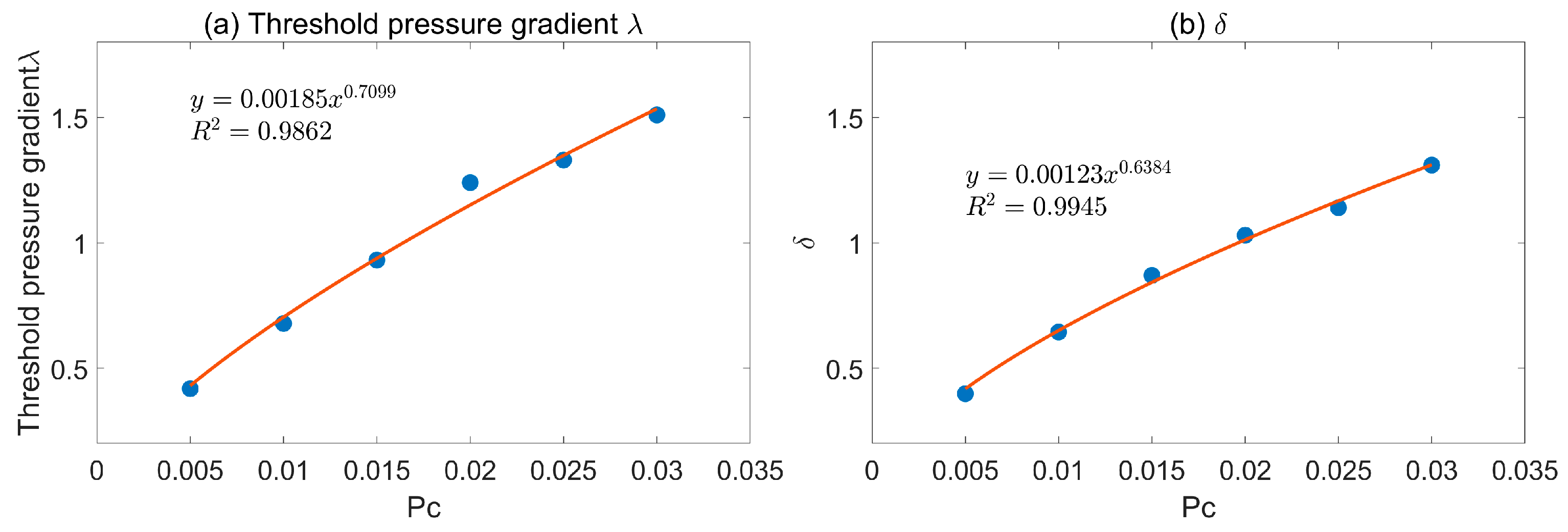
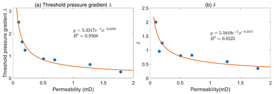
The pressure gradient and velocity relationships under different capillary forces were fitted by Formula (21), and the starting pressure gradient λ and nonlinear parameter δ under each capillary force were obtained. Figure 8 shows the capillary force and the relationship between λ and δ, both of which increase with the increase in capillary force. The capillary force and the relationship between λ and δ can both be expressed by power functions. The relationship between the starting pressure gradient λ and the capillary force is: $\lambda =0.00185{p_c}^{0.7099}$; the relationship between the nonlinear parameter δ and the capillary force is: $\delta =0.00123{p_c}^{0.6384}$.

3.3. Effect of Viscosity

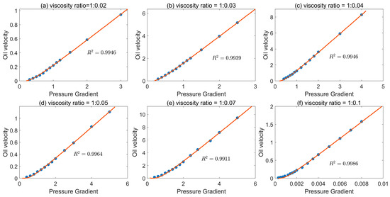
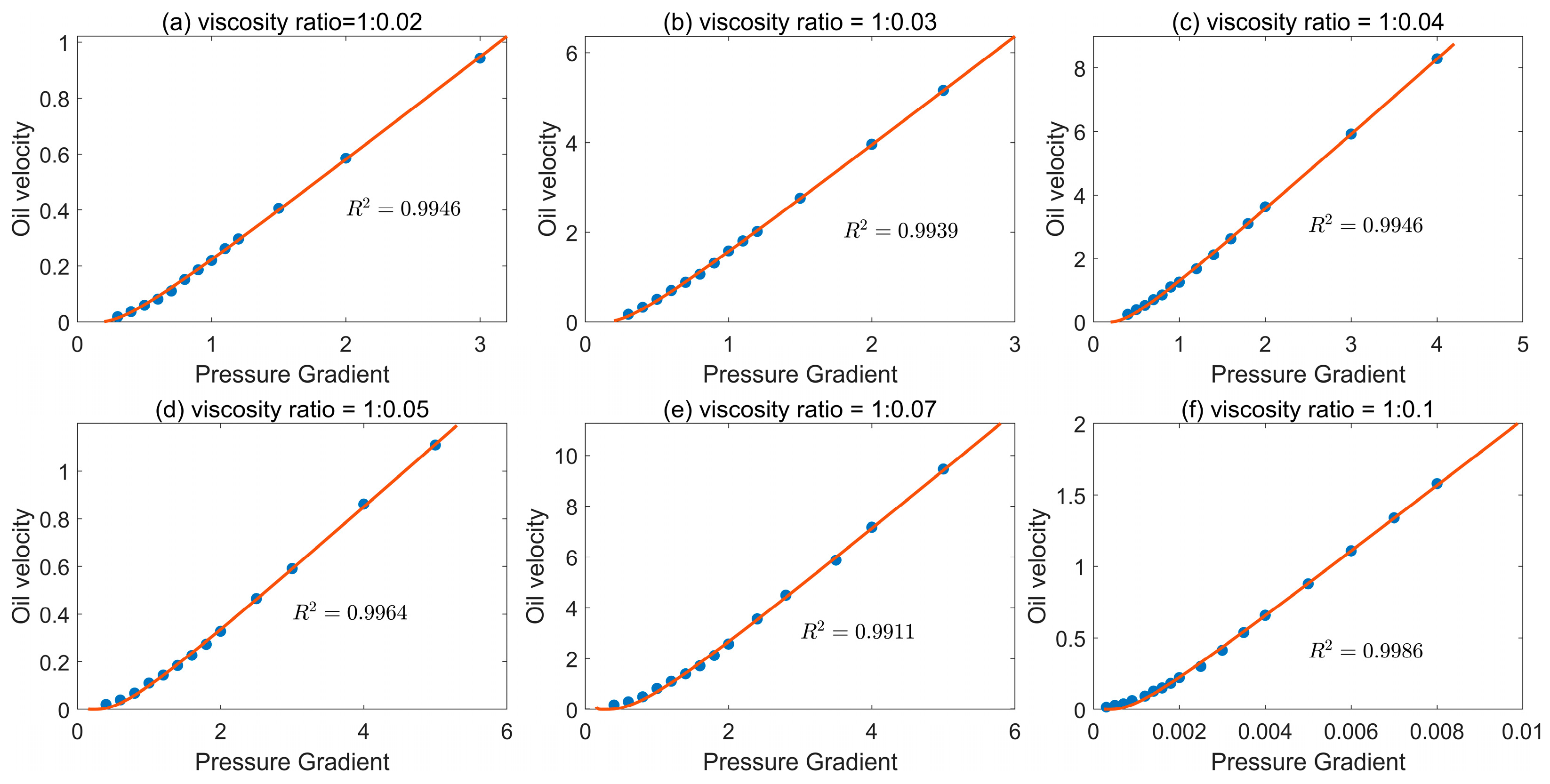
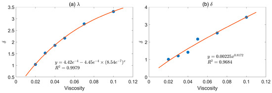
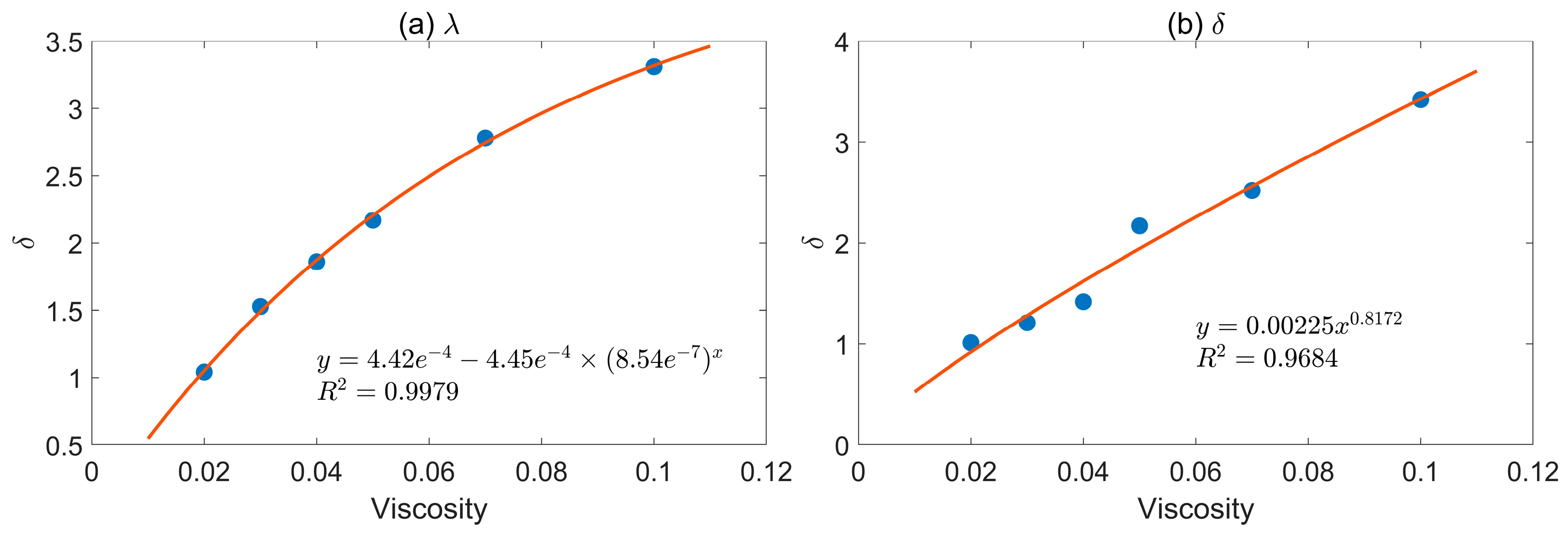
Figure 9 and Figure 10 illustrate the influence of viscosity ratio on sub-Darcy flow behavior. During bi-phasic flow through porous media, elevated viscosity of the immiscible phase enhances inter-phase viscous forces, promoting flow homogenization. Increased viscosity amplifies internal fluid friction, thereby augmenting flow resistance. This heightened resistance necessitates greater pressure gradients to sustain flow, exacerbating the manifestation of sub-Darcy phenomena. Furthermore, viscosity modulates boundary-layer development. Higher-viscosity fluids develop thicker boundary layers, which subsequently alter velocity profiles and pressure distributions, ultimately modifying macroscopic flow characteristics.

3.4. Effect of Permeability

The inherent pore structure and spatial heterogeneity of porous media fundamentally govern fluid pathways, thereby shaping the manifestation and evolution of sub-Darcy flow. Tight porous systems exhibit particularly complex pore-throat configurations that resist accurate parametrization. While permeability—representing the macroscopic flow capacity at the REV scale—provides an indirect measure of geometric complexity, it serves as a practical metric for comparative analysis.

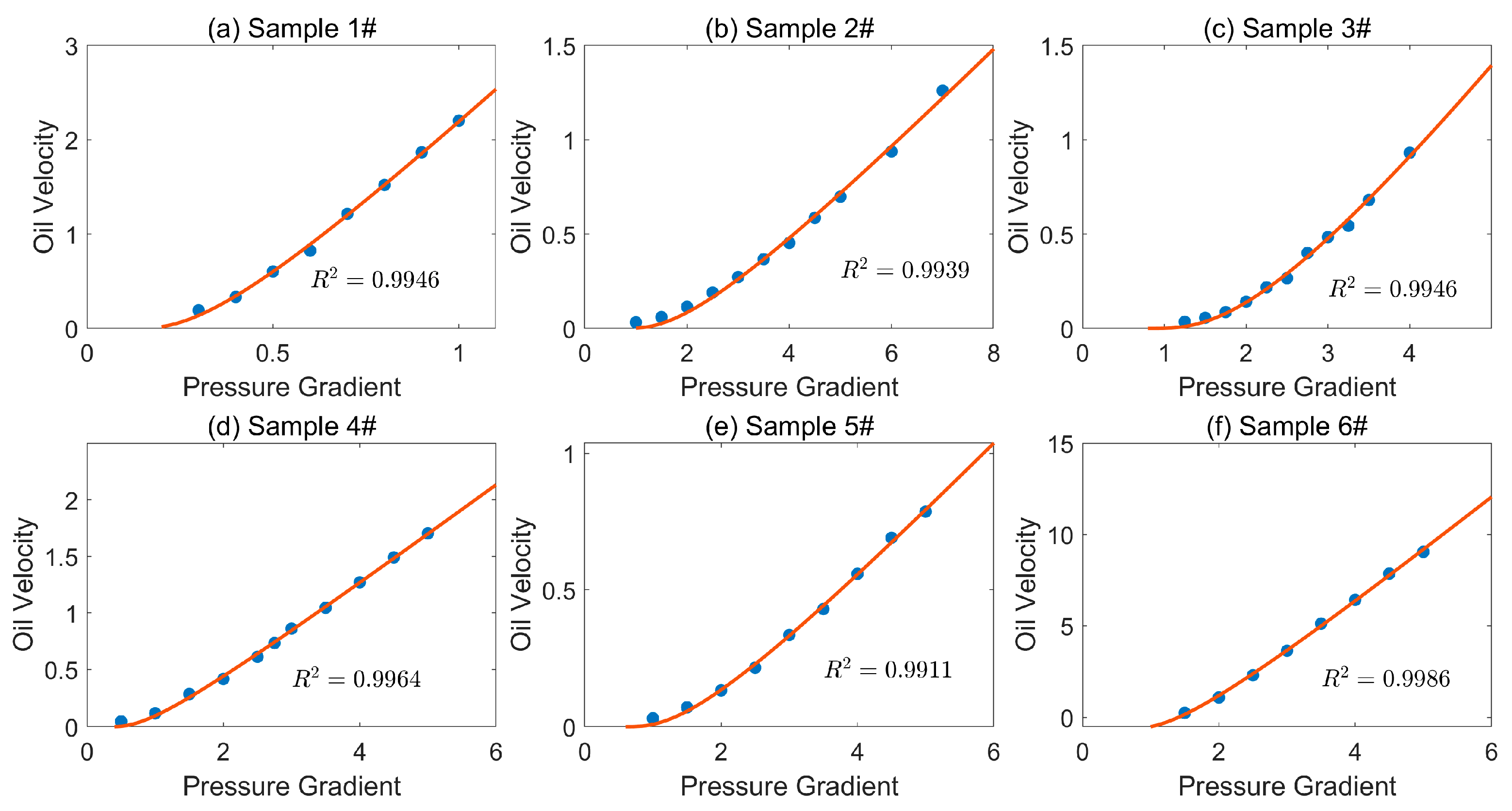
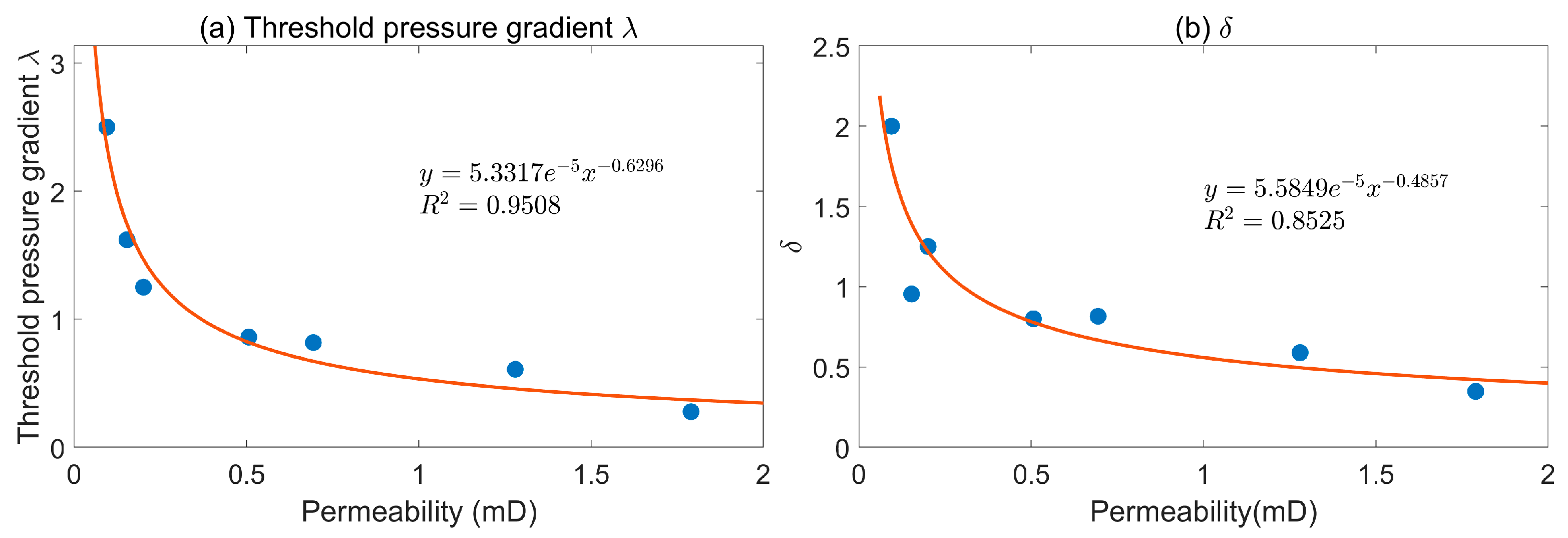
This study investigates permeability-dependent sub-Darcy behavior using cores spanning a range of permeability values, as summarized in Figure 11 and Figure 12. The results establish that lower permeability correlates strongly with elevated TPG s and enhanced flow nonlinearity, demonstrating the critical role of pore-scale architecture in modulating non-Darcy flow dynamics.

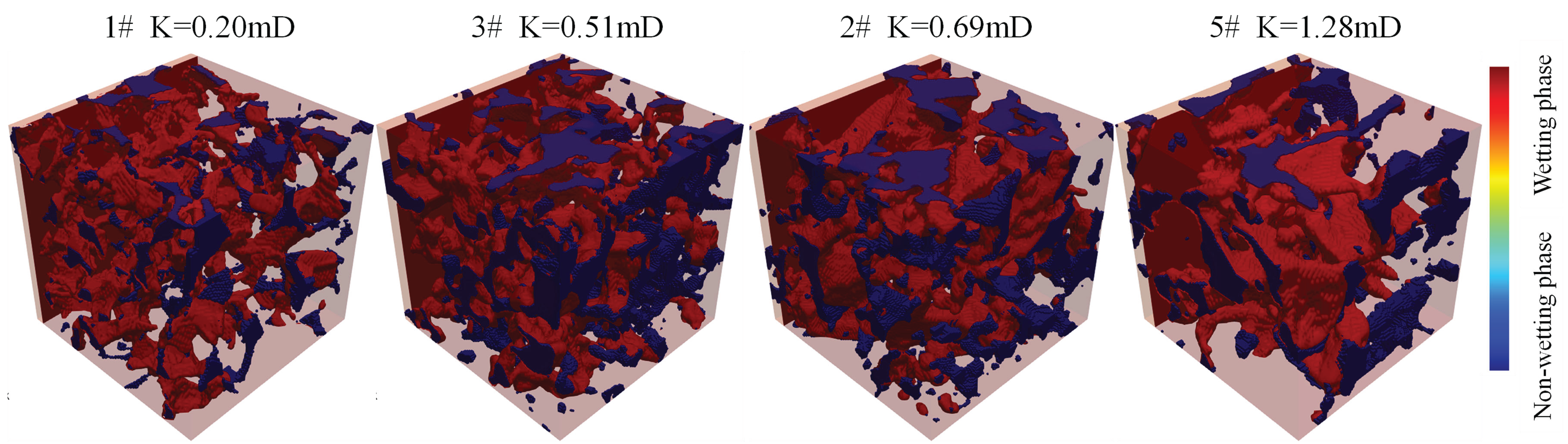
Figure 13 presents the oil–water phase distributions at a uniform water saturation of 0.3 across cores with varying permeability values. The results demonstrate that decreasing permeability is associated with progressively more complex pore-throat architectures. Although all cores maintain identical water saturation, lower-permeability specimens exhibit increasingly heterogeneous aqueous-phase distribution. This spatial heterogeneity amplifies the capillary resistance that must be overcome during flow, establishing an inverse relationship between permeability and effective capillary barriers. Consequently, diminished permeability correlates with reduced oil-phase velocity at the outlet, reflecting the compounded effects of structural complexity and capillary dominance.

Both parameters exhibit a decreasing trend with increasing permeability, following a negative power-law relationship. The TPG correlates with permeability as $\lambda =5.3317e^{-5}{k}^{-0.6296}$. The nonlinear parameter δ varies with permeability as $\delta =5.5849e^{-5}{k}^{-0.4857}$. In tight reservoirs, reduced permeability corresponds to narrower pore throats and higher specific surface area. This geometric configuration intensifies boundary-layer effects and amplifies solid–fluid and fluid–fluid interactions, thereby elevating capillary resistance against oil-phase movement. The resultant flow impedance manifests as an enhanced TPG and pronounced nonlinear flow behavior.

4. Discussion

4.1. The Low-Velocity Non-Darcy Flow Model

Based on the experimental investigation of sub-Darcy flow and the preceding pore-scale numerical simulations, the existence of sub-Darcy flow phenomena in tight sandstones and their governing mechanisms have been unequivocally established. Both experimental and computational results demonstrate that sub-Darcy flow behavior in tight sandstones can be quantitatively described by the following two-parameter equation:

$$v=\left\{\begin{array}{cc}0,& \nabla p\le \lambda \\ -{\displaystyle \frac{k}{\mu }}\nabla p{\left(1-{\displaystyle \frac{\lambda }{\nabla p}}\right)}^4\left(1-{\displaystyle \frac{4}{3}}{\displaystyle \frac{\delta -\lambda }{\nabla p-\lambda }}\right),& \nabla p>\lambda \end{array}\right.$$

(22)

In the formula: $k$ represents permeability, m²; $\mu$ represents fluid viscosity, Pa·s; $\nabla p$ represents pressure gradient, Pa/m; The δ is a parameter for controlling the nonlinearity degree of the LVND flow, Pa/m; $\lambda$ is used to initiate the pressure gradient, Pa/m.

In Equation (22), δ is a nonlinear exponent that characterizes the curvature of the flow velocity versus pressure gradient relationship, and it is quantitatively correlated with the pore-throat size distribution and the boundary-layer thickness. A narrower pore-throat distribution, which corresponds to a higher sorting coefficient, yields a smaller δ, approaching linear flow. Conversely, a wider pore-throat distribution yields a larger δ, resulting in more pronounced nonlinearity. The threshold pressure gradient, denoted as λ, refers to the minimum pressure gradient required for a fluid to initiate macroscopic flow in ultra-low-permeability porous media, reflecting solid–liquid interfacial interactions and pore-throat bottleneck effects. A larger λ indicates lower permeability, finer pore throats, and thicker boundary layers. As a result, the region of “dead oil” or “bound fluid” that cannot be mobilized under conventional production pressure differentials becomes larger, water flooding requires a greater pressure differential, recoverable reserves decrease, and development difficulty increases. Conversely, a smaller λ indicates flow closer to Darcy flow and better medium homogeneity.

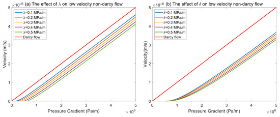
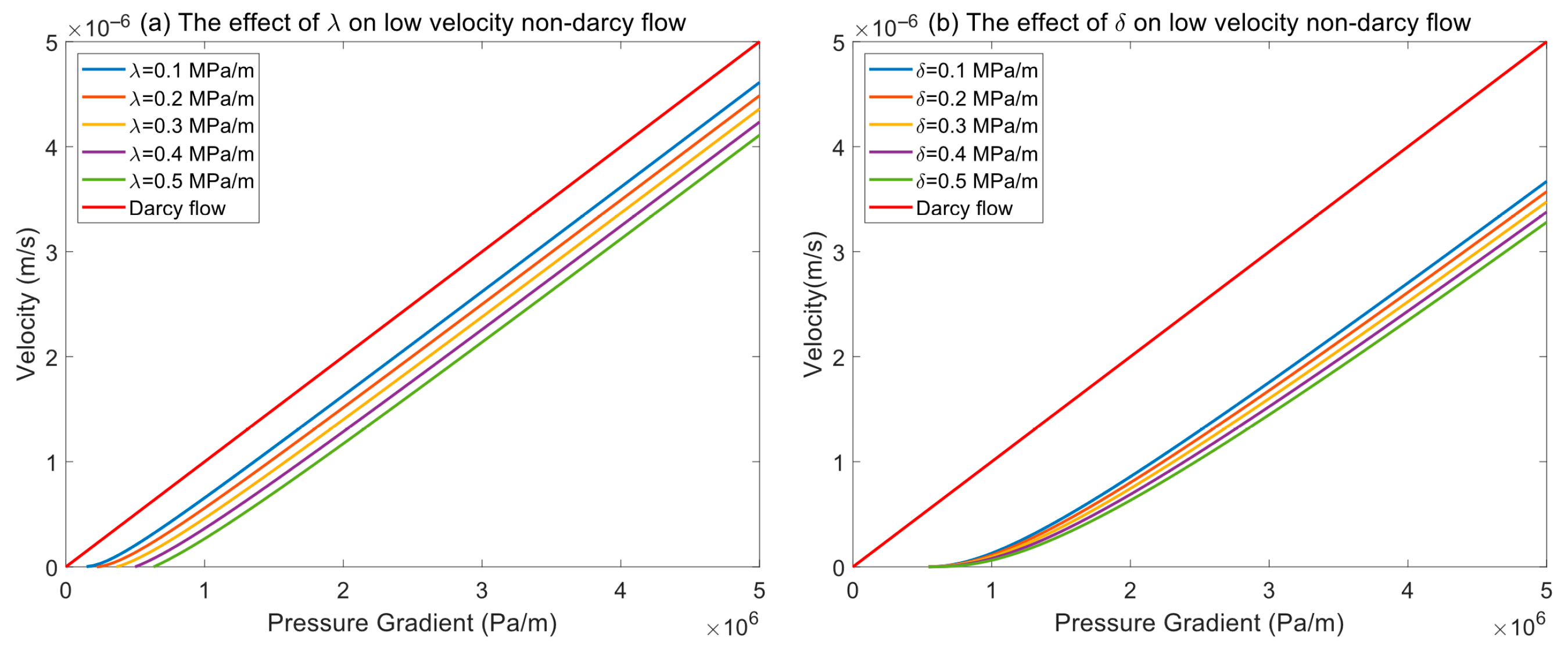
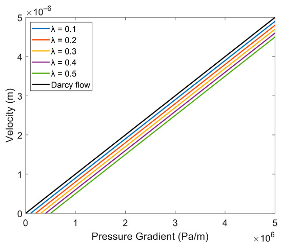
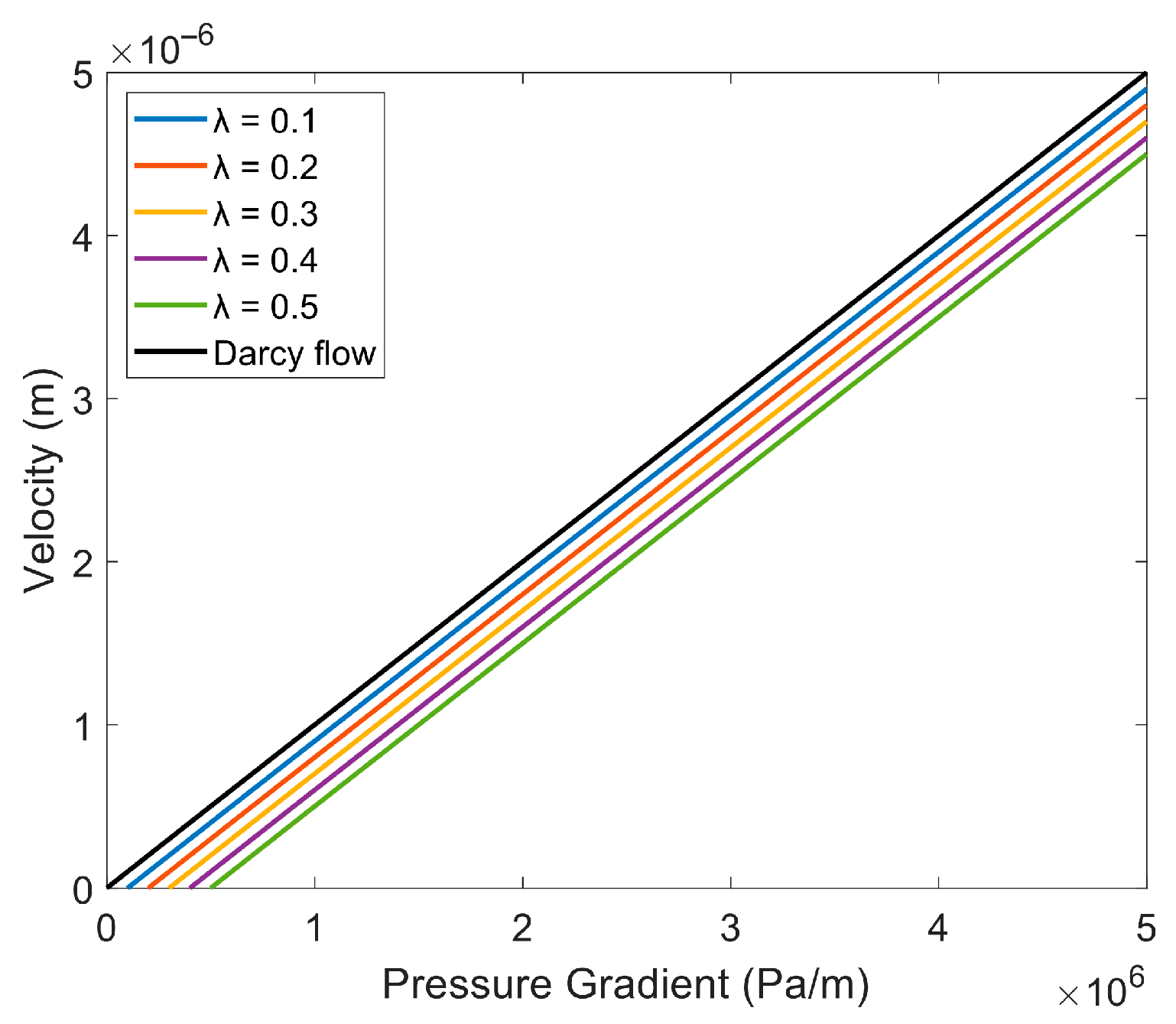
Figure 14 shows the influence of different λ and δ values on the LVND flow effect when the permeability is 0.1 × 10⁻³ μm² and the viscosity is 1 × 10⁻³ Pa·s. When δ is constant, the larger λ is, the greater the pressure gradient required for the fluid to undergo LVND flow. When λ is constant, the larger δ is, the stronger the nonlinearity of LVND flow will be. Therefore, λ controls the beginning of non-Darcy flow, δ controls the degree to which non-Darcy flow deviates from Darcy flow, and both jointly control the intensity of non-Darcy flow.

4.2. Comparison with Other Models

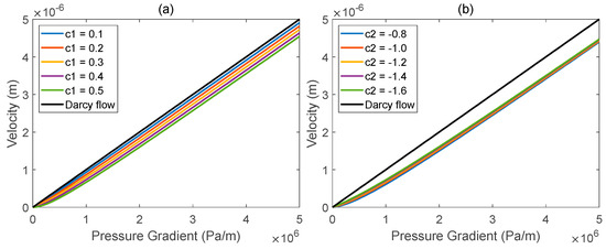
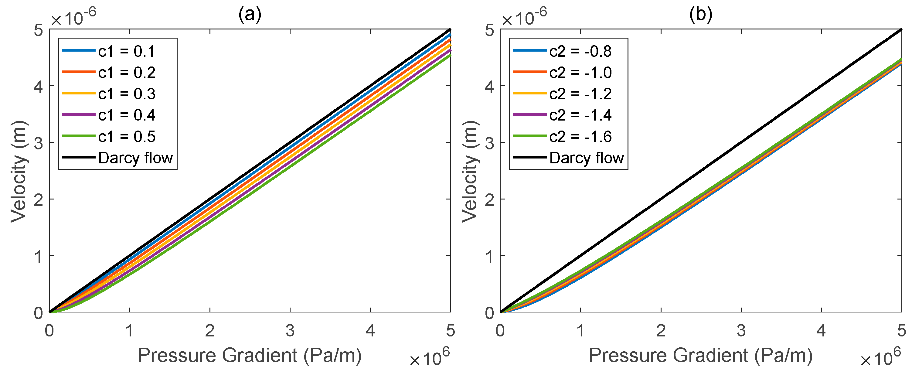
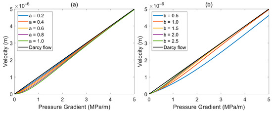
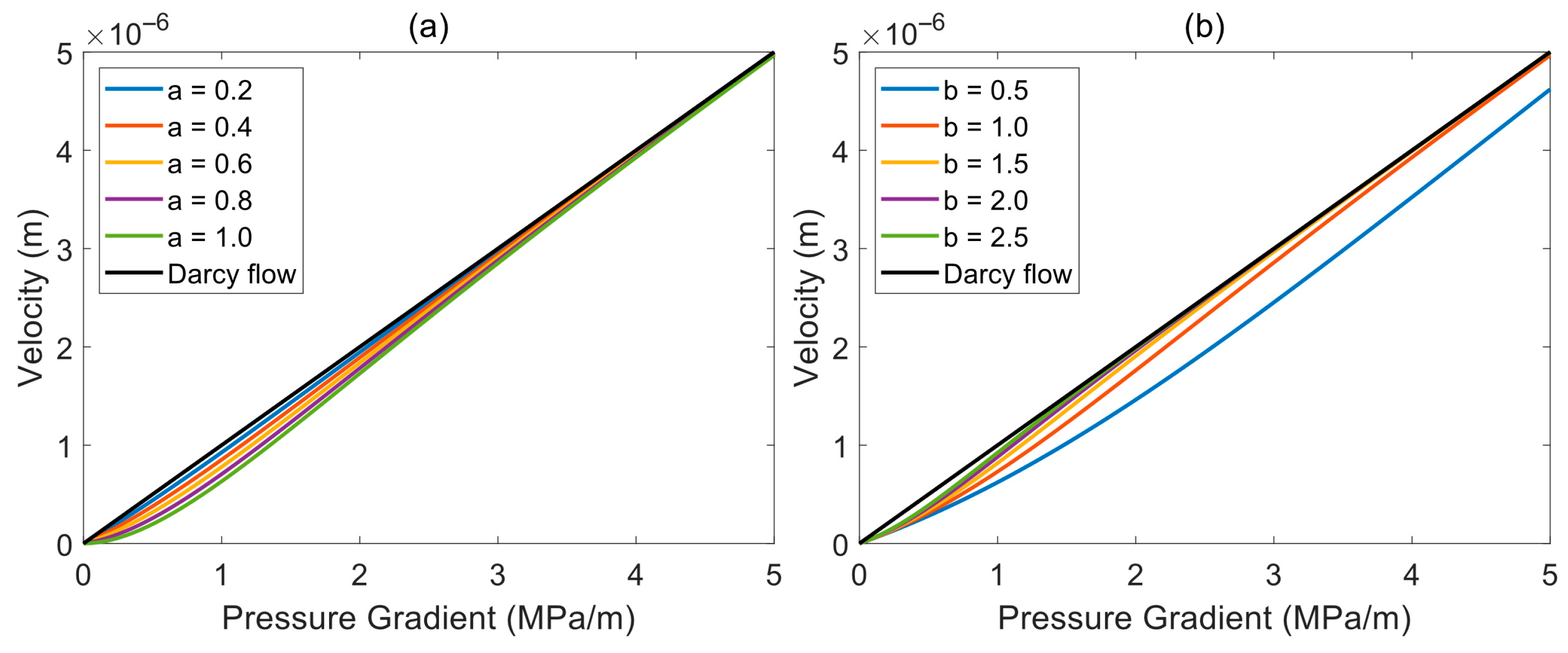
To further validate the effectiveness and superiority of the model proposed in this paper, it is compared against three typical LVND models found in the literature—specifically, the models presented in references [6,15,22], which have been listed in

Table 2. Comparison of different LVND models.

References	Equation	Parameters
[6]	$v={\displaystyle \frac{k}{\mu }}\left(1-{\displaystyle \frac{\lambda }{\left|\nabla p\right|}}\right)\cdot \nabla p$	λ is the TPG.
[15]	$v=-{\displaystyle \frac{k}{\mu }}\left(1-{\displaystyle \frac{c_1}{\nabla p-c_2}}\right)\cdot \nabla p$	c1 and c2 are characteristic parameters for the TPG and nonlinear flow.
[22]	$v=-{\displaystyle \frac{k}{\mu }}\left(1-a\cdot \exp \left(-b\cdot \left|\nabla p\right|\right)\right)\cdot \nabla p$	a and b are coefficients of nonlinear flow equation.

. Figure 15, Figure 16 and Figure 17 illustrate the LVND curves generated by the models in the references, respectively. In comparison, the model in reference [6] is capable of describing only the flow characteristics associated with a threshold pressure gradient; it lacks sufficient precision in characterizing nonlinear flow behavior within the low-velocity regime. The model in reference [15] introduces two characteristic parameters, c₁ and c₂, which to some extent enhance its capacity to describe nonlinearities; however, it fails to capture the characteristics associated with a threshold pressure gradient. The model in reference [22] employs a dual-coefficient nonlinear equation; while its mathematical form is relatively complex, it lacks a clear physical articulation of the underlying mechanism governing the threshold pressure gradient. Furthermore, as the pressure gradient increases, the velocity curve generated by this model gradually converges toward Darcy flow behavior. Additionally, the influence of parameter *b* on the model’s output remains ambiguous, rendering it incapable of accurately characterizing the specific features of low-velocity non-Darcy flow. A comprehensive comparative analysis reveals that the model proposed in this paper not only surpasses the benchmark models in terms of fitting accuracy but also features parameters endowed with clear physical significance, thereby enabling a more comprehensive reflection of both the initiation characteristics and the nonlinear evolutionary processes inherent to LVND flow. Moreover, the proposed model demonstrates excellent adaptability to flow behaviors occurring under diverse pore structures, fluid properties, and pressure conditions, suggesting broad prospects for practical engineering applications. Consequently, the model presented in this paper exhibits significant advantages in the description of low-velocity non-Darcy flow.

5. Application

5.1. Case 1: Depletion Production of Fractured Horizontal Well

To elucidate the distinction between Darcy and non-Darcy flow effects on production performance, we implemented an EDFM [11,38] to simulate well production dynamics in an ultra-low-permeability reservoir under two constitutive relationships: classical Darcy flow and the experimentally validated non-Darcy flow (Equation (21)). The boundary and initial conditions adopted in the model are shown in

Table 3. The boundary and initial conditions for case 1.

Parameter	Value
Reservoir boundary	Closed
Initial reservoir pressure	20 MPa
Porosity	0.1
Matrix permeability	0.5 mD
Initial water saturation	0.4
Bottom-hole flowing pressure	10 MPa
Horizontal well length	800 m
Number of hydraulic fractures	12
Fracture half-length	120 m
Fracture conductivity	10 D·cm
Fluid viscosity	5.0 mPa·s
Threshold pressure gradient	0.05 MPa/m

.

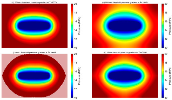
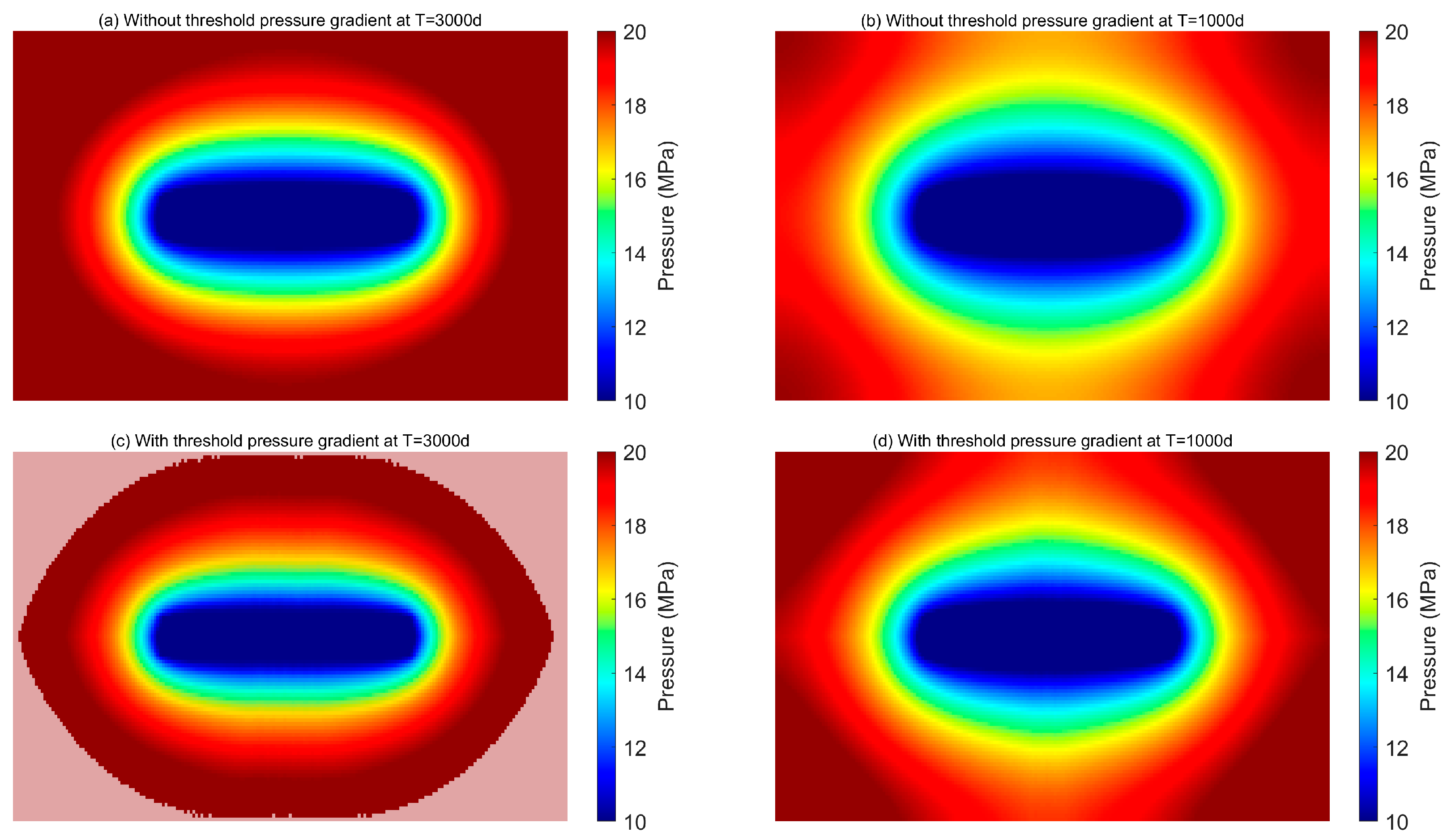
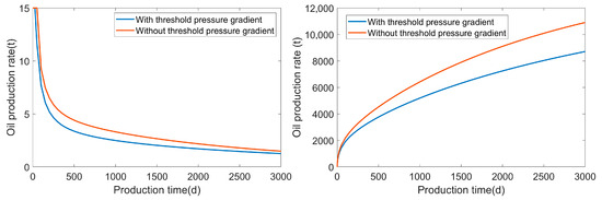
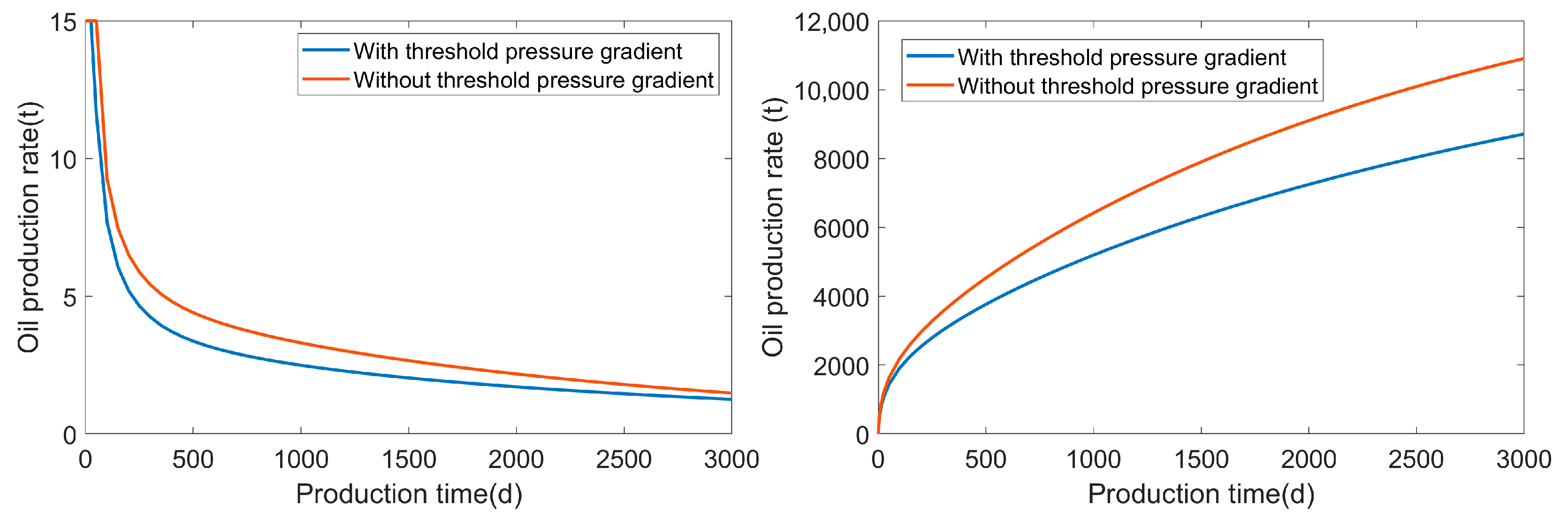
According to Darcy’s law, fluid movement occurs throughout the reservoir wherever a pressure differential exists between injector and producer, albeit at varying rates. However, by neglecting threshold resistance mechanisms, the Darcy formulation overestimates production rates. In contrast, the non-Darcy model predicts significantly reduced productivity, aligning with field-observed challenges of “ineffective injection and limited production”.

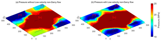
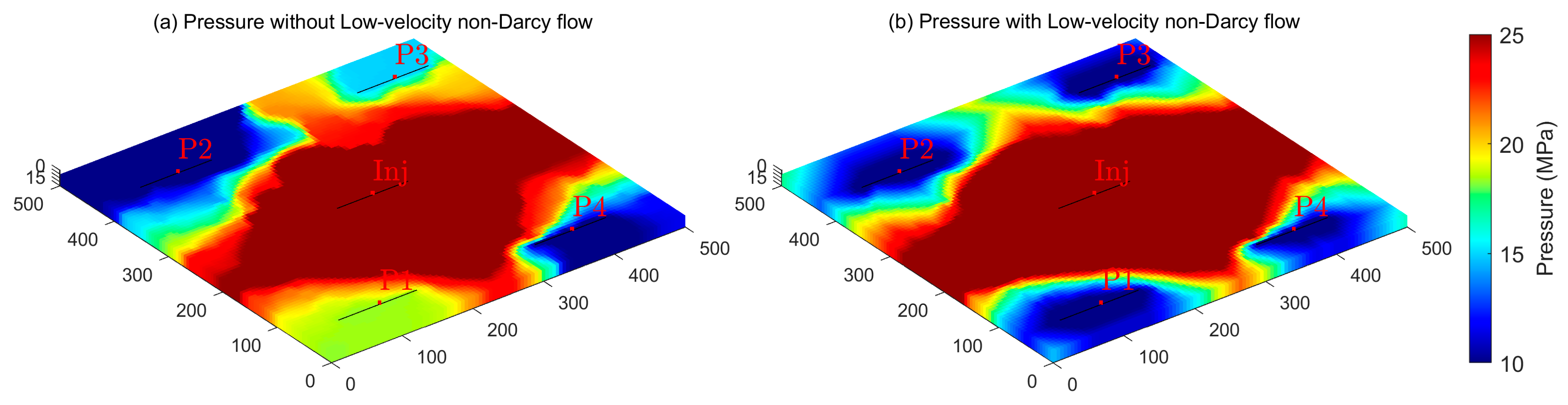
Comparative simulations of depletion development under both flow regimes (Figure 18 and Figure 19) reveal substantial impacts of sub-Darcy flow on ultra-tight reservoir performance. Relative to Darcy flow predictions, the non-Darcy model reduces initial production rates by 28.4% and decreases estimated ultimate recovery by 20.12%, demonstrating the critical importance of accurate flow characterization for realistic production forecasting.

5.2. Case 2: Water Injection of Fractured Vertical Wells

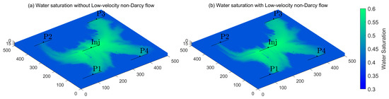
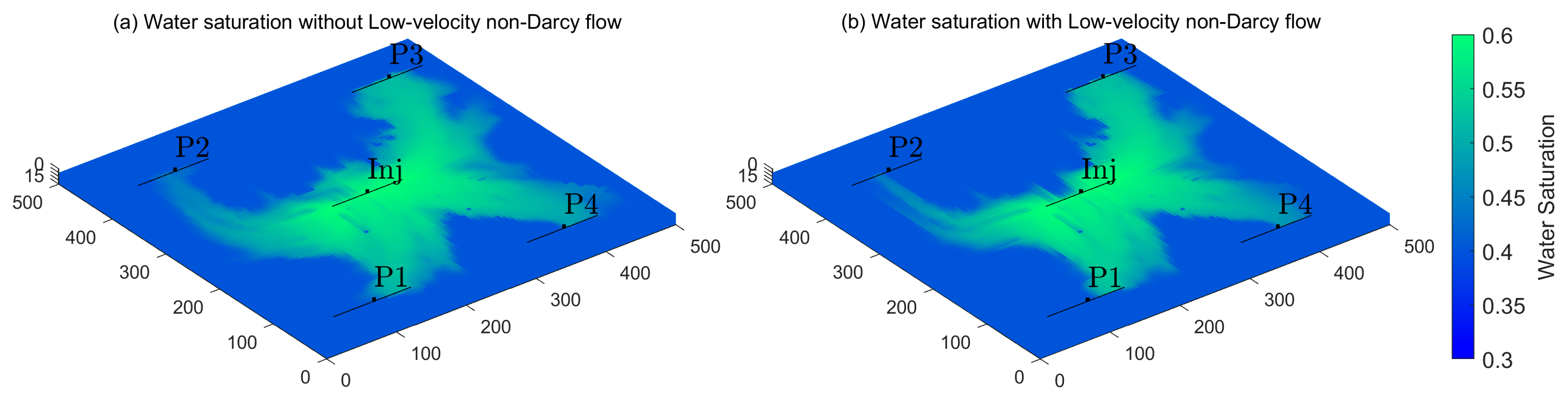
Furthermore, water-flooding performance in the ultra-low-permeability reservoir was simulated under the sub-Darcy flow regime, with results presented in Figure 14 and Figure 15. Compared to the Darcy flow scenario, reservoir regions experiencing pressure gradients below the threshold gradient—particularly areas distant from wellbores with minimal injection–production pressure differentials—exhibit complete flow stagnation, forming “dead oil zones” or “non-flow domains.” This fundamentally alters streamline patterns, effectively narrowing the available flow pathways. The boundary and initial conditions adopted in the model are shown in

Table 4. The boundary and initial conditions for case 2.

Parameter	Value
Reservoir boundary	Closed
Initial reservoir pressure	20 MPa
Initial water saturation	0.4
Injection well bottom-hole pressure	25 MPa
Production well bottom-hole pressure	10 MPa
Well spacing	300 m
Fracture half-length	100 m
Fracture conductivity	5 D·cm
Matrix permeability	0.1 mD
Porosity	0.1
Water viscosity	1 mPa·s
Oil viscosity	5.0 mPa·s
Threshold pressure gradient	0.05 MPa/m

.

As the injected water front propagates outward, its energy dissipates rapidly due to the TPG, resulting in significantly reduced sweep efficiency compared to Darcy-based predictions under identical injection pressures and timeframes, which is shown in Figure 20 and Figure 21. To mobilize crude oil in these formations, injectors must supply additional pressure to overcome the threshold gradient. Consequently, the simulations demonstrate requirement for elevated bottom-hole flowing pressure to initiate and maintain target injection rates.

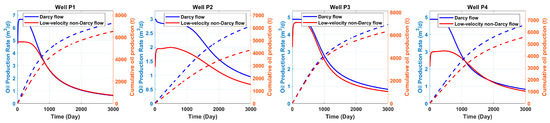
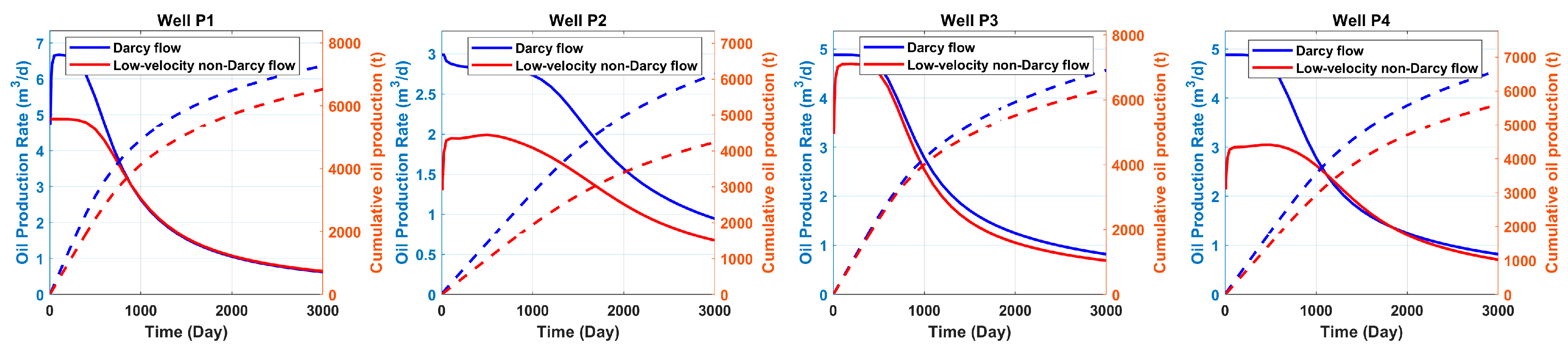
Figure 22 compares production profiles under Darcy and sub-Darcy flow regimes across multiple wells. Due to the constrained drainage radius—effectively “locked” by threshold gradient effects—the accessible geologic reserves become finite and fixed. As depletion progresses, the average pressure within the drainage domain declines continuously, causing the bottom-hole flowing pressure to reach technical or economic limits more rapidly. Consequently, wells operating under sub-Darcy conditions cannot sustain plateau production and enter the decline phase earlier than predicted by Darcy flow models. This premature decline, combined with reduced drainage efficiency, results in significantly lower cumulative oil production compared to conventional Darcy-based forecasts.

6. Limitations and Future Work

Despite the improved understanding of low-velocity non-Darcy flow provided by this pore-scale study, several limitations should be acknowledged. First, all simulations are performed in lattice units without conversion to physical units, which prevents direct quantitative validation against specific experimental cores. Second, grid-sensitivity and voxelization artifacts have not been systematically quantified. Third, wettability is assumed to be homogeneous and constant, neglecting dynamic contact-angle effects. Fourth, the pore-scale reconstruction involves segmentation uncertainties that may affect the extracted parameters λ and δ. Fifth, the current analysis does not employ the capillary number (Ca = μv/σ) to unify the description of flow regimes. Consequently, the transition between capillary-dominated, transitional, and viscous-dominated flows has not been quantitatively delineated [39,40].

Future work will focus on: (i) calibrating lattice-to-physical unit conversion using experimental LVND data; (ii) performing systematic grid-refinement and uncertainty quantification; (iii) incorporating mixed-wettability and dynamic contact-angle models; (iv) developing a pore-to-core upscaling framework; and (v) re-evaluating the LVND flow regimes using the capillary number to quantitatively distinguish capillary-dominated, transitional, and viscous-dominated behaviors, thereby providing a more physically unified criterion for the onset and degree of nonlinearity in low-velocity non-Darcy flow.

7. Conclusions

This paper conducts a simulation of oil-driven water flow in three-dimensional dense porous media based on the lattice Boltzmann method. Through the simulation of pore scale, the fundamental causes of LVND flow are explored.

(1)

The simulation results of LVND flow at the pore scale show that the capillary force has a positive power-law relationship with the starting pressure gradient λ and the nonlinearity control parameter δ in the LVND flow equation. Rock permeability shows a negative power-law relationship with λ and δ.

(2)

The two-parameter LVND flow equation based on the start-up pressure gradient λ and the nonlinearity degree control parameter δ can accurately characterize the low-velocity flow of oil–water two-phase flow. The two-parameter LVND flow equation is expressed as: $v=-{\displaystyle \frac{k}{\mu }}\nabla p{\left(1-{\displaystyle \frac{\delta }{\nabla p}}\right)}^4\left(1-{\displaystyle \frac{4}{3}}{\displaystyle \frac{\lambda -\delta }{\nabla p-\delta }}\right),\nabla p>\lambda$.

(3)

Compared to the classic Darcy model, the proposed dual-parameter non-Darcy equation provides a more accurate representation of fluid flow in tight reservoirs. Reservoir simulations incorporating this model demonstrate that neglecting non-Darcy effects can lead to a significant overestimation of well productivity and ultimate recovery. Furthermore, the TPG creates extensive dead zones between injection and production wells, fundamentally altering streamline patterns and reducing sweep efficiency, which explains the common field observations of difficult injection and low recovery.

References

- Geng, S.; He, X.; Zhu, R.; Li, C. A new permeability model for smooth fractures filled with spherical proppants. J. Hydrol. 2023, 626, 130220. [Google Scholar] [CrossRef] [Scilit]
- Zhao, L.; Jiang, H.; Wang, H.; Yang, H.; Sun, F.; Li, J. Representation of a new physics-based non-Darcy equation for low-velocity flow in tight reservoirs. J. Pet. Sci. Eng. 2020, 184, 106518. [Google Scholar] [CrossRef] [Scilit]
- Chen, K.; Liu, P.; Wang, W.; Chen, Y.; Bate, B. Effects of Capillary and Viscous Forces on Two-Phase Fluid Displacement in the Microfluidic Model. Energy Fuels 2023, 37, 17263–17276. [Google Scholar] [CrossRef] [Scilit]
- Qin, X.; Xia, Y.; Qiao, J.; Chen, J.; Zeng, J.; Cai, J. Modeling of multiphase flow in low permeability porous media: Effect of wettability and pore structure properties. J. Rock Mech. Geotech. 2024, 16, 1127–1139. [Google Scholar] [CrossRef] [Scilit]
- Boettcher, K.E.R.; Fischer, M.-D.; Neumann, T.; Ehrhard, P. Experimental investigation of the pre–Darcy regime. Exp. Fluids 2022, 63, 42. [Google Scholar] [CrossRef] [Scilit]
- Thomas, L.K.; Katz, D.L.; Tek, M.R. Threshold Pressure Phenomena in Porous Media. Spe J. 1968, 8, 174–184. [Google Scholar] [CrossRef] [Scilit]
- Prada, A.; Civan, F. Modification of Darcy’s law for the threshold pressure gradient. J. Pet. Sci. Eng. 1999, 22, 237–240. [Google Scholar] [CrossRef] [Scilit]
- Luo, E.; Wang, X.; Hu, Y.; Wang, J.; Liu, L. Analytical Solutions for Non-Darcy Transient Flow with the Threshold Pressure Gradient in Multiple-Porosity Media. Math. Probl. Eng. 2019, 2019, 2618254. [Google Scholar] [CrossRef] [Scilit]
- Bo, N.; Zuping, X.; Xianshan, L.; Zhijun, L.; Zhonghua, C.; Bocai, J.; Xin, Z.; Huan, T.; Xiaolong, C. Production prediction method of horizontal wells in tight gas reservoirs considering threshold pressure gradient and stress sensitivity. J. Pet. Sci. Eng. 2020, 187, 106750. [Google Scholar] [CrossRef] [Scilit]
- Shi, X.; Wei, J.; Bo, H.; Zheng, Q.; Yi, F.; Yin, Y.; Chen, Y.; Dong, M.; Zhang, D.; Li, J.; et al. A novel model for oil recovery estimate in heterogeneous low-permeability and tight reservoirs with pseudo threshold pressure gradient. Energy Rep. 2021, 7, 1416–1423. [Google Scholar] [CrossRef] [Scilit]
- Xiao, H.; Geng, S.; Luo, H.; Song, L.; Wang, H.; He, X. Numerical simulation of fractured horizontal well considering threshold pressure gradient, non-Darcy flow, and stress sensitivity. Energy Sci. Eng. 2023, 11, 811–825. [Google Scholar] [CrossRef] [Scilit]
- Geng, S.; Li, C.; Li, Y.; Zhai, S.; Xu, T.; Gong, Y.; Jing, M. Pressure transient analysis for multi-stage fractured horizontal wells considering threshold pressure gradient and stress sensitivity in tight sandstone gas reservoirs. Gas. Sci. Eng. 2023, 116, 205030. [Google Scholar] [CrossRef] [Scilit]
- Li, D.L.; Zha, W.S.; Liu, S.F.; Wang, L.; Lu, D.T. Pressure transient analysis of low permeability reservoir with pseudo threshold pressure gradient. J. Pet. Sci. Eng. 2016, 147, 308–316. [Google Scholar] [CrossRef] [Scilit]
- Shi, Y.; Yang, Z.; Huang, Y. Study on non-linear seepage flow model for lowpermeability reservoir. Acta Petrol. Sin. 2009, 30, 731–734. [Google Scholar] [CrossRef]
- Jiang, R.; Li, L.; Xu, J.; Yang, R.; Zhuang, Y. A nonlinear mathematical model for low-permeability reservoirs and well-testing analysis. Acta Petrol. Sin. 2012, 33, 264–268. [Google Scholar] [CrossRef]
- Li, Z.; Xu, K.; Guo, P.; Yang, X.; Shen, Y.; Ren, J. Analytical Model for Rate-Transient Analysis of Shale Oil Wells Considering Multiphase Flow, Threshold Pressure Gradient, and Stress Sensitivity. Energies 2026, 19, 332. [Google Scholar] [CrossRef] [Scilit]
- Liu, H.; Wu, S. The Numerical Simulation for Multi-Stage Fractured Horizontal Well in Low permeability reservoirs Based on Modified Darcy’s Equation. In SPE/IATMI Asia Pacific Oil & Gas Conference and Exhibition; SPE: Richardson, TX, USA, 2015. [Google Scholar] [CrossRef] [Scilit]
- Dejam, M.; Hassanzadeh, H.; Chen, Z. Pre-Darcy Flow in Porous Media. Water Resour. Res. 2017, 53, 8187–8210. [Google Scholar] [CrossRef] [Scilit]
- Ma, S.; Ju, B.; Zhao, L.; Lie, K.-A.; Dong, Y.; Zhang, Q.; Tian, Y. Embedded discrete fracture modeling: Flow diagnostics, non-Darcy flow, and well placement optimization. J. Pet. Sci. Eng. 2022, 208, 109477. [Google Scholar] [CrossRef] [Scilit]
- Yang, S.; Li, X.; Zhang, K.; Yu, Q.; Du, X. The coupling effects of pore structure and rock mineralogy on the pre-Darcy behaviors in tight sandstone and shale. J. Pet. Sci. Eng. 2022, 218, 110945. [Google Scholar] [CrossRef] [Scilit]
- Fan, J.; Guo, W.; Lv, Y.; Jiang, T.; Zhu, Y.; Liu, L. A nonlinear mathematical model for fluid flow in low-permeability reservoirs and its effect on well production performance. Geoenergy Sci. Eng. 2023, 231, 212349. [Google Scholar] [CrossRef] [Scilit]
- Wang, X.K.; Sheng, J.J. Effect of low-velocity non-Darcy flow on well production performance in shale and tight oil reservoirs. Fuel 2017, 190, 41–46. [Google Scholar] [CrossRef] [Scilit]
- Guo, X.; Huang, T.; Gao, X.; Song, W.; Hu, C.; Liu, J. Rate Transient Analysis for Fractured Wells in Inter-Salt Shale Oil Reservoirs Considering Threshold Pressure Gradient. Processes 2024, 12, 2833. [Google Scholar] [CrossRef] [Scilit]
- Gao, H.; Abdullah, H.; Tatomir, A.B.; Karadimitriou, N.K.; Steeb, H.; Zhou, D.; Liu, Q.; Sauter, M. Pore-scale study of the effects of grain size on the capillary-associated interfacial area during primary drainage. J. Hydrol. 2024, 632, 130865. [Google Scholar] [CrossRef] [Scilit]
- Basirat, F.; Yang, Z.; Niemi, A. Niemi, Pore-scale modeling of wettability effects on CO2–brine displacement during geological storage. Adv. Water Resour. 2017, 109, 181–195. [Google Scholar] [CrossRef] [Scilit]
- Geng, S.; Wang, Q.; Zhu, R.; Li, C. Experimental and numerical investigation of Non-Darcy flow in propped hydraulic fractures: Identification and characterization. Gas. Sci. Eng. 2024, 121, 205171. [Google Scholar] [CrossRef] [Scilit]
- Kang, Q.; Li, K.-Q.; Fu, J.-L.; Liu, Y. Hybrid LBM and machine learning algorithms for permeability prediction of porous media: A comparative study. Comput. Geotech. 2024, 168, 106163. [Google Scholar] [CrossRef] [Scilit]
- Gunstensen, A.K.; Rothman, D.H.; Zaleski, S.; Zanetti, G. Lattice Boltzmann model of immiscible fluids. Phys. Rev. A 1991, 43, 4320–4327. [Google Scholar] [CrossRef] [Scilit]
- Chen, K.; Liu, P.; Wang, W.; Chen, Y.; Bate, B. Inertial Effects During the Process of Supercritical CO2 Displacing Brine in a Sandstone: Lattice Boltzmann Simulations Based on the Continuum-Surface-Force and Geometrical Wetting Models. Water Resour. Res. 2019, 55, 11144–11165. [Google Scholar] [CrossRef] [Scilit]
- Liu, H.; Valocchi, A.J.; Kang, Q. Three-dimensional lattice Boltzmann model for immiscible two-phase flow simulations. Phys. Rev. E 2012, 85, 046309. [Google Scholar] [CrossRef] [Scilit]
- Xu, Z.; Liu, H.; Valocchi, A.J. Lattice Boltzmann simulation of immiscible two-phase flow with capillary valve effect in porous media. Water Resour. Res. 2017, 53, 3770–3790. [Google Scholar] [CrossRef] [Scilit]
- Zhu, Q.; Wu, K.; Guo, S.; Zhang, S.; Lei, X.; Li, J.; Trivedi, J.; Chen, Z. Interplay of Interfacial Tension Reduction and Wettability Alteration During Surfactant Flooding: A Pore-Scale Lattice Boltzmann Investigation. Water Resour. Res. 2026, 62, e2025WR041367. [Google Scholar] [CrossRef] [Scilit]
- Bei, G.; Ma, C.; Sun, J.; Zhang, Y. Research progress on porous media flow simulation based on the Shan–Chen pseudopotential model. Phys. Fluids 2025, 37, 8. [Google Scholar] [CrossRef] [Scilit]
- Chen, Y.; Li, Y.; Valocchi, A.J.; Christensen, K.T. Lattice Boltzmann simulations of liquid CO2 displacing water in a 2D heterogeneous micromodel at reservoir pressure conditions. J. Contam. Hydrol. 2018, 212, 14–27. [Google Scholar] [CrossRef] [Scilit]
- Liu, H.; Valocchi, A.J.; Werth, C.; Kang, Q.; Oostrom, M. Pore-scale simulation of liquid CO2 displacement of water using a two-phase lattice Boltzmann model. Adv. Water Resour. 2014, 73, 144–158. [Google Scholar] [CrossRef] [Scilit]
- Tölke, J.; Freudiger, S.; Krafczyk, M. An adaptive scheme using hierarchical grids for lattice Boltzmann multi-phase flow simulations. Comput. Fluids 2006, 35, 820–830. [Google Scholar] [CrossRef] [Scilit]
- Zhang, S.; Li, J.; Chen, Z.; Zhang, T.; Wu, K.; Feng, D.; Bi, J.; Li, X. Study on snap-off mechanism and simulation during gas-liquid immiscible displacement. Chin. J. Theor. Appl. Mech. 2022, 54, 1429–1442. [Google Scholar] [CrossRef]
- Hu, P.; Geng, S.; Liu, X.; Li, C.; Zhu, R.; He, X. A three-dimensional numerical pressure transient analysis model for fractured horizontal wells in shale gas reservoirs. J. Hydrol. 2023, 620, 129545. [Google Scholar] [CrossRef] [Scilit]
- Guo, H.; Song, K.; Hilfer, R. A brief review of capillary number and its use in capillary desaturation curves. Transp. Porous Media 2022, 144, 3–31. [Google Scholar] [CrossRef] [Scilit]
- Zakirov, T.R.; Khayuzkin, A.S.; Kolchugin, A.N.; Malevin, I.V. Phase diagram of invasion patterns in «capillary number, wetting angle, disorder» coordinates: A lattice Boltzmann study. Adv. Water Resour. 2025, 195, 104861. [Google Scholar] [CrossRef] [Scilit]
Disclaimer/Publisher’s Note: The statements, opinions and data contained in all publications are solely those of the individual author(s) and contributor(s) and not of MDPI and/or the editor(s). MDPI and/or the editor(s) disclaim responsibility for any injury to people or property resulting from any ideas, methods, instructions or products referred to in the content. |
© 2026 by the authors. Licensee MDPI, Basel, Switzerland. This article is an open access article distributed under the terms and conditions of the Creative Commons Attribution (CC BY) license.