Study on the Mechanical Transfer Mechanism of Bimetallic Composite Pipes in High-Steep Mountainous Areas

Abstract

This paper investigates the mechanical transfer mechanism of bimetallic composite pipes used in highly sour gas fields located in high-steep mountainous areas. It systematically analyzes the mechanical response behavior of these pipes under the coupled effects of complex geological conditions and operational loads. By establishing and validating a finite element model that accounts for material nonlinearity and pipe–soil interaction, the study examines the influence of key factors—including internal pressure, landslide displacement, and base pipe wall thickness—on the stress distribution and transfer mechanism within the pipeline. The results demonstrate that increased internal pressure significantly elevates both circumferential and axial stresses: when internal pressure increases from 7 MPa to 9 MPa, the liner hoop stress increases by 35.5% and the base pipe axial stress increases by 27.5%. When landslide displacement exceeds a critical threshold of 3 m, the stress in the base pipe rises sharply, with axial stress increasing by 39.7% when displacement increases from 3 m to 5 m; conversely, increasing the base pipe wall thickness from 12 mm to 15 mm effectively reduces the overall stress level, decreasing base pipe axial stress by 40.4% and liner axial stress by 86.9%. Stress transfer exhibits a dual-path characteristic, which can be described as “bidirectional transfer induced by internal pressure” and “progressive transfer caused by landslide”. These quantitative findings provide a theoretical basis for the safe design and operation of bimetallic composite pipes in high-steep mountainous regions.

1. Introduction

The exploration and development of oil and natural gas fields are increasingly advancing into more extreme environments characterized by high sulfur content, high pressure, and high-steep mountainous terrains. Under these harsh conditions, pipeline corrosion poses a serious threat to the safety and efficiency of oil and gas production. Traditional single-material anti-corrosion technologies exhibit significant limitations in meeting the long-term service requirements of highly corrosive fields. For instance, in highly sour gas fields with hydrogen sulfide concentrations exceeding 1000 ppm, single carbon steel pipelines suffer from severe stress corrosion cracking and pitting corrosion, leading to frequent pipeline failures and substantial economic losses [1,2].

To address this challenge, the oil and gas industry is increasingly adopting high-performance materials. However, the extensive use of these expensive materials substantially increases the capital expenditure (CAPEX) of pipeline projects. For example, the material cost of nickel-based alloy UNS N08825 is substantially higher—often by an order of magnitude—than that of carbon steel, making large-scale application economically prohibitive. Bimetallic composite pipes, consisting of a corrosion-resistant inner liner and a high-strength outer base pipe, have emerged as an economically effective solution [3]. The liner provides excellent corrosion resistance against aggressive media, while the base pipe ensures structural integrity under high pressure and external loads, thereby combining the advantages of both materials and achieving an optimal balance between performance and cost [4,5,6].

In recent years, bimetallic composite pipes have been widely used in offshore oil and gas fields, highly acidic onshore oil fields, and other harsh environments. In a typical highly sour gas field in the Sichuan Basin, China, bimetallic composite pipes have been employed as the main pipeline material for surface gathering systems to mitigate corrosion risks. However, pipeline systems in such high-steep mountainous areas face unique challenges. Complex topography, steep slopes, unstable soils, and frequent geological hazards subject pipelines to complex mechanical loads. Furthermore, high-pressure and high-temperature operational conditions further exacerbate the mechanical response of bimetallic composite pipes, increasing the risks of liner wrinkling, interfacial separation, and even pipeline rupture [7,8,9].

To ensure the safe operation of pipelines, a comprehensive understanding of the stress–strain behavior and mechanical transfer mechanisms of bimetallic composite pipes under coupled complex conditions is essential. Over the past few decades, significant research efforts have been devoted to investigating the mechanical performance of bimetallic composite pipes. Regarding numerical analysis, Wang et al. [10] used finite element analysis to study the interaction between the liner and the base pipe of a bimetallic composite pipe under axial compression, revealing how interfacial forces and axial load-bearing capacity vary with internal and external pressures. Guo et al. [11] developed a three-dimensional finite element analysis model to analyze the buckling failure of bimetallic composite pipes under complex loads, considering residual stresses generated during the manufacturing process. Their results indicate that outer pipe diameter, liner thickness, initial gap between layers, and interfacial friction coefficient significantly influence the buckling behavior of bimetallic composite pipes. Li et al. [12] conducted real-time simulations of the entire reel-lay pipeline installation process based on a finite element model (FEM), investigating the contact interaction mechanism between the pipeline and laying equipment and analyzing the dynamic response characteristics of the pipeline under the coupled effects of environmental loads and vessel motion. They assessed the risk of local buckling by obtaining pipeline stress–strain data. The research results show that the bending moment borne by the pipeline mainly originates from its contact with installation equipment, while the influence of environmental loads and vessel motion on pipeline bending stress is relatively minor. Furthermore, pipelines are prone to plastic deformation during bending and may fail due to local buckling.

In terms of experiments, Zhu et al. [13] performed axial compression tests on bimetallic composite submarine pipelines, combining theoretical and finite element analyses to investigate the influence of key parameters such as circumferential residual stress and initial geometric imperfections on the mechanical performance of these pipelines. Liang et al. [14] experimentally analyzed the failure mechanism of girth welds in mechanically bonded bimetallic composite pipes used for natural gas gathering systems. They concluded that tensile, bending, and shear stresses induced by soil movement generate high stress concentrations at the girth welds, leading to intergranular cracking initiating from the outer carbon steel and propagating along the weld fusion line.

International researchers have also made significant contributions to the study of thin-walled liner pipes. Gavriilidis et al. [15] investigated the mechanical performance of mechanically lined pipes under monotonic bending with low to moderate internal pressure through numerical simulation, considering geometric nonlinearity of thin-walled shells, local buckling, and elastoplastic material behavior. Their findings emphasize the important role of interfacial bonding strength and initial geometric imperfections in liner buckling. Hilberink et al. [16] combined experiments with finite element analysis to study the mechanical performance of thin-walled liners under compression and bending, focusing on parameters such as liner thickness, pipeline curvature at the onset of wrinkling, material parameters, and strength ratio between inner and outer pipes. Yuan et al. [17] explored the mechanisms of liner buckling and collapse under bending and axial compression, revealing that bending-induced ovalization leads to separation of the liner from the outer pipe, subsequently causing wrinkles on the compressive side and collapse at high curvature in a shell-like mode.

Despite these advancements, existing research still has some limitations. Firstly, most studies focus on the mechanical behavior of bimetallic composite pipes under simple loads in flat or offshore environments, while the coupled effects of complex terrain, geological hazards, and harsh operating conditions on bimetallic composite pipes are insufficiently investigated [18,19]. Secondly, the stress transfer mechanism between the liner, base pipe, and surrounding soil in high-steep mountainous areas is not yet fully understood, particularly the progressive stress transfer process under landslide-induced displacement [20,21,22]. Thirdly, the material nonlinearity of bimetallic composite pipe components has not been adequately incorporated into existing models, potentially leading to deviations in predicting the mechanical response of these pipes [23].

In this study, focusing on a typical highly sour gas field in a high-steep mountainous area, we investigate the mechanical transfer mechanism of bimetallic composite pipes under coupled complex conditions. The primary objectives are as follows: (1) Establish a coupled mechanical model of the bimetallic composite pipe and surrounding soil in a sensitive area, considering the material nonlinearity of both the liner and base pipe, as well as complex pipe–soil interaction. (2) Validate the proposed model by comparing it with experimental data and field measurement results to ensure its accuracy and reliability. (3) Investigate the mechanical response characteristics of the bimetallic composite pipe under the combined action of key factors. (4) Reveal the stress transfer mechanism of bimetallic composite pipes in high-steep mountainous areas, providing a theoretical basis for the optimized design and safe operation of such pipelines in similar harsh environments.

The remainder of this paper is organized as follows. Section 2 presents the methodology and model validation. Section 3 discusses the simulation results and stress transfer mechanism. Section 4 summarizes the conclusions.

2. Methodology

2.1. Stress–Strain Characteristics of Bimetallic Pipes

➀

Nonlinearity of Stainless Steel Liner Material

Stainless steel material is characterized by a low proportional limit and significant strain hardening. As stainless steel does not exhibit a distinct yield plateau, the equivalent yield stress is commonly used as a calculation parameter in design. Among various international standards for stainless steel structures, the stress–strain curves provided by the Ramberg–Osgood equation are the most widely used, as shown in Equation (1). The stress value corresponding to a plastic strain of 0.2% (0.2% proof stress) is adopted as the nominal yield stress.

$$\epsilon ={\displaystyle \frac{\sigma }{E_0}}+p{\left({\displaystyle \frac{\sigma }{{\sigma }_{\mathfrak{p}}}}\right)}^n$$

(1)

Here, E₀ is the elastic modulus, σ_p is the nominal yield stress, p is the plastic strain corresponding to the nominal yield stress, and n is a constant determining the curvature of the stress–strain curve, typically calculated based on the 0.2% proof stress and the 0.01% proof stress, as shown in Equation (2).

$$n={\displaystyle \frac{\ln (20)}{\ln ({\sigma }_{02}/{\sigma }_{001})}}$$

(2)

According to this method, the calculated stress–strain curve can fully coincide with the laboratory-measured stress–strain curve at the 0.2% yield stress and the 0.01% yield stress, and it provides a good approximation in the stage where the stress is below the 0.2% yield stress. However, when the stress exceeds the 0.2% yield stress, this approximate curve will significantly deviate from the laboratory test curve, and the smaller the n-value, the greater the deviation. Designing based on this approximate curve would lead to a severe overestimation of the material’s strength.

To reduce the deviation, many researchers have proposed different improved forms of the Ramberg–Osgood equation. For example, MacDonald et al. observed the aforementioned deviation in experimental data and recommended Equation (3) based on experimental data. This method improves the accuracy of the equation by introducing three constants i, j, and k related to material thickness, but its application is only suitable for the few alloy materials and thicknesses covered by the experiments [24].

$$\epsilon ={\displaystyle \frac{\sigma }{E_0}}+0.002{\left({\displaystyle \frac{\sigma }{{\sigma }_1}}\right)}^{\left(i+j{\left({\displaystyle \frac{\sigma }{{\sigma }_1}}\right)}^k\right)}$$

(3)

Additionally, Olsson suggested that the relationship between true stress and engineering strain better reflects the stress–strain characteristics of stainless steel materials. They plotted the experimental stress–strain curve using true stress and engineering strain as coordinate axes and found that when strain exceeds 0.2%, the relationship between true stress and engineering strain is approximately linear, whereas before that point, the Ramberg–Osgood equation is accurate [25]. This method completely separates the consideration of the earlier and later parts of the stress–strain curve, making it difficult to apply in cases with a wide strain range, and it currently holds only theoretical significance.

For stainless steel materials, Rasmussen proposed an improved Ramberg–Osgood equation (as shown in Equations (4)–(7)) and verified the accuracy of this equation based on experimental data. The verification results show that this equation matches the experimental data well up to the ultimate strength. Therefore, this paper selects this equation as the material model for the stainless steel of the liner pipe [26].

$${\epsilon }_{\mathrm{lin}}=\left\{\begin{array}{l}{\displaystyle \frac{{\sigma }_{\mathrm{lin}}}{E_{\mathrm{lin}}}}+0.002{\left({\displaystyle \frac{{\sigma }_{\mathrm{lin}}}{{\sigma }_{\mathrm{lin},0.2}}}\right)}^n;{\sigma }_{\mathrm{lin}}\le {\sigma }_{\mathrm{lin},0.2}\\ {\displaystyle \frac{{\sigma }_{\mathrm{lin}}-{\sigma }_{\mathrm{lin},0.2}}{E_{\mathrm{lin},0.2}}}+{\epsilon }_{\mathrm{lin},\mathrm{ult}}{\left({\displaystyle \frac{{\sigma }_{\mathrm{lin}}-{\sigma }_{\mathrm{lin},0.2}}{{\sigma }_{\mathrm{lin},\mathrm{lin},0.2}}}\right)}^m\\ +{\epsilon }_{\mathrm{lin},0.2};{\sigma }_{\mathrm{lin}}>{\sigma }_{\mathrm{lin},0.2}\end{array}\right.$$

(4)

$$n={\displaystyle \frac{\ln (20)}{\ln ({\sigma }_{\mathrm{lin},0.2}/{\sigma }_{\mathrm{lin},0.01})}}$$

(5)

Here, the exponent $n$ is the same as that defined in Equation (2), i.e., $n=\ln (20)/\ln ({\sigma }_{\mathrm{lin},0.2}/{\sigma }_{\mathrm{lin},0.01})$, which characterizes the curvature of the stress–strain curve in the low-strain range. In the improved model, this exponent retains its original physical meaning, while the additional parameters in Equations (6) and (7) account for the material behavior at higher strain levels.

$$m=1+3.5{\displaystyle \frac{{\sigma }_{\mathrm{lin},0.2}}{{\sigma }_{\mathrm{lin},\mathrm{ult}}}}$$

(6)

$$E_{\mathrm{lin},0.2}={\displaystyle \frac{E_{\mathrm{lin}}}{1+0.00074n}}$$

(7)

Here, E_lin is the elastic modulus of the material at the initial stage, E_lin,0.2, σ_lin,0.2 and ε_lin,0.2 are the elastic modulus, stress, and strain of the material at a plastic strain of 0.2%, σ_lin,0.01 is the stress at a plastic strain of 0.01%, and σ_lin,ult and ε_lin,ult are the ultimate stress of the material and its corresponding strain. The coefficient 0.00074 in Equation (6) originates from the conversion of the 0.2% plastic strain into a dimensionless form, as derived in the original work of Rasmussen. The formula for the exponent m was also derived by Rasmussen in this foundational study, linking the post-yield hardening behavior to the ratio of yield stress to ultimate stress [26].

➁

Nonlinearity of the Outer Pipe Pipeline Steel Material

Unlike the hardening process of general structural steels, the strain hardening process of pipeline steel exhibits characteristics divided into two stages. This material property is determined jointly by the steel production process and the pipeline manufacturing process.

The Ramberg–Osgood equation cannot simultaneously describe the stress–strain relationship of these two stages. Stijn Hertelé et al. improved the Ramberg–Osgood equation in a segmented manner to better describe the constitutive relationship of pipeline steel [27]. In this theory, the constitutive relationship of pipeline steel can be described in three stages using two Ramberg–Osgood equations and one transition equation, namely the initial yielding stage, the transition stage, and the large yielding stage. If pipeline steels are classified based on the ratio of the 0.2% yield stress to the ultimate strength, further research shows that if this ratio is less than 0.8, the Ramberg–Osgood equation is sufficient to describe the constitutive relationship of the material, as the segmented hardening characteristics of such materials are not obvious, and the improved segmented equation yields a curve similar to that of the Ramberg–Osgood equation. However, as this ratio gradually increases, the advantage of the segmented equation becomes increasingly evident.

To address the limitation of inadequate material nonlinearity in existing models as noted in the Introduction, this study adopts the improved Ramberg–Osgood equation proposed by Rasmussen for the stainless steel liner. Compared to the traditional Ramberg–Osgood model, which tends to overestimate material strength beyond the 0.2% yield stress, the Rasmussen model maintains good agreement with experimental data up to the ultimate strength, thereby providing more accurate stress predictions under high-strain conditions. For the base pipe steel, a segmented constitutive model is employed to capture its distinct two-stage strain hardening behavior, which cannot be accurately described by a single Ramberg–Osgood equation. This combined approach enables a more precise representation of the actual mechanical response of bimetallic composite pipes under complex loads.

2.2. Construction and Verification of the Mechanical Coupling Model for Composite Pipes in Sensitive Areas

For sensitive areas such as steep mountainous regions, bimetallic composite pipes are influenced by multiple factors including installation methods, geological conditions, and operational parameters. The interaction between the pipe and soil is complex and prone to triggering abnormal mechanical responses. To accurately characterize the coupling mechanism between composite pipes and soil in sensitive areas, clarify the patterns of pipeline mechanical behavior, and support pipeline safety assessment, it is necessary to construct a scientific and reliable mechanical coupling model. This model must also undergo multidimensional verification to ensure its accuracy.

➀

For sensitive areas, considering different pipeline laying methods, analyze the mechanical characteristics of the interaction between the soil and the pipeline.

➁

Establish a finite element model coupling the pipeline and the soil to reproduce the mechanical response process of the pipeline in sensitive areas.

➂

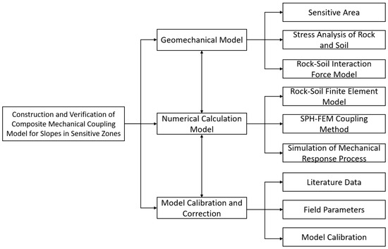
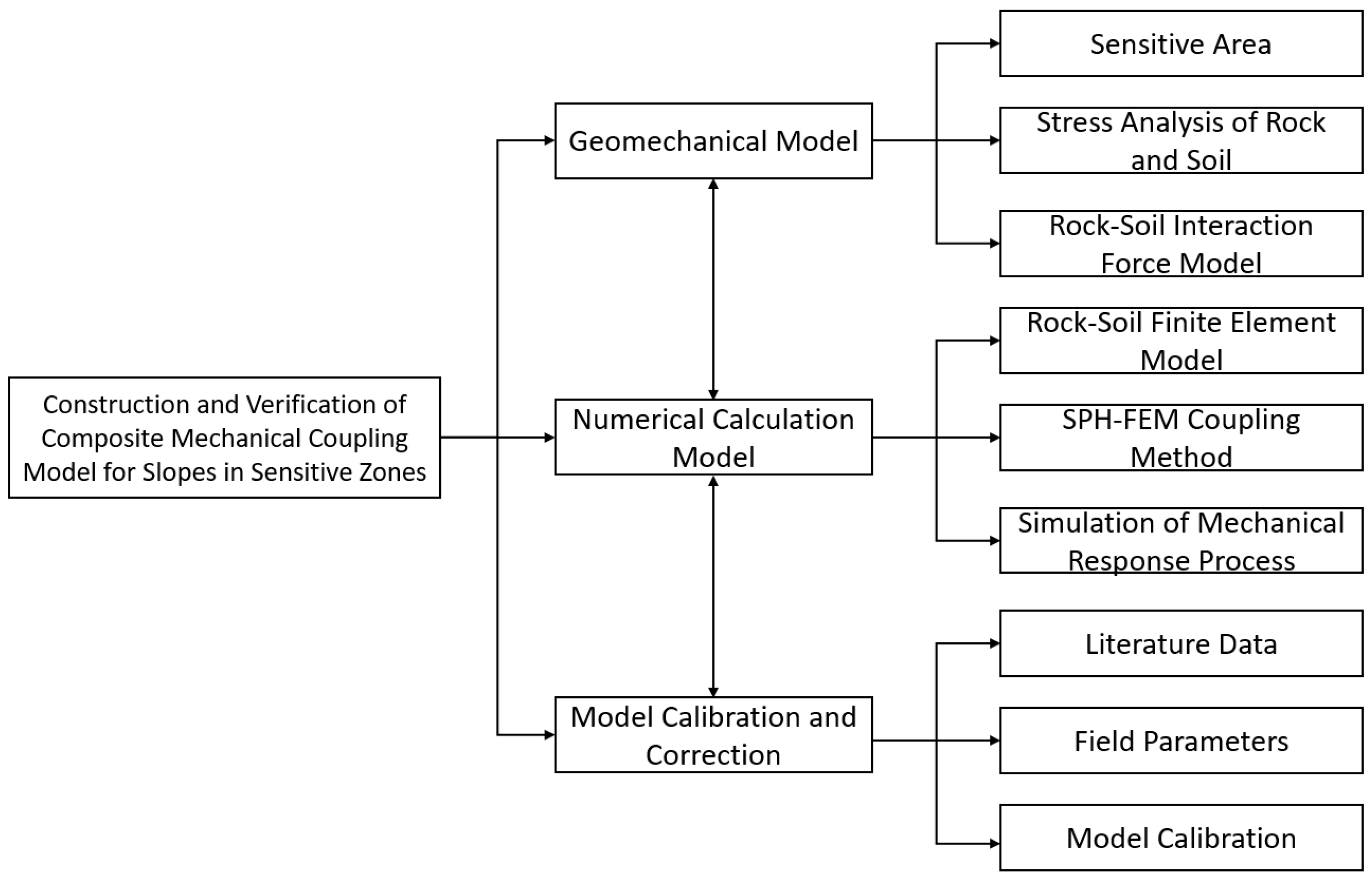
Based on the established mechanical analysis and calculation model for the composite pipe, verify the accuracy and reliability of the model, and complete the correction and optimization of model parameters and algorithms, as shown in Figure 1.

Figure 1. Model construction and verification approach.

2.2.1. Analysis of Pipe–Soil Interaction Process

Considering factors such as the coupling and deformation between the composite pipe and the soil, a numerical model for buried pipelines in sensitive areas is established. Taking the typical section of the Tieshanpo No. 1 gas gathering branch pipeline as the research object, the pipe–soil interaction is characterized using a contact surface model, in which the pipeline is designated as the master surface and the soil as the slave surface. The relevant parameters are listed in Table 1.

Table 1. Relevant factor parameters.

Transportation Conditions	Transportation Pressure	7~9 MPa
Transportation conditions	Transportation temperature	33~39 °C
Environmental conditions	Soil temperature	8~24 °C
Pipe specifications	Pipe diameter	323.9 mm
	Pipe wall thickness	12 + 3/15 + 3 mm
	Pipe length	70 m
Pipe laying	Pipe burial depth	1.2~4.2 m
Soil function of pipes	Contact surface friction coefficient	0.3
Area division	Sensitive area length	30 m
Pipe material	Base pipe material	L360QS
	L360QS Ultimate Strength	620 MPa
	L360QS Yield Strength	520 MPa
	Inner liner pipe material	UNSN08825
	UNSN08825 Ultimate Strength	620 MPa
	UNSN08825 Yield Strength	310 MPa

2.2.2. Pipeline Mechanical Analysis

Based on the Winkler assumption, the soil resistance conforms to a bilinear model. In this context, the Winkler assumption idealizes the soil–pipe interaction by representing the soil as a series of independent linear springs, i.e., the soil reaction force per unit length is proportional to the local pipe deflection. The bilinear model defines the soil resistance as linearly increasing with displacement in the elastic stage, followed by a plastic stage with a reduced stiffness or constant resistance after a specified yield displacement [28].

$$EI{\displaystyle \frac{d^4{y}^{\prime }}{d{x}^{\prime 4}}}=q(x^{\prime })-p(x^{\prime })$$

(8)

Mechanical analysis is conducted separately for the inner and outer pipes within the sensitive area:

Mechanical Analysis of the Outer Pipe in the Sensitive Area: The deflection and rotation angle at the pipe interface are determined from the soil thrust.

$$y_0=y^{\prime }{|}_{x^{\prime }-0}={\displaystyle \frac{2Q_0\beta }{K}}+{\displaystyle \frac{M_0}{2EI{\beta }^2}}$$

(9)

Here, $y^{\prime }$ is the deflection of the outer pipe, and $x^{\prime }$ is the axial coordinate along the outer pipe, with the origin located at the pipe entrance to the sensitive area. $Q_0$ and $M_0$ represent the shear force and bending moment at this entrance ($x^{\prime }$ = 0), respectively, both determined from the soil thrust. The parameter $\beta$ is defined as $\beta =\sqrt[4]{K/\left(4EI\right)}$, where K is the modulus of subgrade reaction of the soil, E is the Young’s modulus of the outer pipe material, and I is the moment of inertia of the outer pipe cross-section.

Mechanical Analysis of the Inner Pipe in the Sensitive Area: According to deformation compatibility conditions, the rotation angles inside and outside the landslide body are equal. The pipeline deflection is obtained through symmetric boundary conditions.

$$y(x)={\displaystyle \frac{1}{EI}}\left\{\begin{array}{c}-{\displaystyle \frac{1}{2}}{M}_0{x}^2+{\displaystyle \frac{1}{18}}L{P}_0{x}^3-{\displaystyle \frac{P_0}{30L}}{x}^5\\ {\displaystyle \frac{P_0}{90L^2}}{x}^6+\left({\displaystyle \frac{1}{2}}{M}_{0}L-{\displaystyle \frac{1}{30}}{P}_0{L}^3\right)x\end{array}\right.+{\displaystyle \frac{2L{P}_0\beta }{3K}}+{\displaystyle \frac{M_0}{2EI{\beta }^2}}$$

(10)

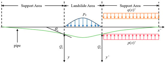
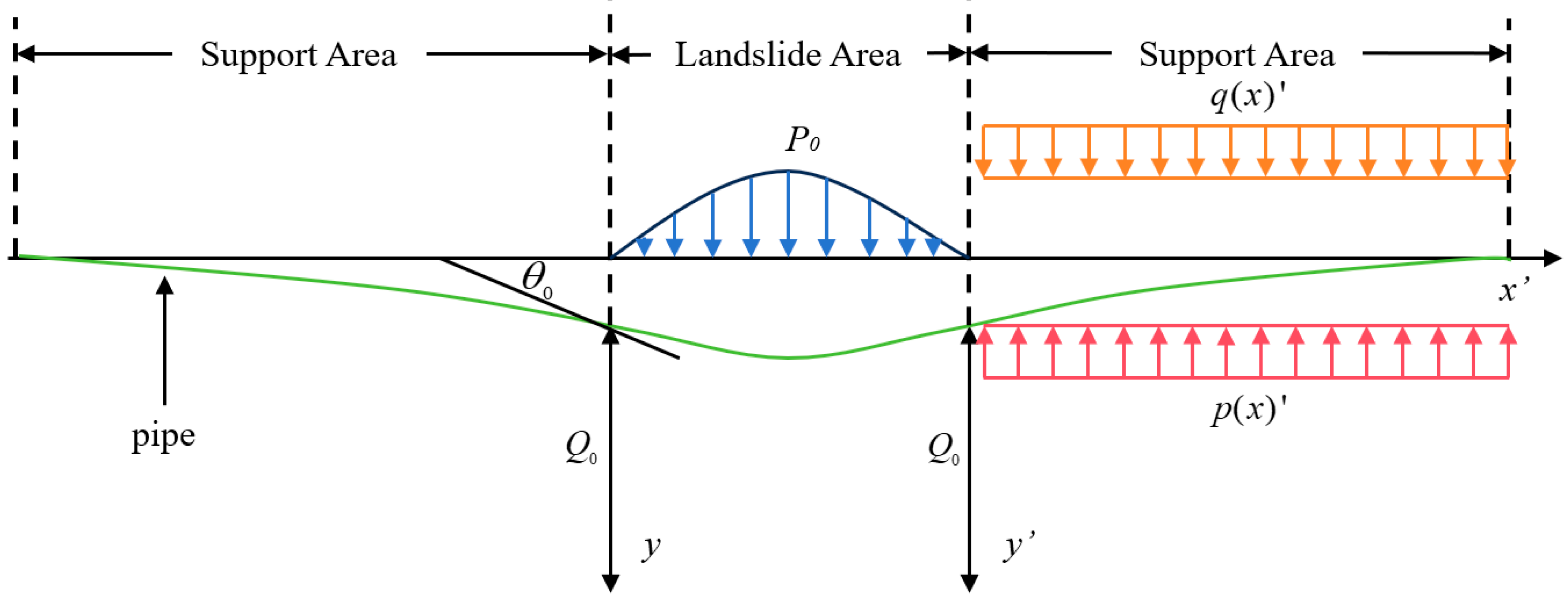
In this equation, $y(x)$ is the deflection of the inner pipe at axial coordinate $x$, where the origin is set at the center of the landslide area (as illustrated in Figure 2). The parameter $L$ denotes the half-length of the landslide-affected zone, i.e., the distance from the center to either boundary of the landslide area. The total length of the pipeline segment considered in the analysis is therefore 2$L$. The boundaries at $x=\pm L$ correspond to the interfaces between the landslide area and the support areas in Figure 2, where the soil is assumed to be stable; accordingly, both deflection and slope are set to zero at these boundaries. $P_0$ is the equivalent lateral soil pressure acting on the outer pipe within the sensitive area.

Figure 2. Mechanical analysis of pipelines under landslide action.

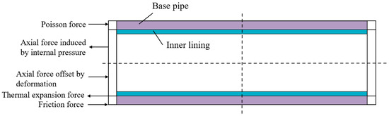
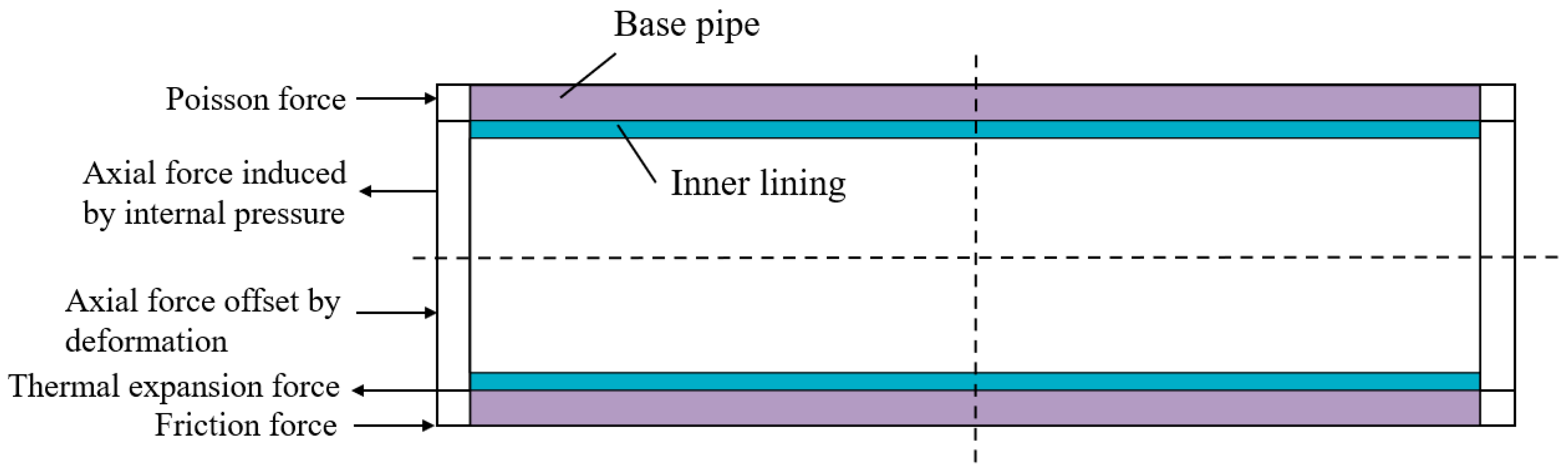
Simultaneously, the pipeline force analysis involves the action of various forces. A specific force schematic diagram is shown in Figure 3 (including the base pipe and liner pipe structures, as well as Poisson force, axial force induced by internal pressure, axial force offset by deformation, thermal expansion force, friction force, etc., covering the anchored section and virtual anchored section).

Figure 3. Mechanical Analysis of Bimetallic Composite Pipes.

2.2.3. Numerical Calculation Model Construction

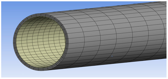
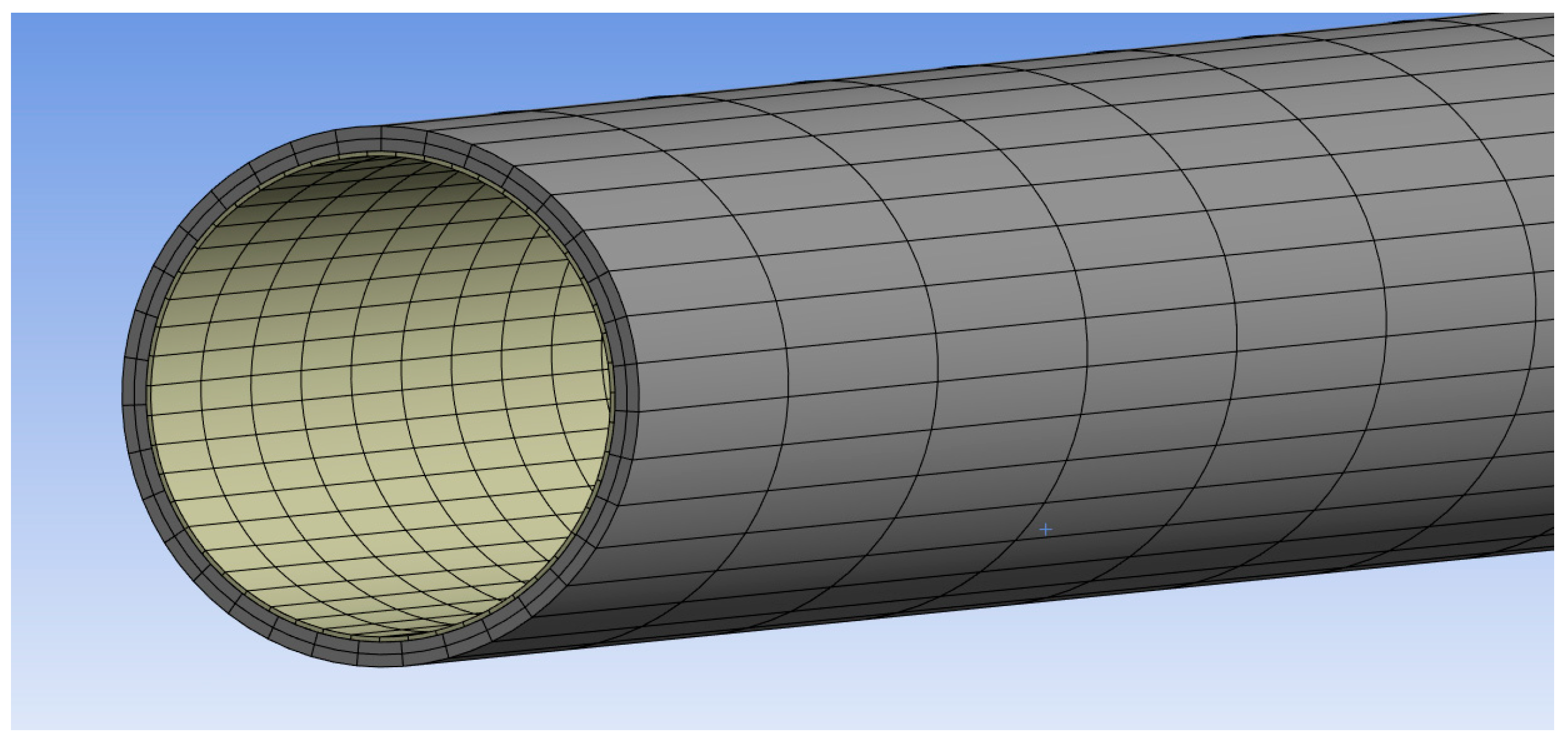
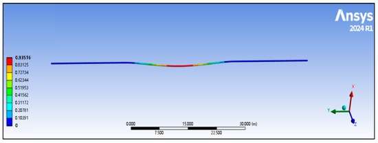
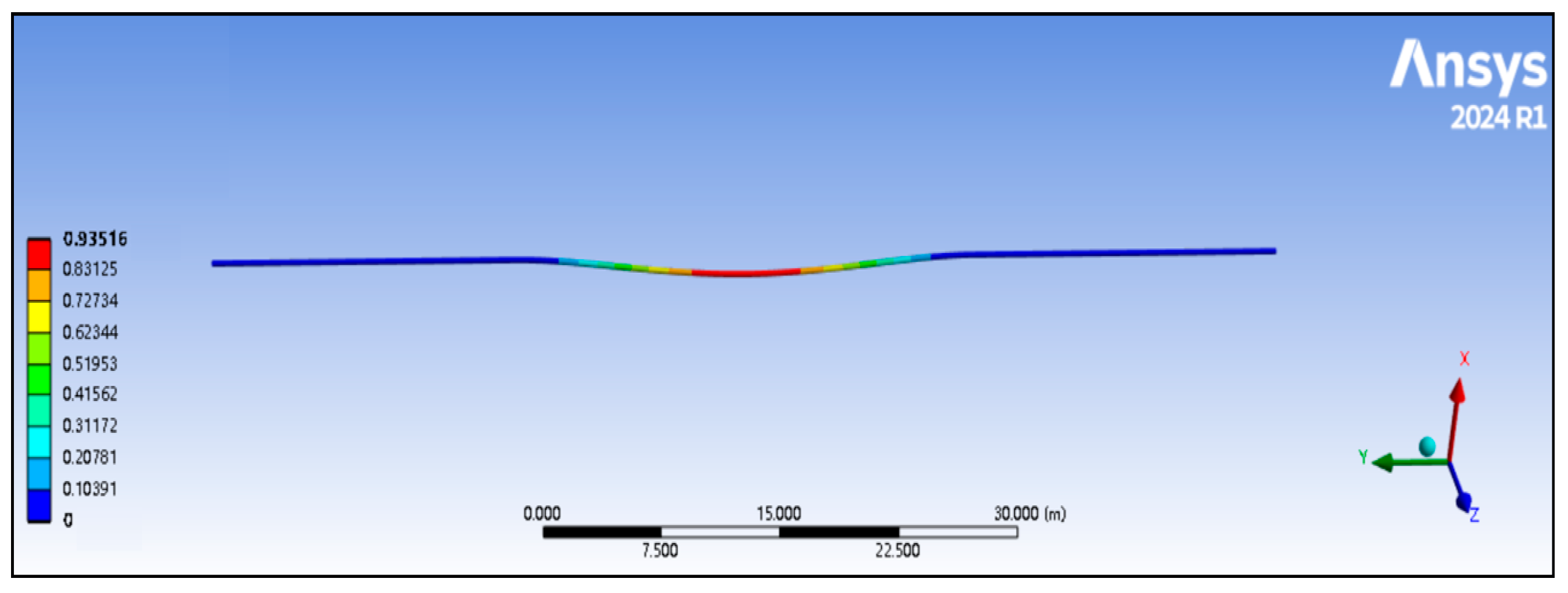
A numerical calculation model was developed using the professional finite element analysis (FEA) software ANSYS Mechanical 2024 R1, which is developed and distributed by ANSYS Inc., Canonsburg, PA, USA. The mesh division of the model is shown in the figure; SOLID186 solid elements are used. To improve computational efficiency, the mesh is refined in the key areas near the pipeline and the soil, while a coarser mesh is used for soil regions far from the pipeline to balance computational accuracy and resource consumption. Boundary conditions: for the soil, the bottom surface is fully fixed, lateral surfaces have symmetric constraint, and the top surface is free; the left and right ends of the soil are also fully fixed. For the pipeline, both ends are fixed supports with all six degrees of freedom constrained. To accurately simulate the mechanical response process of the composite pipe in sensitive areas under specific operating conditions, the simulation time was set to 1 s. Calculations from this model yielded the total deformation of the pipeline: the maximum deformation reached 0.93516 m, and the minimum deformation was 0 m. A detailed analysis was further conducted on the distribution of deformation along the pipeline length. Using the pipeline axial position as the horizontal axis and deformation as the vertical axis, the specific distribution data is as follows: at an axial position of 0 m, the deformation was 0.000 m; at 7.500 m, the deformation increased to 0.10391 m; at 15.000 m, the deformation was 0.20781 m; at 22.500 m, the deformation reached 0.31172 m; and at the axial position of 30.000 m, the deformation peaked at 0.93516 m. Intermediate deformation values of 0.41562 m, 0.51953 m, 0.62344 m, 0.72734 m, and 0.83125 m were also observed. This clearly demonstrates the pattern of gradually increasing deformation along the pipeline length, intuitively reflecting the deformation characteristics of the pipeline under the simulated conditions. The total deformation diagrams for the grid division and simulation are shown in Figure 4 and Figure 5 respectively.

Figure 4. Model grid division.

Figure 5. Software-generated deformation cloud map of the pipeline.

The physical and structural parameters for the pipeline in the model are set as follows:

Physical Parameters: Density is 7850 kg/m³; Isotropic Secant Coefficient for thermal expansion is 1.2 × 10⁻⁵ per °C.

Structural Parameters: Isotropic Elasticity (derived from Young’s modulus and Poisson’s ratio); Young’s modulus is 2 × 10¹¹ Pa; Poisson’s ratio is 0.3; Bulk modulus is 1.667 × 10¹¹ Pa; Shear modulus is 7.6923 × 10¹⁰ Pa.

2.2.4. Numerical Calculation Model Calibration and Verification

➀

Calibration Condition Settings: Two pipe specifications were selected: 323.9 × (12 + 3) mm and 323.9 × (15 + 3) mm. Operating pressure was set at 9 MPa; operating temperature at 38 °C; and ambient temperature at 23.5 °C.

Calibration Method and Results: Model calibration was performed by comparing the simulation results with the experimental and numerical data reported in Xu et al. [29], where a similar buried pipeline crossing a transverse landslide was analyzed using a three-dimensional finite element model with nonlinear contact and the same strain-based failure criterion The element types, pipe–soil contact conditions, mesh division, and boundary settings adopted in our model were validated against the reference model, showing consistent mechanical response trends.

➁

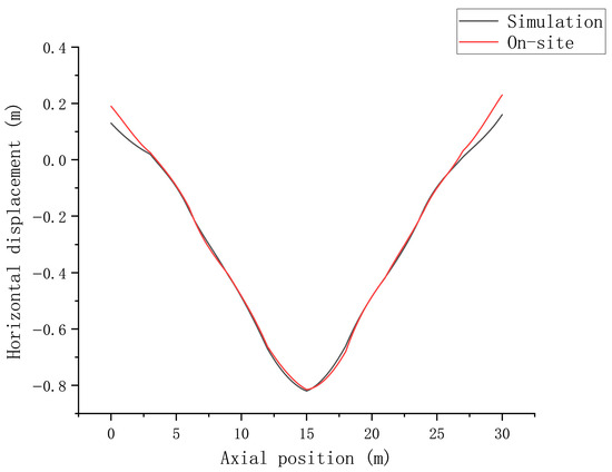
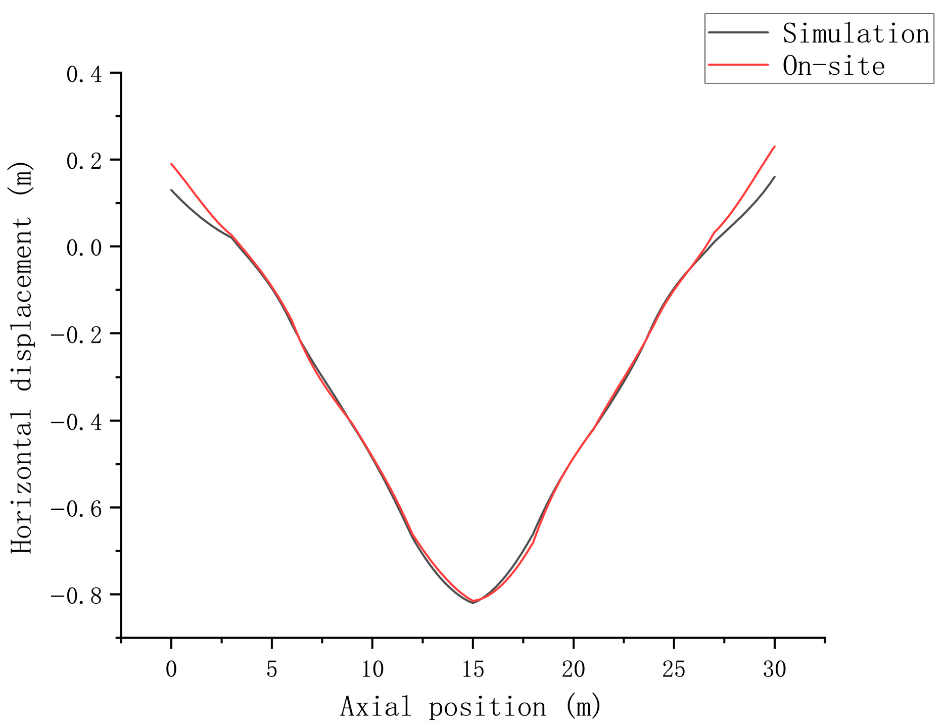
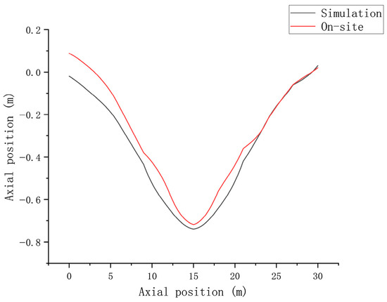
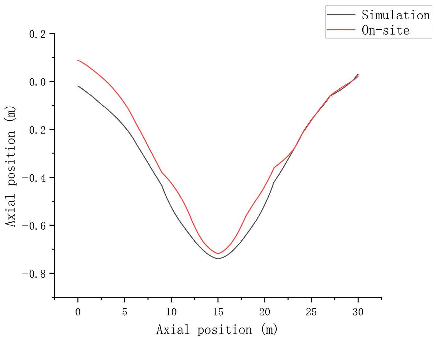
Simulation vs. Experiment Comparison: A comparison between field tests and numerical simulations yielded a relationship curve between pipeline axial position (m) and corresponding deformation (m), within an axial position range of 0–35 m. The deformation values were in good agreement, demonstrating strong consistency between the two results. This further verifies the accuracy and reliability of the model. As shown in Figure 6 and Figure 7.

Figure 6. Horizontal displacement comparison.

Figure 7. Vertical displacement comparison.

3. Study on the Mechanical Response State and Stress Transfer Mechanism of Composite Pipes in Sensitive Areas

Based on orthogonal experimental design theory, numerical simulation schemes were formulated. Numerical experiments on the dynamic response of pipelines under the interaction of multiple factors—such as installation methods, internal pipeline pressure, soil properties, and burial depth—were conducted for sensitive areas in high-steep mountainous regions. This systematically analyzed the influence of each factor on the mechanical behavior of bimetallic composite pipes and their interaction patterns. Combined with ANSYS Mechanica 2024 R1 finite element simulation results, the characteristics of pipeline mechanical response in sensitive areas were investigated, with a focus on analyzing the distribution patterns of pipeline stress, strain, and displacement under geohazard actions. This preliminarily reveals the stress transfer mechanism in bimetallic composite pipes.

➀

Research Approach

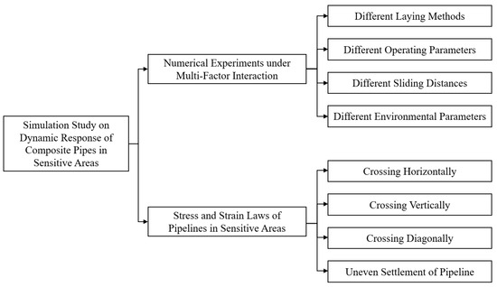
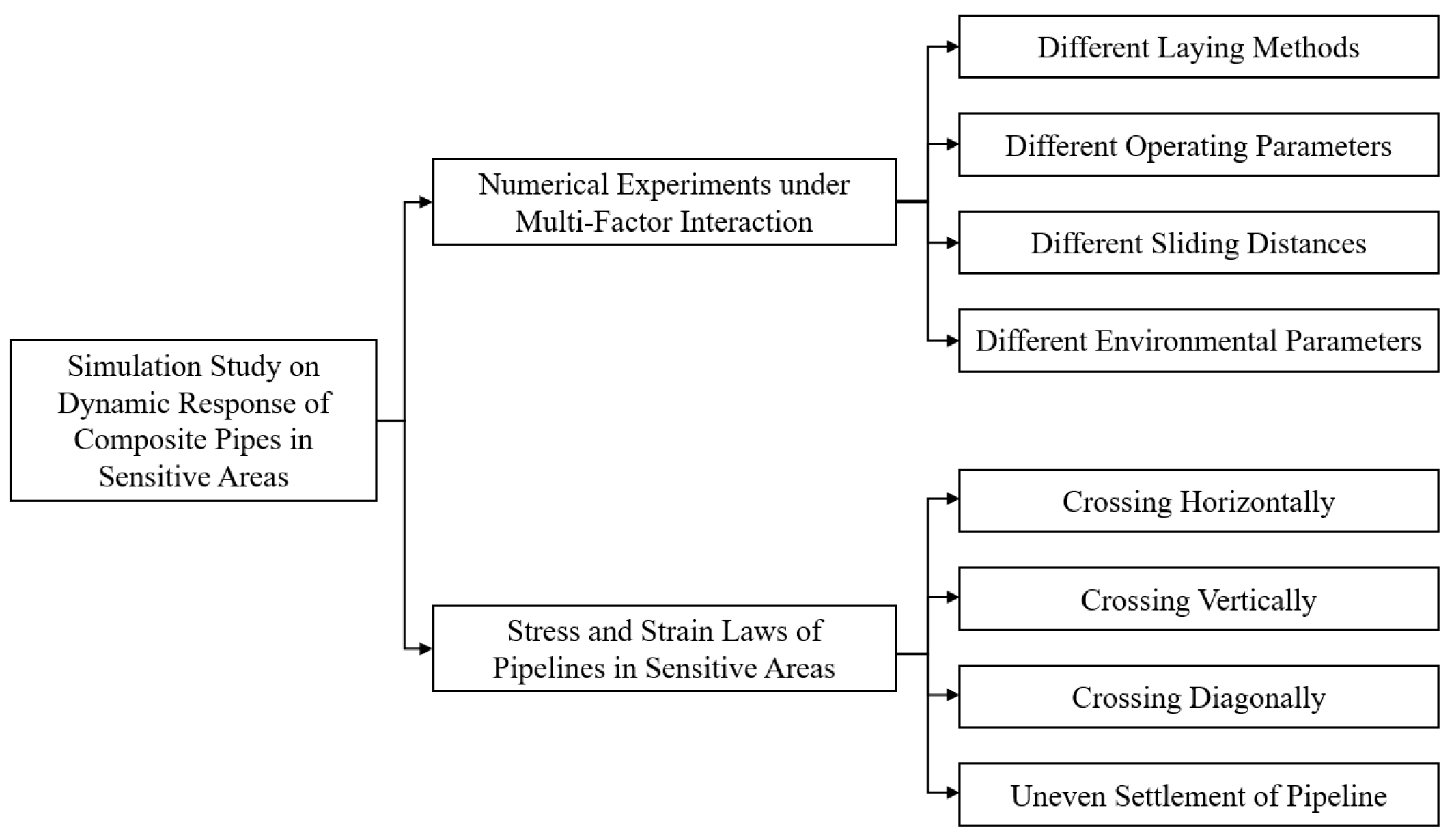
This section unfolds from two aspects: First, based on the previously constructed and validated finite element model of the composite pipe–soil coupling in sensitive areas, the orthogonal experimental design method was adopted. Key variables such as pipeline internal pressure, soil displacement in the sensitive area, and pipeline dimensions were set to conduct numerical simulation experiments under multi-factor interactions. Second, by extracting data on the hoop stress, axial stress, and Tresca stress of the composite pipe liner (UNS N08825) and base pipe (L360QS) from the simulation results, the influence patterns of each variable on pipeline mechanical behavior were analyzed. Combined with the characteristics of pipe–soil interaction, this reveals the stress transfer mechanism of bimetallic composite pipes, providing theoretical support for subsequent pipeline safety operation strategy formulation. The research approach is shown in Figure 8.

Figure 8. Research Ideas on the Mechanical Response State and Stress Transmission Mechanism of Composite Pipes in Sensitive Areas.

➁

Analysis of Mechanical Response of Composite Pipes under Multi-Factor Effects

(1)

Influence of Internal Pipeline Pressure on Mechanical Behavior of Composite Pipes

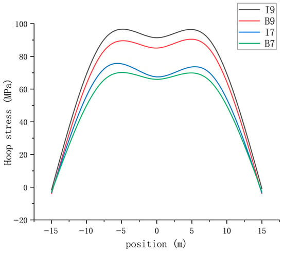
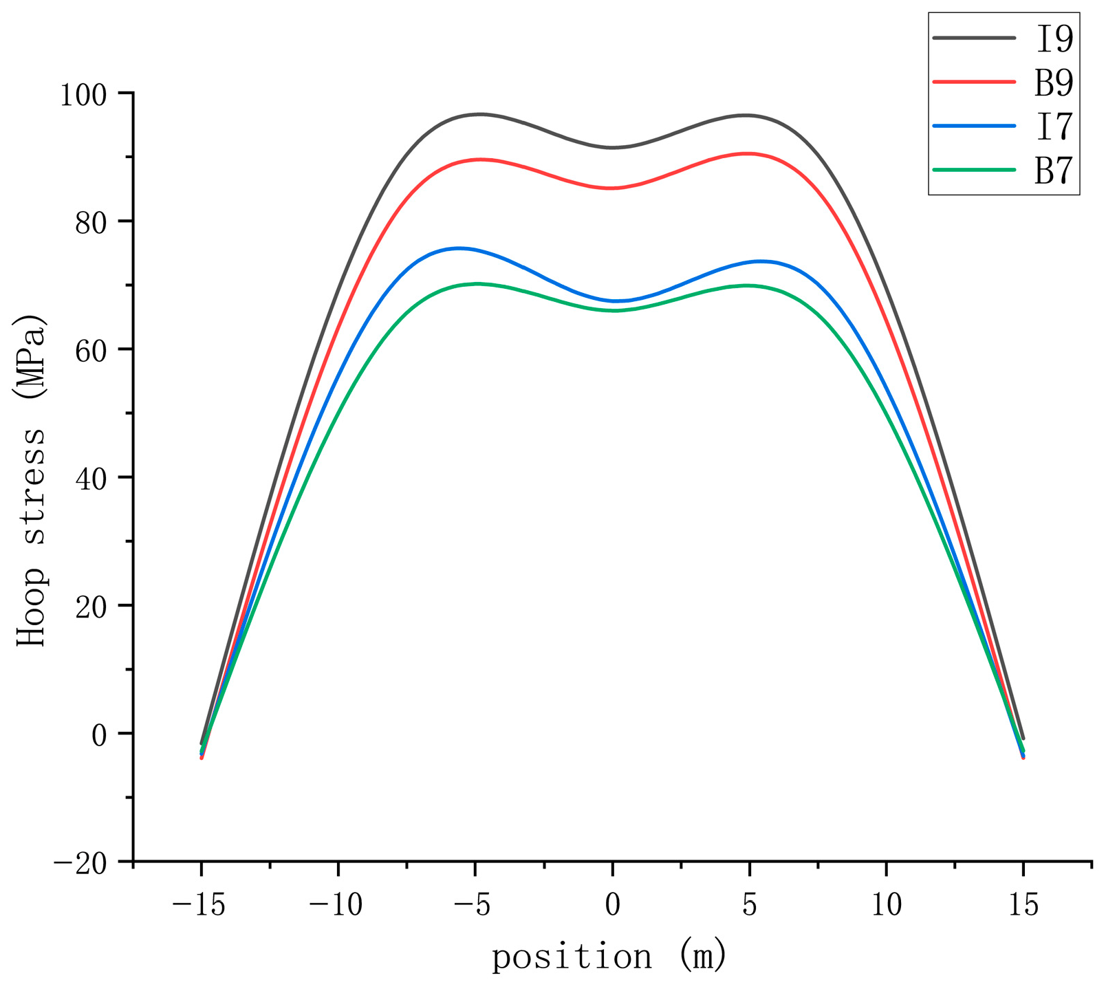
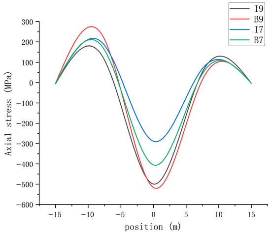
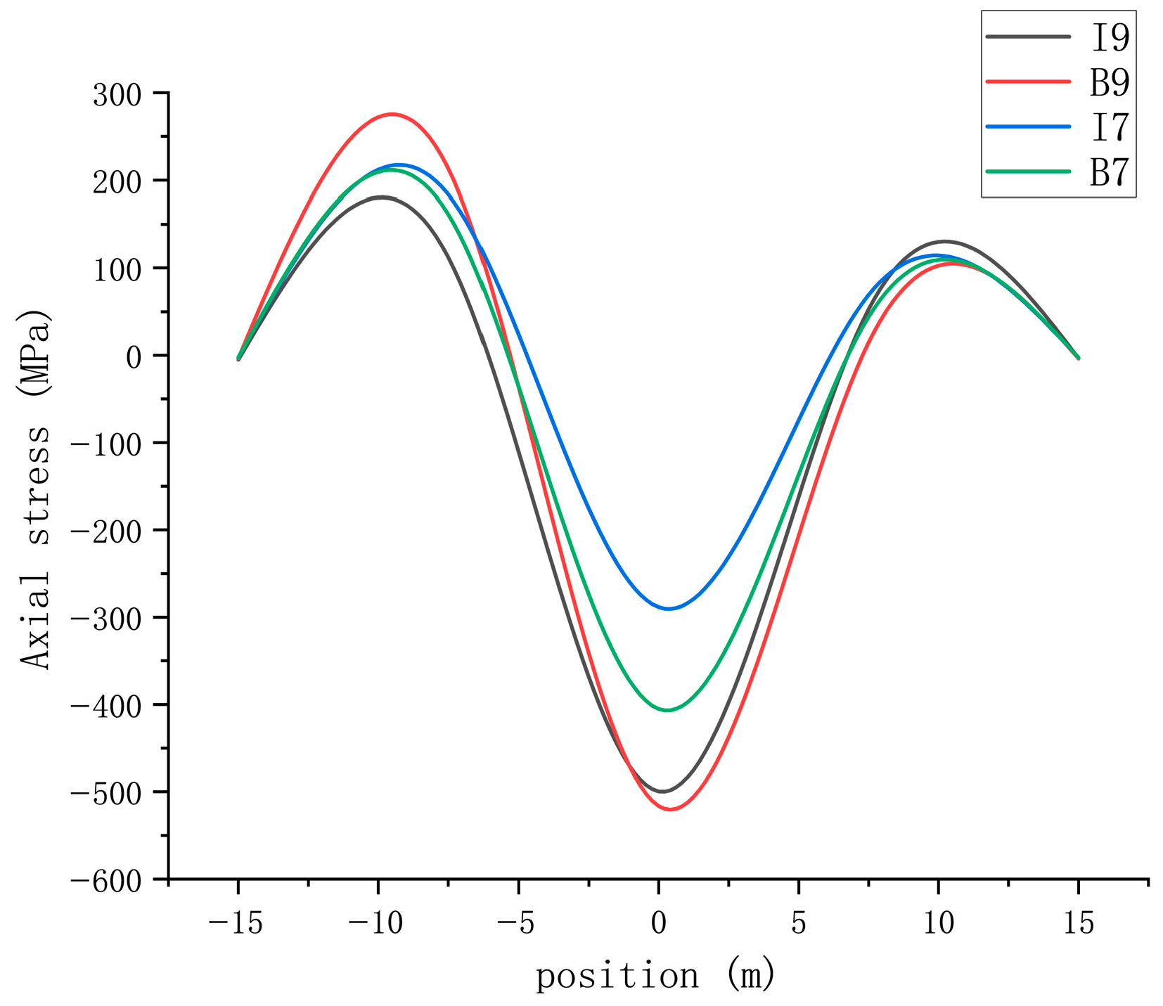
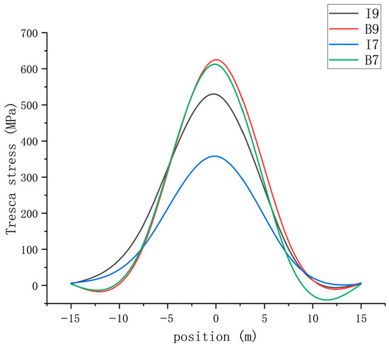
Taking a typical pipe section of the Tieshanpo No. 1 Gas Gathering Branch Line as the study object, the pipeline dimensions were selected as 323.9 × (base pipe 12 + liner 3) mm, the sensitive area length as 30 m, the soil friction coefficient as 0.3, and the ambient temperature as 23.5 °C. Two operating conditions with internal pressures of 7 MPa and 9 MPa were set to analyze the stress distribution characteristics of the composite pipe liner and base pipe when the soil displacement in the sensitive area is 1 m. The results are shown from Figure 9, Figure 10 and Figure 11.

Figure 9. Variation in hoop stress with internal pressure in the composite pipe.

Figure 10. Variation in axial stress with internal pressure in the composite pipe.

Figure 11. Variation in Tresca stress with internal pressure in the composite pipe.

In the figure, I9 represents the stress conditions of the liner pipe at 9 MPa, B9 represents the stress conditions of the base pipe at 9 MPa, I7 represents the stress conditions of the liner pipe at 7 MPa, and B7 represents the stress conditions of the base pipe at 7 MPa, respectively. As can be seen from the above diagram:

A. Pipeline stress exhibits a distribution characteristic of “high in the middle, low at both ends”. Stress is maximum at the center of the sensitive area (0 m) and approaches zero at both ends (±15 m), conforming to the mechanical transfer law of pipe–soil interaction under landslide action.

B. Internal pressure has a significant impact on pipeline stress: When internal pressure increased from 7 MPa to 9 MPa, the hoop stress of the liner pipe at the center of the sensitive area increased from 67.46 MPa to 91.41 MPa, an increase of 35.5%; the axial stress of the base pipe increased from −405.16 MPa to −516.48 MPa, an increase of 27.5%; the Tresca stress of the liner pipe increased from 357.97 MPa to 529.38 MPa, an increase of 48.0%.

C. A stress transfer effect exists: under the same internal pressure, the axial stress and Tresca stress show certain differences between the liner and the base pipe. For example, at an internal pressure of 9 MPa, the axial stress at the center of the liner is −499.75 MPa, while that of the base pipe is −516.48 MPa; the Tresca stress of the liner is 529.38 MPa, while that of the base pipe is 625.02 MPa. This indicates that under internal pressure, stress is transferred through the mechanical bonding interface between the liner and the base pipe, with the base pipe bearing more axial load.

(2)

Influence of Sensitive Area Displacement on Mechanical Behavior of Composite Pipes

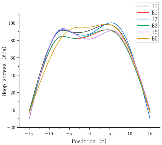
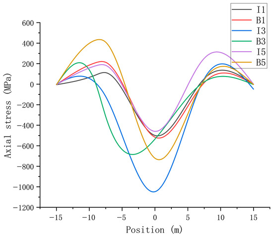
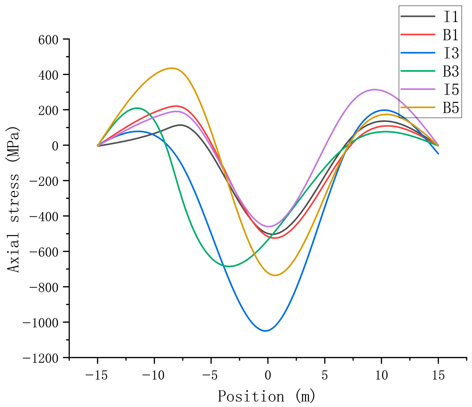
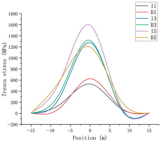
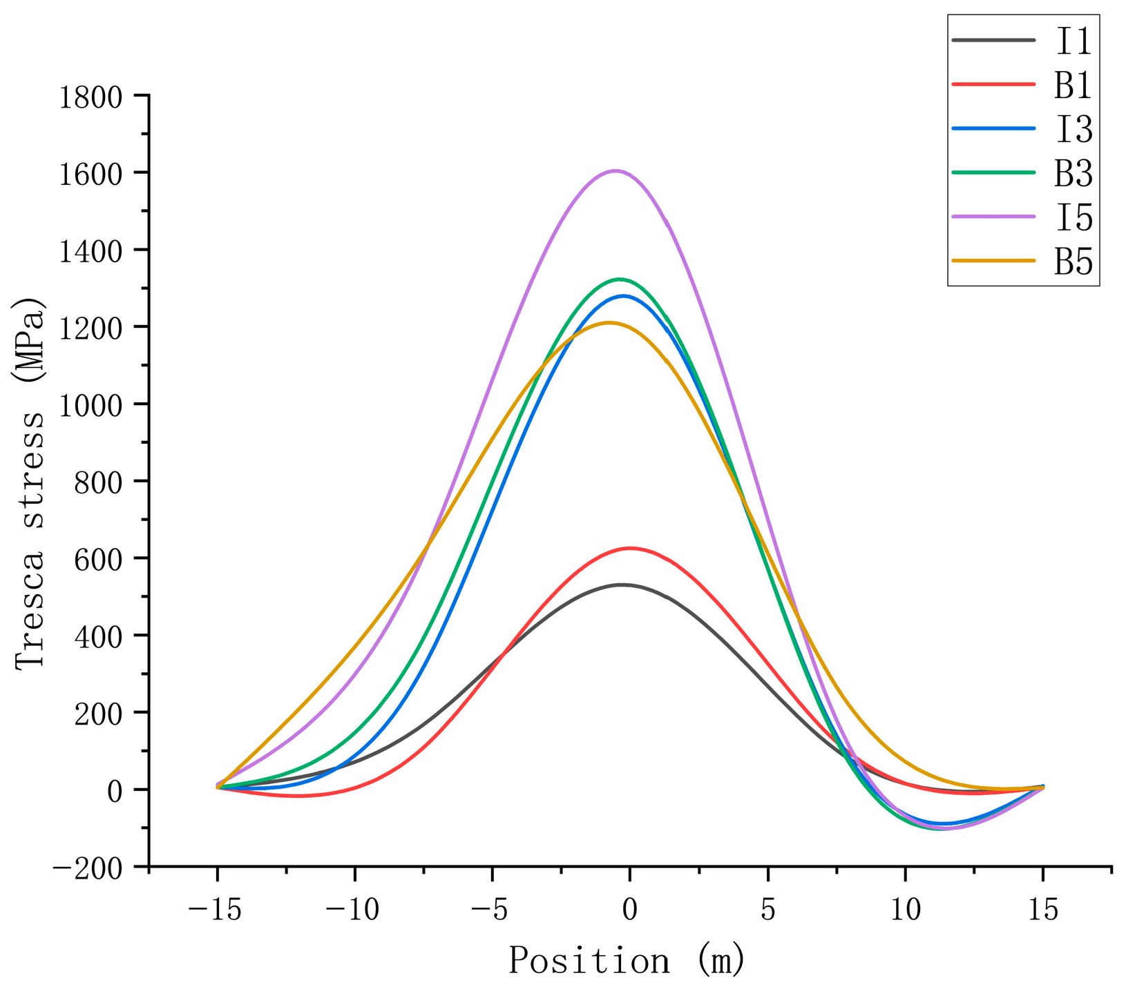
Keeping pipeline dimensions (323.9 × (12 + 3) mm), internal pressure (9 MPa), and ambient temperature (23.5 °C) constant, three operating conditions with sensitive area soil displacements of 1 m, 3 m, and 5 m were set to simulate the effect of landslide sliding distance on composite pipe stress. Results are shown from Figure 12, Figure 13 and Figure 14.

Figure 12. Analysis of Circumferential Stress in Composite Pipes under Displacement in Different Sensitive Areas.

Figure 13. Analysis of Axial Stress in Composite Pipes under Displacement in Different Sensitive Areas.

Figure 14. Analysis of Tresca Stress in Composite Pipes under Displacement in Different Sensitive Areas.

In the figure, I1 represents the stress conditions of the liner pipe when the soil displacement in the sensitive area is 1 m, B1 represents the stress conditions of the base pipe when the soil displacement in the sensitive area is 1 m, I3 represents the stress conditions of the liner pipe when the soil displacement in the sensitive area is von, B3 represents the stress conditions of the base pipe when the soil displacement in the sensitive area is 3 m, I5 represents the stress conditions of the liner pipe when the soil displacement in the sensitive area is 5 m, and B5 represents the stress conditions of the base pipe when the soil displacement in the sensitive area is 5 m, respectively. As can be seen from the above diagram:

A. As the sensitive area displacement increases, the stress in the liner and base pipe shows a reverse trend of “liner decreasing, base pipe increasing”: When displacement increased from 1 m to 5 m, the center axial stress of the liner changed from −499.75 MPa to −459.81 MPa, a decrease of 8.0%, while the center axial stress of the base pipe increased from −516.48 MPa to −721.92 MPa, an increase of 39.7%; the Tresca stress of the liner increased from 529.38 MPa to 1593.1 MPa, an increase of 200.8%, and that of the base pipe increased from 625.02 MPa to 1197.5 MPa, an increase of 91.6%.

B. Displacement has a more significant impact on base pipe stress: At 3 m displacement, the increase in the base pipe’s center axial stress compared to the 1 m condition was only 3.6%, but at 5 m displacement, the increase reached 39.7%. To quantitatively define this critical threshold, the von Mises yield criterion was applied. At a displacement of 3 m, the maximum von Mises stress in the base pipe reached 518.6 MPa, approaching the material’s yield strength of 520 MP. At displacements below 3 m, the base pipe remained elastic, whereas at 5 m, the equivalent stress exceeded the yield strength by 15.3%, indicating significant plastic deformation. Therefore, 3 m is identified as the critical displacement marking the transition from elastic to plastic behavior, beyond which the base pipe bears the main anti-sliding load and is prone to plastic deformation.

C. Stress fluctuation characteristics at both ends: As displacement increases, the hoop stress of the liner at both ends of the sensitive area decreases from −1.59 MPa to −10.54 MPa, then slightly recovers to 0.038 MPa. This reflects the change in pipe–soil interface frictional resistance, which first strengthens and then weakens with increasing displacement, consistent with the mechanical properties of soil transitioning from elastic deformation to plastic flow.

The negative hoop stress arises from three mechanisms:

(i)

Poisson effect due to axial constraint: Both ends of the pipeline are fully fixed. Internal pressure tends to elongate the pipe axially, but this elongation is prevented by the fixed supports, inducing axial compressive stress. Through Poisson’s ratio (ν = 0.3), axial compression leads to circumferential contraction, i.e., negative hoop stress.

(ii)

Bending–pressure coupling at the boundary: At x = ±15 m, the pipeline transitions from the displaced landslide zone to the stable soil zone. A significant bending moment gradient exists at this location, and the bending stress component can superimpose with the pressure-induced hoop stress, locally producing compression on certain fibers of the liner cross-section.

(iii)

Liner-base pipe interface slip: The liner is much thinner than the base pipe. At the highly constrained boundary, the base pipe preferentially resists soil reaction, while the liner may undergo slight inward radial deformation or local micro-wrinkling, further contributing to a compressive hoop stress state.

When the landslide displacement increases to 5 m, the bending effect becomes dominant and even overcomes the compressive trend, resulting in a slightly positive hoop stress (0.038 MPa). Therefore, the negative hoop stress observed in Figure 12 is not an error in sign convention or simulation, but rather a physically meaningful indication that the liner at the sensitive-area boundary is in a complex, multi-axial stress state dominated by axial constraint and bending, rather than by pure internal pressure.

(3)

Influence of Different Pipeline Dimensions on Mechanical Behavior of Composite Pipes

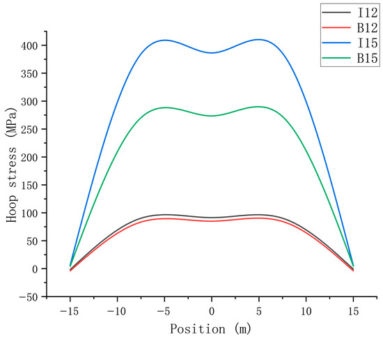
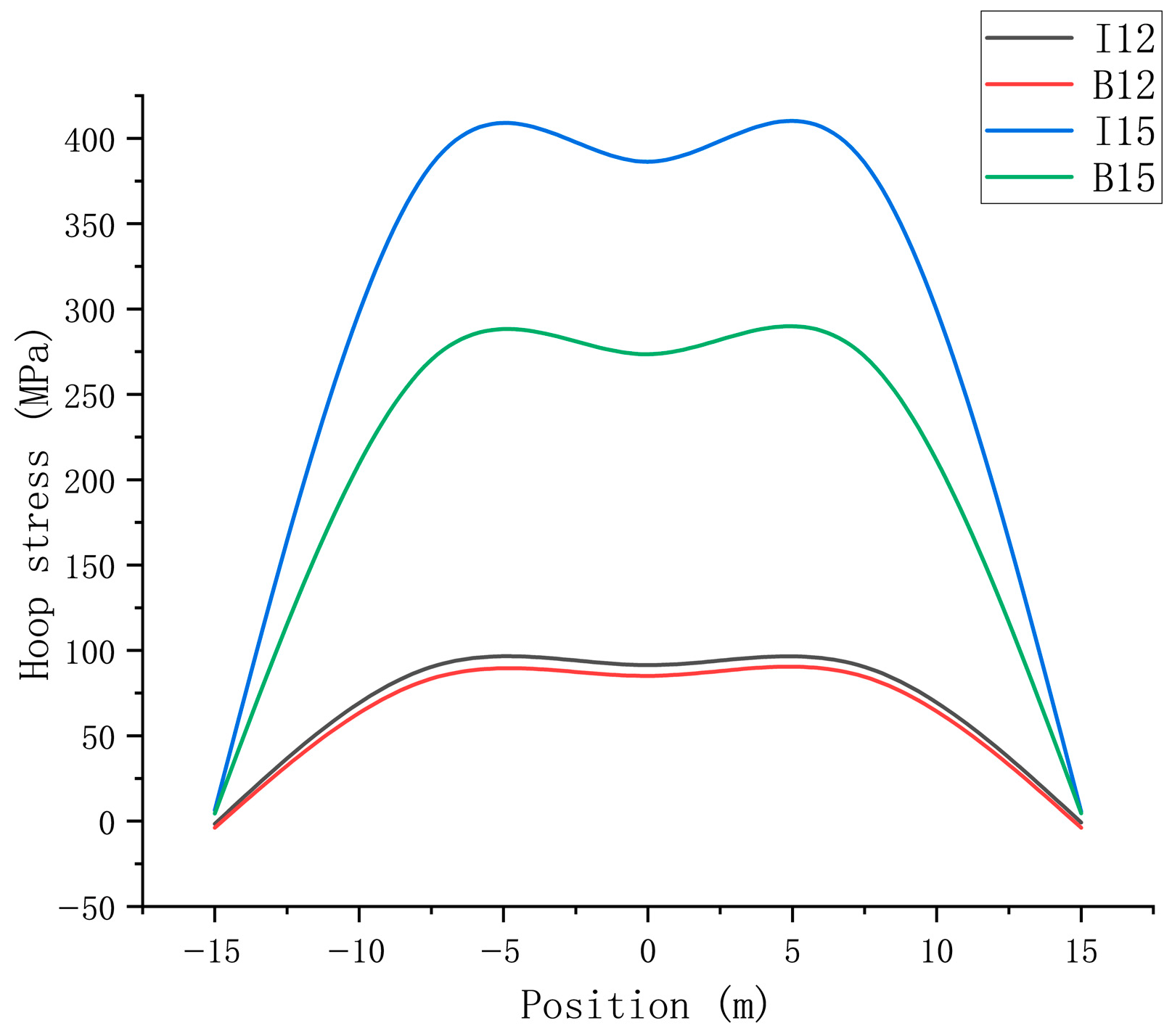
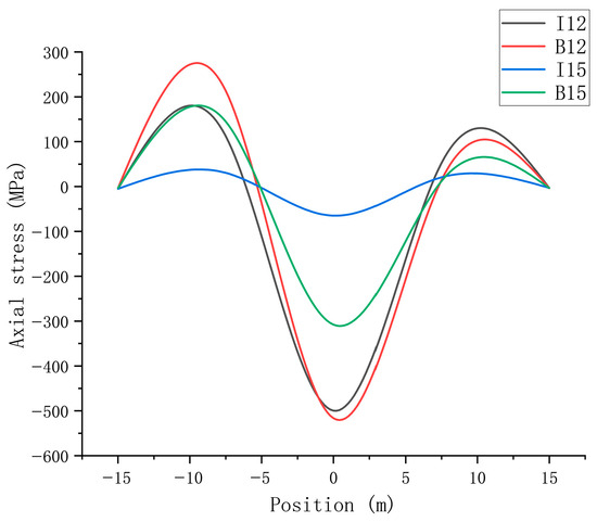
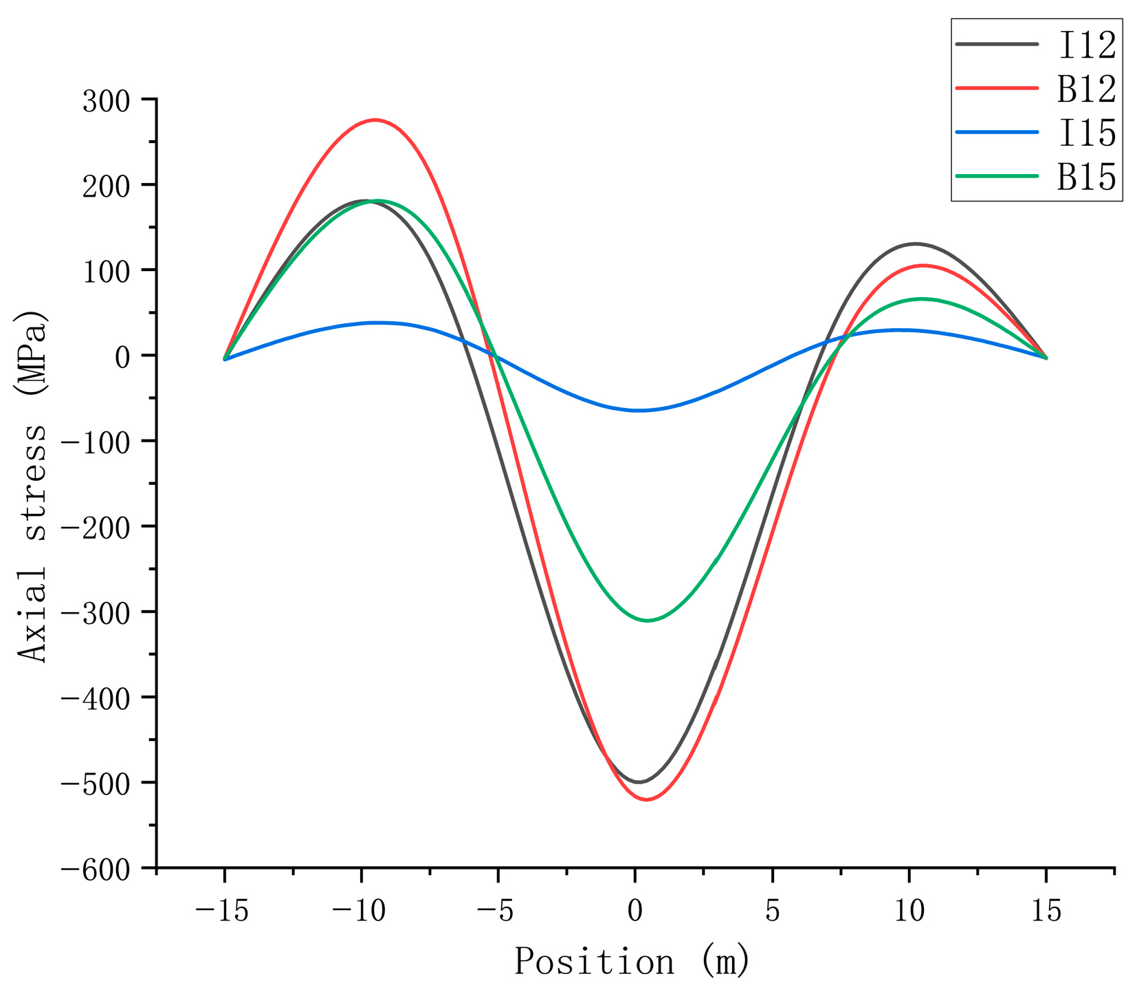
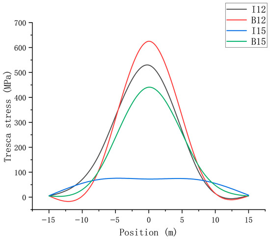
Two pipeline specifications were set: 323.9 × (12 + 3) mm (base pipe 12 mm) and 323.9 × (15 + 3) mm (base pipe 15 mm). Keeping internal pressure at 9 MPa, sensitive area displacement at 1 m, and ambient temperature at 23.5 °C, the influence of base pipe wall thickness on composite pipe stress was analyzed. Results are shown from Figure 15, Figure 16 and Figure 17.

Figure 15. Analysis of Circumferential Stress in Composite Pipes under Different Pipe Sizes.

Figure 16. Analysis of Axial Stress in Composite Pipes under Different Pipe Sizes.

Figure 17. Analysis of Tresca Stress in Composite Pipes under Different Pipe Sizes.

In the figure, I12 represents the stress conditions of the liner pipe when the base pipe size is 12 cm, B12 represents the stress conditions of the base pipe when the base pipe size is 12 cm, I15 represents the stress conditions of the liner pipe when the base pipe size is 15 cm, and B15 represents the stress conditions of the base pipe when the base pipe size is 15 cm, respectively. As can be seen from the above diagram:

A. Increasing base pipe wall thickness can significantly reduce pipeline stress: When the base pipe thickness increased from 12 mm to 15 mm, the center axial stress of the base pipe decreased from −516.48 MPa to −307.8 MPa, a reduction of 40.4%, and the Tresca stress of the base pipe decreased from 625.02 MPa to 440.88 MPa, a reduction of 32.7%. The center axial stress of the liner decreased from −499.75 MPa to −65.01 MPa, a reduction of 86.9%, indicating a weakened stress transfer effect. This disproportionate reduction is explained by the cubic relationship between bending stiffness and wall thickness (EI ∝ t³); a modest increase in base pipe thickness significantly reduces its deformation, thereby limiting load transfer to the liner.

B. Differences in hoop stress distribution: For the thin-walled base pipe section, the center hoop stress of the liner is higher than that of the base pipe, whereas for the thick-walled base pipe section, the center hoop stress of the liner is significantly higher than that of the base pipe. This indicates that a thick-walled base pipe can share more hoop load through its own stiffness, reducing stress concentration in the liner.

C. Stress transfer efficiency: The stress difference between the liner and base pipe narrows for the thick-walled base pipe. For example, the Tresca stress difference changed from 95.64 MPa to a negative value of −338.14 MPa. This suggests that increasing the base pipe wall thickness can optimize the stress transfer path, reducing the risk of liner buckling instability due to excessive stress.

➂

Summary

Through multi-factor numerical simulation experiments and stress analysis, the mechanical response characteristics and stress transfer mechanism of bimetallic composite pipes in the Tieshanpo sensitive area are preliminarily revealed:

(1)

Internal pipeline pressure, sensitive area displacement, and base pipe wall thickness are key factors affecting pipeline mechanical behavior. Among them, sensitive area displacement has the most significant impact on base pipe stress, while increasing base pipe wall thickness is the most effective in reducing overall stress.

(2)

The stress transfer mechanism manifests as: Under internal pressure, stress is transferred bidirectionally through the mechanical bonding interface between the liner and base pipe, with the base pipe bearing the main axial load. Under landslide displacement, stress transfers from the soil to the base pipe, and then to the liner via friction, exhibiting a progressive transfer characteristic of “soil → base pipe → liner”.

(3)

The center and both ends of the sensitive area are key locations for stress concentration, requiring focused attention in subsequent safety operation strategies. Risks can be mitigated through measures such as optimizing installation methods (e.g., longitudinal installation to reduce transverse landslide impact), adjusting operating internal pressure, and increasing base pipe wall thickness.

(4)

Discussion on the Near-Zero Hoop Stress at the Boundaries of the Sensitive Area

As shown in Figure 9, the hoop stress at both ends of the sensitive area (x = ±15 m) approaches 0 MPa, even though the pipeline is pressurized at 9 MPa. It is important to clarify that these “ends” refer to the boundaries of the landslide-affected zone, not the physical ends of the entire 70 m pipeline. At these boundaries, the soil transitions from the sliding zone to the stable zone, and the pipeline displacement is forced to nearly zero by the surrounding stable soil, as evidenced by the total deformation contour in Figure 5.

Under such confinement, the radial expansion of the pipe—which is the primary source of hoop stress under internal pressure—is severely restricted. Consequently, the hoop stress contributed by internal pressure diminishes locally, and the stress state at the boundary is dominated by soil reaction and bending moments rather than by pressure-induced tension. This phenomenon is consistent with Saint-Venant’s principle, which states that the influence of boundary constraints is limited to a local region. Therefore, the near-zero hoop stress at x = ±15 m does not contradict pressure vessel theory; instead, it reflects the fact that these locations are governed by boundary effects rather than by a pure internal-pressure condition.

4. Conclusions

This study investigates the mechanical transfer mechanism of bimetallic composite pipes in high-acid gas fields located in high-steep mountainous areas. Through material constitutive model optimization, pipe–soil coupling modeling, multi-factor response analysis, and combined experimental and field validation, the following core conclusions are drawn:

➀

The optimized material constitutive model can accurately characterize the mechanical properties of bimetallic composite pipes: For the stainless steel liner, the improved Ramberg–Osgood equation (Rasmussen model) was employed, showing a deviation of <5% from experimental data before the strength limit, thereby addressing the overestimation of strength in the high-stress stage by traditional equations. For the external base pipe pipeline steel, a segmented constitutive model accurately reflects its two-stage strain hardening characteristics of “initial yielding-transition-large yielding”, providing a reliable foundation for mechanical analysis.

➁

The constructed pipe–soil coupling finite element model for high-steep mountainous areas demonstrates significant reliability: Based on the geological and installation parameters of the Tieshanpo area, the simulation yielded a maximum pipeline deformation of 0.93516 m, with a deviation of <8% from the axial displacement measured in field tests. The model’s element types, mesh, and boundary conditions meet accuracy requirements.

➂

Internal pressure, sensitive area displacement, and base pipe wall thickness significantly influence the mechanical response of bimetallic composite pipes: When internal pressure increased from 7 MPa to 9 MPa, the hoop stress at the center of the liner increased by 35.5%, with the base pipe bearing the primary axial load. When displacement exceeded the critical value of 3 m, the stress increase in the base pipe surged sharply. Increasing the base pipe wall thickness from 12 mm to 15 mm reduced the center axial stress in the base pipe by 40.4% and in the liner by 86.9%, effectively optimizing stress transfer.

➃

The stress transfer in bimetallic composite pipes in high-steep mountainous areas exhibits a “dual-path progression”: Under internal pressure, it follows a bidirectional transfer along “liner → base pipe”. Under landslide displacement, it follows a unidirectional progression along “soil → base pipe → liner”. The center and both ends of the sensitive area are key locations for stress concentration. Optimization suggestions include longitudinal installation, base pipe wall thickness ≥ 15 mm, and internal pressure ≤ 7 MPa.

The findings of this research can provide theoretical support for the design and safe operation of bimetallic composite pipes in high-acid gas fields within high-steep mountainous areas. Future work could further introduce multi-field coupling effects to improve long-term performance prediction.

Despite these contributions, this study has certain limitations. The current analysis assumes steady-state internal pressure and quasi-static landslide displacement, whereas actual operating conditions often involve pressure fluctuations and dynamic loads. Future research will focus on the mechanical response of bimetallic composite pipes under cyclic pressure variations and dynamic geological loads, as well as the long-term performance of the liner-base pipe interface under such conditions.

References

- Zhang, G.J.; Dou, L.Z.; Xu, Y. Opportunities and challenges of natural gas development and utilization in China. Clean Technol. Environ. Policy 2019, 21, 1193–1211. [Google Scholar] [CrossRef] [Scilit]
- Zhao, W.; Jia, A.; Zhang, G. Analysis and countermeasures of natural gas development in China. Front. Eng. Manag. 2019, 6, 477–484. [Google Scholar] [CrossRef] [Scilit]
- Yang, Z.Z. Bimetal Composite Pipe for Oil and Gas Gathering and Transportation; Petroleum Industry Press: Beijing, China, 2018; pp. 1–25. [Google Scholar]
- Yang, Z.Z.; Wang, G.F.; Yan, K.; Wei, Y.Q.; Li, A.Q.; Du, Z.Q.; Lu, W.Z. Status and trend of girth welding procedure and joint strength design for bimetallic composite pipes. Oil Gas Storage Transp. 2017, 36, 241–248, 254. [Google Scholar]
- Li, F.G.; Wei, B.; Shao, X.D.; Cai, R. Double compound metal pipe used in high corrosion oil and gas fields. Oil Gas Storage Transp. 2010, 29, 359–362. [Google Scholar]
- Reda, A.; Kaspary, T.; Montague, P.; Shahin, M.; Meneze, E. Full-Scale Testing of Corrosion Resistant Alloy-Mechanically Lined Pipes for Submarine Pipelines. J. Offshore Mech. Arct. Eng. 2025, 147, 041501. [Google Scholar] [CrossRef] [Scilit]
- Zhou, S.J.; Guo, C.X.; Zhang, Y.F. Application of bimetal pipe in the offshore oil and gas engineering. China Pet. Chem. Stand. Qual. 2011, 31, 115–116. [Google Scholar]
- Hu, C.; He, Y.; Ma, K.; Wang, W.; Wang, L. Corrosion-Resistant Alloy Clad or Lined Steel Pipe for Submarine Pipeline. In Proceedings of the ISOPE International Ocean and Polar Engineering Conference, Ottawa, ON, Canada, 19–23 June 2023. ISOPE-I-23-443. [Google Scholar]
- Nie, H.L.; Ma, W.F.; Zhao, X.W.; Ma, Q.R.; Luo, J.H. Application status and analysis of bimetallic composite pipe in oil and gas pipelines. Heat Treat. Met. 2019, 44, 515–518. [Google Scholar]
- Wang, F.C.; Li, W.; Han, L.H. Interaction behavior between outer pipe and liner within offshore lined pipeline under axial compression. Ocean Eng. 2019, 175, 103–112. [Google Scholar] [CrossRef] [Scilit]
- Guo, Y.R.; Zhang, J.X.; Qin, Q.H.; Tan, D.S. Liner Buckling and Collapse of Bi-material Metal Pipes Subjected to Combined Loading. Chin. J. Solid Mech. 2019, 40, 342–353. [Google Scholar]
- Li, Y.; Li, J.Y.; Liu, Z.L. Real-time research on pipeline installation by reel-laying method based on finite element analysis. Ocean Eng. 2019, 37, 35–41, 150. [Google Scholar]
- Zhu, Z.X.; Yang, L.; Wang, F.C.; Fang, C. Combination effect and bearing capacity analysis of bimetallic composite pipes under axial compression. Ocean Eng. 2019, 37, 98–106. [Google Scholar]
- Liang, G.P.; Wang, B.; Wang, M.R.; Lan, X.C.; Wu, Z.; Du, W.F.; Wang, X.Y.; Wen, S.L. Failure analysis of girth weld of 316L-lined bimetallic composite pipe. Weld. Pipe Tube 2017, 40, 34–38. [Google Scholar]
- Gavriilidis, I.; Karamanos, S.A. Bending and buckling of internally-pressurized steel lined pipes. Ocean Eng. 2019, 171, 540–553. [Google Scholar] [CrossRef] [Scilit]
- Hilberink, A.; Gresnigt, A.M.; Sluys, L.J. Liner wrinkling of lined pipe under compression: A numerical and experimental investigation. In Proceedings of the International Conference on Offshore Mechanics and Arctic Engineering, Honolulu, HI, USA, 16–17 February 2010; Volume 49132, pp. 311–322. [Google Scholar]
- Yuan, L.; Kyriakides, S. Liner wrinkling and collapse of bi-material pipe under axial compression. Int. J. Solids Struct. 2015, 60, 48–59. [Google Scholar] [CrossRef] [Scilit]
- Hu, C.; Li, X.F.; Xiong, H.R.; Lang, Y.M. Corrosion resistance alloy pipe for subsea pipeline in offshore oil and gas field. Petrochem. Equip. 2015, 85–89. [Google Scholar]
- Li, G.; Jiang, Y.; Zhang, P.F.; Meng, X.W. Application of Reel-Lay in installation of subsea mechanically lined pipe. China Pet. Mach. 2018, 48, 48–51. [Google Scholar]
- Chaudhuri, C.H.; Choudhury, D. Buried pipeline subjected to seismic landslide: A simplified analytical solution. Soil Dyn. Earthq. Eng. 2020, 134, 106171. [Google Scholar] [CrossRef] [Scilit]
- Tsatsis, A.; Gelagoti, F.; Gazetas, G. Performance of a buried pipeline along the dip of a slope experiencing accidental sliding. Géotechnique 2018, 68, 968–988. [Google Scholar] [CrossRef] [Scilit]
- Wang, J.; Li, C.D.; Liang, D.M.; Liu, Q. Mechanical analysis and control strategy of pipeline beneath landslide area under different crossing angles. In Proceedings of the International Conference on Pipelines and Trenchless Technology, Xi’an, China, 18–20 October 2013. [Google Scholar]
- Zeng, D.Z.; Yang, B.; Sun, Y.X.; Zhu, D.J.; Shi, T.H.; Lin, Y.H. Finite element simulation and experimental study on hydro-forming of lined steel pipe. Dri. Prod. Technol. 2010, 33, 78–79. [Google Scholar]
- Macdonald, M.; Rhodes, J.; Taylor, G.T. Mechanical properties of stainless steel lipped channels. In Proceedings of the 15th International Specialty Conference on Cold-Formed Steel Structures, St. Louis, MI, USA, 19–20 October 2000. [Google Scholar]
- Olsson, A. Stainless Steel Plasticity: Material Modelling and Structural Applications. Ph.D. Thesis, Luleå Tekniska Universitet, Luleå, Sweden, 2001. [Google Scholar]
- Rasmussen, K.J.R. Full-range stress–strain curves for stainless steel alloys. J. Constr. Steel Res. 2003, 59, 47–61. [Google Scholar] [CrossRef] [Scilit]
- Hertelé, S.; De Waele, W.; Denys, R. A generic stress–strain model for metallic materials with two-stage strain hardening behaviour. Int. J. Non-Linear Mech. 2011, 46, 519–531. [Google Scholar] [CrossRef] [Scilit]
- Hetényi, M. Beams on Elastic Foundation; University of Michigan Press: Ann Arbor, MI, USA, 1946. [Google Scholar]
- Xu, G.L.; Chen, L.P.; Jiang, X.C.; Cai, L.X. Study on strain response characteristics of buried pipelines laterally crossing landslide section. J. Saf. Sci. Technol. 2023, 19, 149–155. [Google Scholar]
Disclaimer/Publisher’s Note: The statements, opinions and data contained in all publications are solely those of the individual author(s) and contributor(s) and not of MDPI and/or the editor(s). MDPI and/or the editor(s) disclaim responsibility for any injury to people or property resulting from any ideas, methods, instructions or products referred to in the content. |
© 2026 by the authors. Licensee MDPI, Basel, Switzerland. This article is an open access article distributed under the terms and conditions of the Creative Commons Attribution (CC BY) license.