


Abstract
Shaped charge is widely used in petroleum drilling, yet the inherent parametric uncertainty of oil shale introduces significant uncertainties that affect perforation outcomes. The complex coupling of oil shale constitutive parameters under extreme strains poses challenges for uncertainty quantification. A coupled algorithm integrating an improved material point method (MPM) and polynomial chaos expansion (PCE) is presented, and polynomial chaos expansion (PCE) is used to systematically analyze the uncertainty and sensitivity of shaped charge jet penetration depth. Mechanical parameters from oil shale samples at Checun Coal Mine well No. 1 were tested to define key parameter ranges and establish a reliable uncertainty space. A benchmark simulation of a single isolated shaped charge jet validated the algorithm, and Sobol’ global sensitivity analysis identified internal friction angle, density, and Poisson’s ratio as strongly sensitive parameters, while tensile strength, Young’s modulus, and cohesion showed weak sensitivity, supporting surrogate model dimensionality reduction. Composite detonation models of three and five charges further revealed the effects of multi-projectile blast wave coupling on jet dynamics, providing new theoretical insights into cluster effects under high-energy, high-pressure, and extreme-strain conditions. Sensitivity and uncertainty analyses based on surrogate models emphasized the critical influence of internal friction angle alongside Poisson’s ratio and density. A reliable numerical framework is established for multi-physics coupled simulations of geomechanical responses under complex multi-source explosive loading.
1. Introduction
Directional perforation is a critical engineering issue in the extraction of shale oil [1,2,3]. After casing the oil and gas well, perforating guns are used to fire perforating charges that penetrate the metal casing and cement sheath, establishing communication between the wellbore and the reservoir. This allows the fluidized minerals stored in the formation to be successfully extracted into the wellbore, thereby enabling normal production operations [4,5,6].
Currently, a widely adopted method is to couple the Lagrangian Finite Element Method (FEM) with the Smoothed Particle Hydrodynamics (SPH) method [7,8,9,10,11]. Mingfei Li et al. [12,13,14,15] used the LS-DYNA software to establish a complete numerical model of the perforating gun, analyzing the variation in metal jet velocity over time and the number of perforating charges. They also examined the stress changes in the casing under impact load for different numbers of perforating charges. Ying-Song Lin [16,17] used LS-DYNA software, based on the FEM, to analyze the process of perforating charge penetration into oil shale, obtaining the damage mechanisms of oil shale during the penetration process. The results were compared with experimental data, and the distribution pattern of cracks near the perforation hole was summarized. Yan Yan et al. [18,19] established a physical model for the perforating charge penetration of concrete sheaths, obtaining experimental data on perforating charge penetration into the cement sheath. They also developed a numerical model using LS-DYNA software for analysis, comparing the results with experimental findings and confirming the damage mechanisms of the concrete sheath under jetting action. Bin Yu et al. [20] constructed numerical models of focused jet and high-pressure fracturing using LS-DYNA software, quantitatively analyzing the influence of perforating charge geometry and booster charge quantity on penetration performance. They conducted a surface experiment on compound blasting and directional seam creation in hard roof strata, clarifying the characteristics of crack propagation between adjacent perforation holes and verifying the rationality of the perforation parameters.
In the widely used Finite Element Method (FEM), during high-energy jetting and rapid compression deformation of the target material, issues such as mesh distortion and a significant reduction in time steps are commonly encountered [21]. This phenomenon not only severely affects computational efficiency but also significantly limits the simulation duration when using the Smoothed Particle Hydrodynamics (SPH) method to model focused jetting. The material point method (MPM), however, offers significant advantages in handling large deformation problems, as it does not require dealing with complex convective terms and effectively avoids mesh distortion issues commonly found in traditional mesh-based methods. The MPM uses a material point discretization model that carries all the material information, accurately reflecting the motion and deformation characteristics of the object. This advantage allows MPM to excel in simulating scenarios with extreme deformation, simplifying the computational process and greatly reducing the number of computational elements [22,23,24,25,26]. As a result, the time step remains stable in MPM when dealing with large deformation problems, without shrinking, enabling complete simulation of the physical process under fully simulated parameters.
Due to the combined influence of rock mass structure, surrounding environment, load conditions, geological age, and geological processes, the mechanical properties of rock masses often exhibit significant variations in different spatial locations and directions [27,28,29,30]. Calculating the parametric uncertainty of rock mass properties and quantifying their parametric uncertainty are critical for uncertainty analysis and optimizing perforation parameters to achieve optimized explosive penetration. For example, Tan Wenhui et al. [31] applied geostatistical theory to conduct field tests and statistical analyses of rock strength parameters and explored the variability of rock strength parameters. Although traditional sensitivity analysis or Monte Carlo methods can quantify uncertainty, their high computational costs and limitations in analyzing nonlinear response mechanisms in high-dimensional parameter spaces make them inefficient.
The polynomial chaos expansion (PCE) method is integrated into the framework. The impact of oil shale parameter uncertainties on the jet penetration depth is systematically analyzed. This coupled approach enables accurate predictions of the physical simulation results. This method can replace traditional simulation programs to achieve efficient prediction of simulation data. Based on this, the Sobol method [32,33,34] is used to solve the coefficients of the surrogate model, quantitatively analyzing the impact of various oil shale parameters on the performance of the focused jet. The material point method combines the advantages of the Lagrangian method and the mesh-free method, establishing connections between particles through a background grid, thereby avoiding the issue of time step reduction.
The MPM-PCE method provides a fast tool for uncertainty quantification. Past rock mechanics studies usually use machine learning and Bayesian inference [35]. Other reservoir models rely on static core-log data to quantify heterogeneity [36]. These traditional methods have clear limitations. Finite element grids break during high-strain explosive modeling. The material point method (MPM) uses a background grid to stop numerical crashing. The polynomial chaos expansion (PCE) builds a mathematical surrogate with very few MPM samples. This coupled approach directly solves the speed and stability problems of traditional uncertainty models.
2. The Motion Principle of Focused Jets
2.1. Principle of Shaped Charge
As shown in Figure 1, 2α is the shaped charge liner cone angle, β is the liner collapse angle relative to the axis, and γ is the angle between a liner element’s motion direction and surface normal. After collapse, the liner is driven by the detonation wave, converging toward point O at velocity v0 along the mother line. The liner metal rapidly melts and converges radially to the centerline; radial velocity cancels, converting kinetic energy into axial velocity, forming a jet head with velocity vj. The inner metal, obstructed by the outer jet, moves slower, collapsing axially as a tail slug with velocity vs.
Figure 1.
Schematic of jet velocity distribution.
The Gurney equation is a commonly used empirical formula in engineering for estimating the initial velocity of fragments. Based on this equation, the collapse of the shaped charge liner and the subsequent formation of a metal jet can be characterized by the consolidation velocity v0, the formation velocity vs, and the jet tip velocity vi, which can be expressed as follows:
where is the Gurney constant of the explosive; r is the charge-to-mass ratio of the configuration; α is the angle between the shaped charge liner surface and the central axis; β is the collapse angle, defined as the angle between the collapsing liner surface and the central axis; and γ is the angle between the direction of motion of the jet particles and the normal to the liner surface.
2.2. Engineering Principles
In engineering applications, upon initiation, the explosive undergoes detonation, generating a detonation wave and high-pressure gas. Under the confinement of the casing, these forces rapidly collapse the shaped charge liner inward toward the axis. The high temperature softens the liner and the internal metallic powder, which then collide along the central axis. This collision cancels the radial velocity component, resulting in a phase transition from solid to a high-velocity metal jet directed along the axis. The process of jet formation and its penetration into the target is illustrated in Figure 2.
Figure 2.
Directional slit formation of a concentrated energy jet.
The interaction of the jet with the oil shale upon contact can be divided into three stages:
- (1)
- Perforation Stage:
As shown in Figure 2a, copper-based metal powder within the shaped charge liner forms a high-velocity metal jet under the action of the detonation wave generated by the explosive combustion, moving rapidly along the axial direction. When the jet tip impacts the oil shale, it exerts an impact force on the contact surface far exceeding the oil shale’s yield strength, fracturing the oil shale and enabling penetration. During this stage, the jet exhibits its strongest penetration capability and highest velocity; however, due to the relatively small mass of the jet tip, the resulting borehole diameter is limited. This stage is extremely brief; once the jet’s kinetic energy is depleted, most of the material splatters and disperses, while a small portion continues moving within the borehole.
- (2)
- High-Velocity Penetration Stage:
As illustrated in Figure 2b, during this stage, the middle portion of the metal jet follows the jet tip, while the residual tip continues moving, driven by the jet momentum. Due to the relatively small kinetic energy loss and a larger mass compared to the jet tip, this stage results in a longer penetration channel with a borehole diameter larger than that of the perforation stage. The high-velocity penetration stage is critical for jet motion; since the penetration channel becomes deeper, the jet no longer loses material, and most of the jet mass remains within the channel.
- (3)
- Decelerated Penetration Stage:
As shown in Figure 2c, the slowest tail portion of the metal jet enters the borehole, marking the complete entry of the jet into the oil shale mass. At this stage, the mass of material within the borehole reaches its maximum. The tail portion further enlarges the diameter of the shallow borehole and pushes the jet tip and middle portions to continue advancing. As the penetration depth increases, the mass of the jet material gradually decreases, and the borehole diameter correspondingly reduces until the jet’s kinetic energy is fully dissipated, marking the end of the entire penetration process.
3. Principles of MPM-PCE Algorithm
3.1. Principles of MPM
The material point method (MPM), proposed by Sulsky, is a particle-based simulation technique grounded in continuum mechanics. MPM discretizes the continuum body into a set of Lagrangian material points, each carrying complete physical information, including material properties integrated through constitutive models (such as elastic modulus and tensile strength) and state variables incorporated via state equations (such as velocity and strain). The Eulerian background grid does not contain material physical information; it is used solely to compute and update momentum equations and spatial derivatives. Information transfer between the material points and the background grid is achieved through shape functions.
The simulation of large deformations is realized through the motion of the material points. Constitutive models update stresses, strains, and velocities on the material points in real time, thereby describing material motion, deformation, and failure modes. By combining the advantages of both Lagrangian and Eulerian frameworks, MPM avoids the need to handle convective terms explicitly and completely circumvents mesh distortion issues. This results in stable time stepping and makes MPM uniquely advantageous for simulating complex coupled composite materials, extremely large deformations, and severe failure experiments.
Figure 3 illustrates the computational procedure using a basic computational unit composed of four background grid nodes and twelve material points. The calculation process consists of four steps:
Figure 3.
Calculation procedure of MPM.
- (1)
- Particle Mapping to the Grid
As shown in Figure 3a, the first step involves calculating the grid node indices along with the corresponding shape functions and their gradients . At the same time, information carried by the particles, such as constitutive model variables and velocities, is mapped onto the background grid nodes:
where and are the mass and velocity of the particles, and and are the mass and velocity of the grid nodes.
- (2)
- Grid Node Update
As shown in Figure 3b, after the grid nodes receive material information mapped from the particles through the shape functions, the displacement and velocity of the grid are computed. Simultaneously, the grid undergoes corresponding displacements and deformations in coordination with these calculations.
where is the time step and t is the computation time.
- (3)
- Grid Mapping to the Particle
As shown in Figure 3c, the grid nodes are used to compute the displacement, velocity, stress, and strain of the particles. This information is then mapped back to the particles, which update their state variables accordingly and undergo displacement to update their positions.
where is volume of the particle and is body forces of the particle.
- (4)
- Grid Refresh
As shown in Figure 3d, the deformed background grid from Step 2 is reset to its initial configuration in preparation for the next computational step. This marks the completion of one full computation cycle.
3.2. Principle of Adaptive Particle Splitting
In the material point method (MPM) simulation process, interactions between particles are realized through the background grid. Therefore, particles located in different grid cells do not directly interact with each other. The computational model simulates the shaped charge jet. The detonation wave drives the jet formation. The liner undergoes intense stretching under this explosive action. The peak strains exceed 10. Under such conditions, numerical fracture is prone to occur, which can lead to distortion of the simulation results.
Severe strain causes numerical fracture. An adaptive particle splitting optimization algorithm is introduced. This algorithm solves the numerical fracture problem directly. Extreme deformation causes particle stretching beyond the continuum limit. This unphysical stretching creates artificial voids in standard MPM. Splitting prevents these voids and maintains material continuity. The splitting factor of 0.9 perfectly balances grid resolution and calculation speed. A higher factor leaves numerical voids. A lower factor explodes the total particle count. This specific factor ensures stable jet head simulations. At each time step, the cumulative strain of particles in the three principal directions is calculated.
First, the initial length of the particle is calculated as follows:
Then, the current characteristic lengths are calculated in the three directions:
When the characteristic length in any of the three principal directions exceeds , the particle will automatically split. After splitting, the spacing between particles becomes , as illustrated in Figure 4.
Figure 4.
Schematic diagram of the division of point. is the width of the background grid, and is the splitting factor.
After particle splitting, the newly created particles inherit the physical state variables such as stress and strain from the original particle, while extensive quantities such as mass, volume, and internal energy are divided equally between them.
After completing a computational step, the cumulative strain variables of the particles need to be adjusted accordingly. The equivalent length of the particle is halved in the splitting direction while remaining unchanged in the other directions. If the equivalent lengths of the particle change in all three directions after splitting, the cumulative strain carried by the particle must be adjusted accordingly. Based on the definition of L0, the initial length of the particle after splitting is given by
Assuming the particle splits along the xxx-direction, the equivalent length of the particle after splitting is
that is,
The strain adjustment formula relies on geometric compatibility. The physical deformation of the material remains constant during the particle splitting process. Equations (19) and (20) are substituted into the basic strain definition. This substitution yields the final adjustment formula for the cumulative strain:
3.3. Principle of Polynomial Chaos Expansion
Wiener introduced the homogeneous chaos method, this mathematical framework analyzes Gaussian stochastic processes [37]. This method is now known as polynomial chaos expansion (PCE). It enables accurate and efficient uncertainty quantification by constructing surrogate models that can predict physical processes and outcomes with high precision. The core principle involves expanding multiple variables using orthogonal polynomial bases, thereby transferring the randomness of the variables into the coefficients of the polynomials.
The model is initialized as . The variable in the model represents an -dimensional uncertain parameter, and Y is the model’s output dependent variable. Based on the Gaussian stochastic process, the polynomial chaos expansion is formulated using Hermite orthogonal polynomials as the basis functions:
where , , , , … are the coefficients to be determined and denotes the -th order Hermite orthogonal polynomial.
For the -dimensional -th-order Hermite orthogonal polynomial, , with the vector composed of different random variables in represented by ; it can be described as
By truncating Equation (30) and approximating it with a finite number of -th-order terms, assuming the total number of terms is mmm, Equation (30) can be simplified as
where is the expansion coefficients to be determined and is the Hermite orthogonal polynomials, which can be calculated using Equation (31); the above two form a complete set of orthogonal bases, satisfying the following condition:
where is the Kronecker delta function and is the inner product in Hilbert space; it can be defined as
where is the weight function corresponding to the orthogonal polynomial basis .
When corresponds to Hermite orthogonal polynomials, the weight function is the n-dimensional normal distribution function:
Subsequently, the known solution is projected onto the orthogonal polynomial basis to solve for the expansion coefficients , expressed as follows:
When Equation (24) is truncated at polynomial order and the dimensionality of the variables is , the number of terms mmm in the orthogonal polynomial expansion can be expressed as
The coefficients and number of terms in the polynomial chaos expansion can be determined using Equations (36) and (37). Leveraging the orthogonality of Hermite polynomials, the mean response of the original model to the random variables can be expressed as
where is the integration domain of dimension , According to Equation (38), the mean response corresponds to the coefficient of the zero-order term in the polynomial chaos expansion. By repeating the above procedure, the response variance can be ultimately obtained as
3.4. Procedure of MPM-PCE Algorithm
A non-intrusive algorithm was developed. This algorithm quantifies the influence of oil shale parameters. These parameters determine the final penetration depth of the shaped charge jets. The algorithm integrates Optimized Latin Hypercube Sampling (OLHS), polynomial chaos expansion (PCE), and Sobol global sensitivity analysis to perform a quantitative assessment of the impact of oil shale parameters. The computational procedure of the algorithm is as follows:
To comprehensively simulate the impact of parametric uncertainty of rock properties on the penetration depth of shaped charge jets, the algorithm employs the Optimized Latin Hypercube Sampling (OLHS) method [38]. OLHS ensures good uniformity of sampled parameters and is well suited for interval-based parameters. The number of sampling points is a critical factor affecting computational efficiency. First, the uncertain parameters that influence the penetration depth of the shaped charge jet into the rock are identified along with their probability distributions and value intervals. Then, by substituting the truncation order of the polynomial chaos expansion and the dimensionality of the uncertain parameters into Equation (22), the number of coefficients to be solved is determined. After establishing the number of coefficients, N sampling points are selected within the standard uncertainty space.
Subsequently, the sampled points are input into the MPM-based numerical simulation program to perform high-fidelity simulations of the physical process. The penetration depth obtained from these simulations serves as the foundational data for training the subsequent polynomial chaos expansion (PCE) model.
Using the sampled data points and the collected simulation results, a mathematical model is trained based on the polynomial chaos expansion (PCE) method to perform uncertainty quantification and enable accurate predictions of the simulation program. Replacing the high-fidelity simulation with this abstract mathematical model significantly improves computational efficiency, thereby making Sobol global sensitivity analysis feasible for highly complex physical processes.
Subsequently, to further validate the accuracy of the PCE surrogate model, an additional 20 sets of sampling points were generated within the constructed uncertainty space using the OLHS method. These samples were independently evaluated using both the PCE model and the MPM simulation program. The results from both approaches were then compared through fitting analysis to assess the predictive accuracy of the surrogate model.
Finally, based on the validated PCE surrogate model and the uncertainty space constructed using the OLHS method, a large number of sampling data were computed. The results were then incorporated into the Sobol global sensitivity analysis algorithm to quantitatively assess the influence of each oil shale parameter within its parametric uncertainty interval on the jet penetration depth. This analysis reveals the extent to which each parameter of oil shale affects penetration. After truncation, the polynomial chaos expansion (PCE) model can be decomposed using the Sobol method as follows:
where and is the subvector of X, which is obtained by extracting the components of V corresponding to the indices indicated by the subset.
Due to the uniqueness of the Sobol decomposition, the decomposition term can be expressed as
Owing to the orthogonality of the polynomial chaos basis, the variance of the polynomial expansion is given by
The Sobol sensitivity indices of the random parameters can thus be expressed in terms of the coefficients of the polynomial chaos model. Based on the polynomial chaos expansion, the first-order Sobol sensitivity index and the total sensitivity index can be determined via least-squares fitting, satisfying
expressed in matrix form as
where is the vector of the PC coefficients to be determined, is the observation vector of the model outputs, is the design matrix, the element , and is the residual vector.
When the sample size satisfies Equation (37), the coefficients are determined by solving the equation
At this point, the algorithm flow is complete. The algorithm integrates the Optimized Latin Hypercube Sampling (OLHS) method, polynomial chaos expansion (PCE), and Sobol sensitivity analysis and employs a non-intrusive approach to couple the main program with the MPM simulation. This enables automated analysis of the influence of parametric uncertainty in oil shale parameters on the penetration depth of shaped charge jets, significantly improving computational efficiency. The algorithm flow is illustrated in Figure 5.
Figure 5.
A computational flowchart of the MPM-PCE coupled algorithm.
4. Verification of Optimization Algorithm
During the motion of the shaped charge jet, the shaped charge liner and the internal metal powder undergo intense stretching under the powerful pressure of the detonation wave, with the jet experiencing maximum strains exceeding 10. However, in traditional MPM simulations, severe numerical fracture occurs at the jet head, resulting in distorted simulation outcomes, as shown in Figure 6.
Figure 6.
Diagram of numerical fracture.
Due to complete structural fracture and scattering of the jet head, the monitored particle velocity field exhibits a “marble effect”. The material points lose numerical stability because the shape functions fail, resulting in significant numerical oscillations and rendering the results meaningless for analysis. The numerical oscillations are shown in Figure 7, where the data display complete chaos, making any further analysis impossible.
Figure 7.
Diagram of numerical oscillation.
An adaptive particle splitting algorithm is introduced. This algorithm resolves the numerical fracture issue directly. The splitting factor α is a core parameter of the algorithm. If α is set too small, excessive particle splitting occurs, significantly increasing computational complexity. Conversely, if α is too large, the numerical fracture problem remains unresolved.
Therefore, to evaluate the effectiveness of the adaptive splitting algorithm and determine the optimized splitting factor, simulations were conducted with α values set to 1.0, 0.9, and 0.8. The velocity cloud maps of the jet head were collected and compared with the original case.
As shown in Figure 8, after introducing the adaptive splitting algorithm, the issue of numerical fracture was effectively mitigated. The jet head structure remained coherent and stable, enabling a more accurate simulation and reproduction of the jet formation process.
Figure 8.
Diagram of improved algorithm simulation.
A velocity–time comparison is shown in Figure 9. From the velocity contour plots, it can be seen that the adaptive particle splitting algorithm demonstrates strong applicability in handling extreme strain conditions. After enabling the algorithm, numerical oscillations are greatly mitigated. Moreover, due to the structural integrity, kinetic energy is better transmitted, resulting in an increased peak velocity at the jet head. The improved MPM thus provides a more accurate simulation of extreme strain engineering problems such as shaped charge jets.
Figure 9.
Comparison of jet head velocity with different splitting factors.
As shown in Figure 9, when the splitting factor α is set to 1.0, minor numerical oscillations still persist. However, setting α to 0.9 or 0.8 significantly improves numerical stability, with both cases exhibiting nearly identical stability. Notably, the numerical smoothness at α = 0.8 surpasses that at α = 0.9.
From the perspective of computational efficiency, when the splitting factor α is set to 0.9, the simulation time for the 0–0.4 ms period is 17 min, whereas setting α to 0.8 results in a simulation time of 91 min for the same period. Computational efficiency dictates the final parameter choice. The optimized splitting factor α is set to 0.9.
5. Numerical Model Validation
5.1. Strength Model and Equation of State
Accurate constitutive models are crucial for shaped charge jet simulations. The 5104 working face of Well No. 1 at Checun Coal Mine in Yan’an City is selected as the engineering background. This specific geological site provides the authentic constitutive characteristics of the oil shale. Samples were collected from the roof strata of the oil shale at the 5104 working face, followed by comprehensive mechanical parameter testing.
In accordance with the standards established by ISMR, samples of oil shale collected from the roof of the 5104 working face at Well No. 1, Checun Coal Mine, were prepared and tested. The constitutive parameters of the oil shale were comprehensively measured. The testing procedure is illustrated in Figure 10, and the test results are presented in Table 1.
Figure 10.
Experimental diagram of oil shale specimen.
Table 1.
Parameters of the oil shale specimen.
The Drucker–Prager (D-P) model provides necessary computational efficiency, whereas advanced models are required to capture high strain rates and pore collapse. In this study, the Riedel–Hiermaier–Thoma (RHT) constitutive model was tested against the D-P model in a comparative simulation. As illustrated in Figure 11, particle damage states are distinguished by color, red particles represent the damaged material regions, blue particles indicate the unaffected intact zones, the RHT model provides a more distinct characterization of the rock fragmentation process and produces superior visual damage morphology.
Figure 11.
Comparison of RHT model and Drucker–Prager (D-P) model.
Despite these visual differences, the discrepancy in final penetration depth between the two models is less than 0.8%. Given that the polynomial chaos expansion (PCE) algorithm necessitates hundreds of training simulations, complex constitutive models would increase the computational overhead exponentially. The simplified D-P model effectively reduces this cost while maintaining an error margin within 0.8%, which sufficiently meets engineering prediction requirements. Consequently, the D-P model achieves an optimal balance between calculation speed and target depth accuracy. It should be noted, however, that this simplified approach has inherent physical limitations; specifically, the omission of shale bedding anisotropy and dynamic pore collapse restricts the precise interpretation of volumetric responses and localized shear failure details.
Oil shale is described using the Drucker–Prager constitutive model. The Drucker–Prager model is a generalized extension of the Mohr–Coulomb criterion in three-dimensional stress space. By incorporating a hydrostatic pressure term, the yield surface is constructed. The yield function can be expressed as
where is the first stress invariant and is the square root of the second invariant of the deviatoric stress.
The material parameters A and K in the strength model are expressed as
where c is cohesion and is internal friction angle.
The explosive uses a commonly adopted high-energy explosive model, with the parameters listed in Table 2:
Table 2.
Parameters of the explosive material.
The detonation wave pressure Pex is expressed through the Jwl equation of state as follows:
where E is the internal energy per unit volume, V is the volume, A and B are characteristic pressure coefficients, R1 and R2 are exponential decay coefficients, and is the energy coupling parameter.
The shell casing, shaped charge liner, and metal sleeve are all modeled as copper-based metal materials. All three utilize the Johnson–Cook strength model combined with the Grüneisen equation of state. This combination effectively describes the strength and morphological changes of metals under high-temperature and high-strain conditions. The constitutive model and equation of state parameters are listed in Table 3.
Table 3.
Parameters of the metal material.
Under the Johnson–Cook strength model, the yield stress is described as
where , with Tr being the room temperature and Tm being the melting temperature of the material; is the equivalent plastic strain; and is the normalized equivalent plastic strain rate.
The Grüneisen equation of state can accurately capture the dynamic response of the warhead casing and internal metal powder under high temperature and high pressure. The pressure p1 and tensile pressure p2 can be expressed as
where c is sound speed, E is Young’s modulus of material, is the density of the material, is Poisson’s ratio, is the initial Grüneisen parameter, and s is the Hugoniot slope coefficient.
The concrete ring is modeled using the HJC strength model specifically designed for concrete materials. The HJC constitutive model includes a strength model, an equation of state, and damage parameters. The constitutive model parameters for concrete are listed in Table 4.
Table 4.
Parameters of the concrete material.
The strength model can be expressed as
where p3 is a function of volumetric strain . In the description of the HJC equation of state, based on the value of p3, the material behavior can be categorized into three stages: the linear elastic stage, the crushed stage, and the compaction stage. The expressions are as follows:
where K is the bulk modulus, pc and are the critical crushing stress and the critical volumetric strain, respectively, as defined in the uniaxial compressive stress–strain curve; Kc = (pl − pc)/( − ); ; – 1; is the initial density of the concrete; is the instantaneous density; and K1, K2, and K3 are constants.
The damage variable D0 is a function of the plastic volumetric strain and the pressure p3:
where and are the increments of equivalent plastic strain and plastic volumetric strain.
The expression describing the development of material plastic strain up to fracture can be written as
where D1 and D2 are the concrete damage parameters and is the plastic strain at which the material fractures.
5.2. Determination of the Liner Cone Angle
The liner cone angle is a critical factor influencing perforation effectiveness. Four perforation charge models are established. These models feature liner cone angles of 45°, 60°, 75°, and 90°. These parametric simulations determine the optimized geometric configuration. As shown in Figure 12, simulations were conducted to analyze jet formation and velocity development under different cone angles.
Figure 12.
Comparison of jet formation under different included angles.
As shown in Figure 12, the MPM algorithm comprehensively depicts the process of the liner being progressively crushed under the detonation wave, converging toward the axis, and ultimately forming the jet.
According to the parallelogram area formula, under the liner cone angles of 45°, 60°, 75°, and 90° shown in Figure 12, maximum dynamic velocities are denoted by red, whereas stationary or low-velocity material zones are indicated by blue, the volume and mass of the liners remain consistent, satisfying the fundamental principle of controlled variables in scientific experiments.
By comparing the jet motion characteristics under different liner cone angles, it can be observed that as the cone angle increases, the mass of the jet head—which possesses the strongest impact force—gradually decreases, and the distribution of the jet’s kinetic energy becomes more uniform. Meanwhile, the jet velocity also progressively decreases with the increase in the cone angle.
Figure 13 shows the variation in the jet head velocity over time for liner cone angles of 45°, 60°, 75°, and 90°. It can be seen from the figure that as the liner cone angle decreases, the jet head velocity gradually increases, and the initial velocity of the jet head accelerates correspondingly. Therefore, from the perspective of the jet formation stage, the smaller the liner cone angle, the better the jet shape and velocity.
Figure 13.
Comparison diagram of head jet velocities.
As shown in Figure 14, particle damage states are distinguished by color, red particles represent the damaged material regions, blue particles indicate the unaffected intact zones, during the jet perforation stage from 0.6 ms to 1 ms, the jet head breaks through the metal sleeve and concrete ring, beginning to penetrate the oil shale target. Most of the jet material splashes outward and disperses due to the reaction force after impacting the target, while the remaining jet continues to penetrate deeper into the target. Due to the relatively small mass of the material, the perforation diameter at this stage is the smallest. This perforation stage is the first phase of motion, starting at 0.6 ms and ending at 1 ms, lasting a total of 0.4 ms. In this stage, because of differences in the kinetic energy of the jet head, as the nozzle cone angle decreases, the pit depth increases accordingly, with penetration depths of 25.1 mm, 24.6 mm, 22.9 mm, and 22.1 mm.
Figure 14.
Snapshot of rock target failure.
As shown in Figure 14, the period from 1 ms to 2 ms corresponds to the high-speed jet penetration stage. During this phase, the middle part of the jet enters the channels excavated in the previous stage, pushing residual material to continue penetrating deeper. Due to the significantly increased mass of the material compared to the previous stage and relatively small kinetic energy loss, the channels excavated in this stage are the longest, and the perforation diameter is larger than that in the initial perforation stage. The high-speed penetration stage features the fastest penetration velocity, lasting from 1 ms to 2 ms, a total of 1 ms. In this stage, under the 45° nozzle cone angle condition, since all kinetic energy is concentrated in the jet head, the penetration speed begins to slow down. The penetration depths are 79.8 mm, 93.7 mm, 76.3 mm, and 85.4 mm.
As shown in Figure 14, the period from 2 ms to 5 ms corresponds to the decelerated jet penetration stage. During this phase, the entire jet enters the perforation channel, reaching its maximum mass but minimum kinetic energy. As the penetration depth increases, the mass of the material gradually decreases, and the perforation diameter correspondingly reduces, resulting in a tapered channel shape. The decelerated penetration stage is the deepest penetration phase, lasting from 2 ms to 5 ms, a total duration of 3 ms. In this stage, under the 45° nozzle cone angle condition, the jet penetration velocity continues to weaken. The penetration depths for the four cone angles are 103.4 mm, 156.2 mm, 143.4 mm, and 148.1 mm. It can be observed that the penetration depth at the 45° cone angle is significantly smaller than at the other angles. However, due to the excessive mass and radius of the jet tail and insufficient total kinetic energy, the penetration entrances at the 75° and 90° cone angles are open-shaped and have smaller penetration depths than that at 60°.
Based on the above comprehensive analysis, the MPM program can effectively simulate the penetration process of the shaped charge jet into oil shale, accurately reproducing the jet’s dynamic behavior. Jet velocity, perforation depth, and perforation diameter are evaluated. The 60° cone angle demonstrates the optimal performance. This specific 60° configuration is adopted in all subsequent simulation experiments.
The simulation results are compared with the Birkhoff hydrodynamic theory and physical experiments. The Birkhoff theory calculates penetration depth. The formula uses the effective jet length and the density ratio of the jet to the target [39]. The copper jet density is 8.93 g/cm3. The oil shale density is 2.44 g/cm3. The theoretical depth reaches 152.8 mm. The MPM simulation produces a penetration depth of 152.8 mm. Xiao et al. recorded experimental penetration depths between 140 mm and 160 mm for similar rock targets [40]. The Birkhoff formula assumes incompressible fluids. The formula ignores rock shear strength. The MPM algorithm includes the Drucker–Prager strength model. The MPM result of 152.8 mm falls exactly within the physical experimental range. The theoretical calculation and the physical experiments confirm the accuracy of the MPM algorithm. The external validation proves the reliability of the base physics solver.
The Birkhoff formula assumes incompressible fluids and does not account for rock shear strength, whereas the MPM algorithm incorporates the Drucker–Prager strength model. This inclusion allows for a more comprehensive representation of material behavior under extreme conditions. The comparison with both theoretical and experimental results confirms the accuracy of the MPM algorithm. Therefore, the external validation through these benchmarks demonstrates the reliability of the underlying physics solver.
5.3. PCE Mathematical Model
The influence of oil shale parameters on the jet penetration depth is analyzed quantitatively. Six rock properties are selected as uncertain parameters. These parameters include tensile strength, rock density, Young’s modulus, Poisson’s ratio, internal friction angle, and cohesion. Based on the mechanical tests conducted on oil shale samples from the roof of the 5104 working face of Well No. 1 at Checun Coal Mine, as described previously, these mechanical parameters follow normal distributions. The probabilistic distribution of the random parameters is summarized in Table 5. The model assumes a normal distribution for all six rock parameters. The limited sample size from the Checun Coal Mine prevents rigorous goodness-of-fit testing. Assuming a normal distribution is a standard practice in geomechanics for limited core data [35]. This assumption prevents artificial statistical skewness during the surrogate model training. It ensures a balanced and reliable uncertainty space.
Table 5.
Interval values of uncertainty parameters.
In the process of constructing the PCE surrogate model, determining the polynomial order is a crucial step. An insufficient order results in large prediction errors, while an excessively high order leads to a large number of samples, increasing computational complexity. A third-order PCE model is adopted as the sampling basis. This specific order ensures the convergence of error metrics for the surrogate model.
The selection of the polynomial truncation order relies on the convergence of error metrics. Higher-order polynomials reduce approximation errors. However, they exponentially increase the required sample size and computational cost. The generalized polynomial chaos expansion demonstrates clear error convergence [41]. The coefficient of variation (CV) is employed as the primary error metric. This statistical indicator quantifies the relative dispersion of the simulation results. The calculated CV drops to 0.03% on the training set and 1.34% on the test set for the third-order model. These precise metrics indicate that the prediction error fully converges at the third order. Higher truncation orders offer negligible accuracy improvements. Therefore, the third-order PCE strictly balances computational efficiency and predictive accuracy.
According to Equation (37), the six-dimensional third-order PCE surrogate model has a total of 84 coefficients to be solved. Since the coefficient-solving process requires the matrix to be invertible, the number of samples N must satisfy . A literature review shows that using a sample size at least twice the number of coefficients ensures model accuracy. Hence, the surrogate model requires 168 samples for training.
Then, the Orthogonal Latin Hypercube Sampling (OLHS) method is employed to select 168 sampling points within the standard uncertainty space of the six parameters. The histogram of the generated random samples is shown in Figure 15, in which the red lines represent the normal distribution fitting curves.
Figure 15.
Random samples generated by OLHS.
Subsequently, the first-, second-, and third-order PCE models are trained with the same set of 168 sample data points. To facilitate the observation of fitting accuracy, the simulation data are arranged in ascending order. The results of MPM simulation and the calculation from the first-, second-, and third-order surrogate models are shown in Figure 16.
Figure 16.
Fitting diagram of surrogate model training set.
According to Figure 16, among the 168 MPM test data sets, the maximum penetration depth is 152.864 mm, the minimum is 120.290 mm, and the average penetration depth of the 168 samples is 136.297 mm, with a standard deviation of 7.352 mm. The coefficient of variation for the penetration depth into the oil shale is 5.39%.
Compared with the MPM program calculation results, the first-order and second-order surrogate models show significant distortion, while the third-order surrogate model’s results closely match those of the MPM program, with a coefficient of variation of 0.03%, indicating good fitting accuracy.
Orthogonal Latin Hypercube Sampling (OLHS) is employed. Twenty additional sample points are collected within the uncertainty space. These samples validate the predictive capability of the surrogate model. The trained third-order surrogate model predicted the penetration depth based on these sample points. Meanwhile, independent simulations using the MPM program were conducted with the same sample data. By isolating these tests, the prediction accuracy of the surrogate model was evaluated. After computation, the predicted results from the third-order surrogate model were compared with the simulation results.
Figure 17 shows that the third-order surrogate model achieves a coefficient of variation (CV) of 1.34% on the test set, satisfying accuracy requirements. This model effectively replaces the high-fidelity simulation for calculating shaped charge jet penetration depth into oil shale from 0 to 5 ms, providing sufficient accuracy for numerical analysis. Compared to the original MPM simulation, the surrogate model improves computational efficiency by 15,000 times.
Figure 17.
Fitting diagram of the surrogate model test set.
5.4. Global Sensitivity Analysis and Uncertainty Quantification of the Isolated Model
The above prediction results effectively validate the accuracy of the six-dimensional third-order PCE surrogate model. Subsequently, a quantitative analysis was conducted on the influence of six main oil shale parameters—tensile strength, rock density, Young’s modulus, Poisson’s ratio, internal friction angle, and cohesion—on the penetration depth of the shaped charge jet. The response model constructed based on the PCE method has an error of 0.03%, and the prediction error is 1.34%, meeting the requirements for Sobol sensitivity analysis.
According to Equations (45) and (46), the Sobol sensitivity indices of the random parameters can be expressed using the coefficients of the polynomial chaos model. The calculation results show that the first-order sensitivity index of the internal friction angle on the perforation depth reaches 0.1416, contributing 84.3% to the total variance of the system, which is significantly higher than that of Poisson’s ratio and Young’s modulus in Table 6. When considering parameter interactions, the total sensitivity index of the internal friction angle rises sharply to 0.9473, forming an absolutely dominant effect. Poisson’s ratio and density follow, with their interaction contributions accounting for 17.8% and 34.2%, respectively. The total effect indices of Young’s modulus, tensile strength, and cohesion are all below 0.03, which can be considered statistically negligible variables.
Table 6.
Results of the global Sobol sensitivity analysis for the six initial parameters.
The isolated single-charge model is systematically validated, and the effectiveness of the developed MPM-PCE coupling algorithm in impact dynamics problems is demonstrated from the perspective of multiscale computational mechanics.
During the uncertainty analysis shown in Figure 18, parameters with a total Sobol’ index (ST) less than 0.1 are classified as low-sensitivity variables, such as cohesion, Young’s modulus, and tensile strength. Parameters with ST values between 0.1 and 0.5 are considered moderately sensitive, as exemplified by Poisson’s ratio. Those with ST values ranging from 0.5 to 0.8 are categorized as highly sensitive parameters, such as density. Parameters exhibiting ST values greater than 0.8 are regarded as extremely sensitive, such as the internal friction angle. The dimensionality reduction strategy requires a strict quantitative threshold. The total Sobol’ index measures both the main effect and all interaction effects of a specific parameter. A threshold of 0.1 is a standard criterion in reliability engineering and global sensitivity analysis [42]. Parameters with a total index below 0.1 contribute less than 10% to the total variance of the system output. These parameters exert minimal influence on the complex physical process. Fixing these negligible variables to their mean values introduces almost zero approximation error. This physical and statistical justification validates the parameter screening strategy. The above uncertainty analysis results indicate that within the uncertainty space of oil shale, established based on extensive physical experiments, the uncertainties in cohesion, Young’s modulus, and tensile strength have a negligible impact on the experimental outcomes. Consequently, these low-sensitivity variables—cohesion (ST = 0.0121), Young’s modulus (ST = 0.0274), and tensile strength (ST = 0.0089)—were excluded from the surrogate model construction in subsequent analyses. This dimensionality reduction strategy optimizes the PCE order from the initial six dimensions down to three dimensions, sharply reducing the number of Hermite polynomial basis terms from 84 to 20. Computational efficiency tests show that in the MPM-PCE coupled program, the training set computation time decreases from 336 h in the original model to 80 h. This synergy of dimensionality reduction and acceleration greatly improves efficiency for subsequent multi-charge coupled system parameter optimization studies, while also laying a solid theoretical foundation.
Figure 18.
Diagram of Sobol sensitivity analysis of the six parameters.
Prior projectile penetration studies support the sensitivity results. Peng et al. demonstrated that target shear strength and density control the penetration depth in concrete [43]. Their research shows that tensile strength only affects the surface crater size. The Sobol’ analysis presented here produces the same physical pattern. The internal friction angle controls the dynamic shear strength, while the rock density provides the mass inertia against the impact. Tensile strength shows almost zero sensitivity in the model. The statistical results align with the physical mechanisms in classical impact mechanics.
6. Complex Model Simulation Analysis
In the previous chapter, the thesis explored the process of shaped charge jet penetration into oil shale under the independent action of a single perforation charge, addressing numerical fracture issues, determining the optimized shaped charge cone angle, and establishing a PCE surrogate model to solve for model coefficients and obtain sensitivity indices for various parameters. This successfully verified the feasibility of the MPM-PCE coupled algorithm. However, in practical engineering, the perforation process is rarely isolated; instead, multiple perforation charges are simultaneously fired at fixed intervals using a perforation gun. Compared to a single isolated charge, the detonation waves generated by adjacent charges affect the motion of each perforation jet. To quantify this influence, this section will conduct simulation analyses of multiple perforation charge detonation models.
6.1. Multi-Projectile Material Point Method Analysis
Figure 19 illustrates the numerical model for composite detonation of linear arrays with three and five perforation charges, maximum dynamic velocities are denoted by red, whereas stationary or low-velocity material zones are indicated by blue. Using standard parameters from a 1 m, six-hole perforation gun, the charge spacing is set to 167 mm. This 167 mm spacing equals exactly six shots per meter. This specific shot density is a globally adopted commercial standard for perforating guns. It perfectly balances casing structural integrity and reservoir fluid flow area [44]. This standard configuration ensures the engineering relevance of the composite detonation simulation. The MPM program simulates the composite detonation processes separately for three and five charges, focusing on jet formation and perforation effects of the central charge.
Figure 19.
Formation diagram of a three-charge system composite detonation jet.
Figure 19 presents a dynamic visualization of jet formation under the composite detonation of three shaped charges. The superposition of multiple detonation stress waves in this system notably alters the jet formation mechanism. Simultaneous detonation in a linear array causes the jet heads at each charge’s front to exhibit pronounced hydrodynamic instabilities.
These disturbances stem primarily from energy coupling between adjacent detonation fronts: transverse pressure gradients during detonation product expansion induce radial jet deviation, while intersecting wave fronts generate complex turbulent flows that trigger surface instabilities, further destabilizing the jets.
Notably, in the three-charge composite system, detonation waves from the side charges inadequately replicate effects seen in practical multi-shot blasting. The central charge experiences uneven radial forces from both sides, resulting in significant jet head deviation and marked instability, as illustrated in Figure 19.
Figure 20 compares the jet head velocities of the three shaped charges. From 0.12 ms onward, as the jets exit the barrel, the side jets exhibit similar velocities, while the central jet’s axial velocity decreases and its structure shifts due to uneven radial forces from the adjacent charges.
Figure 20.
Comparison diagram of head jet velocity of three-projectile models.
As shown in Figure 21, particle damage states are distinguished by color, red particles represent the damaged material regions, blue particles indicate the unaffected intact zones, the three-charge system under combined detonation generates jets that act on the oil shale target. The final penetration depth of the central shaped charge is 136.433 mm, which is 16.431 mm less than that achieved under the single-charge condition (152.864 mm).
Figure 21.
Diagram of three-charge system combined detonation penetration into a target.
During the impact process on a oil shale target, the jet exhibits significant mechanical behavioral variations. When multiple shaped charges are detonated simultaneously, the limitations of the three-charge system lead to the formation of an asymmetric pressure gradient due to axial and radial superposition of detonation waves. This asymmetry causes the central shaped charge jet to experience non-uniform radial loads during the initial acceleration phase. The detonation front on the upper side propagates 12.7% faster than that on the lower side, resulting in an 8.6° deflection angle of the jet head at 0.2 ms. Consequently, the kinetic energy transfer efficiency decreases, and the axial velocity component drops from 11,653 m/s (in the isolated charge case) to 11,178 m/s. This reduction leads to a final penetration depth of only 136.433 mm for the central jet, representing a 10.7% decrease compared to the single-charge verification case.
In the simulation experiment involving three shaped charges, the limited number of charges makes it difficult to achieve a uniform distribution of detonation energy. The central charge is subjected to irregular superposition or cancellation effects from the detonation waves of the adjacent charges, resulting in significant energy fluctuations. This instability causes the jet head structure to become unstable and prone to distortion.
A composite system of three shaped charges is evaluated. This simplified configuration is insufficient for accurate perforation simulations in practical engineering. The physical complexity of the charge system must be increased. This enhancement ensures the reliability of the perforation gun models.
As shown in Figure 22, maximum dynamic velocities are denoted by red, whereas stationary or low-velocity material zones are indicated by blue, simulation snapshots indicate that when five shaped charges detonate simultaneously in a symmetric linear array, the detonation waves form an annular pressure gradient field along the axial direction. Charges 1, 2, 4, and 5 experience asymmetric wavefront superposition, generating lateral pressure differentials during the collapse of their liners. As a result, the jet heads of Charges 1 and 5 exhibit approximately 3° of periodic oscillation at the early stage of formation, while jets from Charges 2 and 4 show deflection angles as high as 8°.
Figure 22.
Formation diagram of a five-charge system composite detonation jet.
In contrast, Charge 3—the central charge—exhibits distinctly different dynamic characteristics compared to the other charges. The coherent superposition of detonation waves from the adjacent charges along the central axis forms a radially balanced pressure field. This stable pressure environment not only results in a significantly higher jet stability for Charge 3 compared to the others but also greatly enhances the kinetic energy transfer efficiency during the 0–0.2 ms interval. At 0.2 ms, the jet head of Charge 3 shows a minimal deflection angle of only 0.93°, and the maximum jet velocity reaches 12,433 m/s.
Figure 23 presents a comparison of jet head velocities for the five shaped charges. It can be observed that, starting from 0.12 ms, when the projectiles exit the barrels, the central charge exhibits a significant velocity increase under the influence of uniform radial pressure. In contrast, the lateral charges display lower velocities due to non-uniform radial pressure and exhibit noticeable numerical fluctuations.
Figure 23.
Comparison diagram of head jet velocity of five-projectile models.
As shown in Figure 24, particle damage states are distinguished by color, red particles represent the damaged material regions, blue particles indicate the unaffected intact zones, the jet penetration process into the oil shale target under the five-charge shaped charge composite detonation is illustrated. It is evident that the perforation performance has improved significantly compared to the three-charge system. The final penetration depth of the central shaped charge reaches 161.010 mm, which is an increase of 8.164 mm compared to the 152.864 mm depth achieved by a single isolated charge. Furthermore, it represents an improvement of 24.577 mm over the 136.433 mm depth observed in the three-charge configuration.
Figure 24.
Diagram of five-charge system combined detonation penetration into a target.
During the impact process on the oil shale target, when five shaped charges are detonated simultaneously, a nearly stable radial pressure field equilibrium is achieved. The superposition of detonation waves in both the axial and radial directions results in a nearly symmetrical pressure gradient field. This effect significantly enhances the jet velocity, thereby further increasing the penetration depth.
Therefore, it is concluded that the simulation results under the composite system of five shaped charges better correspond to the actual performance of perforating guns in engineering applications.
The velocity contour comparison of the jet heads shown in Figure 25 indicates that the single-, three-, and five-charge composite systems exhibit significant nonlinear coupling characteristics during the dynamic impact process. Detailed simulation analysis reveals a fundamental difference in energy transfer mechanisms under multi-charge detonation compared to the classical isolated case:
Figure 25.
Comparison of head jet velocities in single-, three-, and five-charge systems.
(1) In the isolated scenario, the jet head reaches a maximum velocity of 11,653 M/s;
(2) In the three-charge composite system, interference from the asymmetric pressure field reduces the peak velocity to 11,284 m/s, while the velocity gradient tensor increases to 2.3 times that of the isolated case, reflecting pronounced turbulence dissipation effects;
(3) The five-charge composite system, however, demonstrates superior multi-body coupling and balance characteristics, with the peak head velocity increasing to 12,136 m/s, confirming enhanced stability in the energy transfer pathway.
The in-depth mechanism analysis reveals that this phenomenon originates from the topological differences in stress wave superposition within multi-charge systems. In the three-charge system, interference fringes formed by detonation products at 87 mm from the initiation surface cause periodic oscillations in the pressure field. These oscillations induce a redistribution of momentum in the jet core region through convective terms, and the small jets triggered by the interference fringes further amplify the dissipation of kinetic energy.
In contrast, the five-charge system, due to its higher spatial symmetry, achieves a balance of detonation waves along the central axis, forming a stable annular pressure barrier.
6.2. Composite Detonation Surrogate Model
As indicated by the Sobol sensitivity analysis in the previous chapter, internal friction angle, Poisson’s ratio, and density exert dominant influences on the shaped charge jet process, whereas cohesion, Young’s modulus, and tensile strength have negligible effects on penetration depth. Accordingly, this section reduces the dimensionality of the PCE surrogate model by fixing the low-sensitivity parameters and retaining only the three influential variables to enhance computational efficiency. Subsequent analysis focuses on the effects of these key variables in the composite detonation model. The distributions of the mechanical parameters are listed in Table 7.
Table 7.
Comparison of parameters between surrogate models of different orders and the high-fidelity model.
Building on the previous chapter, where a third-order six-dimensional surrogate model demonstrated high fitting accuracy, this section also employs a third-order model for sampling. According to Equation (37), a third-order PCE model in three dimensions requires 20 coefficients and thus 40 samples. Following the same Optimized Latin Hypercube Sampling (OLHS) strategy, 40 sampling points were generated within the standardized uncertainty space of the three input parameters. The sampling distribution is depicted in Figure 26.
Figure 26.
Schematic diagram of OLHS.
To enhance computational efficiency, a CUDA-based parallel algorithm was developed, reducing the runtime of a single computation from 120 min to an average of 31 min, achieving a 3.87× speedup. Subsequently, the MPM program was used to simulate 40 sampling points, generating corresponding penetration depth data. The relationship between penetration depth and the three input variables is illustrated in Figure 27.
Figure 27.
Diagram of MPM simulation results.
Subsequently, first-, second-, and third-order PCE models were trained using the same training set consisting of 40 data samples. The MPM simulation results and the predictions from the first-, second-, and third-order surrogate models are shown in Figure 28 and Table 7.
Figure 28.
Comparison of surrogate model fitting accuracy.
According to Figure 28, the first- and second-order surrogate models exhibit significant distortion. However, due to the substantial reduction in model dimensionality, the third-order surrogate model demonstrates high accuracy compared to the MPM simulation results. The coefficient of variation for the second-order surrogate model on the training set is 8.24%, while that of the third-order surrogate model is only 0.14%.
Subsequently, to further verify the predictive capability of the surrogate model, the same approach as in the previous chapter was adopted. Optimized Latin Hypercube Sampling (OLHS) was employed. Twenty additional sampling points were generated within the uncertainty space. Using the three-dimensional third-order surrogate model, the penetration depth was predicted based on these sample points. At the same time, independent simulations were conducted using the MPM program with the same sampling data. After the computations were completed, the prediction results from the third-order surrogate model were compared with the simulation results.
The results are shown in Figure 29. Compared with the simulation data, the coefficient of variation (CV) of the third-order surrogate model prediction is 1.07%. Therefore, the accuracy of the third-order surrogate model meets the requirements.
Figure 29.
Comparison of surrogate model prediction accuracy.
Based on the above analysis, the third-order surrogate model demonstrates good accuracy. A third-order polynomial chaos expansion method is employed to replace the high-fidelity simulation program for calculating the penetration depth range of the five-warhead system’s shaped charge jet into the oil shale model within 0–250 ms. The accuracy is sufficient to substitute the MPM simulation program for batch calculations of jet penetration depth into oil shale.
6.3. Global Sensitivity Analysis and Uncertainty Quantification of Composite Model
The above prediction results verified the high accuracy of the PCE surrogate model. Subsequently, a quantitative analysis was conducted on the influence of three strongly sensitive parameters—rock density, Poisson’s ratio, and internal friction angle—on the penetration depth of the shaped charge jet. The response model constructed based on the PCE method exhibited a modeling error of 0.14% and a prediction error of 1.07%, meeting the requirements for Sobol sensitivity analysis. According to Equations (45) and (46), the Sobol sensitivity indices of random parameters can be expressed using the coefficients of the polynomial chaos model. Within the uncertainty ranges of the oil shale parameters, the sensitivity analysis results for each parameter are shown in Table 8 and Figure 30.
Table 8.
Results of the global Sobol sensitivity analysis of the three parameters.
Figure 30.
Diagram of the Sobol sensitivity analysis of the three parameters.
A parameter screening mechanism is applied based on global sensitivity analysis. The sensitivities of the three primary parameters are analyzed further. These sensitive factors include internal friction angle, Poisson’s ratio, and density. After introducing the influence of uniform detonation waves from adjacent projectiles, it was found that the sensitivity characteristics of each parameter changed:
(1) The total effect index of the internal friction angle indicates its dominant influence on the system output. This dominance stems not only from its primary role in directly controlling the material’s shear strength but also from higher-order coupling effects related to stress field reconstruction during the detonation wave propagation process.
(2) The significant difference between the first-order index and the total effect index of Poisson’s ratio reveals its implicit regulatory mechanism on the volumetric deformation and stress redistribution of the medium during projectile interactions.
(3) Although the total effect index of density is relatively low, its nonlinear coupling with the detonation wave propagation velocity plays a critical role in the dynamic response due to the mass inertia it introduces.
The sensitivity analysis demonstrates that the dynamic response of the geotechnical medium under multi-projectile synergistic action is governed by both the material’s constitutive properties and the inertia effects brought by the mass of the material itself.
The change in parameter sensitivities originates from the stress wave superposition mechanism. An isolated shaped charge drives radial shear failure in the rock. The internal friction angle directly determines the dynamic shear strength. Therefore, it maintains its extreme sensitivity. In contrast, the five-charge system generates intersecting stress waves. These superimposing waves create a strong multi-axial confining pressure field around the central jet [45]. The high dynamic confinement alters the rock failure mode. Volumetric strain and lateral deformation begin to control the yield process. Poisson’s ratio dictates this transverse strain behavior. As a result, the Sobol’ index for Poisson’s ratio increases sharply. Additionally, the massive pre-stress field from the superimposing waves suppresses the initial mass inertia of the rock. This physical suppression reduces the sensitivity of the rock density. The failure mechanism transitions from an inertia-shear-driven process to a confinement-volumetric-driven process. This physical transition directly causes the mathematical shift in the global sensitivity indices.
As shown in Figure 31, within the uncertainty domain of oil shale, established through extensive physical experiments, the uncertainties associated with internal friction angle, Poisson’s ratio, and density exert significant influences on the simulation outcomes. Among them, the internal friction angle remains the parameter with the highest sensitivity, underscoring its dominant role in driving model uncertainty. The results of the uncertainty analysis enable engineers to identify the parameters with the greatest impact on engineering performance, thereby allowing for a substantial reduction in output uncertainty through stringent control of highly sensitive parameters. Reducing the uncertainty of these key parameters significantly improves the accuracy and reliability of the model, ultimately enhancing the controllability of engineering outcomes. Furthermore, the ranking of total Sobol’ indices (ST) provides a prioritized strategy for parameter consistency management in practical engineering applications.
Figure 31.
Diagram of uncertainty distribution.
The high sensitivity of the internal friction angle originates from the physical mechanism of jet penetration. The hypervelocity jet generates a massive dynamic confining pressure field around the impact zone. The jet pushes the target rock radially outward to form the penetration cavity. This radial expansion is a shear-dominated failure process under extreme pressure. The rock shear strength increases rapidly under high confinement. The internal friction angle directly controls this pressure-dependent strength increase [46]. Tensile strength only drives shallow surface cratering. Young’s modulus only affects minor elastic deformations. Therefore, accurate measurement of the friction angle is far more critical than measuring tensile strength or elastic moduli for predicting deep penetration performance.
6.4. Limitations and Future Work
Certain limitations are identified in the present work. These boundaries are acknowledged to guide future research. Future research demands three high-priority actions. Researchers must build a stochastic geological model with spatially correlated properties. The uniform parameter space ignores real reservoir heterogeneity [36]. The future framework will utilize a four-dimensional, fourth-order polynomial chaos expansion model. The upgraded algorithm will process 150 sample data points to quantify these complex spatial uncertainties. Future simulations must also integrate thermo-hydro-mechanical (THM) coupling. The current method omits pore pressure and thermal softening effects. Researchers will apply phase-field methods to calculate dynamic fracture networks. The phase-field approach tracks brittle geological material failure under extreme THM conditions precisely. Physical validation experiments remain mandatory. Engineers must conduct penetration tests using simulant rock materials. These physical tests will strictly benchmark the numerical predictions.
Current constitutive models ignore extreme strain rates and material anisotropy. Oil shale exhibits strong lamination [47]. The applied Drucker–Prager model assumes isotropic failure. However, real shale bedding planes act as weak interfaces under explosive loading. Furthermore, the current numerical framework neglects thermal effects and pore fluid pressure. High-velocity jet impacts generate localized heat and alter the effective stress field. Finally, spatial scale effects influence practical engineering outcomes. The current simulations rely on laboratory-scale parameters, omitting field-scale macroscopic heterogeneities. Consequently, future research must incorporate anisotropic yield criteria. Thermo-hydro-mechanical (THM) coupling is required for accurate extreme-condition modeling. Full 3D field-scale simulations are necessary to bridge the gap between laboratory data and practical perforation engineering.
7. Conclusions
(1) An adaptive material point splitting method is introduced. The algorithm defines a specific strain threshold and a splitting factor. The system splits the material points at this exact threshold. This mechanism prevents numerical fracturing under extreme deformation. The high-speed jet head maintains its structural integrity. The material points preserve their numerical stability. These stable physical conditions enable a precise analysis of the jet dynamics.
(2) The jet formation process was evaluated via the MPM simulation. Multiple shaped charge liner angles were tested. A 60° cone angle produces the best penetration depth and jet stability. This geometric optimization provides a practical design standard for perforation guns.
(3) The material point method (MPM) is coupled with the polynomial chaos expansion (PCE) algorithm. This integrated framework is established for the uncertainty quantification analysis. Low-sensitivity parameters are removed from the surrogate model. This action reduced the mathematical dimensions from six to three. The dimension reduction cut the calculation time from 336 h to 80 h. The parallel computing further accelerated the process. The surrogate model effectively replaces the slow physical simulations.
(4) Multi-charge detonations change the jet dynamics. A three-charge array creates an asymmetric pressure field. This asymmetry damages the central jet trajectory and reduces penetration. A five-charge array generates a balanced annular pressure barrier. The symmetric pressure field increases the central jet velocity and final depth. This finding explains the cluster effect in field perforation engineering.
(5) A third-order surrogate model is established in three dimensions. Sobol’ sensitivity analysis and uncertainty quantification are conducted via this model. Total Sobol’ indices (ST) are utilized to quantify the specific sensitivity levels. The results demonstrate that the internal friction angle, Poisson’s ratio, and density all exert significant influences on the simulation outcomes, with the internal friction angle identified as the sole parameter exhibiting extremely high sensitivity and exerting a dominant effect on model uncertainty in the shaped charge perforation process. These findings provide critical guidance for prioritizing the reduction in key parameter uncertainties in practical engineering applications.
(6) The MPM–PCE coupled algorithm not only significantly enhances the computational accuracy and engineering applicability in complex multi-projectile detonation scenarios but also effectively captures the multiphase, nonlinear dynamic behavior of geotechnical media through a probabilistic space decomposition framework. The findings offer a robust and efficient numerical strategy for constructing a multi-physics simulation framework to analyze the dynamic response of geomaterials under multi-projectile explosive loading. This hybrid analytical approach, integrating the material point method with polynomial chaos expansion, demonstrates irreplaceable advantages in detonation wavefront tracking, handling extreme material deformations, and quantifying parametric uncertainties. It thus provides a novel solution for advancing the understanding of blast wave propagation mechanisms and assessing the performance of protective structures.
Author Contributions
Y.L.: Conceptualization, Methodology, Formal analysis. Z.L.: Writing—review, Funding acquisition. H.Z.: Writing—review and editing, Visualization, Conceptualization, Methodology. L.L.: Writing—review, Resources. L.Y.: Writing—review, Funding acquisition. H.L.: Supervision, Resources, Software, Project administration, Funding acquisition. All authors have read and agreed to the published version of the manuscript.
Funding
This research was funded by the National Natural Science Foundation of China, grant number 52274222, and the National Natural Science Foundation of China, grant number 52174123.
Data Availability Statement
Data will be made available on request.
Acknowledgments
The authors acknowledge the use of MATLAB (2024b) and Python (3.9) for the development of the program code used in this research. The authors have reviewed and edited the output and take full responsibility for the content of this publication.
Conflicts of Interest
Author Li Li was employed by the company Geofirma Engineering Ltd. The remaining authors declare that the research was conducted in the absence of any commercial or financial relationships that could be construed as a potential conflict of interest.
References
- Li, M.F.; Qiu, J.P.; Liu, J.Y.; Zhang, W.; Chen, C.F.; Jiang, W.; Wang, F.; Li, B.H.; Dou, Y.H. Influence of Inter-Detonator Interference on Shaped Charge Jet Formation and Perforation Penetration Depth. Nat. Gas Ind. 2024, 44, 144–153. [Google Scholar]
- Liu, H.; Wang, F.; Wang, Y.C.; Gao, Y.; Cheng, J.L. Oil well perforation technology: Status and prospects. Pet. Explor. Dev. 2014, 41, 798–804. [Google Scholar] [CrossRef] [Scilit]
- Li, A.; Zhou, D. Evaluation of shot hole completion efficiency. Nat. Gas Ind. 1999, 19, 64–67. [Google Scholar]
- Li, K.M. High-energy composite hole-shooting technology and application. Pet. Explor. Dev. 2002, 29, 91–92. [Google Scholar]
- Liu, N.; Zhang, Z.; Zhou, Y.; Ma, X.; Zhang, Y. Propagation law of hydraulic fractures during multi-staged horizontal well fracturing in a tight reservoir. Pet. Explor. Dev. 2018, 45, 1059–1068. [Google Scholar] [CrossRef] [Scilit]
- Jia, X.; Wang, S.; Ma, F.; Tang, K.; Chen, H.; Ma, X.; Pan, D. Influence of perforation shock-induced phase transformation on the collapsing strength of perforated casing. Acta Pet. Sin. 2017, 38, 348–355. [Google Scholar] [CrossRef]
- Gao, R.; Zhao, H.; Xu, B.; Yu, B.; Jiang, Z. Research on mechanism of directional slit-making and the whole process of “jet+detonation” micro-differential composite blasting. Chin. J. Rock Mech. Eng. 2025, 44, 81–98. [Google Scholar] [CrossRef] [Scilit]
- Liu, C.; Wang, H.; Zhang, J.; Zheng, Y. Research on behavior of lightweight high-entropy alloy jet penetrating concrete targets. Acta Armamentarii 2024, 45, 60–69. [Google Scholar] [CrossRef]
- Xing, X.; Xiao, Y.; Yu, W.; Li, S.; Wang, J.; Zhang, H. Experimental and numerical study on the response characteristics of shell PBX charges under jetting action. Chin. J. Explos. Propellants 2025, 48, 177–185. [Google Scholar] [CrossRef]
- Qiang, H.; Fan, S.; Chen, F.; Liu, H. Numerical simulation of concentrated jet penetrating concrete target plate based on the SPH approach. Explos. Shock Waves 2016, 36, 516–524. [Google Scholar] [CrossRef]
- Wu, B.; Wei, H.; Xu, S.; Xu, J.; Huang, Z. Numerical analysis of controlled blasting of elliptic bipolar linear shaped charge based on SPH. Coal Sci. Technol. 2022, 50, 135–142. [Google Scholar] [CrossRef]
- Li, M.; Dou, Y.; Cao, Y.; Yu, Y. ALE 3D simulation analysis of jet velocity and casing strength. Chin. Q. Mech. 2019, 40, 362–372. [Google Scholar] [CrossRef]
- Li, M.; Xu, F.; Dou, Y. Three-dimensional simulation of perforating gun burr, bulging gun and its stress intensity. J. Plast. Eng. 2019, 26, 271–280. [Google Scholar] [CrossRef]
- Cao, Y.; Li, M.; Dou, Y.; Yu, Y. Simulation analysis on the stress intensity coupling of perforating gun and casing under the action of detonation and shaped charge jet. Oil Drill. Prod. Technol. 2019, 41, 480–488. [Google Scholar] [CrossRef]
- Li, M.; Xu, F.; Dou, Y. Measured vibration parameters of injection tube column and its ALE numerical simulation analysis. Chin. J. Appl. Mech. 2019, 36, 458–465. [Google Scholar]
- Lin, Y.; Yao, J.; Liu, Y.; Qiao, J.; Ding, Y. Preliminary numerical simulation of rock shot hole cracking. Explos. Shock Waves 2019, 39, 075201. [Google Scholar]
- Lin, Y.; Liu, Y.; Wei, X.; Ding, Y. Experimental study on failure laws of rock around perforating tunnel caused by perforation. Res. Explor. Lab. 2017, 36, 47–51. [Google Scholar]
- Yan, Y.; Guan, Z.; Jiang, J.; Yang, W. Experimental study on crack characteristics of cementing cement under the action of shaped charge jet. J. Xi’an Shiyou Univ. (Nat. Sci. Ed.) 2020, 35, 55–61. [Google Scholar]
- Yan, Y.; Guan, Z.; Yan, W.; Xu, Y. Mechanical response and integrity failure of wellbore during perforation. China Pet. Mach. 2022, 50, 67–76. [Google Scholar] [CrossRef]
- Yu, B.; Tai, Y.; Li, Y.; Kuang, T.; Zhang, W.; Meng, X. An innovative technology of directional roof slitting by composite blasting and an engineering application. J. China Coal Soc. 2023, 48, 126–138. [Google Scholar] [CrossRef]
- Chen, Z.; Song, Y.; Zhang, X.; Wu, B. Coupled finite element material point method and its application in fluid-structure interaction. Eng. Mech. 2017, 34, 14–21. [Google Scholar] [CrossRef]
- Lian, Y.; Zhang, F.; Liu, Y.; Zhang, X. Material point method and its applications. Adv. Mech. 2013, 43, 237–264. [Google Scholar]
- Ma, S.; Zhang, X.; Qiu, X. A three-dimensional material point method for hypervelocity collision problems. Explos. Shock Waves 2006, 26, 273–278. [Google Scholar]
- Zhang, R.; Sun, Y.; Song, E. Simulation of dynamic compaction using material point method and analysis of its energy conversion law. Explos. Shock Waves 2019, 41, 1208–1216. [Google Scholar]
- Sulsky, D.; Chen, Z.; Schreyer, H.L. A particle method for history-dependent materials. Comput. Methods Appl. Mech. Eng. 1994, 118, 179–196. [Google Scholar] [CrossRef]
- Kularathna, S.; Soga, K. Implicit formulation of material point method for analysis of incompressible materials. Comput. Methods Appl. Mech. Eng. 2017, 313, 673–686. [Google Scholar] [CrossRef] [Scilit]
- Jiang, S.; Li, J.; Huang, J.; Zhou, C. Parametric uncertainty characterization of the mechanical parameters of structural planes and reliability analysis of rock slopes. Chin. J. Rock Mech. Eng. 2022, 41, 2834–2845. [Google Scholar] [CrossRef]
- Su, X.; Ji, H.; Quan, D.; Geng, J.; Zhang, G.; Gao, Y. Relationship between parametric uncertainty of rock strain and b value under splitting condition. J. China Coal Soc. 2020, 45, 239–246. [Google Scholar] [CrossRef]
- Wen, M.; Zhang, D.; Fang, Q. Stochastic analysis of surrounding rock behavior of high-speed railway tunnel considering spatial variation of rock parameters. Chin. J. Rock Mech. Eng. 2017, 36, 1697–1709. [Google Scholar] [CrossRef]
- Shen, L.; Hua, T.; Wang, Z.; Li, S.; Chen, J. The effect of parameter parametric uncertainty on the fracture propagation morphology of rock hydraulic fracturing. Rock Soil Mech. 2025, 46, 1294–1302. [Google Scholar] [CrossRef]
- Tan, W.; Wang, J.; Zhou, R. Analysis of parametric uncertainty of rock mass strength parameters. Chin. J. Rock Mech. Eng. 1999, 18, 546–549. [Google Scholar]
- Tarantola, S.; Ferretti, F.; Lo Piano, S.; Kozlova, M.; Lachi, A.; Rosati, R.; Puy, A.; Roy, P.; Vannucci, G.; Kuc-Czarnecka, M.; et al. An annotated timeline of sensitivity analysis. Environ. Model. Softw. 2024, 174, 105977. [Google Scholar] [CrossRef] [Scilit]
- Bazyleva, V.; Garibay, V.M.; Roy, D. Trajectory based on global sensitivity analysis in multiscale models. Sci. Rep. 2024, 14, 13902. [Google Scholar] [CrossRef] [Scilit]
- Xu, Z.; Wang, X.; Guo, L.; Yu, T. Stability evaluation of slope based on global sensitivity analysis. Complexity 2024, 2024, 2333859. [Google Scholar] [CrossRef] [Scilit]
- Ray, P.L.; Tipton, J.R.; Cheng, S.; Francom, D. Wellbore Stability Uncertainty Quantification Using a Bayesian Machine Learning Framework. In Proceedings of the SPE Annual Technical Conference and Exhibition, New Orleans, LA, USA, 23–25 September 2024. SPE-220771-MS. [Google Scholar] [CrossRef] [Scilit]
- Kapoorchali, Z.S.; Kazemzadeh, E.; Arian, M.; Kianoush, P. Quantification of fracture porosity and reservoir heterogeneity in carbonates: An integrated core-log zoning workflow, Southwest Iran. Results Earth Sci. 2026, 4, 100149. [Google Scholar] [CrossRef] [Scilit]
- Winener, N. The homogeneous chaos. Am. J. Math. 1938, 60, 897–936. [Google Scholar] [CrossRef] [Scilit]
- Khan, A.; Aikenhead, M.; Stark, C.R.; Jorat, M.E. Optimized sampling: An approach using Bhattacharyya distance. Geoderma 2023, 439, 116660. [Google Scholar] [CrossRef] [Scilit]
- Birkhoff, G.; MacDougall, D.P.; Pugh, E.M.; Taylor, G.I. Explosives with lined cavities. J. Appl. Phys. 1948, 19, 563–582. [Google Scholar] [CrossRef] [Scilit]
- Xiao, Q.Q.; Huang, Z.X.; Zhu, C.S.; Zu, X.D. Calculation of depth and crater diameter for the supersonic penetration of shaped charge jet into concrete. Propellants Explos. Pyrotech. 2014, 39, 138–145. [Google Scholar] [CrossRef] [Scilit]
- Ernst, O.G.; Mugler, A.; Starkloff, H.J.; Ullmann, E. On the convergence of generalized polynomial chaos expansions. ESAIM Math. Model. Numer. Anal. 2012, 46, 317–339. [Google Scholar] [CrossRef] [Scilit]
- Sudret, B. Global sensitivity analysis using polynomial chaos expansions. Reliab. Eng. Syst. Saf. 2008, 93, 964–979. [Google Scholar] [CrossRef] [Scilit]
- Cao, Y.Y.Y.; Tan, Q.H.; Jiang, Z.G.; Brouwers, H.J.H.; Yu, Q.L. A nonlinear rate-dependent model for predicting the depth of penetration in ultra-high performance fiber reinforced concrete (UHPFRC). Cem. Concr. Compos. 2019, 106, 103451. [Google Scholar] [CrossRef] [Scilit]
- Li, K.; Li, Y.; Han, Y. Perforating gun detonation monitoring system based on tubing vibration. IEEE Access 2020, 8, 5834–5843. [Google Scholar] [CrossRef] [Scilit]
- Ding, C.; Yang, R.; Feng, C. Stress wave superposition effect and crack initiation mechanism between two adjacent boreholes. Int. J. Rock Mech. Min. Sci. 2021, 138, 104622. [Google Scholar] [CrossRef] [Scilit]
- Forrestal, M.J. Penetration into dry porous rock. Int. J. Impact Eng. 1994, 15, 395–405. [Google Scholar] [CrossRef] [Scilit]
- Fan, Z.; Jin, Z.H.; Johnson, S.E. Modelling petroleum migration through microcrack propagation in transversely isotropic source rocks. Geophys. J. Int. 2012, 190, 179–187. [Google Scholar] [CrossRef] [Scilit]
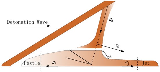
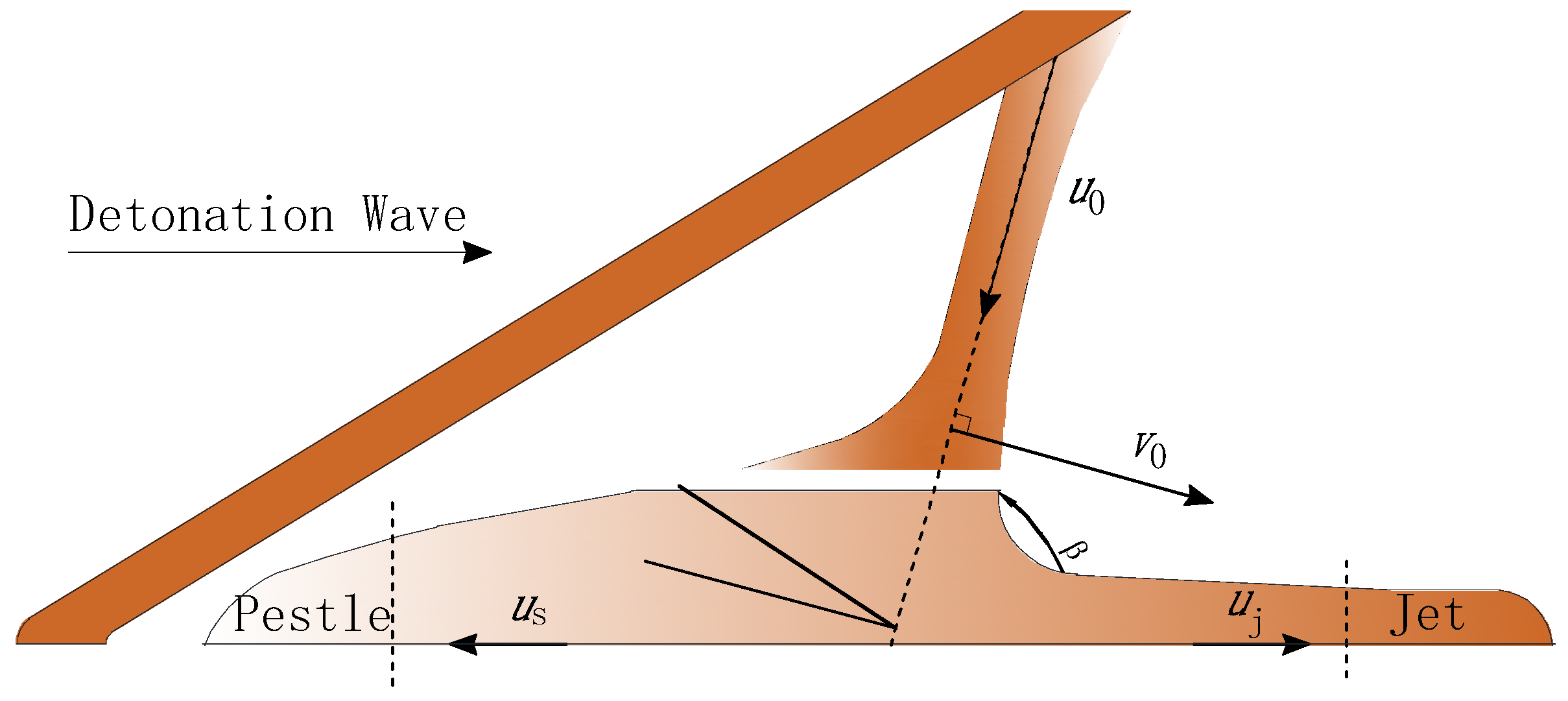
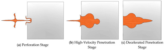
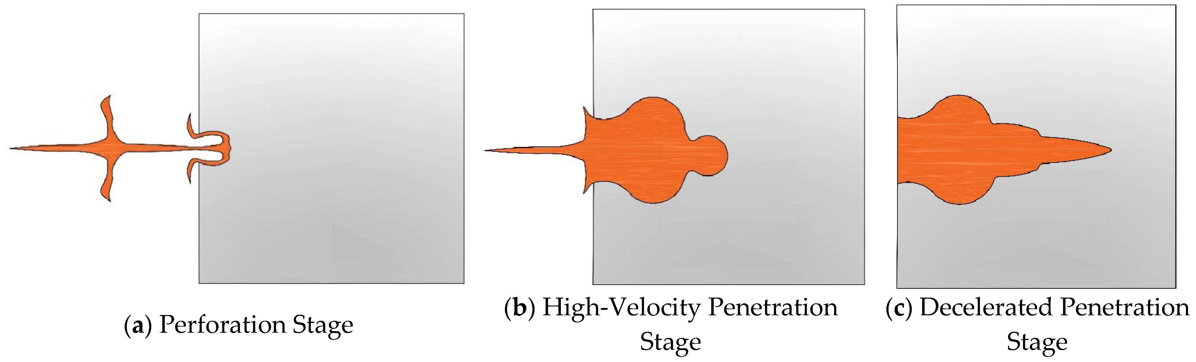
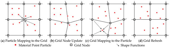
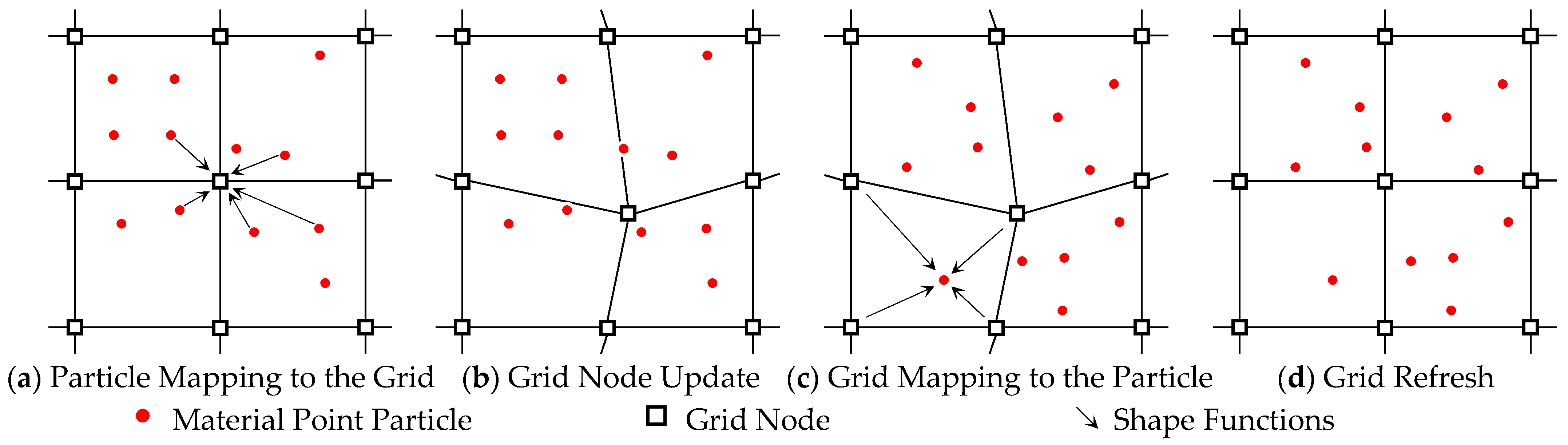
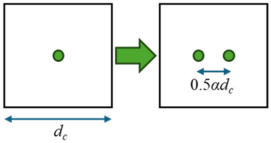
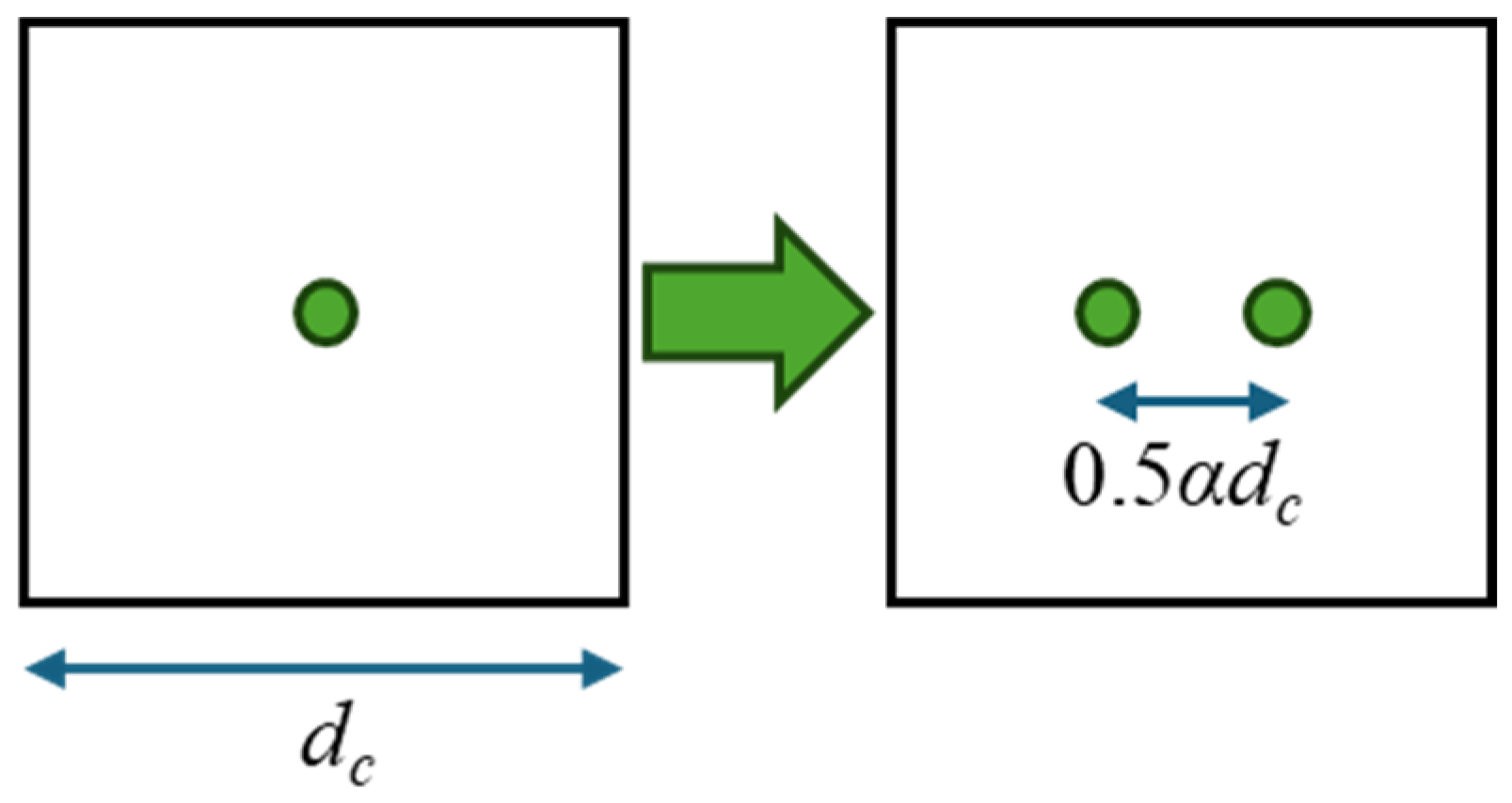
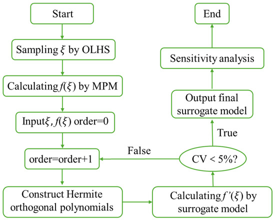
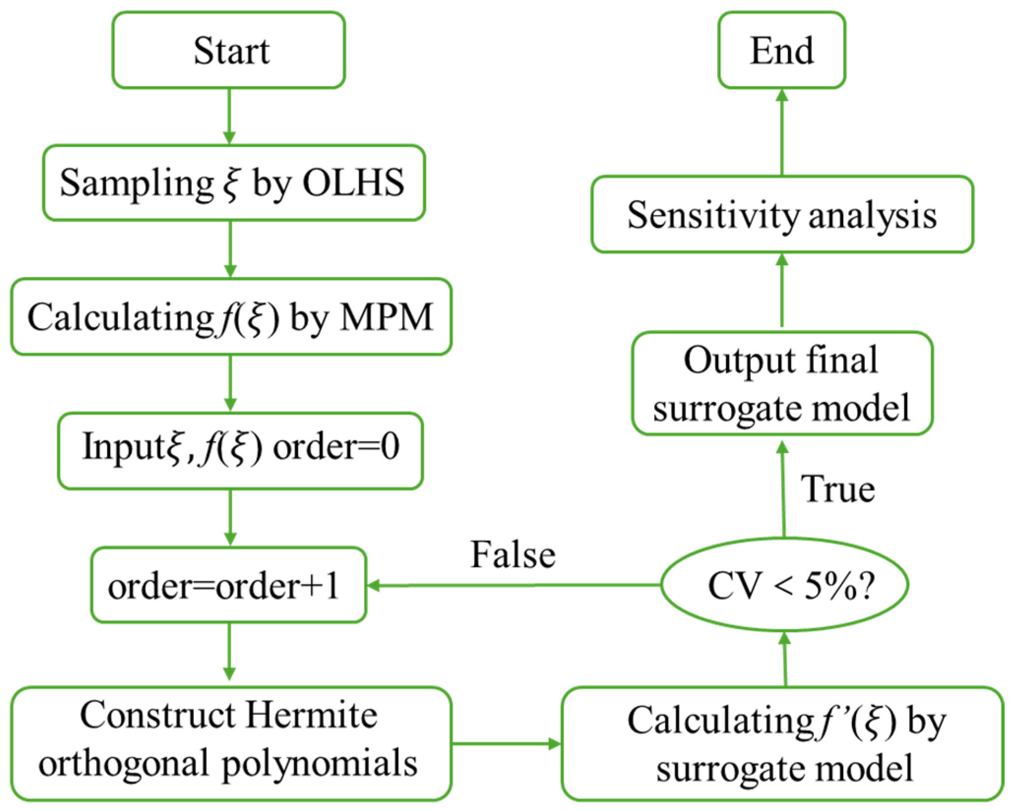
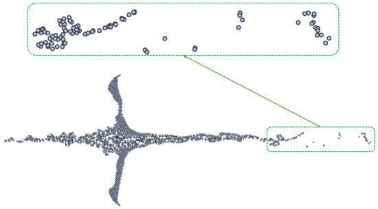
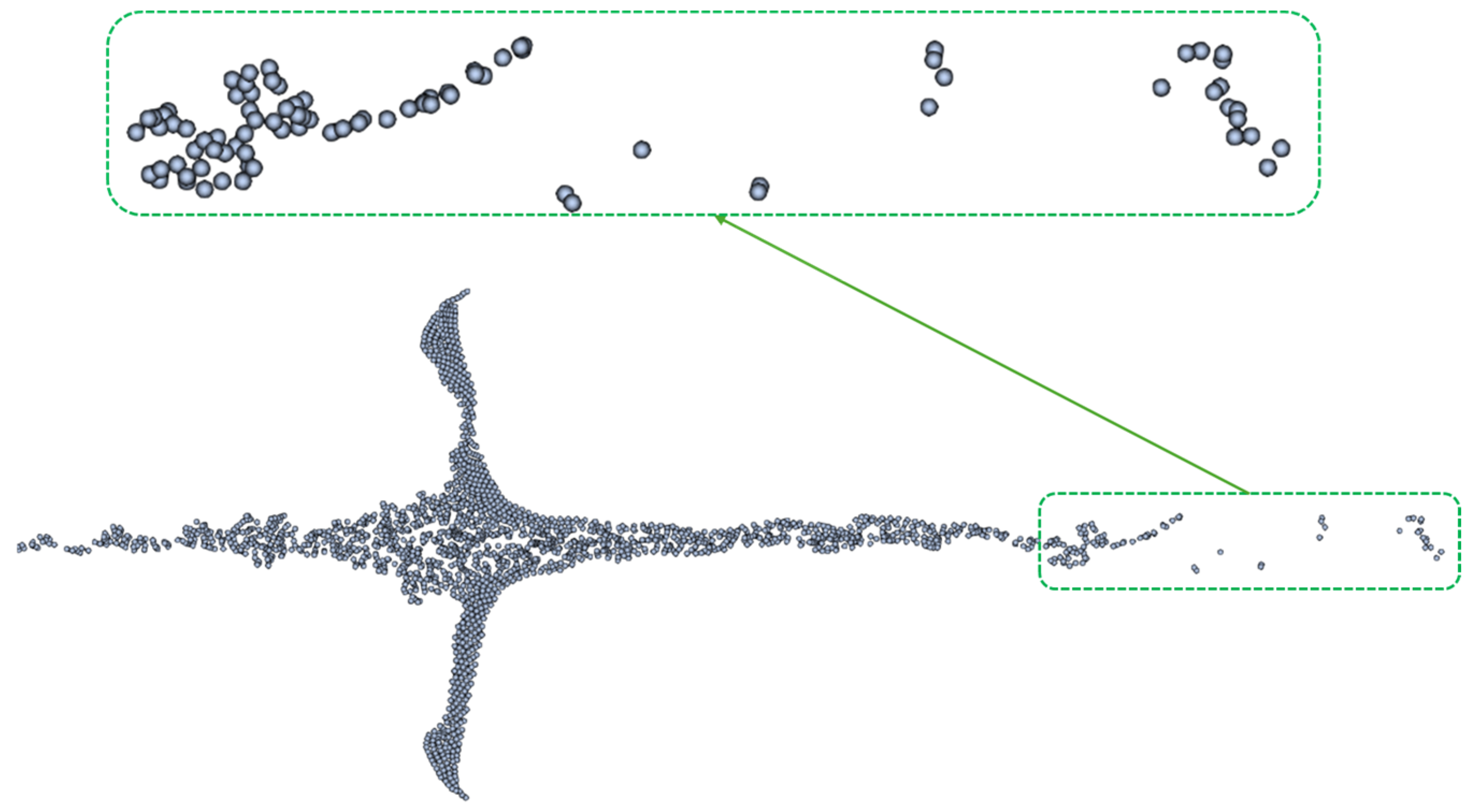
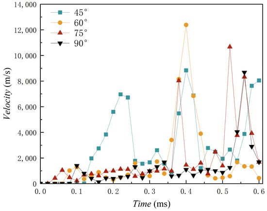
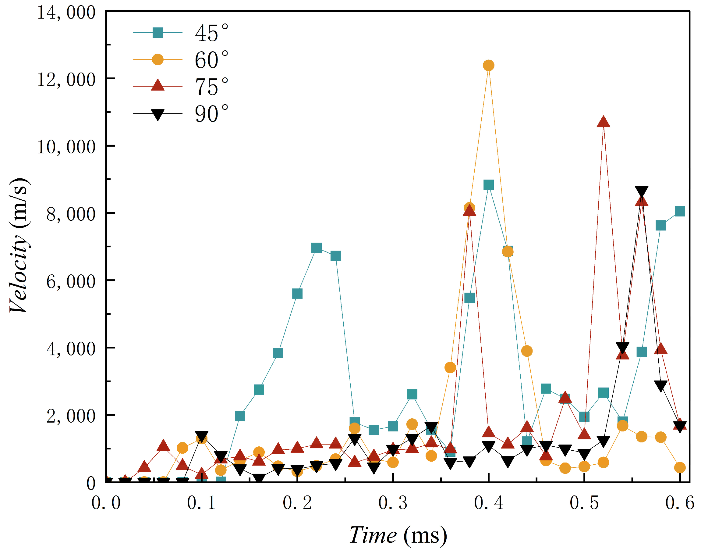
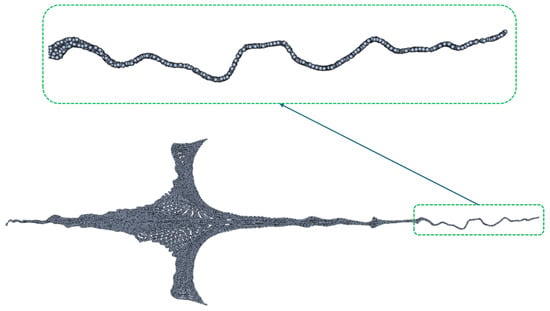
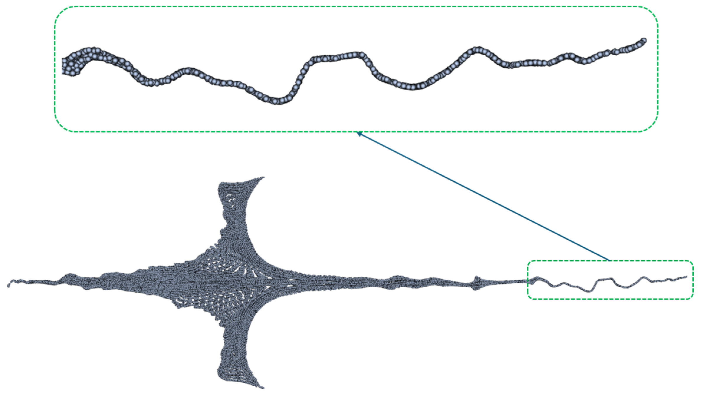
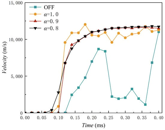
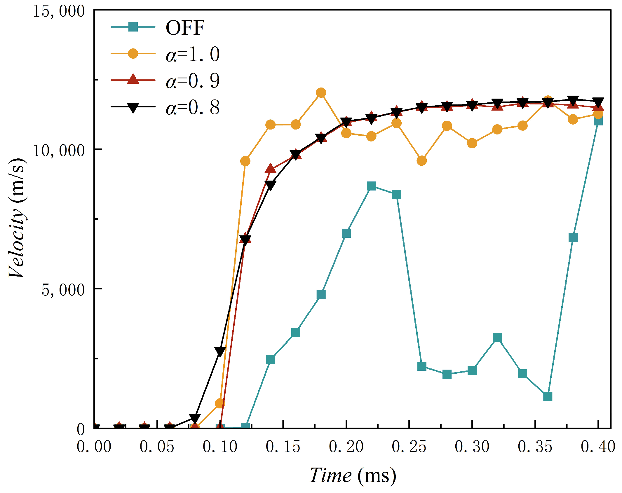
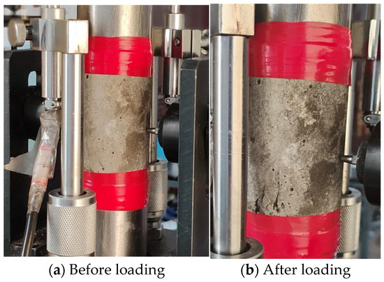
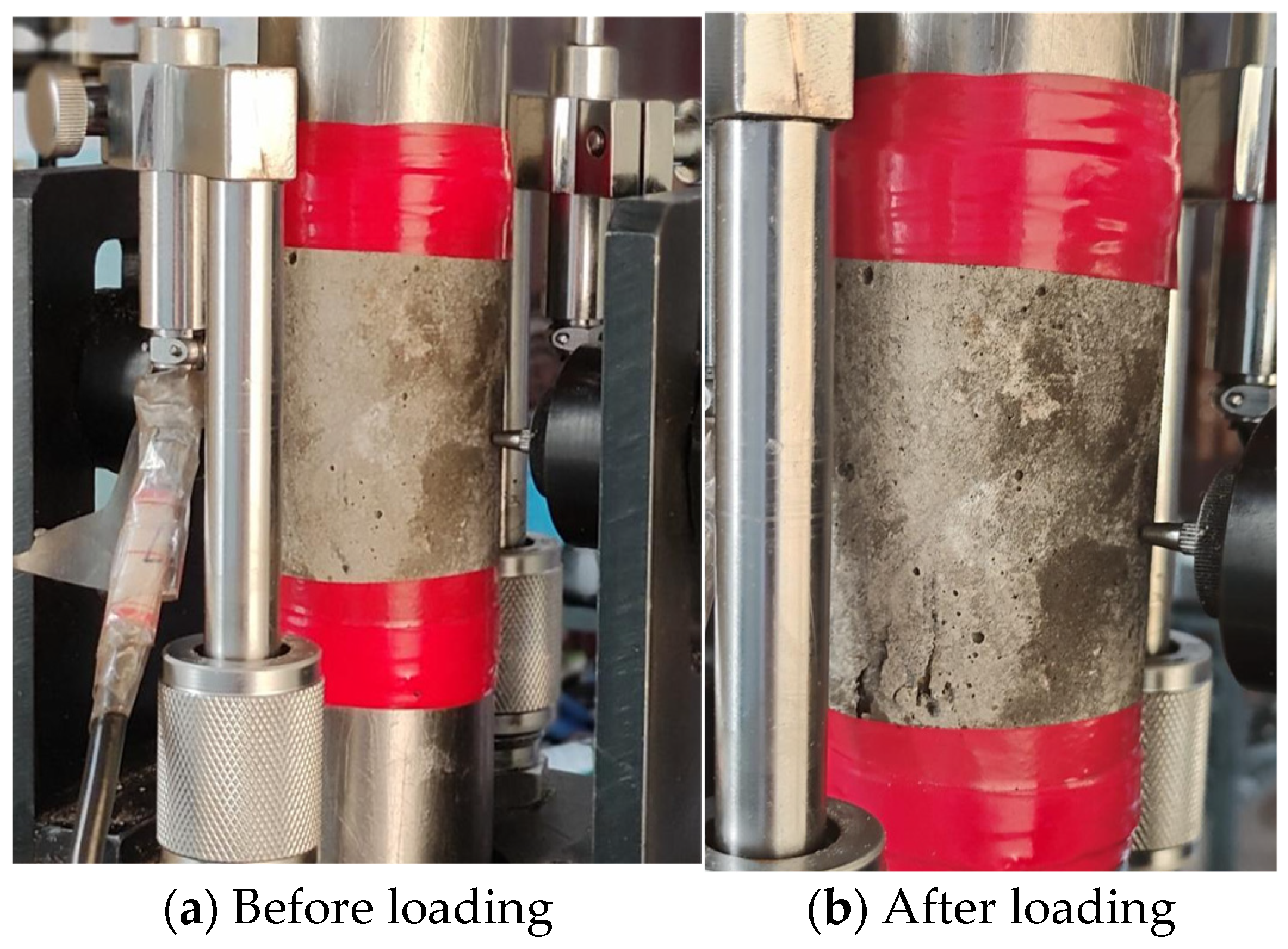
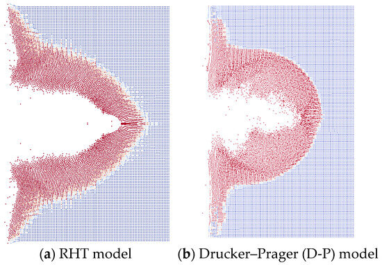
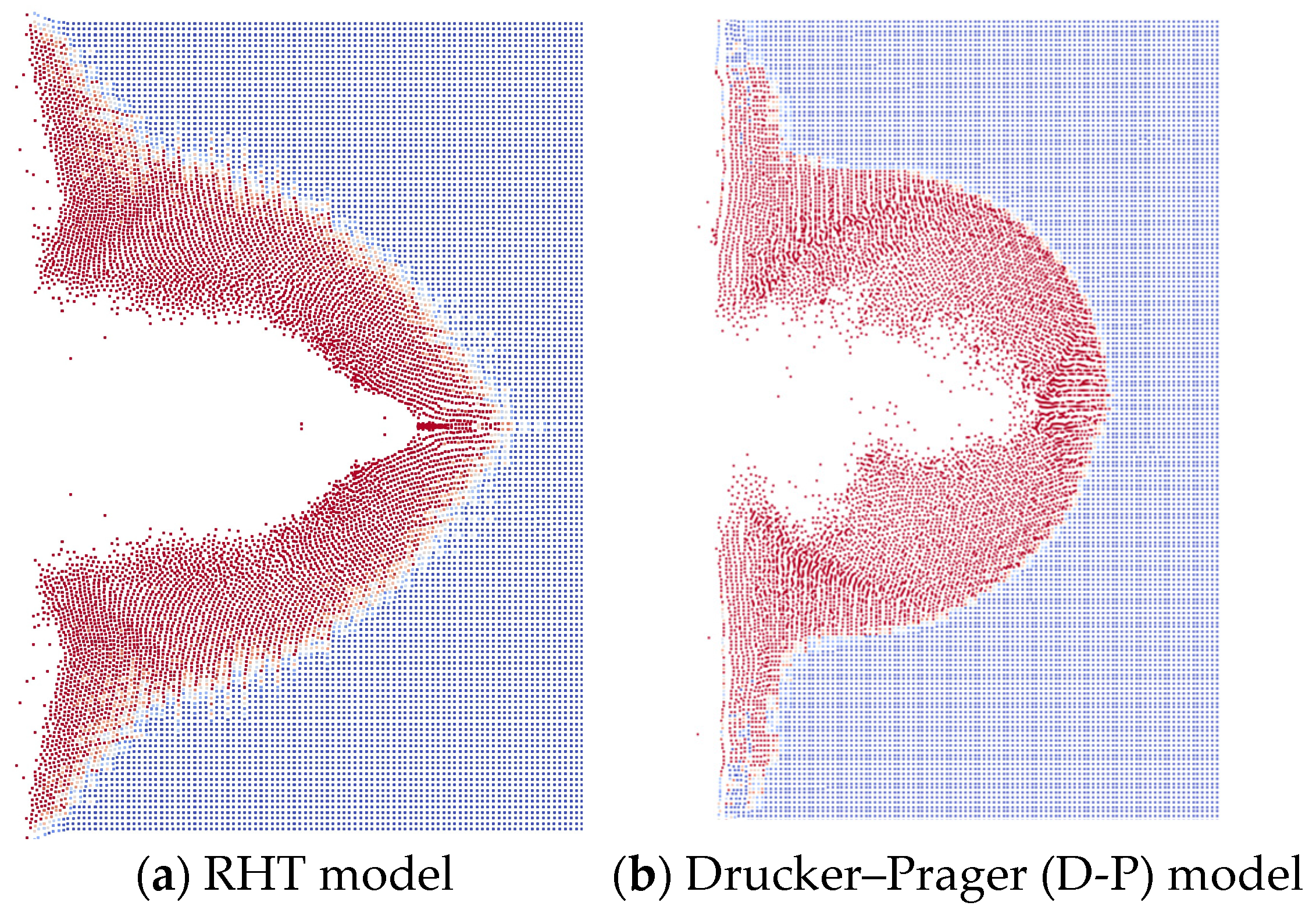
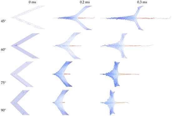
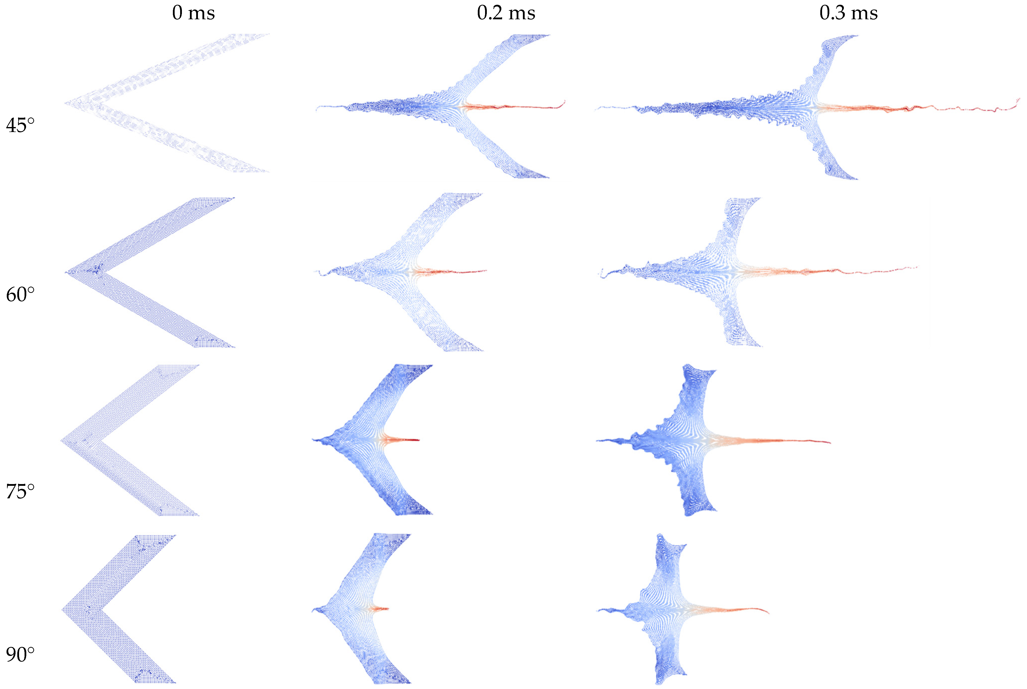
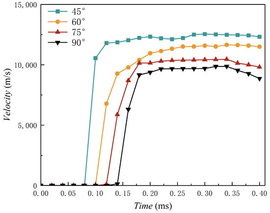
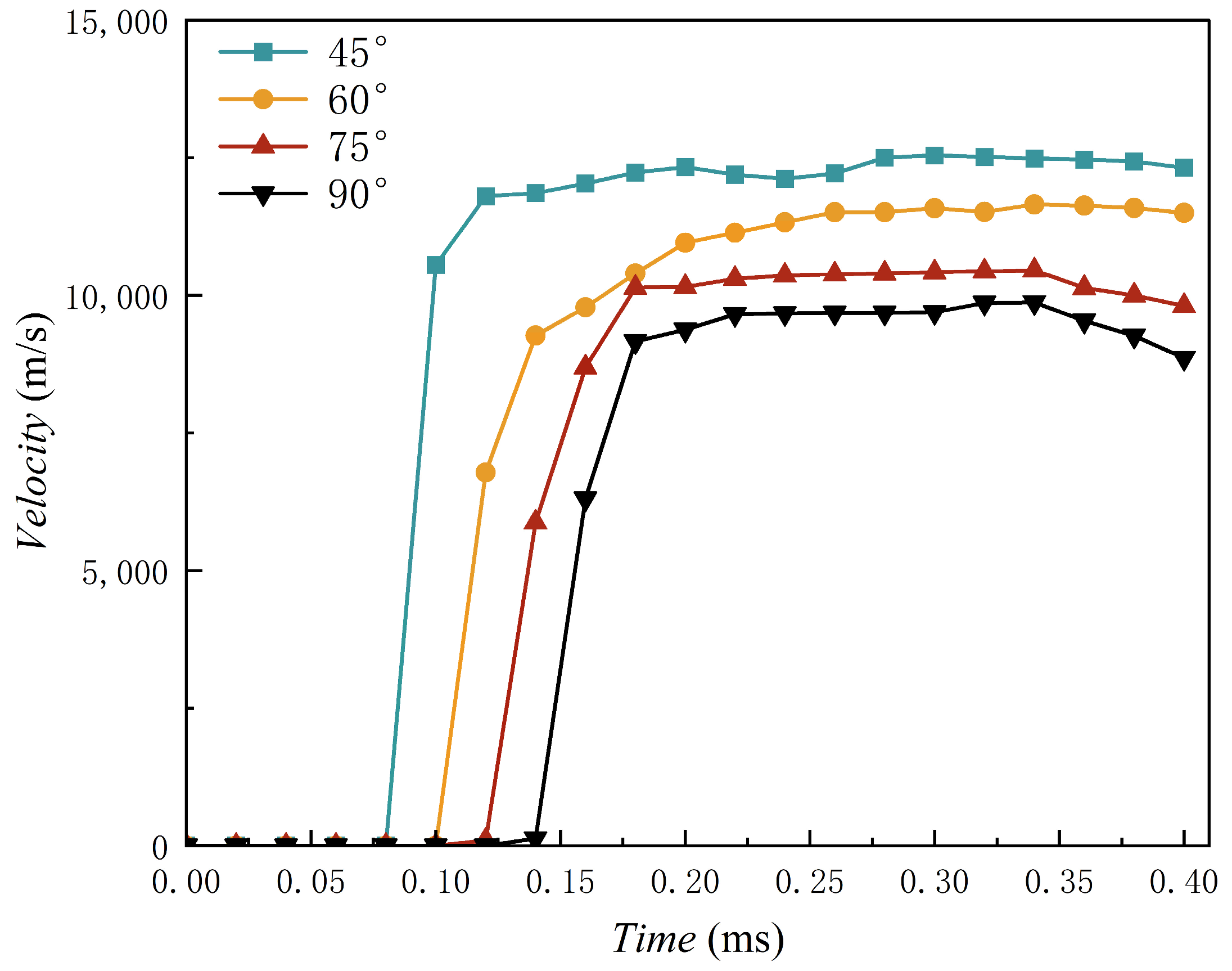
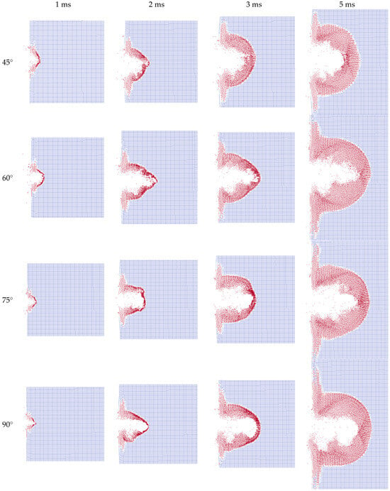
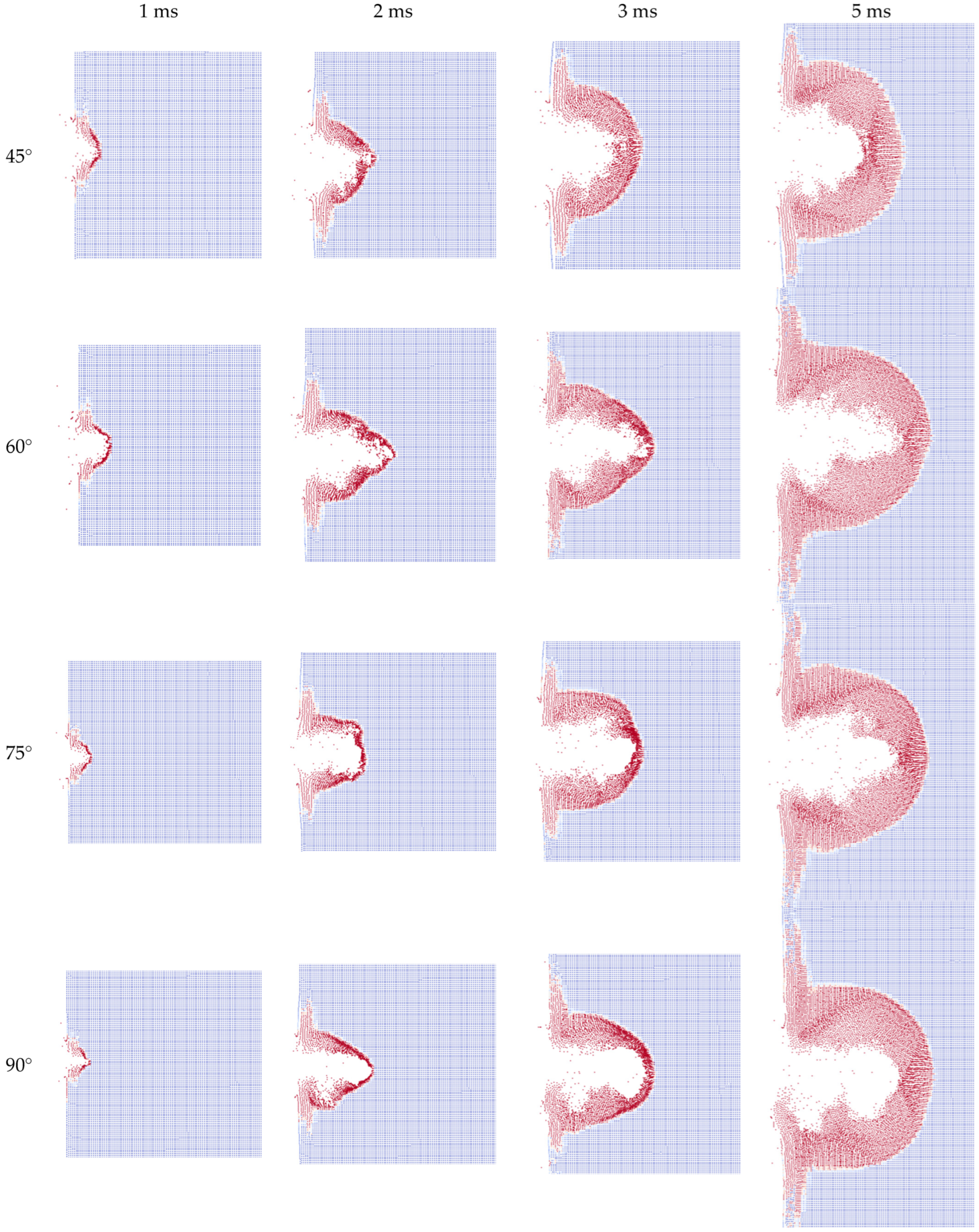
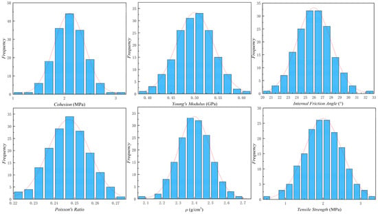
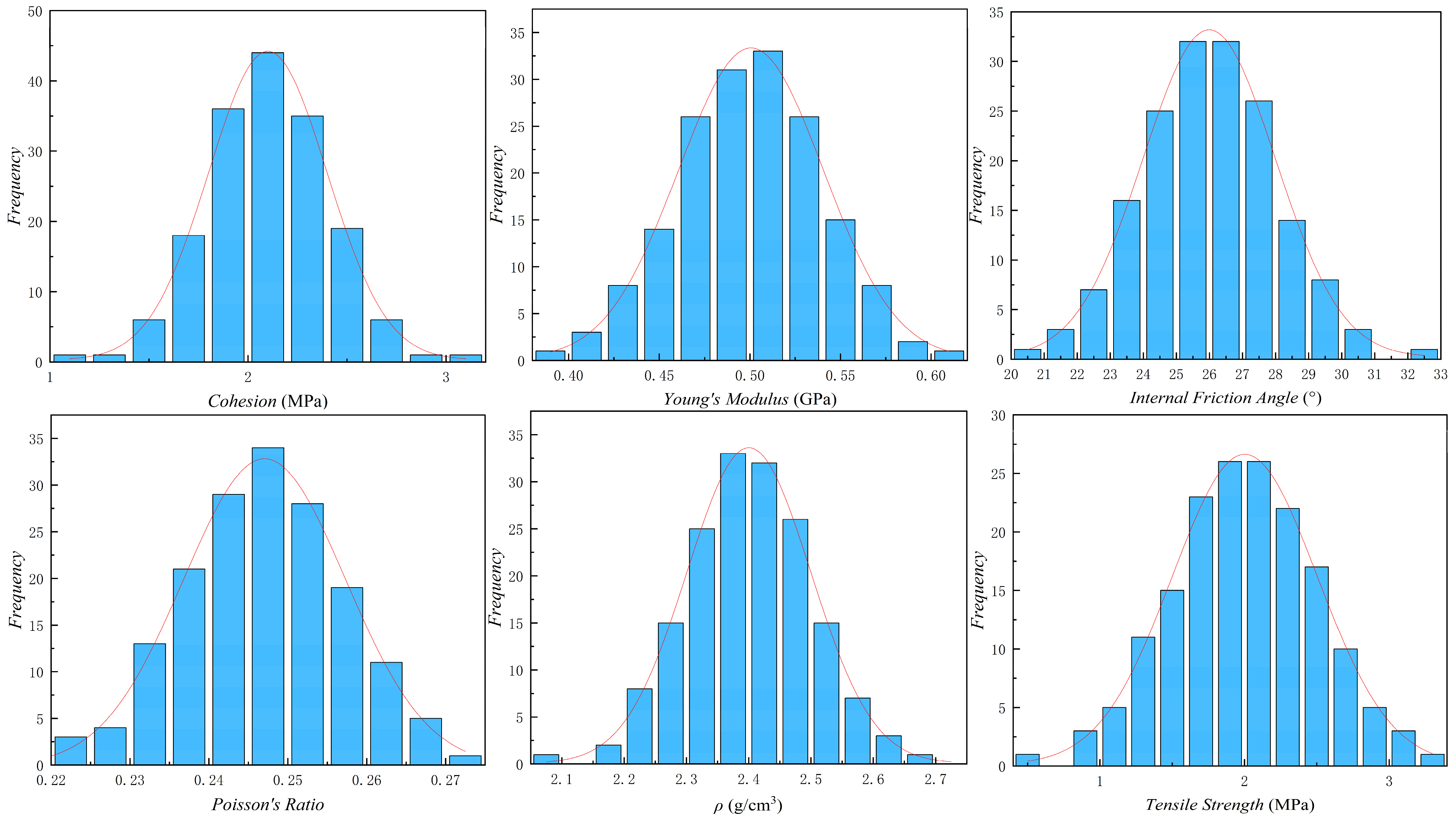
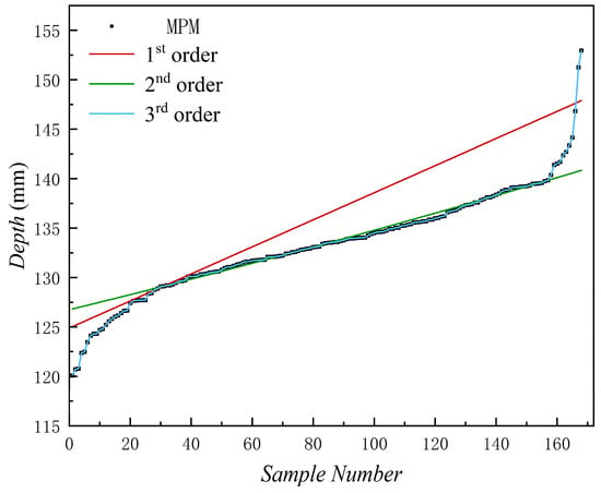
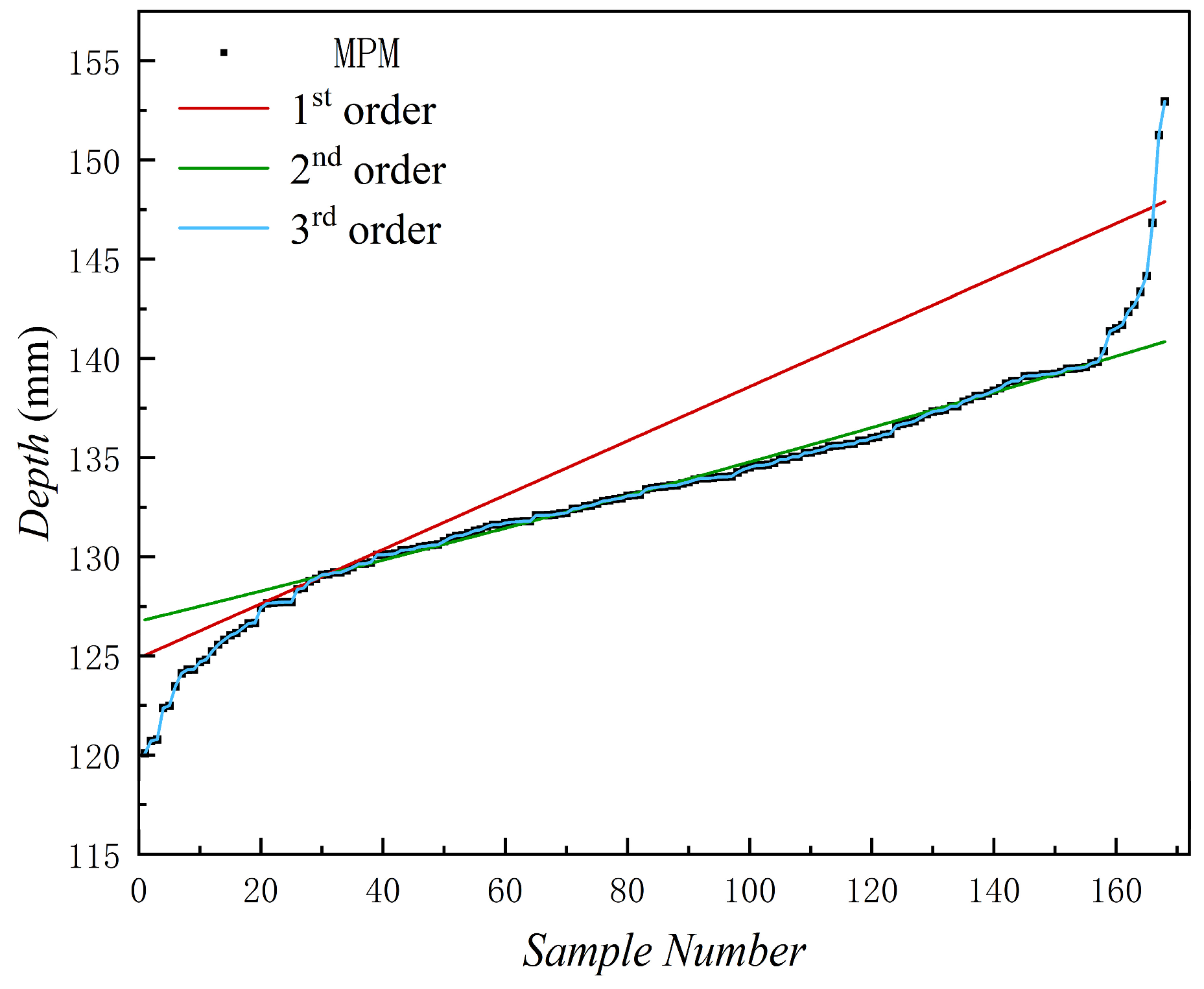
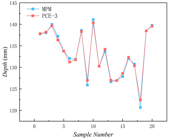
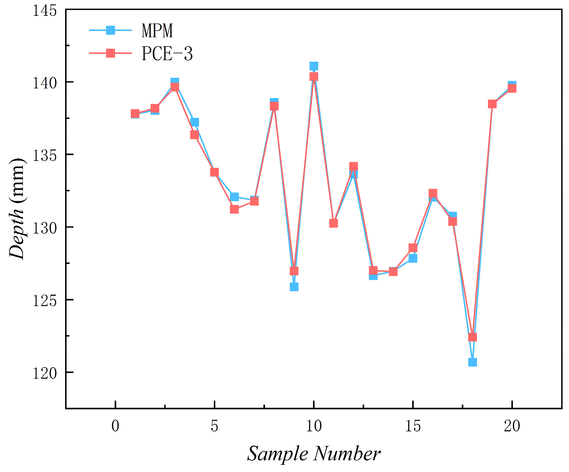
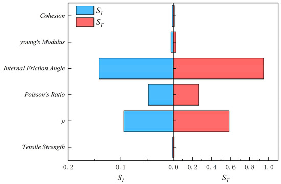
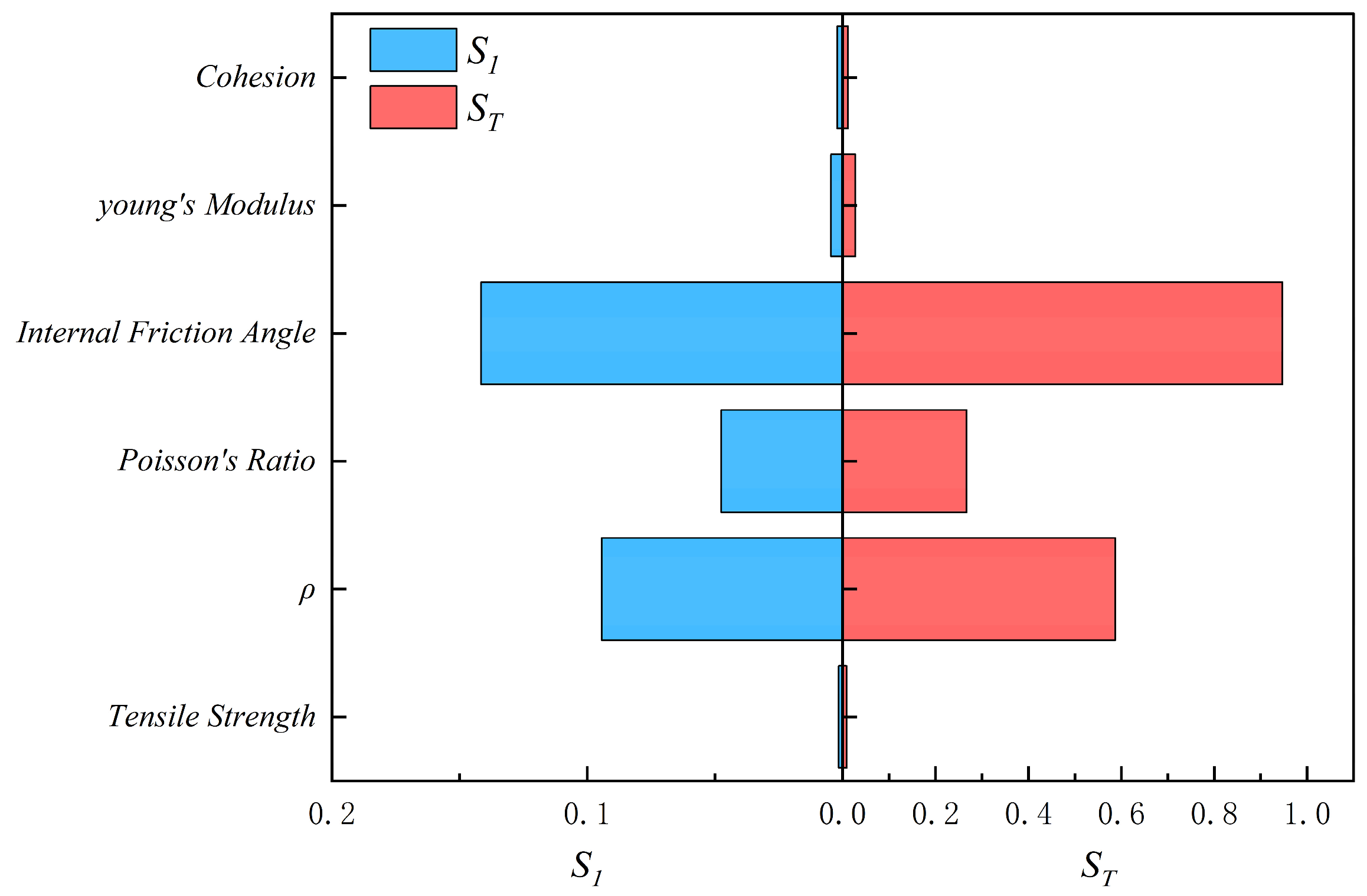
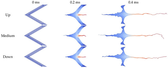
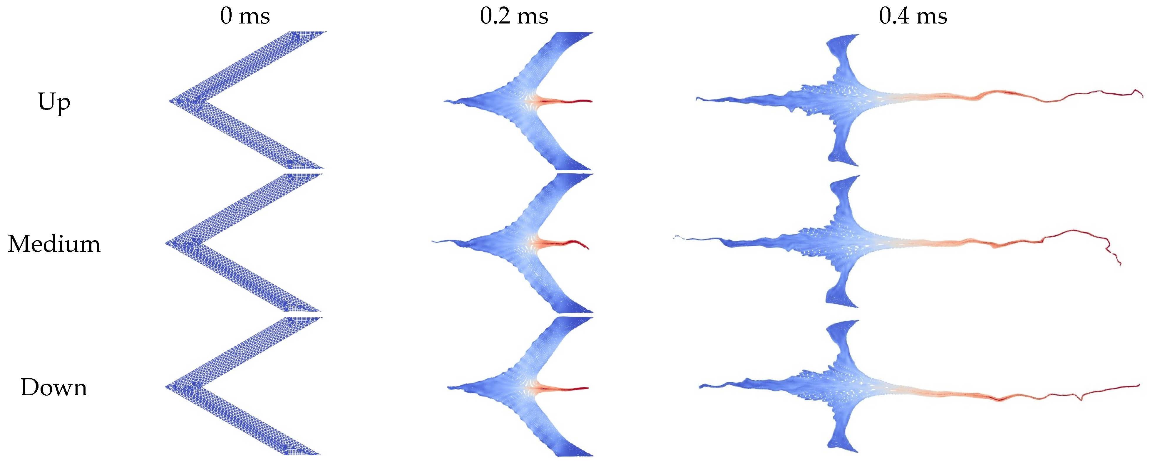
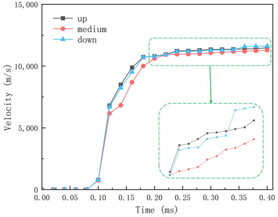
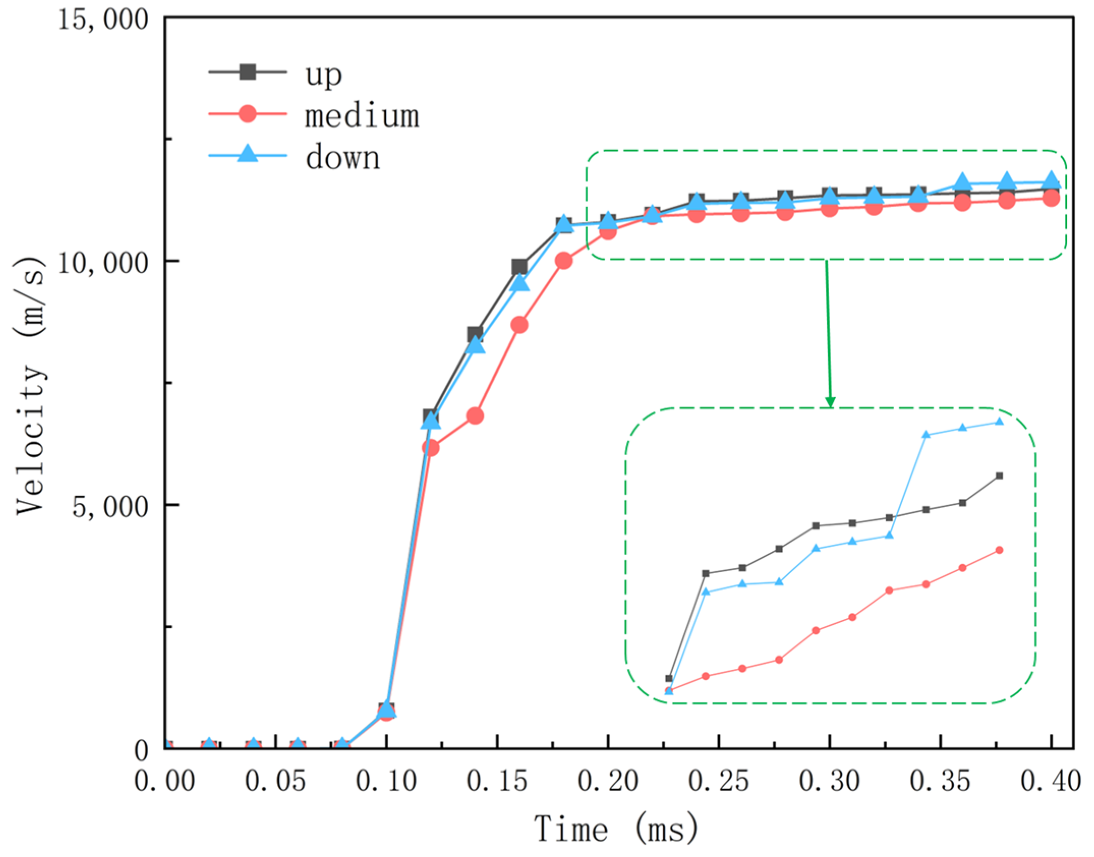
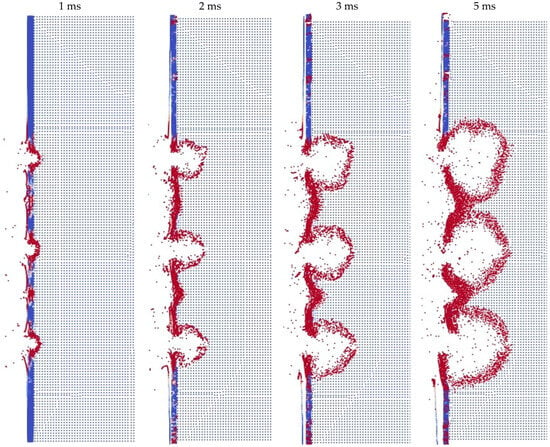
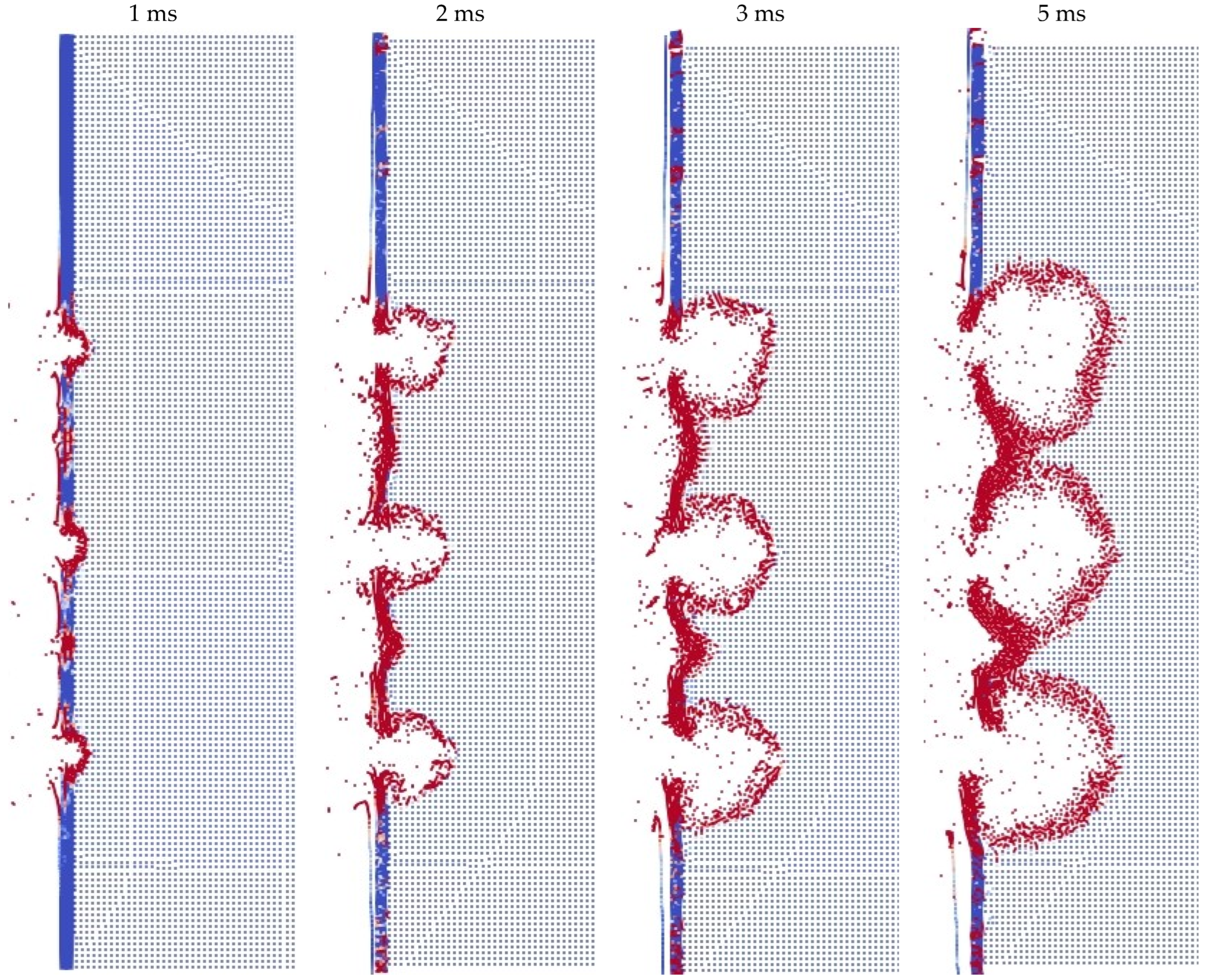
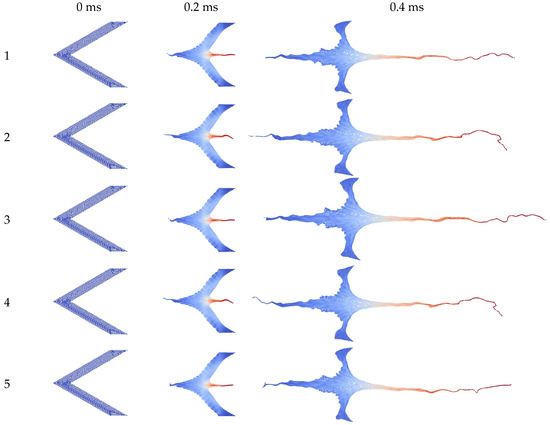
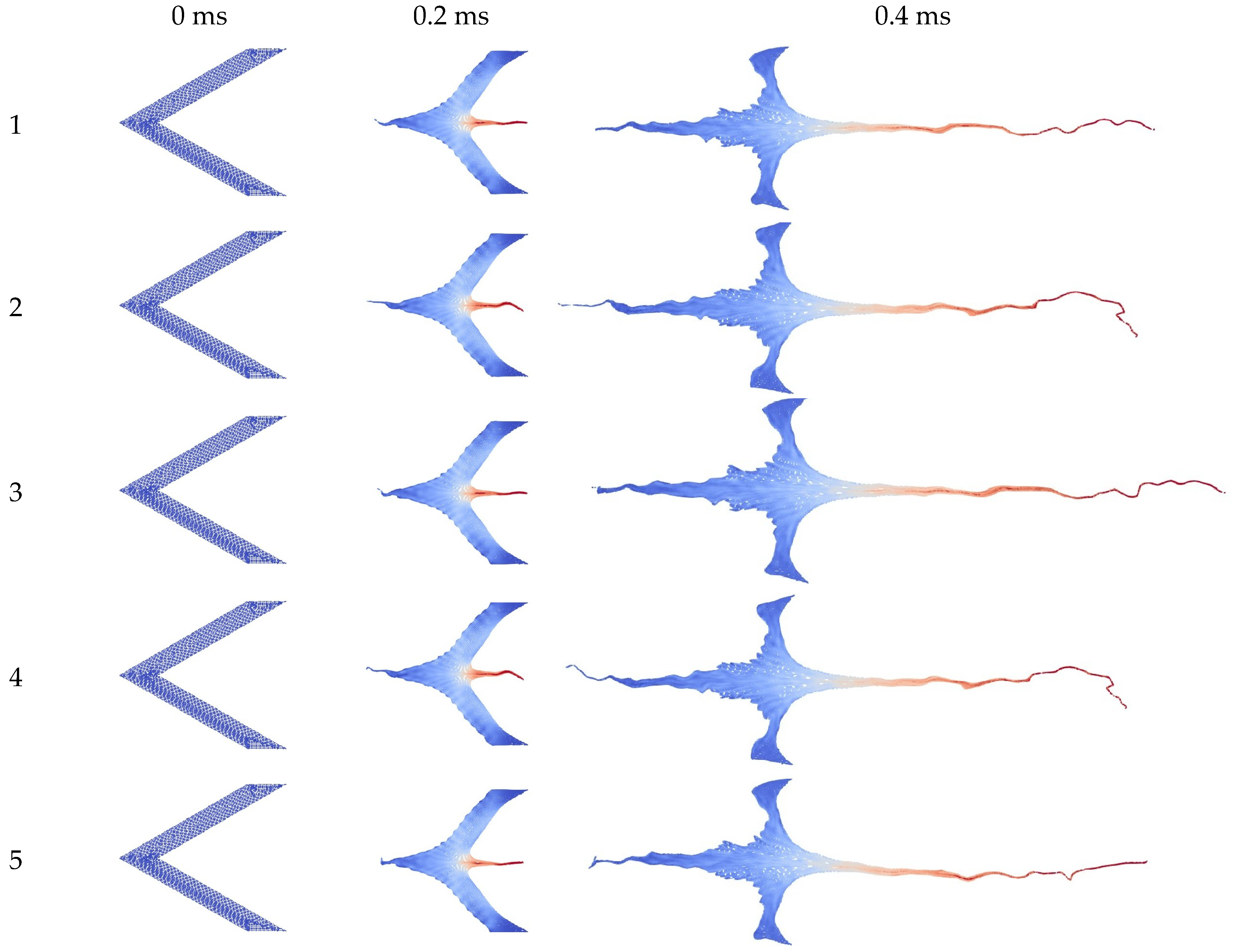
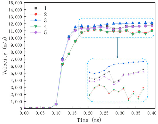
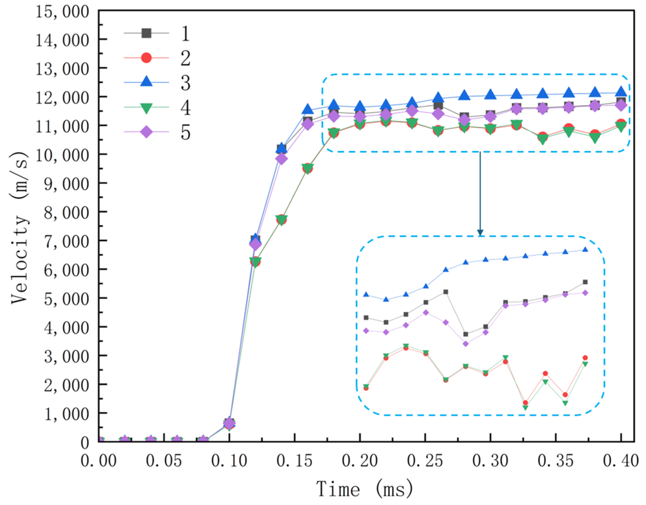
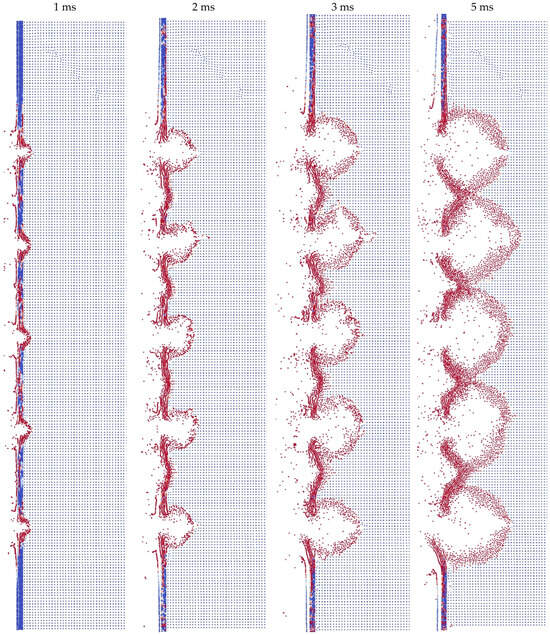
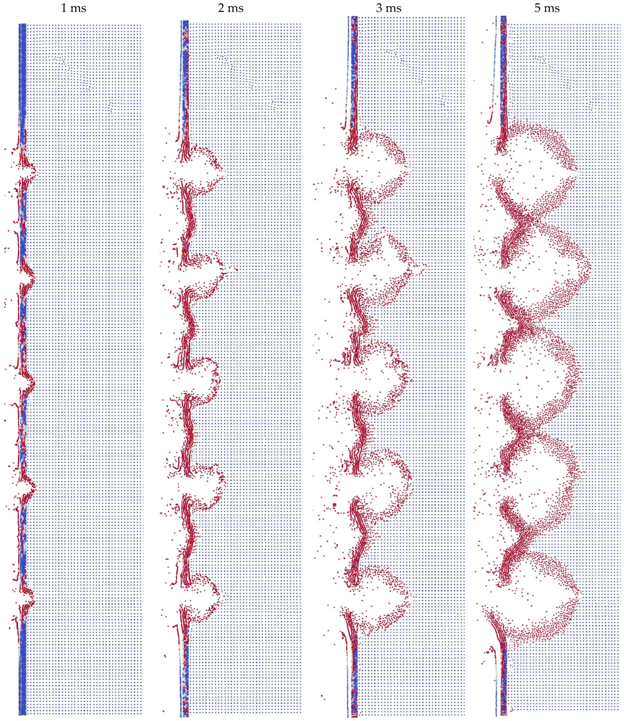
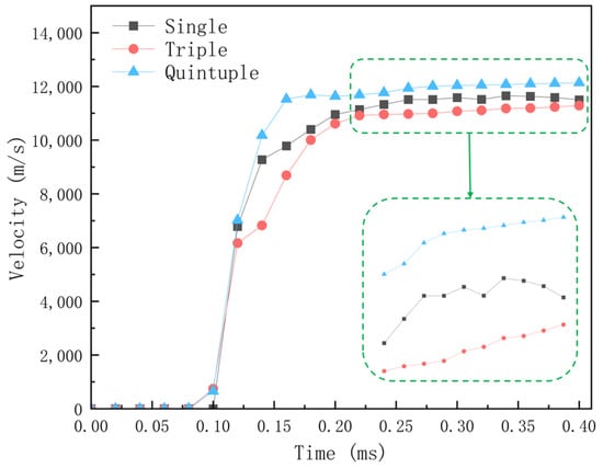
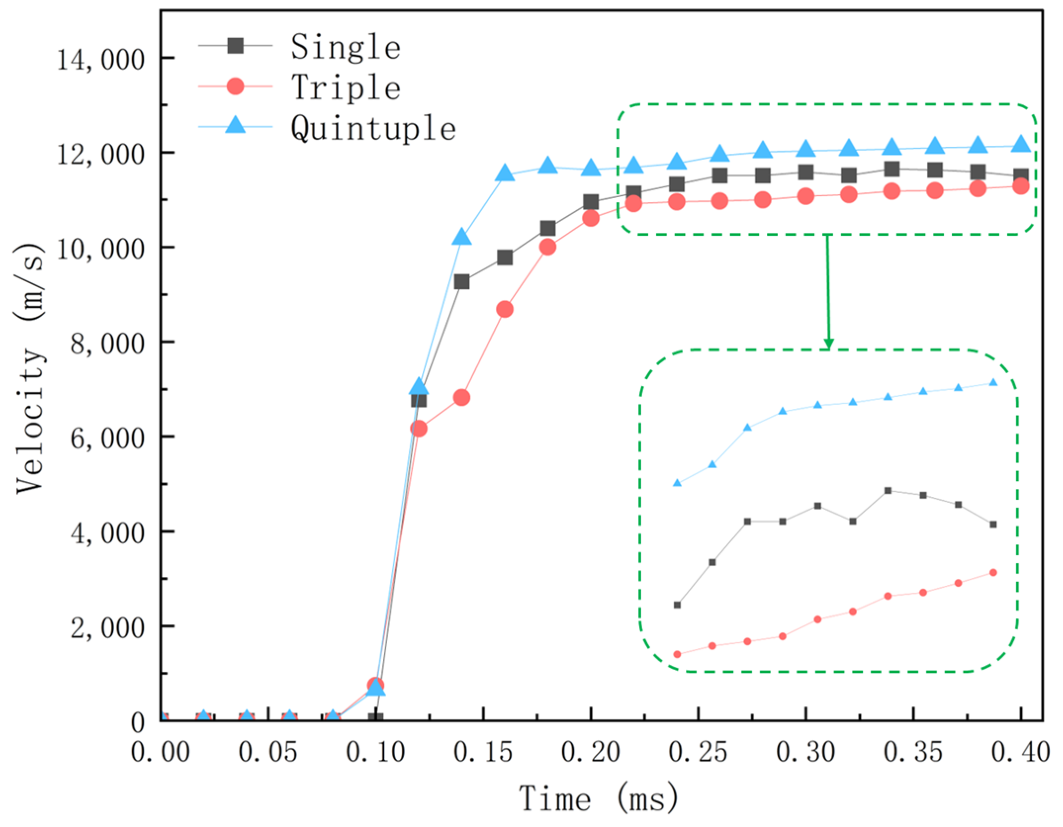
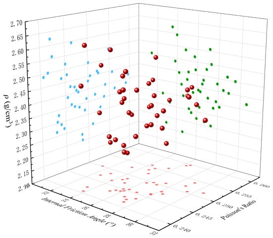
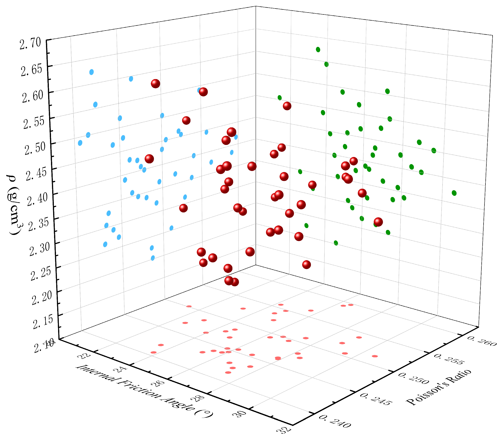
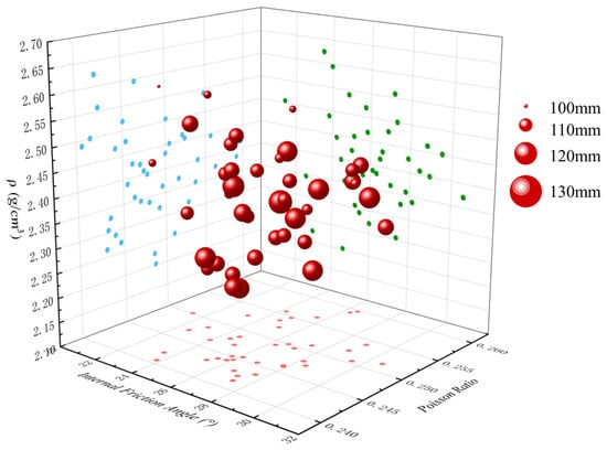
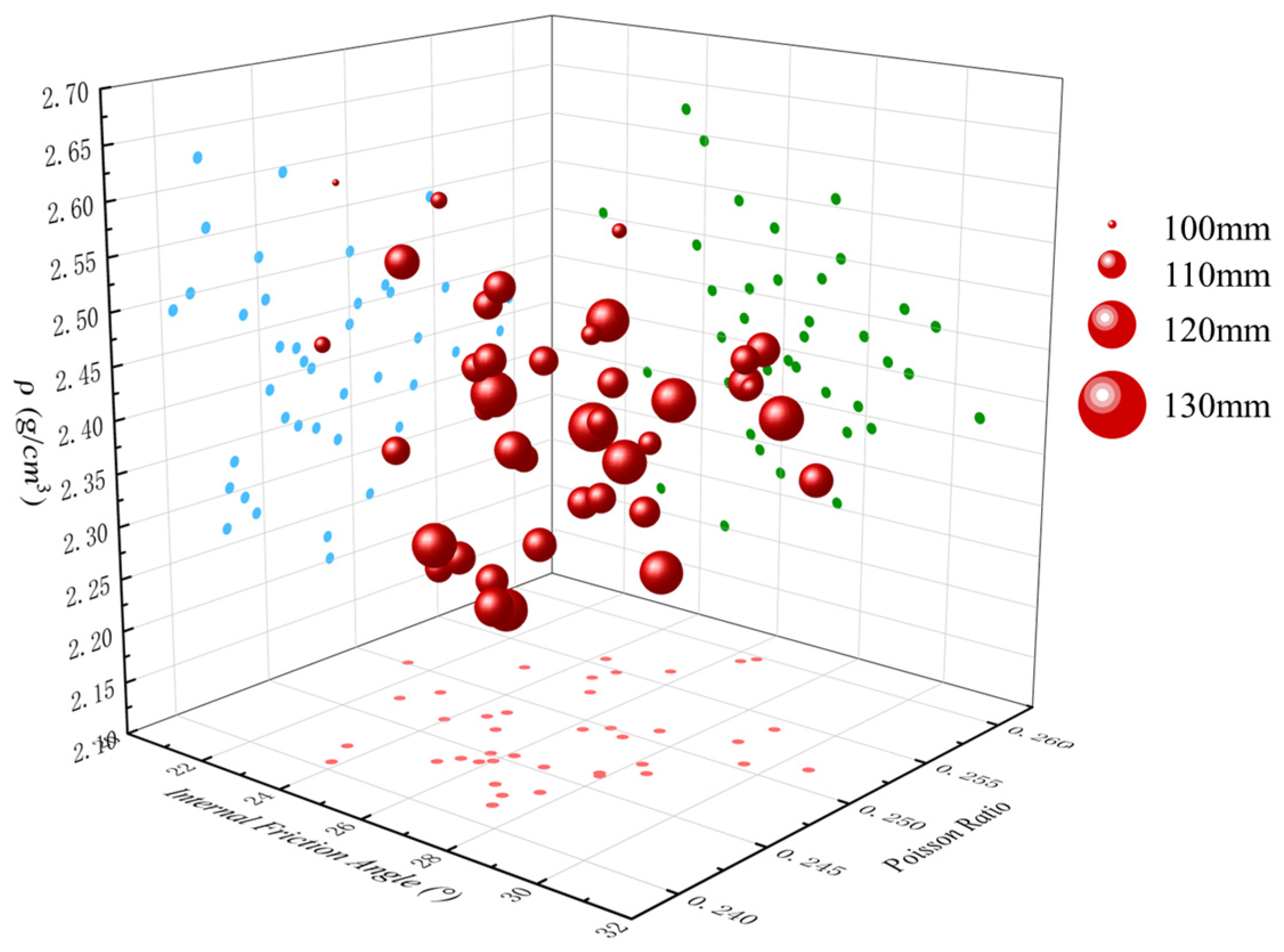
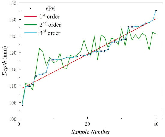
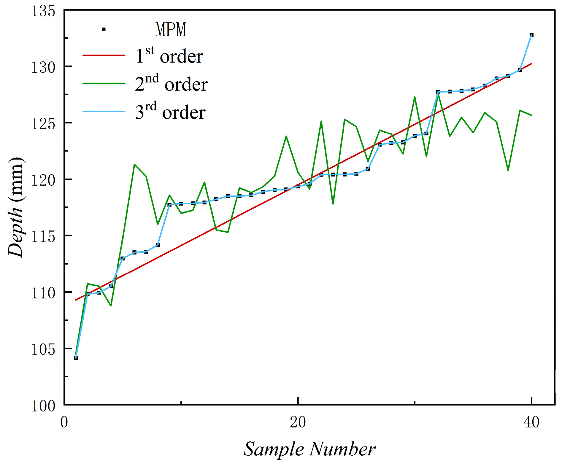
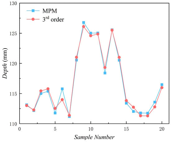
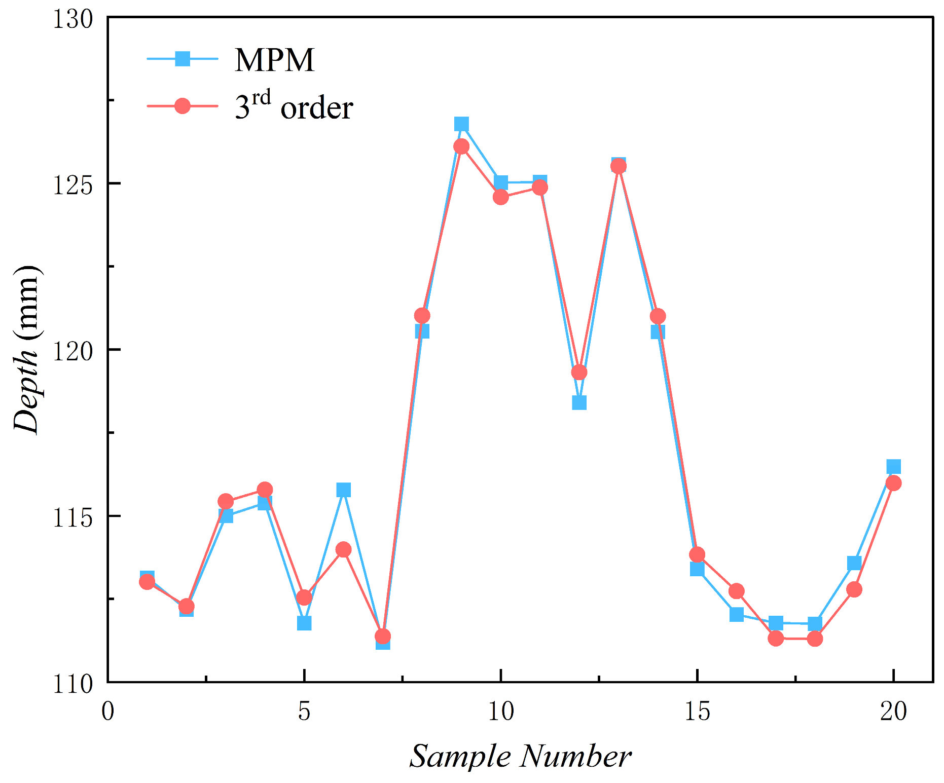
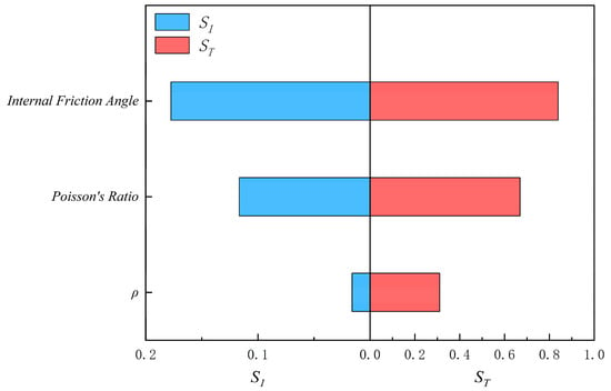
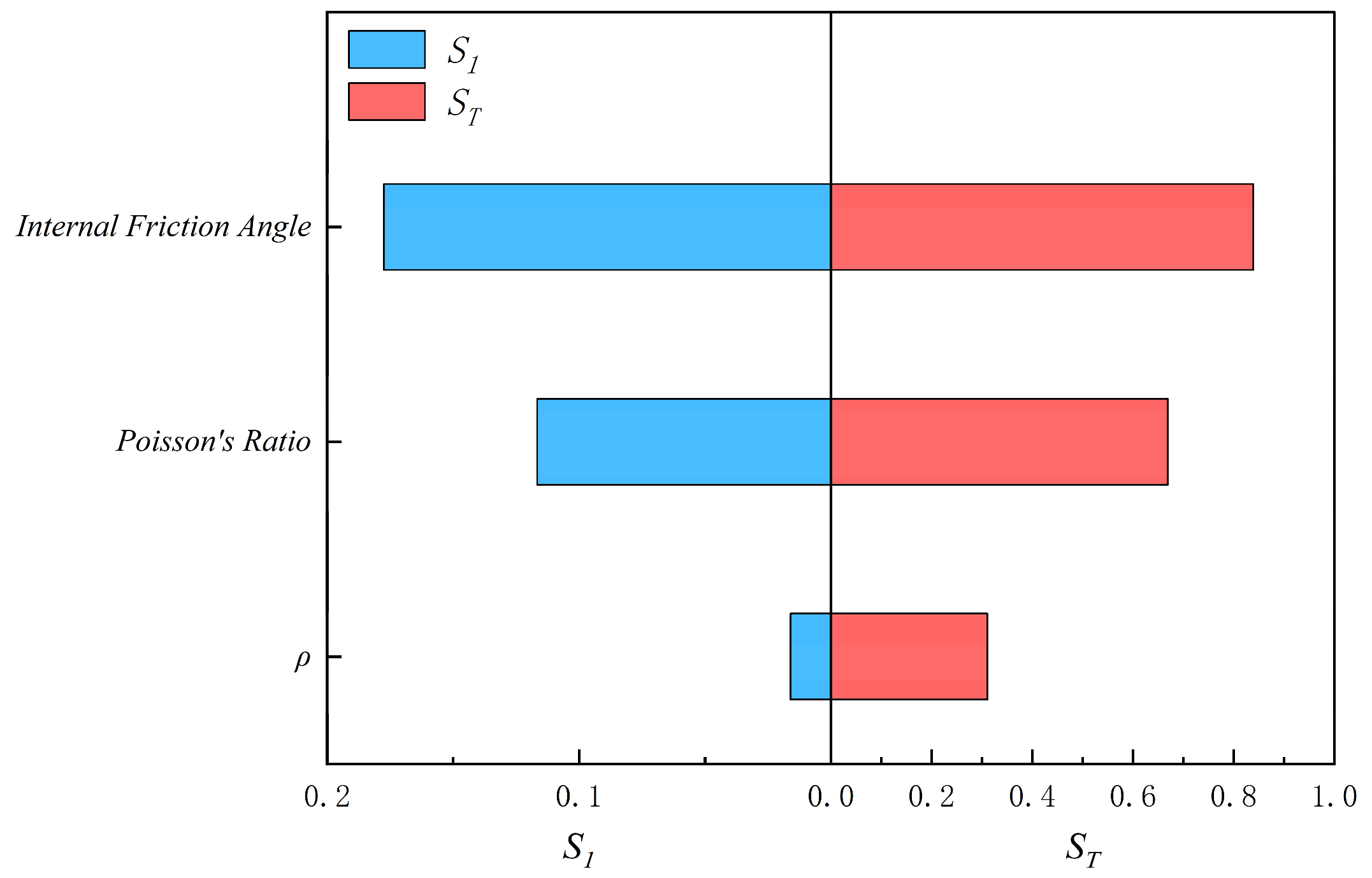
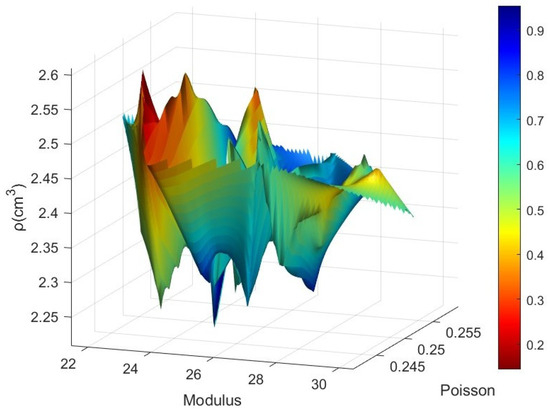
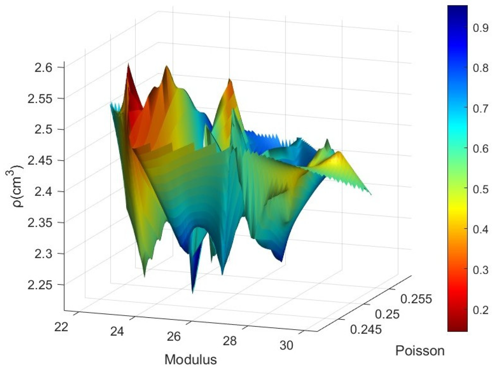

Disclaimer/Publisher’s Note: The statements, opinions and data contained in all publications are solely those of the individual author(s) and contributor(s) and not of MDPI and/or the editor(s). MDPI and/or the editor(s) disclaim responsibility for any injury to people or property resulting from any ideas, methods, instructions or products referred to in the content. |
© 2026 by the authors. Licensee MDPI, Basel, Switzerland. This article is an open access article distributed under the terms and conditions of the Creative Commons Attribution (CC BY) license.