Productivity Prediction in Tight Oil Reservoirs: A Stacking Ensemble Approach with Hybrid Feature Selection

Abstract

To address the challenges of low accuracy and complex influencing factors in predicting horizontal well fracturing productivity during the development of unconventional oil and gas resources such as tight oil, this paper proposes a productivity prediction framework based on an improved feature selection method and an ensemble learning model. This study employs a fusion analysis using the entropy weight method to combine Pearson correlation analysis and improved gray relational analysis (IGRA) for feature selection. Thirteen machine learning models were tested with six distinct parameter combinations to construct a Stacking-based ensemble learning model, with base models including Random Forest (RF), Ridge Regression (RR), and Artificial Neural Network (ANN). Particle Swarm Optimization (PSO) was employed to optimize hyperparameters, followed by interpretability analysis using SHapley Additive exPlanations (SHAP). The results indicate that the model with fused weights demonstrated optimal performance. The Stacking model achieved significantly improved accuracy after PSO optimization, with the coefficient of determination increasing by 4.9%, outperforming all comparison models. Engineering guidance is provided: Under current geological conditions, sand ratio and displacement fluid volume require fine-tuning to prevent over-treatment. Fracturing design should implement differentiated strategies based on the target sand body thickness. This study not only delivers a high-precision production prediction tool but also offers decision support for efficient unconventional oil and gas field development through its exceptional interpretability.

1. Introduction

Petroleum occupies an indispensable position in the global energy supply and holds an irreplaceable role within the energy system. As global energy demand continues to grow and reserves of conventional energy sources become increasingly depleted, the development of unconventional oil and gas resources has become a strategic priority for ensuring energy security [1,2,3,4]. Among these, tight oil resources, with their enormous potential, are gradually emerging as the core successor field for global oil and gas production growth [5,6]. Such reservoirs typically exhibit poor physical properties, significant heterogeneity due to natural fracture development, and low natural productivity [7]. Currently, fracturing technology has become a crucial method in oil and gas extraction, particularly for tight reservoir development [8,9]. The integration of horizontal wells and fracturing technology can significantly enhance reservoir recovery rates and increase productivity [10]. However, horizontal well fracturing faces numerous challenges in practical application. A core challenge lies in accurately predicting post-fracturing productivity [11,12]. The complexity of productivity forecasting is significantly heightened due to multiple influencing factors, including geological characteristics, fracturing design, and well placement. Throughout this process, the optimization of fracturing parameters, reservoir heterogeneity, and the interaction between well placement and the reservoir all exert profound impacts on production outcomes. Therefore, effectively integrating geological, engineering, and production data while employing scientific predictive models to accurately forecast productivity has become crucial for enhancing oilfield development efficiency and plays a vital role in guiding oil and gas production [13].

The evaluation and prediction of factors affecting productivity represent one of the major challenges in oilfield development [14,15]. Conventional prediction methods primarily include analytical methods [16,17], empirical methods [18,19], production decline analysis [20,21], and numerical simulation methods [22,23]. Hu et al. [24] employed numerical modeling and power-law decline models to study production forecasting and influencing factors for fractured horizontal wells in tight reservoirs, validating their findings against actual production data. Sun et al. [25] developed a semi-analytical model for tight reservoirs containing microfractures, analyzing the impact of microfractures on horizontal well production and identifying key parameters through sensitivity studies. MoradiDowlatabad et al. [26] combined statistical algorithms with numerical simulation to evaluate parameter influences in multistage fractured horizontal well design, proposing an optimization method that was based on production stages. Li et al. [27] developed a vector production prediction model by integrating start-up pressure characteristics and coupled effects of dissolved gas flow to describe oil–gas separation behavior in low-permeability tight reservoirs. Xu et al. [28] developed a three-dimensional discrete random fracture network model that integrates microseismic data with natural fracture properties to achieve detailed characterization of fracture networks and horizontal wells. By coupling stress sensitivity with fluid flow simulation, they effectively analyzed the impact of different fracture parameters on productivity. Although these methods have achieved certain successes in different scenarios, they still exhibit significant limitations: Power-law decay models can match steady-state production data but poorly adapt to unsteady production systems, with long-term predictions potentially deviating from reality; analytical models account for fracture effects but still oversimplify complex flow mechanisms. Discrete models achieve refined characterization of fracture networks but inadequately consider the time-varying effects of fracture flow-conductivity. Numerical simulations and statistical methods can evaluate multi-parameter synergistic effects but rely heavily on objective function selection and incur high computational costs. These limitations have driven researchers toward data-driven approaches like machine learning to more efficiently address the nonlinear, high-dimensional challenges in unconventional oil and gas production forecasting [29].

With the advancement of artificial intelligence technology, machine learning methods offer new possibilities for accurately predicting oil and gas field production, enabling efficient development [30,31]. Liu et al. [32] developed a production forecasting system based on reservoir classification for both conventional and unconventional reservoirs. By employing seven machine learning algorithms, including extreme gradient boosting (XGB) and calculating the effective thickness, they improved prediction accuracy by 10%. Ning et al. [33] systematically compared the performance of Auto-Regressive Integrated Moving Averages (ARIMA), Long Short-Term Memory (LSTM), and Prophet time series models in tight reservoirs of the U.S. DJ Basin. They found that LSTM and ARIMA excelled at capturing production fluctuation characteristics: LSTM effectively learned long-term dependencies, while ARIMA demonstrated strong cross-well transfer prediction capabilities. Lu et al. [34] developed a deep neural network-PSO-coupled framework to optimize shale oil fracturing parameters, achieving a cumulative oil production increase of 2969 m³ in practical applications. Tong et al. [35] applied the XGB algorithm to predict productivity in China’s terrestrial tight oil reservoirs. Feature importance analysis confirmed the decisive influence of fracturing parameters on initial productivity. Ng et al. [36] innovatively combined the PSO algorithm with support vector regression (SVR) and neural networks, achieving high-precision predictions with R² > 0.94 in Norway’s Volve oilfield. Pan et al. [37] proposed a combined model with the convolutional neural network (CNN), LSTM neural network, and the self-attention mechanism (SA), and the hybrid model outperformed traditional methods in both production trend and numerical prediction through spatio-temporal feature extraction and self-attention mechanisms. However, despite demonstrating significant potential in predictive accuracy, these data-driven approaches face several critical challenges: models often operate as “black boxes”, with a lack of interpretability hindering their potential to reveal underlying physical mechanisms; high dependence on data quality and quantity limits generalization capabilities in data-scarce regions. Furthermore, most studies fail to translate data-driven discoveries into explicit engineering guidance, diminishing their practical application value. Therefore, developing a predictive framework that combines high accuracy, high interpretability, and provides clear engineering insights has become an urgent research need.

To address the limitations of existing routine machine learning applications, which often rely on simple homogeneous ensembles and struggle with high-dimensional, heterogeneous geological data, this paper proposes a productivity forecasting method that integrates feature selection with heterogeneous ensemble learning, aiming to overcome the trade-off between accuracy and interpretability. We employ a dynamic normalization strategy for traditional GRA based on median absolute deviation and an adjustable resolution coefficient to address scale differences and outliers in complex geological data. Furthermore, we balance linear and trend correlations using an entropy-weighted Pearson–IGRA hybrid feature selection strategy, thereby enhancing the robustness of feature screening. A Stacking ensemble learning model optimized by the PSO algorithm is constructed to fuse the advantages of multiple algorithms and achieve optimal predictive performance. SHAP value analysis is employed to provide global and well-specific explanations for the optimized model, quantitatively revealing the contribution of each feature to productivity prediction, identifying complex phenomena, and translating predictive signals into differentiated and actionable fracturing strategies to prevent over-treatment.

2. Methodology

2.1. Correlation Analysis Method

2.1.1. Pearson Correlation Analysis

Pearson correlation analysis [38] is a method for examining the linear relationship between two variables. The Pearson correlation coefficient measures the degree of linear association between two continuous variables. It is defined as the quotient of the covariance and standard deviation between the two variables:

$${\rho }_{X,Y} = {\displaystyle \frac{\mathrm{cov}(X,Y)}{{\sigma }_X{\sigma }_Y}} = {\displaystyle \frac{\mathrm{E}\left[\right(X-{\mu }_X\left)\right(Y-{\mu }_Y\left)\right]}{{\sigma }_X{\sigma }_Y}}$$

(1)

where ${\rho }_{X,Y}$ is the population correlation coefficient; X and Y are random variables; E[⋅] denotes the expectation operator (averaging over the population); ${\mu }_X$ and ${\mu }_Y$ are the population means of X and Y, respectively; ${\sigma }_X$ and ${\sigma }_Y$ are the population standard deviations of X and Y.

By estimating the sample covariance and standard deviation, the Pearson correlation coefficient can be obtained, typically denoted as r, with the following expression:

$$\begin{array}{c}r = {\displaystyle \frac{{\sum }_{i=1}^n(X_i-\stackrel{-}{X})(Y_i-\stackrel{-}{Y})}{\sqrt{{\sum }_{i=1}^n{(X_i-\stackrel{-}{X})}^2}\sqrt{{\sum }_{i=1}^n{(Y_i-\stackrel{-}{Y})}^2}}}\end{array}$$

(2)

where X_i and Y_i represent the observed values of the two variables; $\stackrel{-}{X}$ and $\stackrel{-}{Y}$ denote the mean values of the two variables.

The correlation coefficient r is a dimensionless statistical measure with a range of [−1, 1]. A value less than 0 indicates negative correlation, a value greater than 0 indicates positive correlation, and equals 0 indicates no correlation. The larger the absolute value of the correlation coefficient, the stronger the relationship between the two variables. The $(X_i-\stackrel{-}{X})(Y_i-\stackrel{-}{Y})$ value is positive if and only if both X_i and Y_i fall on the same side of their respective means.

2.1.2. Improved Gray Relational Analysis

Gray Relational Analysis (GRA) [39] is a quantitative method based on systems theory, and is suitable for studying the degree of association between variables and target variables in multifactor systems. It is particularly well-suited for complex systems with limited sample sizes and incomplete information. In traditional gray system analysis, conventional GRA often exhibits poor stability and low accuracy when confronted with large-scale differences between variables, outliers, or nonlinear characteristics, making it inadequate for identifying key controlling factors under complex geological engineering conditions.

Compared to GRA models, the IGRA proposed in this study features two key enhancements: (1) a dynamic normalization strategy based on data distribution characteristics to adaptively eliminate dimensional effects in multi-source heterogeneous data; (2) an adjustable resolution coefficient mechanism linked to the overall sequence variance, dynamically optimizing resolution to enhance robustness against outliers and local fluctuations. This guarantees that the intrinsic distribution of geological features is preserved during dimensionless processing. Because these improvements resolve the exact statistical bottlenecks of analyzing heterogeneous tight oil data, IGRA ensures a more robust and accurate feature extraction process prior to model training.

This study employs a robust normalization method based on the median and standardized interquartile range. This method aims to adaptively eliminate the dimensional effects of multi-source heterogeneous data while being highly insensitive to outliers. Let the original sequence be x_i = (x_i(1), x_i(2), …, x_i(n)). Its normalized sequence $x_i^{\prime }$ is calculated as follows:

$$\begin{array}{c}{x}_i^{\prime }\left(k\right) = {\displaystyle \frac{x_i\left(k\right)-\widetilde{x_i}}{c·\mathit{MAD}\left(x_i\right)}}\end{array}$$

(3)

where $\widetilde{x_i}$ is the median of x_i, ${\mathit{MAD}(x}_i)$ is the median absolute deviation, and c is a constant scaling factor, typically taken as 1.4826.

A dynamic resolution coefficient ρ_dynamic is proposed, whose magnitude correlates with the magnitude of the global absolute difference, thereby automatically optimizing the model’s resolution and robustness.

The mean absolute difference between all comparison sequences and the reference sequence $\stackrel{-}{\mathrm{\Delta }}$ at all time points is computed to measure the global average difference level across the entire dataset:

$$\begin{array}{c}\stackrel{-}{\Delta } = {\displaystyle \frac{1}{\mathit{MN}}}{\sum }_{i=1}^M{\sum }_{k=1}^N\left|x_0^{\prime }\left(k\right)-x_i^{\prime }\left(k\right)\right|\end{array}$$

(4)

where M is the number of sequences, and N is the length of each sequence.

Define the dynamic resolution coefficient ρ_dynamic as given by Equation (5).

$$\begin{array}{c}{\rho }_{\mathit{dynamic}}=1-e^{-\stackrel{-}{\mathrm{\Delta }}}\end{array}$$

(5)

The IGRA coefficient formula η_i(k) becomes:

$$\begin{array}{c}{\eta }_i\left(k\right) = {\displaystyle \frac{\underset{i}{\min } \underset{k}{\min }\left|x_0^{\prime }\left(k\right)-x_i^{\prime }\left(k\right)\right|+{\rho }_{\mathit{dynamic}}·\underset{i}{\max } \underset{k}{\max }\left|x_0^{\prime }\left(k\right)-x_i^{\prime }\left(k\right)\right|}{\left|x_0^{\prime }\left(k\right)-x_i^{\prime }\left(k\right)\right|+{\rho }_{\mathit{dynamic}}·\underset{i}{\max } \underset{k}{\max }\left|x_0^{\prime }\left(k\right)-x_i^{\prime }\left(k\right)\right|}}\end{array}$$

(6)

the IGRA coefficient η_i can be calculated when all indicator weights are equal:

$$\begin{array}{c}{\eta }_i = {\displaystyle \frac{1}{t}}{\displaystyle \sum _{k=1}^t}{\eta }_i\left(k\right)\end{array}$$

(7)

when the weights of each indicator are unequal:

$$\begin{array}{c}{\eta }_i = {\displaystyle \frac{1}{t}}{\displaystyle \sum _{k=1}^t}{w}_k{\eta }_i\left(k\right)\end{array}$$

(8)

where t represents the number of data points, and $w_k$ is the proportion each indicator represents.

2.1.3. Entropy Weight Method

To avoid the potential biases and limitations of the single methods discussed in Section 2.1.1 and Section 2.1.2, this section introduces the entropy weight method to conduct a fusion analysis of the results from both approaches and construct a comprehensive importance index.

The entropy weight method [40] is an objective weighting technique based on information entropy theory. Its core principle lies in determining corresponding weights by measuring the uncertainty of each indicator value. Lower information entropy indicates greater variability in the indicator, signifying higher information content, and thus warrants a larger weight in the comprehensive evaluation. Conversely, higher entropy values correspond to lower weights. The entropy weighting method avoids subjective human intervention, being entirely driven by the inherent characteristics of the data itself. Consequently, it possesses a robust mathematical foundation and objectivity, enabling effective identification and emphasis of key influencing factors.

To ensure integration of the two indicator types under the same measurement scale, perform normalization on it first. Suppose the dataset contains n evaluation indicators, denoted as X₁, X₂, …, X_n. The dual evaluation value of each indicator is (r_i,γ_i), forming a two-dimensional evaluation matrix:

$$\begin{array}{ccc}X& =& \left[\begin{array}{cc}\left|r_1\right|& {\gamma }_1\\ \left|r_2\right|& {\gamma }_2\\ ⋮& ⋮\\ \left|r_n\right|& {\gamma }_n\end{array}\right]\end{array}$$

(9)

where r_i denotes the Pearson correlation coefficient, and γ_i represents the IGRA degree.

Normalize the evaluation matrix X = [x_ij] to compute the proportional value p_ij:

$$\begin{array}{c}{p}_{ij} = {\displaystyle \frac{x_{ij}}{{\sum }_{i=1}^n{x}_{ij}}}\end{array}$$

(10)

calculate the information entropy e_j, difference coefficient d_j, and weight coefficient w_j:

$$\begin{array}{c}{e}_j = -k{\displaystyle \sum _{i=1}^z}{p}_{ij}\ln \left(p_{ij}\right), q = {\displaystyle \frac{1}{\ln z}}\end{array}$$

(11)

where q > 0, satisfying e_j > 0;

$$\begin{array}{c}{d}_j=1-{ e}_j\end{array}$$

(12)

$$\begin{array}{c}{w}_j={\displaystyle \frac{d_j}{{\sum }_{j=1}^m{d}_j}} , j=1,2 \end{array}$$

(13)

where j corresponds separately to the Pearson correlation and IGRA.

After weighting, the comprehensive evaluation value S_i for each indicator is obtained:

$$S_i = w_R \times \left|r_i\right| + w_G \times {\gamma }_i (i = 1,2,\cdots ,n)$$

(14)

where S_i is the comprehensive importance score, $w_R$ is the weight for the Pearson correlation method, and $w_G$ is the weight for IGRA.

This method measures the information content provided by each approach using information entropy, automatically assigning weights, and achieving unbiased fusion of two heterogeneous metrics.

2.2. Model

To accurately predict the productivity of horizontal tight oil wells after fracturing, this section details the core machine learning models employed in this study, including RF, RR, ANN, and their stacked model. These models enhance predictive performance and generalization capabilities from distinct perspectives: nonlinear fitting, regularization constraints, deep learning, and heterogeneous ensemble methods.

2.2.1. Ridge Regression

RR [41] is a classical linear regression regularization method proposed by Hoerl and Kennard in 1970, primarily used to address multicollinearity issues in multivariate linear regression [42].

To address model instability caused by multicollinearity, RR introduces a regularization parameter that constrains the magnitude of regression coefficients, as shown in Equation (15). Specifically, λ is added to the diagonal elements of the matrix X^TX, and the coefficients are then computed by taking the inverse of this matrix:

$$\begin{array}{c}{\beta }_2 = {\left(X^{T}X + \lambda I\right)}^{-1}{X}^{T}Y \end{array}$$

(15)

where I is the identity matrix with all diagonal entries equal to 1, resembling a “ridge”. λ is the ridge coefficient. The RR cost function incorporates a penalty term for coefficient values on top of the multiple linear regression (LR) model, transforming into:

$$\begin{array}{c}{J}_{\beta }\left(\beta \right) = {\displaystyle \sum _{i=1}^p}{\left(y_{i }-{ X}_i\beta \right)}^2 + \lambda {\displaystyle \sum _{j=0}^n}{\beta }_j^2 = {\displaystyle \sum _{i=1}^p}\left(y_i - X_i\beta \right) + \lambda {‖\beta ‖}^2\end{array}$$

(16)

where λ controls the penalty strength for β_j. A larger λ value results in a simpler model. The L2 norm serves as the shrinkage penalty term, functioning to reduce the model’s variance.

2.2.2. Random Forest

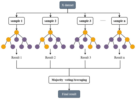
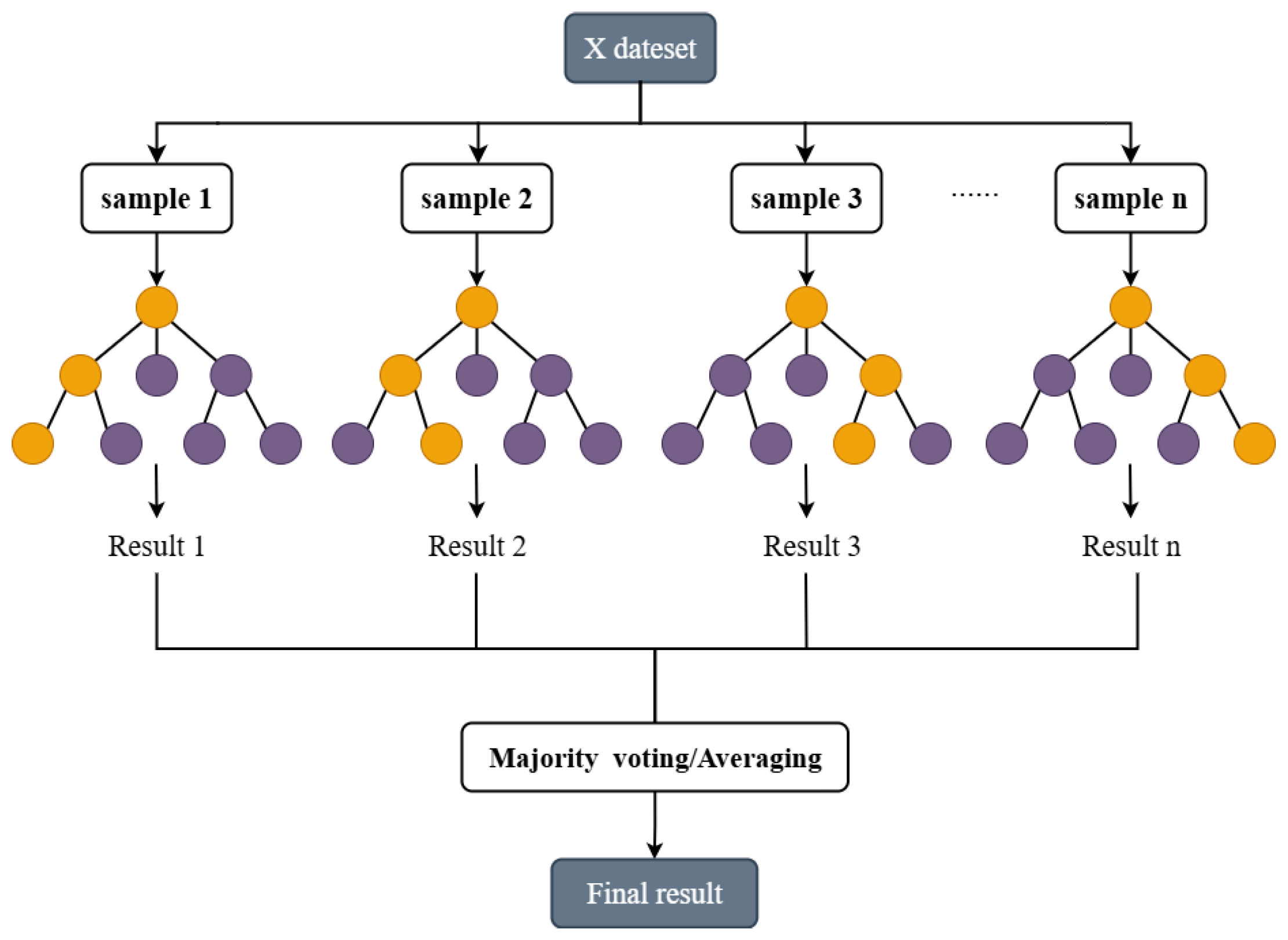
RF [43] is an ensemble learning algorithm based on Bagging that enhances model generalization by constructing multiple decision trees (DT) and combining their predictions. As shown in Figure 1, each DT employs bootstrap sampling to draw samples from the original dataset during training and randomly selects a subset of features for optimal node splitting.

Figure 1. Schematic diagram of the RF model (No explanation needed).

2.2.3. Artificial Neural Network

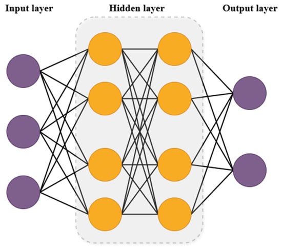
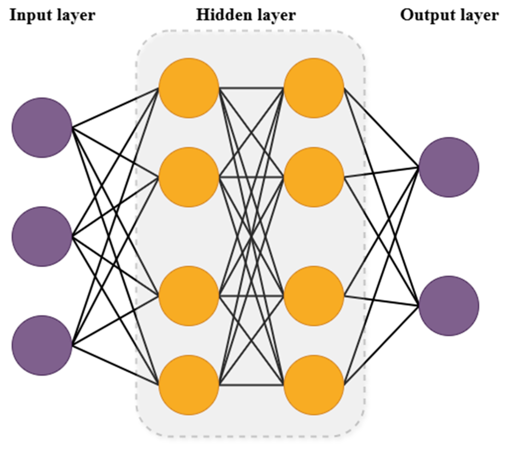
ANN [44] are machine learning models inspired by the structure of biological neurons. As shown in Figure 2, a neural network is formed by connecting multiple layers of neurons. Its basic structure includes an input layer, hidden layers, and an output layer [45,46]. The hidden layers can be stacked in multiple layers to form a deep neural network (DNN).

Figure 2. ANN model schematic diagram.

Common activation functions include Sigmoid, Tanh, ReLU, Softmax, and others. ANNs compute outputs through forward propagation, then update weights via backpropagation based on gradients calculated from the loss function.

2.2.4. Stacking

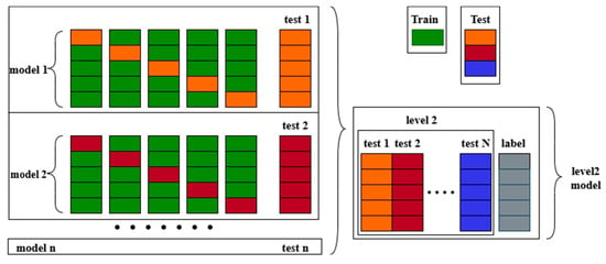
Stacking [47] is a hierarchical ensemble learning method. Its core concept involves enhancing prediction performance by feeding the outputs of base learners as new features into a meta-learner through a multi-level model architecture. Unlike parallel or serial ensemble methods such as Bagging and Boosting, Stacking employs homogeneous or heterogeneous base models and integrates them hierarchically via a meta-learner, effectively combining the strengths of different algorithms.

As shown in Figure 3, the basic structure of Stacking typically comprises two layers: The first layer consists of multiple base models. Each model independently learns from the training data and outputs its corresponding prediction results. The second layer introduces a meta-learner, which utilizes the prediction outputs from the first layer as new features. This meta-learner further learns the relationship between these predictions and the true labels, thereby optimizing the overall prediction performance.

Figure 3. Stacking algorithm schematic diagram.

This study selected RF, RR, and ANN as the base models, primarily due to their excellent empirical performance. As discussed in Section 4.1, these three algorithms stood out among the 13 machine learning models evaluated for oil production forecasting, emerging as the most accurate models. Furthermore, RF excels at nonlinear fitting and noise resistance; RR provides the necessary regularization constraints to mitigate multicollinearity among input features; and ANN offers powerful deep learning capabilities for complex pattern recognition. The heterogeneous stacked architecture not only overcomes the limitations of individual or homogeneous models but also fully leverages their highly complementary algorithmic strengths to achieve precise predictions.

2.3. Particle Swarm Optimization

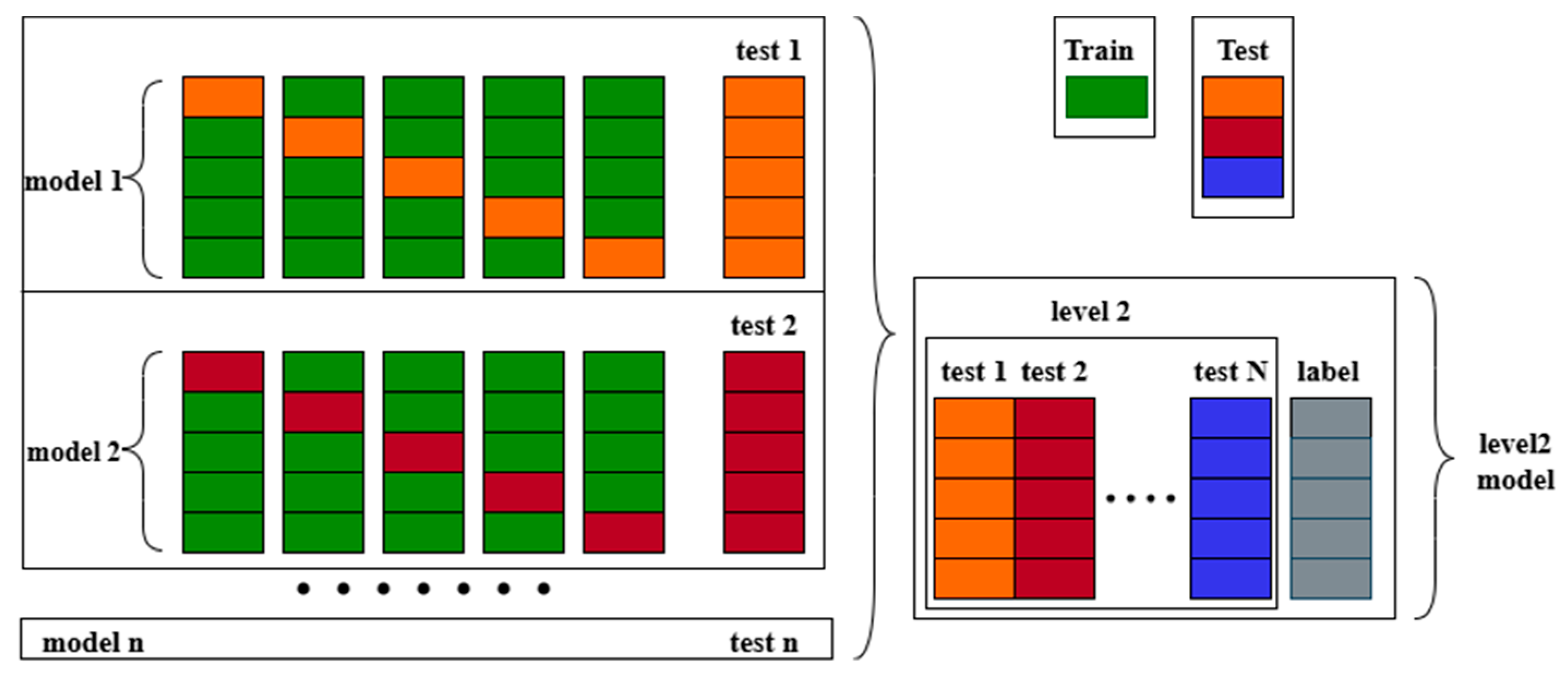
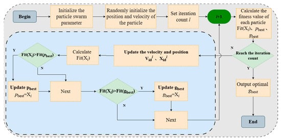
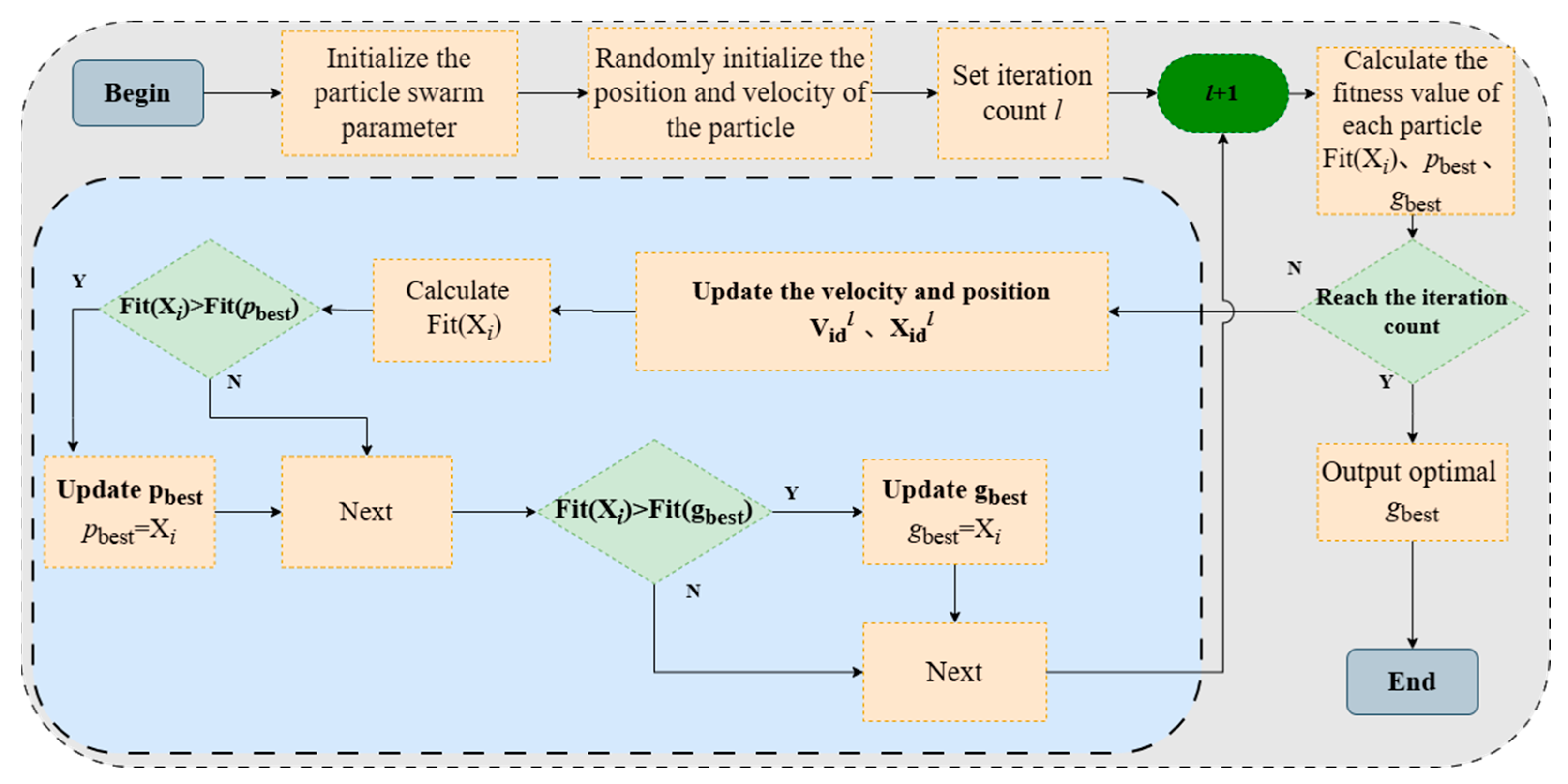
The PSO algorithm [48] is a global optimization algorithm based on swarm intelligence, as shown in Figure 4. The PSO algorithm initializes the particle swarm with random positions and velocities, and then iteratively updates the velocities and positions of each particle based on its personal best (p_best) and global best (g_best). In each iteration, the fitness values are evaluated, and p_best and g_best are updated accordingly. This process is repeated until the maximum number of iterations is reached, at which point g_best is output as the optimal solution.

Figure 4. PSO algorithm operational flow.

In the figure, l is the iteration count; ω represents the inertia weight; d is the dimension of the search space; i represents the i-th particle in the particle swarm; $v_{\mathit{id}}^l$ is the velocity of particle id at iteration l; $x_{\mathit{id}}^l$ is the position of particle id at iteration l.

2.4. Evaluation Indicators

The mean absolute error (MAE) is the average of the absolute values of the errors between the predicted values and the actual values in a dataset. Since the units of the predicted values match those of the actual observations, MAE better reflects the actual error in the predictions. MAE provides an absolute error metric; its value alone cannot directly indicate model quality and requires an evaluation through a comparison with other model results.

$$\begin{array}{c}MAE={\displaystyle \frac{1}{n}}{\displaystyle \sum _{i=1}^n}\left|y_i-{\widehat{y}}_i\right|\end{array}$$

(17)

Root Mean Square Error (RMSE) is the square root of the ratio of the sum of squares of deviations between predicted and actual values to the number of observations. It measures the average magnitude of deviation between predictions and actual values. This metric is commonly used to assess the accuracy of predictive models and is sensitive to outliers.

$$\begin{array}{c}RMSE=\sqrt{{\displaystyle \frac{1}{n}}{\displaystyle \sum _{i=1}^n}{\left(y_i-{\widehat{y}}_i\right)}^2}\end{array}$$

(18)

The coefficient of determination (R²) measures a regression model’s ability to explain the variability of the dependent variable. Its value indicates the proportion of variation in the dependent variable that can be explained by the independent variables through the regression relationship. R² ranges from 0 to 1, with values closer to 1 indicating better model fit. This metric essentially evaluates model performance by comparing the relative magnitude of prediction errors to the baseline error, using the mean of the dependent variable as the reference point.

$$\begin{array}{c}{R}^2=1-{\displaystyle \frac{{\sum }_i{\left(y_i-{\widehat{y}}_i\right)}^2}{{\sum }_i{\left(y_i-\stackrel{-}{y}\right)}^2}}\end{array}$$

(19)

2.5. Model Process

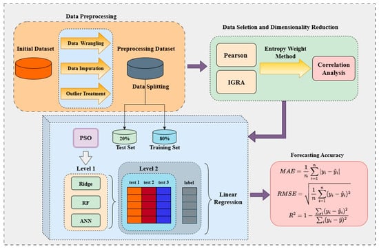
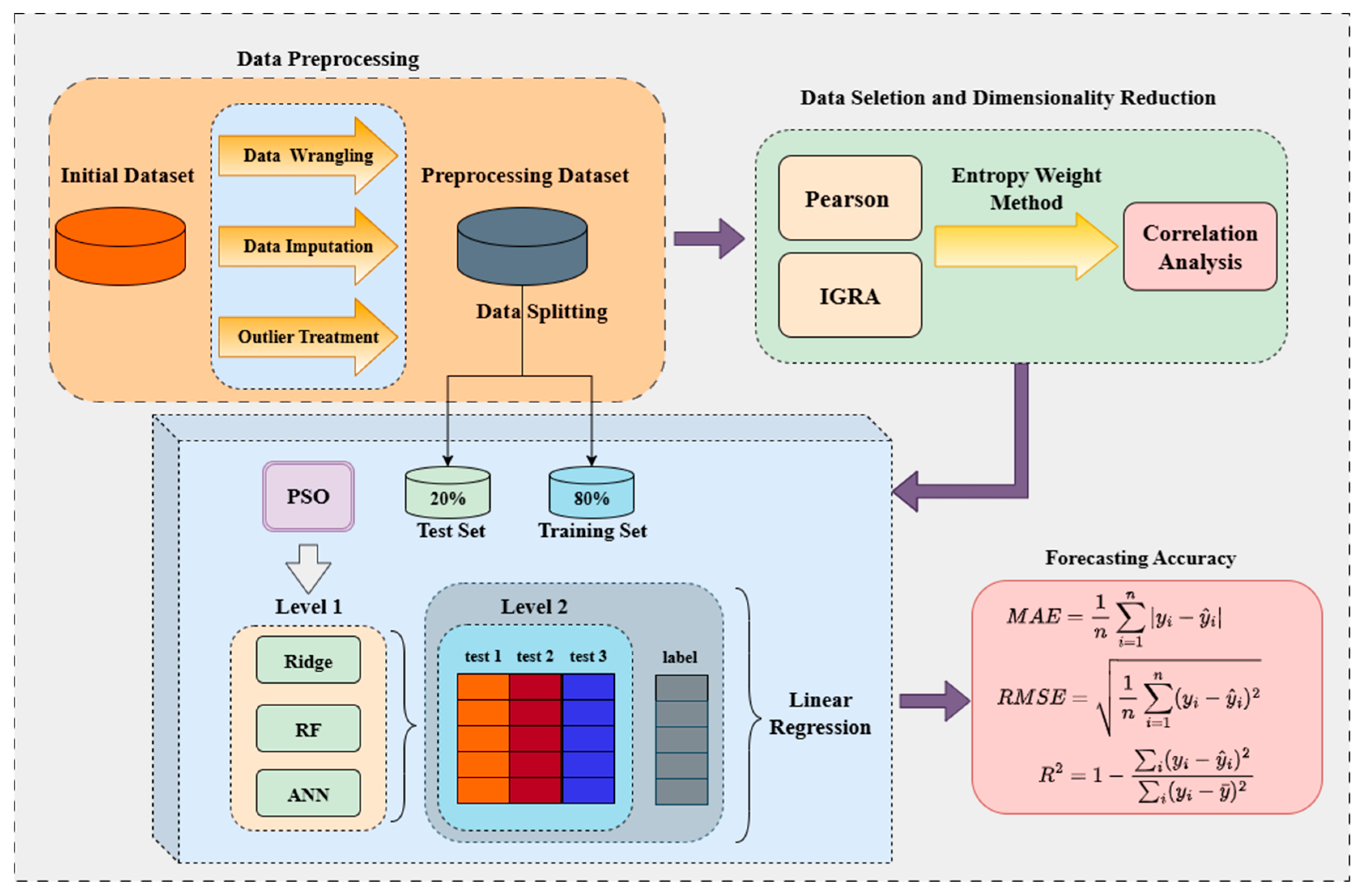
This study proposes a productivity forecasting framework based on an improved feature selection method and an ensemble learning model. The overall framework is illustrated in Figure 5, with the specific steps as follows:

Figure 5. Overall framework diagram of the integrated prediction model.

Step 1: Data Preprocessing.

Step 1.1: Handle missing values and outliers in the raw dataset.

Step 1.2: Standardize the processed dataset and partition it: 80% as a training set, 20% as a test set.

Step 2: Feature Selection

Step 2.1: Perform Pearson correlation analysis on the dataset; improve upon traditional GRA and conduct analysis.

Step 2.2: Perform weighted fusion of Pearson and IGRA for feature selection and dimensionality reduction.( The expression is correct.)

Step 3: Model Construction

Step 3.1: PSO optimization algorithm for hyperparameter search in RR, RF, and ANN models; optimized models serve as base models for the first layer of the Stacking model.

Step 3.2: Use the outputs from the first layer (test 1, test 2, test 3) as input features for the second layer, performing linear regression ensemble.

Step 4: Validate the established PSO + Stacking model by using evaluation metrics MAE, RMSE, and R².

All machine learning models, PSO optimization, and SHAP interpretability analyses in this study were implemented in Python 3.13.1 using the scikit-learn 1.0.2 and shap 0.40.0 libraries.

3. Data Analysis

To construct a reliable horizontal well productivity prediction model, this chapter systematically describes the data sources and characteristic parameters of the study block and details the data preprocessing workflow.

3.1. Data Preprocessing

This work focuses on tight oil reservoirs in the Ordos Basin, specifically the Chang 6 reservoir development system. Analysis was conducted on 320 wells from the selected block, incorporating geological parameters, engineering parameters, and production parameters as shown in Table 1.

Table 1. Characteristic parameters table.

Category	Parameter
Geological Parameters	Kelly Bushing Elevation (KBE), Target Formation (TF), Formation Temperature (FT), Total Depth (TD), Net Pay Thickness (NPT), True Vertical Depth (TVD), Bottom Hole Depth (BHD), Top Hole Depth (THD), Reservoir Thickness (RT), Spontaneous Potential (SP), Gamma Ray (GR), Shale Content (Vsh), Porosity (PHI), Permeability (K), Oil Saturation (So)
Engineering Parameters	Fracturing Time (Ft), Operation Time (OT), Fracturing Stage Count (FSC), Fracturing Method (FM), Fracturing Fluid System (FFS), Maximum Pump Rate (Qmax), Average Pump Rate (Qavg), Total Proppant Volume (TPV), Pad Volume (Vpad), Slurry Volume (Vslurry), Flush Volume (Vflush), Total Clean Fluid Volume (TCFV), Sand Ratio (SR), Minimum Treating Pressure (Ptreat/min), Maximum Treating Pressure (Ptreat/max), Average Treating Pressure (Ptreat/avg), Minimum Breakdown Pressure (Min BP), Maximum Breakdown Pressure (Max BP), Average Breakdown Pressure (Avg BP), Maximum Shut-in Pressure (Max SIP), Minimum Shut-in Pressure (Min SIP), Average Shut-in Pressure (Avg SIP), Completion Method (CM), Lateral Length (LL), Target Offset Distance (TOD), Wellbore Azimuth (WAZ), Entry Point (EP), Kick-off Point (KOP), Maximum Inclination (Max Inc)
Target parameters	Cumulative oil production (COP)

For the collected raw data, rigorous preprocessing was performed, including missing value imputation, outlier detection and handling, and data normalization. For missing values, given the limited number of missing data points, mean imputation was applied to supplement geological and engineering parameters. For feature variables with a missing rate exceeding 5%, they were directly discarded to avoid introducing excessive bias. For categorical variables such as FFS and FM, one-hot encoding is applied to prevent spurious order relationships between categories.

Outliers were removed using the 3σ principle, where data exceeding three times the standard deviation μ was considered an outlier, as expressed by the following formula:

$$\begin{array}{c}P(\left|x - \mu \right| > 3\sigma ) \le 0.003\end{array}$$

(20)

Additionally, to eliminate dimensional differences, the Min–max normalization method was applied to map all parameters to the [0, 1] range, enhancing data comparability. The expression is:

$$\begin{array}{c}{X}_{\mathrm{new}} = {\displaystyle \frac{X - \min (X)}{\max (X) - \min (X)}}\end{array}$$

(21)

Following the aforementioned preprocessing steps, the final dataset comprises 42 feature parameters from 250 wells, with significantly enhanced data quality, providing higher-quality data support for model training. Table 2 lists the count, mean, standard deviation, minimum, quartiles, and maximum for seven representative parameters. In the subsequent model training, the dataset of 250 oil wells was randomly split into two parts, with 80% forming the training set and 20% forming the test set, which was used to evaluate the model’s performance.

Table 2. The data information.

	NPT	RT	GR	Vsh	SR	FFS	COP
count	250	250	250	250	250	250	250
mean	11.02	770.25	82.03	25.36	12.15	8	2135.84
std	3.92	134.21	17.12	10.35	3.18	3	1487.32
min	4.00	354.70	64.38	14.28	7.19	1	31.89
25%	8.00	698.50	73.68	20.92	9.72	7	948.53
50%	11.00	772.50	79.88	23.85	11.78	7	1771.81
75%	13.00	832.00	85.3	26.3	14.55	11	2612.04
max	28.00	1168.00	224.96	150.36	18.66	17	6549.44

3.2. Correlation Analysis

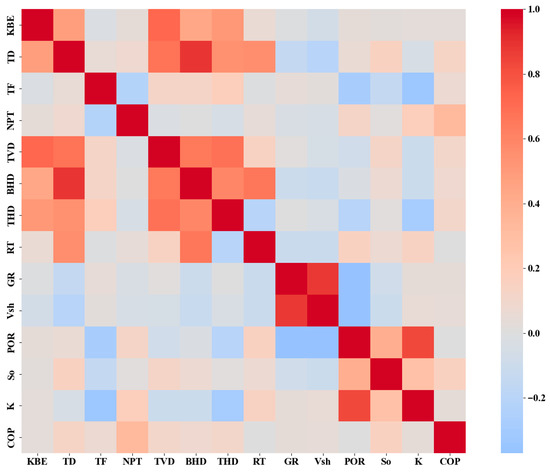
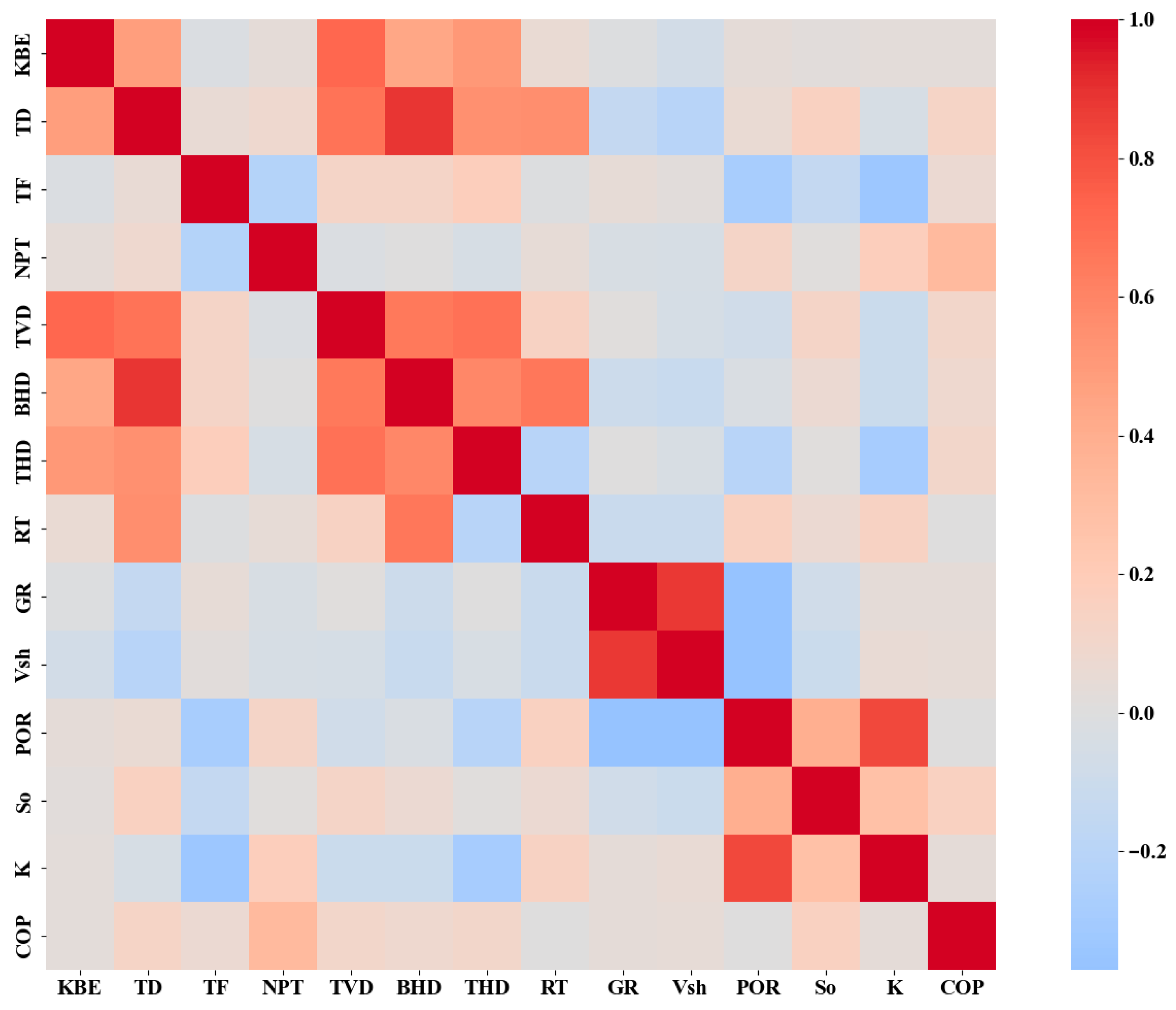
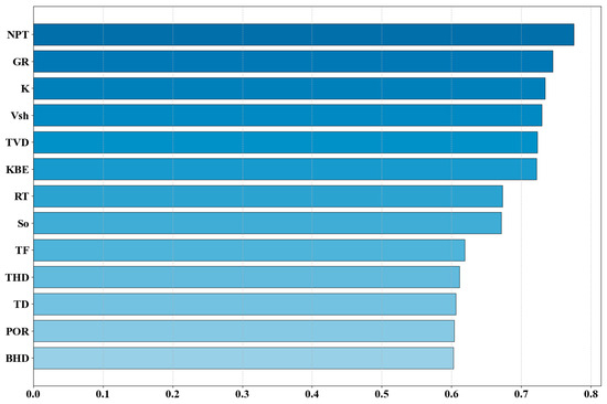
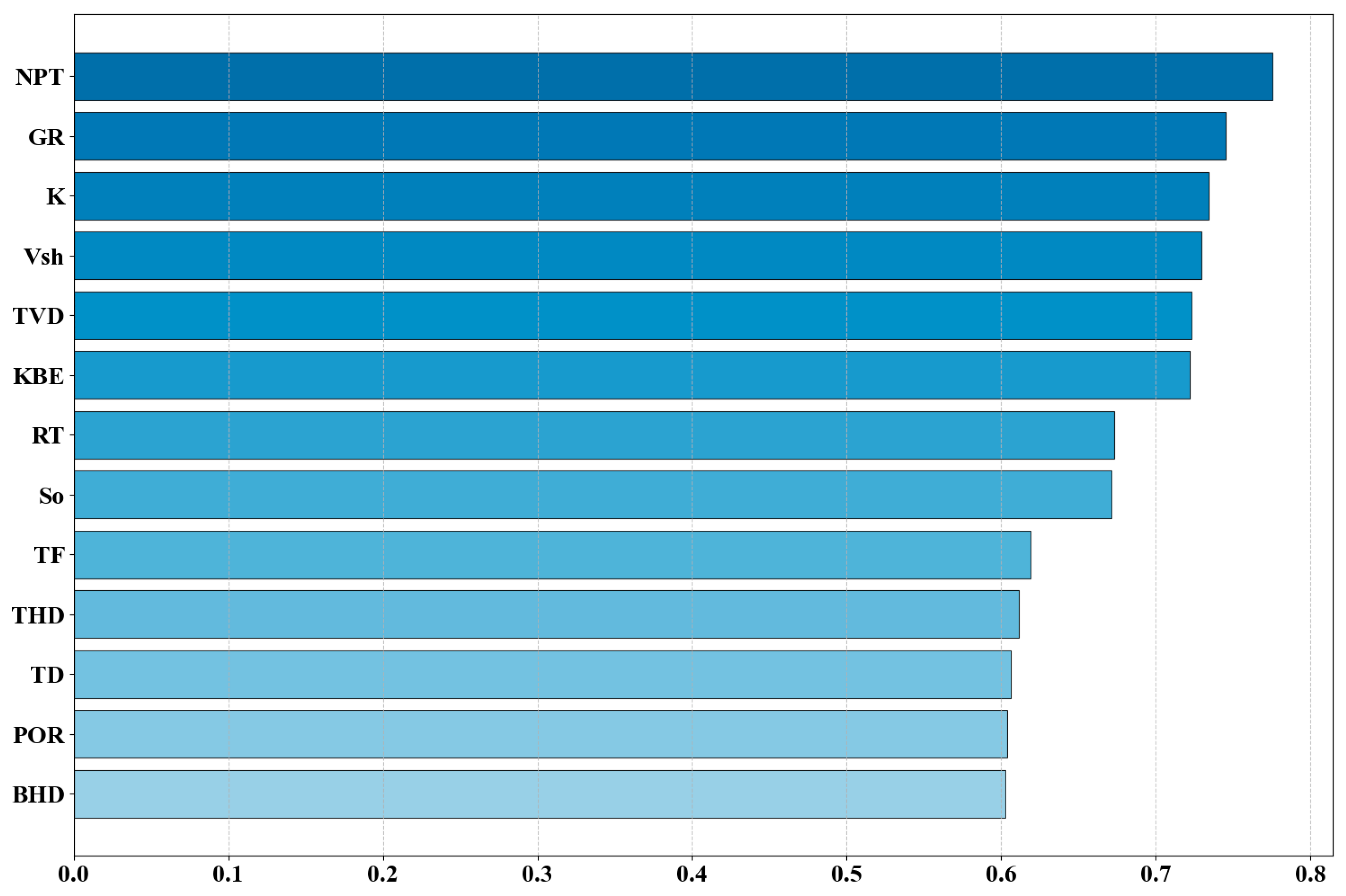
As shown in Figure 6 and Figure 7, both analytical methods consistently identify NPT as the most significant parameter influencing productivity. The Pearson correlation coefficient indicates a moderately strong positive correlation (r = 0.33), while IGRA assigns it the highest correlation value (η = 0.776). This indicates that better sand body development enhances reservoir connectivity and effective pore volume, thereby favoring hydrocarbon migration and production.

Figure 6. Geological parameters correlation heatmap.

Figure 7. Geological parameters IGRA degree ranking chart.

Pearson analysis reveals significant positive correlations between So (r = 0.15) and TF (r = 0.13) with productivity, reflecting the fundamental role of crude oil enrichment and deep reservoir endowment in production. IGRA further identified natural GR (η = 0.745) and K (η = 0.734) as highly correlated parameters from the perspective of systemic behavioral similarity, both closely related to lithology and pore structure. The divergence between the two methods’ results reflects their differing underlying mechanisms: Pearson correlation captures linear dependencies, while IGRA better captures trend synergies within complex nonlinear systems. This indicates that beyond saturation and burial depth, lithology and K are equally important physical parameters influencing productivity.

Notably, for POR, Pearson analysis revealed a very weak correlation with productivity (r = 0.03), and IGRA also indicated a relatively low association (η = 0.604). This consistent finding suggests POR is not a dominant factor in this study area, with its influence likely modulated by complex geological processes such as lithology, compaction, and diagenesis. Regarding inter-parameter relationships, Pearson analysis revealed strong correlations among well depth-related parameters (BHD, THD, TVD), reflecting their shared control by wellbore design and stratigraphic burial depth. Meanwhile, vertical depth maintained a high correlation (η = 0.723) in IGRA, indicating its continued significance in productivity regulation.

Both methods collectively indicate that correlations among most geological parameters are moderate or weak, suggesting relative independence in reservoir structure, physical properties, and fluid distribution.

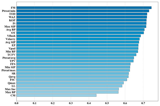
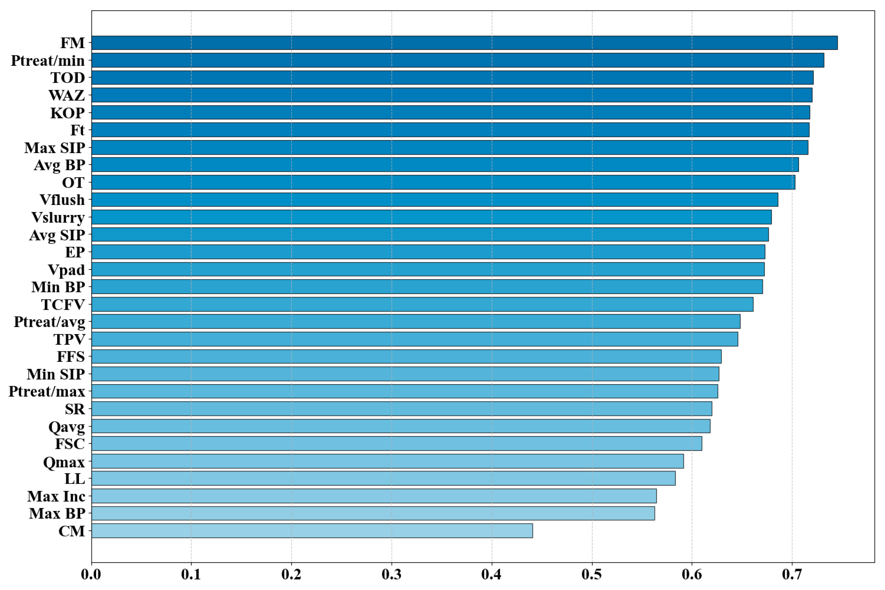
As shown in Figure 8 and Figure 9, among the engineering parameters, both methods jointly identified FM as the core control parameter (r = 0.31, η = 0.745). Its selection directly determines the morphology and flow-conducting capacity of the fracture network. V_fluid volume exhibits the strongest positive correlation (r = 0.46) in Pearson analysis and falls within the medium-to-high range of IGRA, jointly confirming its fundamental role in effectively fracturing formations and forming primary fractures.

Figure 8. Engineering parameters correlation heatmap.

Figure 9. Engineering parameters IGRA degree ranking chart.

Pearson analysis highlighted the importance of operational parameters like SR (r = 0.40), while IGRA further revealed the critical influence of integrated geotechnical parameters such as P_treat/min (η = 0.732) and TOD (η = 0.721). This indicates that formation initiation pressure and well-trajectory target point matching exert profound control over whether fractures can effectively communicate with hydrocarbon sources. Both methods consistently indicate that certain parameters have limited or even negative effects. FFS mismatched with reservoirs (r = −0.38), and intensity parameters like Q_max generally show low correlations. This suggests that blindly pursuing operational intensity rather than parameter compatibility may lead to energy dispersion or reservoir damage.

Two methods jointly identified the primary control parameter sequences affecting productivity: FM and V_fluid are the primary controlling factors; P_treat/min, TOD, and SR are key influencing parameters; while certain traditionally focused parameters, such as FFS and Q_max, are classified as inefficient or risk factors.

3.3. Comprehensive Weight Analysis

Section 3.2 separately evaluated the correlation or importance of each indicator in the dataset with the target variable using Pearson correlation and the IGRA method. While Pearson correlation effectively measures the linear correlation between variables, it has limited capability in capturing nonlinear relationships. Conversely, the IGRA method excels at handling complex, multifactor, and nonlinear associations, clearly quantifying the strength of connections between influencing factors and the research subject. However, it is relatively insensitive to fluctuations in the data itself. To avoid potential biases and limitations of a single method, accommodate both linear and nonlinear relationships, and enhance the scientific rigor and objectivity of evaluation results, this section employs the entropy weight method to conduct a fusion analysis of results from the two approaches. This method effectively combines the complementary information from two indicators. Both are dimensionless metrics, and after normalization via Equation (10), they form an evaluation matrix with consistent dimensions, satisfying the comparability requirements for data under information entropy theory.

Based on the original data and the above formula, the Pearson weight is approximately 68.4%, while the IGRA weight is approximately 31.6%. This ratio indicates that within the dataset, Pearson offers clear statistical interpretability and a foundation for hypothesis testing, making it more suitable as the primary basis for decision-making, while the IGRA weight serves as a supplement.

The comprehensive score table after weight fusion is shown in Table 3. It can be observed that parameters such as SR, V_pad, and V_flush rank highly in Pearson correlation and maintain their lead in the overall ranking. Meanwhile, parameters like NPT exhibit extremely high IGRA degrees; even if their Pearson correlation rankings are lower, they can still improve their overall ranking through the advantage of the IGRA degree.

Table 3. Ranking table of top 15 comprehensive scores after weighted integration.

Parameter	Pearson │ri│	IGRA	Overall Score
Vflush	0.449489 (3)	0.685753 (16)	0.524148 (1)
Vpad	0.451070 (2)	0.672240 (21)	0.520960 (2)
SR	0.457982 (1)	0.619647 (30)	0.509068 (3)
NPT	0.329860 (5)	0.775606 (1)	0.470716 (4)
FFS	0.379113 (4)	0.629370 (27)	0.458195 (5)
FM	0.312190 (7)	0.745191 (3)	0.449018 (6)
TPV	0.319902 (6)	0.645763 (26)	0.422874 (7)
Qavg	0.265948 (8)	0.618360 (32)	0.377310 (8)
OT	0.200569 (9)	0.702870 (15)	0.359296 (9)
TOD	0.141780 (15)	0.721304 (9)	0.324909 (10)
TCFV	0.164242 (11)	0.661311 (24)	0.321316 (11)
LL	0.199620 (10)	0.583248 (39)	0.320846 (12)
Avg SIP	0.153381 (13)	0.676212 (18)	0.318596 (13)
So	0.148998 (14)	0.671039 (22)	0.313963 (14)
Ptreat/avg	0.159393 (12)	0.648344 (25)	0.313901 (15)

3.4. Validation of Fusion Strategy Rationality

This section validates whether the weight allocation of the entropy weighting method is optimal by comparing multiple fusion strategies, such as EWM, Rank Aggregation (RA), Dempster–Shafer theory (D–S theory), and Equal Weight (EW), to ensure the rationality of its weighting.

Each fusion strategy produces a comprehensive feature ranking. The top 15 features from each strategy’s ranking form four distinct feature subsets. Using RF as the common baseline prediction model, the predictive performance of each feature subset on COP is evaluated. Performance comparisons are shown in Table 4:

Table 4. Performance comparison table of different fusion strategies.

Merger Strategy	RMSE	MAE	R2
EWM	325.1	282.3	0.835
RA	340.2	300.1	0.822
D-S	345.8	305.7	0.818
EW	341.5	298.7	0.821

Comprehensive comparison results demonstrate that EWM achieves the best performance in RMSE, MAE, and R². This highlights its advantage of objectively weighting information content, enabling a more effective extraction and integration of discriminative information from Pearson and IGRA measures. Consequently, it constructs a feature set with superior predictive capability. In contrast, other fusion strategies failed to outperform EWM due to insufficient information utilization, subjective assumptions, or neglecting the differential contributions between methods. Considering its optimal predictive performance, high computational efficiency, and fully objective implementation without requiring human-defined prior assumptions, the entropy weighting method is established as the most suitable strategy for integrating Pearson and IGRA information in this study.

4. Productivity Forecast Model

Based on the aforementioned correlation analysis results, this chapter constructs a PSO + Stacking ensemble learning model for productivity prediction by integrating multiple machine learning models. This is achieved by comparing the performance of datasets selected using two standalone methods and the fusion method. Finally, the SHAP framework is introduced for model interpretability analysis, revealing the influence mechanisms of various factors on productivity from both global and local perspectives.

4.1. Validation of Feature Selection Method Effectiveness

During the training and optimization of machine learning models, parameter selection exerts a decisive influence on predictive performance. To systematically explore the predictive capabilities of various models under different parameter combinations, this study employed filter methods [49] prior to model training. Specifically, the top 15 threshold, representing approximately 35% of the total features, was established to strictly isolate dominant factors and eliminate noise, while the top 25 threshold, accounting for approximately 60%, was chosen to balance dimensionality reduction with the retention of secondary features necessary for capturing synergistic interactions. Features were screened based on predefined rankings, resulting in the construction of six parameter comparison groups. By comparing the accuracy across each dataset, the optimal dataset was identified. Table 5 presents the six parameter combination comparison experiments:

Table 5. Description of parameter combination test cases.

Case	Illustration
1	IGRA correlation coefficient ηi (top 15)
2	IGRA correlation coefficient ηi (top 25)
3	Pearson correlation coefficient r (top 15)
4	Pearson correlation coefficient r (top 25)
5	Composite weight (top 15)
6	Composite weight (top 25)

To evaluate the effectiveness of the aforementioned six feature combinations, this study selected 13 machine learning algorithms as benchmark models for performance comparison. COP was designated as the target variable. The following thirteen models were employed: LR, RR, lasso regression (Lasso), SVR, DT, XGB, RF, gradient boosting decision tree (GBDT), adaptive gradient boosting (AdaBoost), ANN, polynomial regression (PR), light gradient boosting machine (LightGBM), and multi-layer perceptron (MLP) as benchmark models for performance comparison. The 250-well dataset was randomly split into an 80% training set and a 20% test set. Based on the normalized data, the performance of the models was evaluated using the three different model evaluation metrics described in Section 2.4 to select the optimal model and parameter combination. This study compared the models based on the evaluation metrics to identify the one with the best fit and lowest bias.

The performance metrics for each case are shown in Table 6. The hybrid weighting method demonstrated the best generalization performance (Case6, RMSE = 320.436, MAE = 289.397, R² = 0.844). This is because the hybrid method combines the strengths of both Pearson and IGRA, mitigating their individual shortcomings and providing a more comprehensive characterization of the feature space, thereby improving model accuracy. Regarding the number of features, the top 25 feature set consistently outperformed the top 15 set, indicating that increasing feature dimensions provides more comprehensive information and yields better feature synergy. Notably, Pearson outperformed IGRA when applied alone because Pearson better aligns with the data characteristics and underlying physical mechanisms, enabling clear identification of negative correlations. In predictive models, negative correlations are equally important as positive ones, as they provide counterintuitive predictive information.

Table 6. Performance comparison of different feature selection cases.

Name	Illustration	RMSE	MAE	R2
Case 1	IGRA correlation coefficient ηi (top 15)	461.429	439.221	0.750
Case 2	IGRA correlation coefficient ηi (top 25)	425.758	407.645	0.776
Case 3	Pearson correlation coefficient r (top 15)	385.974	349.877	0.812
Case 4	Pearson correlation coefficient r (top 25)	357.113	333.604	0.825
Case 5	Hybrid weight (top 15)	362.235	335.989	0.820
Case 6	Hybrid weight (top 25)	320.436	279.397	0.844

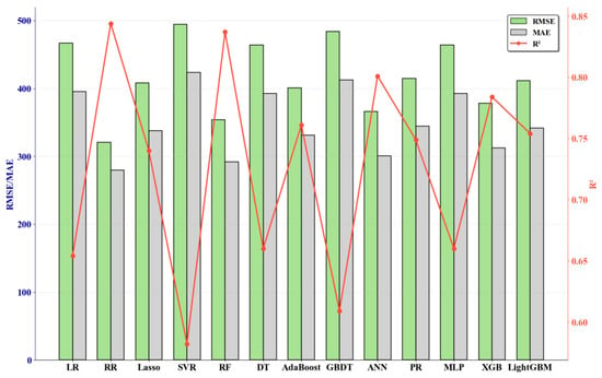
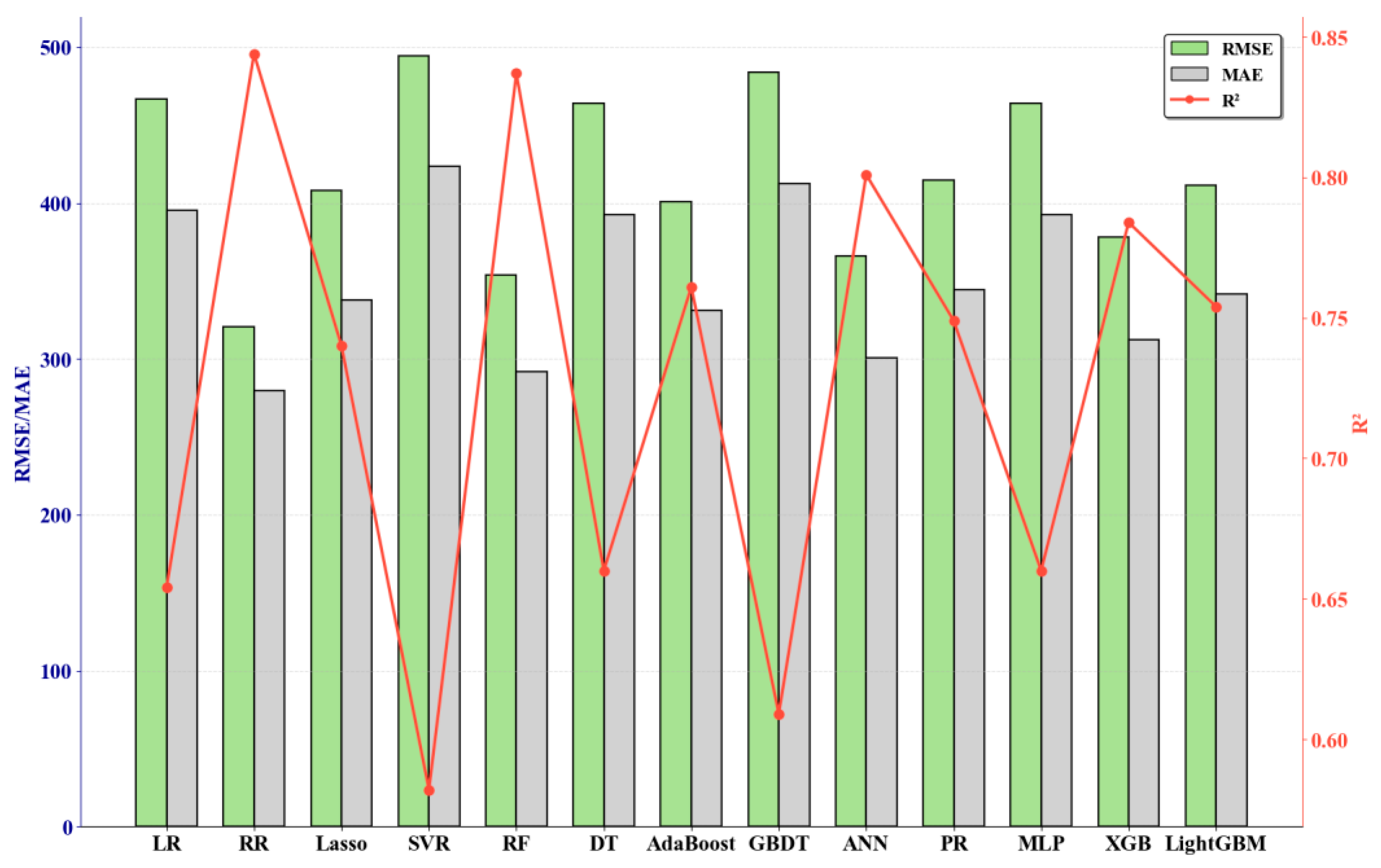
Figure 10 illustrates the prediction performance of different models for COP on the Case6 test set, along with their RMSE and MAE values. The figure indicates that RF (R² = 0.837), RR (R² = 0.844), and ANN (R² = 0.801) are the three most accurate models, demonstrating the highest precision in extracting and interpreting dataset features. Based on this, the feature set from Case6 is selected as the foundation for subsequent modeling. Furthermore, RF, RR, and ANN, which performed best on this feature set, will be chosen as the base learners for constructing the Stacking ensemble model.

Figure 10. Prediction performance of different models on the Case6 test set.

4.2. Verification of the Superiority of the Stacking + PSO Hybrid Approach

In this study, to achieve high-precision prediction of cumulative oil production from horizontal wells, a multi-layer regression model architecture was constructed using the stacking ensemble learning strategy. Specifically, three regression algorithms with the most outstanding performance and complementary characteristics were selected. As identified in Section 4.1, RF, RR, and ANN—three heterogeneous models—served as the first-layer base learners for the Stacking model. In the second layer, LR is employed to perform weighted fusion of the outputs from the base learners. The regression coefficients of this linear regression model clearly and quantitatively reflect the contribution weights of the three underlying base models to the final prediction results. Simultaneously, linear regression offers high computational efficiency and is less prone to overfitting. This ensures the deployability and generalization capability of the ensemble model in production environments, thereby constructing the Stacking regression prediction model. To quantitatively illustrate the specific contribution of each heterogeneous base model to the final prediction, the regression coefficients of the Level 2 linear meta-learner were extracted. The final assigned weights are 0.38 for RF, 0.42 for RR, and 0.20 for ANN. These coefficients demonstrate that the meta-learner effectively balances the robust nonlinear feature extraction capabilities of RF and ANN with the strict linear regularization constraints of RR, achieving an optimal algorithmic fusion.

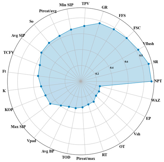
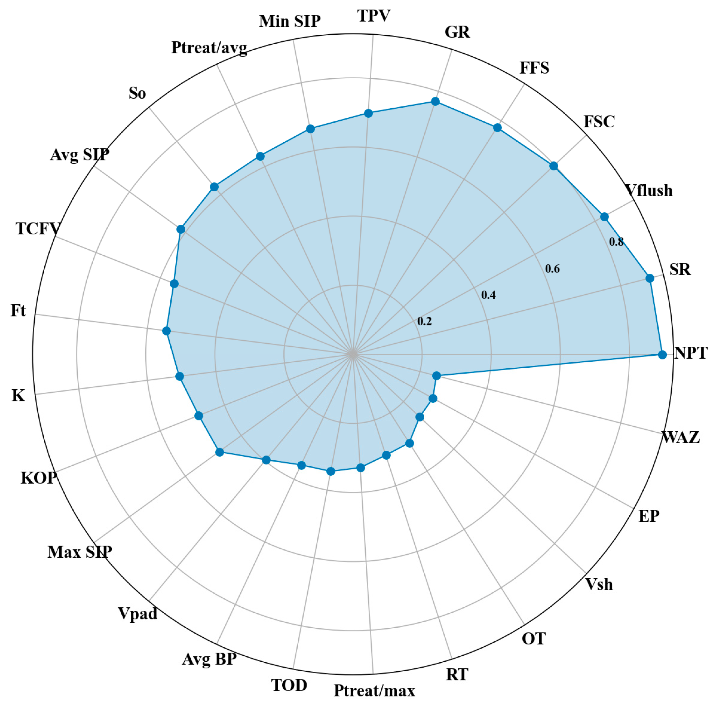
Figure 11 presents the parameter score map for the Stacking model. Consistent with the preliminary correlation analysis, the radar chart highlights that NPT and SR are the most dominant geological and engineering factors, respectively, with importance indices approaching 0.9. Other highly weighted parameters driving the model’s predictions include V_flush, FFS, GR, and So. These internal feature scores confirm that the ensemble model effectively prioritizes the primary physical and engineering drivers of tight oil productivity.

Figure 11. Radar chart of Stacking model scores.

To further enhance the predictive accuracy of the Stacking model and achieve global optimization of parameter combinations, this section employs the PSO algorithm for the collaborative optimization of hyperparameters in RF, Ridge, and ANN. PSO parameters are set as follows: 50 particles, maximum iterations of 100, acceleration coefficients c1 = c2 = 2, and an inertia weight ω that decreased linearly from 0.9 to 0.4 over the course of iterations. In each iteration, the objective is to maximize R², with candidate parameter sets evaluated using 5-fold cross-validation to determine fitness. The hyperparameter ranges for each base model are shown in Table 7. These ranges were determined based on a literature review and preliminary experiments to cover typical optimal intervals and avoid overfitting. The optimization process continued until fitness convergence (less than 10⁻⁴ improvement for 20 consecutive generations), ultimately selecting the parameter combination with the best cross-validation performance.

Table 7. Hyperparameter ranges for PSO optimization of base models.

Model	Hyperparameter	Optimization Range
RF	n_estimators	[50, 500]
	max_depth	[1, 20]
	min_samples_split	[2, 10]
	min_samples_leaf	[1, 10]
	max_features	[0.1, 0.9]
RR	ridge_alpha	[0.01, 100]
	ridge_fit_intercept	[0, 1]
ANN	hidden1	[20, 200]
	hidden2_ratio	[0.01, 0.3]
	Activation Function	[‘ReLU’, ‘Sigmoid’, ‘Tanh’, ‘Softmax’]
	alpha	[0.0001, 0.1]
	learning_rate	[0.001, 0.1]

These hyperparameter ranges were determined based on preliminary experiments and literature, designed to cover typical optimal intervals while mitigating the risk of overfitting or underfitting. By systematically adjusting these hyperparameters, the predictive accuracy and robustness of the models can be significantly enhanced.

After the rigorous PSO optimization process, the final optimal hyperparameters for the three base models were determined. These optimal values, which yielded the best cross-validation performance and were subsequently used to construct the final Stacking ensemble model, are detailed in Table 8.

Table 8. Optimal hyperparameters for the base model after PSO optimization.

Model	Hyperparameter	Optimization Range
RF	n_estimators	350
	max_depth	12
	min_samples_split	4
	min_samples_leaf	2
	max_features	0.6
RR	ridge_alpha	1.5
	ridge_fit_intercept	1
ANN	hidden1	128
	hidden2_ratio	0.12
	Activation Function	ReLU
	alpha	0.01
	learning_rate	0.005

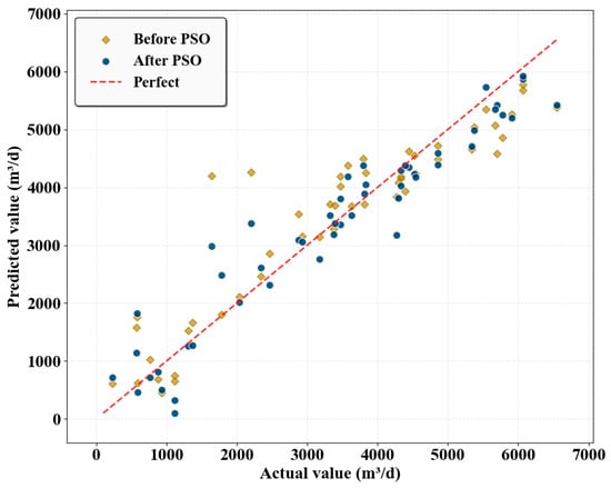
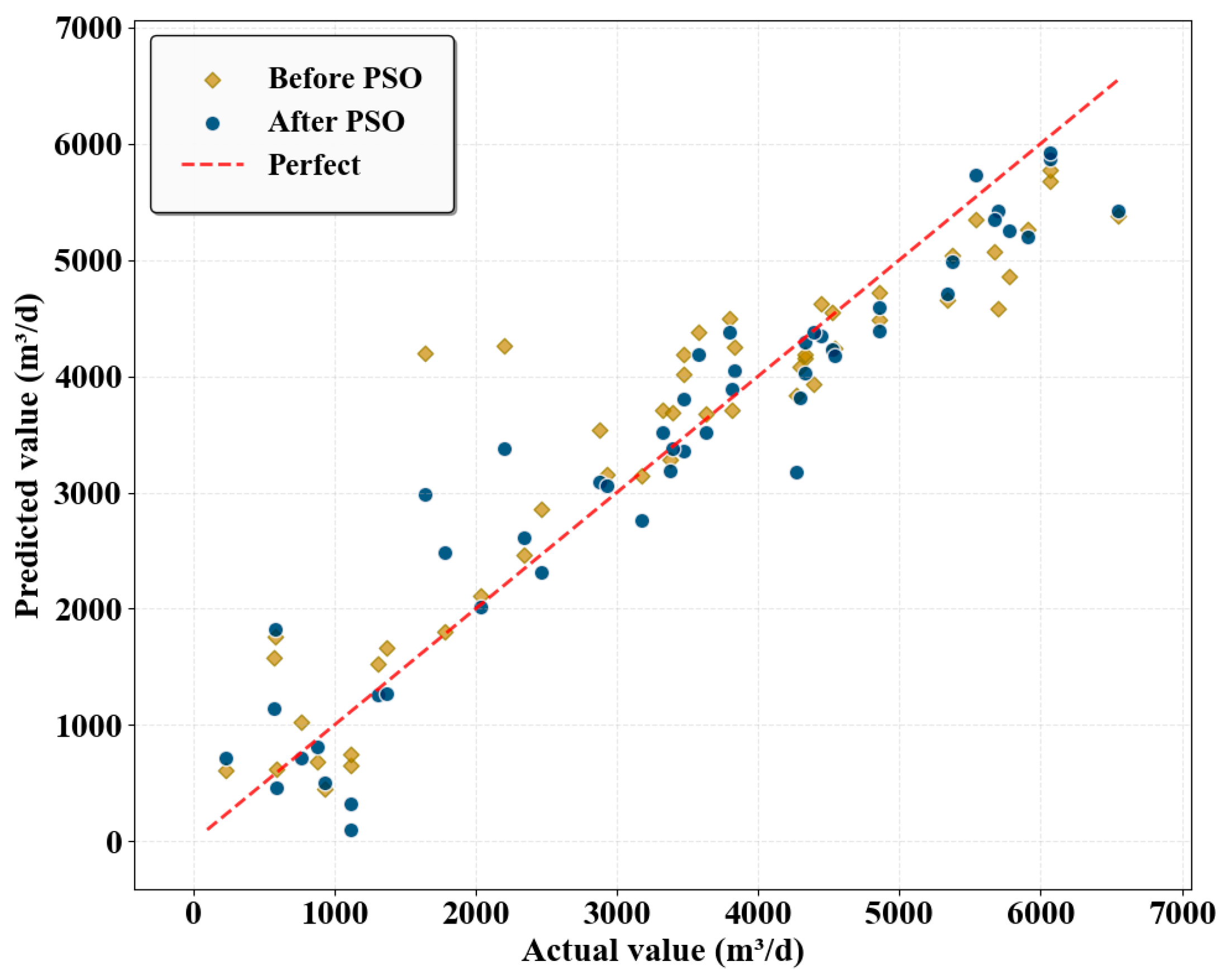
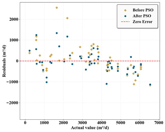
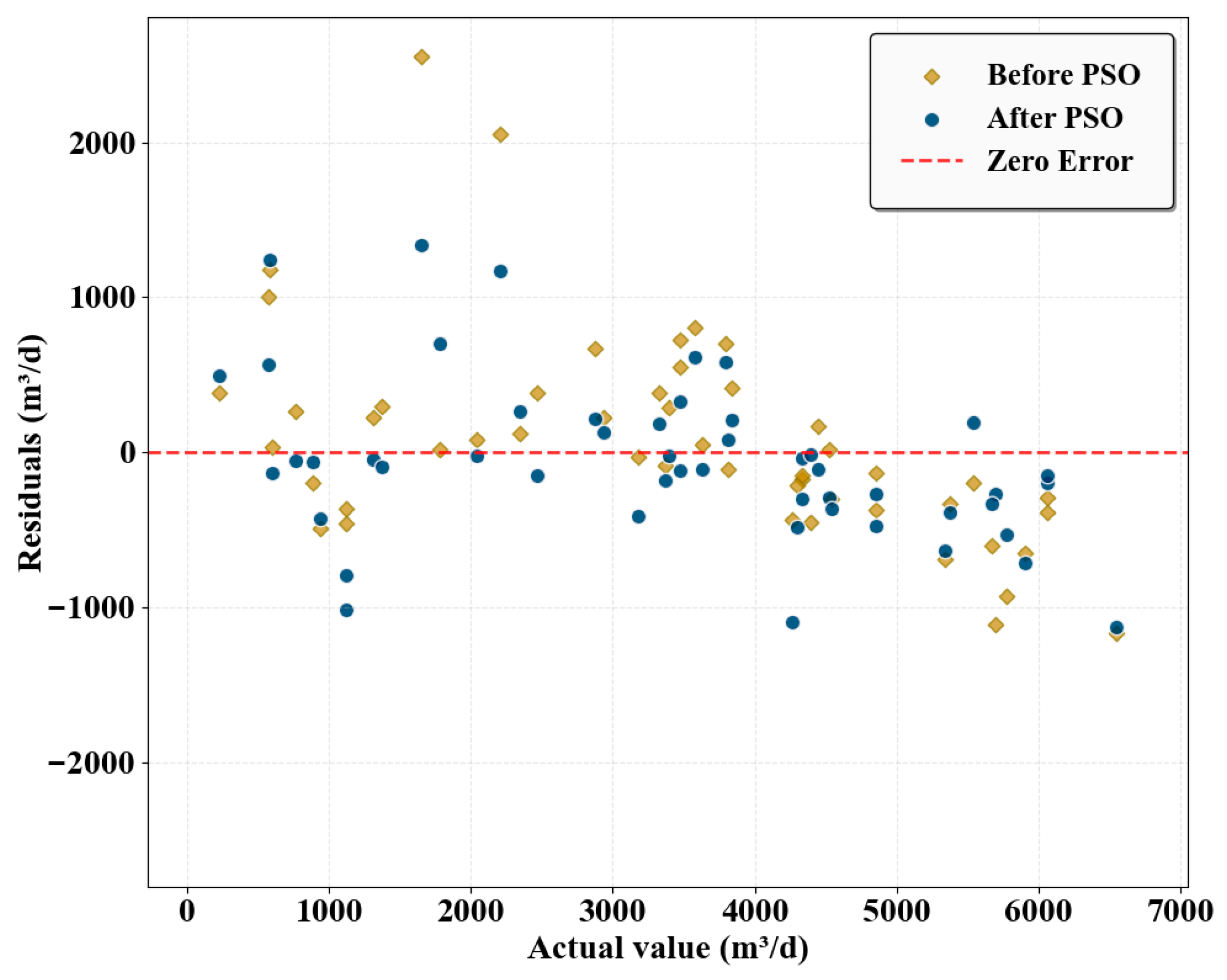
As shown in Figure 12, the scatter plot compares predicted and actual values before and after PSO optimization. Points closer to the diagonal indicate smaller errors. Before optimization, the Stacking model already showed reasonable fit, but the points were relatively dispersed. After PSO optimization, R² improved to 0.917, and the blue points clustered more tightly around the ideal line, confirming the algorithm’s effectiveness. Figure 13 presents the residual distributions. Before optimization, residuals fluctuated widely around the zero line, suggesting considerable model error. After PSO optimization, the residuals became significantly more concentrated, with reduced amplitude and dispersion around zero. This indicates improved error structure and prediction stability, consistent with the enhanced R² and tighter scatter observed in Figure 12.

Figure 12. Stacking model optimization before and after fitting diagram.

Figure 13. Stacking model optimization before and after residual distribution.

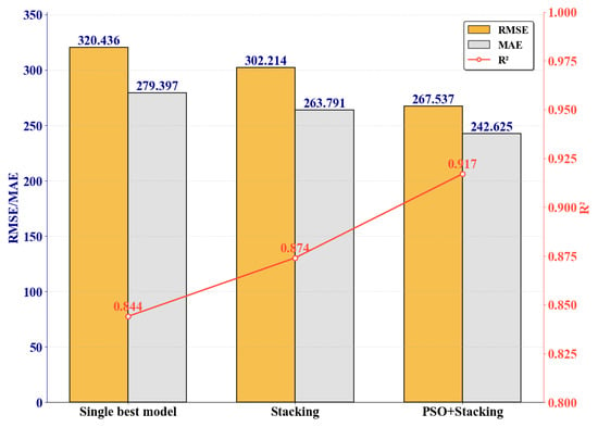
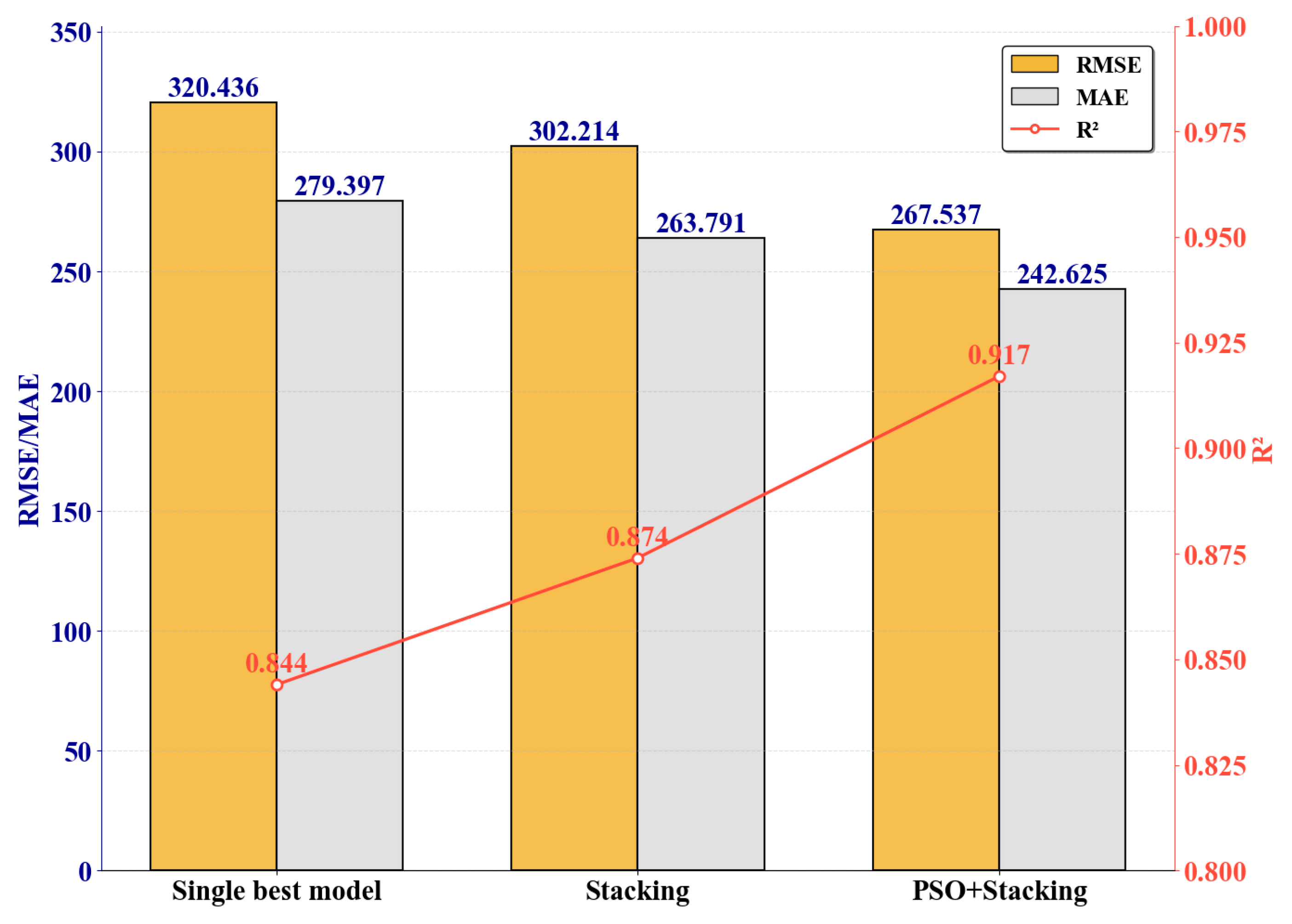
As shown in Figure 14, the optimized Stacking model demonstrates significant performance improvement after incorporating the PSO algorithm. The R² score increased from 0.874 to 0.917, indicating enhanced prediction accuracy and generalization capability. The RMSE decreased by 11.5%, and the MAE decreased by 8.0%, showing greater improvement in error metrics. Furthermore, compared to the best-performing single model (R² = 0.844), the PSO-Stacking model achieved even greater improvements: R² increased by approximately 8.7%, RMSE decreased by approximately 16.5%, and MAE decreased by approximately 13.2%. The consistent improvement across metrics indicates that the PSO algorithm effectively optimized the base model weights and meta-learner configuration, achieving an optimal balance between bias and variance. This result not only reflects the superiority of PSO in multi-model collaborative parameter tuning but also demonstrates that the selected base model combination exhibits high complementarity and effective information extraction capabilities.

Figure 14. Performance comparison before and after Stacking model optimization.

4.3. SHapley Additive exPlanations

To enhance model transparency, this section employs SHAP to provide global and well-specific explanations for the Stacking + PSO model. This approach reveals the specific influence mechanisms of each input feature on the model’s prediction outcomes, thereby improving the model’s interpretability and credibility in complex geological environments.

4.3.1. Global Feature Analysis

A global interpretability analysis was conducted on the optimized Stacking model. SHAP leverages the Shapley value concept from game theory to measure the average marginal contribution of each feature to the model output. A higher SHAP value indicates greater importance of the feature and a larger marginal contribution to the model output, thereby enabling quantitative analysis of the model’s internal mechanisms.

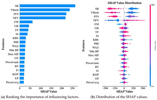
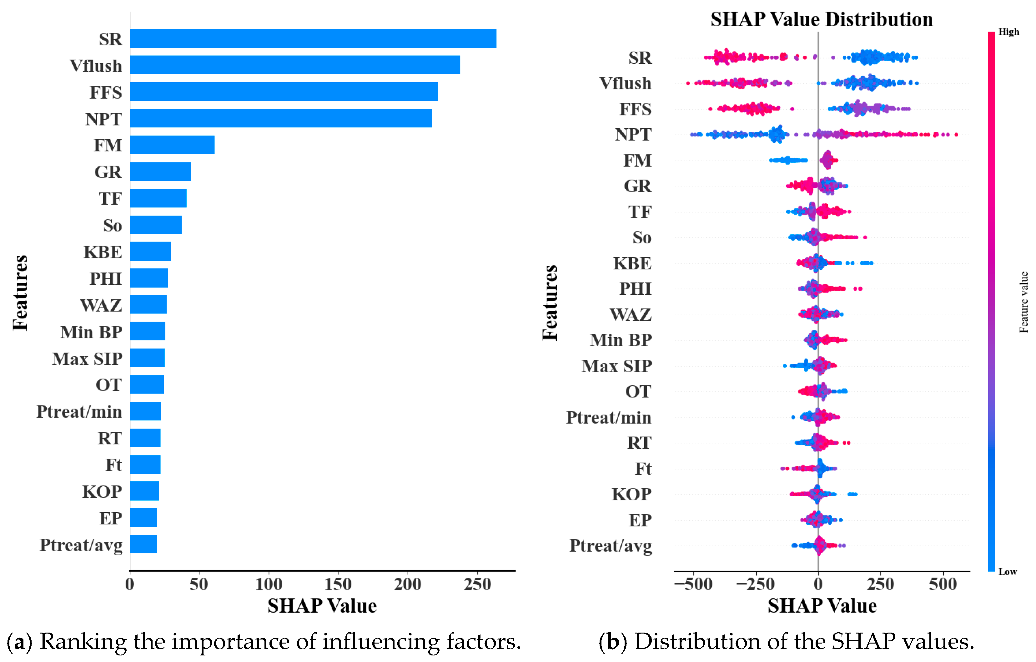
Figure 15a shows the SHAP feature importance ranking, which is based on the mean absolute SHAP value for each feature. It is evident that SR exhibits the most significant impact among all parameters, serving as the primary factor controlling horizontal well productivity. This indicates that fracture support strength and flow diversion capacity play a decisive role in the current reservoir stimulation effectiveness. V_flush, FFS, and NPT also have a substantial influence on the predictions. These variables collectively reflect the integrated contribution of formation modification to hydrocarbon productivity from perspectives, including reservoir properties, fracture connectivity, and fracturing fluid displacement efficiency.

Figure 15. Feature importance analysis results.

Figure 15b reveals the direction and magnitude of the impact of changes in feature values on the model’s predicted values. The figure indicates that SR, V_flush, and FFS exert a significant negative impact on oil production, with their high values (red points) corresponding to markedly negative SHAP values. Among these, SR exerts the most pronounced effect on oil production. This is likely because a high SR causes uneven injection water flow, increasing waterflooding difficulty and thereby reducing oil recovery efficiency. Additionally, an excessively high SR may trigger sand movement during production, leading to well blockages and diminished productivity. The negative effects of V_flush and FFS are also pronounced. Excessive displacement fluid and improper fracturing fluid formulations may overpressurize reservoirs, inhibiting natural hydrocarbon flow. Excessive displacement fluid volume can cause excessive fracturing within reservoirs, resulting in overly wide or uneven rock fractures that impair effective hydrocarbon flow pathways. Chemical components in FFS may react with reservoir rocks and fluids, causing sedimentation, blockages, or cementation phenomena that reduce reservoir recovery efficiency. Notably, NPT in the target layer exhibits a positive contribution, indicating that a greater reservoir thickness provides better enhanced volume conditions in the model, positively impacting production output. Other geological and engineering factors, such as FM, GR, TF, and So, exert minimal influence on COP and are therefore disregarded.

4.3.2. Single Well Analysis

To identify the primary factors limiting the productivity of low-yield wells and gain deeper insight into the mechanisms by which various influencing factors affect oil output, this study randomly selected one well for single-well interpretability analysis. This approach aims to avoid bias introduced by deliberately selecting high-yield wells, low-yield wells, or wells with optimal prediction accuracy, thereby revealing more universally and objectively how features within the model contribute to prediction outcomes. By analyzing the Shapley values of the randomly selected well, the decision logic of the model on typical samples can be reflected, facilitating the identification of key factors influencing oil production and their interaction mechanisms at the individual level.

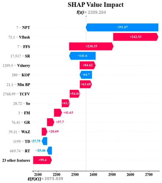
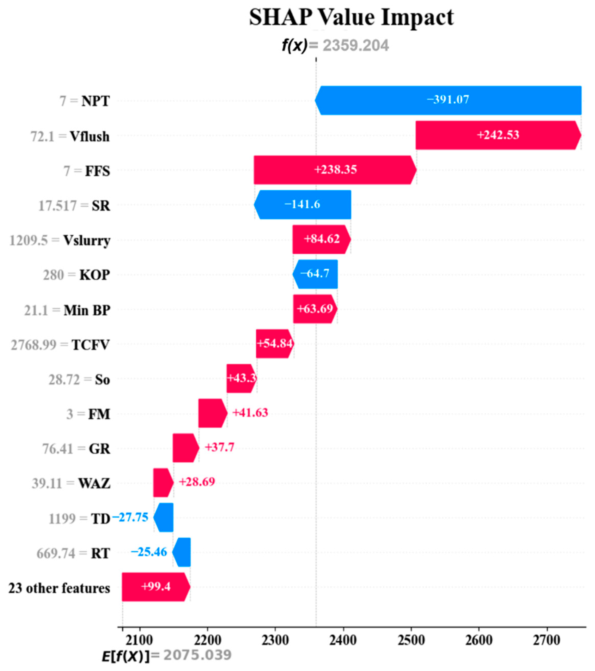
As shown in Figure 16, the SHAP local interpretability analysis indicates that the model predicts cumulative oil production for this well at 2359.204 m³/d. This prediction is higher than the model’s base value. This reflects a positive enhancement in production potential under the current parameter combination. The positive contribution primarily stems from engineering optimization parameters, with V_flush (+242.53) and FFS (+238.35) being the largest positive contributors. This indicates their critical role in proppant delivery and fracture expansion. V_slurry (+84.62), Min BP (+63.69), and TCFV (+54.84) further validate the rationality of fluid scale and construction pressure. Concurrently, geological and engineering parameters such as So, FM, GR, and WAZ also contributed synergistic gains.

Figure 16. Single well analysis chart (No explanation needed).

Negative impacts were primarily constrained by geological conditions and certain engineering parameters. NPT (−391.07) emerged as the most significant limiting factor; analysis suggests the current sand body thickness may restrict effective longitudinal fracture propagation, reducing fracturing energy utilization efficiency. SR (−141.6) similarly exhibited a significant negative effect, indicating that an elevated sand ratio under these conditions could increase near-wellbore friction or diminish proppant efficiency. Additionally, wellbore structural parameters such as KOP, TD, and RT exhibit minor negative effects, indicating their constraining influence on operational complexity and fracturing efficacy.

Comprehensive analysis indicates that the well’s production potential is significantly driven by engineering optimization. However, constrained by sand body thickness and sand ratio configuration, subsequent design plans require further adjustments in enhancing geologically driven drilling and optimizing sand ratios.

5. Discussion

This study developed a PSO-optimized Stacking ensemble learning model to post-fracturing productivity for horizontal tight oil wells. The results demonstrate that integrating a feature selection strategy based on comprehensive weight analysis with a heterogeneous ensemble learning framework significantly enhances prediction accuracy (R² > 0.91). Through SHAP interpretability analysis, this study not only identified the primary factors governing productivity but also provided direct data-driven insights for optimizing fracturing designs. The following discussion will focus on three key aspects: (1) the effectiveness of the methodology; (2) the complementarity between nonlinear mechanisms influenced by parameters and SHAP; (3) the engineering significance and limitations of the research.

Case 6 demonstrated the best performance, primarily due to its ingenious integration of Pearson’s linear statistical rigor with IGRA’s ability to capture trend changes, forming a more robust and comprehensive feature evaluation system. This stands in stark contrast to approaches based solely on Pearson analysis and IGRA (Cases 1–5), highlighting the superiority of the comprehensive weighting method proposed in this paper. The Stacking + PSO approach outperformed all single models because RF handles complex nonlinear interactions, RR provides linear stability, and ANN demonstrates powerful function approximation capabilities, while PSO optimization optimizes their combination. This demonstrates the immense potential of heterogeneous ensemble methods combined with intelligent optimization algorithms for solving complex industrial forecasting problems. Comparisons with existing literature reveal that the final performance metrics of this model surpass those of other methods reported in the literature (such as standalone XGB, SVR, or traditional numerical simulation), indicating a significant advantage in predictive accuracy.

SHAP analysis reveals that certain critical fracturing parameters, such as SR and V_flush, negatively impact production capacity in some wells. This appears to contradict their overall positive Pearson correlation and conventional engineering wisdom. This apparent discrepancy stems from the nonlinearity and context-dependent nature of parameter effects. SHAP values quantify the local marginal contribution of a feature within a specific well, while Pearson coefficients reflect the overall linear trend across the dataset. These two outcomes reveal the complexity of parameter effects from two distinct dimensions: global statistical trends and local conditional contributions. They are not mutually contradictory. In practice, exceeding the optimal operating windows for these parameters triggers severe geomechanical and hydrodynamic consequences. Under high closure stresses, excessive SR exacerbates proppant embedment and crushing, which degrades long-term fracture conductivity and risks near-wellbore screen-outs. Simultaneously, excessive V_flush causes over-displacement, leaving critical near-wellbore fractures unpropped and prone to premature closure after pumping stops. Consequently, negative SHAP values for these parameters primarily occur in wells where their values likely exceed the optimal range for the given well conditions, aligning with the concept of ‘over-fracturing.”

This study holds significant engineering guidance value, with specific recommendations including the following: ① Optimize pumping procedures: During construction, prioritize ensuring sufficient V_flush to guarantee effective proppant delivery, but keep it within the optimal local operating window to avoid over-displacement. Crucially, implement precise control of SR. Based on the block’s data, we recommend a safe and optimal SR adjustment range of 10% to 13%. Extreme SR designs exceeding 14.5% should be strictly avoided to prevent the severe geomechanical penalties identified by our SHAP analysis, such as proppant crushing and screen-outs. ② Implement differentiated fracturing strategies based on NPT: Given that NPT underpins productivity, fracturing designs must be dynamically matched to the specific sand body thickness. For thin target sand bodies, massive fluid injection should be restricted to avoid out-of-zone fracture height growth; instead, the design should focus on reducing perforation cluster spacing to enhance near-wellbore complexity. Conversely, for thick sand bodies, operators should aggressively increase TPV and V_pad to maximize the vertical and lateral expansion of the Stimulated Reservoir Volume. ③ Strengthen integrated geological-engineering decision-making: Prior to finalizing the fracturing design, it is recommended to input real-time logging-while-drilling data into our PSO-Stacking model for preliminary production potential estimation. This allows engineers to proactively adjust the aforementioned SR and fluid volumes to their optimal data-driven ranges for each specific stage.

This study has several limitations and future directions: all data originate from the same block; therefore, the model’s generalizability requires validation under other geological conditions. The model is static and does not account for dynamic production time data; certain engineering parameters, such as FFS, are categorical and difficult to quantify precisely. Future work will involve collecting multi-block data to develop cross-regional transferable prediction models and incorporating time series analysis to build dynamic production capacity prediction models. Additionally, we will explore more sophisticated feature fusion strategies, such as D–S evidence theory and nonlinear meta-learners.

6. Results

This study developed a PSO-optimized stacking ensemble learning model for accurately predicting the productivity of horizontal tight oil wells after fracturing. By integrating the strengths of multiple machine learning algorithms, the model significantly enhances prediction accuracy and generalization capabilities while providing clear, interpretable evidence for engineering decisions. Key findings are as follows:

(1)

Using datasets processed for missing values, outliers, and data standardization, Pearson correlation analysis and IGRA were employed to systematically evaluate the influence of geological parameters and fracturing engineering parameters on cumulative oil production. The results indicate that NPT (r = 0.33, η = 0.776) and FM (r = 0.31, η = 0.745) emerge as the two most critical production-controlling factors, exhibiting strong explanatory power for oil production and demonstrating typical characteristics of “easily controllable production.”

(2)

Based on the parameter combination comparison strategy (Case1–Case6), the model’s prediction accuracy and generalization capability significantly improved with optimized feature selection strategies. Ultimately, the feature combination constructed in Case6 (Composite weight (top 25)) performed best under ensemble models such as RF, RR, and ANN, achieving a maximum test set R² value of 0.844.

(3)

In the Stacking model, a multi-layer fusion prediction framework was constructed using RF, RR, and ANN as base models with LR as the meta-learner. PSO was introduced for hyperparameter tuning. This optimization resulted in a 4.9% improvement in R² for the Stacking model, while RMSE and MAE decreased by 11.5% and 8.0%, respectively.

(4)

SHAP analysis was applied to the Stacking model to enhance its interpretability and credibility. Based on Shapley values, parameter importance is ranked as follows: SR, V_flush, FFS, NPT, FM, GR, TF, So, etc. Single well feature analysis confirmed that parameter effects on oil production align with existing research, further validating the model’s reliability.

References

- Zhou, S.; Wang, J.; Liang, Y. Development of China’s natural gas industry during the 14th Five-Year Plan in the background of carbon neutrality. Nat. Gas Ind. 2021, 41, 171–182. [Google Scholar] [CrossRef]
- Zheng, L.; Wei, P.; Zhang, Z.; Nie, S.; Lou, X.; Cui, K.; Fu, Y. Joint exploration and development: A self-salvation road to sustainable development of unconventional oil and gas resources. Nat. Gas Ind. B 2017, 4, 477–490. [Google Scholar] [CrossRef] [Scilit]
- Qin, Y. Progress on geological research of deep coalbed methane in China. Acta Pet. Sin. 2023, 44, 1791. [Google Scholar] [CrossRef]
- Gao, D. Some research advances in well engineering technology for unconventional hydrocarbon. Nat. Gas Ind. B 2022, 9, 41–50. [Google Scholar] [CrossRef] [Scilit]
- Sun, L.; Fang, C.; Li, F.; Zhu, R.; He, D. Petroleum exploration and development practices of sedimentary basins in China and research progress of sedimentology. Pet. Explor. Dev. 2010, 37, 385–396. [Google Scholar] [CrossRef] [Scilit]
- Zou, C.; Yang, Z.; He, D.; Wei, Y.; Li, J.; Jia, A.; Chen, J.; Zhao, Q.; Li, Y.; Li, J.; et al. Theory, technology and prospects of conventional and unconventional natural gas. Pet. Explor. Dev. 2018, 45, 604–618. [Google Scholar] [CrossRef] [Scilit]
- Sun, L.; Zou, C.; Jia, A.; Wei, Y.; Zhu, R.; Wu, S.; Guo, Z. Development characteristics and orientation of tight oil and gas in China. Pet. Explor. Dev. 2019, 46, 1073–1087. [Google Scholar] [CrossRef] [Scilit]
- Zheng, Y.; Wang, H.; Tian, G.; Liu, M.; Li, G.; Kuru, E. Experimental investigation of proppant transport in hydraulically fractured wells using supercritical CO2. J. Pet. Sci. Eng. 2022, 217, 110907. [Google Scholar] [CrossRef] [Scilit]
- Zheng, Y.; Wang, H.; Wang, B. Effect of roughness characteristics of hydraulic fractures on the proppant transport using supercritical CO2. Geoenergy Sci. Eng. 2023, 227, 211908. [Google Scholar] [CrossRef] [Scilit]
- Long, T.; Li, G.; Wu, X.; Huang, Z.; Xie, Z.; Yang, R.; Song, X.; Tian, S.; Wang, H.; Hu, N. Vertical propagation behavior of hydraulic fracture guided by radial Borehole: Insight for horizontal well stimulation in multilayered reservoirs. Int. J. Min. Sci. Technol. 2025, 36, 229–249. [Google Scholar] [CrossRef] [Scilit]
- Yang, L.; Qingmin, Z.; Qi, L.; Zhaojie, X.; Xiaopeng, C.; Zupeng, L. Evaluation technology and practice of continental shale oil development in China. Pet. Explor. Dev. 2022, 49, 1098–1109. [Google Scholar] [CrossRef] [Scilit]
- Guo, J.; Ren, W.; Zeng, F.; Luo, Y.; Li, Y.; Du, X. Unconventional oil and gas well fracturing parameter intelligent optimization: Research progress and future development prospects. Pet. Drill. Tech. 2023, 51, 1–7. [Google Scholar] [CrossRef]
- Li, Z.; Gan, K.; Sun, S.; Wang, S. A new PM2. 5 concentration forecasting system based on AdaBoost-ensemble system with deep learning approach. J. Forecast. 2023, 42, 154–175. [Google Scholar] [CrossRef] [Scilit]
- Bai, W.-P.; Cheng, S.-Q.; Guo, X.-Y.; Wang, Y.; Guo, Q.; Tan, C.-D. Oilfield analogy and productivity prediction based on machine learning: Field cases in PL oilfield, China. Pet. Sci. 2024, 21, 2554–2570. [Google Scholar] [CrossRef] [Scilit]
- Fang, M.; Shi, H.; Li, H.; Liu, T. Application of machine learning for productivity prediction in tight gas reservoirs. Energies 2024, 17, 1916. [Google Scholar] [CrossRef] [Scilit]
- Chen, Y.; Xu, J.; Fu, L.; Chen, S. Review for SEPD model and YM-SEPD method, as well as establishment and application of PEPD model. Fault-Block Oil Gas Field 2020, 27, 766–769. [Google Scholar]
- Valkó, P.P.; Lee, W.J. A better way to forecast production from unconventional gas wells. In Proceedings of the SPE Annual Technical Conference and Exhibition, Florence, Italy, 19–22 September 2010; p. SPE–134231-MS. [Google Scholar] [CrossRef] [Scilit]
- Wang, Y.; Zhang, L.; Xu, J.; Bu, C.; Cao, Y. Empirical method for shale gas well production decline analysis optimization applied research. Petrochem. Ind. Appl. 2020, 39, 8–12. [Google Scholar]
- Sun, H. Exploration practice and cognitions of shale oil in Jiyang depression. China Pet. Explor. 2017, 22, 1–14. [Google Scholar] [CrossRef]
- Liu, W.; Zhang, X.; Sheng, S.; Wang, K.; Duan, Y.; Wei, M. Research on a new combination method of production decline analysis for tight oil: Cases study of Mahu tight reservoir. Pet. Reserv. Eval. Dev. 2021, 11, 911–916. [Google Scholar] [CrossRef]
- Xu, B.; Bai, Y.; Chen, L.; Li, Y.; Dong, Z. New cognition on shale oil and gas output successive decline pattern in Eagle Ford, US. Coal Geol. China 2021, 33, 15–19. [Google Scholar] [CrossRef]
- Yu, S.; Lee, W.J.; Miocevic, D.J.; Li, D.; Harris, S. Estimating proved reserves in tight/shale wells using the modified SEPD method. In Proceedings of the SPE Annual Technical Conference and Exhibition, New Orleans, LA, USA, 30 September–2 October 2013; p. D021S023R008. [Google Scholar] [CrossRef] [Scilit]
- Cai, J.; Peng, X.; Li, Q.; Zhan, T.; Wu, T.; Deng, Z.; Liu, W. Present situation and prospect of productivity evaluation of key marine carbonate gas reservoirs in Sichuan Basin. Fault-Block Oil Gas Field 2021, 28, 655–660. [Google Scholar] [CrossRef]
- Hu, J.; Zhang, C.; Rui, Z.; Yu, Y.; Chen, Z. Fractured horizontal well productivity prediction in tight oil reservoirs. J. Pet. Sci. Eng. 2017, 151, 159–168. [Google Scholar] [CrossRef] [Scilit]
- Sun, R.; Hu, J.; Zhang, Y.; Li, Z. A semi-analytical model for investigating the productivity of fractured horizontal wells in tight oil reservoirs with micro-fractures. J. Pet. Sci. Eng. 2020, 186, 106781. [Google Scholar] [CrossRef] [Scilit]
- MoradiDowlatabad, M.; Jamiolahmady, M. The performance evaluation and design optimisation of multiple fractured horizontal wells in tight reservoirs. J. Nat. Gas Sci. Eng. 2018, 49, 19–31. [Google Scholar] [CrossRef] [Scilit]
- Li, J.; Zhou, X.; Gayubov, A.; Shamil, S. Study on production performance characteristics of horizontal wells in low permeability and tight oil reservoirs. Energy 2023, 284, 129286. [Google Scholar] [CrossRef] [Scilit]
- Xu, J.; Yang, L.; Liu, Z.; Ding, Y.; Gao, R.; Wang, Z.; Mo, S. A new approach to embed complex fracture network in tight oil reservoir and well productivity analysis. Nat. Resour. Res. 2021, 30, 2575–2586. [Google Scholar] [CrossRef] [Scilit]
- Alharbi, O.Q.; Alarifi, S.A. Productivity index prediction for single-lateral and multilateral oil horizontal wells using machine learning techniques. ACS Omega 2023, 8, 7201–7210. [Google Scholar] [CrossRef] [Scilit]
- Zhu, R.; Li, N.; Liu, G.; Qu, F.; Long, C.; Wang, X.; Xiu, S.; Ling, F.; Liao, Q.; Li, G. Machine Learning-Driven Early Productivity Forecasting for Post-Fracturing Multilayered Wells. Water 2025, 17, 2804. [Google Scholar] [CrossRef] [Scilit]
- Anwar, M.; Radwan, T.; Salem, A.M.; Gad, R. Data-driven prediction of oil well productivity: Leveraging machine learning on pressure-test data. In Proceedings of the Offshore Mediterranean Conference and Exhibition, Ravenna, Italy, 8–10 April 2025; pp. OMC–2025-2657. [Google Scholar]
- Liu, W.; Chen, Z.; Hu, Y.; Xu, L. A systematic machine learning method for reservoir identification and production prediction. Pet. Sci. 2023, 20, 295–308. [Google Scholar] [CrossRef] [Scilit]
- Ning, Y.; Kazemi, H.; Tahmasebi, P. A comparative machine learning study for time series oil production forecasting: ARIMA, LSTM, and Prophet. Comput. Geosci. 2022, 164, 105126. [Google Scholar] [CrossRef] [Scilit]
- Lu, C.; Jiang, H.; Yang, J.; Wang, Z.; Zhang, M.; Li, J. Shale oil production prediction and fracturing optimization based on machine learning. J. Pet. Sci. Eng. 2022, 217, 110900. [Google Scholar] [CrossRef] [Scilit]
- Tong, S.; Wang, F.; Gao, H.; Zhu, W. A machine learning-based method for analyzing factors influencing production capacity and production forecasting in fractured tight oil reservoirs. Int. J. Hydrog. Energy 2024, 70, 136–145. [Google Scholar] [CrossRef] [Scilit]
- Ng, C.S.W.; Ghahfarokhi, A.J.; Amar, M.N. Well production forecast in Volve field: Application of rigorous machine learning techniques and metaheuristic algorithm. J. Pet. Sci. Eng. 2022, 208, 109468. [Google Scholar] [CrossRef] [Scilit]
- Pan, S.; Yang, B.; Wang, S.; Guo, Z.; Wang, L.; Liu, J.; Wu, S. Oil well production prediction based on CNN-LSTM model with self-attention mechanism. Energy 2023, 284, 128701. [Google Scholar] [CrossRef] [Scilit]
- Jebli, I.; Belouadha, F.-Z.; Kabbaj, M.I.; Tilioua, A. Prediction of solar energy guided by pearson correlation using machine learning. Energy 2021, 224, 120109. [Google Scholar] [CrossRef] [Scilit]
- Wang, X.; Wang, Y.; Tseng, Y.-Y.; Gao, Y.; Li, K.; Wang, M.-H.; Wu, J.; Lay, C.-H.; Huo, M. Integration of the grey relational analysis with machine learning for sucrose anaerobic hydrogen production prediction. Int. J. Hydrog. Energy 2024, 68, 388–397. [Google Scholar] [CrossRef] [Scilit]
- Wang, X.; Li, Y.; Qiao, Q.; Tavares, A.; Liang, Y. Water quality prediction based on machine learning and comprehensive weighting methods. Entropy 2023, 25, 1186. [Google Scholar] [CrossRef] [Scilit] [PubMed]
- Geraldo-Campos, L.A.; Soria, J.J.; Pando-Ezcurra, T. Machine Learning for credit risk in the Reactive Peru Program: A comparison of the Lasso and Ridge regression models. Economies 2022, 10, 188. [Google Scholar] [CrossRef] [Scilit]
- Hoerl, A.E.; Kennard, R.W. Ridge regression: Biased estimation for nonorthogonal problems. Technometrics 1970, 12, 55–67. [Google Scholar] [CrossRef]
- Salman, H.A.; Kalakech, A.; Steiti, A. Random forest algorithm overview. Babylon. J. Mach. Learn. 2024, 2024, 69–79. [Google Scholar] [CrossRef] [Scilit]
- Otchere, D.A.; Ganat, T.O.A.; Gholami, R.; Ridha, S. Application of supervised machine learning paradigms in the prediction of petroleum reservoir properties: Comparative analysis of ANN and SVM models. J. Pet. Sci. Eng. 2021, 200, 108182. [Google Scholar] [CrossRef] [Scilit]
- Ahmad, S.A.; Rafiq, S.K.; Hilmi, H.D.M.; Ahmed, H.U. Mathematical modeling techniques to predict the compressive strength of pervious concrete modified with waste glass powders. Asian J. Civ. Eng. 2024, 25, 773–785. [Google Scholar] [CrossRef] [Scilit]
- Ahmad, S.A.; Ahmed, H.U.; Rafiq, S.K.; Jafer, F.S.; Fqi, K.O. A comparative analysis of simulation approaches for predicting permeability and compressive strength in pervious concrete. Low-Carbon Mater. Green Constr. 2024, 2, 10. [Google Scholar] [CrossRef] [Scilit]
- Koopialipoor, M.; Asteris, P.G.; Mohammed, A.S.; Alexakis, D.E.; Mamou, A.; Armaghani, D.J. Introducing stacking machine learning approaches for the prediction of rock deformation. Transp. Geotech. 2022, 34, 100756. [Google Scholar] [CrossRef] [Scilit]
- Wang, D.; Tan, D.; Liu, L. Particle swarm optimization algorithm: An overview. Soft Comput. 2018, 22, 387–408. [Google Scholar] [CrossRef] [Scilit]
- Miao, J.; Niu, L. A survey on feature selection. Procedia Comput. Sci. 2016, 91, 919–926. [Google Scholar] [CrossRef] [Scilit]
Disclaimer/Publisher’s Note: The statements, opinions and data contained in all publications are solely those of the individual author(s) and contributor(s) and not of MDPI and/or the editor(s). MDPI and/or the editor(s) disclaim responsibility for any injury to people or property resulting from any ideas, methods, instructions or products referred to in the content. |
© 2026 by the authors. Licensee MDPI, Basel, Switzerland. This article is an open access article distributed under the terms and conditions of the Creative Commons Attribution (CC BY) license.