


Abstract
The distribution of gas–water two-phase flow in near-horizontal wells is influenced by factors such as wellbore inclination and phase flow rates. To explore these effects, a laboratory loop simulating downhole conditions was used to conduct experiments under varying inclinations and flow parameters. Flow patterns were classified based on visual observations and existing theory, and scatter plots were used to analyze flow regime boundaries. Three classification models were developed and compared. The proposed PNN–XGBoost framework integrates explicit second-order feature crossing with XGBoost-based importance selection prior to probabilistic neural network classification. Among the evaluated models, the PNN–XGBoost approach achieved the highest predictive performance. The model was further validated using 3D wellbore holdup imaging, confirming its robustness in flow pattern identification and its applicability to practical well logging interpretation.
1. Introduction
The flow patterns of gas–water two-phase flow in horizontal wellbores are more complex than those observed in oil–water systems, owing primarily to the significant differences in the physical properties of gas and water. Gas density and viscosity are much lower than those of water, resulting in faster and less stable gas-phase flow that is highly sensitive to gravity, flow rate, velocity, pressure, and temperature [1]. Such sensitivity causes the phase-interface distribution to fluctuate continuously during flow and leads to the formation of various patterns within the wellbore, namely, stratified flow, wavy flow, slug flow, and plug flow. These patterns not only transform into one another but are also closely related to wellbore inclination, completion type, and operating conditions [2,3,4].
To date, studies on gas–water two-phase flow patterns in horizontal wells have primarily employed two approaches [5,6,7]. The first uses computational fluid dynamics (CFD) software (ANSYS Fluent 2022 R2) for numerical simulation [8], while the second relies on physical experiments in simulated wellbores. CFD simulations offer low-cost modeling across diverse conditions but usually neglect instrumentation effects, resulting in discrepancies with actual downhole behavior. By contrast, physical experiments provide a more realistic flow environment that enables a deeper understanding of complex gas–water patterns, though they are costly and cannot cover all possible downhole scenarios. Nevertheless, many researchers have pursued experimental investigations. Mandhane et al. (1974) conducted horizontal gas–liquid pipeline experiments, produced pattern maps, and concluded that patterns are primarily governed by the superficial velocities of gas and liquid [9]. Liu et al. (2010) conducted gas–liquid two-phase flow experiments and found that flow patterns are influenced by total flow rate, fluid properties, and wellbore conditions [10]. Cui et al. (2021) performed logging experiments on simulated gas–water flow in horizontal wells, developed pattern maps, and determined that patterns are affected by total flow rate, water cut, and inclination angle [11]. Niu (2022) investigated two-phase flow at various inclination angles and reported that inclination angle exerts the greatest influence on gas–liquid two-phase flow patterns [12].
However, physical experiments, although providing authentic instrument-measured data, cannot encompass all downhole operating conditions due to the complexity of the subsurface environment. Consequently, an increasing number of researchers have begun to integrate artificial intelligence (AI) techniques to achieve more efficient and accurate flow pattern identification. For example, Liu et al. (2019) employed a backpropagation (BP) neural network, and Zhao et al. (2023) subsequently used a sparrow-search-algorithm-optimized BP (SSA-BP) network for this task [13,14]. While demonstrating AI’s strong modeling capability, BP networks suffer from slow convergence and a tendency to become trapped in local optima. Although powerful classifiers like XGBoost can perform well on large datasets, their performance on small, noisy experimental data—such as our 360-sample multiphase flow set—can be unstable. To address these limitations, this study proposes a novel PNN-XGBoost hybrid model, a two-stage architecture tailored for small-sample conditions. The core concept is to leverage the strengths of both methods while mitigating their individual weaknesses: XGBoost is employed not for final prediction, but as a robust front-end feature selector to identify and retain the most discriminative parameters from the noisy input set. This purified feature subset is then passed to a standard Probabilistic Neural Network (PNN)—which has been proven to outperform BP in classification tasks—for final, stable flow pattern classification. This approach effectively decouples feature robustness from classification stability. The inclusion of a PNN-BO variant (with Bayesian optimization) further demonstrates that the hybrid model’s superior generalizability on our data stems primarily from intelligent feature preprocessing, rather than merely from parameter tuning.
It is difficult to fully capture the complexity of downhole conditions solely through physical experiments and numerical simulations. In practical production logging [15], measurement tools deployed under high-temperature and high-pressure environments can acquire authentic downhole responses and generate fluid identification logs, such as density, dielectric water saturation, resistivity, or fiber-optic probe signals. These data can then be utilized for flow pattern identification through inversion techniques. Evidently, different flow regimes in the wellbore lead to distinct logging tool responses. Therefore, accurate recognition of flow patterns is essential for the inversion and interpretation of oil–water two-phase production profiles in horizontal wells. By integrating the real responses of logging tools with the theoretical insights provided by experiments and simulations, it becomes possible to analyze flow pattern characteristics more effectively and to select high-quality logging data under diverse operating conditions for comprehensive interpretation, thereby enhancing the accuracy of inversion and the reliability of interpretation results.
Therefore, this study integrates theoretical understanding derived from physical experiments with artificial intelligence techniques to improve flow-pattern prediction. Gas–water two-phase flow experiments were conducted in a full-scale downhole simulation loop under varying wellbore inclinations, flow rates, and water-cut conditions. These experiments generated a dataset that characterizes the relationships among flow patterns, superficial gas–water velocities, and wellbore inclination. Unlike small-scale wellbore models, numerical simulations, or multiphase flow databases, the full-scale experimental wellbore employed in this study more accurately replicates the actual downhole gas–water flow conditions and provides reliable flow parameters. Three deep learning-based neural network models were developed for flow-pattern prediction. Verification using three-dimensional wellbore holdup imaging demonstrates that the proposed PNN–XGBoost model achieves superior prediction accuracy compared with the other models. Furthermore, its superior recognition performance has been validated using field data within a three-dimensional spatial framework.
Furthermore, to improve the interpretability of the model’s predictions, this study introduces a three-dimensional visualisation approach that integrates spatial location, well depth and flow pattern prediction results. This method provides a clear and intuitive representation of wellbore flow behaviour and offers a new perspective for analysing flow regimes in multi-interval production wells.
In practical production logging, flow patterns are indeed a key intermediate variable for inferring phase behavior. However, direct downhole flow regime identification is often challenging. This study therefore addresses the forward prediction problem—estimating flow pattern from measurable parameters like phase velocities, pressure, and temperature. Establishing a reliable forward model is valuable for two reasons: (1) it enables flow regime diagnosis in settings where visual or imaging tools are not feasible (e.g., in permanent fiber-optic monitoring), and (2) it provides a physical constraint that can improve the well-posedness of subsequent inversion tasks, such as holdup or phase property estimation. Thus, the proposed model is designed to enable and enhance traditional interpretation workflows, not to replace them.
2. Materials and Methods
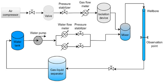
To approximate the downhole flow behavior in Chinese horizontal gas wells, a laboratory-scale flow loop was constructed. Under standard conditions (20 ± 2 °C, 101.325 kPa), air and tap water were used as the working media, with densities of 0.0012 and 0.9992 g/cm3, respectively. The main test section (Figure 1) consisted of a 16 m transparent acrylic wellbore with an internal diameter of 124 mm, connected to a gas–liquid separator, flow stabilizer, compressor, flow meters (accuracy ±8%), and a mixer. The optical fiber system was calibrated before each run to keep the measurement error within ±10%. After the flow rates were adjusted and held steady for about two minutes, data acquisition began. A high-speed camera positioned at the midpoint of the wellbore recorded each test for three minutes. If playback revealed any abnormal readings or unstable flow, the test point was repeated at least three times. The final recorded data were averaged over repeated measurements, thereby effectively reducing random measurement errors and improving the reliability of the experimental dataset.
Figure 1.
Schematic diagram of the experimental flow loop (measurement uncertainties: flowmeter ±8%; fiber-optic system ±10%).
At each test, fluid flow rates and water cuts were set on the control console. Fluid was then drawn from the water tank, pressurized, mixed, and injected into the simulated wellbore. Once the two-phase flow pattern stabilized, high-definition video recorded the gas–water flow patterns. After closing the gas inlet valve and waiting for water flow to stabilize, the pump was gradually ramped down, enabling fluid recirculation.
Given that gas wells with inclination angles exceeding 90° predominantly exhibit stratified and wavy flows [16], whose limited variation is difficult to distinguish instrumentally, this study focuses on uphill and horizontal flow patterns. Experiments were therefore conducted at four inclination angles, namely 83°, 85°, 88°, and 90°, with 83°, 85°, and 88° representing uphill flow and 90° representing horizontal flow.
In conventional gas well production, the volumetric flow rate of gas at the wellhead can increase by several hundred times when converted to downhole conditions due to temperature and pressure variations. Accordingly, the actual downhole gas production typically ranges from tens to several hundred cubic metres per day.
A major challenge in multiphase flow research is designing experiments that truly reflect real-world conditions. Previous studies have been useful, but they often have limitations in the range of conditions tested. For example, Zhao et al.’s (2023) study lacks data for the important conditions found in near-horizontal wells [14]. Niu (2022) et al.’s experiment, with just six conditions, doesn’t capture the complex interactions between different parameters [12]. Additionally, using small-diameter pipes in laboratory experiments, as in the studies by Syikilili, A.M. et al. (2021) and Li, L. (2019), raises questions about whether the results can be applied to actual wellbore conditions [17,18].
This study adopts a full-factorial experimental design covering 360 operating conditions, as summarized in Table 1. This design allows us to examine flow-pattern changes in a controlled way, especially under small variations in pipe inclination and water cut, which are common in near-horizontal wells. Before each test, the measurement system was calibrated to keep experimental uncertainty within ±10%. For unstable flow regimes, selected tests were repeated to confirm pattern consistency. These steps ensured that the final dataset was stable and reproducible, providing a sound basis for subsequent modeling.
Table 1.
Experimental scheme.
The operating ranges of gas superficial velocity, liquid superficial velocity, pressure, temperature, and pipe inclination were selected to reflect typical laboratory conditions for gas–water flow in near-horizontal wells, while remaining within the stable operating limits of the experimental loop. A full-factorial design was adopted to systematically explore all parameter combinations within these ranges, enabling a structured investigation of flow-pattern transitions under controlled conditions. Within this operating window, all flow regimes that physically occurred in the experiments were sampled repeatedly, resulting in a physically reliable and internally consistent dataset.
Although the dataset is robust from an experimental standpoint, its size is inherently limited by the cost and time requirements of multiphase flow experiments. We considered extending the dataset further; however, within the same operating range, doing so would have required a substantial increase in experimental runs while providing only limited additional flow-pattern information. For this reason, we prioritized constructing a well-controlled laboratory dataset that captures the essential flow-pattern transitions as clearly as possible under defined conditions.
As a consequence, the dataset reflects laboratory-scale behavior rather than the full complexity of field operations. The resulting models are therefore intended to support the analysis of flow-pattern trends and the evaluation of modeling strategies, rather than to serve as direct predictors for all industrial systems. This scope limitation is explicitly acknowledged and should be considered when interpreting the results and assessing their potential applicability to real production environments.
The experimental parameter ranges were designed to reflect realistic conditions and critical transitions in gas well production. The water cut (10–90%) covers the progression from the onset of liquid loading to dominant water flow. The specific lower limit of 10% approximates the critical carrying capacity for many gas wells, while 90% represents severe water production. Flow rates and inclinations were chosen based on an analysis of production data from several typical shale gas fields, ensuring the dataset encompasses the operational envelope for which the flow pattern prediction model is being developed.
3. Gas–Water Two-Phase Flow Patterns in Horizontal Wells
3.1. Theoretical Flow Patterns
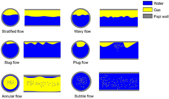
During gas–water two-phase flow, gravity acts perpendicular to the wellbore axis, causing the liquid phase to settle toward the lower portion of the pipe while the gas phase occupies the upper region. Moreover, the flow pattern is strongly influenced by well trajectory, total flow rate, and water cut, resulting in markedly different behaviors under varying operating conditions. Based on the seminal investigations of Mandhane et al. (1974) [9], Liu et al. (2010) [10], Cui et al. (2021) [11], and Niu (2022) [12] into gas–liquid two-phase flow in horizontal pipelines, six fundamental flow patterns can be identified, stratified flow, wavy flow, slug flow, plug flow, bubble flow, and annular flow, as shown in Figure 2.
Figure 2.
Schematic diagram of Gas–water two-phase flow patterns in horizontal wells.
Stratified flow occurs at low total volumetric flow rates. In this pattern, superficial velocities are low and phase interaction is minimal, resulting in a clearly defined, smooth interface between the gas and liquid phases. The lighter gas phase occupies the upper portion of the pipe, while the denser liquid phase settles below.
When water flow remains low with increasing gas flow, the slip between the phases intensifies the pattern transitions to wavy flow. Here, the gas–liquid interface begins to undulate, the distribution of gas and liquid becomes unsteady, and the flow exhibits pronounced oscillations.
As the overall flow rate and water cut further increase, the wavy interface rises to the top of the wellbore, forming slug flow. In this pattern, the gas phase in the upper section is broken into discrete slugs, producing an intermittent, plug-like flow characterized by alternating gas pockets and liquid segments.
Plug flow occurs when the water flow rate and water cut increase further, causing the lower-velocity gas phase to break into plug-like pockets within a continuous liquid column. Unlike slug flow, bubbles in plug flow assume ellipsoidal or irregular shapes, the flow becomes more intermittent, and gas pockets appear more dispersed throughout the liquid phase.
When water flow is very high and gas flow is low, the gas is broken into fine bubbles that are uniformly distributed within the liquid, thus producing bubble flow. Under gravity, these bubbles distribute irregularly in the horizontal pipe but tend to concentrate near the upper section of the pipe.
Annular flow emerges under conditions of high gas flow and low liquid flow. In this pattern, the high-velocity gas core transports liquid as a thin film along the pipe wall, while the pipe center is occupied by fast-moving gas laden with entrained droplets. This flow pattern is characterized by a continuous gas core and an annular liquid film, reflecting the strong entrainment capability of the gas phase.
3.2. Flow Patterns Observed in Our Experiments
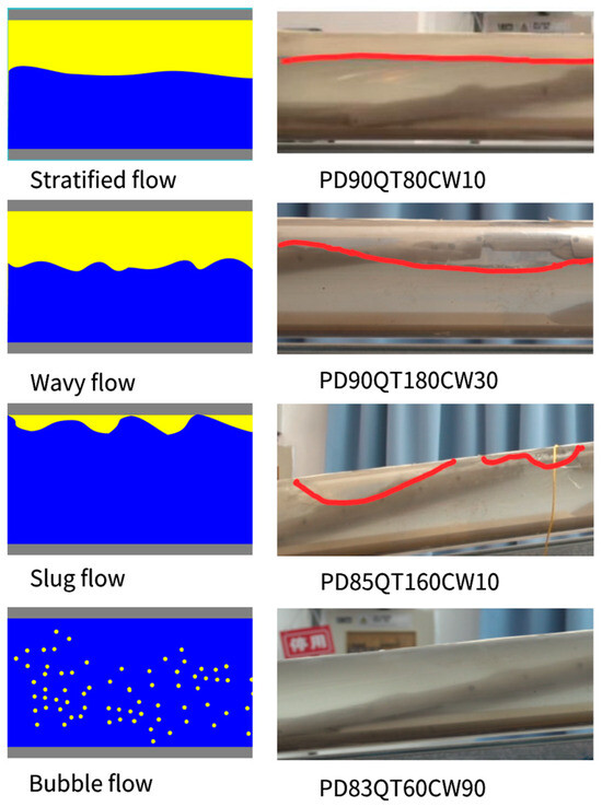
At each test point, flow patterns were initially determined through visual inspection of three-minute video recordings. For ambiguous transitional flows, such as the change from wavy to slug flow, measurements from fiber-optic and turbine flowmeters were systematically used as auxiliary criteria. For example, the transition from wavy to slug flow was defined by two concurrent conditions: (1) the appearance of periodic, large-amplitude peaks in the fiber-optic signal, and (2) visual confirmation from high-speed images that intermittent gas pockets occupied over 50% of the pipe diameter for a sustained period (>5 consecutive frames). This 50% blockage threshold is a commonly cited indicator for the formation of a distinct slug body. Such combined criteria provide an objective, repeatable basis for classification.
Based on the analysis of 360 experimental data points and referencing the classification scheme of Mandhane et al. [9], only four flow patterns—stratified, wavy, slug, and bubble flow—were observed under the current test conditions, primarily due to differences in wellbore geometry and fluid properties.
Although six fundamental flow patterns—stratified, wavy, slug, plug, bubble, and annular—are commonly recognized in horizontal gas–water flows, only four patterns were observed under our experimental conditions. This discrepancy primarily arises from the specific geometry of the laboratory wellbore, the selected inclination angles, and the physical properties of the working fluids (air and tap water). In particular, the combination of flow rates, water cuts, and pipe inclination used in this study did not meet the conditions necessary for the formation of plug flow and annular flow. Therefore, while the classical six-flow pattern framework provides a useful reference, the experimental dataset reflects the flow regimes that are physically realizable within the defined operating window. This also underscores the importance of calibrating classical flow regime standards to match specific operational and experimental conditions.
These results highlight the need to calibrate classical flow regime standards according to specific operational conditions and demonstrate the potential of multi-sensor data fusion to improve the reliability of complex flow pattern identification (As shown in Figure 3).
Figure 3.
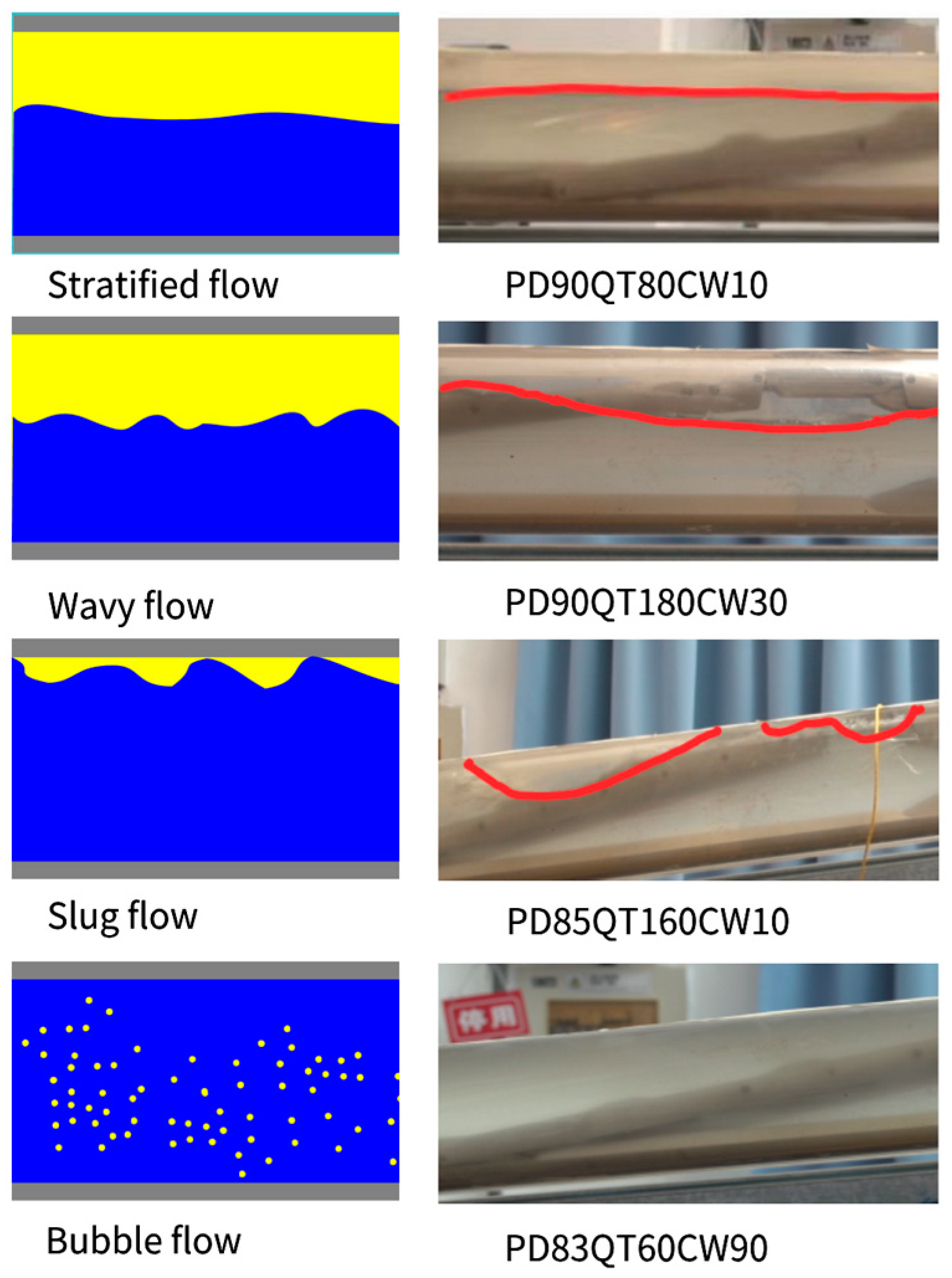
Flow patterns observed in our experiments, Please note that PD = inclination, QT = flow rate, and CW = water cut. The left column shows schematic representations, while the right column presents corresponding experimental images for comparison.
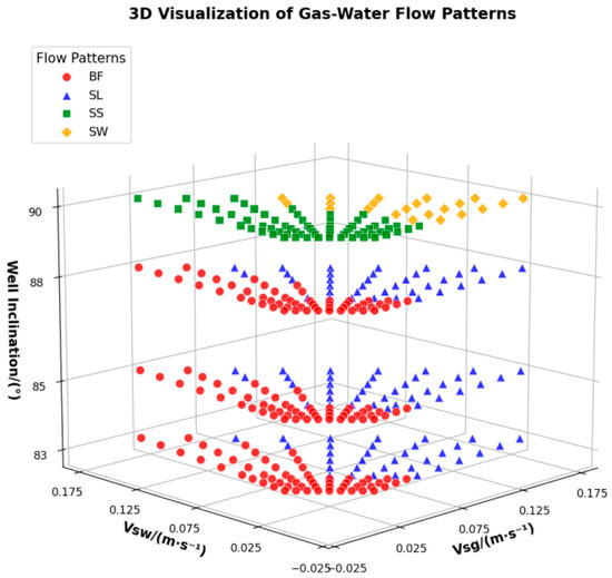
Based on the experimental data in prior studies [19,20], wellbore inclination and superficial velocities of phases are the principal factors controlling pattern transitions. Accordingly, these variables are presented as a scatter-matrix plot in Figure 4. The scatter-matrix visualization helps reveal the nonlinear coupling between inclination and phase velocities, justifying the use of a hybrid machine learning framework.
Figure 4.
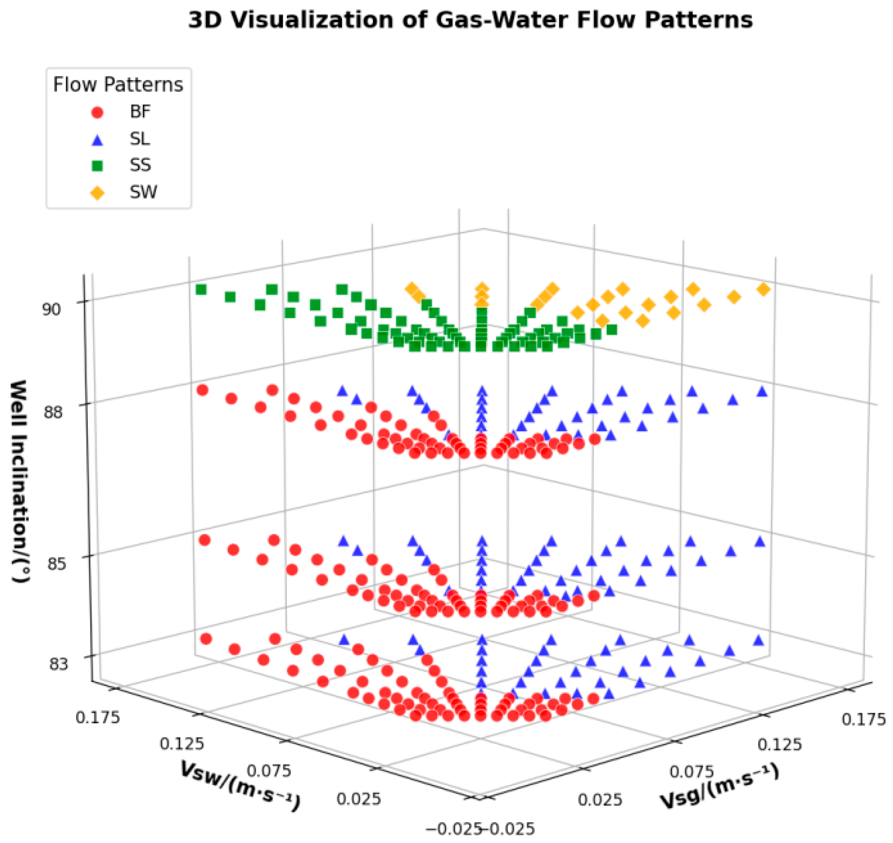
3D scatter plot showing the distribution of observed flow patterns in the experimental dataset. The plot highlights the influence of key variables, including wellbore inclination angle, superficial water velocity (Vsw), and superficial gas velocity (Vsg), on flow pattern behavior. The observed flow patterns are labeled as BF (bubble flow), SL (slug flow), SS (stratified flow), and SW (wavy flow). Each data point is labeled according to the observed flow pattern category obtained from experimental classification.
Flow patterns exhibit pronounced variation under different combinations of wellbore inclination and superficial velocity, indicating that pattern transitions follow consistent trends. These trends reflect the combined influence of inclination angle and superficial velocities of phases on fluid behavior within the wellbore and play a crucial role in the formation and evolution of flow patterns.
Pronounced differences in flow pattern transitions are observed between fully horizontal wellbores (inclination angle of 90°) and inclined wellbores (83°, 85°, and 88°). In the fully horizontal configuration, stratified and wavy flows predominate; and when superficial water velocity is held constant and superficial gas velocity is increased, the pattern shifts from stratified to wavy flow. Conversely, in inclined wellbores, slug and bubble flows dominate; under constant superficial water velocity, an incremental increase in superficial gas velocity drives a progressive transition from bubbly to slug flow.
The 3D Scatter plot in Figure 4 and the above analysis reveal relatively well-defined boundaries and trends among the observed patterns. In the complex, dynamic environment of multiphase flow, reliance on traditional analytical methods or manual classification cannot precisely delineate pattern boundaries or deliver reliable predictions. Conventional approaches usually fail to fully account for interactions among influencing variables, leading to imprecise pattern demarcation and suboptimal predictive performance. In contrast, deep-learning algorithms offer powerful data-processing and pattern-identification capabilities, enabling them to learn and exploit the intrinsic relationships among multiple parameters. By training on extensive experimental datasets, these algorithms can autonomously extract the governing rules of pattern transitions and determine the most reasonable boundary definitions.
4. Algorithmic Principles
Previous studies have applied backpropagation (BP) networks and their improved versions, such as SSA-BP, to flow pattern prediction. In this study, we tested their performance under small-sample conditions using experimental multiphase flow data. BP-based models have been reported to face practical difficulties in such situations, particularly due to their sensitivity to parameter initialization and susceptibility to overfitting when training data are limited [21]. These models typically require a relatively large amount of labeled data to reliably optimize a high number of trainable parameters, and collecting such data is often costly and time-consuming in multiphase flow experiments. In our preliminary tests, gradient-based training also showed slow or unstable convergence when the dataset was small and noisy.
To address these issues, we propose a hybrid PNN–XGBoost framework. The probabilistic neural network (PNN) uses kernel-based density estimation, which allows the model to capture nonlinear relationships between flow variables without iterative backpropagation, while reducing the number of parameters that require tuning. In the framework, an embedding layer converts discrete flow pattern information into a continuous form. This layer serves as a probabilistic feature mapping rather than a deep embedding structure commonly used in image or language models, thereby improving feature representation while maintaining model simplicity.
Next, XGBoost processes the probabilistic features produced by the PNN. XGBoost evaluates the importance of each physical variable and learns their interactions. Our input data are structured and low-dimensional. Under these conditions, the hybrid framework is more robust and less prone to overfitting when training samples are limited. While convolutional neural networks (CNNs) and long short-term memory networks (LSTMs) are primarily designed for image-based or sequential data, they are not specifically tailored for low-dimensional tabular datasets such as the flow pattern data considered here. For this reason, the PNN–XGBoost framework exhibits more stable training behavior and faster convergence in the present application. This observation is specific to the current experimental setting and does not imply a general superiority over other deep learning models.
4.1. PNN Model
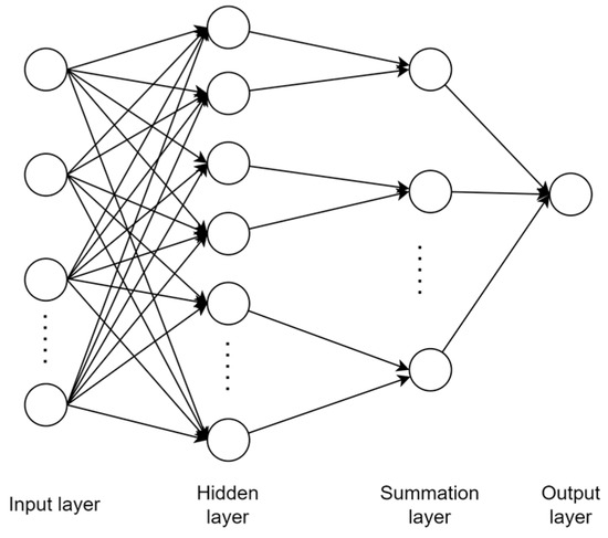
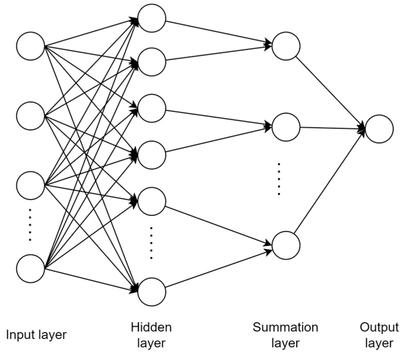
The Probabilistic Neural Network (PNN) is adopted for flow pattern prediction because it has a simple structure, fast training, and low expected error [22,23,24]. PNN classifies samples by comparing them to existing prototypes in the training data. The network has four layers, as shown in Figure 5:
Figure 5.
PNN architecture.
Input layer: receives raw features and applies any necessary preprocessing.
Hidden layer: measures the similarity between the input and each class prototype using a Gaussian kernel.
Summation layer: adds up the responses of all prototypes belonging to the same class.
Output layer: selects the class with the highest total response as the predicted flow pattern.
4.2. Bayesian Optimization
Bayesian optimization (BO) is used to automatically tune PNN hyperparameters, such as the smoothing parameter [25,26,27]. Instead of manually trying different values, BO suggests parameter settings based on past results to improve model performance. Integrating BO with PNN forms a PNN-BO framework that adapts to the dataset efficiently.
4.3. Extreme Gradient Boosting Algorithm
XGBoost is an ensemble method that builds multiple decision trees. Each tree corrects errors made by previous trees. In this study, XGBoost helps identify important features and capture complex interactions between variables. Its outputs are later combined with the PNN predictions to form a hybrid framework that benefits from both approaches [28,29,30].
4.4. PNN-XGBoost Hybrid Model
To tackle the data scarcity in gas–water flow pattern prediction, we designed a PNN–XGBoost framework with a feedback loop as its core mechanism. In this framework, XGBoost is employed not as an optimizer but as a feedback provider that guides feature selection and kernel parameter adjustment based on classification performance.
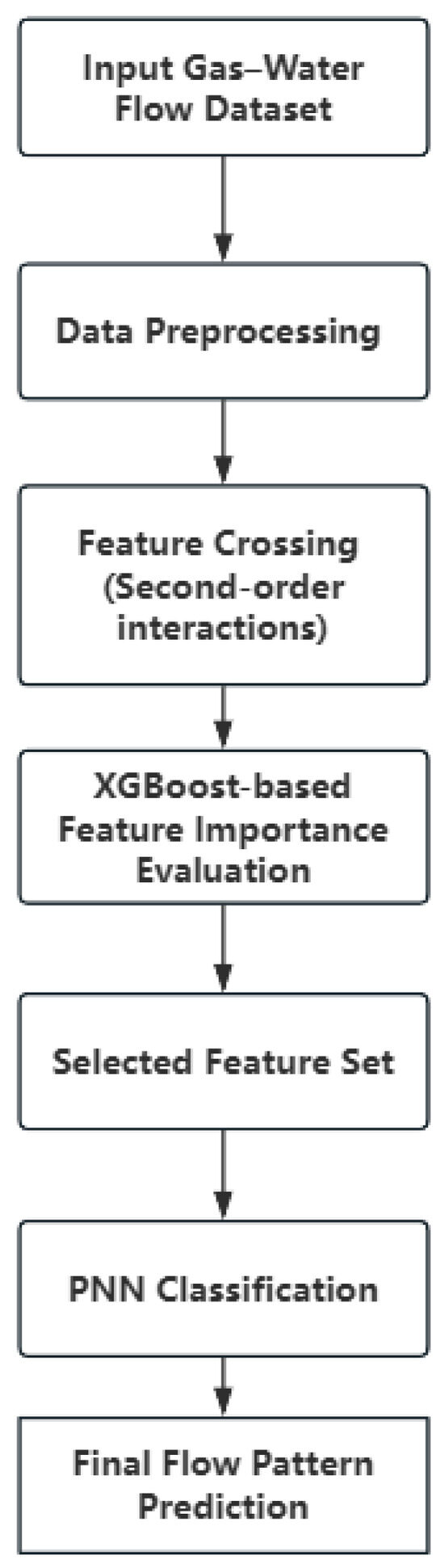
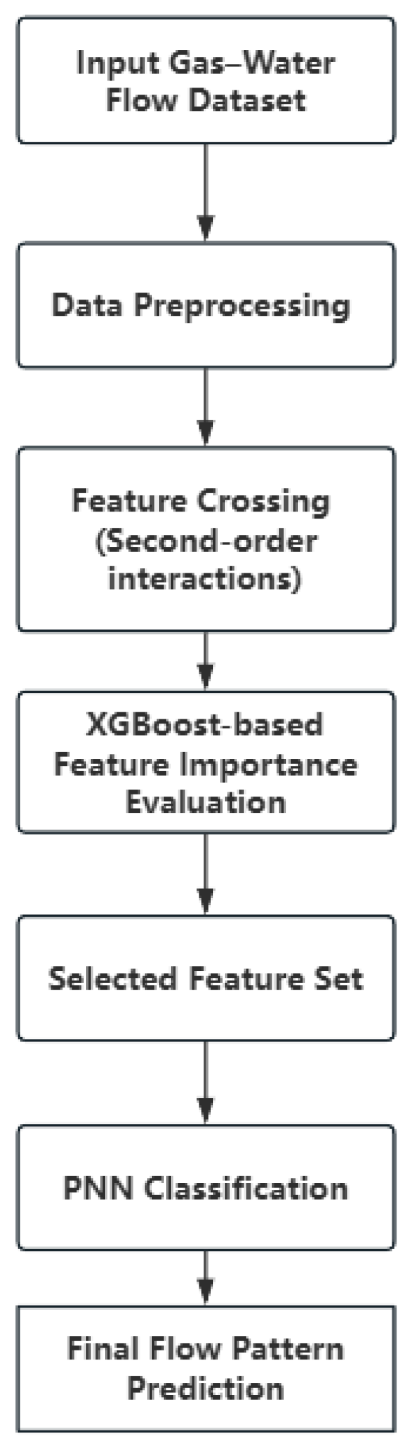
The training procedure of the hybrid model is outlined as shown in Figure 6.
Figure 6.
Two-stage feature selection and classification workflow of the proposed PNN–XGBoost framework.
Before training, we examined the raw gas–water flow dataset to check its stability and scale. The variables had different units and ranges, so we normalized all features to prevent any one variable from dominating the learning process. We started with five basic physical variables commonly used in gas–water flow studies: liquid superficial velocity, gas superficial velocity, pressure, temperature, and pipe inclination. These variables are easy to measure and have clear physical meaning. Using only them is simple but may miss interaction effects that often govern flow pattern transitions.
To capture such interactions, we used feature crossing to model combined effects, like velocity–velocity and velocity–inclination interactions. We considered using all crossed features directly but this would increase redundancy and might reduce model stability on small datasets. Therefore, we performed feature selection after crossing and kept only the most informative features.
The observed flow pattern—stratified, slug, wavy, or bubble flow—served as the output label. Labels were numerically encoded, and all selected features were normalized using min–max scaling. The dataset was first split into training and test sets with a 7:3 ratio. To check robustness, we also performed repeated random splits and 5-fold cross-validation. The model consistently showed high accuracy, with an average of 97.8% ± 0.9%, confirming its stability across different data partitions.
Next, we applied XGBoost to refine the feature set. We tried several parameter combinations and eventually chose a learning rate of 0.1, 200 estimators, and a maximum depth of 6, because this setup gave stable performance without causing overfitting. XGBoost produced feature importance scores, which we ranked from high to low. We could have kept all features, but weak ones would add noise and slow down learning. Therefore, we applied a simple threshold and removed any feature with importance below 0.05. This way, only the most informative variables and their crossed combinations were passed to the next stage, helping the PNN focus on meaningful patterns.
For the PNN, we used a Gaussian kernel to measure how similar each input was to the class prototypes. To improve performance, we set up a feedback loop: classification errors from the PNN were fed back to XGBoost, which provided heuristic, feedback-guided suggestions for adjusting the kernel smoothing parameter σ and feature weights, rather than performing explicit optimization. This adjustment process does not involve gradient-based learning or backpropagation and preserves the non-iterative nature of the PNN.
Finally, the refined features and feedback-adjusted kernel parameter were used to train the final PNN classifier. Unlike conventional ensemble methods, XGBoost does not directly participate in final prediction but functions as a feedback-driven feature and parameter guide. This cooperative yet non-ensemble design maintains structural simplicity while improving robustness.
All computations were performed on a workstation equipped with an Intel Core i7 CPU (3.6 GHz) and 32 GB RAM (Intel Corp., Santa Clara, CA, USA). No GPU acceleration was required due to the relatively small dataset size. The dataset consists of 360 samples, each characterized by five primary physical variables (liquid superficial velocity, gas superficial velocity, pressure, temperature, and pipe inclination), along with derived second-order interaction features. Model training and evaluation were implemented in Python 3.9.12 (Python Software Foundation, Wilmington, DE, USA) using standard machine learning libraries. The total training time for each model was within a few seconds. To ensure robustness, the dataset was randomly split into training and test sets with a ratio of 7:3, and 5-fold cross-validation was additionally performed. Model performance was evaluated using accuracy and Macro-F1 score.
4.5. Training Results
To enhance the representational power of the feature space, we incorporated an explicit feature crossing procedure prior to XGBoost training. Specifically, we constructed all second-order pairwise interactions among the five original input variables—liquid superficial velocity , gas superficial velocity , pressure (P), temperature (T), and pipe inclination (θ). This process yielded 10 additional interaction features, resulting in a total of 15 candidate features. The motivation stems from the physical observation that flow regime transitions in gas–liquid multiphase systems are often governed by nonlinear couplings among velocity ratios, pressure–temperature effects, and inclination-dependent gravitational forces.
The 15-dimensional feature set was then input into the XGBoost module for importance-based feature evaluation. Features with importance scores below 0.05 were removed, leading to a refined subset of 9 features (including both original and crossed terms), which were subsequently fed into the PNN classifier.
Although XGBoost can implicitly capture feature interactions through tree splits, explicit second-order construction provides several advantages under limited data conditions: (1) it reduces the required tree depth for modeling nonlinear relationships; (2) it enhances interpretability by exposing physically meaningful interaction terms; and (3) it stabilizes learning by narrowing the effective hypothesis space prior to kernel-based density estimation.
To quantitatively assess the contribution of feature crossing and XGBoost-based selection, we conducted an ablation study, as summarized in Table 2.
Table 2.
Model performance comparison.
This result also indicates that the hybrid framework does not merely increase model complexity, but effectively addresses the limitations of individual methods under small-sample conditions, thereby improving both stability and generalization. The baseline PNN trained on the original five features achieved 90.7% accuracy. Introducing explicit second-order feature crossing increased the accuracy from 90.7% to 92.3%, confirming that nonlinear couplings among flow variables carry additional discriminative information beyond individual measurements. Bayesian optimization further improved performance to 93.1%, indicating that proper kernel bandwidth selection plays a non-negligible role in density-based classification under limited data conditions.
When XGBoost-based importance selection was applied to the original five features, accuracy increased substantially to 95.4%, highlighting the critical role of boosting-based feature reweighting in suppressing weak predictors and amplifying physically dominant variables. When XGBoost was applied to the original five features, all five were retained due to their already compact structure. In contrast, when applied to the crossed feature set, nine high-importance features were preserved after removing low-importance interaction terms. Finally, combining feature crossing with XGBoost selection produced the highest performance (98.1% accuracy and 0.978 Macro-F1), indicating a clear synergistic effect.
The performance comparison in Table 2 demonstrates a clear rationale for selecting PNN-XGBoost as the final model. The standard PNN serves as a baseline, offering probabilistic outputs but suffering from sensitivity to its smoothing parameter. The PNN-BO variant addresses this by automating parameter search, yielding a more robust but computationally heavier model. The superior PNN-XGBoost model adopts a different, more effective strategy: it uses XGBoost not as a tuner, but as a powerful front-end feature selector. In our case, the XGBoost component identified and retained only the top 9 most predictive features from the original 15, effectively eliminating noise from less informative ones. This purified feature set was then classified by a standard PNN with a fixed, empirically set parameter. Thus, PNN-XGBoost’s advantage comes from its hybrid architecture—leveraging XGBoost for intelligent feature preprocessing and PNN for robust probabilistic classification—which together achieve the best generalizability on our flow pattern data.
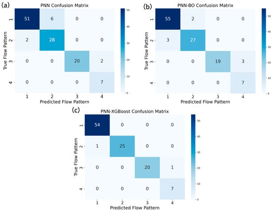
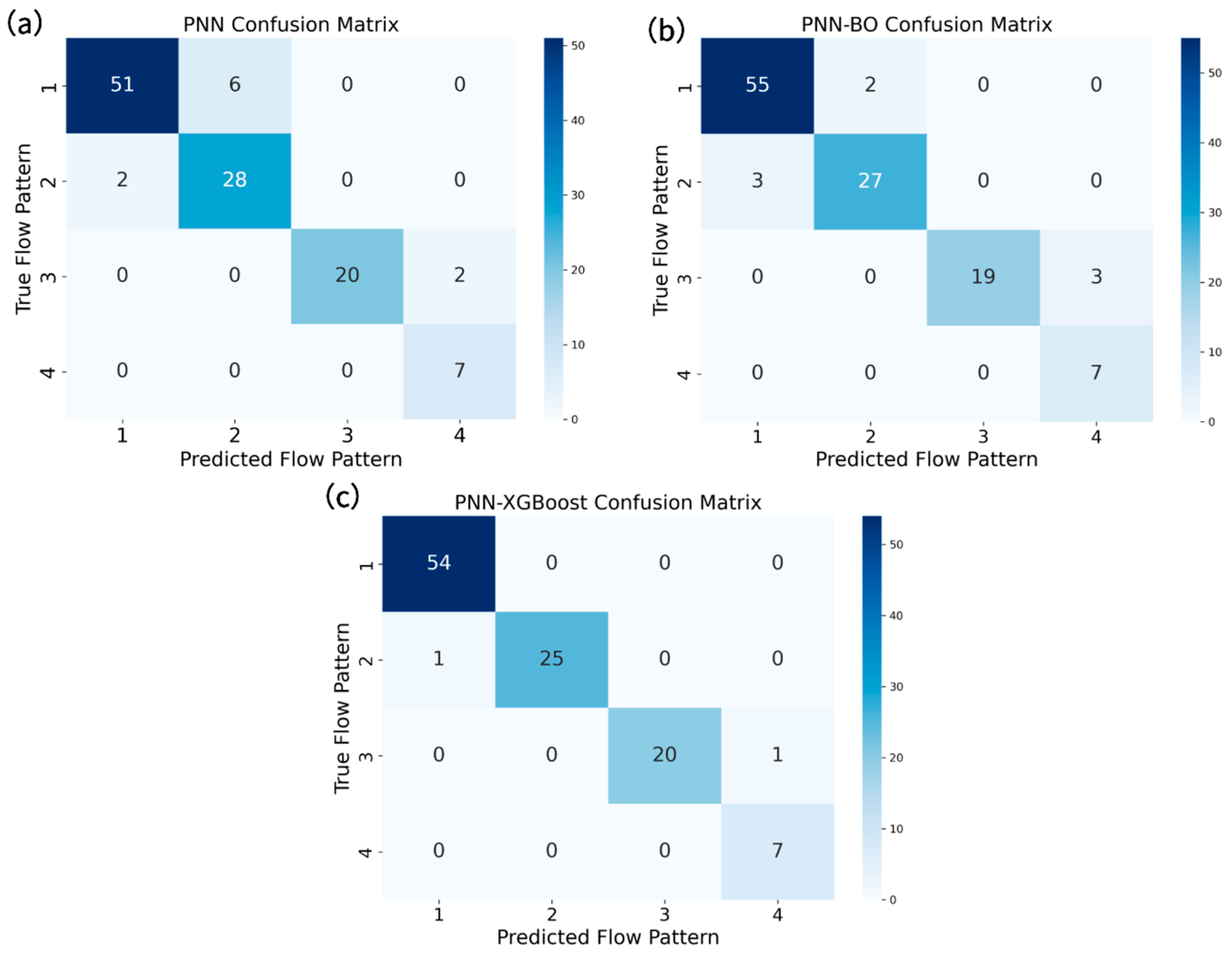
Following the workflow illustrated in Figure 6, the PNN, PNN-BO, and PNN–XGBoost models were trained and evaluated. Figure 7 presents the corresponding confusion matrices, where labels 1–4 denote bubble, slug, stratified, and wavy flows, respectively.
Figure 7.
Comparison of confusion matrices for the three classification models: (a) PNN model; (b) PNN-BO model; (c) PNN-XGBoost model.
The baseline PNN correctly identified dominant regimes but exhibited misclassification in transitional flows, particularly between slug and wavy patterns. The PNN-BO model reduced such errors through improved bandwidth tuning. The proposed PNN–XGBoost model achieved the most consistent diagonal dominance in the confusion matrix, indicating stronger discrimination of both dominant and transitional regimes.
The performance gain arises from XGBoost’s ability to highlight nonlinear relationships among key physical features—such as phase velocity ratios and inclination-modulated holdup variations—combined with PNN’s smooth probabilistic classification. This integration enhances sensitivity, reduces false negatives, and significantly strengthens flow pattern recognition in near-horizontal wells.
4.6. Model Validation
To accurately identify the actual gas–water flow patterns within the wellbore and gain deeper insights into the downhole fluid dynamics, this study employs array logging tools for data acquisition and analysis in a field case. The fiber-optic probes installed on the array tool exhibit low responses in water and high responses in gas, and can detect the number of gas bubbles passing through, thereby providing high-resolution spatial information for flow pattern recognition [31].
Based on the measured responses at four points on the wellbore cross-section, inverse distance interpolation is applied to generate 24 approximate circumferential points. These are visualized through color mapping to construct a cross-sectional fluid distribution image, enabling intuitive spatial validation of the model prediction results.
However, conventional 2D plots are limited in capturing the spatial structure of flow patterns within the wellbore. To address this, a 3D visualization system is further developed using fiber-optic probe data. Well depth is mapped to the Z-axis, while X/Y spatial coordinates are constructed based on the well trajectory. The predicted flow patterns are then superimposed on the 3D wellbore model using color encodings (e.g., yellow for gas, blue for liquid) and volume indicators, thereby providing a comprehensive and intuitive representation of the gas–water flow status within the wellbore.
Through this 3D visualization system, the evolution of predicted flow patterns along different well depths is further analyzed. The visualized results clearly reveal the non-uniformity of flow regimes along the vertical axis, with certain depth intervals exhibiting abrupt transitions, such as from bubbly flow to slug flow. These transition zones are difficult to identify in conventional 2D formats but are prominently highlighted in the 3D model through color discontinuities and structural boundaries, offering valuable support for locating flow regime transition bands or potential production zones.
To validate the practical applicability of the proposed flow pattern prediction model in real wells and to enhance the interpretability and intuitiveness of the prediction results, this study selects a gas–water two-phase horizontal well (Well A) as the research subject to conduct an application analysis using field measurement data, further demonstrating the model and visualization system’s value in engineering practice. Well A is a gas–water two-phase horizontal well with an internal diameter of 99.56 mm, a maximum inclination of 91.3°, downhole fluid temperatures of 102.5–105 °C, and downhole pressures of 29.4–30.4 MPa. Field measurements indicated that the flow pressure was below the bubble-point pressure, implying that the gas phase existed as free gas. Logging data from the production interval at depths of 3579–4887 m (total length 1308 m) were selected. Under a production rate of 80,000 m3/d, two logging runs were carried out at cable speeds of 20 m/min and 15 m/min. Recorded parameters included deviation (DEV), temperature (TEMP), pressure (PRESS), and fiber-optic signal (FGS); and from these, true vertical depth (TVD) and water holdup (HoldUpWater) curves were derived.
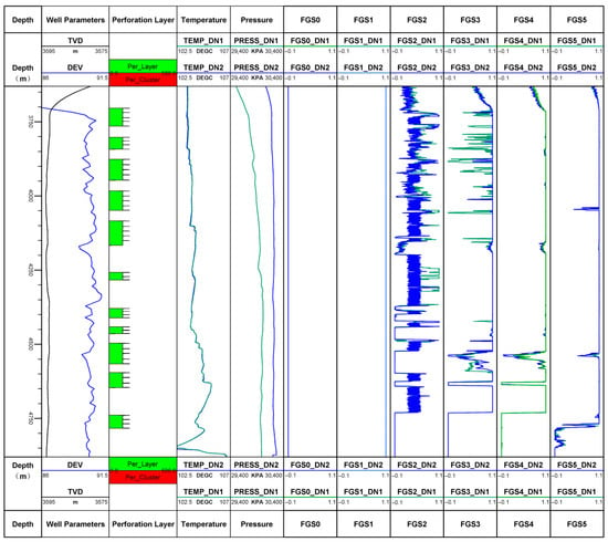
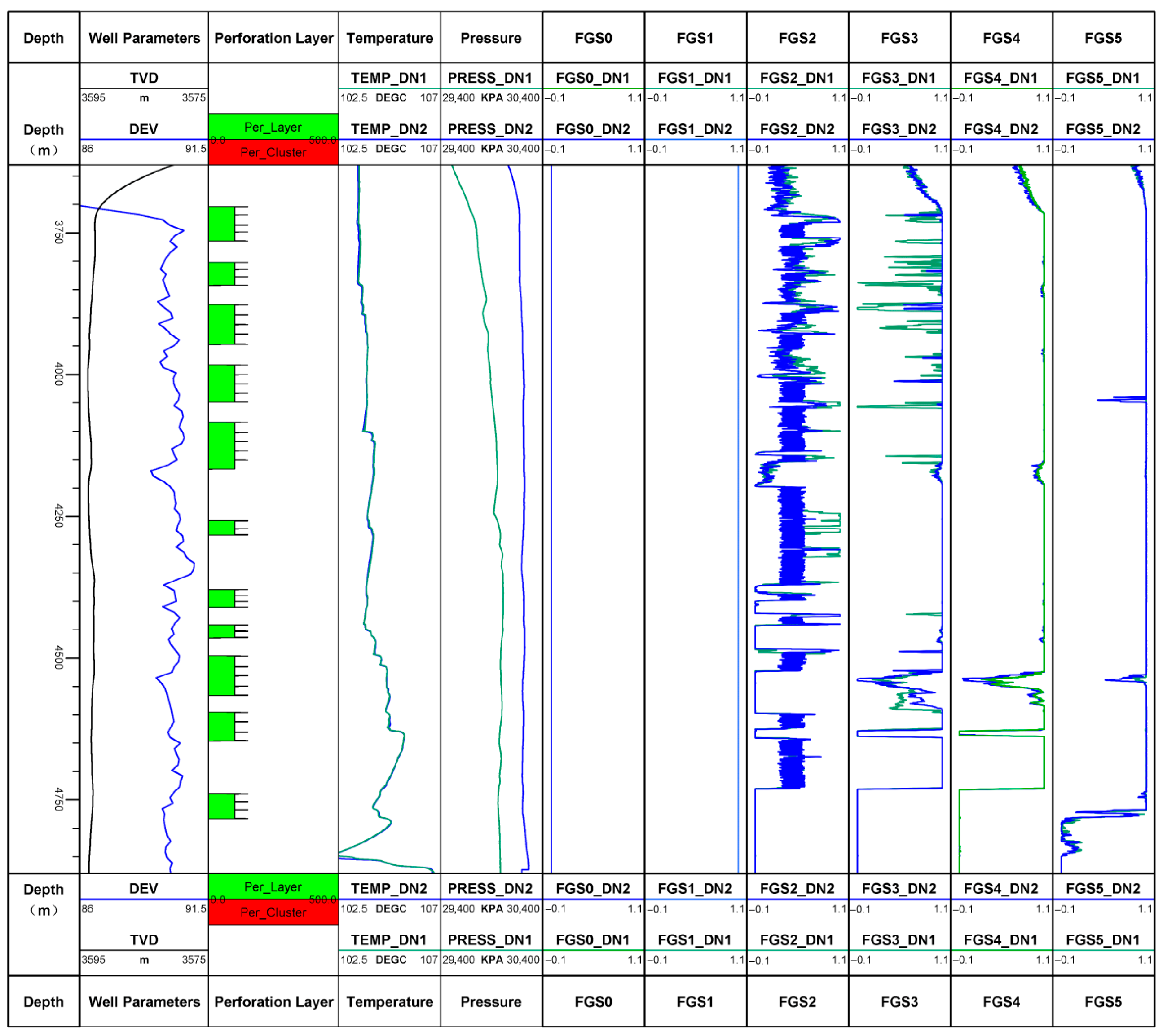
Local flow velocities were first computed by using the turbine-intersection method, and average velocities were then obtained via the integral method, as previously described in. Average gas holdup was calculated from the fiber-optic probe responses, and interpolation was applied to generate holdup images (gas in yellow, water in blue), following the methods in [32]. A stratified-flow model was subsequently used to determine a downhole gas flow rate of 431.83 m3/d for the entire flow zone. After PVT correction, the corresponding surface production rates were 81,408.21 m3/d for gas and 84.13 m3/d for water. The logging-curve playback is shown in Figure 8.
Figure 8.
Playback of logging-tool measurement curves for Well A.
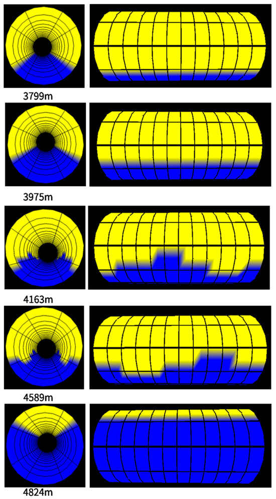
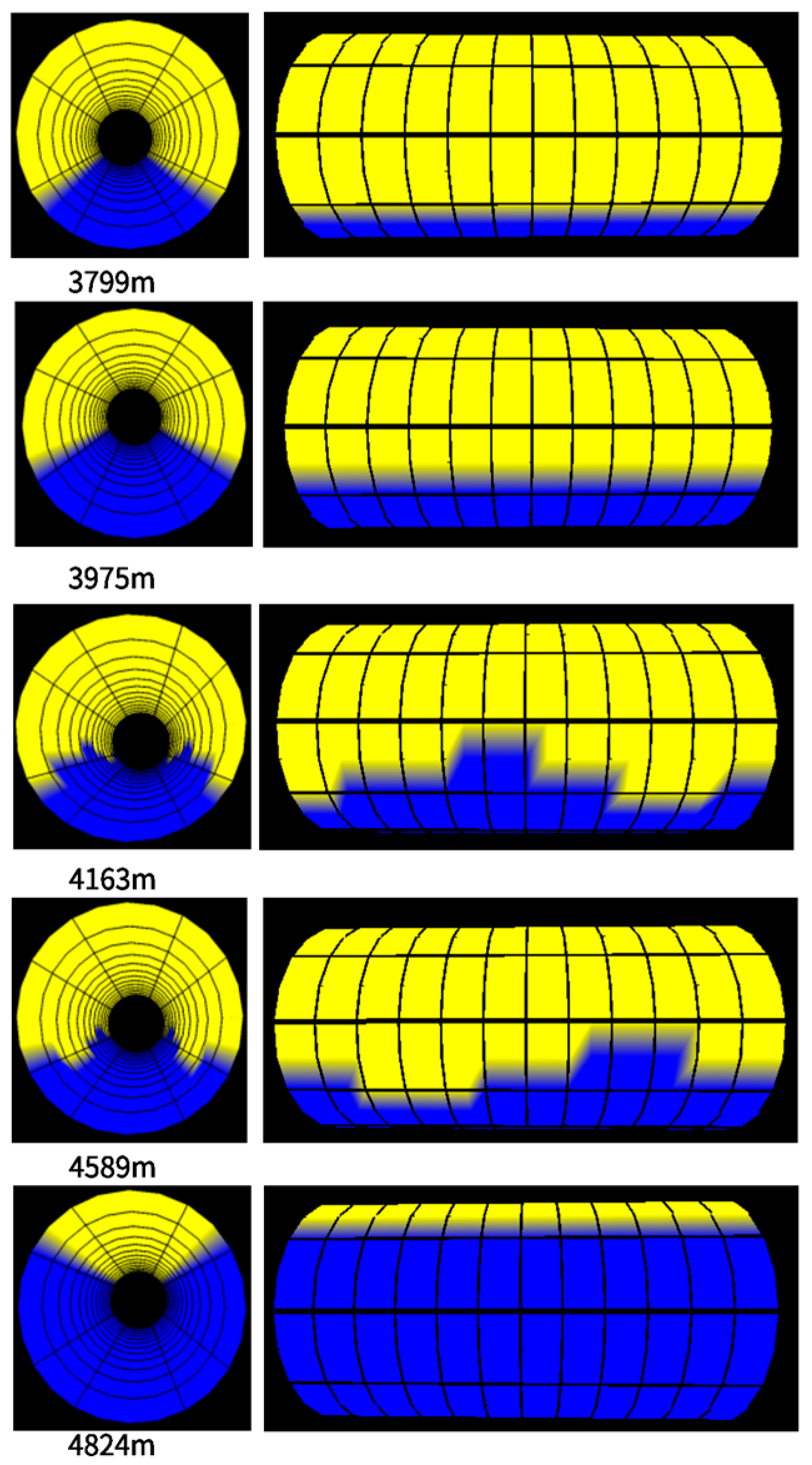
Based on an interpretation of actual wellhead production and production-profile logs, five representative production intervals, each characterized by distinct inclination angles and flow rates, were selected for further analysis. Three-dimensional holdup images, inverted from fiber-optic probe measurements, were visualized from multiple perspectives to intuitively depict fluid migration patterns within each interval (Figure 9).
Figure 9.
Three-dimensional holdup images of flow patterns in Well. The image volume is color-coded to represent the phase holdup distribution: blue indicates water, and yellow indicates gas.
To verify the effectiveness of the proposed methodology, flow-pattern distribution patterns were preliminarily classified by using a scatter-matrix plot; and subsequently, the PNN-XGBoost prediction model introduced herein was applied to the sample data for flow-pattern identification. The results are presented in Table 3.
Table 3.
Comparison of actual and predicted flow patterns in Well A.
First, by referring to the flow-pattern scatter plot in Figure 3 and considering the inclination angles and phase flow rates of the five intervals listed in Table 3, the patterns were identified as stratified, stratified, wavy, wavy, and stratified flow, respectively. Next, comparison with the water-holdup images inverted from fiber-optic probe data confirmed that these patterns matched the scatter-diagram predictions. Finally, inclination angle, phase flow rates, superficial velocities, fluid densities, temperature, and pressure were input into the prediction models. The results show that the PNN-BO model still exhibited deviations when predicting stratified flow, whereas the PNN-XGBoost model’s outputs were fully consistent with the actual flow patterns. This demonstrates that the PNN-XGBoost model achieves satisfactory predictive accuracy in Well A, meeting the precision requirements for practical production applications.
From an operational perspective, the model can be integrated into production logging workflows as a preprocessing or auxiliary module. Specifically, real-time or post-processed measurement data can be input into the trained model to obtain continuous flow pattern predictions along the wellbore. These predicted flow regimes can then serve as physically meaningful constraints or prior information for subsequent interpretation tasks, such as phase holdup estimation, flow profile reconstruction, and PVT property inversion. In this way, the model does not replace traditional interpretation methods, but rather complements them by improving the stability and reliability of inverse analysis, particularly in scenarios where direct flow visualization is not available. This integration highlights the practical applicability of the proposed approach in real oilfield scenarios, especially for fiber-optic monitoring and array-based logging systems.
5. Conclusions
In the gas–water two-phase simulation experiments in horizontal wellbores, which were carried out at inclination angles of 90°, 88°, 85°, and 83°, four flow patterns, namely, stratified, wavy, slug, and bubble flows, were identified. Scatter-matrix analysis revealed distinct boundaries among these patterns, although their spatial distributions varied under different conditions.
Based on the experimental flow pattern data, a PNN–XGBoost model incorporating explicit second-order feature crossing and XGBoost-based feature selection was trained to learn the nonlinear relationships between flow patterns, well deviation angles, and phase flow rates of gas and water. The model successfully achieved accurate flow pattern prediction under various experimental conditions. Furthermore, the model was applied to flow pattern prediction using field data from a case well, demonstrating favorable predictive performance. These results indicate that the proposed model has strong potential for practical application in production operations and can provide valuable support for well logging interpretation.
In addition, a three-dimensional visualization system was developed in this study to overcome the limitations of traditional two-dimensional plots. This system intuitively displays the spatial distribution of flow patterns within the wellbore, significantly enhancing the credibility of the model predictions and improving the interpretability and operational usability of the results.
Since only four patterns were observed under the current experimental conditions, future work should include additional two-phase flow simulation experiments at a broader set of inclination angles. This expansion will enable the comprehensive prediction of gas–water flow patterns for arbitrary combinations of inclination angle and flow rate.
Author Contributions
Conceptualization, T.L. and J.L.; methodology, T.L.; software, T.L.; validation, T.L., J.L., Y.C. and R.Y.; formal analysis, T.L.; investigation, T.L.; resources, J.L. and T.Z.; data curation, T.L., T.Z. and Z.Z.; writing—original draft preparation, T.L.; writing—review and editing, T.L. and J.L.; visualization, T.L.; supervision, J.L.; project administration, J.L.; funding acquisition, J.L. All authors have read and agreed to the published version of the manuscript.
Funding
This research was funded by the Open Fund of Key Laboratory of Exploration Technologies for Oil and Gas Resources (Yangtze University), Ministry of Education, grant number K2018-10.
Data Availability Statement
The original contributions presented in the study are included in the article. Further inquiries can be directed to the corresponding author.
Acknowledgments
The authors would like to thank the editors and the anonymous reviewers for their insightful and constructive comments.
Conflicts of Interest
The authors declare that they have no known competing financial interests or personal relationships that could have appeared to influence the work reported in this paper. Author Tianjun Zhang and Author Zhongliang Zhao are employees of Qinghai Oilfield Testing Company of Petro China. The remaining authors declare no conflicts of interest.
Abbreviations
The following abbreviations are used in this manuscript:
| CFD | Computational Fluid Dynamics |
| AI | artificial intelligence |
| BP | backpropagation |
| SSA-BP | sparrow-search-algorithm-optimized BP |
| PNNs/PNN | probabilistic neural networks |
| CNNs | convolutional neural networks |
| LSTMs | long short-term memory networks |
| XGBoost | eXtreme Gradient Boosting |
| BO | Bayesian Optimization |
| Vsw | superficial water velocity |
| Vsg | superficial gas velocity |
| BF | bubble flow |
| SL | slug flow |
| SS | stratified flow |
| SW | wavy flow |
| θ | pipe inclination |
| DEV | deviation |
| TEMP/T | temperature |
| PRESS/P | pressure |
| FGS | fiber-optic signal |
| TVD | true vertical depth |
| HoldUpWater | water holdup |
| PVT | Pressure-Volume-Temperature |
References
- Bao, M.; Wang, M.; Li, K.; Jia, X. Integrating machine learning with sensor technology for multiphase flow measurement: A review. IEEE Sens. J. 2024, 24, 29603–29618. [Google Scholar] [CrossRef] [Scilit]
- Li, M.; Liu, J.; Xia, Y. Risk prediction of gas hydrate formation in the wellbore and subsea gathering system of deep-water turbidite reservoirs: Case analysis from the South China Sea. Reserv. Sci. 2025, 1, 52–72. [Google Scholar] [CrossRef] [Scilit]
- Ali, J.; Ansari, U.; Ali, F.; Javed, T.; Hullio, I.A. Application of machine learning for effective screening of enhanced oil recovery methods. Reserv. Sci. 2026, 2, 65–80. [Google Scholar] [CrossRef] [Scilit]
- Tian, L.; Zhang, Q.; Li, X.; Li, C. Fracturing effectiveness evaluation based on flowback data using pressure transient testing. Reserv. Sci. 2026, 2, 97–110. [Google Scholar] [CrossRef] [Scilit]
- Hu, H.; Liu, J.; Fu, R.; Luan, X.; Zhou, S. Data analysis and model establishment of oil–water two-phase in vertical well based on array probe combination instrument. Prog. Geophys. 2022, 37, 1732–1741. [Google Scholar]
- Shi, S.; Liu, J.; Hu, H.; Zhou, H. A research on a GA-BP neural network based model for predicting patterns of oil–water two-phase flow in horizontal wells. Geoenergy Sci. Eng. 2023, 230, 212151. [Google Scholar] [CrossRef] [Scilit]
- Liu, J.; Xu, Y.; Wu, Q. Holdup flow imaging analysis for capacitance and resistance ring array probes. Prog. Geophys. 2018, 33, 2141–2147. [Google Scholar]
- Zhang, Z.; Jin, N.; Bai, L.; Dai, L.; Ren, W.; Wei, J. Nonlinear analysis for identification of vertical upward oil–water two-phase flow patterns. IEEE Sens. J. 2023, 24, 3259–3265. [Google Scholar] [CrossRef] [Scilit]
- Mandhane, J.M.; Gregory, G.A.; Aziz, K. A flow pattern map for gas–liquid flow in horizontal pipes. Int. J. Multiph. Flow 1974, 1, 537–553. [Google Scholar] [CrossRef] [Scilit]
- Liu, J.; Guo, H.; Wang, J.; Du, W.; Xue, W. Experimental study of flow patterns of oil–gas–water three-phase flow in large-diameter horizontal tubing. J. Pet. Technol. 2010, 32, 87–91. [Google Scholar]
- Cui, S.; Liu, J.; Chen, X.; Li, Q. Experimental analysis of gas holdup measured by gas array tool in gas–water two phase of horizontal well. Coatings 2021, 11, 343. [Google Scholar] [CrossRef] [Scilit]
- Niu, Y. Numerical Simulation and Experimental Study of Gas–Water Two-Phase Flow Pattern in Horizontal Wells. Master’s Thesis, Changjiang University, Jingzhou, China, 2022. [Google Scholar]
- Liu, Y.; Luo, C.; Liu, T.; Ren, G.; Wang, Z. Prediction of gas–liquid two-phase flow patterns in horizontal gas wells. J. Southwest Pet. Univ. (Sci. Technol. Ed.) 2019, 41, 107–112. [Google Scholar]
- Zhao, X.; Song, H.; Wang, M.; Zhang, X.; Li, Y.; Wang, X. Research on flow pattern identification method of logging in horizontal well gas–water two-phase production based on artificial intelligence algorithm. Mod. Chem. Res. 2023, 43, 173–175. [Google Scholar]
- Wu, X. Progress of flow image logging research. Prog. Geophys. 2002, 18, 272–276. [Google Scholar]
- Akhnoukh, R.; Leighton, J.; Bigno, Y.; Bouroumeau-Fuseau, P.; Quin, E.; Catala, G.; Silipigno, L.; Hemingway, J.; Horkowitz, J.; Hervé, X.; et al. Keeping producing wells healthy. Oilfield Rev. 1999, 11, 30–47. [Google Scholar]
- Syikilili, A.M.; Nydal, O.J.; Kimambo, C.Z.; Kihedu, J.H. Effect of pipeline inclination on multiphase flow. Exp. Comput. Multiph. Flow 2021, 4, 377–388. [Google Scholar] [CrossRef] [Scilit]
- Li, L.; Wang, X.; Liu, S.; Liu, J.; Gao, Y.; Li, C. Gas–water flow law in horizontal wellbore and its influencing factors. Acta Pet. Sin. 2019, 40, 1244–1254. [Google Scholar] [CrossRef]
- Song, H.; Guo, H.; Dai, J. Experimental analysis of gas–water flow pattern during production well logging in horizontal wells. J. Pet. Technol. 2011, 33, 96–101. [Google Scholar]
- Srivastava, N.; Hinton, G.; Krizhevsky, A.; Sutskever, I.; Salakhutdinov, R. Dropout: A simple way to prevent neural networks from overfitting. J. Mach. Learn. Res. 2014, 15, 1929–1958. [Google Scholar]
- Andayani, U.; Sumantri, I.B.; Arisandy, B. Classification of zingiber plants based on stomate microscopic images using probabilistic neural network (PNN) algorithm. J. Phys. Conf. Ser. 2020, 1566, 012122. [Google Scholar] [CrossRef] [Scilit]
- Porwik, P.; Doroz, R.; Orczyk, T. Signatures verification based on PNN classifier optimised by PSO algorithm. Pattern Recognit. 2016, 60, 998–1014. [Google Scholar] [CrossRef] [Scilit]
- Wang, R.; Zhao, H.; Hua, D.; Li, J.; Wang, X.; Ji, F. A virtual impactor-based portable optical sensor with probabilistic neural network: For particle property identification. IEEE Sens. J. 2023, 23, 14512–14521. [Google Scholar] [CrossRef] [Scilit]
- Zhang, R.; He, Z.; Chen, W.; Li, Z.; Hao, J. Classification and recognition of fresh Lentinus edodes with machine vision image processed by Bayesian hyperparametric optimization technology. J. Hebei Agric. Univ. (Nat. Sci. Ed.) 2024, 47, 116–123. [Google Scholar]
- Gupta, V.K.; Lalwani, S.K.; Bhati, G.S.; Prakash, S.; Sunny. Bayesian optimization based neural architecture search for classification of gases/odors mixtures. IEEE Sens. J. 2024, 24, 7119–7125. [Google Scholar] [CrossRef] [Scilit]
- Yuan, H.; Ji, S.; Li, H.; Zhu, C.; Zou, Y.; Ni, B.; Gu, Z. Classification forecasting research of rock burst intensity based on the BO-XGBoost-Cloud model. Earth Sci. Inform. 2025, 18, 95. [Google Scholar] [CrossRef] [Scilit]
- Fan, Z.; Song, W.; Ke, Y.; Jia, L.; Li, S.; Li, J.J.; Zhang, Y.; Lin, J.; Wang, B. XGBoost-SHAP-based interpretable diagnostic framework for knee osteoarthritis: A population-based retrospective cohort study. Arthritis Res. Ther. 2024, 26, 213. [Google Scholar] [CrossRef] [Scilit]
- Kumar, A.; Barath, J.K.; Shanmukh, P.; Joshi, D. StreXNet: A novel end-to-end deep learning based improved multi-level mental stress classification from EEG sensors. IEEE Sens. J. 2024, 25, 3538–3551. [Google Scholar] [CrossRef] [Scilit]
- Zhou, H.; Liu, J.; Guo, H.; Cui, S.; Hu, H.; Luo, W.; Li, Y.; Shi, S. Research on the imaging algorithm of oil–water two-phase interface in horizontal wells based on arrayed electrical resistance probes. IEEE Sens. J. 2023, 24, 3693–3702. [Google Scholar] [CrossRef] [Scilit]
- Zhuang, X.; Zhou, D.; Jia, Y.; Liu, S.; Liang, J.; Lin, Y.; Hou, H.; Qian, D.; Zhou, T.; Bai, X.; et al. Bottom-up defect modification through oily-allicin modified buried interface achieving highly efficient and stable perovskite solar cells. Adv. Mater. 2024, 36, 2403257. [Google Scholar] [CrossRef] [Scilit]
- Zhou, H.; Liu, J.; Fei, J.; Shi, S. A model based on the random forest algorithm that predicts the total oil–water two-phase flow rate in horizontal shale oil wells. Processes 2023, 11, 2346. [Google Scholar] [CrossRef] [Scilit]
- Li, J.; Ma, H.; Hou, Z.; Wu, X.; Song, W.; Guo, H. Development and application of MAPS 3D borehole imaging software based on C#+OpenGL. J. Yangtze Univ. (Nat. Sci. Ed.) 2024, 21, 101–109. [Google Scholar]

Disclaimer/Publisher’s Note: The statements, opinions and data contained in all publications are solely those of the individual author(s) and contributor(s) and not of MDPI and/or the editor(s). MDPI and/or the editor(s) disclaim responsibility for any injury to people or property resulting from any ideas, methods, instructions or products referred to in the content. |
© 2026 by the authors. Licensee MDPI, Basel, Switzerland. This article is an open access article distributed under the terms and conditions of the Creative Commons Attribution (CC BY) license.