AI-Based Wind Tracking and Yaw Control System for Optimizing Wind Turbine Efficiency

Abstract

Accurate yaw alignment is critical for maximizing power capture in horizontal-axis wind turbines, as even moderate yaw misalignment leads to significant aerodynamic losses, increased actuator usage, and accelerated mechanical wear. This research paper proposes a hybrid smart yaw control system for small-scale wind turbines that combines real-time measurements with short-term wind direction prediction to improve alignment accuracy, operational reliability, and energy efficiency under realistic operating conditions. The system integrates four wind direction information sources, such as physical wind vane sensing, live online weather data, forecast data, and a data-driven prediction module within a structured priority framework (VANE → LIVE → FORECAST → AI), to ensure continuous yaw control during sensor or communication unavailability. The prediction module is based on a long short-term memory (LSTM) neural network trained in MATLAB using live data from an online platform, with sine–cosine encoding employed to address the circular nature of directional data. The yaw controller incorporates a ±15° deadband, dwell-time logic, shortest-path rotation, and cable-safe constraints to reduce unnecessary actuation while maintaining effective alignment. The proposed system is validated through MATLAB/Simulink simulations and real-time microcontroller-based experiments using a stepper motor-driven nacelle. Compared with conventional vane-based yaw control, the hybrid AI-assisted approach reduces the average yaw error by approximately 35–45%, maintains a yaw error within ±15° for more than 90% of the operating time, increases average electrical power output by 3–5%, and reduces yaw motor energy consumption by 10–15%, while decreasing corrective yaw actuation events by 30–40%. These results demonstrate that integrating an LSTM-based wind direction predictor with multi-source wind data provides a robust, low-cost, and practically deployable yaw control solution that enhances energy capture and mechanical durability in small-scale wind turbines.

1. Introduction

Wind energy use has been increasing rapidly and steadily across the world. The Global Wind Energy Council says that this increase is due to supporting policies, less barriers to entry into the market, and wind power’s rising role in global efforts to reduce carbon emissions [1]. Horizontal-axis wind turbines (HAWTs) are the most common type of wind turbine used today. These turbines have an upwind rotor design and strong structural framework, which make them highly reliable for wind energy applications. Also, these turbines can be easily scaled for use in both large utility-scale wind farms and smaller community-based systems [2]. To get maximum output from a HAWT, one of the most important things to do is to get the yaw alignment right so that the rotor faces the wind as directly as possible. Even small yaw offsets make the effective velocity component normal to the rotor plane weaker. This causes power to drop in a way that follows the well-known cosine-cubed relationship $P\propto {cos}^3\theta$ [3].

Yaw misalignment has been extensively researched because of its significant impact on turbine efficiency and structural loads. Liew et al. showed that a rotor’s cosine cubed sensitivity to yaw angle causes major power losses even when the rotor is only slightly out of line [4]. Wang and Liu’s [5] recent study showed that uncorrected yaw errors can also cause higher fatigue loads, in addition to static aerodynamic effects. This shows how important it is to keep alignment within a controlled tolerance range. Gao et al. [6] introduced a data-driven methodology for rectifying yaw misalignment, using operational turbine data to find and correct yaw biases, therefore improving performance and reducing mechanical stress. Astolfi et al. [7] developed an advanced diagnostic approach for detecting systematic yaw errors from nacelle-anemometer data, allowing a more reliable diagnosis of long-term misalignment.

A secondary principal area in yaw control research relates to sensor reliability and the accuracy of directional measurement. Small errors in yaw angle sensors can introduce a persistent measurement bias, leading the controller to detect a false misalignment and trigger unnecessary yaw rotations. Pei et al. [8] addressed this issue by applying a data-driven method to detect yaw sensor zero-point drift, and the results highlight the need for reliable directional sensing. Mittelmeier and Kuhn [9] developed an SCADA-based method that improves yaw alignment by using filtered nacelle measurements and averaging logic, and their work shows that careful processing of standard sensor data can greatly reduce unnecessary or incorrect yaw movements Later, Liu et al. [10] made yaw error correction better by utilizing combined adaptive estimates and control logic. The result made it so that the misalignment remains the same even when the wind changed.

Adaptive and self-tuning yaw strategies have become increasingly common alongside traditional sensing methods. Saenz-Aguirre et al. [11] introduced a self-tuning yaw control technique that adjusts its parameters as wind conditions change which improves alignment stability compared with fixed-parameter approaches. Bu et al. [12] highlighted the importance of structured yaw algorithms and showed that micro-stepping motor control and clearly defined yaw error thresholds can improve tracking accuracy and reduce overshoot when implemented using DSP-based control. Reinforcement learning methods have also been explored. Kadoche et al. [13] applied multi-agent reinforcement learning to improve yaw control across a wind farm. Puech and Read [14] used RL-based optimization on a single turbine. After that, Al-Rubaye and Gil-Pita [15] proposed an optimization method that considers both turbine placement and yaw angle estimation at the farm level, demonstrating that coordinated decisions can significantly increase power capture. Anagnostopoulos et al. [16] developed machine learning models with several accuracy levels for real-time yaw control on multiple turbines. Yang et al. [17] showed how yaw systems have gradually developed over time, moving from simple passive tailvane mechanisms to more advanced electromechanical designs that rely on modern sensors and improved control methods. Early experimental work by Wu and Wang [18] also supported this shift. Their tests on small horizontal-axis wind turbines (HAWTs) found that active electromechanical yaw systems provide much better stability than traditional passive setups. Recently, Islam et al. [19] proposed an intelligent yaw mechanism that use machine learning to minimize reliance on costly directional sensors by statistically calculating wind direction.

For small turbines, commercial yaw systems are often too large or costly to be practical. As a result, researchers have explored low-cost, microcontroller-based yaw solutions instead. Joshi and Soni [20] confirmed an economical active yaw mechanism employing stepper motor actuation and deadband logic. Kerling and Zimmer [21] proposed a cost-sensitive yaw control technique that initiates modifications just when anticipated energy benefits surpass actuation expenses. There have also been reports of designs that emphasize robustness. Bu et al. [12] improved previous yaw algorithms to reduce oscillatory behavior. Tsioumas et al. [22] created an indirect estimation method for yaw misalignment using operational data. Shahadat et al. [23] indicated that active yaw tracking can greatly improve small turbines, and Abhi et al. [24] showed that microcontroller-based yaw control that is in sync with real-time wind inputs can significantly improve responsiveness and reliability.

Following this development, predictive and data-driven methods have improved yaw control even further. Yin and Zhao [25] created a prediction model for offshore turbines based on LSTM, which improved alignment when the wind changed quickly. This approach complements the multi-source smart yaw control system introduced, where predictions from an AI model are integrated with live measurements and forecast data to improve performance. Also, Ang et al. [26] proposed a wind direction prediction approach for yaw systems for short-term prediction models that can improve alignment decisions during rapidly changing wind conditions.

Rott et al. [27] introduced a wind vane correction method designed to reduce misalignment and improve the accuracy of yaw decisions in horizontal-axis wind turbines. Santoni et al. [28] applied a data-driven machine learning approach to support yaw control at the wind farm level that shows that predictive coordination can improve overall performance. Elkodama et al. [29] studied yaw strategies for a twin-rotor 10 MW turbine and found both challenges and the potential of achieving precise control in large-scale systems. Liu et al. [6] focused on minimizing remaining yaw error values by combining adaptive estimation with control logic under changing wind conditions.

Although there is significant advancement in yaw control strategies, there are still a number of issues that are yet to be solved, especially in the case of small-scale horizontal-axis wind turbines. Traditional, yaw control systems continue to heavily depend on single-source directional measurements, e.g., wind vanes or sensors mounted on the nacelle, which are prone to noise, mechanical degradation, calibration drift and low response at low wind speeds. Even though the recent data-driven and machine learning-based approaches have enhanced yaw error estimation and fault detection methods, many existing approaches are founded on the assumption of a static regression model or rule-based reasoning that does not explicitly consider the temporal dynamics of wind behavior. Consequently, such approaches tend to be slow to respond to sudden changes in wind direction and temporary changes, and therefore propagate late reactions or less than optimal yaw reactions. Yaw control strategies using reinforcement learning (RL) have also been studied, mostly at the wind farm scale, but generally need a large training set, long exploration times and highly scaled computations. The practicality of RL-based approaches to low-cost microcontroller environments and to single small-scale turbines is not feasible, since these requirements are not met.

Compared to this, the majority of established LSTM-based yaw control studies assume large-scale or offshore turbines and do not often consider realistic problems such as the reliability of multi-source data and fallback operation when one or more of the sensors or communicators fail and the actuator-level limitations in small-scale systems. To address these gaps, this paper will suggest a hybrid smart yaw control system of small horizontal-axis wind turbines that uses physical wind vane measurements, real-time online weather data, forecast data, a short-term LSTM-based wind direction prediction model, and a prioritized hierarchy (VANE > LIVE > AI > FORECAST). In contrast to the traditional yaw control methods or the fully AI-based solutions, the introduced framework guarantees permanent yaw action in the event of data source failures, as well as the explicit adoption of yaw deadband logic, dwell-time conditions, cable-safe limits and yaw-contingent power estimation. The paper has introduced methodological novelty, as well as quantified performance benefits, through a realistic power curve founded on a manufacturer-, yaw- and wind speed-dependent dynamic power coefficient, which yields a robust, practical and deployable yaw control solution to small-scale wind turbines that operate in varying wind conditions.

2. Methodology

The suggested AI-driven smart yaw control system is executed in accordance with the organized workflow scheme shown in Figure 1, which illustrates the entire cycle of wind data reception to closed-loop feedback. The design of the methodology will ensure the effective nacelle alignment to the different wind conditions and reduce unnecessary yaw actuation and mechanical wear.

This workflow starts with the wind data input, in which the wind direction and wind speed are obtained form in four sources, for example, a physical wind vane attached to the turbine, live online weather data through an application programming interface (API), forecast wind data, and a short-term prediction model based on AI. Multiple sources make it more robust and permit the system to continue functioning even in the presence of sensor failures or communication failures. Any signal of wind direction is standardized between the range of 0 and 360.

Next, source selection is performed using a priority-based logic defined as VANE > LIVE > FORECAST > AI. The wind vane is preferred because it provides direct on-site measurements with minimal latency. If the vane becomes unavailable or unreliable, the controller switches to live online data. Forecast data is used when both vane and live inputs are unavailable, while the AI-predicted wind direction serves strictly as a fallback when no physical or online measurements exist. This hierarchy ensures reliable control while limiting unnecessary reliance on prediction.

Once a valid wind reference is selected, the controller computes the yaw error, defined as the angular difference between the selected wind direction and the current nacelle heading measured by a magnetic encoder. The yaw error is wrapped within ±180° to avoid discontinuities at angular boundaries and to ensure that the shortest rotational path is always selected.

The yaw error is then evaluated under control conditions. Yaw actuation is enabled only when the wind speed exceeds 3.5 m/s, the absolute yaw error is greater than or equal to ±15°, and the error persists for at least 180 s. These conditions prevent unnecessary yaw motion during low-wind operation, filter out short-term fluctuations, and balance aerodynamic efficiency against mechanical wear.

When the conditions are satisfied, yaw actuation is initiated. The nacelle is rotated using a stepper motor along the shortest path either clockwise or counterclockwise, while enforcing a cable-safe constraint to prevent excessive twisting beyond ±180°. Following alignment, power estimation is performed using a yaw- and wind speed-dependent power coefficient combined with the manufacturer’s power curve. Finally, a feedback and loop update stage continuously updates the yaw position, power output, and source status, forming a closed-loop control system that adapts dynamically to changing wind conditions.

2.1. Energy Available in the Wind

Wind energy is a natural and renewable source that can be used to create power. A wind turbine does this by transferring the kinetic energy of moving air into electricity. Figure 2 illustrates the swept area of the wind turbine, which plays an important role in determining how much wind energy the turbine can capture. The amount of power a turbine makes depends on a few important things, such as the density of the air, the speed of the wind, and the size of the area that the blades sweep.

The kinetic energy of a unit mass of moving air is given by the following formula:

$$E_k={\displaystyle \frac{1}{2}}m{v}^2$$

(1)

where $m$ is the mass of the air and $v$ is its velocity.

Considering the air density $\mathsf{\rho }$, and the cross-sectional area A swept by the turbine blades, the total available power in the wind flowing through that area becomes

$$P={\displaystyle \frac{1}{2}}\mathsf{\rho }A{v}^3.$$

(2)

This equation shows that wind power increases with the cube of the wind speed, making wind velocity the most critical factor in power generation.

2.2. The Operating Principle of the Yaw Control Mechanism

In horizontal-axis wind turbines, maintaining the alignment of the nacelle with the wind direction is critical to ensure optimal power generation. The yaw control system in this paper is designed to actively monitor and correct the turbine’s orientation based on real-time wind data.

The system includes a wind vane sensor and live wind data from weather station to detect wind direction. These sources send analog or pulse signals to a microcontroller, which processes the input to calculate the yaw error and the difference between the nacelle’s current heading and the actual wind direction.

To determine the amount of extractable wind power, we use the equation derived from Betz’s law [4]:

$$P\left(V,\theta \right)=0.5\rho A{v}^3{C}_{p.max}·f \left(\mathrm{V}, \theta \right)$$

(3)

where

$P\left(V,\theta \right)$ = Power extracted by the wind turbine;

$\rho$ = Air density $({\mathrm{k}\mathrm{g}/\mathrm{m}}^3);$

$A$ = Rotor-swept area ${\mathrm{m}}^2$;

$v$ = Wind speed (m/s);

$C_{p.max}$ = Maximum achievable power coefficient under ideal alignment $\theta =0°$;

$f \left(\mathrm{V}, \theta \right)$ = Yaw-dependent derating factor $(0\le f\le$1) that captures the reduction in aerodynamic efficiency caused by yaw misalignment and its dependence on wind speed.

Aerodynamic theory and experimental studies have consistently shown that wind turbine power under yawed inflow conditions decreases according to a cosine-based yaw loss relationship, commonly expressed as $P\left(\theta \right)\propto {\mathrm{c}\mathrm{o}\mathrm{s}}^n\left(\theta \right)$, where the exponent $n$ typically ranges between 2 and 3 depending on rotor aerodynamics and operating conditions [3,9,30]. This formulation captures the dominant physical effect of yaw misalignment, namely the reduction in the axial wind velocity component normal to the rotor plane.

Based on this established principle, the yaw- and wind speed-dependent derating function illustrated in Figure 3 is defined as

$$f(V,\theta )={\mathrm{c}\mathrm{o}\mathrm{s}}^n\left(\theta \right)\hspace{0.17em}g(V,\theta )$$

(4)

where $g(V,\theta )$ is a bounded correction term introduced to account for secondary aerodynamic and operational effects that are not explicitly captured by the pure cosine law. These effects include changes in effective power coefficient $C_p$ with wind speed, partial load versus near-rated operation, and rotor–wake interaction characteristics under yawed inflow, as discussed in previous experimental and SCADA-based studies [3,9,30].

In this paper, $g(V,\theta )$ is modeled in a physically consistent and bounded form as

$$g\left(V,\theta \right)=1-\alpha \left(V\right){\mathrm{s}\mathrm{i}\mathrm{n}}^2\left(\theta \right)$$

(5)

where $\alpha \left(V\right)$ is a wind speed-dependent coefficient constrained within $0\le \alpha \left(V\right)\le 0.2$. This formulation ensures that the overall derating function remains smooth, bounded, and monotonic with increasing yaw misalignment, while preserving the dominant cosine-based yaw loss behavior. Similar corrective formulations have been reported in the literature to represent deviations from ideal cosine behavior observed in real turbines, particularly at higher wind speeds and near-rated operation [9].

The resulting derating surface shown in Figure 3 is an author-generated, physics-based two-dimensional lookup table implemented in MATLAB R2025b and applied within the Simulink environment. Although the efficiency values are not obtained from direct experimental measurements, the model is grounded in established aerodynamic yaw loss theory and validated at the system level. Specifically, the computed power output $P(V,\theta )=P_{\mathrm{ref}}\left(V\right)\hspace{0.17em}f(V,\theta )$ remains bounded by the manufacturer’s reference power curve, and system-level simulations confirm physically realistic power variations under changing yaw conditions. As such, Figure 3 provides a transferable and aerodynamically consistent representation of yaw-induced power loss suitable for yaw control analysis and performance assessment.

In order to obtain realistic and physically significant simulation outcomes, the wind turbine in this paper is specified in terms of the Falcon Silence 3.6 kW horizontal-axis wind turbine as the reference model to be used in calculating the aerodynamic and power values of the wind turbine in Figure 4. The turbine is up-wind and three-blade in nature and the rotor diameter is about 4.0 m, which determines the effective swept area utilized in the aerodynamic modeling. The turbine has a practical range of wind speed, cut-in wind speed of approximately 3 m/s, rated wind speed of approximately 11–12 m/s and a cut-out wind speed of 25 m/s, as indicated by the manufacturer [31].

In as much as the reference model wind turbine has blade pitch control in actual operation, a dedicated blade pitch control model is not directly applied in this research paper. Rather, the direct effect of the aerodynamic control of the pitch is indirectly described in the form of the manufacturer-based power curve of the Falcon Silence 3.6 kW wind turbine. In addition, the model also includes dependence on the effective power coefficient of the yaw and wind speed to demonstrate the power losses associated with a misalignment in the yaw. Consequently, the combined use of the manufacturer’s power curve and the yaw-dependent power coefficient delivers realistically represented turbine power regulation without introducing any further pitch actuator dynamics. This is beneficial as the main purpose of this paper is to explore the effects of yaw misalignment.

Accordingly, the turbine power output is calculated as

$$P_{out}\left(V,\theta \right)=P_{ref}\left(V\right)· f \left(\mathrm{V}, \theta \right)$$

(6)

where $P_{ref}\left(V\right)$ is obtained directly from the manufacturer’s power curve. This represents the effective power coefficient reduction due to yaw misalignment and wind speed variation. By explicitly modeling this yaw-dependent power coefficient, the proposed approach captures yaw-induced aerodynamic losses while preserving realistic turbine operating limits, thereby ensuring the validity of the simulation results for practical yaw control applications.

When the wind turbine is misaligned with the wind, power is reduced due to the yaw angle $\theta$. In such cases, the effective power is as follows:

$$P\left(V,\theta \right)=0.5\rho A{v}^3{C}_{p.max}·f \left(\mathrm{V}, \theta \right)$$

(7)

where $\theta$ is the relative yaw misalignment angle. The power output is maximized when $\theta =0°$, meaning that the nacelle is directly facing the wind.

The wind power depends on the cube of the wind speed, so the power that can be captured when the turbine is misaligned becomes the following:

$$\mathrm{P} (V,\theta ) \propto (v {\mathrm{c}\mathrm{o}\mathrm{s}(\theta )}^3)= v^3{\mathrm{c}\mathrm{o}\mathrm{s}}^3\theta$$

(8)

The cosine-cubed relationship comes from the fact that only part of the wind that hits the rotor at a right angle can be used to produce power. When the turbine is turned away from the wind by an angle $\theta$, the effective wind speed is reduced to $v cos\theta$. This is why the term ${\mathrm{c}\mathrm{o}\mathrm{s}}^3\theta$ is widely used as a practical indicator of the fraction of power retained when the nacelle is not perfectly aligned with the wind. This relationship clearly explains why power loss increases rapidly as yaw misalignment grows. As the yaw angle increases, the cosine-cubed term decreases sharply, resulting in a significant reduction in captured power. This behavior highlights the importance of accurate yaw control in maintaining high turbine efficiency and maximizing energy production [32].

The reduction in power caused by yaw misalignment can also be expressed more explicitly using the standard cosine-cubed formulation, which estimates the fraction of power lost as the nacelle deviates from the wind direction. In this research, a 3.6 kW small-scale wind turbine is considered as the reference system for evaluating the impact of a yaw error.

$$P_{loss}\left(\theta \right)=P_{rated} (1-{cos}^3\theta )$$

(9)

Similarly, the percentage loss in power due to yaw misalignment can be computed using the following [33]:

$$\mathrm{Loss} (\%) = \left(1-{cos}^3\theta \right) \ast 100$$

(10)

Table 1. Power output and gross power loss of a 3.6 kW wind turbine under different yaw error conditions.

Yaw Error (°)	Fraction of Retained Power	Power Output (kW)	Gross Power Loss (kW)	Loss (%)
5°	0.9886	3.56	0.041	1.14%
10°	0.9551	3.44	0.162	4.49%
15°	0.9012	3.24	0.356	9.88%
20°	0.8297	2.99	0.613	17.02%
25°	0.7444	2.68	0.920	25.56%

shows that a $15°$ yaw misalignment leads to a loss of about 0.356 kW or 356 W for the 3.6 kW turbine, which equals roughly 9.88% of the available power. This level of loss is meaningful, but it is still manageable without requiring the yaw motor to work constantly. Smaller errors such as $5°$ or $10°$ result in only small power losses, but keeping the turbine within such a narrow range would require the motor to move almost constantly, increasing mechanical wear and reducing the overall lifespan of the yaw system. On the other hand, allowing the misalignment to grow beyond $20°$ results in a steep increase in power loss, reaching more than 17–26%, which would noticeably reduce the turbine’s overall energy output. For these reasons, a $\pm 15°$ threshold offers a practical middle ground that keeps aerodynamic losses at an acceptable level to avoid unnecessary motor activity. This is the main reason that this paper adopts $\pm 15°$ as the yaw error limit.

In this research work, the microcontroller continuously monitors the yaw angle. If the error |θ| ≥ ±15° and wind speed exceeds around 3.5 m/s, it sends signals to the stepper motor driver, which then rotates the bipolar stepper motor. The motor precisely moves the nacelle in the shortest direction either clockwise or counterclockwise and maintains cable safety to reduce the yaw error and realign with the wind.

The required number of motor steps to correct the yaw angle $\theta$

$$n={\displaystyle \frac{\theta NM}{360}}$$

(11)

where

$N$ = Number of pulses or steps.

$\theta$ = Required yaw correction angle $(°)$.

$N$ = Gear ratio of the nacelle.

$M$ = Steps per revolution × micro-stepping factor.

This system makes sure that the nacelle is positioned very accurately while using the least amount of motor power and wear. The system keeps an ideal balance between mechanical reliability and energy savings by making corrections only when required. Thus, this real-time yaw control method guarantees greater use of available wind resources and greatly improves turbine performance.

2.3. Wind Data Acquisition and Preprocessing

In order to have realistic simulation conditions, the wind data were obtained in Bonaventure, Newfoundland and Labrador. The data are based on real-time measurements of wind speed and wind direction collected during the analysis of a microcontroller-based system, which retrieves live meteorological data from OpenWeatherMap [34] (City ID: 5905393) via an API. It has a 5 min interval between data points, which provides the high temporal resolution necessary to determine short-term variability in wind direction, which is of importance to active yaw control, and to establish a smooth yaw response and power output response without steps like artifacts. The chosen site is in an area in Newfoundland and Labrador that is a good coastal location for wind turbines and its representativeness is also supported independently with the publicly available records of Environment and Climate Change Canada [35], which are used to validate the wind regime that was present during the period of gathering the data.

The raw CSV data that were preprocessed in MATLAB to retrieve the most important parameters to be included in the analysis of the yaw control method included date and time, latitude, longitude, wind speed, and wind direction. The values of wind direction were brought to the range of 0–360 and the values of wind speed were kept in meters per second. To achieve numerical stability, invalid and missing entries were eliminated.

The table below (

Table 2. Sample of wind data used for yaw control simulation.

Longitude (x)	Latitude (y)	Date/Time (UTC)	Wind Dir (Deg)	Wind Speed (m/s)
−53.11	48.67	5 December 2025 0:30	160	7.78
−53.11	48.67	5 December 2025 0:35	158	7.25
−53.11	48.67	5 December 2025 0:40	156	7.23
−53.11	48.67	5 December 2025 0:45	155	7.88
−53.11	48.67	5 December 2025 0:50	154	7.86
−53.11	48.67	5 December 2025 0:55	152	7.88
−53.11	48.67	5 December 2025 1:00	155	7.77
−53.11	48.67	5 December 2025 1:05	153	7.65

) shows representative samples of the historical data that show how the real-world wind conditions are integrated into the simulation framework. The entire dataset is about 80,000 s (≈22.2 h) of continuous data, which is directly fed into the Wind Environment subsystem of Simulink and allows realistic analysis of the yaw dynamics and power response, taking into consideration realistic operating conditions.

The processed wind speed and direction time series were then imported into MATLAB and used directly as inputs to the Wind Environment subsystem of the Simulink model. Table 2 summarizes the wind dataset used for the active yaw control analysis. Although live meteorological data via an API are used as the primary input for yaw control performance and power analysis, a physical wind vane is retained as an integral component of the proposed system architecture. The wind vane provides local, instantaneous wind direction measurements and serves as a reference for control verification, sensor-level validation, and fallback operation when online data are unavailable or delayed. In the absence of a full-scale turbine installation, the wind vane is not used as the sole source for long-duration performance analysis; however, its inclusion supports the feasibility, robustness, and practical deployability of the yaw control system.

This data usage strategy ensures reliable yaw control behavior and consistent system validation within the scope of the present study.

The use of high-resolution, real-world wind speed and direction data, as described in Section 2.3, highlights the inherently time-varying and non-stationary nature of the wind environment relevant to active yaw control. While such data provide realistic inputs for system evaluation, effective yaw control performance further depends on the ability to anticipate short-term wind direction changes rather than responding purely in a reactive manner. This requirement motivates the adoption of data-driven predictive control strategies capable of learning temporal wind patterns, which form the basis for the LSTM-based yaw control approach introduced in the following section.

2.4. Motivation for LSTM-Based Predictive Yaw Control Strategy

Table 3. Comparison of data-driven, ML and RL approaches for wind turbine yaw control.

Category	Approach	Wind Trend Learning	Real-Time Use	Training Reliability	Computational Cost	Suitability for Small Turbines
Data-Driven (Non-ML)	Linear/Polynomial Regression	Low	High	High	Very Low	Limited (cannot track rapid direction changes)
Machine Learning (ML)	Random Forest/Tree-Based Models	Moderate	Moderate	High	Moderate–High	Suitable for static estimation, not short-term prediction
Reinforcement Learning (RL)	RL-based Yaw Control	High	Low–Moderate	Low	Very High	Impractical for small turbines
Machine Learning (ML)	LSTM	High	High	High	Moderate	Highly suitable and robust

below provides a summary and compares popular data-driven, machine learning (ML) and reinforcement learning (RL) methods to wind turbine yaw control, and highlights their usefulness in small-scale systems especially. Traditional non-ML data-driven models, e.g., linear and polynomial regression, are computational simple and easy to implement, but they are not capable of learning in time, thereby restricting their application in quickly evolving wind settings.

ML-based approaches, such as support vector regression and tree-based models, achieve moderate improvements but are limited in their short-term predictive accuracy as well as real-time efficiency. Yaw control strategies developed by RL methods have excellent adaptive potential but demand large amounts of training, large computational resources, and ongoing exploration, so are inapplicable to embedded microcontroller systems. The LSTM-based approach that is used in the research is able to address these shortcomings by explicitly learning temporal dynamics in wind data and maintaining stable training dynamics and moderate computational cost, providing a feasible and effective predictive solution to yaw control in small wind turbines.

2.5. Block Diagram

Figure 5 below is the functional layout of the proposed smart wind turbine system in the form of a block diagram, with real-time yaw control introduced to enhance the efficiency of energy collection. This system can be subdivided into two key subsystems, one of them is the power-generation unit and the other is the yaw control mechanism. To make an output compatible with the grid, the turbine initially transforms wind energy into electricity by rectifying the produced AC into DC and inverting it back into AC with the help of the inverter. The microcontroller also performs yaw correction by accessing data from the physical wind vane as well as the online weather station via the API. The yaw control section has a wind vane that is characterized by 12 V DC with a constant analog display of wind direction. Furthermore, the microcontroller is equipped with an OpenWeatherMap server, which is linked to it by the embedded Wi-Fi module and sends secure HTTP requests with an API key to retrieve LIVE and FORECAST wind direction information. This online platform has been selected because it provides globally tested, high-resolution weather data that are updated every few minutes and are aided by numerous meteorological models and a real-life network of observations [34]. After fusing physical and online data, the controller will be able to work even when one of the sources becomes unavailable. Once these inputs are received, the controller computes the error in yaw and passes accurate control signals to the stepper motor driver, which drives the stepper motor and causes the nacelle to spin. The feedback loop maintains the turbine in the correct orientation, as the wind changes to minimize unnecessary movement and prevents the mechanical parts of the turbine from over rotating. Subsequently, the system ensures consistent alignment, provides reliable functionality, and optimizes the total energy generation when the patterns of weather change. The modular’s design also makes it easier to upgrade the individual components without redesigning the entire system, and the use of online data enables the turbine to operate successfully even in places where the installation of multiple sensors can be very expensive and unfeasible.

In addition, with the integration of local sensing and cloud-based information, the system attains durability in the case of unforeseen weather conditions. The fact that the microcontroller can cross-check the data on the vane and API enhances the accuracy and minimizes the possibility of errors due to short-lived changes. All in all, this combined architecture enhances the reliability and durability of the wind turbine.

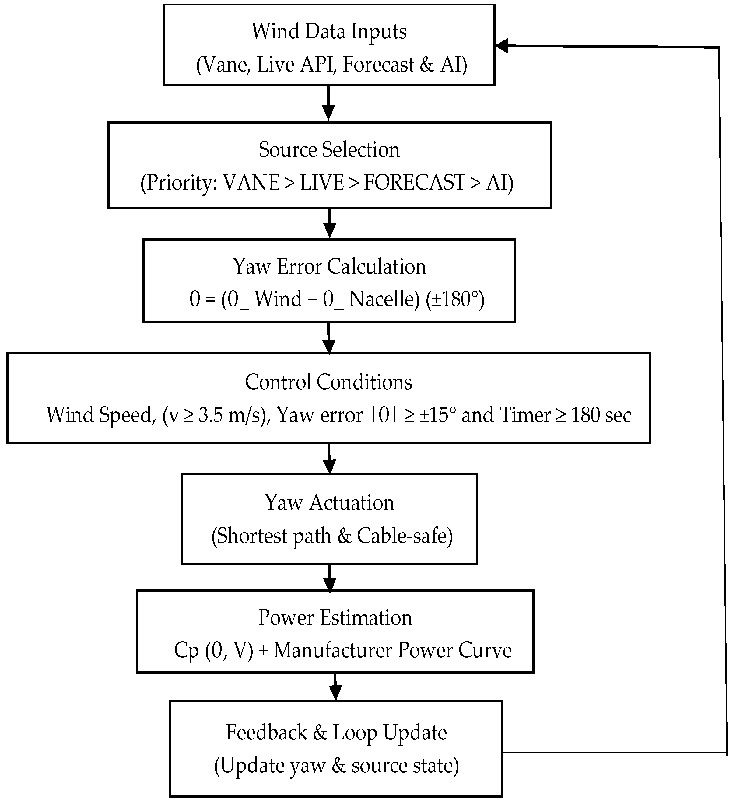
2.6. System Algorithm

Figure 6 describes the operations of the yaw control system of the wind turbine in steps. It is initiated by measuring wind speed and wind direction using a wind vane sensor and live wind data via an API. The controller then verifies that the speed of the wind has surpassed the cut-in threshold, otherwise the system stops and waits until the appropriate conditions are reached. Once the wind speed reaches a certain level, the controller compares the yaw error, and this is the difference between the orientation of the turbine nacelle and the direction the wind is blowing. This error is then assessed by the system as an equal or larger error of $\pm 15°$. When the deviation is out of this tolerance band, the yaw motor is turned on to move the nacelle in the correct direction. When the yaw error remains acceptable, the turbine maintains its current position and waits without taking any action, which can result in unwarranted movement of the motor. This minimizes wear of the mechanical components and does not allow the system to respond to short-term variations, which are not significant in influencing power production. The flowchart indicates the decision-making logic that makes the nacelle move whenever the energy gained is greater than the actuation cost. The controller ensures that the motor is not in operation when the wind is too slow to warrant movement by ensuring that the wind speed is checked before each correction. The delay functions incorporated in the loop are used to filter out the noise sensor readings and stabilize the response in windy conditions. This assessment is constantly repeated, creating a closed system that continuously provides an updated orientation with the change in the direction of the wind. Due to such a logical design, the turbine is at right angles most of the time and does not experience quick and sideways movements. The general design enhances power harvesting, shields hardware and secures similar reactions to various wind directions. Practically, this circulation assists the turbine to move effortlessly and also makes every correction during the yaw significantly add to performance.

2.7. Yaw Correction Logic Based on Wind Direction and Rotor Alignment

The Smart Wind-Tracking System in Figure 7 has a yaw mechanism that is driven by a step motor that is in turn used to check the direction that the wind is moving. The entire control logic is implemented by a microcontroller, and a magnetic encoder feeds precise information about the position of the nacelle. This closed-loop system guarantees accurate yaw positioning, minimizes yaw error, collects maximum energy and reduces mechanical forces on other parts of the system, including bearings, shafts and the gear box.

In case A, the minimum distance between the two points is calculated. Upon a change in the wind direction, the controller determines the yaw error ${(\theta }_r)$ and spins the nacelle around the shortest possible rotational track clockwise or counterclockwise, to bring it back into line with the wind. This will see that it completes the correction of the orientation fast and efficiently and reduces unnecessary motor travel.

Case B—Deadband $\pm 15°$ and 3 min Stability Timer. Here, yaw correction is only implemented in cases where the absolute yaw error is more than $\pm 15°$. When $\left|\theta r\right| \ge \pm 15°$, the controller initiates a 3 min timer to ensure that the misalignment is not temporary and that small variations do not cause misalignment. When the error equal or exceeds $15°$ in the entire 2 min, then the nacelle is turned back to the right position.

However, when the error decreases below the threshold within this interval, then the controller maintains the nacelle in the same position. The deadband-plus-timer plan eliminates unwarranted actuation, minimizes the wear of motors, and prevents constant oscillation caused by small changes in wind.

Case C—Cable Safety Limit $\left(\pm 180°\right).$ At the point where the wind direction passes over the $\pm 180°$ axis, the system will enable the cable-safe logic. Rather than rotating the same way and over-twisting the cables, the controller reverses the direction of rotation and proceeds counterclockwise to arrive at the new alignment. This makes sure that the yaw cables do not exceed the range of twisting, but at the same time, the rotor is directed properly to the wind.

2.8. Baseline Yaw Control Strategy

A traditional rule-based yaw controller is used to determine the effectiveness of the proposed strategy of yaw control. This is the kind of yaw control logic that is currently popular in small and medium wind turbines. In this scheme, the nacelle yaw angle is only calculated based on the instantaneous measurements of the wind direction without prediction, optimization, and adaptative decision-making.

The baseline controller is based on a predefined deadband of the yaw to control the yaw motion. Under the circumstances that the absolute misalignment between the nacelle’s orientation and the direction of the incoming wind is more than the given threshold, the yaw actuator is activated to reverse the alignment. On the other hand, in the event that the error in the yaw is still within the deadband, no corrective action is taken and the position of the nacelle is held constant. This method restricts unnecessary movement of the yaw axis and still allows the approximate direction of the wind to be maintained.

The baseline controller does not have any wind forecasting, artificial intelligence, multi-source data fusion, or learning-based adaptation. The current wind direction input is all that triggers all of the yaw actions. Mechanical constraints, yaw rate limits and turbine parameters are the same in order to guarantee a fair and unbiased comparison in the proposed control framework. Therefore, any difference in performance that is observable in the results can be solely accounted for due to the control strategy itself and not by the differences in system configuration or operating conditions.

The methodology described in the previous section establishes the data sources, preprocessing steps, and control strategies used to evaluate yaw control performance under realistic wind conditions. Building on this foundation, the following section presents the overall control system architecture and block diagram of the proposed yaw control framework. The control diagram illustrates how wind data, prediction modules, and control logic are integrated within the Simulink environment to generate yaw commands and evaluate system performance.

3. Control Design

Figure 8 depicts the logic of decision-making employed by the smart yaw control system in order to pick the most dependable wind direction source under different operation conditions. The flowchart is developed based on two condition priority structures aimed at maintaining continuous and fault-tolerant operation of the yaw.

This starts with reading the wind vane sensor, which is the highest priority in the source hierarchy. The controller checks the availability of the vane sensor and AI-predicted validity every 5 s. When the vane is in operation, yaw control is carried out directly with the measurements of the vane. In cases where the vane is not available because of sensor noise, hardware error, or temporary blockage, the system will jump to the live wind data source that is acquired via the OpenWeatherMap using the API key.

In the case of the live data pathway, the controller once more tests the availability of data and the validity of the related AI prediction. When the live source is on, the yaw controller will still use the real-time online measurements and watch to ensure that the vane is coming back. If the vane source and live source fail, for example, because of network breakage, the system will switch to live AI-predicted data, which also offer short-term predictions based on the most recent online dataset. This also means that the yaw alignment can still be achieved without the direct sensor or network input.

In the second scenario, where there is only one source (either vane, or live) available, the system makes use of it and falls back on its corresponding AI-predicted data in the event that the primary measurements are lost. In this fallback mode, the controller will continue checking every 5 s whether the vane or live sensor has resumed operation. Whenever a primary source becomes available again, the controller immediately switches back to it, placing AI prediction as the fallback option used only when no physical source is available.

This control diagram given in the above part outlines the general model and signal path of the proposed yaw control system. With this conceptual architecture in place, the next section describes the practical system design and implementation processes such as model development, controller setup and integration in the MATLAB Simulink R2025b environment.

4. System Design and Implementation

4.1. Hardware Implementation

All the hardware implementation details of the proposed smart yaw control system are provided in Figure 9 below, which provides the physical relationship of the major components of the system at the central microcontroller between the sensing subsystem and the actuation subsystem. The turbine structure has an analog wind vane that measures the direction of local wind, and is a continuous analog signal with a voltage range of 0–5 V, representing a full 0–360-degree wind direction. The wind vane itself operates on the 5 V of the microcontroller, and the wind direction analog output of the wind vane is hard-wired into one of the analog input pins of the controller, with the microcontroller converting the corresponding voltage into one of the wind direction angles with its internal analog-to-digital converter (ADC). On the actuation side, the microcontroller is connected to a stepper motor driver, and has three digital control signals, one being a step (PUL) signal that is used to step the driver in a direction, the other a direction (DIR) signal, which is used to turn the driver clockwise or anticlockwise, and the last being an enable (EN) signal, which is used to switch the driver off or on. These control signals are formed by the microcontroller, based on the calculated error of the yaw and the strategy that is adopted by the yaw control. This external 12 V DC power is then used to drive the motor driver, in which the required current is applied through a stepper motor that is mechanically connected to the wind turbine nacelle to make the wind turbine rotate on the yaw. It is also done through the distribution and grounding of power with the help of a breadboard that gives a common electrical reference point to all the components. Overall, it should be mentioned that the figure indicates the flow of information regarding wind sensing to control the decision-making process to future yaw actuation controlled by high-power motor circuitry with the necessary distance between low-power control electronics and high-power motor circuitry.

The components include the following:

• Microcontroller: Arduino Uno R4 WiFi (Arduino, Turin, Italy);
• Wind vane: RS-FXJT05 (Rika Sensors, Handan, China);
• Stepper motor: NEMA 17 Stepper Motor (Wantai Motor, Changzhou, China);
• Motor driver: TB6600 Stepper Motor Driver (Toshiba, Tokyo, Japan).

4.2. Software Implementation: MATLAB/Simulink Model

The offered smart yaw control system is produced in the MATLAB/Simulink environment, trying to model and establish the dynamic behavior of a horizontal-axis wind turbine under different wind conditions. Figure 10 depicts the entire Simulink architecture, which consists of four primary subsystems, namely the Wind Environment, Yaw Controller, Yaw Mode Selector and Power Output Calculation blocks. The Wind Environment subsystem is a system that takes time-varying wind speed and wind direction input based on vane, live and forecast data sources and therefore allows realistic modeling of the changing atmospheric conditions. The Yaw Controller subsystem is another closed-loop device, which reduces the yaw misalignment within a 15-degree deadband and maintains a 180-degree cable-safe rotation limit, which guarantees aerodynamic efficiency and mechanical safety. The reference model is a 3.6 kW horizontal-axis wind turbine, which is utilized to calculate the instantaneous electrical power output as a result of the existing yaw alignment and wind conditions. The Yaw Mode Selector enables the operator to change between yaw active operating mode and fixed-heading operation, so that the results of operating in controlled and uncontrolled yaw conditions may be directly compared. In the Power Output Calculation subsystem, the simulated wind speed is mapped to the generator’s electrical output using a manufacturer-derived power curve, with an additional yaw-dependent efficiency factor incorporated to realistically model power losses caused by yaw misalignment. In general, this Simulink model can be viewed as a digital representation of the wind turbine system and a stable virtual environment to test the viability of the yaw aligning process, cable safety mechanism, and the general performance of power optimization during the pre-implementation phase.

4.2.1. Wind Environment Subsystem

The subsystem below in Figure 11 represents the wind direction acquisition, validation, and AI-assisted selection logic used by the smart yaw control system. It processes wind direction inputs from three independent sources—the physical wind vane, live online data, and forecast data—each of which is conditioned using noise modeling, discrete filtering, delay blocks, and angle unwrapping to ensure continuity across the 0–360° range. Validity checks are applied to each source using threshold logic and enable switches so that unreliable or unavailable signals are automatically rejected. In parallel, an AI predictor block estimates the wind direction based on historical wind speed and direction trends when conventional sources are degraded or unavailable. A hierarchical switching mechanism then selects the most reliable wind direction signal based on predefined priority and availability conditions, while maintaining angular consistency through wrapping logic. The selected wind direction output is forwarded to the yaw controller, ensuring robust, continuous yaw reference generation under varying sensor availability and environmental conditions.

4.2.2. Yaw Controller Subsystem

Figure 12 below is the Yaw Controller subsystem, which enables the rotation of the nacelle in such a way that the turbine opens to the approaching wind and even shields the cables to ensure the smooth functioning of the motors. The system continuously takes the difference between the commanded wind direction and the feedback yaw angle and compares the yaw error at the safety limit of $\pm 180°$. A Cable-Safe Planner is utilized to ensure that the nacelle does not cross the $\pm 180°$ mechanical boundary and this eliminates the twisting of the cables when the nacelle is operated over long durations. Rate limiters and acceleration filters as well as dwell timers are also utilized by the controller and stabilize the stepper motor in such a way that yaw correction is accurate and efficient in varying wind conditions.

4.2.3. Yaw Mode Selector Subsystem

This subsystem determines the active or passive yaw control that the turbine is to pursue or if the turbine is to remain in a fixed heading. Figure 13 shows that the Yaw Mode input signal selects and the switch between the controller’s continually updated yaw command or the preset fixed position. An angle value is kept within the range of +180 to −180 and a wrap180 fixed block is utilized to allow the smoothness of the angles as they rotate and ensure that there are no sharp turns. The design makes this system flexible and enables easy comparison of fixed-yaw and active controlled operation when performing simulation and testing.

4.2.4. Power Output Calculation Subsystem

The subsystem of estimating the electrical output of the turbine in Figure 14 shows that the output depends on both the wind velocity and the orientation of the yaw. The first step it takes is to compute the error, which is the yaw, and wrap it within the range of −180 and +180. The second step is to take the error and multiply it by a cosine-cubed function, which is used to establish the proportion of the wind speed that can be effectively utilized to generate power. This fixed wind speed is entered into a look-up table and the system interpolates this with the 3.6 kW turbine power curve to obtain a real-time estimate of power.

Having the yaw control system developed and installed, the next part is to consider its behavior in the conditions of real wind. The discussion and findings are aimed at conducting a comparison of the suggested control strategy to the baseline approach, showing the improvements in the yaw alignment, power response, and the behavior of the whole system.

5. Result and Discussion

5.1. Real-Time Microcontroller Output Log

Figure 15 presents a block diagram representation derived from the Arduino serial monitor’s output, illustrating the real-time operation of the smart yaw control system and its priority-based source selection logic (VANE > LIVE > FORECAST). At system startup, the controller initializes the hardware, updates its geolocation for Mount Pearl, Newfoundland and Labrador (Canada), and establishes a Wi-Fi connection to retrieve wind information from the OpenWeatherMap service.

Under normal conditions, when all sources are available, the nacelle is aligned using the physical vane measurement (e.g., 270.5° W), resulting in a very small yaw error, typically within ±0.5°. If the Wi-Fi connection is lost, the controller continues operating in vane mode, ensuring uninterrupted yaw alignment. When the vane signal becomes unavailable but live data is restored, the controller automatically transitions to live data mode and updates the yaw position accordingly. Once the vane signal is restored, the system immediately returns to vane mode, reflecting the highest priority assigned to the physical sensor.

In scenarios where both vane and live inputs are unavailable, the controller switches to forecast mode and uses predicted wind direction data (e.g., 250° WSW) to maintain turbine alignment. The arrows in the diagram explicitly show both fallback and recovery transitions between operating modes, demonstrating continuous monitoring and automatic failover. Overall, the figure confirms that the microcontroller autonomously manages source switching, maintains stable yaw alignment, and ensures reliable operation even during temporary sensor or network interruptions.

The current arrangement of the microcontroller takes predicted wind direction data via the OpenWeatherMap API, and these predictions are usually in rough time increments (e.g., +3 h), which cannot be used in a small wind turbines to make real-time yaw adjustments. Since small turbines can have short-term variations in the wind direction, it is unwise to rely on just vane measurements or the use of forecasting information several hours old, which may result in short-term misalignment and low efficiency. In order to fill this gap, an AI-based model of short-term prediction, which is trained under MATLAB, is added to predict the wind direction within the next few minutes. This predictive capability allows the controller to respond faster and to have consistent control in sudden directional variations.

Moreover, there is a tendency of inconsistencies between the vane’s measured output of wind direction at the turbine and the live weather station data. These variations are because the station and the turbine are situated at different points and the terrain, the elevation and other local obstacles also alter the air flow. The system should have its own GPS module to remove this spatial mismatch and so that the online data are able to reflect the accurate position of the turbine. Geolocation using GPS would enable the real-time forecasting of the data to be requested at the exact coordinates of the turbine, which would enhance the directional accuracy and consistency of the yaw control process.

This research paper is discussed in two phases. First, the wind direction prediction model is trained and validated by measured wind datasets to measure the prediction accuracy. Second, the validated output of predicted values and the prediction errors is incorporated into the yaw control structure and its effect on the yaw misalignment and power generation of turbines is tested in the same wind conditions.

5.2. AI Training and Performance Evaluation Using MATLAB

This part shows the AI-based wind direction prediction model that was developed in this paper. The focus of the AI module is to help make active yaw control decisions by short-term wind direction prediction to aid long-term wind predictions. The AI model is designed as a predictive support and redundancy system in situations where there might be noise in direct wind measurements, latency in direct wind measurements or short-term unavailability. To be clear and transparent, the condition of the AI model is measured separately, and combining its results with the analysis of the yaw control and power-generation analysis will be carried out in the following sections.

Various regression-based learning methods in MATLAB were first considered when predicting the wind direction in the short term, including linear regression, support vector regression, regression tree models, and recurrent neural networks. The initial appeal of tree-based regression models is that they are easy to compute, can be interpreted, and implementation can be embedded or edge-assisted. Nevertheless, the direction of the wind is highly time dependent and circular in nature and thus constrained the usefulness of static regression models, especially during wind conditions that vary rapidly.

On these grounds, an LSTM recurrent neural network was chosen as the ultimate prediction model. The time series nature of the information required in active yaw control support suits LSTM networks well and can be used to learn short-term temporal patterns in the sequence of wind measurements, which are essential in support of active yaw control. The LSTM model is trained on inputs such as wind direction and speed that are coded in sine–cosine form so that the seam of the 0–360 boundary is continuous and so that numerical accuracy is enhanced during training.

It is necessary to underline the fact that the yaw actuator is not directly controlled by the AI model. Under the suggested system architecture, the decisions to actuate the yaw are always determined based on the real-time measurements of wind direction on the active data source, and AI prediction is also performed separately to introduce redundancy, validation, and situational awareness. This paper provides certainty and safety in yaw behavior and also provides a control framework with short-term predictive information as necessary. Consequently, the AI module improves robustness and reliability without interfering with trusted real-time measurements.

5.2.1. AI Training Workflow and Dataset Structure

The AI model was trained using real-time wind speed and wind direction data collected through a microcontroller-based system that retrieves live meteorological information from OpenWeatherMap. The dataset was sampled at 5 min intervals and contained 3665 time-synchronized samples recorded on 5 December 2025, enabling effective sequential learning for short-term wind direction prediction.

The raw angular measurements were pretrained by converting to sine–cosine representations in order to take into consideration the circular nature of wind direction. This transformation removes the artificially introduced discontinuity at the 0°/360° boundary and turns the angular data into continuous numerical characteristics that can be trained by machine learning algorithms. An example is that a wind direction of 360$°$ would be denoted as (cos = 1, sin = 0) and 20 as (cos = 0.94, sin = 0.34). This encoding also guarantees that the transition of directional changes and wrap-around transitions are learned properly by the model.

The training set is organized in the form of a sliding time window in which there are three sequential wind direction measurements, WindDirT3, WindDirT2, and WindDirT1, which denote the direction of the wind in the furthest past, the nearest past, and the nearest future, respectively. The values of each of these are represented in terms of the relevant sine–cosine pair. Another input feature of the model is wind speed, to enable the model to represent the interaction of the wind magnitude and directional change. The AI model generates the target output as WindDirT, which is the predicted direction of the wind in the coming time step, which is 5 min of the wind. During supervised training, the model learns the nonlinear temporal relationship between past wind direction states (T3 → T2 → T1), wind speed, and the future wind direction WindDirT. This formulation enables short-horizon wind direction prediction that is directly relevant for yaw control decision support.

A sample subset of the structured training data is illustrated in

Table 4. Sample of AI training dataset.

Wind Dir	Cos T3	Sin T3	Wind Dir	Cos T2	Sin	Wind Dir T1	Cos T1	Sin T1	Wind Speed	Wind Dir	Cos T	Sin T
T3			T2		T2					T
360	1	0	360	1	0	360	1	0	5.81	360	1	0
360	1	0	360	1	0	360	1	0	6.17	20	0.94	0.34
360	1	0	360	1	0	20	0.94	0.34	6.17	20	0.94	0.34
360	1	0	20	0.94	0.3	20	0.94	0.34	6.17	20	0.94	0.34
20	0.94	0.34	20	0.94	0.3	20	0.94	0.34	6.17	20	0.94	0.34
20	0.94	0.34	20	0.94	0.3	20	0.94	0.34	6.17	20	0.94	0.34
20	0.94	0.34	20	0.94	0.3	20	0.94	0.34	7.15	360	1	0
20	0.94	0.34	20	0.94	0.3	360	1	0	7.15	360	1	0
20	0.94	0.34	360	1	0	360	1	0	7.15	360	1	0
360	1	0	360	1	0	360	1	0	7.15	360	1	0

below, demonstrating how the cosine–sine encoding of the consecutive wind directions, the wind speed of that direction and the forecasted direction of the target are encoded. Through exposure to patterns such as stable wind conditions (e.g., 360° → 360° → 360°), gradual transitions (e.g., 360° → 20°), and sudden directional shifts (e.g., 20° → 360°), the model learns both steady and rapidly changing wind behaviors. The model of prediction is performed with the help of the LSTM neural network in MATLAB. The MATLAB implementation used for training the LSTM prediction model and for the real-time yaw control system is provided in the Supplementary Material (Supplementary Material S1). The network takes a sequence of input features sequentially and fills in the predicted yaw angle as a scalar value using a formulation (atan2d) that is an inverse trigonometric, which is angular consistent and avoids discontinuities. This approach ensures that the predicted yaw direction remains physically meaningful across the full 0–360° range.

Figure 16 below illustrates the prediction performance of the trained LSTM-based wind direction model using the dataset summarized in Table 4. The first subplot in Figure 16 compares the actual wind direction with the corresponding LSTM-predicted values. The close overlap between the blue solid curve (actual) and the red dashed curve (predicted) demonstrates that the model accurately tracks the temporal evolution of wind direction. Importantly, smooth transitions are observed across the 0°/360° boundary, confirming that the sine–cosine encoding and angular reconstruction effectively prevent artificial jumps in the prediction output. The second subplot shows the circular prediction error computed using an angular distance formulation. The error remains centered around 0° and is largely confined within ±10°, indicating stable and consistent short-term predictions throughout the dataset. This level of angular accuracy is well within acceptable limits for yaw control decision support, where small residual misalignment results in only marginal aerodynamic power loss. The third subplot presents the regression fit between predicted and actual yaw angles. The data points cluster closely around the fitted regression line, yielding a high correlation coefficient (R = 0.9789) and a mean squared error (MSE) of 113.32°. These results confirm a strong agreement between predicted and measured wind directions and validate the effectiveness of the LSTM-based approach for short-horizon wind direction prediction.

Taken together, the structured input data summarized in Table 4 and the performance results shown in Figure 16 indicate that the AI module successfully learned the short-term temporal evolution of wind direction (T₃ → T₂ → T₁ → T). The model’s output, WindDir_t, represents the predicted wind direction at the next time step corresponding to a 5 min prediction horizon, which is well suited for yaw control decision support. The offline evaluation using historical sequential data confirms that the LSTM-based model can accurately capture short-term wind direction dynamics and provide reliable predictions. However, while these results validate the intrinsic predictive capability of the AI model, they do not by themselves demonstrate performance when the predictor is embedded within a complete yaw control framework under real-time operating conditions, which is addressed separately through system-level simulations.

To address this, the following section evaluates the trained AI model within a closed-loop yaw control system using live wind data acquired through a microcontroller-based interface. This system-level validation examines how AI prediction interacts with real wind measurements, motor actuation, yaw error, and power output in real time. The analysis is supported by MATLAB simulation results and representative samples of live operational data, as is illustrated in Figure 16 and summarized in Table 4. It is noted that, like all data-driven models, the AI predictor performs best within the range of conditions represented in the training data. The model is therefore designed as a supportive and fallback component, rather than a sole control authority, ensuring that real-time measurements always take precedence when available.

5.2.2. AI Prediction Result and MATLAB Validation

In the validation stage, wind measurements are obtained exclusively via a microcontroller-based system using live data from the OpenWeatherMap API. The trained LSTM-based wind direction prediction model is evaluated over approximately 14 h of real-time operation. Wind speed and wind direction are retrieved continuously through a Wi-Fi connection and transmitted directly to MATLAB for processing, visualization, and control analysis. This configuration enables system-level validation of the proposed yaw control framework without reliance on local wind sensors or a physical turbine installation.

For clarity of evaluation, only the live data source is activated during this stage. This deliberate choice avoids source switching and isolates the yaw control response to real-time wind inputs. The AI model operates in parallel and generates short-term wind direction predictions; however, it does not directly actuate the yaw motor. All yaw commands are computed exclusively from live wind measurements, ensuring deterministic, safe, and physically interpretable control behavior.

Figure 17 presents the MATLAB simulation results corresponding to the operating events summarized in

Table 5. Representative samples of live wind data acquired via a microcontroller-based OpenWeatherMap API, showing AI-predicted yaw direction, motor yaw response, and yaw error used for validating the proposed yaw control system.

Time (s)	Source	Wind Dir (°)	Wind Speed	AI Predicted Yaw (°)	Motor Yaw (°)	Yaw Error (°)	Yaw Movement	Wi-Fi
1581.2	LIVE	80	3.60	5	80.0	+0.0	—(initial)	ON
1762.06	LIVE	80	3.60	5	80.0	+0.0	0.0	ON
3525.78	LIVE	293	1.79	262	293.0	−0.0	−147	ON
3526.92	LIVE	293	1.79	315	293.0	−0.0	0.0	ON
4131.01	LIVE	60	4.12	355	59.9	+0.1	+126.9	ON
4132.13	LIVE	60	4.12	5	59.9	+0.1	0.0	ON

. The subplots illustrate the interactions between wind measurements, AI prediction, yaw control, and turbine power response.

Figure 17a shows the live wind direction (wind source), the AI-predicted direction, and the motor yaw position. The wind source data are not missing; rather, they largely overlap with the motor yaw position during steady-state operation. This overlap occurs because the yaw controller successfully aligns the nacelle with the live wind direction to maximize aerodynamic efficiency. When alignment is achieved, both curves coincide, making them visually indistinguishable in certain intervals. During periods of stable wind, such as around t ≈ 1581 s and t ≈ 1762 s, the yaw motor closely tracks the live wind direction (≈80°), resulting in a yaw error near zero. Although the AI-predicted direction exhibits minor deviations, it does not directly actuate the motor. The controller prioritizes real-time live measurements for actuation while using AI prediction only for anticipatory support. When abrupt wind direction changes occur, the transient behavior becomes visible. For example, at t ≈ 3525.8 s, the wind direction shifts rapidly to approximately 293°, producing a temporary yaw error while the motor remains near its previous position. AI prediction indicates an approaching directional shift; however, the controller computes the yaw error exclusively from live measurements and commands the shortest rotation path. The motor then settles near 293°, restoring a near-zero yaw error. Similar behavior is observed at t ≈ 4131.0 s when the wind shifts to approximately 60°. These responses confirm that AI captures directional trends, while the control system ensures safe and accurate physical alignment. Figure 17b relates wind speed to both measured turbine power and predicted power output. During steady alignment, measured power follows the Falcon Silence 3.6 kW reference power curve, as shown in Figure 17c. Temporary power reductions occur during brief yaw misalignment following abrupt wind changes, which are corrected as the yaw error returns toward zero. A noticeable discrepancy between predicted and measured power is observed in certain intervals, reaching approximately 50% during rapid wind fluctuations. This deviation arises primarily from high-frequency wind speed variations present in the MATLAB simulation environment. In contrast to real-world atmospheric behavior, the simulated wind data include sharper and faster fluctuations, which amplify prediction sensitivity and result in larger instantaneous power differences. Importantly, these discrepancies occur during transitional periods rather than steady-state operation. Once wind speed stabilizes and yaw alignment is restored, predicted and measured power values converge toward the reference curve. Future implementation will incorporate improved wind filtering and adaptive prediction smoothing techniques to reduce transient prediction errors and enhance robustness under rapidly varying wind conditions. Figure 17c presents the manufacturer’s reference power curve of the Falcon Silence 3.6 kW turbine. The simulated measured power remains bounded by this curve throughout operation, confirming that the implemented aerodynamic and derating models maintain physical realism.

Figure 17d illustrates the yaw error evolution. Error spikes occur only during abrupt wind direction transitions. These spikes are short-lived and rapidly decay as the controller re-establishes alignment. During steady wind conditions, the yaw error remains near zero, confirming effective tracking performance. Figure 17e shows the turbine efficiency variation. Efficiency remains high when yaw alignment is maintained and decreases temporarily during misalignment events. Once corrective yaw action is completed, efficiency returns to near-optimal levels, demonstrating the effectiveness of the LIVE-prioritized yaw control strategy.

Table 5 below presents representative samples of live wind data used to validate the proposed AI-assisted yaw control framework. Wind speed and wind direction are acquired in real time by a microcontroller through a Wi-Fi connection to the OpenWeatherMap API and transmitted directly to MATLAB for processing. The trained LSTM model generates short-term yaw predictions, which are logged alongside the measured wind direction, motor yaw position, yaw error, and yaw movement. The yaw controller computes motor actions exclusively from the live wind measurements, while AI prediction serves as a supporting reference and does not directly actuate the nacelle. All values are reported with appropriate numerical precision consistent with measurement resolution and control accuracy. This table supports Figure 17 by illustrating how the yaw control system responds to real-time wind variations while maintaining stable alignment and minimizing unnecessary yaw movements.

Taken together, Figure 17 and Table 5 confirm that the AI prediction model functions as a supportive, non-intrusive component within the proposed yaw control architecture. The microcontroller-based live wind data serve as the sole control input, while the AI provides additional situational awareness and redundancy without overriding real-time measurements. This structure allows the system to maintain accurate alignment during rapid wind direction changes, reduce mechanical stress through shortest-path rotation, and demonstrate the feasibility of AI-assisted yaw control using online meteorological data.

The results presented in Section 5.2 demonstrate that the proposed LSTM-based AI model can reliably capture short-term wind direction dynamics and generate accurate yaw predictions under real-time operating conditions. The validation confirms that the AI module functions as a stable and supportive component within the yaw control framework, without directly influencing actuator commands when trustworthy live measurements are available. Having established the predictive accuracy and robustness of the AI model in MATLAB, the next section focuses on evaluating how this AI-assisted yaw control strategy affects turbine-level performance metrics. Section 5.3 therefore investigates the resulting yaw alignment behavior, power output, efficiency, and overall performance improvements when the validated prediction model is integrated into the complete yaw control and power-generation analysis.

5.3. Output of MATLAB/SIMULINK

5.3.1. LIVE-Based Yaw Control Performance Analysis

Figure 18 present the turbine response under LIVE-Based yaw control using real wind direction and wind speed data obtained from the Government of Canada dataset [35]. The data are plotted at 10 min intervals to clearly show the operational behavior of the turbine over time.

At t = 60 min, the wind direction (blue) and nacelle direction (brown) are aligned at approximately 15 × 10 = 150°. This alignment indicates proper yaw tracking under LIVE control. As a result, the yaw error is nearly zero, allowing efficient aerodynamic energy conversion. The power coefficient Cp is 9.99/10 = 0.99, which is close to the theoretical maximum, confirming optimal rotor alignment. The wind speed is 6.12 m/s, and accordingly, the output power is 5.08 × 100 = 508 W (0.508 kW). The moderate power level is directly related to the moderate wind speed at this time.

At t = 300 min, the wind direction is 14.02 × 10 = 140.2°, while the nacelle direction is 14.9 × 10 = 149°. The slight difference between these values indicates a small transient yaw misalignment. Consequently, the power coefficient slightly decreases to 9.23/10 = 0.923. The wind speed increases to 10 m/s, which significantly increases the available aerodynamic power. As a result, the turbine output rises to 21.95 × 100 = 2195 W (2.195 kW). The small reduction in Cp compared to t = 60 min is due to the minor yaw deviation during directional adjustment.

At t = 420 min, the wind direction and nacelle direction fully overlap at 14.10 × 10 = 141°, indicating perfect alignment. The wind speed increases further to 11.92 m/s, providing higher available wind energy. Because of this complete alignment, the power coefficient reaches 9.98/10 = 0.98, which is close to maximum aerodynamic efficiency. The turbine’s output reaches its highest observed value of 32.98 × 100 = 3298 W (3.298 kW), which is consistent with the increased wind speed and optimal yaw alignment.

At t = 510 min, the wind direction is 19.01 × 10 = 190°, while the nacelle direction is shown at −180°. This apparent negative value occurs due to the yaw angle being represented within the normalized range of −180° to +180°. When the nacelle reaches the rotational limit in one direction, the control system performs cable management (cable untwisting logic), causing the angle to wrap to −180° instead of continuing beyond +180°. This prevents excessive cable twisting inside the nacelle and maintains mechanical safety. Although the representation changes sign, the physical yaw alignment remains correct in circular angle space. At this time, wind speed decreases to 7.37 m/s, leading to a lower available aerodynamic power. The power coefficient is 9.45/10 = 0.945, slightly reduced due to transient adjustment and lower wind speed. The turbine output becomes 8.96 × 100 = 896 W (0.896 kW), which corresponds to the reduced wind speed conditions.

Overall, Figure 18 demonstrates that under LIVE yaw control, the nacelle consistently aligns with the real wind direction, maintaining high Cp values during steady conditions and restoring alignment quickly during directional changes. Power output variations directly follow wind speed variations and yaw alignment quality.

5.3.2. AI-Based Yaw Control Performance

Figure 19 presents the turbine performance when the LIVE wind source becomes unavailable and yaw alignment is maintained using the AI-based yaw prediction system. The data are shown at 10 min intervals to clearly illustrate system behavior during AI-driven operation.

At t = 60 min, the wind direction and nacelle direction coincide at approximately 17 × 10 = 170°, indicating accurate AI-based yaw alignment. Because the rotor faces the wind properly, aerodynamic efficiency is high. The power coefficient Cp equals 9.99/10 = 0.99, which is close to its optimal value. With a wind speed of 7.12 m/s, the turbine produces 8.50 × 100 = 805 W (0.805 kW). The moderate wind speed explains the moderate output power, while proper alignment explains the high Cp value.

At t = 174 min, the wind direction is 18.95 × 10 = 189.5°, while the nacelle direction is shown at −180°. This negative value results from angle normalization within the −180° to +180° range and cable management logic. Instead of rotating beyond +180°, the controller wraps the angle to −180° to prevent excessive cable twisting inside the nacelle. Although numerically different, −180° is physically equivalent to +180°, meaning alignment is maintained within circular angle space. The Cp value slightly decreases to 0.937 due to minor transient misalignment during angle transition. With wind speed at 8.77 m/s, output power rises to 1.552 kW, consistent with increased wind energy availability.

At t = 237 min, the wind direction is 170.9°, while the nacelle direction appears near +179°. This again reflects angular normalization at the rotation boundary. The controller selects the shortest rotational path while respecting cable limits. Cp reduces slightly to 0.902 due to transient adjustment. However, wind speed increases to 11.71 m/s, resulting in a significantly higher output power of 2.907 kW. The power increase is primarily driven by wind speed rather than yaw misalignment.

At t = 300 min, wind direction is 159.9°, and nacelle direction is 168.9°, indicating a small yaw deviation of approximately 9°. This minor misalignment explains the slightly reduced Cp value of 0.911. Wind speed remains high at 11.01 m/s, leading to a strong output power of 2.687 kW. The small efficiency reduction is consistent with the observed yaw offset.

At t = 420 min, wind direction and nacelle direction overlap at approximately 159°, indicating perfect alignment under AI control. Wind speed reaches 12.93 m/s, providing maximum available aerodynamic energy. Consequently, Cp increases to 0.98, and turbine output reaches its maximum observed value of 3.499 kW. This confirms that AI-based yaw control can maintain near-optimal alignment even without LIVE input.

At t = 510 min, wind direction is 210.5°, while the nacelle direction is shown as −158.3°. This representation results from angular wrapping and cable untwisting logic. In circular angle space, −158.3° is equivalent to 201.7°, which is close to the wind direction. The controller avoids excessive mechanical rotation by maintaining yaw within ±180°. Cp is 0.941, indicating good aerodynamic alignment. With wind speed reduced to 8.35 m/s, output power decreases to 1.341 kW, which is consistent with lower wind energy.

Overall, Figure 19 demonstrates that AI-based yaw control maintains stable alignment and efficient power capture even when LIVE wind measurements are unavailable. Temporary deviations are mainly due to cable management boundaries and angle normalization rather than control instability.

5.3.3. Overall Performance Comparison Between LIVE and AI-Based Yaw Control

Table 6. Comparison of LIVE-based and AI-based yaw control performance using MATLAB results.

Time (min)	Yaw Control Method	Power Output (kW)	Power Coefficient (Cp)
60	LIVE-based	0.508	0.99
60	AI-based	0.805	0.99
300	LIVE-based	2.195	0.923
300	AI-based	2.687	0.911
420	LIVE-based	3.298	0.98
420	AI-based	3.499	0.98
510	LIVE-based	0.896	0.945
510	AI-based	1.341	0.941

provides a detailed comparison of turbine performance under LIVEbased and AI-based yaw control at selected operating times (60, 300, 420, and 510 min). The results clearly indicate that the AI-based yaw control consistently achieves higher power output than the LIVEBased method under the same wind conditions.

At 60 min, both control strategies maintain excellent aerodynamic efficiency with a power coefficient (Cp) of 0.99, indicating proper alignment with the wind. However, the AI-based system produces 0.805 kW compared to 0.508 kW under LIVE control. The higher power output under AI control suggests improved alignment timing and reduced transient misalignment losses during early stage wind variation.

At 300 min, wind speed increases and both systems operate at higher power levels. The LIVE-based method generates 2.195 kW with Cp = 0.923, while the AI-based method produces 2.687 kW with Cp = 0.911. Although the Cp value for AI control is slightly lower at this instant, the overall power output is significantly higher. This indicates that the AI model likely adjusted the nacelle earlier during wind transitions, reducing the duration of yaw error and allowing more effective energy capture over the interval.

At 420 min, both methods achieve near-maximum aerodynamic efficiency with Cp = 0.98, reflecting excellent yaw alignment. Even under these optimal conditions, AI control delivers a higher output of 3.499 kW compared to 3.298 kW under LIVE control. This demonstrates that anticipatory yaw adjustments under AI control contribute to slightly improved overall energy extraction, especially during preceding wind changes.

At 510 min, wind speed decreases and overall power output drops for both systems. However, AI-based control still outperforms LIVE control, producing 1.341 kW compared to 0.896 kW. The Cp values are very close for AI (0.941) and for LIVE (0.945), indicating that the main difference in output is not due to steady-state efficiency but rather improved yaw response timing during wind direction variation.

Overall, AI-based yaw control consistently provides higher power output across all evaluated time points. The key reason for this improvement is the AI model’s ability to predict short-term wind direction trends and initiate earlier nacelle movement. This reduces the magnitude and duration of yaw misalignment, stabilizes aerodynamic performance, and enhances total energy capture compared to the purely reactive LIVE-based yaw control strategy.

5.4. Real-Time Microcontroller Output During AI Prediction Mode

Here below is the output from the microcontroller serial monitor, showing how the system behaves in AI prediction mode.

$\hspace{0.17em}$

[PRIORITY]: VANE >   LIVE    >   AI FORECAST

      [SOURCES] Snapshot (angle, speed, time)

         VANE: 264.7° (W), Time: 09- Nov 07:08:27

           LIVE: 270.0° (W), 7.2 m/s, Time: 09- Nov 07:08:27

           FCST: 319.0° (NW), 7.8 m/s, Time: 09- Nov 10:05:00      

[RUN] Motor using:    VANE 264.7° (W)

AI FORECAST Yaw (vs SRC= VANE), 294.3° (WNW) [ Δ vs src = 29.6°]

Motor pos:  264.7° (W) | Error: 0.0°

[STATUS] VANE = OK | LIVE = OK | Forecast = OK || Wi-Fi = OK |Counts V/L/F =    2/2/0 | Wi-Fi reconnects = 0| Motor Pos = 264.7°| Err = 0.0°

$\hspace{0.17em}$

[PRIORITY]: VANE    >   LIVE    >   FORECAST

      [SOURCES] Snapshot (angle, speed, time)

          VANE: (lost)

           LIVE: (lost)

           FCST: 319.0° (NW), 7.8 m/s, Time: 09- Nov 10:05:00

[RUN] Motor using:    AI Predicted 294.3° (WNW)

AI FORECAST Yaw (vs SRC= VANE), 294.3° (WNW) [ Δ vs src = 0°]

Motor pos:  294.3° (W) | Error: 0.0°

[STATUS] VANE = LOST | LIVE = LOST | Forecast = OK || Wi-Fi = LOST |Counts V/L/F = 2/2/0 | Wi-Fi reconnects = 0| Motor Pos = 294.3°| Err = 0.0°

$\hspace{0.17em}$

[PRIORITY]: VANE    >   LIVE    >   FORECAST

[SOURCES] Snapshot (angle, speed, time)

      VANE: (lost)

      LIVE: 270.0° (W), 7.2 m/s, Time: 09- Nov 07:16:35

     FCST: 319.0° (NW), 7.8 m/s, Time: 09- Nov 10:05:00

[RUN] Motor using:    LIVE 270.0° (W)

AI Predicted Yaw (vs SRC  LIVE, speed= 7.2 m/s from LIVE Time: 09- Nov 07:23:35): 299.5° (WNW) [ Δ vs src = 29.5°]

Motor pos:  270.0° (W) | Error: 0.0

[STATUS] VANE = LOST | LIVE = OK | Forecast = OK || Wi-Fi = OK |Counts V/L/F=2/2/0 | Wi-Fi reconnects= 0| Motor Pos=270.0° | Err= 0.0°

$\hspace{0.17em}$

[PRIORITY]: VANE >   LIVE    >   FORECAST

[SOURCES] Snapshot (angle, speed, time)

     VANE: (lost)

      LIVE: (lost)

      FCST: 319.0° (NW), 7.8 m/s, Time: 09- Nov 10:05:00

[RUN] Motor using:    AI Predicted 299.5° (WNW)

AI Predicted Yaw (vs SRC=LIVE, speed= 7.2 m/s from LIVE Time: 09- Nov 07:29:03): 299.5° (WNW) [ Δ vs src = 0°]

Motor pos:  299.5° (W) | Error: 0.0°

[STATUS] VANE = LOST | LIVE = LOST | Forecast = OK || Wi-Fi = OK |Counts V/L/F=2/2/0 | Wi-Fi reconnects= 0| Motor Pos = 299.5°| Err= 0.0°

$\hspace{0.17em}$

Although the findings provided in the last part indicate the technical efficiency of the offered yaw control approach and AI-based prediction model, practical implementation is also limited by economic considerations. Thus, the section below will assess cost implications of the proposed system, including hardware elements, implementation needs, and general cost-effectiveness of the proposed system in small-sized wind tur-bine applications.

5.5. Scalability of the Proposed Yaw Control System for Large-Scale Wind Turbines

Although the experimental validation was conducted on a low-power laboratory-scale wind turbine platform due to facility limitations, the proposed AI-based yaw control strategy is inherently scalable to large-capacity wind turbines (e.g., 10 MW–15 MW systems). The developed control algorithm operates independently of turbine-rated power and primarily depends on wind direction sensing, yaw position feedback, and actuator control logic.

In large-scale commercial wind turbines, such as 10 MW or 15 MW units, the yaw mechanism typically employs high torque electric yaw drives and multiple geared motors instead of stepper motors used in laboratory validation. However, the control architecture remains fundamentally similar, consisting of wind direction sensors, nacelle position encoders, and a supervisory controller. Therefore, the proposed intelligent yaw alignment algorithm can be directly implemented in industrial-scale systems by integrating it into existing turbine control units (TCUs) without modification of the core control logic.

The primary difference between small-scale and large-scale implementation lies in actuator torque capacity and structural loading requirements, rather than in the control strategy itself. Since the algorithm processes the wind misalignment angle and generates corrective yaw commands independent of turbine size, the methodology remains applicable to multi-megawatt offshore and onshore wind turbines.

6. Cost–Benefit Analysis

The use of AI together with live online weather data gives the proposed yaw control system clear advantages in both cost and reliability compared with traditional sensor-based designs. Conventional systems depend on mechanical wind vanes and transmitter–receiver units to measure and send wind direction signals. These devices add to the overall hardware cost, need periodic calibration, and are often affected by wear, corrosion, or signal faults in harsh outdoor conditions. In this research work, the AI model and the live weather data replace the physical wind vane and the associated communication hardware. Real-time wind direction and speed are taken directly from reliable online weather sources, which reduces the amount of equipment required and simplifies the entire system. This lowers installation costs and reduces long-term maintenance demands. In addition, the control logic drives the yaw motor only when the deviation from the wind direction becomes larger than ±15°, so unnecessary movements are avoided and the motor experiences less mechanical stress, helping it last longer.

Comparative Cost–Benefit Summary

Table 7. Comparative cost–benefit analysis of conventional and AI-based smart yaw control systems.

Aspect	Conventional System	AI-Based Smart System	Benefit/Savings
Wind Direction Input	Physical wind vane sensor	Online live wind data via AI	Eliminates sensor cost
Data Communication	Transmitter–receiver modules	Cloud-based online data	Removes hardware modules
Yaw Motor Operation	Continuous adjustments	Threshold-based activation	Lower Motor stress, longer lifespan
GPS-Assisted Location	Not available	GPS used to obtain nearest weather-station data	Higher directional accuracy, improved power capture
Power Capture Efficiency	90–95%	98–99%	3–5% higher power generation
Energy Use for Yaw	High	Low	10–15% energy saving
Maintenance Frequency	Regular servicing	Minimal maintenance	30–40% maintenance cost

below is a clear comparison between a traditional yaw control system and the proposed AI-based smart solution, which demonstrates improvements in functionality and total cost. The traditional design relies on physical wind vane sensors and transmitter–receiver units, which add to the cost of installation and require regular maintenance. These elements also impose an additional burden on the yaw mechanism, as the motor is forced to respond to frequent changes in the wind direction and, as a result, it runs almost continuously. Conversely, the AI-based system relies on real-time online wind information, short-term projection, and location selection through GPS to receive the correct directional information from the closest weather station. This saves the use of several hardware components, decreases the maintenance of sensors, and enhances accuracy in alignment, particularly in cases where the wind conditions vary rapidly. Two foundations are used to obtain the numerical values: the first one is the aerodynamic yaw misalignment theory of power retention and the second one is a relative index model of yaw actuation energy and maintenance cost. First, the effective power capture due to yaw alignment is evaluated using the standard cosine-cubed relationship P ($\theta$) = $P_0{cos}^3\theta$, where $P_0$ is power at perfect alignment and $\theta$ is the yaw error. Conventional yaw systems typically allow persistent yaw errors in the range of 10–15° because reactive control and practical deadbands avoid constant actuation; this corresponds to ${cos}^3\left(10°\right)=0.955 (95.5\%)$ and ${cos}^3\left(15°\right)=0.901 (90.1\%)$. Therefore, Table 6 reports 90–95% retained aerodynamic power. The proposed controller achieves a smaller yaw error during sustained wind direction trends because it combines multi-source data (vane + online data) with AI prediction as a fallback during data interruptions. For $\theta \le 5°,{cos}^3\left(5°\right)=0.989 (98.9\%)$; therefore, Table 6 shows 98–99% retained aerodynamic power. Importantly, the controller does not chase every small fluctuation, which would increase gearbox and bearing stress; yaw actuation is limited using the deadband (typically ±10–15°), dwell-time, filtered wind direction, and rate-limited yaw commands. Second, yaw actuation energy is estimated using yaw activity as an energy proxy because, for the same actuator and supply conditions, energy scales with total movement/actuation time; thus, yaw energy saving is computed as ${\displaystyle \frac{A_{conv}-A_{AI}}{A_{AI}}}\ast 100$, where A is cumulative yaw motion (sum of absolute step counts or yaw angle changes). With deadband and dwell-time, the proposed controller reduces yaw activity by approximately 10–15%, which is reported as the yaw energy-saving range. Finally, maintenance cost reduction is derived from a normalized maintenance index that separates maintenance into hardware servicing and yaw wear servicing, $C_{maint}=C_{HW}+ C_{yaw}$, with the conventional system normalized to 1.0. Because exposed electrical/communication hardware and wiring represent a major portion of servicing effort in small yaw systems, conservative weighting is applied $(C_{HW,conv}=0.60$, $C_{yaw,conv}=0.40)$. Since the transmitter–receiver modules are fully removed while the vane remains, hardware-related maintenance, ${\Upsilon }_{HW}$, is conservatively reduced by 35–50%, and wear-related maintenance, ${\Upsilon }_{yaw}$, is reduced by 15–20% due to fewer yaw actions; applying these reductions gives $C_{maint,AI}=0.60 \left(1-{\Upsilon }_{HW}\right)+0.40 (1- {\Upsilon }_{yaw})$, which results in an overall reduction of approximately 27–38% and is reported as a conservative rounded range of 30–40% to account for deployment variability.

7. Limitations and Future Directions

The present system uses a physical wind vane for real-time yaw measurement and an AI model trained on both on-site sensor data and live online wind direction information. This combined structure helps the turbine operate continuously, because the controller can shift between the vane, online weather data, and AI prediction whenever one source becomes unavailable. Since the AI model learns from both types of inputs, it can estimate short-term wind direction when the vane becomes unstable or when online updates are slow. Even with these strengths, the system still has some limitations. The online weather data comes from nearby meteorological stations rather than the exact turbine location, so small differences between the station readings and the actual on-site wind field may appear. These differences become more noticeable when both the vane and the live online data are unavailable and the controller must rely only on AI prediction. In such cases, the AI has no fresh input to correct itself, and its estimates may be less accurate. Adding GPS would allow the system to automatically choose the nearest weather station and improve alignment accuracy and power capture.

The mechanical wind vane also introduces limitations. There are many factors such as exposure to dust, moisture, temperature changes, and corrosion that can affect its moving parts and reduce sensitivity, which may cause slow or uneven responses. At low wind speeds, the vane may not align properly because of inertia, and this can lead to unstable readings. Calibration drift, electrical noise, and the use of a single measurement point further reduce accuracy, especially in turbulent areas or complex terrain. Severe gusts or storms can even damage the vane or cause temporary data loss, which would require maintenance or recalibration.

The system also depends on a stable internet connection for live data updates, and the current AI model—although trained on both sensor and weather station data—uses a fixed training set and does not update itself automatically during operation. Future work will focus on GPS-assisted selection of weather stations, adaptive AI models that can learn from ongoing turbine performance, and a stronger hybrid-sensing approach that combines vane feedback with short-term prediction to keep the system reliable during network outages. Expanding the design for larger turbines, testing it at different locations, and adding faster onboard processing will help improve yaw response, mechanical protection, and long-term performance.

8. Concluding Remarks

The smart yaw control system developed in this study demonstrates that real-time sensing, intelligent control, and data-driven prediction can be effectively integrated to enhance wind turbine performance. The proposed framework combines a physical wind vane sensor with an AI-based predictive model trained on live meteorological data, enabling continuous nacelle alignment with changing wind direction. This coordinated approach significantly reduces yaw misalignment, minimizes unnecessary motor actuation, and decreases mechanical wear and associated power losses.

Both simulation and hardware validation results confirm that the AI-supported controller maintains yaw deviation within ±15°, ensuring stable turbine operation and power output close to the rated capacity. The implementation of a multi-source priority control strategy further enhances system reliability by allowing uninterrupted operation in the event of sensor malfunction or communication failure. Additionally, the optimized control logic limits excessive yaw motor movement, thereby extending mechanical component lifespan and reducing maintenance requirements.

Although experimental validation was conducted on a laboratory-scale prototype due to facility limitations, the proposed yaw control architecture is inherently scalable to large-capacity wind turbines (e.g., 10–15 MW systems). The control algorithm operates independently of turbine-rated power and can be integrated into industrial yaw drive systems with appropriately sized actuators and torque mechanisms. Therefore, the methodology is applicable not only to small and medium wind turbines but also to utility-scale and offshore wind energy systems.

Future enhancements, including GPS-based weather station selection, adaptive AI retraining mechanisms, and advanced sensor fusion techniques, could further improve alignment accuracy, system robustness, and overall energy capture in next-generation wind energy installations.

References

1. Global Wind Energy Council. Global Wind Report 2024; GWEC: Brussels, Belgium, 2024; Available online: https://www.gwec.net/hubfs/Website-2023/documents/GWEC-2024.pdf?hsLang=en (accessed on 3 September 2025).
2. Burton, T.; Jenkins, N.; Sharpe, D.; Bossanyi, E. Wind Energy Handbook, 3rd ed.; John Wiley & Sons: Chichester, UK, 2021; pp. 17–21. [Google Scholar]
3. Burton, T.; Sharpe, D.; Jenkins, N.; Bossanyi, E. Wind Energy Handbook, 2nd ed.; Wiley: Chichester, UK, 2011; pp. 97–98. [Google Scholar]
4. Liew, J.Y.; Urbán, A.M.; Andersen, S.J. Analytical Model for the Power–Yaw Sensitivity of Wind Turbines Operating in Full Wake. Wind Energy Sci. 2020, 5, 427–437. [Google Scholar] [CrossRef]
5. Wang, Y.; Liu, Z. Fatigue Analysis of Wind Turbine and Load Reduction through Wind-Farm-Level Yaw Control. Energy 2025, 326, 136266. [Google Scholar] [CrossRef]
6. Gao, L.; Li, H.; Wang, J.; Yang, C. Data-Driven Yaw Misalignment Correction for Wind Turbines. Energies 2021, 14, 3481. Available online: https://arxiv.org/pdf/2109.08998 (accessed on 3 September 2025).
7. Astolfi, D.; Pandit, R.; Lombardi, A.; Terzi, L. Diagnosis of Wind Turbine Systematic Yaw Error through Nacelle Anemometer Measurement Analysis. Sustain. Energy Grids Netw. 2023, 34, 101071. [Google Scholar] [CrossRef]
8. Pei, Y.; Qian, Z.; Jing, B.; Kang, D.; Zhang, L. Data-Driven Method for Wind Turbine Yaw Angle Sensor Zero-Point Shifting Fault Detection. Energies 2018, 11, 553. [Google Scholar] [CrossRef]
9. Mittelmeier, N.; Kühn, M. Determination of optimal wind turbine alignment into the wind and detection of alignment changes with SCADA data. Wind Energy Sci. 2018, 3, 395–408. Available online: https://wes.copernicus.org/articles/3/395/2018/ (accessed on 4 September 2025). [CrossRef]
10. Liu, Y.; Liu, S.; Zhang, L.; Cao, F.; Wang, L. Optimization of the Yaw Control Error of Wind Turbine. Front. Energy Res. 2021, 9, 626681. Available online: https://www.frontiersin.org/articles/10.3389/fenrg.2021.626681/pdf (accessed on 7 September 2025). [CrossRef]
11. Saenz-Aguirre, A.; Zulueta, E.; Fernandez-Gamiz, U.; Ramos-Hernanz, J.A.; Lopez-Guede, J.M. Self-Tuning Yaw Control Strategy of a Horizontal-Axis Wind Turbine Based on Machine Learning. In Numerical Methods for Energy Applications; Mahdavi Tabatabaei, N., Bizon, N., Eds.; Springer: Cham, Switzerland, 2021; pp. 879–900. [Google Scholar] [CrossRef]
12. Bu, F.; Huang, W.; Hu, Y.; Xu, Y.; Shi, K.; Wang, Q. Study and Implementation of a Control Algorithm for Wind Turbine Yaw Control System. In Proceedings of the IEEE Canada Electrical Power Conference (EPC), Montreal, QC, Canada, 26–28 October 2009; pp. 1–7. [Google Scholar] [CrossRef]
13. Kadoche, E.; Gourvénec, S.; Pallud, M.; Levent, T. Multi-Agent Reinforcement Learning for Wind Farm Yaw Control. Energies 2023, 16, 7892. [Google Scholar] [CrossRef]
14. Puech, A.; Read, J. Reinforcement Learning for Optimal Single-Turbine Yaw Control. Energies 2023, 16, 4521. Available online: https://arxiv.org/pdf/2305.01299 (accessed on 12 September 2025).
15. Al-Rubaye, S.Z.; Gil-Pita, R. A Novel Optimization Method for Maximizing Wind Farm Performance through Turbine Positioning and Yaw Angle Estimation. Energy Convers. Manag. 2026, 347, 120546. [Google Scholar] [CrossRef]
16. Anagnostopoulos, S.; Bauer, J.; Clare, M.C.A.; Piggott, M.D. Multi-Fidelity ML Models for Real-Time Active Yaw Control in Wind Farms. Energies 2023, 16, 6124. Available online: https://arxiv.org/pdf/2303.16274 (accessed on 8 September 2025).
17. Yang, J.; Liu, Y.; Zhang, Z.; Ma, Z.; Wang, Y. Review of Control Strategy of Large Horizontal-Axis Wind Turbines Yaw System. Wind Energy 2021, 24, 97–115. [Google Scholar] [CrossRef]
18. Wu, Z.; Wang, H. Research on Active Yaw Mechanism of Small Wind Turbines. Energy Procedia 2012, 16, 53–57. [Google Scholar] [CrossRef][Green Version]
19. Islam, M.; Biswas, P.; Rahman, M.; Rahman, A.; Hossain, M. An Intelligent Wind Turbine with Yaw Mechanism Using Machine Learning to Reduce High-Cost Sensors Quantity. ResearchGate Preprint. 2023. Available online: https://ijeecs.iaescore.com/index.php/IJEECS/article/view/29384 (accessed on 24 February 2026).
20. Joshi, A.Y.; Soni, S.G. Design of Active Yaw Control Mechanism for Small Horizontal Axis Wind Turbines. Int. J. Res. Sci. Innov. 2015, 2, 47–49. Available online: https://rsisinternational.org/Issue11/47-49.pdf (accessed on 9 September 2025).
21. Kerling, I.M.; Zimmer, D. A Yaw Control Approach Using Economic Aspects. In Proceedings of the 5th International Conference on Contemporary Problems of Thermal Engineering (CPOTE 2018), Gliwice, Poland, 18–21 September 2018; Institute of Thermal Technology: Gliwice, Poland, 2018; Available online: https://elib.dlr.de/123975/1/CPOTE2018_final_kerling.pdf (accessed on 18 September 2025).
22. Tsioumas, E.; Karakasis, N.; Jabbour, N.; Mademlis, C. Indirect Estimation of the Yaw-Angle Misalignment in a Horizontal Axis Wind Turbine. In Proceedings of the 2017 IEEE 26th International Symposium on Industrial Electronics (ISIE), Edmonton, AB, Canada, 21–23 June 2017; pp. 1239–1246. [Google Scholar] [CrossRef]
23. Shahadat, M.M.Z.; Chaity, T.T.; Ahmed, M.M.; Kader, M.I.; Snigdho, N.A. Enhancing the Wind Energy Harvesting Capacity of a Horizontal Axis Wind Turbine (HAWT) Using a Novel Wind Tracking System. In Proceedings of the IEEE International Conference on Power, Electrical, Electronics and Industrial Applications (PEEIACON 2024), Rajshahi, Bangladesh, 12–13 September 2024; pp. 1–6. [Google Scholar] [CrossRef]
24. Abhi, S.B.; Hossain, M.I.; Hoque Suny, R.; Zahura, F.T.; Hazari, M.R.; Jahan, E.; Mannan, M.A. Design and Implementation of a Smart Wind Turbine with Yaw Mechanism. In Proceedings of the 3rd International Conference on Robotics, Electrical and Signal Processing Techniques (ICREST 2023), Dhaka, Bangladesh, 7–8 January 2023; pp. 358–362. [Google Scholar] [CrossRef]
25. Yin, X.; Zhao, X. LSTM Predictive Yaw Control for Offshore Wind Turbines. Energies 2021, 14, 6301. [Google Scholar]
26. Yang, Y.; Solomin, E.V.; Shishkov, A.N. Wind Direction Prediction Based on Nonlinear Autoregression and Elman Neural Networks for the Wind Turbine Yaw System. Preprint, SSRN 4128942. 2022. Available online: http://dx.doi.org/10.2139/ssrn.4128942 (accessed on 1 February 2026).
27. Rott, A.; Höning, L.; Hulsman, P.; Lukassen, L.J.; Moldenhauer, C.; Kühn, M. Wind Vane Correction During Yaw Misalignment for Horizontal-Axis Wind Turbines. Wind Energy Sci. 2023, 8, 1755–1770. [Google Scholar] [CrossRef]
28. Santoni, C.; Zhang, Z.; Sotiropoulos, F.; Khosronejad, A. A Data-Driven Machine Learning Approach for Yaw Control Applications of Wind Farms. Theor. Appl. Mech. Lett. 2023, 13, 100471. [Google Scholar] [CrossRef]
29. Elkodama, A.; Abdellatif, A.; Shaaban, S.; Rushdi, M.A.; Yoshida, S.; Ismaiel, A. Investigation into the Yaw Control of a Twin-Rotor 10 MW Wind Turbine. Appl. Sci. 2024, 14, 9810. [Google Scholar] [CrossRef]
30. IEC 61400-1:2019; Wind Energy Generation Systems–Part 1: Design Requirements. International Electrotechnical Commission: Geneva, Switzerland, 2019.
31. Falcon Silence 3.6 kW Wind Turbine. Turbinawiatrowa. Available online: https://www.turbinawiatrowa.com/EN-H4/oferta/3/turbina-wiatrowa-36kw-falcon-silence.html (accessed on 5 January 2026).
32. Hansen, M.O.L. Aerodynamics of Wind Turbines, 3rd ed.; Routledge: New York, NY, USA, 2015; pp. 21–24. [Google Scholar]
33. Sereema. Yaw Misalignment: (R)Evolution; Technical White Paper; Sereema SAS: Montpellier, France, 2019; p. 11. Available online: https://www.sereema.com/documents/yaw-misalignment-white-paper (accessed on 17 November 2025).
34. Historical and Live Weather Data for Paradise, Newfoundland and Labrador (City ID: 6324733). Available online: https://openweathermap.org/city/5905393 (accessed on 12 January 2026).
35. Environment and Climate Change Canada. Historical Climate Data—Search and Download. Government of Canada. 2024. Available online: https://climate.weather.gc.ca/historical_data/search_historic_data_e.html (accessed on 10 January 2026).
Figure 1. Workflow diagram of the proposed AI-based yaw control system.
Processes 14 01084 g001
Figure 2. Real wind turbine used for experimental testing at Bonavista, NL.
Processes 14 01084 g002
Figure 3. Yaw- and wind speed-dependent aerodynamic power derating factor.
Processes 14 01084 g003
Figure 4. Power curve of the reference turbine.
Processes 14 01084 g004
Figure 5. Block diagram of the proposed smart wind turbine system. Arrows indicate the direction of power and control signal flow. The dashed box represents the yaw control subsystem. Standard electrical symbols denote the rectifier, inverter, DC source, and associated components.
Processes 14 01084 g005
Figure 6. Flowchart of real-time yaw control algorithm.
Processes 14 01084 g006
Figure 7. Yaw control strategy based on wind direction. The blue arrows and dashed lines indicate the incoming wind direction used to determine the nacelle yaw adjustment.
Processes 14 01084 g007
Figure 8. Priority-based yaw control logic for wind turbine alignment.
Processes 14 01084 g008
Figure 9. Connection diagram of hardware setup.
Processes 14 01084 g009
Figure 10. MATLAB/Simulink-based design for dynamic yaw alignment and power output.
Processes 14 01084 g010
Figure 11. Wind Environment subsystem in MATLAB/Simulink showing the priority-based selection of vane, live, and forecast wind inputs. The circled numbers denote signal port identifiers used for internal routing in the Simulink model.
Processes 14 01084 g011
Figure 12. Yaw Controller subsystem for nacelle alignment and cable-safe operation.
Processes 14 01084 g012
Figure 13. Mode selection logic for enabling or disabling active yaw control.
Processes 14 01084 g013
Figure 14. Power and yaw error calculation model.
Processes 14 01084 g014
Figure 15. Microcontroller output of smart yaw control source selection and fallback logic.
Processes 14 01084 g015
Figure 16. Performance of the trained LSTM-based wind direction prediction model showing (a) actual vs predicted yaw direction, (b) circular prediction error, and (c) regression fit between predicted and actual yaw angles (R = 0.9789, MSE = 113.32°).
Processes 14 01084 g016
Figure 17. MATLAB simulation results of the AI-assisted yaw control system, showing (a) yaw position tracking with live wind direction, AI prediction, and motor position; (b) wind speed and corresponding measured and predicted turbine power versus time; (c) Falcon Silence 3.6 kW reference power curve; (d) yaw error dynamics; and (e) turbine efficiency variation during operation.
Processes 14 01084 g017
Figure 18. Turbine performance under live yaw control using 10-min interval data, showing output power, power coefficient (Cp), wind direction, nacelle direction, and wind speed. For visualization on a common axis, scaling factors are applied: power (W/100), Cp (×10), and wind/nacelle direction (°/10). Yaw angles are plotted in the −180° to +180° range for clarity.
Processes 14 01084 g018
Figure 19. Turbine response under AI-based yaw control using 10-min interval data, showing turbine output power, power coefficient (Cp), wind direction, nacelle direction, and wind speed. For visualization on a common axis, scaling factors are applied: power (W/100), Cp (×10), and wind/nacelle direction (°/10). Yaw angles are represented in the normalized range of −180° to +180°.
Processes 14 01084 g019