Mathematical Modeling of Microbial Hydrocarbon Degradation Using Analytical and Runge–Kutta Methods

Abstract

Petroleum hydrocarbons remain major environmental contaminants, and understanding the mechanisms governing their biodegradation is essential for designing effective remediation plans. The strategy in this article is slightly different from other cases in the literature. Such literature models require, for their elaboration, a significant number of experiments; the number of experimental determinations is at least proportional to the square of the number of constants introduced in the mathematical expressions. For this reason, the strategy followed in this article is different—starting from a set of experiments carried out and presented in a coherent and published manner, a simple methodology for building specific and minimal models, which will allow solving specific problems, was effectively developed. This study develops a nonlinear mathematical structure, expressed as a system of coupled differential equations, that simultaneously describes the degradation of petroleum hydrocarbons and the dynamics of hydrocarbon-degrading bacteria and fungi in soil–sludge mixtures. The model was calibrated using experimental data obtained from biopiles prepared with different volumetric ratios of contaminated soil and sewage sludge. Approximate analytical solutions were derived and the distributed constants were evaluated. For a consistent discussion, the analytical solutions were assessed against numerical desk simulations performed with a classical fourth-order Runge–Kutta method, which accurately reproduced the nonlinear behavior of the specific system. This numerical approach was chosen in order to overcome the proper difficulties encountered in this strategy implementation. The results show that the soil–sludge ratio strongly influences biodegradation efficiency, while kinetic parameters determine whether microbial communities evolve toward a stationary regime or accelerated contaminant removal. The combined analytical–numerical framework provides a robust predictive tool for optimizing mixture composition and improving the design of bioremediation treatments for petroleum-contaminated soils.

1. Introduction

Soil contamination with petroleum hydrocarbons remains one of the most persistent and complex environmental challenges, affecting the physical, chemical, and microbiological properties of soils and the functioning of natural ecosystems. Activities within the petroleum industry—from extraction and transport to storage—generate long-lasting contamination that reduces soil fertility and promotes the migration of pollutants toward groundwater. Petroleum hydrocarbons form a complex mixture of aliphatic and aromatic compounds whose chemical structure influences their mobility and degradability in terrestrial environments.

In historically contaminated sites, such as the one analyzed in this study, pollution results from repeated spills associated with long-term operational activities, generating mixtures of hydrocarbons with varying degrees of volatility and biodegradability. Such soils lose their functionality and can be reintegrated into natural or economic systems only after the implementation of adequate remediation measures.

Bioremediation has emerged as a reference technology due to the ability of microorganisms to transform organic pollutants into non-hazardous end products, while the efficiency of the process depends on factors such as nutrient availability, contaminant concentration, moisture, and the structure of microbial communities. In this context, sewage sludge represents a valuable resource due to its high content of organic matter, nutrients, and active microorganisms, and has been successfully used in bioremediation processes.

The experimental foundation of this study is based on data published in a previous article [1], published in Processes, which provided detailed measurements on the evolution of petroleum hydrocarbon concentrations and the dynamics of hydrocarbon-degrading bacteria and fungi in soil–sludge mixtures. In this study, the experimental data are used exclusively as input for the development of the mathematical model. These data enable the formulation of a coherent and robust predictive model, capable of capturing the essential mechanisms of bioremediation and supporting process optimization under real field conditions.

From an applied perspective, the critical parameter in current remediation practices is treatment time, and process optimization depends on determining the concentration of microorganisms required to achieve the desired degradation in the shortest possible time. In practice, determining initial microorganism concentrations in large volumes of sludge is difficult and costly, which justifies the use of a numerical approach [2,3,4].

Two optimization approaches are possible:

(1) Estimating the initial concentration of microorganisms relative to the volume or mass of contaminated soil, based on an experimental algorithm [5,6,7].

(2) Using soil–sludge mixing ratios and determining the optimum through a mathematical model [8,9,10].

The strategy in this article is slightly different from other cases in the literature. Currently, there is a wide range of proposed mathematical models, with an increasingly high complexity and with disparate sets of constants. Such proposed models require, for their elaboration, a significant number of experiments, the number of experimental determinations being at least proportional to the square of the number of constants introduced in the mathematical expressions.

On the other hand, a wide range of different structures regarding mathematical expressions is observed, being used both simple analytical expressions, which can ensure an interpolation of different cases, and combinations of functions that are quite difficult to explain naturally, in the context of a biological process. In this case, complex mathematical models, with nonlinear expressions, with a number of eight or even 10 distributed constants, require a large number of experimental determinations and also different experimental configurations, which can be quite time-consuming and expensive.

For this reason, the strategy followed in this article is different—starting from a set of experiments carried out and presented in a coherent and published manner, we can develop a simple methodology for building specific models, which will allow solving specific problems effectively. In this sense, we present such an approach, starting from a set of experiments carried out, presented, and published in the literature. Based on them, we can develop a semi-empirical model based on results from the literature. The requirement pursued is to build efficient analytical solutions, with a minimal number of distributed constants, for an optimal cost of solving the problem. In the last section, in order to be able to analyze the solutions obtained, we presented a solution based on a numerical approach. For this purpose, a classical fourth–order Runge–Kutta integration method was chosen, the used script being described in the Results section. This method was chosen in order to use the same integration step for all three state quantities considered, and to be able to highlight any difficulties in approaching such a numerical procedure, and to be able to make comparisons more easily.

For a consistent discussion, the analytical solutions were assessed against numerical desk simulations performed with a classical fourth-order Runge–Kutta method, in order to succeed in accurately reproducing the nonlinear behavior of the specific system. This numerical approach was chosen in order to overcome the proper difficulties encountered in this strategy implementation. The script presented was implemented in MAPLE and this approach was chosen in order to emphasize all the implementation difficulties for this strategy. It was appealed to the natural freedom to choose the simplest and most direct way of implementing the solutions, in order to be able to observe the eventual difficulties. In this sense, it avoided the predefined procedures from the various predefined packages.

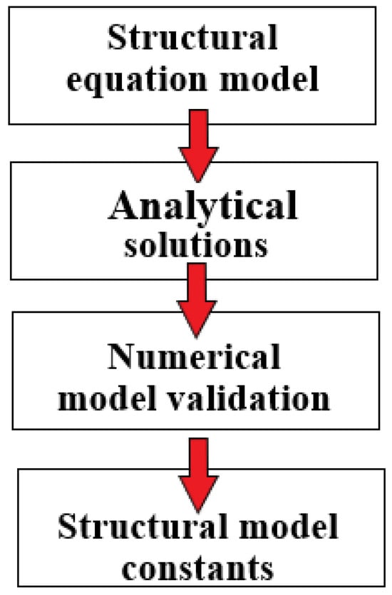
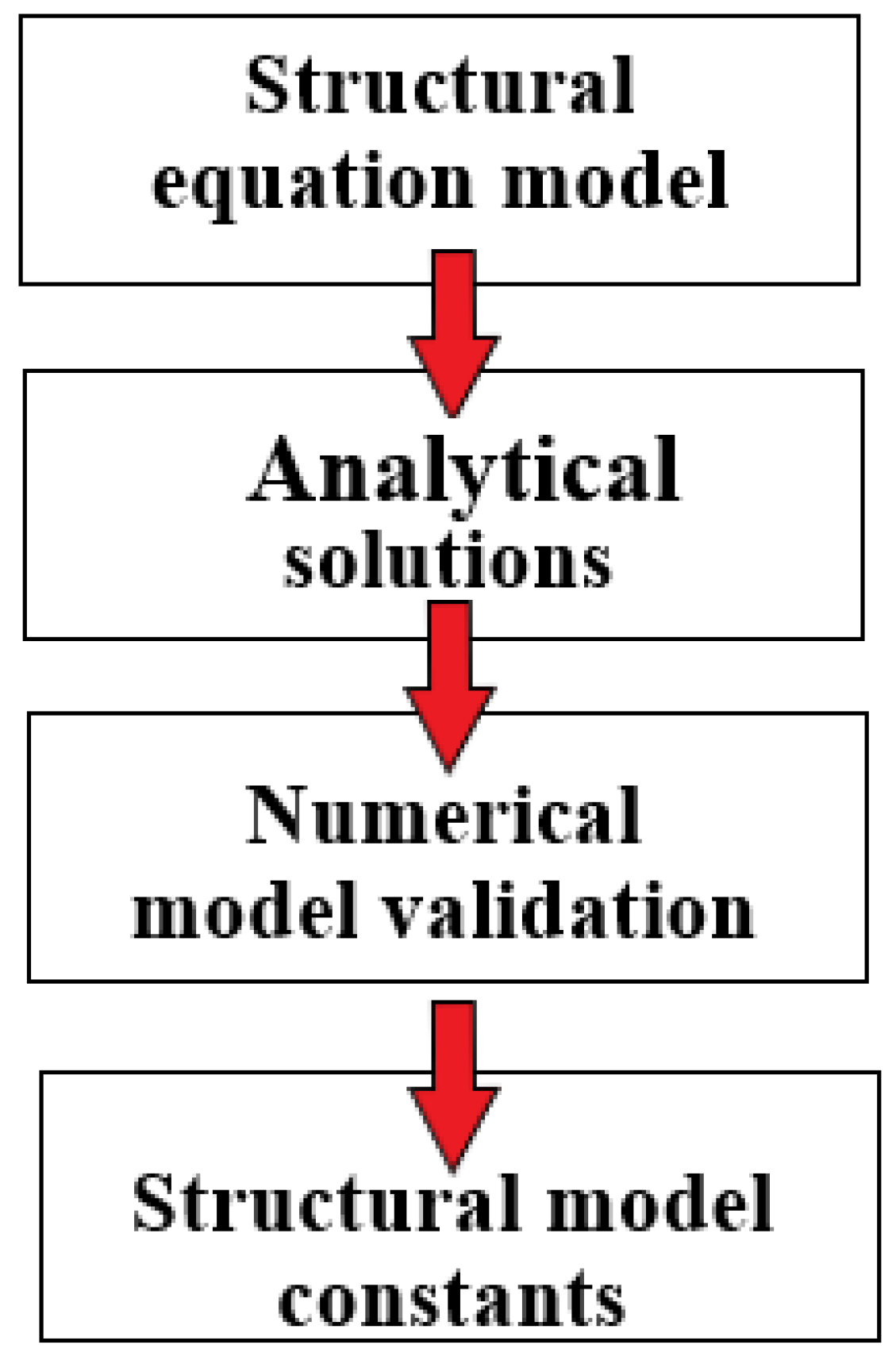
In this context, the present study proposes the development of a nonlinear mathematical model based on paired data describing bacterial dynamics, fungal evolution, and petroleum hydrocarbon degradation, with the aim of rigorously characterizing the bioremediation process and identifying the optimal soil–sludge mixture for maximizing treatment efficiency [11,12,13,14]. The model is solved using a classical Runge–Kutta numerical approach, suitable for time-dependent nonlinear systems [14,15,16,17], and the methodological structure and analysis steps are presented in Figure 1.

Figure 1. Steps of building the mathematical model.

2. Materials and Methods

2.1. Source of Experimental Data and Study Context

The data used in the present study originate entirely from a previously published bioremediation experiment conducted in a heavily petroleum-contaminated area located in Constanța County, Romania. The original experiment included the configuration of biopiles, application of treatments, periodic aeration, and detailed physico-chemical and microbiological analyses. The complete methodology—covering sample collection, preparation of soil–sludge mixtures, analytical procedures, and the instrumentation employed—is described comprehensively in the previously published work [1]. In this study, only the information relevant to the development of the mathematical model is presented, in alignment with current principles of research transparency and reproducibility.

The earlier study demonstrated that the use of dewatered sewage sludge from municipal wastewater treatment plants can significantly enhance the bioremediation of petroleum-contaminated soils by supplying active microorganisms and nutrients. These findings provided the experimental foundation [1,18] for formulating the mathematical proposed model in this work.

2.2. Biopile Configuration and Applied Treatments

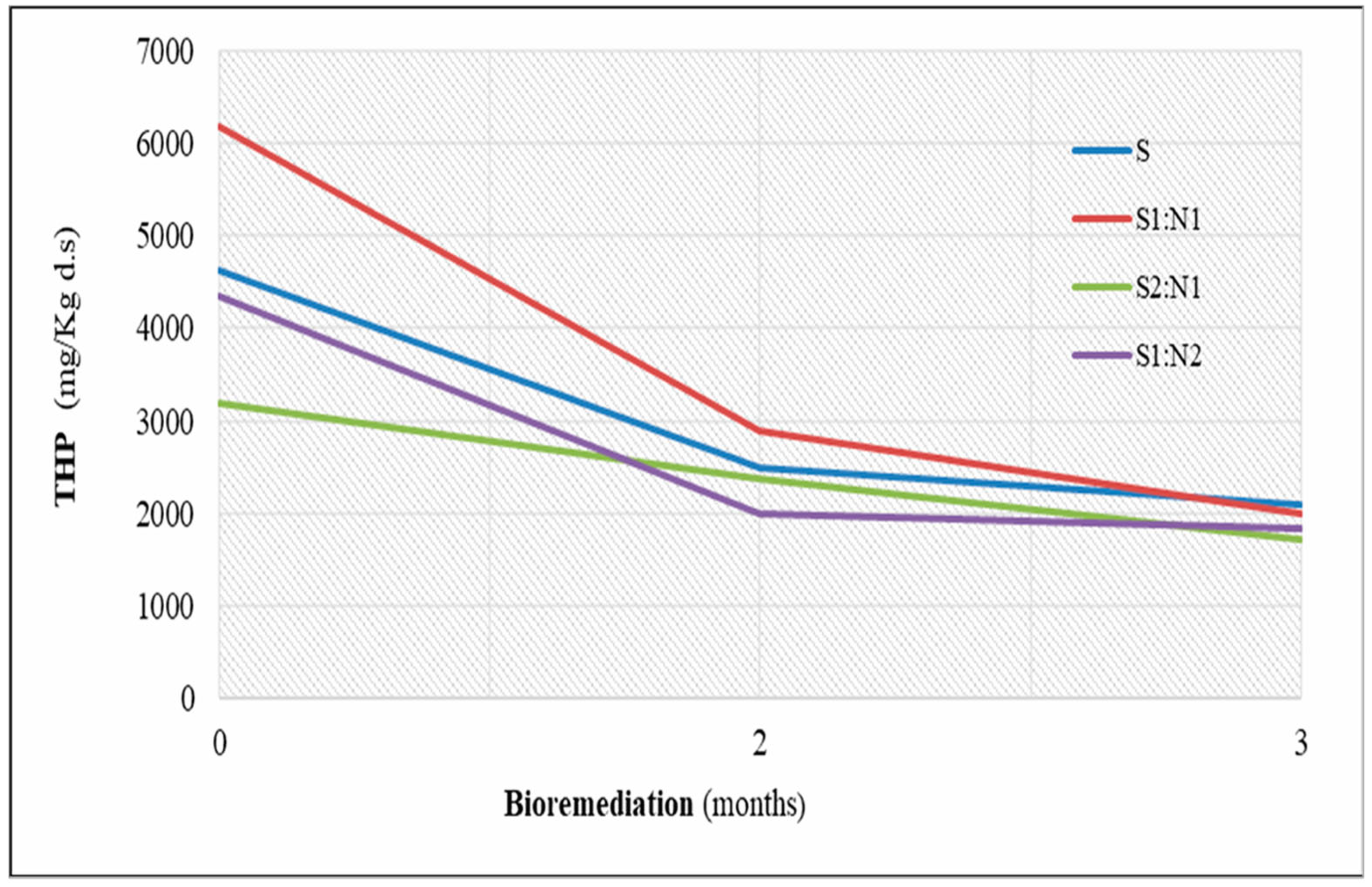
Petroleum-contaminated soil (S) was mixed with dewatered sewage sludge (N) in three distinct volumetric ratios: 1:1 (S1:N1), 2:1 (S2:N1), and 1:2 (S1:N2) (Figure 2). Each mixture was placed in a separate biopile, while untreated contaminated soil served as the control [1].

The biopiles were aerated weekly to ensure adequate oxygenation for microbial activity, following standard practices in assisted bioremediation. Aeration was performed by mechanically turning the material to maintain aerobic conditions favorable for hydrocarbon degradation [1].

2.3. Experimental Variables Used in Mathematical Modeling

2.3.1. Total Petroleum Hydrocarbon (THP) Concentration

THP concentration was determined by infrared (IR) spectroscopy using the InfraCal2 method, following extraction of non-polar compounds with S-316 solvent and removal of polar fractions using activated aluminum oxide. This method is widely applied in bioremediation monitoring due to its sensitivity and reproducibility.

2.3.2. Density of Hydrocarbon-Degrading and Hydrocarbon-Tolerant Bacteria

Enumeration of hydrocarbon-degrading and hydrocarbon-tolerant bacteria was performed using the most probable number (MPN) method, employing minimal medium supplemented with 5% diesel for hydrocarbon-degrading bacteria and LB medium supplemented with 5% diesel for hydrocarbon-tolerant bacteria. Colony viability was confirmed by staining with 0.3% TTC, a standard procedure for assessing microbial metabolic activity.

The soil–sludge mixtures prepared in the defined proportions provided the experimental basis for developing a mathematical model capable of describing the evolution of microbial populations and the degradation of hydrocarbons.

Mathematical modeling is essential for process optimization, as it enables a quantitative description of the fundamental mechanisms governing microbial activity and hydrocarbon degradation, offering insight into the nonlinear dynamics involved.

Figure 2. Evolution of total hydrocarbon concentration (THP) in the four experimental scenarios: S, S1:N1, S2:N1 and S1:N2 [1].

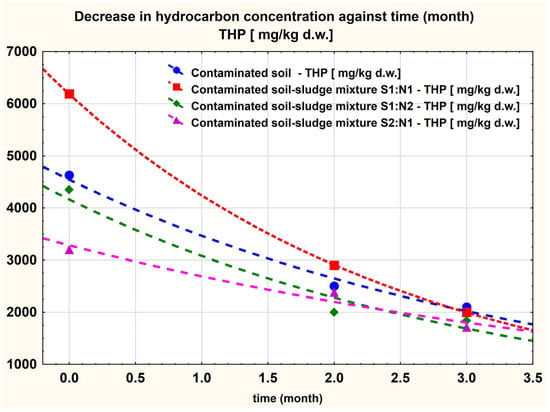
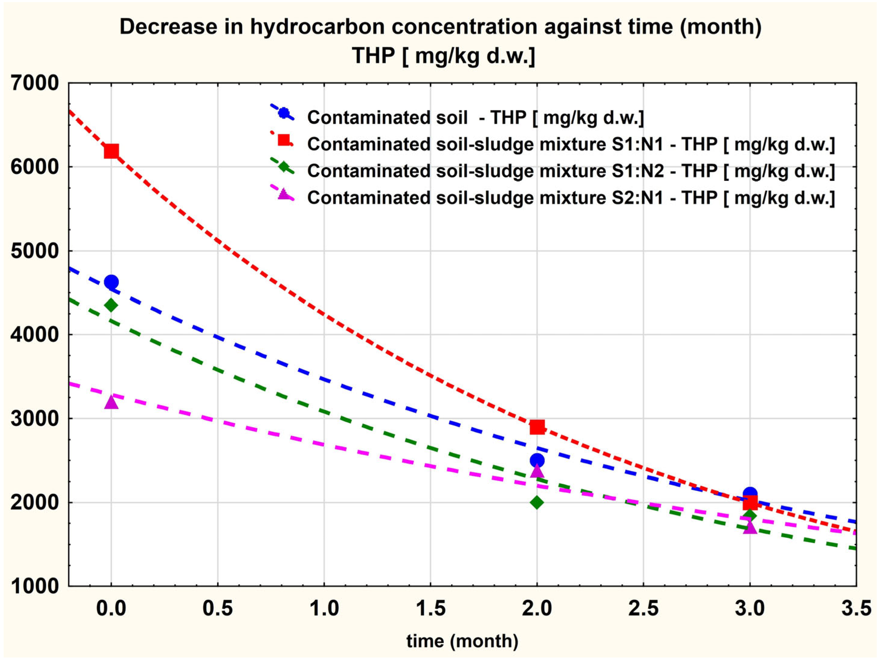
Figure 2. Evolution of total hydrocarbon concentration (THP) in the four experimental scenarios: S, S1:N1, S2:N1 and S1:N2 [1].

2.4. Numerical Methods Approach Used in Bioremediation Modeling

Modeling bioremediation processes requires describing the interactions between hydrocarbon-degrading microorganisms and the available substrate. In this study, the system dynamics are represented by a set of nonlinear differential equations that describe the evolution of hydrocarbon-degrading bacteria, fungi, and substrate concentration. The structure of the model is inspired by Monod-type kinetics [4] and by Lotka–Volterra biological interaction models [13,14], both widely used in microbial ecology.

In this study, the system is represented by three interacting components: hydrocarbon-oxidizing bacteria [13,14,18,19], fungi, and the substrate (total petroleum hydrocarbons). The dynamics of these variables are described using formulations inspired by Monod-type kinetics and Lotka–Volterra biological interaction models, which are frequently applied in microbial ecology to represent competition and cooperation among populations [19,20].

Based on these principles, the evolution equation for the concentration of hydrocarbon-oxidizing bacteria is expressed as follows [20,21,22]:

$${\displaystyle \frac{d}{dt}}B\left(t\right)={\mathit{\mu }}_B{\displaystyle \frac{B\left(t\right)S\left(t\right)}{K_{SB}+S\left(t\right)}}-{\delta }_{B}B\left(t\right)-\alpha B\left(t\right)F\left(t\right),$$

(1)

where

$B=B\left(t\right)$—represents the bacterial concentration, expressed in colony-forming units (CFU) per unit mass.

${\mathit{\mu }}_B$—bacterial growth rate

$K_{SB}$—saturation constant for bacteria

${\delta }_B$—bacterial mortality rate

$\alpha$—inhibition coefficient (arising from the B–F interaction)

$F=F\left(t\right)$—represents the fungal concentration expressed in colony-forming units (CFU) per unit mass.

$S=S\left(t\right)$—represents the substrate concentration.

Equation (1) is a Lotka–Volterra-type expression describing biological populations subjected to elementary interaction processes.

For the evolution of fungal concentration, we considered an equation that reflects evident proportionalities, which can be expressed as:

$${\displaystyle \frac{d}{dt}}F\left(t\right)={\mathit{\mu }}_F{\displaystyle \frac{F\left(t\right)S\left(t\right)}{K_{SF}+S\left(t\right)}}-{\delta }_{F}F\left(t\right)-\beta B\left(t\right)F\left(t\right),$$

(2)

where:

${\mathit{\mu }}_F$—fungal growth rate

$K\_SF$—saturation constant for fungi

${\delta }_F$—fungal mortality rate

$\beta$—inhibition coefficient (arising from the B–F interaction)

Finally, by considering the substrate consumption rates associated with the two types of microorganisms, the evolution rate of this component can be expressed as:

$${\displaystyle \frac{d}{dt}}S\left(t\right)={-q}_B{\displaystyle \frac{B\left(t\right)S\left(t\right)}{K_{SB}+S\left(t\right)}}-q_F{\displaystyle \frac{F\left(t\right)S\left(t\right)}{K_{SF}+S\left(t\right)}},$$

(3)

where:

$q_B$—substrate consumption rate by bacteria

$q_F$—substrate consumption rate by fungi

These equations follow formulations established in the literature, including Lotka–Volterra evolutionary structures, stoichiometric model-based analysis, metabolic network approaches, and generalized distributions [23,24,25].

In the final section, for completeness and comparison, we present the numerical results obtained using a Runge–Kutta algorithm. Thus, considering a partition of the time interval:

$$t_i=\left[t_0, t_1,\dots ,{ t}_k, {.., t}_f\right],$$

For quantities that exhibit temporal evolutions described by expressions of the form:

$${\displaystyle \frac{dy}{dt}}=f(t, y),$$

where $y=y\left(t\right)$ represents the unknown function, with the initial condition $y_0=y\left(t_0\right)$, we can compute, by recurrence, the terms of the series:

$$y_{n+1}=y_n+{\displaystyle \frac{h}{6}}\left(k_1+2·k_2+2·k_3+k_4\right)\mathrm{and} t_{n+1}=t_n+h$$

where

$$\begin{gathered} k_1=f\left(t_n,y_n\right); k_2=f\left(t_n+{\displaystyle \frac{h}{2}},y_n+k_1{\displaystyle \frac{h}{2}}\right); \\ {k}_3=f\left(t_n+{\displaystyle \frac{h}{2}},y_n+k_2{\displaystyle \frac{h}{2}}\right); k_4=f\left(t_n+h,y_n+k_3\right). \end{gathered}$$

A numerical solution of the differential equation can be obtained.

3. Results

3.1. Qualitative Analysis of the System of Equations

The system of differential Equations (1)–(3) describes the interaction between hydrocarbon-oxidizing bacteria, fungi present in the soil–sludge mixture, and the substrate represented by the available hydrocarbons. This system is nonlinear, coupling Monod-type microbial growth processes with Lotka–Volterra interaction terms and with the kinetics of substrate consumption. Due to these nonlinearities, the system does not admit closed-form analytical solutions, a situation frequently encountered in ecological and microbiological models.

Nevertheless, a qualitative analysis allows the identification of several important properties of the system. In the absence of interactions and substrate, Equations (1) and (2) reduce to simple exponential forms, governed by the ratio between the growth rate and the mortality rate. The introduction of Monod saturation terms yields dynamics dependent on substrate availability, while the interaction coefficients α and β introduce reciprocal inhibition mechanisms, reflecting competition for resources and potential antagonistic effects between the two microbial populations.

The system exhibits several equilibrium points, the most relevant being:

(1) The trivial equilibrium $\left(B=0,F=0,S=S_0\right)$, corresponding to a system without microbial activity;

(2) Partial equilibria, in which one population is absent while the other evolves depending on the substrate;

(3) The coexistence equilibrium, in which bacteria, fungi, and substrate reach finite values determined by the model parameters.

The stability of these equilibria depends on the values of the parameters ${\mathit{\mu }}_B, { \mathit{\mu }}_F,{ \delta }_B,{ \delta }_F,{ q}_B,{ q}_F$ and on the initial substrate concentration. In general, for positive parameter values and nonzero initial concentrations, the system exhibits positive and bounded solutions, which is consistent with the biological behavior observed in experiments. Because of the complexity of the nonlinear terms and the coupling between equations, the temporal evolution of the microbial populations and the substrate cannot be expressed analytically. Therefore, numerical integration becomes necessary to obtain approximate solutions and to compare the model with experimental data. The following section presents the numerical simulations performed using the fourth-order Runge–Kutta method, as well as their comparison with the measured experimental evolutions.

3.2. Analytical Approach

To solve the system of Equations (1)–(3), we considered two intermediate steps, applying the method of variation in constants to the homogeneous partial Equations (4) and (5), of the form:

$${\displaystyle \frac{d}{dt}}B\left(t\right)=-{\delta }_{B}B\left(t\right),$$

(4)

and respectively

$${\displaystyle \frac{d}{dt}}F\left(t\right)=-{\delta }_{F}F\left(t\right),$$

(5)

Having elementary solutions of the form (6) for the homogeneous Equation (4),

$$B\left(t\right)=A{·e}^{-{\delta }_{B}t},$$

(6)

and, respectively, solutions of the form (7) for the homogeneous Equation (5),

$$F\left(t\right)=C{·e}^{-{\delta }_{F}t},$$

(7)

In the next step, a well known as the elementary method of variation in constants (the Lagrange method), and thus, a general expression was considered of the form:

$$B\left(t\right)=A(t){·e}^{-{\delta }_{B}t},$$

(8)

and, respectively

$$F\left(t\right)=C\left(t\right){·e}^{-{\delta }_{F}t},$$

(9)

For the general Equation (1), which implies that the growth-rate term for the bacterial concentrations can be computed in the form [24,25,26,27,28]:

$${\displaystyle \frac{d}{dt}}A\left(t\right)=-\alpha A\left(t\right)C\left(t\right){·e}^{-{\delta }_{F}t},$$

(10)

Similarly, for the general case of the evolution of fungal concentrations, we considered a general expression of the form:

$${\displaystyle \frac{d}{dt}}C\left(t\right)=-\beta A\left(t\right)C\left(t\right){·e}^{-{\delta }_{B}t},$$

(11)

In this regard, using the general Equation (1), which describes the evolution of the bacterial population, and applying expressions (11) and (12) while eliminating the identical terms from both sides of Equation (1) and initially neglecting the contribution of the substrate S = S(t), we obtain for fungi, under the conditions of expression (10), the following:

$${\displaystyle \frac{d}{dt}}A\left(t\right)/{\displaystyle \frac{d}{dt}}C\left(t\right)={\displaystyle \frac{\alpha }{\beta }}{·e}^{-{\delta }_{F}t}{·e}^{{\delta }_{B}t},$$

(12)

By defining the discrimination parameter

$$Q={\displaystyle \frac{\alpha }{\beta }}{·e}^{-{\delta }_{F}t}{·e}^{{\delta }_{B}t},$$

(13)

From Equation (3), we obtain the expression for the substrate S = (t) of the form

$$S\left(t\right)={\displaystyle \frac{\frac{d}{dt}A\left(t\right)·K_{SB}}{-\frac{d}{dt}A\left(t\right)+{\mathit{\mu }}_B·A\left(t\right)}}={\displaystyle \frac{\frac{d}{dt}C\left(t\right)·K_{SF}}{-\frac{d}{dt}C\left(t\right)+{\mathit{\mu }}_F·C\left(t\right)}},$$

(14)

Similarly, by considering expressions (10) and (11), we obtain the general equation

$${\displaystyle \frac{\alpha }{\beta }}{\displaystyle \frac{{\alpha ·e}^{-{\delta }_{F}t}{·e}^{{\delta }_{B}t}·\frac{d}{dt}C\left(t\right)·K_{SB}}{\left(-{\frac{\alpha }{\beta }·e}^{-{\delta }_{F}t}{·e}^{{\delta }_{B}t}·\frac{d}{dt}C\left(t\right)·+{\mathit{\mu }}_B·QC\left(t\right)\right)}}={\displaystyle \frac{\frac{d}{dt}C\left(t\right)·K_{SF}}{-\frac{d}{dt}C\left(t\right)+{\mathit{\mu }}_F·C\left(t\right)}},$$

(15)

obtaining the general solutions of the form:

$$C\left(t\right)=a·t^2-b·t,$$

(16)

and, respectively, an approximate solution of the form

$$A\left(t\right)={{\displaystyle \frac{\alpha }{\beta }}·e}^{-{\delta }_{F}t}{·e}^{{\delta }_{B}t}{\displaystyle \frac{\left({\delta }_{B·}t-{\delta }_{F·}t-1\right)}{{\left({\delta }_{B·}t-{\delta }_{F·}t\right)}^2}}+\xi \approx E{e}^{-ct}$$

(17)

And thus, it could be considered the solution of the form:

$$B\left(t\right)E\approx E·\left(a·t^2-b·t\right){·e}^{-c·t},$$

(18)

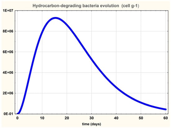
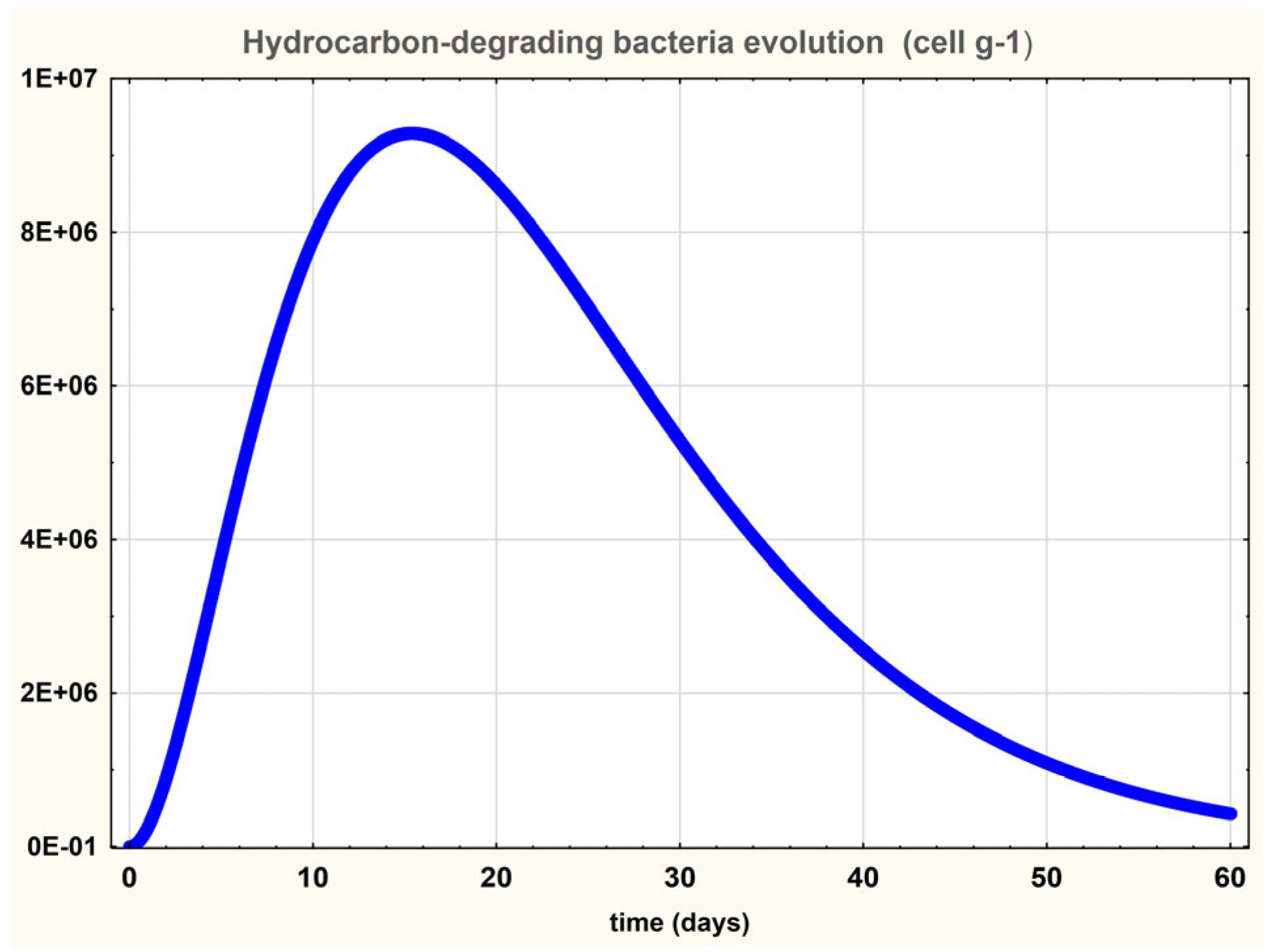
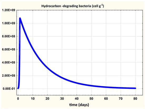
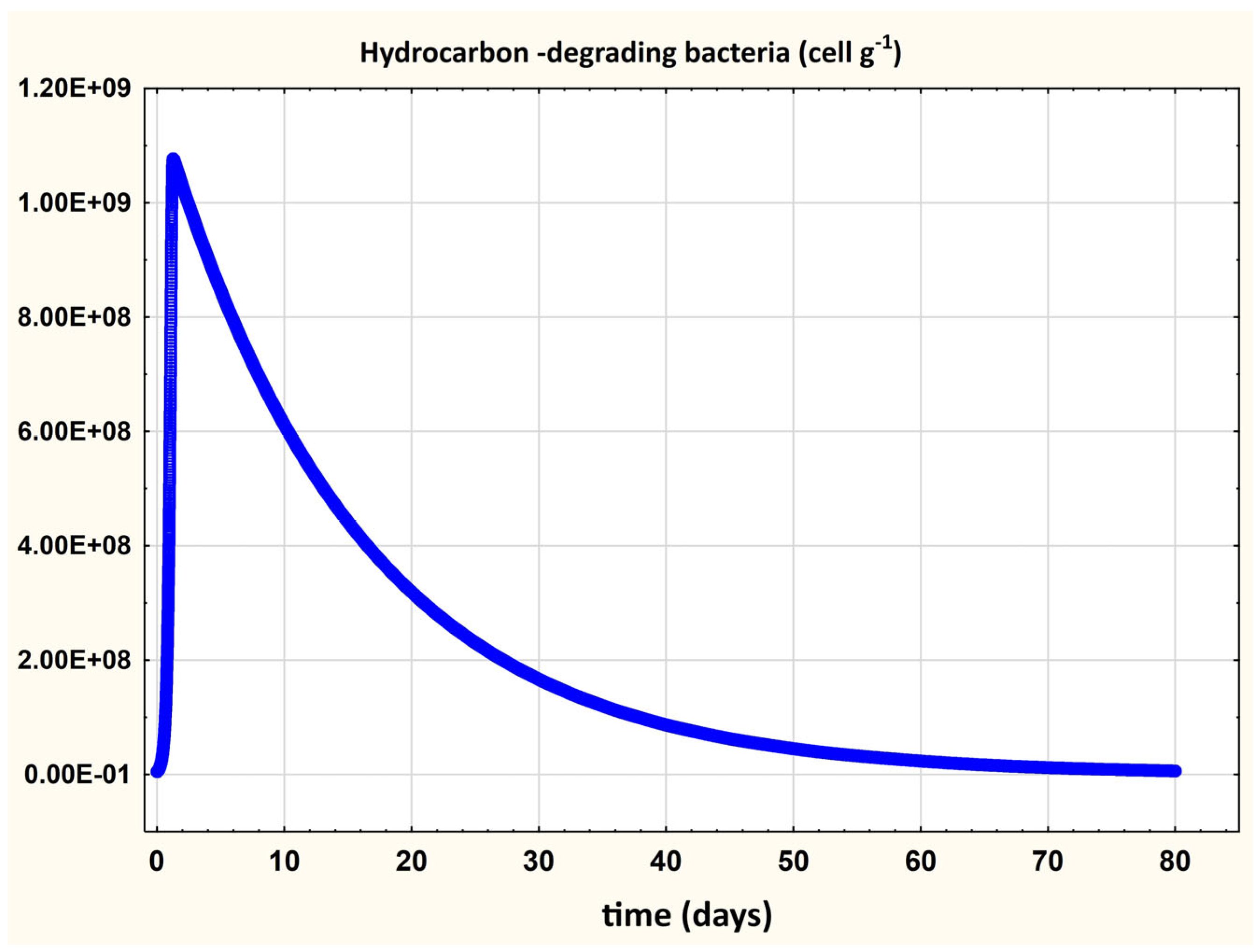
with the generic graphical representation of the form shown in Figure 3.

Figure 3. Temporal evolution of hydrocarbon-degrading bacteria concentration (cells g⁻¹).

These analytical expressions provide qualitative insight into the system’s behavior, but numerical integration remains necessary for accurate comparison with experimental data.

3.3. Results of the Analytical Approach for the Evolution of the Total Amount of Petroleum-Derived Organic Compounds

In Figure 4, the comparative results between the evaluations of the theoretical model and the measurements obtained in the experiment, for the time evolution of the concentrations of hydrocarbon-degrading bacteria, are shown.

Figure 4. Temporal evolution of THP concentration during the experiment.

The theoretical model parameters for each of the four cases considered exhibit a high degree of goodness-of-fit (Table 1), consistent with previous modeling approaches.

Table 1. Goodness-of-fit parameters for THP concentration—Figure 4.

Variant	THP Model	D (mg kg−1 d.w.)	k (month−1)	R2
Contaminated soil	THP = D·exp(−k·x)	4542.35	0.2699	0.9913
Soil–sludge mix S1:N1		6183.33	0.3770	0.9950
Soil–sludge mix S1:N2		4164.46	0.3013	0.9699
Soil–sludge mix S2:N1		3284.56	0.2002	0.9596

The results obtained thus highlighted a clear and sufficiently accurate description of the dynamics of THP within this model.

In the following, we analyze the quality of the model obtained for describing the evolution of hydrocarbon-degrading populations under the conditions defined in the previously conducted experiment.

Using the data from the previously published experiment and applying the analytical expressions (17), it was able to identify the parameters of the analytical model presented in relations (16) and (17), employing a MAPLE script together with the experimentally measured parameters.

Naturally, the theoretical model provides an additional degree of freedom, and for the same set of experimental data, two sets of numerical parameters were found that yield an optimal fit for each individual sample. This additional degree of freedom, which allowed the determination of two compatible solution sets in each of the four experiments performed, led us to the idea of verifying these models of the form (17).

In our case, as is known from the literature, a system of differential equations with the same initial conditions should not have two different solutions if the classical uniqueness conditions (Lipschitz, continuity, etc.) are met. In our case, the system is nonlinear and admits bifurcations. As is known from the literature, in nonlinear systems, such as, e.g., Lotka–Volterra equations, chemical systems, reaction–diffusion models, the following may occur:—bifurcations, multiple stable/unstable solutions, trajectories that separate [29,30,31]. The initial system being of this type, we have a situation in which bifurcated solutions appear.

In what follows, using the experimental data for each experiment in turn, we present the solutions identified for each branch in turn; thus, we can highlight each of the two analytical solutions identified, using the experimental data presented in the cited article and the expression in Equation (17).

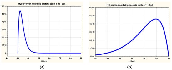
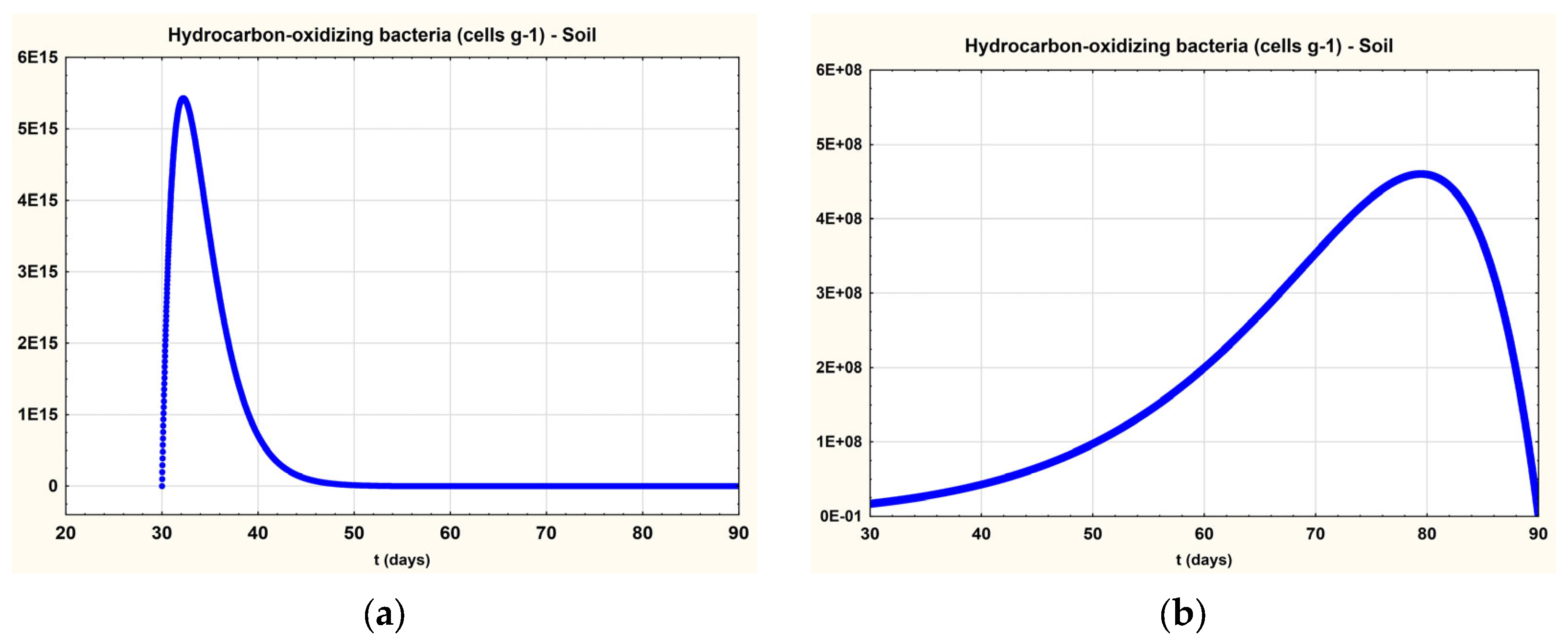
Thus, Figure 5a,b present the results obtained for the soil sample in the case of the two sets of parameters identified based on Equations (14) and (15) and on the experimental values for the first experiment [1].

Figure 5. Temporal evolution of hydrocarbon-degrading bacteria in the soil sample: (a) first set of identified parameters; (b) second set of identified parameters.

Both solutions (Figure 5a,b) are compatible with the imposed initial conditions.

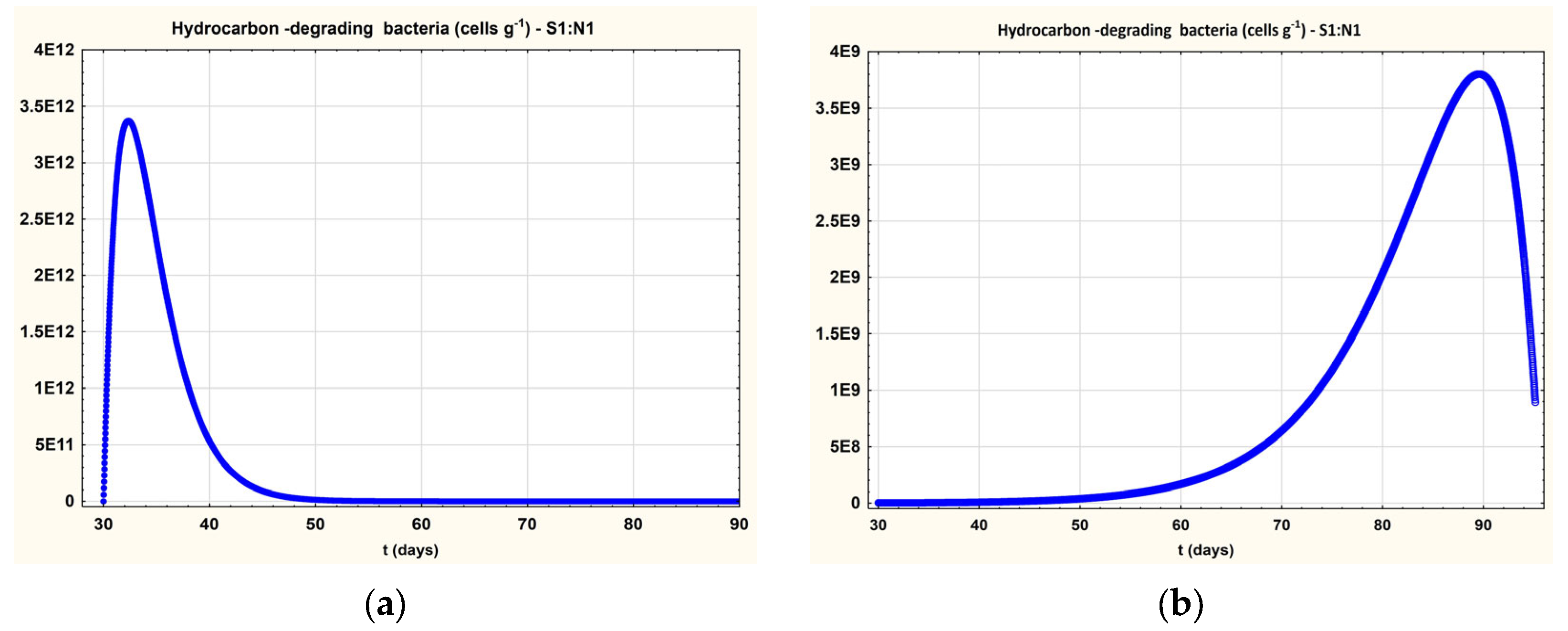
In the following, for the experimental data corresponding to the soil–sludge mixture (v/v) S1:N1 experiment [1], the model results are shown in Figure 6a,b.

Figure 6. Temporal evolution of hydrocarbon-degrading bacteria in the S1:N1 sample: (a) first set of identified parameters; (b) second set of identified parameters.

The existence of multiple compatible solutions is a consequence of the differential equation system and is also evident in the S1:N1 experiment (Lotka–Volterra equations’ bifurcations).

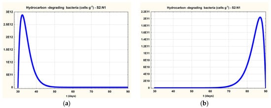
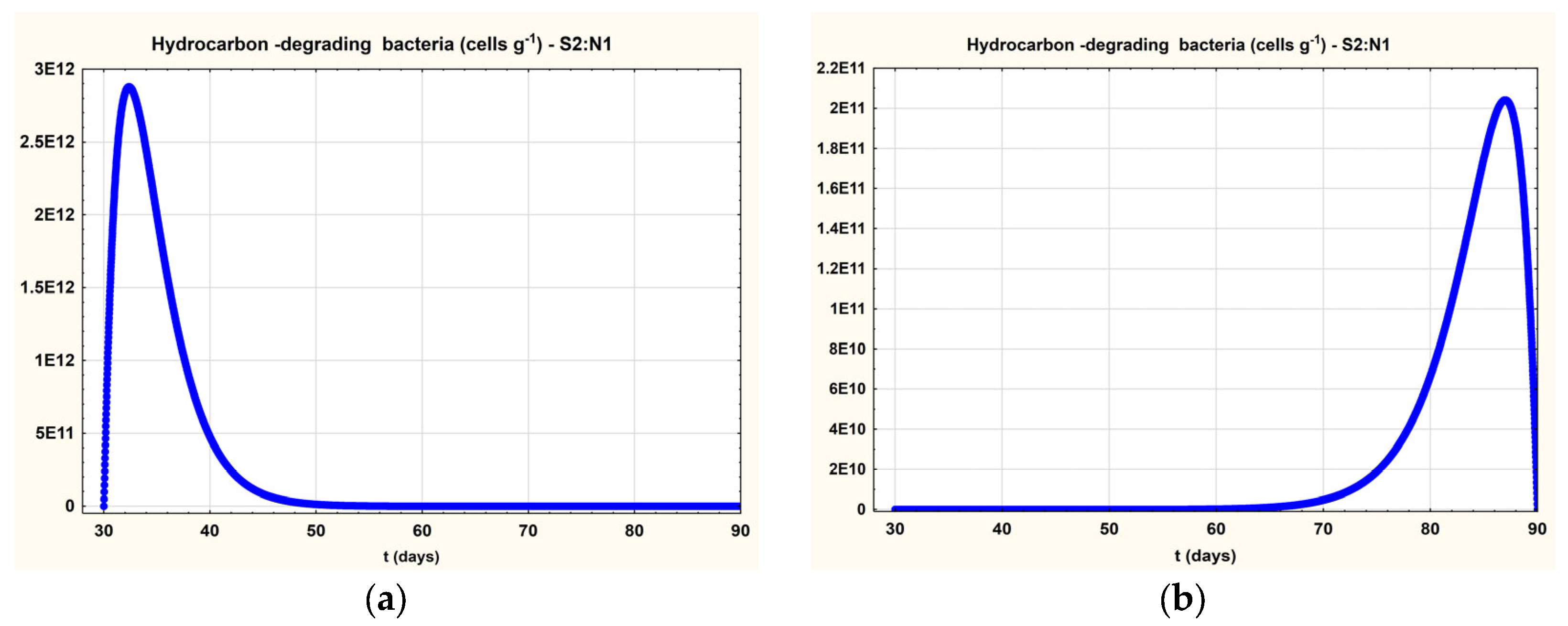
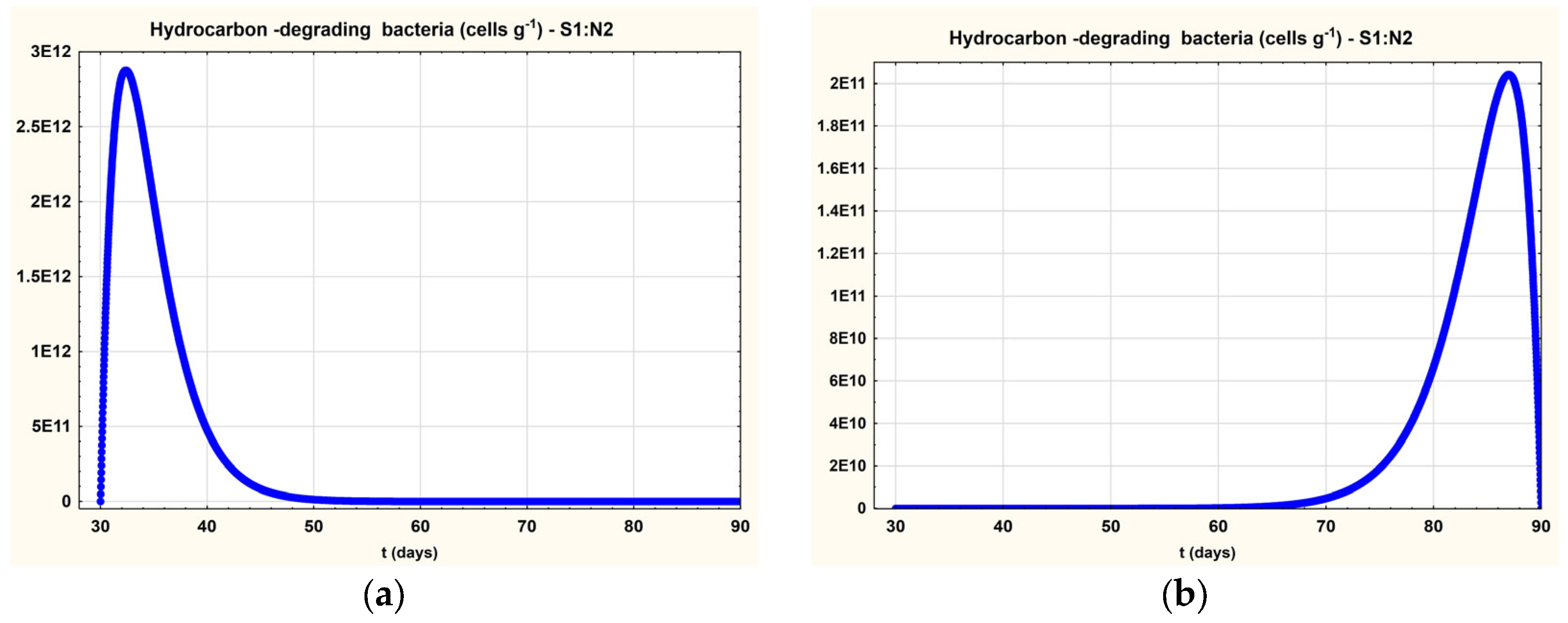
The same state is encountered in the case of the experimental conditions and determinations obtained in the S2:N1 experiment [1] (Figure 7a,b), and for the S1:N2 experiment (Figure 8a,b). By using the experimental data and the considered Equation (17), for the set of experimental measurements corresponding to the soil–sludge mixture (v/v) S1:N2 experiment [1], the results obtained using the described theoretical model are presented in Figure 8a,b.

Figure 7. Temporal evolution of hydrocarbon-degrading bacteria in the S2:N1 sample: (a) first set of identified parameters; (b) second set of identified parameters.

Figure 8. Temporal evolution of hydrocarbon-degrading bacteria in the S1:N2 sample: (a) first set of identified parameters; (b) second set of identified parameters.

Considering the evolution of the moisture content and the results reported in the literature, we retained the accepted coefficient values, which are presented in Table 2. The objective function is the one described in Equation (18) and the evaluation method was, of course, the least squares method.

Table 2. Values of the coefficients identified for the theoretical model (18).

Study Case	Coefficient 1
	a	b	c
Soil	0.4444443689 × 1018	0.1333332993 × 1020	0.4836219232
Soil–sludge mix S1:N1	0.1220703090 × 1018	0.3662109216 × 1019	0.4583657343
Soil–sludge mix S2:N1	0.8656509692 × 1017	0.2596952907 × 1019	0.4526373927
Soil–sludge mixt S1:N2	0.646307626 × 1017	0.2134913923 × 1019	0.4315372312

¹ The determined coefficients for analytical solution (18).

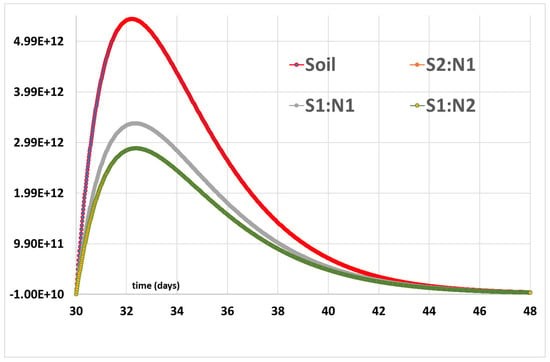
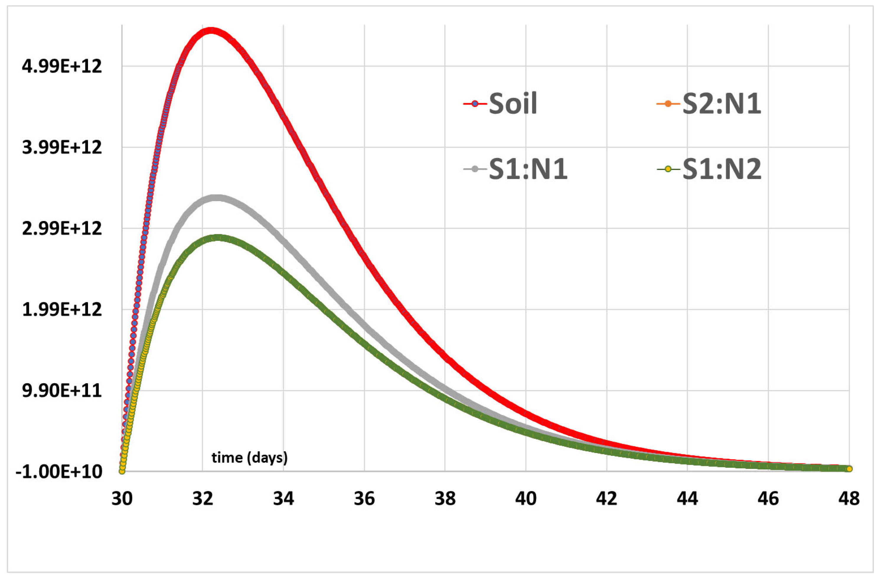
The R² values for these models are higher than R² = 0.998. Figure 9 presents, for comparison, all four models obtained. A clear evolution of the characteristics can be observed for each individual case.

Figure 9. Temporal evolution of hydrocarbon-degrading bacteria concentration for the four experimental cases.

Thus, for the concentration of hydrocarbon-degrading bacteria (cells g⁻¹), using the theoretical model, the concentration dynamics can be represented for the four cases studied: the soil sample, the soil–sludge mixture (v/v) S1:N1, the soil–sludge mixture (v/v) S2:N1, and the soil–sludge mixture (v/v) S1:N2.

3.4. Numerical Approach Method

Considering a numerical approach and using a fourth-order classical Runge–Kutta algorithm [32,33,34,35], a numerical procedure for solving the coupled differential Equations (1)–(3) could be implemented. In this context, for Equation (1), we can write the following expression:

$${\displaystyle \frac{d}{dt}}B\left(t\right)={\mathit{\mu }}_B{\displaystyle \frac{B\left(t\right)S\left(t\right)}{K_{SB}+S\left(t\right)}}-{\delta }_{B}B\left(t\right)-\alpha B\left(t\right)F\left(t\right)\equiv f_{B }\left(t, B,S,F\right),$$

(19)

Similarly for fungi:

$${\displaystyle \frac{d}{dt}}F\left(t\right)={\mathit{\mu }}_F{\displaystyle \frac{F\left(t\right)S\left(t\right)}{K_{SF}+S\left(t\right)}}-{\delta }_{F}F\left(t\right)-\beta B\left(t\right)F\left(t\right)\equiv f_{F }\left(t, F,S,B\right),$$

(20)

And for substrate:

$${\displaystyle \frac{d}{dt}}S\left(t\right)={-q}_B{\displaystyle \frac{B\left(t\right)S\left(t\right)}{K_{SB}+S\left(t\right)}}-q_F{\displaystyle \frac{F\left(t\right)S\left(t\right)}{K_{SF}+S\left(t\right)}}\equiv f_{S }\left(t, S,F,B\right),$$

(21)

where $B=B\left(t\right), F=F\left(t\right) \mathrm{a}\mathrm{n}\mathrm{d} S=S\left(t\right),$represent the unknown functions, with initial conditions of the form $B_0=B\left(t_0\right)$, $F_0=F\left(t_0\right)$ and $S_0=S\left(t_0\right)$ respectively.

The implementation of the fourth-order Runge–Kutta algorithm allows the recursive computation of the solution, the terms of the series being given by the following expressions:

$$t_{n+1}=t_n+h,$$

(22)

$$B_{n+1}=B_n+{\displaystyle \frac{h}{6}}·\left(k_{B1}+2·k_{B2}+2·k_{B3}+k_{B4}\right),$$

(23)

$$F_{n+1}=F_n+{\displaystyle \frac{h}{6}}·\left(k_{F1}+2·k_{F2}+2·k_{F3}+k_{F4}\right),$$

(24)

and respectively

$$S_{n+1}={FS}_n+{\displaystyle \frac{h}{6}}·\left(k_{S1}+2·k_{S2}+2·k_{S3}+k_{S4}\right),$$

(25)

where

$$k_{B1}=f_{B }\left(t_n, B_n,S_n,F_n\right); k_{F1}=f_{F }\left(t_n, F_n,S_n,B_n\right); k_{S1}=f_{S }\left(t_n, S_n,F_n,B_n\right),$$

(26)

and respectively

$$\begin{gathered} k_{B2}=f_{B }\left(t_n+{\displaystyle \frac{h}{2}}, B_n{+k}_{B1}{\displaystyle \frac{h}{2}},S_{n } {+k}_{S1}{\displaystyle \frac{h}{2}},F_n+k_{F1}{\displaystyle \frac{h}{2}}\right); \\ {k}_{F2}=f_{F }\left(t_n+{\displaystyle \frac{h}{2}}, F_n{+k}_{F1}{\displaystyle \frac{h}{2}},S_{n } {+k}_{S1}{\displaystyle \frac{h}{2}},B_n+k_{B1}{\displaystyle \frac{h}{2}}\right); \\ {k}_{S2}=f_{S }\left(t_n+{\displaystyle \frac{h}{2}}, S_n{+k}_{S1}{\displaystyle \frac{h}{2}},F_{n } {+k}_{F1}{\displaystyle \frac{h}{2}},B_n+k_{B1}{\displaystyle \frac{h}{2}}\right), \end{gathered}$$

(27)

and respectively

$$\begin{gathered} k_{B3}=f_{B }\left(t_n+{\displaystyle \frac{h}{2}}, B_n{+k}_{B2}{\displaystyle \frac{h}{2}},S_{n } {+k}_{S2}{\displaystyle \frac{h}{2}},F_n+k_{F2}{\displaystyle \frac{h}{2}}\right); \\ {k}_{F3}=f_{F }\left(t_n+{\displaystyle \frac{h}{2}}, F_n{+k}_{F2}{\displaystyle \frac{h}{2}},S_{n } {+k}_{S2}{\displaystyle \frac{h}{2}},B_n+k_{B2}{\displaystyle \frac{h}{2}}\right); \\ {k}_{S3}=f_{S }\left(t_n+{\displaystyle \frac{h}{2}}, S_n{+k}_{S2}{\displaystyle \frac{h}{2}},F_{n } {+k}_{F2}{\displaystyle \frac{h}{2}},B_n+k_{B2}{\displaystyle \frac{h}{2}}\right), \end{gathered}$$

(28)

and respectively

$$\begin{gathered} k_{B4}=f_{B }\left(t_n+h, B_n{+k}_{B3}h,S_{n } {+k}_{S3}h,F_n+k_{F3}h\right); \\ {k}_{F4}=f_{F }\left(t_n+h, F_n{+k}_{F3}h,S_{n } {+k}_{S3}h,B_n+k_{B3}h\right); \\ {k}_{S4}=f_{S }\left(t_n+h, S_n{+k}_{S3}h,F_{n } {+k}_{F3}h,B_n+k_{B3}h\right). \end{gathered}$$

(29)

In this way, by implementing the algorithm described in the system of relations (19)–(26), the numerical simulations of Equations (1)–(3) can be obtained [36,37,38].

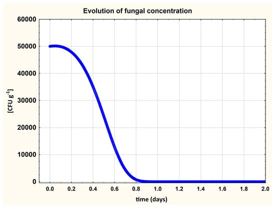
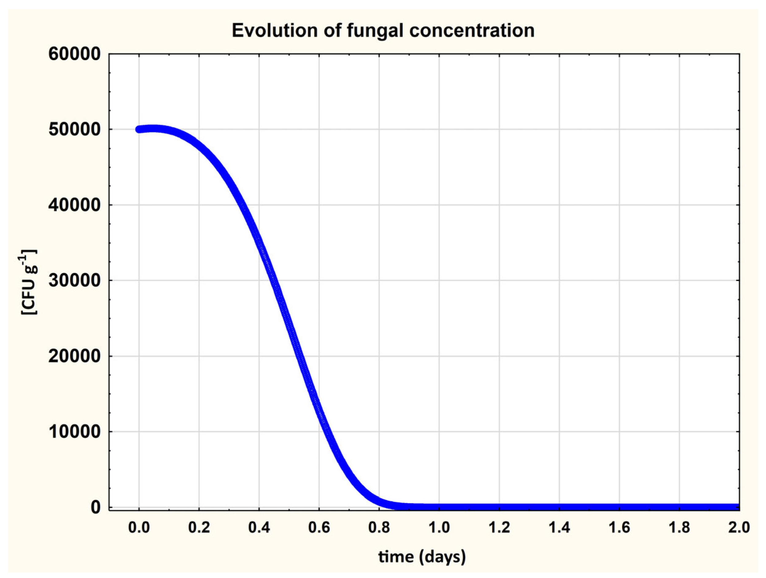
Figure 10 presents the temporal evolution of hydrocarbon-degrading bacteria concentration obtained using the Runge–Kutta integration scheme [38,39]. The related coefficients are presented in Table 3. The numerical simulations were repeated, considering the best value for R-square as the optimization criterion, for a better fit with the experimental data. (Figure 10 for the dynamics of the evolution of the bacterial concentration, respectively, Figure 11 for the dynamics of the fungal concentration).

Figure 10. Representation of the temporal evolution of hydrocarbon-degrading bacteria concentration (cells g⁻¹).

Table 3. Parameter values fitted using the numerical solution of the differential Equations (22)–(28)—Runge–Kutta model parameters.

Case Study	${\mathit{\mu }}_{\mathit{B}}$*	${\mathit{K}}_{\mathit{S}\mathit{B}}$*	${\mathit{\delta }}_{\mathit{B}}$*	${\mathit{\mu }}_{\mathit{F}}\mathit{*}$	${\mathit{K}}_{\mathit{S}\mathit{F}}$*	${\mathit{\delta }}_{\mathit{F}}$*
Soil	5.49	240000	0.065	0.62	30	0.0000001
Soil–sludge mix S1:N1	5.482	245000	0.065	0.62	30	0.0000001
Soil–sludge mix S2:N1	5.464	248000	0.065	0.62	30	0.0000001
Soil–sludge mix S1:N2	5.349	262000	0.065	0.62	30	0.0000001

* The Runge–Kutta 4 simulation’s coefficients.

Figure 11. Representation of the temporal evolution of fungal concentration (CFU g⁻¹).

The most difficult problem was the one related to the integration step, in order to avoid the numerical instability, which is specific to these processes.

For all the cases considered, we made the following attributions, $q_B=0.01$ (substrate consumption rate by bacteria) and $q_F=0.03 ($substrate consumption rate by fungi), while the $\alpha$—inhibition coefficient (arising from the B–F interaction), and $\beta$—inhibition coefficient (arising from the B–F interaction) were considered with equal value as 0.0000001. The time step was considered as $h=∆t=0.002 (over \mathrm{40,000} iterations)$.

Numerous numerical simulations were made, the integration step being adapted (by recursive reduction) to each simulation, because the Runge–Kutta integration, even the fourth-order one, proved to be extremely unstable.

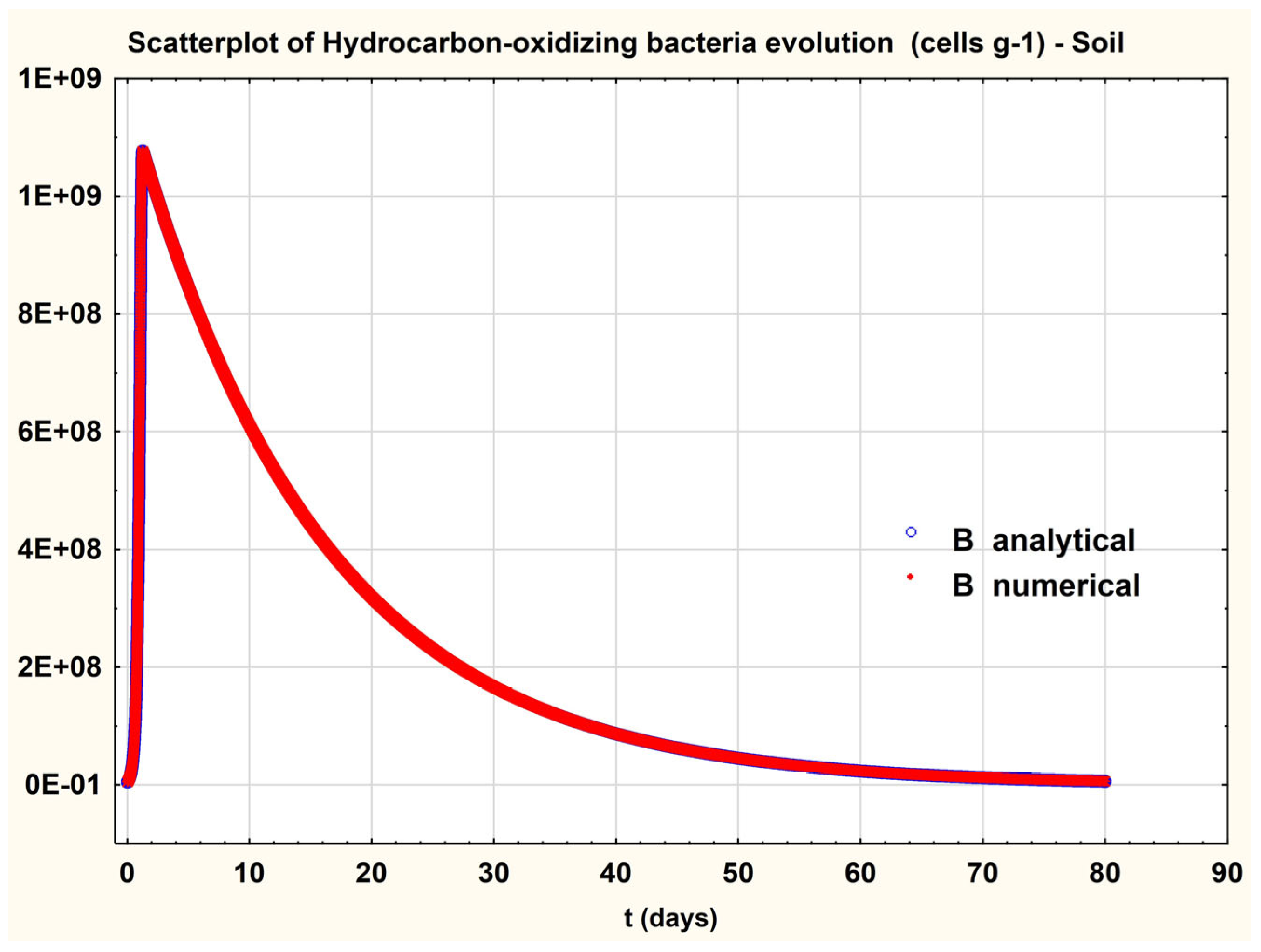
Figure 12 presents the comparison of the numerical and analytical solutions for the first experiment models. Obviously, it is observed that, except for the marginal areas where the two models differ very little, the models can be considered comparable (Figure 12).

Figure 12. Representation of the temporal evolution of hydrocarbon-degrading bacteria concentration (cells g⁻¹) in a comparative approach—analytical and numerical results.

Considering these results, it can be considered comparable [40,41], with sufficient precision. In this case, it could be considered that this strategy could be considered as effective.

4. Discussion

Biodegradation was represented by a Monod-type kinetic term, and the modeling approach was based on a system of coupled differential equations with a Lotka–Volterra-type structure [2]. Based on these equations, analytical solutions were developed and proved to be efficient, and for comparison, a numerical solution using the fourth-order Runge–Kutta method was also proposed. The analytical model generated two sets of compatible solutions for each experimental case, a behavior characteristic of nonlinear systems and associated with the presence of bifurcations, multiple stable or unstable trajectories, and divergent solutions.

This phenomenon is consistent with theoretical expectations for nonlinear differential systems and confirms the complexity of the interactions between hydrocarbon-degrading bacteria, fungi, and substrate. The numerical simulations obtained using the Runge–Kutta method allowed the comparison of model predictions with the experimental data.

The high R-square values (>0.998) indicate that both the analytical and numerical approaches provide an adequate representation of the bioremediation process under the studied conditions [2,3,42,43].

4.1. Advantages

The numerical approach captures nonlinear interactions between microbial populations and substrate dynamics while maintaining a relatively simple computational structure.

The fourth-order Runge–Kutta method provides good accuracy for a given integration step and is straightforward to apply in simulations.

The analytical model offers closed-form expressions that facilitate rapid evaluation of system behavior under different conditions.

The strong agreement between model predictions and experimental data confirms the robustness of both approaches.

The combined modeling framework supports the interpretation of biodegradation processes in complex soil–sludge systems [4].

4.2. Important Limitations

The system of equations is stiff, and explicit numerical schemes such as the classical Runge–Kutta method may become unstable unless very small integration steps are used.

Nonlinear systems of this type may exhibit bifurcations and multiple compatible solutions, complicating parameter identification and model validation.

The analytical model, although efficient, may oversimplify certain environmental interactions that are not explicitly included in the equations.

The numerical simulations require repeated adjustments of the integration step to maintain stability, increasing the computational effort.

The presence of multiple solution branches reflects the inherent complexity of the system and may limit the predictive capacity of the model outside the calibrated domain.

Despite these limitations, the combined use of experimental data, analytical modeling, and numerical simulations provides a comprehensive understanding of the bioremediation process and supports the optimization of treatment strategies for petroleum-contaminated soils. Building on these methodological considerations, it is useful to situate the use of sludge-based remediation materials within a broader framework of resource management and environmental protection, given that the origin and characteristics of the sludge can influence both the efficiency of the process and its ecological implications.

From a broader environmental management perspective, the use of sewage sludge in bioremediation aligns with the principles of the circular economy, where secondary resource flows are reintegrated into productive cycles, consistent with recent analyses of economic, technological, and environmental drivers of circularity within the European Union [39]. At the same time, the literature highlights the need to monitor potential contaminants associated with wastewater effluents, including heavy metals, given their capacity to accumulate in natural water systems [42]. These considerations provide a wider conceptual framework for evaluating the environmental implications of using sludge-derived materials in remediation applications.

5. Conclusions

In this article, we analyzed a nonlinear Lotka–Volterra–type system of differential equations describing the interaction between hydrocarbon-degrading bacteria and substrate, in which biodegradation was represented through a Monod-type kinetic term. The structure of the model allowed the formulation of simple analytical solutions, which proved effective in interpreting the system’s behavior. The main difficulty arose from the nonlinear nature of the equations, which may lead to bifurcations and the existence of multiple compatible solutions.

To obtain a comparative solution, we also implemented a numerical approach for integrating the system of differential equations. Temporal integration was performed using an explicit scheme with a time step adapted to satisfy the stability conditions imposed by the model terms. This stage required the highest computational effort, as numerical stability was sensitive to the choice of integration step. The biodegradation term was evaluated at each time step based on the local substrate concentration, according to Monod kinetics.

The results showed that both analytical and numerical solutions can adequately describe the evolution of the system under the analyzed conditions. In the future, we intend to develop a software tool that will allow the automatic evaluation of bacterial and substrate concentration dynamics, extending the model to include a larger number of coupled differential equations.

Additionally, the modeling framework presented here can be further enhanced by integrating environmental variability, parameter uncertainty, and microbial community interactions. Such extensions would improve the predictive capacity of the model and support its application to real contaminated sites, where biodegradation processes are influenced by complex and dynamic ecological factors.

In future works, we will revisit the problem using Python scripts and MATLAB Version 2020, respectively, for the use of different solvers.

References

- Iorga, C.M.; Georgescu, L.P.; Ungureanu, C.; Stancu, M.M. Sustainable Remediation of Polluted Soils from the Oil Industry Using Sludge from Municipal Wastewater Treatment Plants. Processes 2025, 13, 245. [Google Scholar] [CrossRef] [Scilit]
- Lifshits, S.; Glyaznetsova, Y.; Erofeevskaya, L.; Chalaya, O.; Zueva, I. Effect of Oil Pollution on the Ecological Condition of Soils and Bottom Sediments of the Arctic Region (Yakutia). Environ. Pollut. 2021, 288, 117680. [Google Scholar] [CrossRef] [Scilit]
- Kalia, A.; Sharma, S.; Semor, N.; Babele, P.K.; Sagar, S.; Bhatia, R.K.; Walia, A. Recent advancements in hydrocarbon bioremediation and future challenges. 3 Biotech 2022, 12, 135. [Google Scholar] [CrossRef] [Scilit] [PubMed]
- Monod, J. The Growth of Bacterial Populations. Cold Spring Harb. Symp. Quant. Biol. 1959, 24, 249–260. [Google Scholar]
- Truskewycz, A.; Gundry, T.D.; Khudur, L.S.; Kolobaric, A.; Taha, M.; Aburto-Medina, A.; Ball, A.S.; Shahsavari, E. Petroleum Hydrocarbon Contamination in Terrestrial Ecosystems—Fate and Microbial Responses. Molecules 2019, 24, 3400. [Google Scholar] [CrossRef] [Scilit] [PubMed]
- Gonze, D.; Coyte, K.Z.; Lahti, L.; Faust, K. Microbial Communities as Dynamical Systems. Curr. Opin. Microbiol. 2018, 44, 41–49. [Google Scholar] [CrossRef] [Scilit]
- Ayilara, M.S.; Babalola, O.O. Bioremediation of Environmental Wastes: The Role of Microorganisms. Front. Agron. 2023, 5, 1183691. [Google Scholar] [CrossRef] [Scilit]
- Martins, G.; Campos, S.; Ferreira, A.; Castro, R.; Duarte, M.S.; Cavaleiro, A.J. A Mathematical Model for Bioremediation of Hydrocarbon Contaminated Soils. Appl. Sci. 2022, 12, 11069. [Google Scholar] [CrossRef] [Scilit]
- Stancu, M.M. Investigating the Potential of Native Soil Bacteria for Diesel Biodegradation. Microorganisms 2025, 13, 564. [Google Scholar] [CrossRef] [Scilit]
- Das, N.; Chandran, P. Microbial Degradation of Petroleum Hydrocarbon Contaminants: An Overview. Biotechnol. Res. Int. 2011, 2011, 941810. [Google Scholar] [CrossRef] [Scilit]
- Aslam, K.; Saeed, H.I.; Alyas, J.; Saeed, A.; Majeed, T.; Anjum, I. Role of Microorganisms in Bioremediation. Int. J. Environ. Sci. Technol. 2021, 18, 543–556. [Google Scholar] [CrossRef] [Scilit]
- Abatenh, E.; Gizaw, B.; Tsegaye, Z.; Wassie, M. The Role of Microorganisms in Bioremediation—A Review. Open J. Environ. Biol. 2017, 2, 38–46. [Google Scholar] [CrossRef] [Scilit]
- Huang, L. Optimization of a New Mathematical Model for Bacterial Growth. Food Control 2013, 32, 283–288. [Google Scholar] [CrossRef] [Scilit]
- Chukwuka, K.S.; Alimba, C.G.; Ataguba, G.A.; Jimoh, W.A. The Impacts of Petroleum Production on Terrestrial Fauna and Flora in the Oil-Producing Region of Nigeria. In The Political Ecology of Oil and Gas Activities in the Nigerian Aquatic Ecosystem; Elsevier: Amsterdam, The Netherlands, 2018; pp. 125–142. [Google Scholar]
- Matilda, M.I.; Samuel, H.S. Bioremediation of oil spill: Concept, methods and applications. Discov. Chem. 2024, 1, 42. [Google Scholar] [CrossRef] [Scilit]
- Shah, S.; Yadav, R. Oil Eating Microbes: A Boon for Environmental Cleaning. Environ. Biotechnol. J. 2018, 12, 45–52. [Google Scholar]
- Larsen, P.; Hamada, Y.; Gilbert, J. Modeling microbial communities: Current, developing, and future technologies for predicting microbial community interaction. J. Biotechnol. 2012, 160, 17–24. [Google Scholar] [CrossRef] [Scilit]
- Baranyi, J.; Roberts, T.A. A Dynamic Approach to Predicting Bacterial Growth in Food. Int. J. Food Microbiol. 1994, 23, 277–294. [Google Scholar] [CrossRef] [Scilit]
- Song, H.-S.; Cannon, W.; Beliaev, A.; Konopka, A. Mathematical Modeling of Microbial Community Dynamics: A Methodological Review. Processes 2014, 2, 711–752. [Google Scholar] [CrossRef] [Scilit]
- Varjani, S.J. Microbial degradation of petroleum hydrocarbons. Bioresour. Technol. 2017, 223, 277–286. [Google Scholar] [CrossRef] [Scilit]
- De Jong, H.; Casagranda, S.; Giordano, N.; Cinquemani, E.; Ropers, D.; Geiselmann, J.; Gouzé, J.-L. Mathematical Modelling of Microbes: Metabolism, Gene Expression and Growth. J. R. Soc. Interface 2017, 14, 20170502. [Google Scholar] [CrossRef] [Scilit]
- Song, H.-S. Special Issue: Microbial Community Modeling: Prediction of Microbial Interactions and Community Dynamics. Processes 2018, 6, 41. [Google Scholar] [CrossRef] [Scilit]
- Lenart, A. The Gompertz Distribution and Maximum Likelihood Estimation of Its Parameters—A Revision; Max Planck Institute for Demographic Research: Rostock, Germany, 2012; Available online: https://www.demogr.mpg.de/papers/working/wp-2012-008.pdf (accessed on 16 January 2026).
- Schnoor, J.L.; Licht, L.A.; McCutcheon, S.C.; Wolfe, N.L.; Carreira, L.H. Phytoremediation of organic and nutrient contaminants. Environ. Sci. Technol. 1995, 29, 318A–323A. [Google Scholar] [CrossRef] [PubMed]
- Sayler, G.S.; Ripp, S. Field applications of genetically engineered microorganisms for bioremediation processes. Curr. Opin. Biotechnol. 2000, 11, 286–289. [Google Scholar] [CrossRef] [Scilit] [PubMed]
- Hassanshahian, M.; Emtiazi, G.; Caruso, G.; Cappello, S. Bioremediation (bioaugmentation/biostimulation) trials of oil polluted seawater: A mesocosm simulation study. Mar. Environ. Res. 2014, 95, 28–38. [Google Scholar] [CrossRef] [Scilit] [PubMed]
- Huang, L. Growth kinetics of Listeria monocytogenes in broth and beef frankfurters--determination of lag phase duration and exponential growth rate under isothermal conditions. J. Food Sci. 2008, 73, E235–E242. [Google Scholar] [CrossRef] [Scilit] [PubMed]
- Baldera-Moreno, Y.; Pino, V.; Farres, A.; Banerjee, A.; Gordillo, F.; Andler, R. Biotechnological Aspects and Mathematical Modeling of the Biodegradation of Plastics under Controlled Conditions. Polymers 2022, 14, 375. [Google Scholar] [CrossRef] [Scilit]
- Goh, B.S. Global stability in many-species systems. Am. Nat. 1977, 111, 135–143. [Google Scholar] [CrossRef] [Scilit]
- Hofbauer, J.; Sigmund, K. Evolutionary Games and Population Dynamics; Cambridge University Press: Cambridge, UK, 1998. [Google Scholar]
- Fisher, C.K.; Mehta, P. Identifying keystone species in the human gut microbiome from metagenomic timeseries using sparse linear regression. PLoS Comput. Biol. 2014, 10, e0102451. [Google Scholar] [CrossRef] [Scilit]
- Jin, Q. Building microbial kinetic models for environmental application: A theoretical perspective. Appl. Geochem. 2023, 158, 105782. [Google Scholar] [CrossRef] [Scilit]
- Chandel, A.K.; Jiang, L.; Luo, Y. Microbial Models for Simulating Soil Carbon Dynamics: A Review. J. Geophys. Res. Biogeosci. 2023, 128, e2023JG007436. [Google Scholar] [CrossRef] [Scilit]
- Saeed, M.; Ilyas, N.; Bibi, F.; Shabir, S.; Jayachandran, K.; Sayyed, R.Z.; Shati, A.A.; Alfaifi, M.Y.; Show, P.L.; Rizvi, Z.F. Development of novel kinetic model based on microbiome and biochar for in-situ remediation of total petroleum hydrocarbons (TPHs) contaminated soil. Chemosphere 2023, 324, 138311. [Google Scholar] [CrossRef] [Scilit] [PubMed]
- Zhou, H.; Liu, Q.; Jiang, L.; Shen, Q.; Chen, C.; Zhang, C.; Tang, J. Enhanced remediation of oil-contaminated intertidal sediment by bacterial consortium of petroleum degraders and biosurfactant producers. Chemosphere 2023, 330, 138763. [Google Scholar] [CrossRef] [Scilit] [PubMed]
- Tripathi, V.; Gaur, V.K.; Thakur, R.S.; Patel, D.K.; Manickam, N. Assessing the half-life and degradation kinetics of aliphatic and aromatic hydrocarbons by bacteria isolated from crude oil contaminated soil. Chemosphere 2023, 337, 139264. [Google Scholar] [CrossRef] [Scilit] [PubMed]
- Raajaraam, L.; Raman, K. Modeling Microbial Communities: Perspective and Challenges. ACS Synth. Biol. 2024, 13, 2260–2270. [Google Scholar] [CrossRef] [Scilit]
- Kettle, H.; Holtrop, G.; Louis, P.; Flint, H.J. microPop: Modelling microbial populations and communities in R. Methods Ecol. Evol. 2018, 9, 399–409. [Google Scholar] [CrossRef] [Scilit]
- Suyama, A.; Iwakiri, R.; Kimura, N.; Nishi, A.; Nakamura, K.; Furukawa, K. Engineering hybrid pseudomonads capable of utilizing a wide range of aromatic hydrocarbons and of efficient degradation of trichloroethylene. J. Bacteriol. 1996, 178, 4039–4046. [Google Scholar] [CrossRef] [Scilit]
- Murariu, G.; Condurache-Bota, S. Temperature dependence of the optical properties of Bi2O3. A theoretical approach basing on the Kramers-Kronig transformation for polynomial mixed terms models. Cent. Eur. J. Phys. 2013, 11, 130–137. [Google Scholar] [CrossRef] [Scilit]
- Crișan, V.E.; Dincă, L.; Vasile, D.; Murariu, G.; Drasovean, R.; Mocanu, G.D.; Georgescu, L.; Apăfăian, A. Characteristics of Oak (Quercus petraea (Matt.) Liebl), hornbeam (Carpinus betulus L.) and ash (Fraxinus excelsior L.) in a plain-low hills-mountains-plateau sequence. Heliyon 2024, 10, e39297. [Google Scholar] [CrossRef] [Scilit]
- Topa, C.; Murariu, G.; Calmuc, V.; Calmuc, M.; Arseni, M.; Serban, C.; Chitescu, C.; Georgescu, L. A Spatial–Seasonal Study on the Danube River in the Adjacent Danube Delta Area: Case Study—Monitored Heavy Metals. Water 2024, 16, 2490. [Google Scholar] [CrossRef] [Scilit]
- Dincă, L.; Murariu, G.; Enescu, C.M.; Achim, F.; Georgescu, L.; Murariu, A.; Timiș-Gânsac, V.; Holonec, L. Productivity differences between southern and northern slopes of Southern Carpathians (Romania) for Norway spruce, silver fir, birch and black alder. Not. Bot. Horti Agrobot. Cluj-Napoca 2020, 48, 1070–1084. [Google Scholar] [CrossRef] [Scilit]
Disclaimer/Publisher’s Note: The statements, opinions and data contained in all publications are solely those of the individual author(s) and contributor(s) and not of MDPI and/or the editor(s). MDPI and/or the editor(s) disclaim responsibility for any injury to people or property resulting from any ideas, methods, instructions or products referred to in the content. |
© 2026 by the authors. Licensee MDPI, Basel, Switzerland. This article is an open access article distributed under the terms and conditions of the Creative Commons Attribution (CC BY) license.