A Short-Term Photovoltaic Power Prediction Based on Multidimensional Feature Fusion of Satellite Cloud Images

Abstract

Clouds are a key factor affecting solar radiation, and their dynamic variations directly cause uncertainty and fluctuations in photovoltaic (PV) power output. To improve PV power prediction accuracy, this paper proposes an enhanced short-term photovoltaic power forecasting approach based on a hybrid neural network architecture using features extracted from satellite cloud images. First, a dual-layer image fusion method is developed for satellite cloud images from different wavelengths and spectral bands, effectively improving fusion accuracy. Second, texture descriptors derived from the Gray-Level Co-occurrence Matrix and multiscale information obtained via the wavelet transform are employed for feature extraction from fused images. Combined with a residual network (ResNet), an optical flow method, as well as an LSTM-based temporal modeling module, multidimensional features of the predicted cloud images are obtained. An improved Bayesian optimization (IBO) algorithm is then employed to derive the optimal fused features, thereby improving the matching between cloud image features and PV power. Third, an enhanced hybrid architecture integrating a convolutional neural network and long short-term memory units with a multi-head self-attention mechanism is developed. Numerical weather prediction (NWP) meteorological features are incorporated, and a tilted irradiance model is introduced to calculate the solar irradiance received by PV modules for use in near-term photovoltaic power forecasting. Finally, measurements collected at a photovoltaic power plant located in Hebei Province are used to validate the proposed method. The results show that, relative to the SA-CNN-MSA-LSTM and BO-CNN-LSTM models, the developed approach lowers the RMSE to an extent of 22.56% and 4.32%, while decreasing the MAE by 24.84% and 5.91%, respectively. Overall, the proposed model accurately captures the characteristics of predicted cloud images and effectively improves PV power prediction accuracy.

1. Introduction

Due to the pronounced volatility and intermittency of PV power generation, high penetration of PV power into power systems poses significant challenges to grid stability and power quality. Therefore, developing high-accuracy methods for near-term photovoltaic power forecasting holds considerable practical value for enhancing the dispatchability and accommodation capacity of PV generation [1,2].

Cloud distribution non-uniformity and the randomness of cloud motion trajectories are key factors affecting PV output stability. Improving cloud image prediction accuracy and exploring the underlying relationship between cloud image features can enhance PV power prediction accuracy and support the efficient and safe operation of PV systems [3,4]. Ground-based and satellite cloud images are the two main sources of image data for PV prediction. Ground-based cloud images, typically acquired by all-sky imagers, provide high spatial resolution and detailed cloud structures, enabling accurate PV power prediction within 20 min [5,6]. However, their limited spatial coverage, dependence on local equipment, difficulty in accurately predicting cloud motion trajectories, and high deployment costs restrict their performance in short-term prediction [7,8]. In contrast, satellite cloud images can monitor large-scale cloud distributions and provide multispectral observations, making them more suitable for longer-horizon photovoltaic power forecasting. Accordingly, satellite-based cloud imagery is adopted in this study.

Reference [9] proposed an adaptive nonlinear Gamma image enhancement fusion method based on the grayscale mean, which improved satellite image fusion efficiency. However, it only used visible and near-infrared bands and therefore could not provide complete image information. Reference [10] employed a weighted Gaussian image fusion method for visible, near-infrared, and infrared bands but did not investigate spectral fusion across different wavelengths. Reference [11] established cloud aggregation matching features and combined the Farneback optical flow method with an LSTM network for PV prediction. However, this method relied on grayscale variations and was susceptible to texture interference. Reference [12] used an ARIMA model to predict future cloud shading features, reducing computational complexity, but it neglected cloud motion and texture variations. Reference [13] utilized a CNN-based cloud region localization algorithm to predict future cloud images and achieved high accuracy but required large amounts of data and high computational cost. Reference [14] combined Bayesian optimization with iTransformer for PV output prediction using meteorological features but did not consider cloud image feature analysis.

To overcome these limitations, this study develops a hybrid framework for near-term photovoltaic power forecasting built upon satellite cloud image feature extraction. Compared with existing CNN–LSTM or attention-based PV forecasting methods, the novelty of this study lies in an integrated framework that combines cloud image enhancement, future cloud feature prediction, adaptive feature weighting, and temporal dependency modeling, rather than in a single module. Specifically, a dual-stage fusion strategy is used to enhance satellite cloud information through multispectral image fusion and predicted cloud feature fusion. Future cloud features are then obtained from three complementary paths: direct feature prediction based on historical cloud feature sequences using ResNet, cloud image prediction based on optical-flow motion estimation, and cloud image prediction based on LSTM, followed by feature extraction from the predicted images. To avoid fixed empirical weighting, an improved Bayesian optimization algorithm is introduced to adaptively determine adaptive coefficients for various predicted cloud features, while a multi-head self-attention module is incorporated into the CNN–LSTM architecture to capture long-range dependencies and interactions among multimodal inputs more effectively. By combining NWP data, cloud features, PV station data, and public satellite cloud images, the developed framework offers a physically interpretable approach to near-term PV power prediction rather than a simple combination of conventional modules.

The rest of this article is arranged as follows. Section 2 lists the key parameters associated with the meteorological satellites, presents the preprocessing procedures for multispectral cloud imagery, and describes the fusion approach for such cloud images with full details. Section 3 summarizes the basic approaches for cloud image feature extraction and uses multiple methods to obtain predicted cloud image features, with emphasis on the improved BO algorithm for deriving the optimal predicted cloud image features. Section 4 presents the forecasting models used in this study and discusses the corresponding improvement strategies. Section 5 presents the experimental results obtained by the developed approach and evaluates them against those of other forecasting models. Finally, Section 6 outlines the main contributions while emphasizing the main innovations.

2. Satellite Cloud Image Data Processing

Satellite cloud images can effectively capture the intrinsic physical characteristics of cloud clusters. In this study, multispectral satellite cloud images are used to analyze the cloud conditions above a PV power station. Himawari-8 meteorological satellite data are used, including the Himawari Level-1 and Himawari Standard products [15]. For the Level-1 product, the time interval is 10 min and the spatial sampling distance is 2 km, with an image size of 6001 × 6001 pixels and a longitude–latitude resolution of 0.02° per pixel. The cloud image dataset contains 16 spectral channels, including three channels in the visible range (0.43–0.66 μm), three channels in the near-infrared region (0.85–2.27 μm), along with ten infrared bands (3.74–13.4 μm), together with information on satellite viewing zenith and azimuth angles, as well as solar zenith and azimuth angles.

2.1. Cloud Image Preprocessing

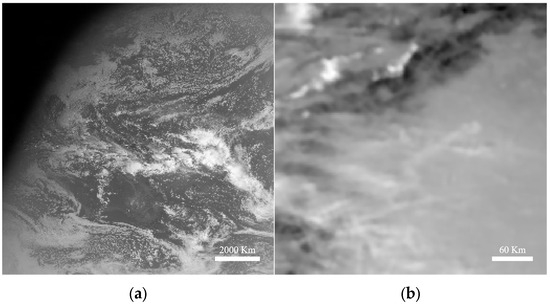
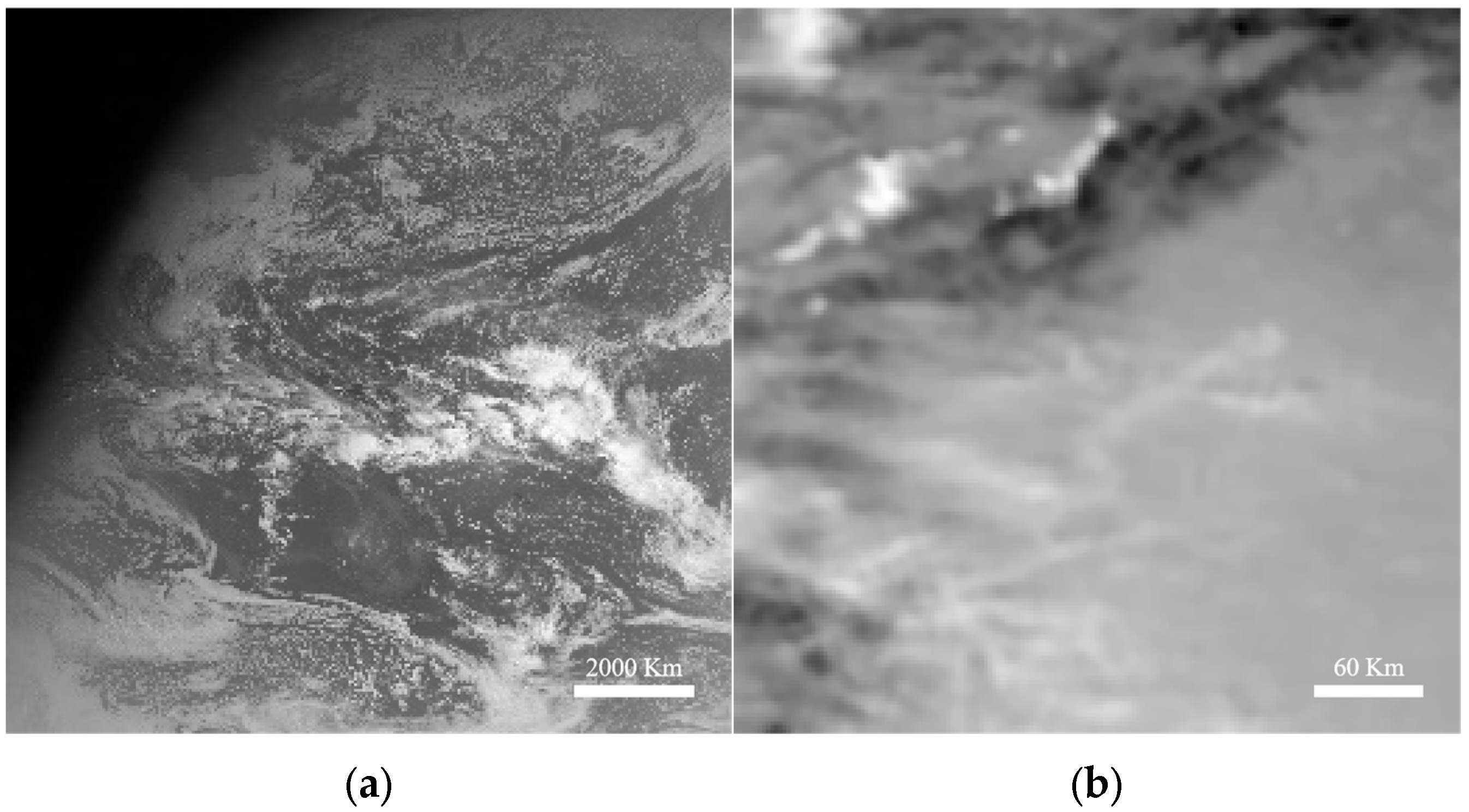
To improve processing efficiency and ensure the relevance of the selected cloud images, preprocessing is necessary. Assuming a cloud motion speed of 30 m/s [16] and a maximum prediction horizon of 2 h, a circular region covering a 200 km radius and centered around the target PV power station is selected as the prediction region, corresponding to a 200 × 200 pixel area. The cloud images are then normalized and geometrically corrected, as shown in Figure 1.

Figure 1. (a) Original image. (b) Preprocessed image.

2.2. Satellite Cloud Image Fusion

Different spectral channels provide different types of cloud information. In the visible bands, reflectance at three specific wavelengths is proportional to cloud optical thickness, allowing quantitative characterization of daytime cloud properties. In the near-infrared bands, reflectance indicates the cloud particle size distribution and effective radius. In the infrared bands, radiance information reflects cloud-top temperature, cloud-top height, and the associated water vapor distribution [17]. Therefore, integrating multispectral satellite cloud image data can significantly improve the prediction accuracy of cloud motion speed and direction.

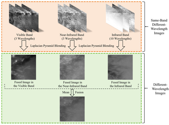
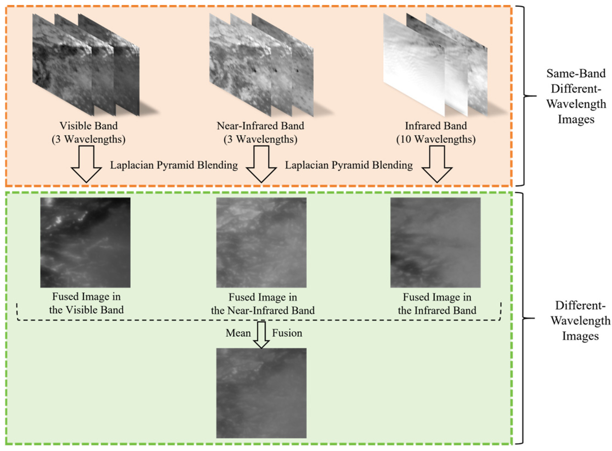
Because images at different wavelengths and in different spectral channels contain complementary information, image fusion is required. The Laplacian pyramid can capture detailed image features at different scales [18,19]. Therefore, Laplacian pyramid blending is used to fuse same-band images at different wavelengths, yielding fused images for the visible, near-infrared, and infrared bands. A mean fusion method is then applied to the three band-level fused images to obtain the final fused satellite cloud image. The core formulation of the Laplacian pyramid is given as follows:

$$\{\begin{array}{c}{\mathrm{L}}_{\mathrm{i}}={\mathrm{G}}_{\mathrm{i}}-{\mathrm{f}}_{\mathrm{U}\mathrm{S}}\left({\mathrm{G}}_{\mathrm{i}}\right)\\ {\mathrm{L}}_{\mathrm{N}}{=\mathrm{G}}_{\mathrm{N}}\end{array}$$

(1)

where ${\mathrm{L}}_{\mathrm{i}}$ denotes the Laplacian pyramid image at layer i, ${\mathrm{f}}_{\mathrm{U}\mathrm{S}}$ represents the up-sampling operation, and ${\mathrm{G}}_{\mathrm{N}}$ and ${\mathrm{L}}_{\mathrm{N}}$ denote the lowest-resolution layers of the Gaussian and Laplacian pyramids, respectively. The process of satellite cloud image fusion is shown in Figure 2.

Figure 2. Satellite image fusion process.

3. Extraction of Fused Predicted Cloud Features

3.1. Cloud Image Feature Extraction

3.1.1. Gray-Level Co-Occurrence Matrix

In satellite cloud images, different cloud types exhibit significant differences in texture characteristics because of their spatial distribution at different levels. For instance, cumulonimbus clouds typically exhibit strong gray-level variations and distinct edge structures, resulting in high contrast and high entropy, whereas stratiform clouds show a more uniform gray-level distribution, with high energy and homogeneity. The spatial dependency of gray-level variations in cloud layers can be captured through the Gray-Level Co-occurrence Matrix (GLCM) approach, which quantifies the spatial distribution characteristics associated with clouds through texture-related parameters. This offers reliable support for subsequent cloud characterization and forecasting and also supports cloud evolution analysis and solar irradiance prediction. The GLCM is a statistical method that describes image texture characteristics by analyzing pixel co-occurrence frequencies, and it has strong robustness [20].

Assume that pixel values range from [0, G − 1], where G represents the number of gray levels. For two pixels at positions $\left({\mathrm{a}}_{\mathrm{i}},{\mathrm{b}}_{\mathrm{i}}\right)$ and $\left({\mathrm{c}}_{\mathrm{j}},{\mathrm{d}}_{\mathrm{j}}\right)$ separated by a distance q in direction θ, the co-occurrence frequency is expressed as follows:

$$\mathrm{P}\left({\mathrm{i}}_{\mathrm{t}},{\mathrm{j}}_{\mathrm{t}},\mathrm{q},\mathsf{\theta }\right)=\mathrm{f}\left(\left({\mathrm{a}}_{\mathrm{i}},{\mathrm{b}}_{\mathrm{i}}\right),\left({\mathrm{c}}_{\mathrm{j}},{\mathrm{d}}_{\mathrm{j}}\right)\in \mathrm{I}|\mathrm{I}\left({\mathrm{c}}_{\mathrm{j}},{\mathrm{d}}_{\mathrm{j}}\right)={\mathrm{j}}_{\mathrm{t}}\right)$$

(2)

where ${\mathrm{i}}_{\mathrm{t}}$ and ${\mathrm{j}}_{\mathrm{t}}$ are the gray values of two pixels, and $\mathrm{P}\left({\mathrm{i}}_{\mathrm{t}},{\mathrm{j}}_{\mathrm{t}},\mathrm{q},\mathsf{\theta }\right)$ denotes the co-occurrence frequency under the given q and θ.

The original texture features extracted by the GLCM are usually transformed into statistical feature parameters through higher-order statistical processing, such as angular second moment (ASM), correlation (COR), and entropy (ENT). ASM reflects image uniformity and texture coarseness, COR measures the linear dependence between gray values, and ENT represents the randomness of the texture distribution. Their expressions are given as follows:

$$\{\begin{array}{c}\mathrm{ASM}={\displaystyle \sum _{{\mathrm{i}}_{\mathrm{t}},{\mathrm{j}}_{\mathrm{t}}}}{\mathrm{P}({\mathrm{i}}_{\mathrm{t}},{\mathrm{j}}_{\mathrm{t}})}^2\\ \mathrm{COR}={\displaystyle \frac{{\sum }_{{\mathrm{i}}_{\mathrm{t}},{\mathrm{j}}_{\mathrm{t}}}({\mathrm{i}}_{\mathrm{t}}-{\mathsf{\mu }}_{{\mathrm{i}}_{\mathrm{t}}})({\mathrm{j}}_{\mathrm{t}}-{\mathsf{\mu }}_{{\mathrm{j}}_{\mathrm{t}}})\mathrm{P}({\mathrm{i}}_{\mathrm{t}},{\mathrm{j}}_{\mathrm{t}})}{{\mathsf{\sigma }}_{{\mathrm{i}}_{\mathrm{t}}}{\mathsf{\sigma }}_{{\mathrm{j}}_{\mathrm{t}}}}}\\ \mathrm{ENT}={\displaystyle \sum _{{\mathrm{i}}_{\mathrm{t}}}}{\displaystyle \sum _{{\mathrm{j}}_{\mathrm{t}}}}\mathrm{P}({\mathrm{i}}_{\mathrm{t}},{\mathrm{j}}_{\mathrm{t}})\mathrm{l}\mathrm{g}\mathrm{P}({\mathrm{i}}_{\mathrm{t}},{\mathrm{j}}_{\mathrm{t}})\end{array}$$

(3)

where ${\mathsf{\mu }}_{{\mathrm{i}}_{\mathrm{t}}}$, ${\mathsf{\mu }}_{{\mathrm{j}}_{\mathrm{t}}}$ and ${\mathsf{\sigma }}_{{\mathrm{i}}_{\mathrm{t}}}$, ${\mathsf{\sigma }}_{{\mathrm{j}}_{\mathrm{t}}}$ denote the mean and standard deviation of gray values.

3.1.2. Discrete Wavelet Transform

Wavelet transform has long been used as an effective tool for multiresolution analysis, since it allows a signal to be examined at different scales through translation and dilation operations. For discrete signals in particular, the Discrete Wavelet Transform (DWT) offers strong time-frequency localization while retaining a sparse form of representation, which makes it well suited to time-series analysis. When applied to image feature extraction, it helps separate meaningful structural information from background interference and, at the same time, captures edge and texture characteristics more clearly. This is especially relevant for satellite cloud images, whose content is not only strongly nonstationary but also characterized by directional spatial patterns and evident spatiotemporal variability in cloud distribution. Under such conditions, DWT can describe the broad background of cloud layers as well as the finer details near their boundaries, so both coarse structural information and subtle cloud features can be preserved for subsequent PV power prediction [21,22]. The DWT can be expressed as follows:

$$\mathrm{X}({\mathrm{i}}_{\mathrm{t}},{\mathrm{j}}_{\mathrm{t}})=\sum _{{\mathrm{m}}_{\mathrm{t}}}\sum _{{\mathrm{n}}_{\mathrm{t}}}\mathrm{I}({\mathrm{m}}_{\mathrm{t}},{\mathrm{n}}_{\mathrm{t}})\mathsf{\phi }({\mathrm{i}}_{\mathrm{t}},{\mathrm{j}}_{\mathrm{t}},{\mathrm{m}}_{\mathrm{t}},{\mathrm{n}}_{\mathrm{t}})$$

(4)

where $\mathrm{I}({\mathrm{m}}_{\mathrm{t}},{\mathrm{n}}_{\mathrm{t}})$ is the original image, $\mathsf{\phi }({\mathrm{i}}_{\mathrm{t}},{\mathrm{j}}_{\mathrm{t}},{\mathrm{m}}_{\mathrm{t}},{\mathrm{n}}_{\mathrm{t}})$ is the wavelet basis function, and X(i, j) denotes the wavelet coefficients.

DWT decomposes an image into a low-frequency subband (LL), a horizontally oriented high-frequency subband (LH), and a vertically oriented high-frequency subband (HL). Higher-order statistical processing of these three components yields the corresponding statistical feature parameters. The standard deviation of LL (LL_std) reflects the overall brightness and texture, while the entropy of LH (LH_entropy) and HL (HL_entropy) reflect texture complexity in the horizontal and vertical directions, in that order. Their formulations are given below:

$$\{\begin{array}{c}\mathrm{L}{\mathrm{L}}_{\mathrm{s}\mathrm{t}\mathrm{d}}=\sqrt{{\displaystyle \frac{1}{\mathrm{M}\mathrm{N}}}{\displaystyle \sum _{{\mathrm{i}}_{\mathrm{t}}=1}^{\mathrm{M}}}{\displaystyle \sum _{{\mathrm{j}}_{\mathrm{t}}=1}^{\mathrm{N}}}{(\mathrm{L}\mathrm{L}\left({\mathrm{i}}_{\mathrm{t}},{\mathrm{j}}_{\mathrm{t}}\right)-\mathsf{\mu })}^2}\\ \mathrm{L}{\mathrm{H}}_{\mathrm{e}\mathrm{n}\mathrm{t}}=-{\displaystyle \sum _{{\mathrm{i}}_{\mathrm{t}}=1}^{\mathrm{M}}}{\displaystyle \sum _{{\mathrm{j}}_{\mathrm{t}}=1}^{\mathrm{N}}}\mathrm{L}\mathrm{H}\left({\mathrm{i}}_{\mathrm{t}},{\mathrm{j}}_{\mathrm{t}}\right){\mathrm{l}\mathrm{o}\mathrm{g}}_2\left|\mathrm{L}\mathrm{H}({\mathrm{i}}_{\mathrm{t}},{\mathrm{j}}_{\mathrm{t}})\right|\\ \mathrm{H}{\mathrm{L}}_{\mathrm{e}\mathrm{n}\mathrm{t}}=-{\displaystyle \sum _{{\mathrm{i}}_{\mathrm{t}}=1}^{\mathrm{M}}}{\displaystyle \sum _{{\mathrm{j}}_{\mathrm{t}}=1}^{\mathrm{N}}}\mathrm{H}\mathrm{L}\left({\mathrm{i}}_{\mathrm{t}},{\mathrm{j}}_{\mathrm{t}}\right){\mathrm{l}\mathrm{o}\mathrm{g}}_2\left|\mathrm{H}\mathrm{L}{\mathrm{i}}_{\mathrm{t}},{\mathrm{j}}_{\mathrm{t}})\right|\end{array}$$

(5)

where M and N denote the dimensions of the component, and μ denotes the mean value.

The joint use of GLCM and wavelet transform was chosen for more than computational convenience. An equally important reason is that the two methods offer cloud representations with clear physical meaning. GLCM features are useful for characterizing texture attributes, including uniformity, contrast, and irregularity, whereas wavelet-based features are better suited to describing multiscale and nonstationary patterns in satellite cloud images. When the number of samples is limited, these handcrafted descriptors still tend to remain relatively stable, and they can reflect cloud morphological properties that are closely associated with solar radiation attenuation. By comparison, relying only on deep feature extraction often demands a larger amount of training data, while the resulting features are usually less straightforward to interpret from a physical perspective. Therefore, in this study, GLCM and wavelet transform are used to characterize cloud structure, while deep models are mainly employed for feature prediction, feature interaction, and temporal dependency modeling.

3.2. Predicted Cloud Feature Extraction

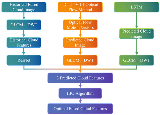
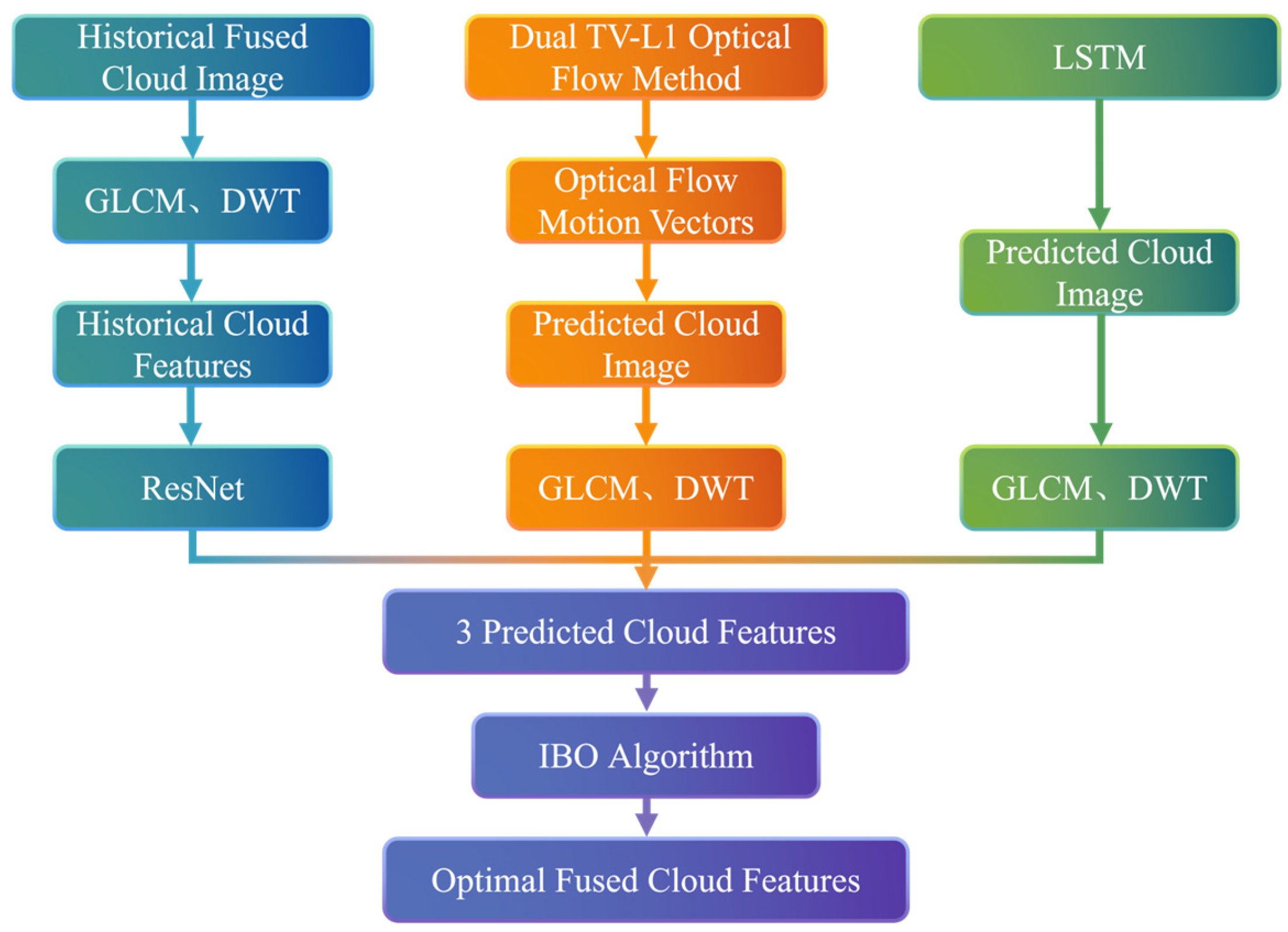
Based on the residual network, the optical flow method, and the long short-term memory (LSTM) network, three types of predicted cloud image features at future time steps are obtained. The first method performs prediction using only historical cloud image feature variables, while the other two methods predict future cloud images based on optical flow vectors and deep learning, respectively. The corresponding cloud image features are subsequently extracted from the predicted images. Finally, the improved Bayesian Optimization (BO) algorithm is used to obtain the optimal predicted cloud features, thereby enhancing the correlation between the cloud image features and PV power. The specific procedure is shown in Figure 3.

Figure 3. Optimal Fused Cloud Image Feature Flowchart.

3.2.1. Residual Network

Historical cloud features are derived from the Gray-Level Co-occurrence Matrix (GLCM) together with the discrete wavelet transform (DWT), while the residual network (ResNet) is used to predict future cloud features. ResNet introduces identity mappings to alleviate gradient vanishing and improve forward information propagation [23]. The basic residual block of ResNet can be expressed as follows:

$$\mathrm{y}=\mathrm{M}\left(\mathrm{x},\left\{{\mathrm{W}}_{\mathrm{i}}\right\}\right)+\mathrm{x}$$

(6)

Here, x is the input of the previous layer, $\mathrm{M}\left(\mathrm{x},\left\{{\mathrm{W}}_{\mathrm{i}}\right\}\right)$ denotes the output after convolution and activation, and y is the residual output.

3.2.2. Dual TV-L1 Optical Flow Method

Optical flow describes the instantaneous motion of pixels between adjacent frames and is widely used for cloud image prediction. For satellite cloud images, it assumes that cloud gray levels remain approximately constant over a short time and estimates pixel displacement to obtain the corresponding motion vector field, thereby characterizing cloud motion between consecutive images [24]. In this study, the Dual TV-L1 optical flow method is used to generate future cloud maps from adjacent satellite images. The resulting motion vectors are not directly input into the final PV forecasting model; instead, texture and wavelet features are extracted from the predicted cloud maps and included in the multidimensional predicted cloud feature set. Thus, cloud motion information is incorporated into the forecasting framework indirectly through future cloud structure representation. Assuming brightness constancy across two consecutive frames, the corresponding optical-flow constraint relation is expressed as

$$\{\begin{array}{c}\mathrm{I}\left({\mathrm{x}}_{\mathrm{i}},{\mathrm{y}}_{\mathrm{j}},{\mathrm{t}}_{\mathrm{k}}\right)=\mathrm{I}({\mathrm{x}}_{\mathrm{i}}+\mathrm{u},{\mathrm{y}}_{\mathrm{j}}+\mathrm{v},{\mathrm{t}}_{\mathrm{k}}+1)\\ {\mathrm{I}}_{\mathrm{x}}\mathrm{u}+{\mathrm{I}}_{\mathrm{y}}\mathrm{v}+{\mathrm{I}}_{\mathrm{t}}=0\end{array}$$

(7)

where $\mathrm{I}\left({\mathrm{x}}_{\mathrm{i}},{\mathrm{y}}_{\mathrm{j}},{\mathrm{t}}_{\mathrm{k}}\right)$ denotes the pixel brightness at time t; u and v are the horizontal and vertical motion components; and ${\mathrm{I}}_{\mathrm{x}}$, ${\mathrm{I}}_{\mathrm{y}}$, and ${\mathrm{I}}_{\mathrm{t}}$ denote the spatial and temporal gradients.

To improve robustness, total variation (TV) regularization and the L1 norm are introduced to reduce image noise and enforce image smoothness [25]:

$$\{\begin{array}{c}\int \left({\left(\nabla \mathrm{u}\right)}^2+{\left(\nabla \mathrm{v}\right)}^2\right)\mathrm{d}\mathrm{x}\mathrm{d}\mathrm{y}\\ \int \left(\left|\mathrm{u}\right|+\left|\mathrm{v}\right|\right)\mathrm{d}\mathrm{x}\mathrm{d}\mathrm{y}\end{array}$$

(8)

where $\nabla \mathrm{u}$ and $\nabla \mathrm{v}$ denote the gradients of the optical flow fields u and v.

A dual optimization (Dual) technique is incorporated to reduce the discrepancy between predicted and reference images [26]. The forward and backward optical flow optimization expressions can be written as follows:

$$\{\begin{array}{c}\begin{array}{c}\mathrm{m}\mathrm{i}\mathrm{n}(\mathsf{\alpha },\mathsf{\beta },\mathsf{\gamma })\\ \mathsf{\alpha }=\int ({\left(\nabla \mathrm{u}\right)}^2+{\left(\nabla \mathrm{v}\right)}^2)\mathrm{d}\mathrm{x}\mathrm{d}\mathrm{y}\end{array}\\ \begin{array}{c}\mathsf{\beta }=\mathsf{\epsilon }\left(\left|\mathrm{u}\right|+\left|\mathrm{v}\right|\right)\\ \mathsf{\gamma }=\mathsf{ϵ}\int (\left|{\mathrm{u}}_{\mathrm{t}+1}-{\mathrm{u}}_{\mathrm{t}}\right|+\left|{\mathrm{v}}_{\mathrm{t}+1}-{\mathrm{v}}_{\mathrm{t}}\right|)\mathrm{d}\mathrm{x}\mathrm{d}\mathrm{y}\end{array}\end{array}$$

(9)

where $\mathsf{\epsilon }$ and $\mathsf{ϵ}$ are regularization parameters, and $\mathsf{\alpha }$, $\mathsf{\beta }$, and $\mathsf{\gamma }$ denote the constraint terms.

Using Equations (7)–(9), future satellite cloud images can be predicted, after which the corresponding cloud features are extracted with the proposed feature extraction method. These features then serve as the input for the subsequent feature fusion stage.

3.2.3. Long Short-Term Memory (LSTM)

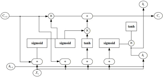
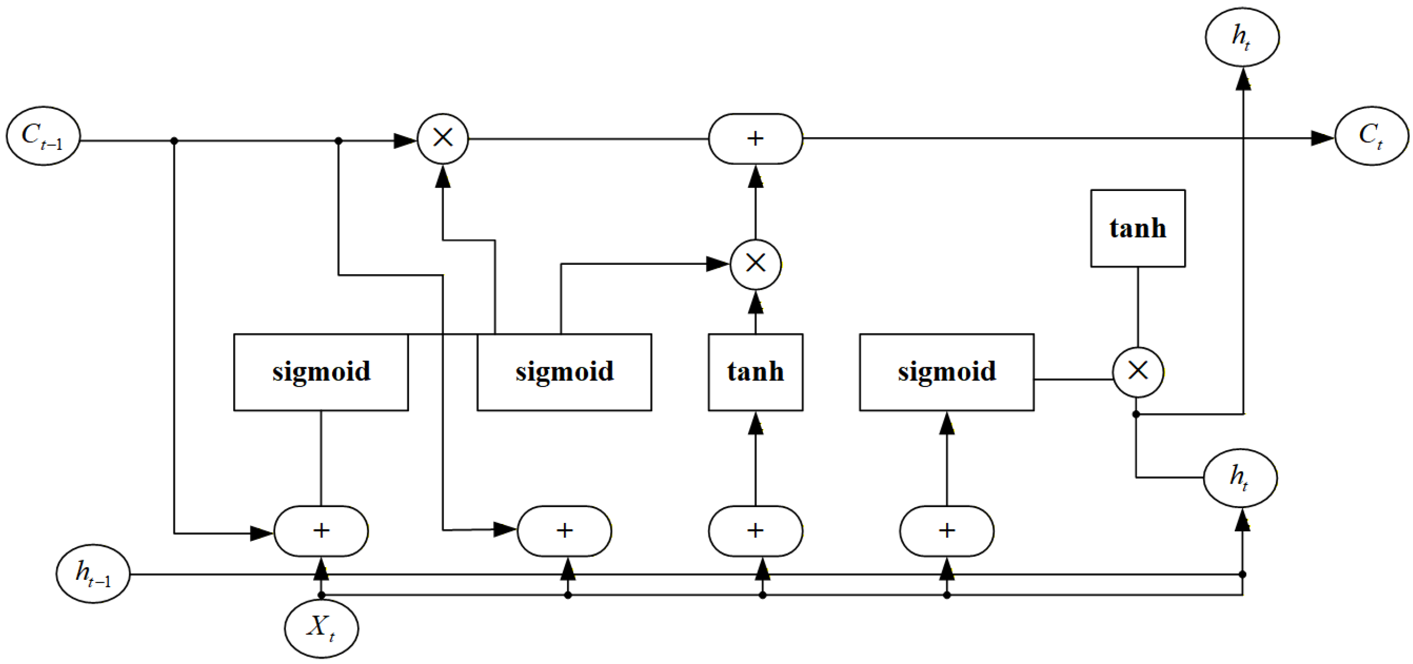
The core structure of the LSTM architecture is composed of three control gates, namely the forget gate, the input gate, and the output gate. The three gates selectively retain or discard information, enabling effective prediction of time-series data [27]. The network architecture is illustrated in Figure 4.

Figure 4. Long short-term memory neural network.

For the original input data x = (x₁, x₂, …, xₙ), the core computations of the LSTM are expressed as

$$\{\begin{array}{c}\begin{array}{c}{\mathrm{f}}_{\mathrm{t}}={\mathsf{\sigma }}_{\mathrm{t}}({\mathrm{G}}_{\mathrm{f}}\left[{\mathrm{y}}_{\mathrm{t}-1},{\mathrm{x}}_{\mathrm{t}}\right]+{\mathrm{m}}_{{\mathrm{f}}_{\mathrm{t}}})\\ {\mathrm{i}}_{\mathrm{t}}={\mathsf{\sigma }}_{\mathrm{t}}({{\mathrm{G}}_{\mathrm{f}}}_{\mathrm{i}}\left[{\mathrm{y}}_{\mathrm{t}-1},{\mathrm{x}}_{\mathrm{t}}\right]+{\mathrm{m}}_{{\mathrm{i}}_{\mathrm{t}}})\\ {\tilde{\mathrm{C}}}_{\mathrm{t}}=\mathrm{t}\mathrm{a}\mathrm{n}\mathrm{h}({{\mathrm{G}}_{\mathrm{f}}}_{\mathrm{c}}\left[{\mathrm{y}}_{\mathrm{t}-1},{\mathrm{x}}_{\mathrm{t}}\right]+{\mathrm{m}}_{\mathrm{c}})\end{array}\\ \begin{array}{c}{\mathrm{C}}_{\mathrm{t}}={\mathrm{f}}_{\mathrm{t}}{\mathrm{C}}_{\mathrm{t}-1}+{\mathrm{i}}_{\mathrm{t}}{\tilde{\mathrm{C}}}_{\mathrm{t}}\\ {\mathrm{o}}_{\mathrm{t}}={\mathsf{\sigma }}_{\mathrm{t}}({{\mathrm{G}}_{\mathrm{f}}}_{\mathrm{o}}\left[{\mathrm{y}}_{\mathrm{t}-1},{\mathrm{x}}_{\mathrm{t}}\right]+{\mathrm{m}}_{{\mathrm{o}}_{\mathrm{t}}})\\ {\mathrm{y}}_{\mathrm{t}}={\mathrm{o}}_{\mathrm{t}}{\tanh }_{\mathrm{t}}\left({\mathrm{C}}_{\mathrm{t}}\right)\end{array}\end{array}$$

(10)

Here, ${\mathrm{f}}_{\mathrm{t}}$, ${\mathrm{i}}_{\mathrm{t}}$, and ${\mathrm{o}}_{\mathrm{t}}$ denote the outputs of the forget gate, input gate, and output gate, respectively; ${\mathrm{y}}_{\mathrm{t}}$ represents the hidden state at time t; G and m denote the weight matrices and bias vectors, respectively; and ${\mathsf{\sigma }}_{\mathrm{t}}$ and ${\mathrm{t}\mathrm{a}\mathrm{n}\mathrm{h}}_{\mathrm{t}}$ denote a sigmoid nonlinear activation and a hyperbolic tangent nonlinear activation, in corresponding order.

By inputting the original satellite cloud image sequence data into the LSTM network and applying Equation (10), future cloud images can be predicted, and the corresponding cloud image features at future time steps can be extracted.

3.3. Improved Bayesian Optimization (BO) Algorithm

The BO algorithm [28] builds a proxy model for approximating the objective function on the basis of the evaluated objective values. The overall procedure is as follows.

Given a set of observations $\mathrm{X}=({\mathrm{x}}_1,{\mathrm{x}}_2,\dots ,{\mathrm{x}}_{\mathrm{n}})$ and the corresponding objective function values $\mathrm{Y}=({\mathrm{y}}_1,{\mathrm{y}}_2,\dots ,{\mathrm{y}}_{\mathrm{n}})$, a Gaussian process is employed to predict the function value at an unobserved sample point, which can be expressed as follows:

$$\{\begin{array}{c}\mathrm{M}\left(\mathrm{X},\mathrm{Y}\right)=\left[\begin{array}{ccc}\mathrm{m}({\mathrm{x}}_1,{\mathrm{x}}_1)& \dots & \mathrm{m}({\mathrm{x}}_1,{\mathrm{x}}_{\mathrm{n}})\\ ⋮& \ddots & ⋮\\ \mathrm{m}({\mathrm{x}}_{\mathrm{n}},{\mathrm{x}}_1)& \dots & \mathrm{m}({\mathrm{x}}_{\mathrm{n}},{\mathrm{x}}_{\mathrm{n}})\end{array}\right]\\ {\mathrm{m}}_{\ast }=\left[\begin{array}{c}\begin{array}{c}\mathrm{m}({\mathrm{x}}_{\ast },{\mathrm{x}}_1)\\ \mathrm{m}({\mathrm{x}}_{\ast },{\mathrm{x}}_2)\end{array}\\ ⋮\\ \mathrm{m}({\mathrm{x}}_{\ast },{\mathrm{x}}_{\mathrm{n}})\end{array}\right]\\ {\mathrm{m}}_{\ast \ast }=m({\mathrm{x}}_{\ast },{\mathrm{x}}_{\ast })\end{array}$$

(11)

where $\mathrm{M}\left(\mathrm{X},\mathrm{Y}\right)$ denotes the covariance matrix associated with the training samples, ${\mathrm{m}}_{\ast }$ represents the covariance vector linking the prediction point to the training samples, and ${\mathrm{m}}_{\ast \ast }$ denotes the autocovariance at the prediction point.

The prediction result of Gaussian process regression follows a Gaussian distribution with predictive mean ${\mathsf{\mu }}_{\mathrm{t}}$ and predictive variance ${\mathsf{\sigma }}_{\mathrm{t}}^2$, which can be expressed as follows:

$$\{\begin{array}{c}{\mathsf{\mu }}_{\mathrm{t}}={{\mathrm{m}}_{\ast }}^{\mathrm{T}}{[\mathrm{M}\left(\mathrm{X},\mathrm{Y}\right)+{\mathsf{\sigma }}_{\mathrm{n}}^2\mathrm{I}]}^{-1}y\\ {\mathsf{\sigma }}_{\mathrm{t}}^2={{{\mathrm{m}}_{\ast \ast }-\mathrm{m}}_{\ast }}^{\mathrm{T}}{[\mathrm{M}\left(\mathrm{X},\mathrm{Y}\right)+{\mathsf{\sigma }}_{\mathrm{n}}^2\mathrm{I}]}^{-1}{\mathrm{m}}_{\ast }\end{array}$$

(12)

where ${\mathsf{\sigma }}_{\mathrm{n}}^2$ denotes the noise variance, and I denotes the identity matrix.

The expected improvement (EI) acquisition function is adopted to guide the selection of the next sampling point in the hyperparameter search space. Its formulation can be expressed as follows:

$$\mathrm{E}\mathrm{I}\left({\mathrm{x}}_{\mathrm{t}}\right)=\left({\mathsf{\mu }}_{\mathrm{i}}\left({\mathrm{x}}_{\mathrm{t}}\right)-{\mathrm{y}}_{\mathrm{m}\mathrm{a}\mathrm{x}}\right){\mathsf{\phi }}_{\mathrm{i}}\left({\mathrm{Z}}_{\mathrm{t}}\right)+{\mathsf{\sigma }}_{\mathrm{i}}\left({\mathrm{x}}_{\mathrm{t}}\right){\mathsf{\omega }}_{\mathrm{i}}\left({\mathrm{Z}}_{\mathrm{t}}\right)$$

(13)

where ${\mathsf{\mu }}_{\mathrm{i}}\left({\mathrm{x}}_{\mathrm{t}}\right)$ and ${\mathsf{\sigma }}_{\mathrm{i}}\left({\mathrm{x}}_{\mathrm{t}}\right)$ represent the predictive mean and predictive standard deviation of the Gaussian process at point x, respectively; ${\mathrm{y}}_{\mathrm{m}\mathrm{a}\mathrm{x}}$ denotes the current best observed objective value; ${\mathrm{Z}}_{\mathrm{t}}={\displaystyle \frac{{\mathsf{\mu }}_{\mathrm{i}}\left({\mathrm{x}}_{\mathrm{t}}\right)-{\mathrm{y}}_{\mathrm{m}\mathrm{a}\mathrm{x}}}{{\mathsf{\sigma }}_{\mathrm{i}}\left({\mathrm{x}}_{\mathrm{t}}\right)}}$ represents the normalized improvement; and ${\mathsf{\phi }}_{\mathrm{i}}\left({\mathrm{Z}}_{\mathrm{t}}\right)$ and ${\mathsf{\omega }}_{\mathrm{i}}\left({\mathrm{Z}}_{\mathrm{t}}\right)$ denote the standard normal cumulative distribution and its probability density, respectively.

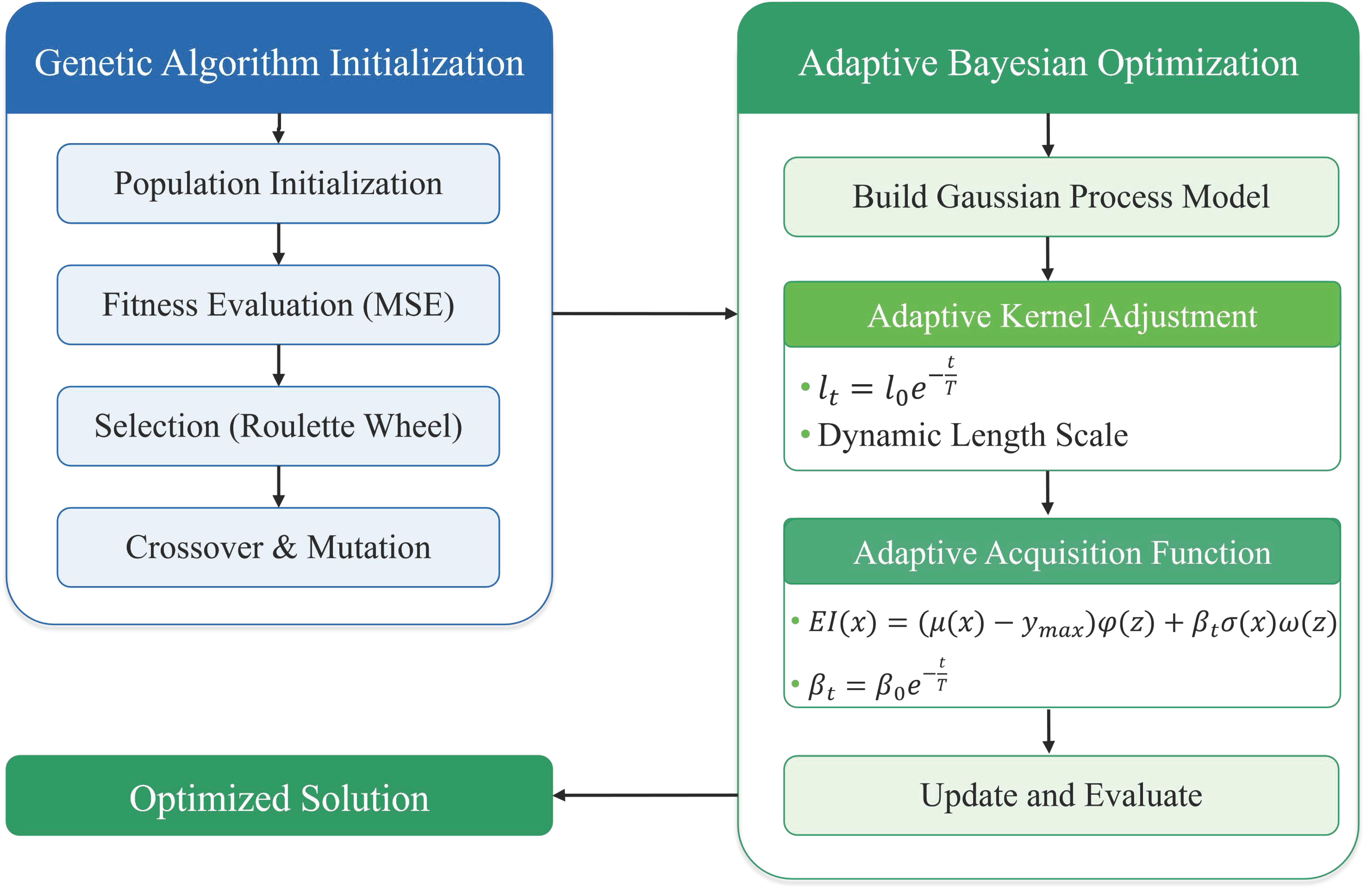
Within the conventional Bayesian Optimization (BO) framework, Gaussian Process Regression (GPR) serves as a surrogate for the objective function, while the acquisition function is responsible for choosing the next sample to evaluate. This setting works well in many optimization tasks, but once the search space becomes larger and the problem itself more involved, the search may settle too early around a local optimum. In view of this limitation, an improved Bayesian Optimization (IBO) algorithm is adopted in this study, and its pseudocode is presented in Algorithm 1. Instead of relying on BO alone from the beginning, the proposed strategy first makes use of the global search ability of the Genetic Algorithm (GA) to provide a more favorable starting solution. During the subsequent search, the BO procedure is further refined through an adaptive scheme in which the kernel and acquisition functions are adjusted as the iterations proceed, allowing exploration and exploitation to be balanced in a more flexible manner. The overall optimization workflow is shown in Figure 5.

Figure 5. Flowchart of the improved Bayesian optimization algorithm.

To lower the possibility of premature convergence, GA is introduced at the initial stage to explore the feature-weight space more broadly. A population is first generated and evaluated with the fitness function, after which individuals are selected according to roulette-wheel probabilities derived from their fitness values. Offspring are then produced through arithmetic crossover between parent individuals, whereas mutation is retained to keep the population from becoming overly uniform during evolution. As these operations are repeated, the feature weights are gradually improved until a GA-based solution is obtained. The promising solutions found in this stage are then passed to BO as initial seeds, which gives the subsequent search a stronger starting region and broader coverage of the search space. As a result, the later local optimization can proceed with better efficiency and more stable convergence. An adaptive Bayesian Optimization strategy is further introduced, with a dynamic adjustment mechanism for the kernel function. As the algorithm progresses, the length scale of the kernel function gradually decreases, allowing the algorithm to focus more on local regions, as described by the following expression:

$$\{\begin{array}{c}k\left(\mathrm{x},{\mathrm{x}}^{\prime }\right)=C\left(\mathrm{1,0}\right)\mathrm{RBF}\left({\mathrm{l}}_{\mathrm{t}}\right)\\ {\mathrm{l}}_{\mathrm{t}}={\mathrm{l}}_0{\mathrm{e}}^{-{\displaystyle \frac{\mathrm{t}}{\mathrm{T}}}}\end{array}$$

(14)

where ${\mathrm{l}}_0$ denotes the initial length scale, and t and T represent the current and maximum numbers of iterations, respectively.

Since the choice of the acquisition function affects the efficiency of the BO algorithm, an adaptive function is introduced to dynamically adjust the exploration factor. During the optimization process, the dependence on exploration gradually decreases, which helps balance exploration and exploitation and makes the search focus more on local optima. The specific mathematical formulation is given by the following expression:

$$\{\begin{array}{c}\mathrm{EI}\left(\mathrm{x}\right)=\left(\mathsf{\mu }\left(\mathrm{x}\right)-{\mathrm{y}}_{\mathrm{m}\mathrm{a}\mathrm{x}}\right)\mathsf{\phi }\left(\mathrm{Z}\right)+{\mathsf{\beta }}_{\mathrm{t}}\mathsf{\sigma }\left(\mathrm{x}\right)\mathsf{\omega }\left(\mathrm{Z}\right)\\ {\mathsf{\beta }}_{\mathrm{t}}={\mathsf{\beta }}_0{\mathrm{e}}^{-{\displaystyle \frac{\mathrm{t}}{\mathrm{T}}}}\end{array}$$

(15)

where ${\mathsf{\beta }}_0$ denotes the initial exploration factor.

Using the improved BO (IBO) algorithm to optimize the three predicted cloud image features mentioned above, the corresponding feature weights ${\mathsf{\omega }}_1,{\mathsf{\omega }}_2,{\mathsf{\omega }}_3$ are obtained. The final fused cloud image feature ${\widehat{\mathrm{y}}}_{\mathrm{i}}$ is calculated using the optimized weights and can be expressed as follows:

$${\widehat{\mathrm{y}}}_{\mathrm{i}}={\displaystyle \frac{{\mathsf{\omega }}_1}{{\mathsf{\omega }}_1+{\mathsf{\omega }}_2+{\mathsf{\omega }}_3}}{\mathrm{x}}_{\mathrm{i}1}+{\displaystyle \frac{{\mathsf{\omega }}_2}{{\mathsf{\omega }}_1+{\mathsf{\omega }}_2+{\mathsf{\omega }}_3}}{\mathrm{x}}_{\mathrm{i}2}+{\displaystyle \frac{{\mathsf{\omega }}_3}{{\mathsf{\omega }}_1+{\mathsf{\omega }}_2+{\mathsf{\omega }}_3}}{\mathrm{x}}_{\mathrm{i}3}$$

(16)

where ${\mathrm{x}}_{\mathrm{i}1}$, ${\mathrm{x}}_{\mathrm{i}2}$, and ${\mathrm{x}}_{\mathrm{i}3}$ denote the extracted cloud image feature values.

Algorithm 1. Pseudocode of the IBO
Input	pop_size—Population size num_generations—Maximum generations mutation_rate—Mutation rate X, y—Input features and target
1	population ← initialize_population(pop_size, dim)
2	for generation = 1 to num_generations do
3	fitness_values ← compute fitness of each individual
4	selected ← selection(population, fitness_values)
5	new_population ← {}
6	for i = 1 to length(selected) step 2 do
7	p1, p2 ← selected[i], selected[i+1]
8	c1, c2 ← crossover(p1, p2)
9	c1 ← mutate(c1, mutation_rate)
10	c2 ← mutate(c2, mutation_rate)
11	new_population ← new_population ∪ {c1, c2}
12	end for
13	population ← new_population
14	end for
15	best_ga_weights ← argmin(fitness(ind, X, y)) for ind in population
16	X_init ← {best_ga_weights}
17	y_init ← {fitness(best_ga_weights, X, y)}
18	for iteration = 1 to n_iter do
19	kernel ← adaptive_kernel(iteration)
20	gp ← GaussianProcessRegressor(kernel = kernel, n_restarts_optimizer = 10, alpha = 1 × 10−2)
21	gp.fit(X_init, y_init)
22	next_point ← random_uniform(0, 1, X.shape [1])
23	max_acquisition ← -infinity
24	for _ in range(100) do
25	candidate ← random_uniform(0, 1, X.shape [1])
26	acq_value ← adaptive_acquisition(candidate, gp)
27	if acq_value > max_acquisition then
28	max_acquisition ← acq_value
29	next_point ← candidate
30	end if
31	end for
32	new_fitness ← fitness(next_point, X, y)
33	X_init ← concatenate(X_init, next_point)
34	y_init ← append(y_init, new_fitness)
35	print(f”Iteration {iteration + 1}, Best Fitness: {new_fitness}”)
36	end for
Output	Best weights—Optimal feature weights

The dynamic adjustment of cloud image feature weights through the IBO algorithm automatically optimizes the relative importance of different cloud image features. This process enables a more accurate representation of the contribution of each feature and better reflects the dynamic changes in cloud layers. As a result, the model becomes more sensitive to critical cloud-layer features. By feeding the fused cloud image features into the subsequent PV power prediction model, the impact of cloud layers on solar output can be captured more effectively, thereby improving the overall prediction accuracy and efficiency.

4. Hybrid Neural Network Prediction Model

4.1. Convolutional Neural Network

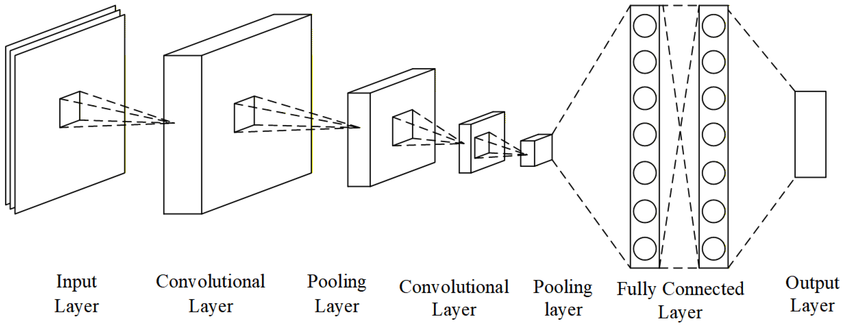
The CNN-LSTM model integrates the strengths of convolutional neural networks (CNNs) for learning spatial representations with the capability of LSTM networks in time-series modeling [29]. The LSTM network was introduced in the previous section. CNNs learn spatial representations from the input sequence via convolution operations and use dense layers for classification or regression tasks. A standard CNN framework is generally composed of an input layer, convolution blocks, pooling modules, dense layers, and an output layer [30], as shown in Figure 6.

Figure 6. Convolutional neural network structure.

In this study, the model takes time-series data as input, while the convolution operation can be expressed as follows:

$$\{\begin{array}{c}{\mathrm{Y}}_{\mathrm{t}}={\displaystyle \sum _{\mathrm{i}=0}^{\mathrm{k}-1}}{\mathrm{x}}_{\mathrm{t}+\mathrm{i}}{\mathsf{\omega }}_{\mathrm{i}}+\mathrm{b}\\ \mathrm{ReLU}\left(\mathrm{z}\right)=\max (0,z)\\ {\mathrm{Y}}_{\mathrm{m}}=\max \left({\mathrm{x}}_{\mathrm{t}+1},{\mathrm{x}}_{\mathrm{t}+2},\dots ,{\mathrm{x}}_{\mathrm{t}+\mathrm{p}-1}\right)\end{array}$$

(17)

Here, ${\mathrm{Y}}_{\mathrm{t}}$ denotes the convolution output, ${\mathrm{x}}_{\mathrm{t}}$ represents the time-series input data, ${\mathsf{\omega }}_{\mathrm{i}}$ denotes the convolution kernel weights, and b denotes a bias parameter. ReLU serves as a nonlinear activation mechanism that introduces nonlinearity and helps reduce computational complexity. ${\mathrm{Y}}_{\mathrm{m}}$ denotes the pooling output.

4.2. Multi-Head Self-Attention Mechanism

The MSA consists of multiple parallel self-attention units that attend to different feature subspaces simultaneously. This mechanism allows the model to emphasize critical content while filtering out redundant signals, thereby enhancing feature diversity and global representation capability [31]. The specific procedure is described as follows:

(1)

The input sequence undergoes linear mapping to form the query (${\mathrm{Q}}_{\mathrm{t}}$), key (${\mathrm{K}}_{\mathrm{t}}$), and value (${\mathrm{V}}_{\mathrm{t}}$) matrices. Multiple attention heads are used to project the input into different feature subspaces. The corresponding formulation can be expressed as follows:

$$\{\begin{array}{c}\mathrm{Attention}\left({\mathrm{Q}}_{\mathrm{t}},{\mathrm{K}}_{\mathrm{t}},{\mathrm{V}}_{\mathrm{t}}\right)=\mathrm{softmax}\left({\displaystyle \frac{{\mathrm{Q}}_{\mathrm{t}}{{\mathrm{K}}_{\mathrm{t}}}^{\mathrm{T}}}{\sqrt{{\mathrm{d}}_{\mathrm{k}}}}}\right){\mathrm{V}}_{\mathrm{t}}\\ \mathrm{MSA}\left(\mathrm{X}\right)=\mathrm{Concat}({\mathrm{h}\mathrm{e}\mathrm{a}\mathrm{d}}_1,{\mathrm{h}\mathrm{e}\mathrm{a}\mathrm{d}}_2,\dots ,{\mathrm{h}\mathrm{e}\mathrm{a}\mathrm{d}}_{\mathrm{h}}){\mathrm{W}}^{\mathrm{O}}\end{array}$$

(18)

Here, ${\mathrm{Q}}_{\mathrm{t}}$, ${\mathrm{K}}_{\mathrm{t}}$, and ${\mathrm{V}}_{\mathrm{t}}$ denote the matrices corresponding to queries, keys, and values, in sequence; ${\mathrm{d}}_{\mathrm{k}}$ represents the dimensionality of the key vectors; softmax serves to calculate attention coefficients; ${\mathrm{h}\mathrm{e}\mathrm{a}\mathrm{d}}_{\mathrm{i}}=(\mathrm{X}{\mathrm{W}}_{\mathrm{i}}^{{\mathrm{Q}}_{\mathrm{t}}},\mathrm{X}{\mathrm{W}}_{\mathrm{i}}^{{\mathrm{K}}_{\mathrm{t}}},\mathrm{X}{\mathrm{W}}_{\mathrm{i}}^{{\mathrm{V}}_{\mathrm{t}}})$ denotes the input mapped to the i-th attention branch; ${\mathrm{W}}_{\mathrm{i}}^{{\mathrm{Q}}_{\mathrm{t}}}$, ${\mathrm{W}}_{\mathrm{i}}^{{\mathrm{K}}_{\mathrm{t}}}$, and ${\mathrm{W}}_{\mathrm{i}}^{{\mathrm{V}}_{\mathrm{t}}}$ correspond to the projection matrices associated with that head; and ${\mathrm{W}}^{\mathrm{O}}$ denotes the final projection matrix at the output stage.

(2)

Through multiple self-attention operations, each attention head learns independently in a different projected subspace. The results produced by each attention head are subsequently merged and passed through a linear mapping back into the original feature dimension to obtain the final multi-head attention output.

4.3. CNN-MSA-LSTM Model

The core idea of the CNN–LSTM model is to use a convolutional neural network (CNN) to extract local features and then feed the resulting feature sequences into an LSTM network for global dependency learning and temporal modeling. However, from the perspective of information propagation, the conventional CNN–LSTM architecture has certain theoretical limitations.

First, the representation ability provided by CNN convolutional layers remains constrained by the size of the convolution kernels, so feature extraction is limited to local neighborhood information. Second, after convolution, the output feature variables are directly passed to the LSTM without explicit modeling of global correlations. The dependencies among different time steps rely entirely on the implicit learning of the gating mechanism within the LSTM, which may reduce the efficiency of long-range dependency modeling.

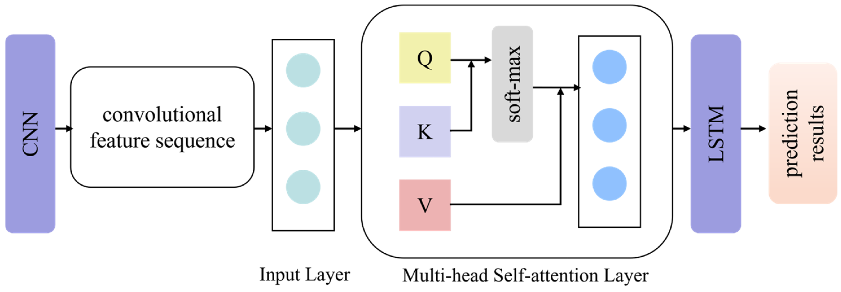
To address these limitations, a Multi-Head Self-Attention (MSA) module is introduced between the CNN and LSTM modules. The MSA mechanism reconstructs the global dependencies of the fused cloud image features and meteorological features while preserving temporal order information, thereby improving prediction accuracy and computational efficiency. The overall architecture of the CNN–MSA–LSTM model is illustrated in Figure 7.

Figure 7. Structure of the CNN–MSA–LSTM model.

First, the CNN is employed to perform local feature extraction from the input feature sequences, thereby obtaining a feature matrix. The feature matrix is then fed into the MSA module for global dependency reconstruction. With the aid of the multi-head attention module, feature representations are projected onto several subspaces to construct multiple groups of correlated feature matrices. Finally, the reconstructed feature matrix is input into the LSTM network for temporal modeling, and the prediction results are generated.

Compared with the conventional CNN–LSTM model and the LSTM model equipped with a single attention mechanism, the proposed model has the following advantages:

(1)

Relative to the traditional CNN–LSTM architecture, the proposed CNN–MSA–LSTM framework forms a hierarchical framework of “local feature extraction–global correlation reconstruction–temporal dynamic modeling.” This framework enables cross-temporal association of multiscale feature information and promotes the transition of feature representation from local modeling to global modeling. Consequently, it provides stronger representation capability and higher prediction stability for photovoltaic power forecasting with multidimensional feature inputs.

(2)

Compared with an LSTM that relies on only one attention mechanism, the MSA module handles cloud image information, meteorological dynamics, and historical power variations through several attention heads working in different feature subspaces. This makes it possible to model these heterogeneous signals from multiple perspectives before combining them again within a unified representation. When meteorological conditions become more complicated, such a design can reduce the tendency of single-head attention to place too much emphasis on a limited set of features, while also giving the model greater room to capture richer patterns in the data.

4.4. Overfitting Suppression

To prevent overfitting in the neural network model, the Dropout technique is employed by randomly deactivating a portion of neurons during training, so that a different subnetwork is formed at each iteration. Meanwhile, the RAdam optimization algorithm is adopted to improve the generalization capability and convergence stability of the model. The main steps are as follows [32]:

Gradient-based first- and second-order moment estimates are calculated to construct an adaptive update direction. Bias correction is then applied to both moment estimates to eliminate the effect of the large bias introduced during the early iterations.

A rectification factor is introduced to adaptively assess the trustworthiness of the step size from the current update index together with the bias magnitude associated with the second-moment estimate. The corresponding formulation can be expressed as follows:

$$\{\begin{array}{c}{\mathsf{\rho }}_{\mathrm{t}}={\mathsf{\rho }}_{\mathrm{\infty }}-{\displaystyle \frac{2\mathrm{t}{\mathsf{\beta }}^{\mathrm{t}}}{1-{\mathsf{\beta }}^{\mathrm{t}}}}\\ {\mathsf{\rho }}_{\mathrm{\infty }}={\displaystyle \frac{2}{1-\mathsf{\beta }}}-1\end{array}$$

(19)

4.5. Prediction Model Based on IBO-CNN-MSA-LSTM

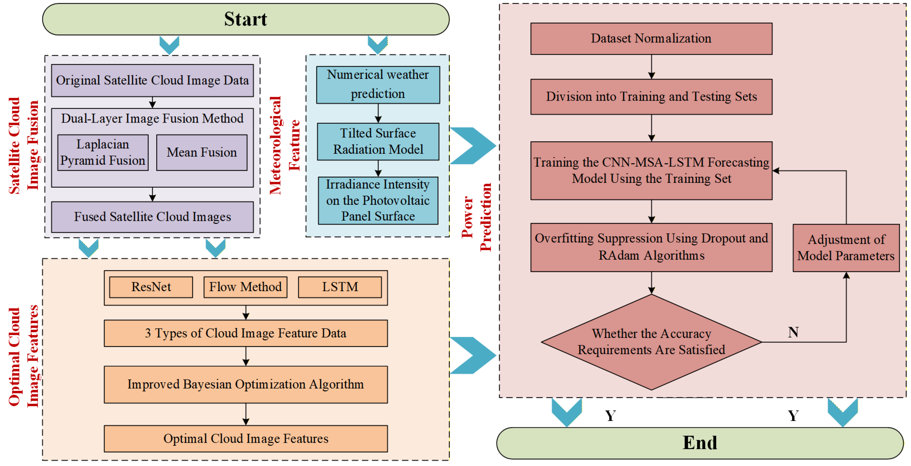
The flowchart of the IBO-CNN-MSA-LSTM PV power prediction model is illustrated in Figure 8. The steps are as follows:

Figure 8. Flowchart of PV power prediction based on the IBO-CNN-MSA-LSTM model.

Step 1: The original satellite cloud images are preprocessed. According to the characteristics of different spectral bands, Laplacian pyramid fusion and mean fusion methods are applied to perform multispectral channel fusion, thereby enriching the satellite cloud image information and constructing a fused satellite cloud image dataset.

Step 2: Numerical Weather Prediction (NWP) meteorological data are selected, and a tilted surface radiation model is employed to obtain the irradiance intensity on the PV module surface. Correlation analysis of the meteorological features is then conducted.

Step 3: Historical cloud image feature data are used for prediction based on a residual network. Meanwhile, predicted cloud images are obtained using the optical flow method and the LSTM network, respectively. The Gray-Level Co-occurrence Matrix (GLCM) and discrete wavelet transform (DWT) are then applied to extract the corresponding predicted cloud image features, and highly correlated features are selected.

Step 4: Based on the predicted cloud image features obtained from the above three methods, the improved IBO algorithm is employed to perform multidimensional feature fusion, thereby obtaining fused predicted cloud image features with a high degree of matching to PV power.

Step 5: The fused predicted cloud image features are combined with meteorological features to construct a dataset. After normalization, the dataset is divided into a training set and a testing set, and the data are input into the CNN-MSA-LSTM PV power prediction model. A multi-head self-attention (MSA) mechanism is introduced to perform weighted modeling of the feature sequences output by the CNN. The feature sequences optimized by the MSA are then input into the LSTM network, where the gating structure is employed to capture both long-term and short-term temporal dependencies in the time series, thereby obtaining accurate and stable prediction results.

Step 6: Dropout and the RAdam optimization algorithm are employed to suppress overfitting. In addition, the predicted values are compared with the actual values to determine whether the prediction accuracy meets the required criteria. If the criteria are satisfied, the predicted values are output; otherwise, the relevant model parameters are adjusted and the prediction procedure is repeated.

Step 7: Prediction performance is assessed using error indicators, including mean absolute error (MAE) and root mean square error (RMSE). Meanwhile, different models are compared and evaluated based on these metrics.

5. Example Analysis

5.1. Data Source

In this paper, the data used come from a PV power station located in Baoding, Hebei Province, China (115.06° E, 38.73° N), and include historical time-series data of PV power generation, NWP data, and PV module information. The collected dataset includes 100 days of data from September 2018 to May 2019 [33]. The dataset is organized on a daily basis, with approximately ten days of data selected from each month. Since PV power output is zero at night, only data from 9:00 to 18:00 are selected. Based on the cloud motion speed and the prediction horizon, the coverage area of the satellite cloud images is defined as a circular region with a radius of approximately 100 km centered on the PV power station. Himawari-8 full-disk satellite cloud image data with a temporal resolution of 10 min are selected. The temporal resolution of the NWP data is 15 min, and linear interpolation is applied to align all data to a unified temporal resolution of 15 min. In addition, a tilted surface radiation model is employed to calculate the tilted irradiance and correct the solar radiation input [34,35]. The dataset is partitioned into training and test subsets, where the initial 80 days are allocated to model training and the final 20 days are reserved for performance evaluation. PV power prediction with a lead time of 2 h is conducted.

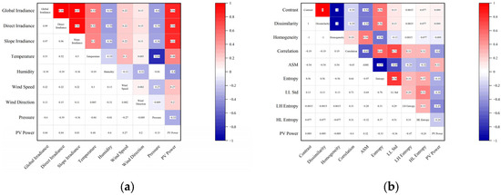
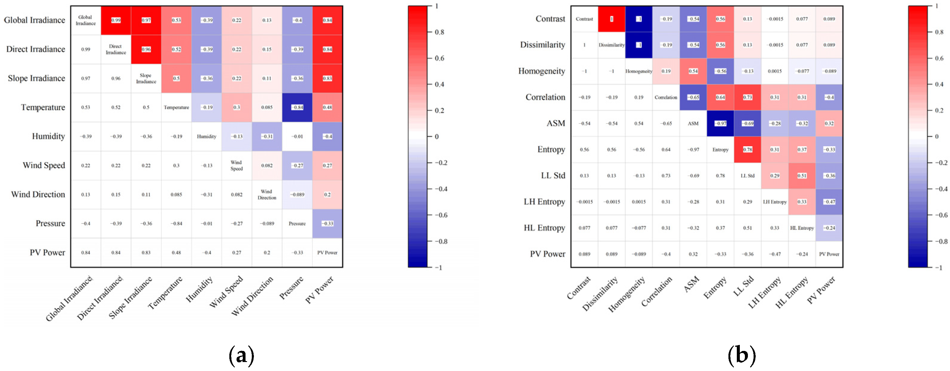
Considering the significant differences in how various meteorological variables influence PV power generation, Pearson correlation analysis is adopted to identify the NWP meteorological features. Meanwhile, correlation analysis is performed on the cloud image features derived from the Gray-Level Co-occurrence Matrix (GLCM) together with the wavelet transform. The results are shown in Figure 9.

Figure 9. (a) Meteorological feature correlation heat map. (b) Cloud image feature correlation heat map.

A greater absolute Pearson correlation coefficient corresponds to a stronger linear association. Correlation coefficients falling within [0.8, 1.0] are regarded as extremely strong correlations, [0.6, 0.8) as strong correlations, [0.4, 0.6) as moderate, [0.2, 0.4) as weak correlations, and [0, 0.2) as indicating the absence of correlation. As shown in Figure 9, the highly correlated features selected in this study are as follows: global horizontal irradiance, diffuse horizontal irradiance, tilted irradiance intensity, pressure, temperature, humidity, correlation, ASM, entropy, the standard deviation of the low-frequency component, and the entropy of the horizontal high-frequency component.

5.2. Analysis of Multiband Satellite Cloud Image Fusion

To verify the proposed image fusion method, image fusion quality is assessed using the peak signal-to-noise ratio (PSNR) and the structural similarity index measure (SSIM). The corresponding formulations are given as follows:

$$\{\begin{array}{c}\mathrm{P}\mathrm{S}\mathrm{N}\mathrm{R}=10{\mathrm{l}\mathrm{o}\mathrm{g}}_{10}({\displaystyle \frac{{\mathrm{M}\mathrm{A}\mathrm{X}}^2}{\mathrm{M}\mathrm{S}\mathrm{E}}})\\ \mathrm{S}\mathrm{S}\mathrm{I}\mathrm{M}={\displaystyle \frac{(2{\mathsf{\mu }}_{\mathrm{x}}{\mathsf{\mu }}_{\mathrm{y}}+{\mathrm{c}}_1)(2{\mathsf{\sigma }}_{\mathrm{x}\mathrm{y}}+{\mathrm{c}}_2)}{({\mathsf{\mu }}_{\mathrm{x}}^2+{\mathsf{\mu }}_{\mathrm{y}}^2+{\mathrm{c}}_1)({\mathsf{\sigma }}_{\mathrm{x}}^2+{\mathsf{\sigma }}_{\mathrm{y}}^2+{\mathrm{c}}_2)}}\end{array}$$

(20)

Here, MAX represents the maximum pixel value of the image; ${\mathsf{\mu }}_{\mathrm{x}}$ and ${\mathsf{\mu }}_{\mathrm{y}}$ are the mean values of x and y, respectively; ${\mathsf{\sigma }}_{\mathrm{x}}^2$ and ${\mathsf{\sigma }}_{\mathrm{y}}^2$ denote the variances of x and y; ${\mathsf{\sigma }}_{\mathrm{x}\mathrm{y}}$ represents the covariance of x and y; ${\mathrm{c}}_1={\left({\mathrm{k}}_1\mathrm{L}\right)}^2$ and ${\mathrm{c}}_2={\left({\mathrm{k}}_2\mathrm{L}\right)}^2$ are constants introduced for numerical stability; and L denotes the dynamic range of the pixel values.

The PSNR and SSIM values obtained using different fusion methods are presented in Table 1.

Table 1. PSNR and SSIM values of different fusion methods.

Fusion Scheme	PSNR	SSIM
Laplacian Pyramid Fusion + Guided Filtering Fusion	17.98	0.7736
Guided Filtering Fusion + Mean Fusion	27.97	0.6640
Brovey Fusion + Laplacian Pyramid Fusion	28.01	0.3822
Laplacian Pyramid Fusion Only	28.15	0.5156
Mean Fusion Only	27.96	0.6555
Laplacian Pyramid Fusion + Mean Fusion (Proposed Method)	28.18	0.7997

Higher PSNR and SSIM values indicate better image fusion quality. As shown in Table 1, the PSNR and SSIM values obtained using the proposed method are significantly higher than those obtained using other methods. This indicates that the quality of the fused satellite cloud images produced by the proposed method is relatively high. Compared with the mean fusion method alone, the PSNR and SSIM values obtained using the proposed method increased by 0.79% and 22%, respectively. The results indicate that the satellite cloud images fused using the proposed method not only retain cloud information from different bands and wavelengths but also reduce the differences in brightness temperature data in the infrared band. This validates the effectiveness of the proposed satellite cloud image fusion method.

5.3. Predicted Cloud Images and Their Feature Analysis

In this study, RMSE and MAE are adopted to evaluate the prediction errors of cloud image features at different time scales for the ResNet model. The formulations of RMSE and MAE are given as follows:

$$\{\begin{array}{c}\mathrm{RMSE}={\displaystyle \frac{1}{\mathrm{N}}}{\displaystyle \sum _{\mathrm{i}=1}^{\mathrm{N}}}\sqrt{{\displaystyle \frac{1}{\mathrm{n}}}{\displaystyle \sum _{\mathrm{i}=1}^{\mathrm{n}}}{({\mathrm{F}}_{\mathrm{i}}-{\widehat{\mathrm{F}}}_{\mathrm{i}})}^2}\\ \mathrm{MAE}={\displaystyle \frac{1}{\mathrm{N}}}{\displaystyle \sum _{\mathrm{i}=1}^{\mathrm{N}}}\left|{\mathrm{F}}_{\mathrm{i}}-{\widehat{\mathrm{F}}}_{\mathrm{i}}\right|\end{array}$$

(21)

Here, ${\mathrm{F}}_{\mathrm{i}}$, ${\widehat{\mathrm{F}}}_{\mathrm{i}}$, and $\overline{\mathrm{F}}$ denote the actual feature value, predicted feature value, and mean of the actual feature values, respectively, and N represents the number of predicted features.

NWP meteorological features and historical power generation data are used as the input features. After normalization, ResNet is applied to predict the extracted cloud image features at different future time scales. The prediction errors of the cloud image features at different time scales are presented in Table 2.

Table 2. Prediction errors of cloud image features at different time scales.

Feature	RMSE
	0.5 h	1 h	1.5 h	2 h
Correlation	0.0200	0.0178	0.0211	0.0206
ASM	0.0959	0.1110	0.1252	0.1095
Entropy	0.2336	0.2421	0.2692	0.3040
LL_std	0.4182	0.5424	0.4485	0.8185
LH_entropy	1.6586	1.8516	1.5324	1.6295
Feature	MAE
	0.5 h	1 h	1.5 h	2 h
Correlation	0.0164	0.0140	0.0162	0.0161
ASM	0.0746	0.0845	0.0936	0.0835
Entropy	0.1794	0.1808	0.2034	0.2340
LL_std	0.3016	0.3916	0.3481	0.5619
LH_entropy	1.2624	1.3217	1.1808	1.2008

Smaller RMSE and MAE values indicate lower prediction errors and better prediction performance. As shown in Table 2, the predicted cloud image features obtained using the ResNet method exhibit good accuracy at 0.5 h, 1.0 h, 1.5 h, and 2.0 h. Compared with the other features, the entropy of the horizontal high-frequency component shows relatively larger errors. At the 1 h time scale, its RMSE and MAE reach their maximum values of 1.8516 and 1.3217, respectively, but remain within an acceptable range.

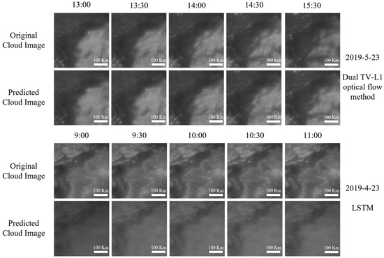
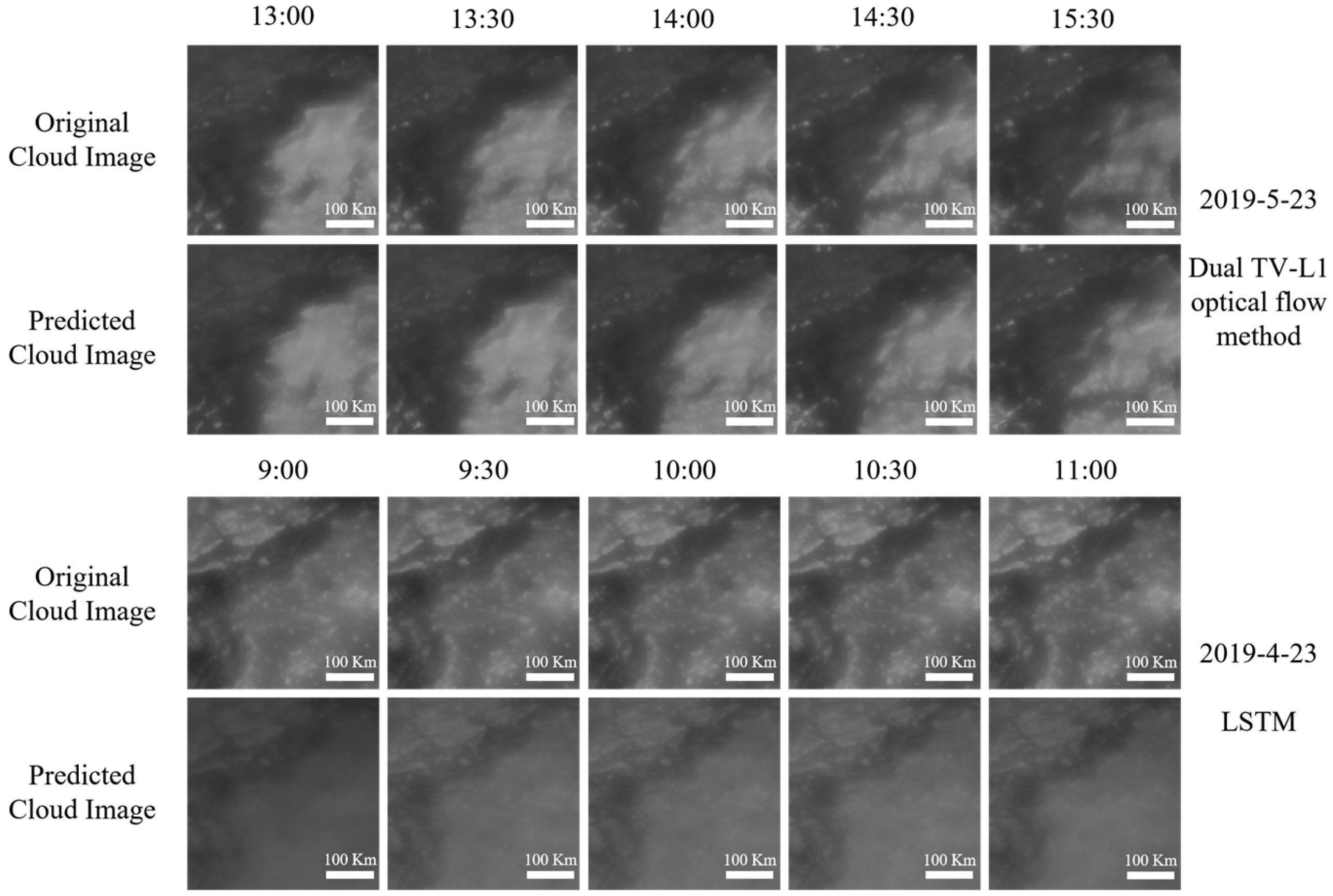
Using the Dual TV-L1 optical flow method and the LSTM network, satellite cloud images at different future time scales are predicted from historical cloud images. In this study, the predicted cloud images on 23 April 2019, and 23 May 2019 are selected for comparison. The comparison results are shown in Figure 10.

Figure 10. Comparison of predicted cloud images.

As shown in Figure 10, both the Dual TV-L1 optical flow method and the LSTM network can predict the basic motion trajectories and general texture contours of cloud layers, exhibiting good similarity to the original cloud images. The structural similarity index measure (SSIM) is used to verify the accuracy of the prediction results. The results are presented in Table 3.

Table 3. Prediction errors of cloud images at different time scales.

Feature	SSIM
	0.5 h	1 h	1.5 h	2 h
Dual TV-L1 Flow Method	0.8603	0.8106	0.7827	0.7660
LSTM	0.8382	0.8389	0.8367	0.8300

As shown in Table 3, the minimum and maximum SSIM values obtained with the Dual TV-L1 optical flow method and LSTM are 0.7660 and 0.8603, respectively. These results indicate that the predicted cloud images generated by both methods exhibit good similarity to the actual cloud images.

5.4. PV Power Prediction Results and Analysis

To make the role of the main modules in the proposed framework clearer, the following ablation and comparative analyses are organized around three aspects: the dual-stage cloud image fusion module, the multidimensional fusion module for predicted cloud features, and the complete IBO-CNN-MSA-LSTM forecasting framework.

5.4.1. Dataset Cross-Validation Analysis

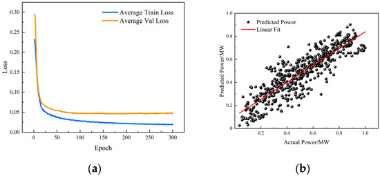
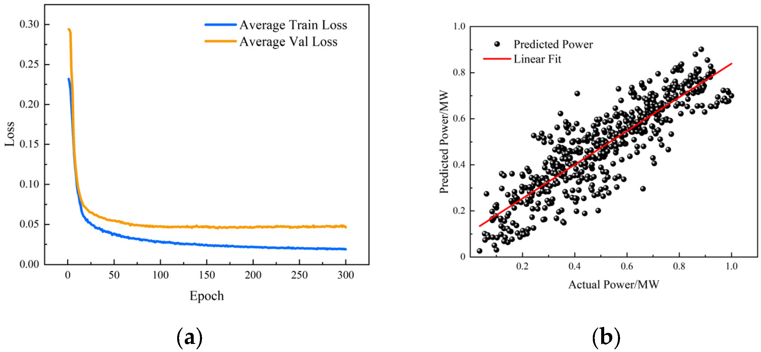
Dataset size plays an important role in determining both the accuracy and the generalization ability of a predictive model. In this study, only one dataset is available, and it contains 100 days of observations. Under this condition, the complexity of the model still leaves some possibility of overfitting, even though Dropout and the RAdam optimizer are introduced during training. Dropout helps prevent the network from depending too heavily on a small set of features by randomly deactivating neurons, but an overly aggressive setting may also weaken the learning process. RAdam, on the other hand, can improve optimization stability, yet its effect still depends on how the gradients and learning rate are controlled during training. For this reason, cross-validation is further introduced so that the model can be examined under different data partitions while preserving its generalization performance. Because the data are time-dependent, a time-series cross-validation strategy is adopted. The dataset is divided into five subsets, with each training set containing only earlier observations and each validation set representing later data. The corresponding validation results are presented in Figure 11.

Figure 11. (a) Average loss curve. (b) Scatter plot of predicted power and actual power.

As shown in Figure 11a, both the average training loss and the average validation loss decrease gradually before reaching a relatively stable level, which suggests that the model converges consistently across different data splits without obvious signs of overfitting. Figure 11b further shows a clear linear correspondence between the predicted and actual PV power values, indicating that the model retains good predictive ability. Taken together, these results suggest that the proposed model remains stable under different data partitions and exhibits a reasonable level of generalization.

5.4.2. Impact of Cloud Image Fusion on Power Prediction

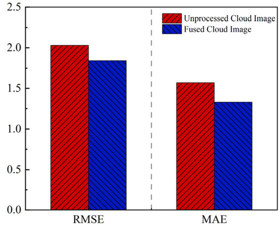
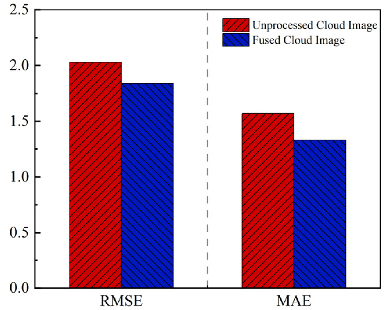
To validate the impact of the cloud image fusion module on power prediction, an ablation experiment was conducted by comparing the results with and without fused cloud images while keeping the other inputs unchanged. The comparison of prediction errors under the two conditions is shown in Figure 12. As shown in Figure 12, compared with the scheme using unfused cloud images, the RMSE and MAE of the scheme using fused cloud images are reduced by 9.36% and 15.29%, respectively. These results indicate that using fused cloud images can effectively reduce PV power prediction errors. This suggests that cloud image features can reflect cloud motion trajectories to a certain extent. The use of fused cloud images enriches the cloud information, thereby reducing PV power prediction errors and improving prediction accuracy.

Figure 12. Comparison of PV power prediction errors using unfused cloud images and fused cloud images.

5.4.3. Impact of Different Cloud Image Feature Inputs on Power Prediction

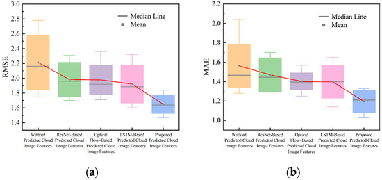
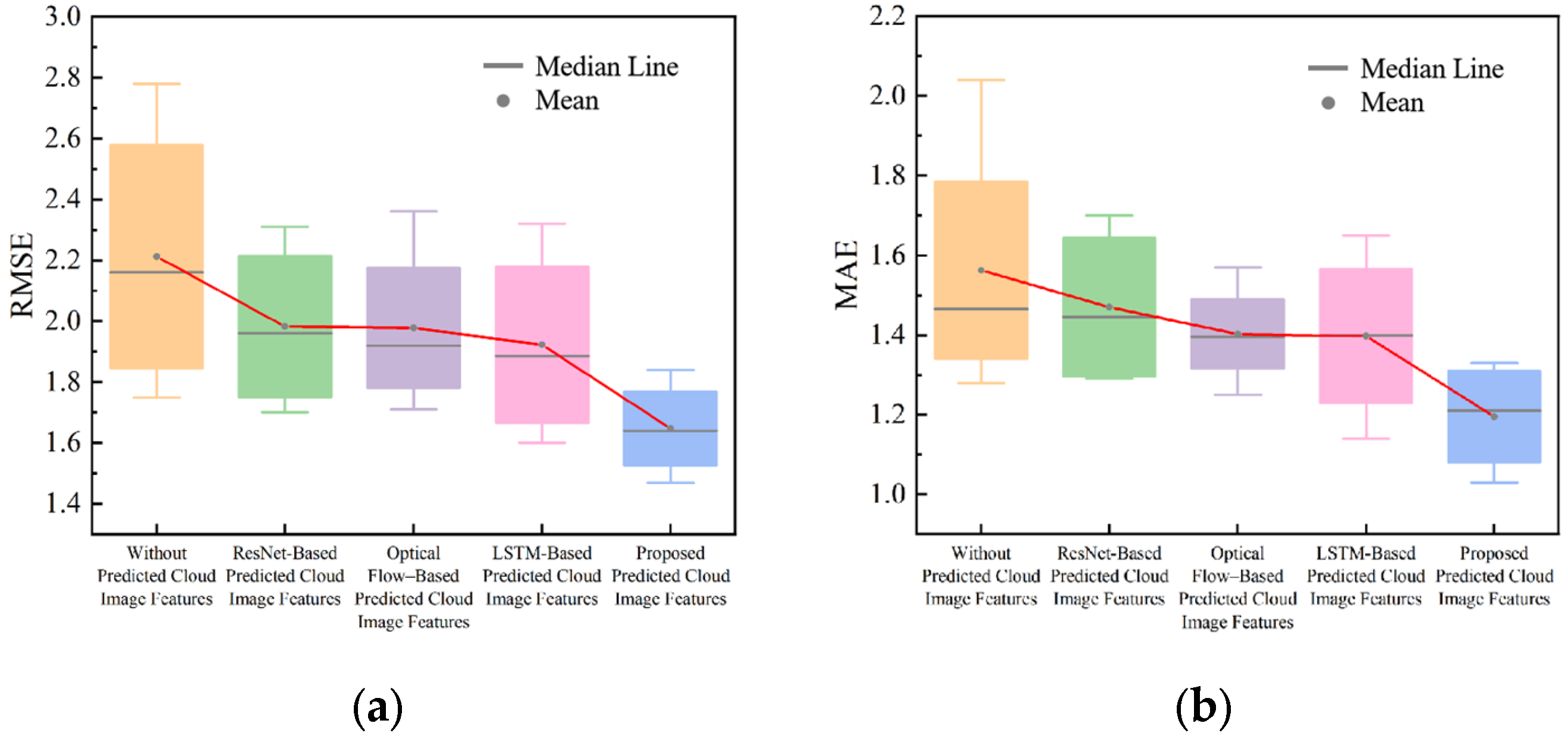
This section mainly examines the impact of multidimensional fused cloud image features on power prediction. RMSE and MAE are used as evaluation metrics, with time scales ranging from 0.5 h to 2.0 h. The power prediction results are compared among four schemes: predicted cloud image features obtained using ResNet, optical flow-based predicted cloud image features, LSTM-based predicted cloud image features, and the proposed multidimensional fused cloud image feature extraction method. The error box plots of the four schemes are shown in Figure 13, and the corresponding PV power prediction errors for the different cloud image feature extraction methods are listed in Table 4.

Figure 13. (a) PV power prediction RMSE box plot; (b) PV power prediction MAE box plot.

Table 4. PV power prediction errors using different cloud image feature extraction methods.

Cloud Image Feature Extraction Methods	RMSE
	0.5 h	1 h	1.5 h	2 h
Without Cloud Image Features	1.75	1.94	2.38	2.78
ResNet-Based Predicted Features	1.70	1.80	2.12	2.31
Optical Flow–Based Predicted Cloud Image Features	1.71	1.85	1.99	2.36
LSTM-Based Predicted Cloud Image Features	1.60	1.73	2.04	2.32
Predicted Cloud Image Features Obtained by the Proposed Method	1.47	1.58	1.70	1.84
Cloud Image Feature Extraction Methods	MAE
	0.5 h	1 h	1.5 h	2 h
Without Cloud Image Features	1.28	1.40	1.53	2.04
ResNet-Based Predicted Features	1.30	1.29	1.59	1.70
Optical Flow–Based Predicted Cloud Image Features	1.25	1.38	1.41	1.57
LSTM-Based Predicted Cloud Image Features	1.14	1.32	1.48	1.65
Predicted Cloud Image Features Obtained by the Proposed Method	1.03	1.13	1.29	1.33

As shown in Figure 13, the RMSE values for PV power prediction based on predicted cloud image features obtained using ResNet, optical flow, LSTM, and the proposed method are 2.31, 2.36, 2.32, and 1.84, respectively, with corresponding MAE values of 1.70, 1.57, 1.65, and 1.33. The PV power prediction results obtained using the proposed predicted cloud image features exhibit the best accuracy at different time scales, with the smallest error distribution and the lowest average errors. This is because the single cloud image features extracted by the ResNet, optical flow, and LSTM methods cannot provide comprehensive cloud and radiative information. In contrast, the proposed method fully considers variations in cloud-related factors, such as cloud thickness, temperature, and dynamic changes, which directly affect solar radiation absorption. The method analyzes multidimensional cloud image features, integrates different types of cloud features, and obtains fused features through weight matching, thereby enhancing sensitivity to key meteorological factors affecting PV power. The prediction model using the fused features can more comprehensively capture the complex effects of cloud layers on PV output, thereby improving the robustness of the prediction results. As shown in Table 4, the PV power prediction accuracy achieved using the proposed predicted cloud image features is the highest. Compared with the models based on ResNet, optical flow, and LSTM alone, the maximum reductions in RMSE and MAE reach 20.69% and 19.39%, respectively, demonstrating the feasibility and effectiveness of the proposed method.

5.4.4. Validation of Prediction Results Based on the IBO-CNN-MSA-LSTM

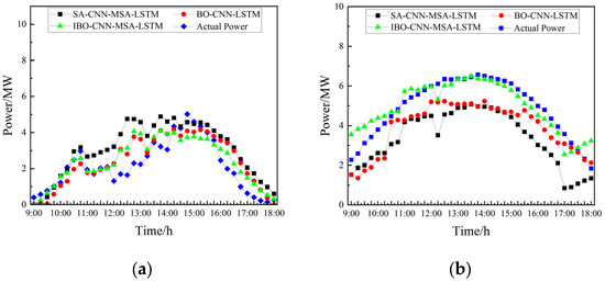
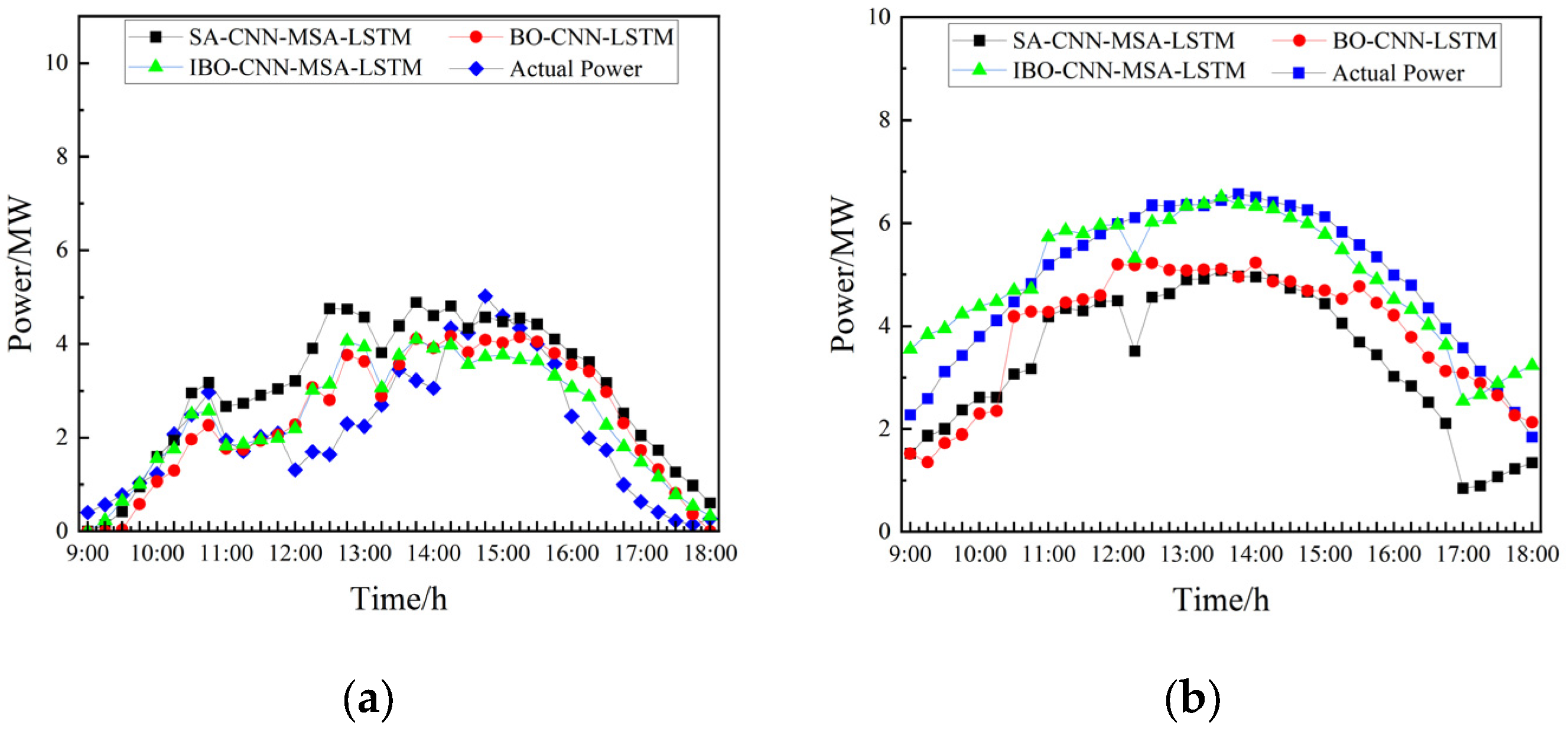
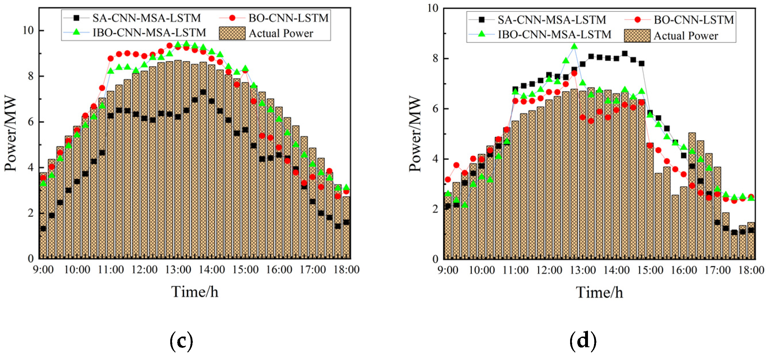
To validate the effectiveness of the proposed IBO-CNN-MSA-LSTM method, a 2 h ahead PV power prediction is conducted using datasets under different weather and seasonal conditions, and the proposed method is compared with the SA-CNN-MSA-LSTM and BO-CNN-LSTM models.

Given the time span of the dataset, it is divided into cold-season and warm-season subsets to verify the performance of the prediction model under different meteorological conditions. The specific results are shown in Figure 14 and Table 5. The proposed model demonstrates strong predictive capability under both seasonal conditions. In the warm season, due to more active cloud motion, the overall prediction error increases, but the proposed model still exhibits strong cross-season adaptability.

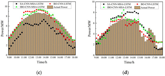
Figure 14. (a) PV power prediction results under cold-season; (b) PV power prediction results under warm-season; (c) PV power prediction results under clear-sky conditions; (d) PV power prediction results under fluctuating weather conditions.

Table 5. PV power prediction errors of different models under different weather conditions.

Weather Type	Error Metric	SA-CNN-MSA-LSTM	BO-CNN-LSTM	IBO-CNN-MSA-LSTM
Clear-Sky Conditions	RMSE	1.73	1.08	1.06
	MAE	1.46	0.82	0.76
Fluctuating Weather Conditions	RMSE	2.35	2.36	2.20
	MAE	1.73	1.78	1.70
SeasonalType	Error Metric	SA-CNN-MSA-LSTM	BO-CNN-LSTM	IBO-CNN-MSA-LSTM
Cold-Season	RMSE	2.05	1.73	1.61
	MAE	1.58	1.33	1.31
Warm-Season	RMSE	2.24	1.78	1.65
	MAE	1.84	1.45	1.33

For different weather scenarios, the prediction results and error metrics of each model are also analyzed. As shown in Figure 14c, under sunny weather, PV power output shows no significant fluctuations, and the prediction errors of the three methods are therefore similar. Compared with the BO-CNN-LSTM model, the prediction accuracy of the improved IBO-CNN-MSA-LSTM model is improved by 7.32%.

As shown in Figure 14d, under fluctuating weather conditions, rapid cloud motion leads to significant variations in PV power output, which greatly affect prediction accuracy. In this scenario, the IBO-CNN-MSA-LSTM model can capture richer feature information through the integration of cloud image features. Additionally, the incorporation of the MSA mechanism enhances the model’s global dependency modeling capability, enabling it to better track the evolution of cloud and meteorological features. Consequently, the RMSE of the IBO-CNN-MSA-LSTM model is reduced by 6.78% and 6.38% compared with the BO-CNN-LSTM and SA-CNN-MSA-LSTM models, respectively, while the MAE is reduced by 4.49% and 1.73%. Therefore, the proposed method shows better performance under fluctuating weather conditions.

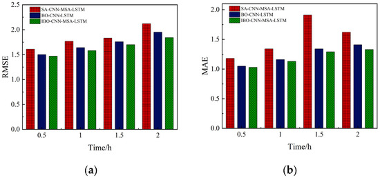
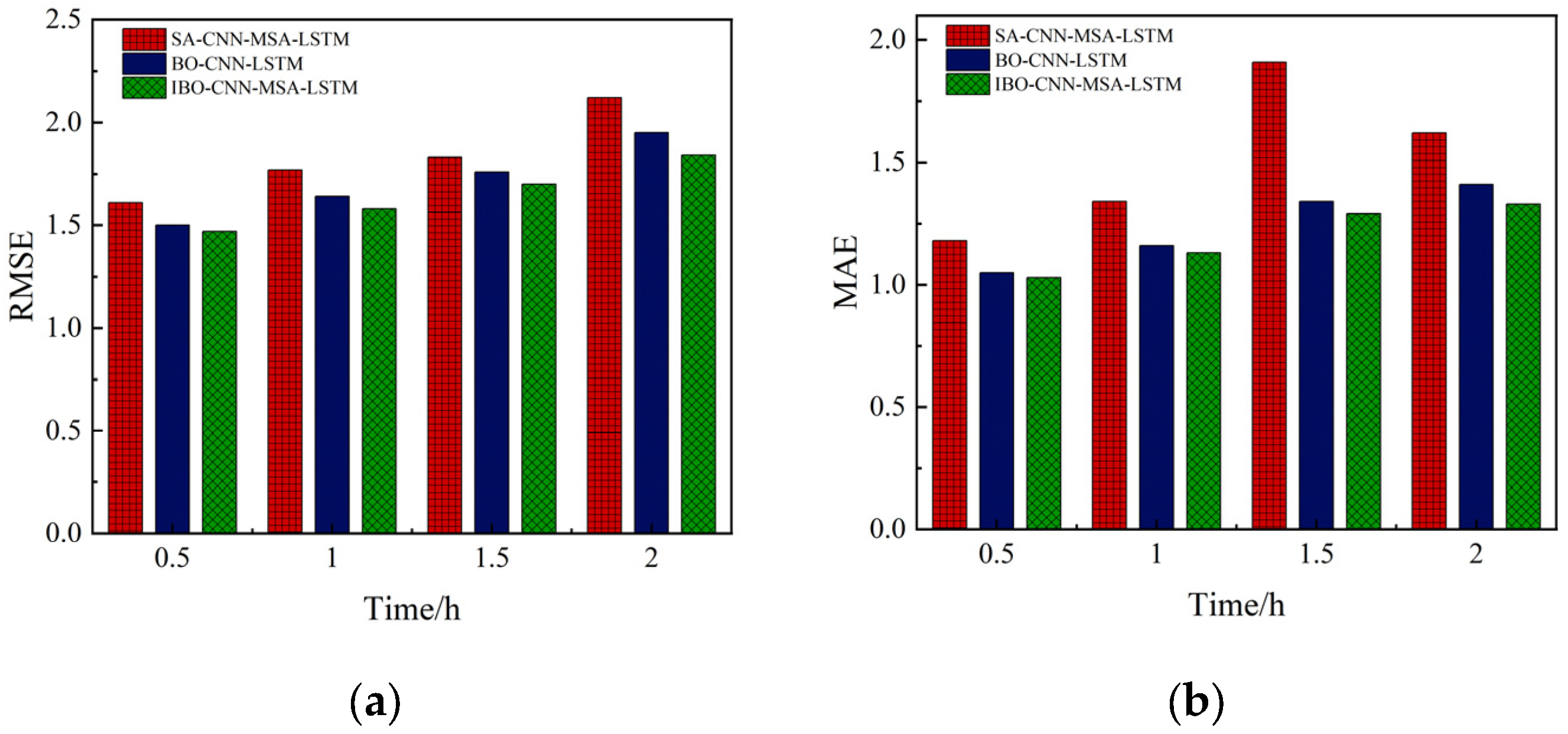
To further examine the performance of the proposed framework under different forecasting horizons, PV power prediction is conducted with lead times of 0.5 h, 1.0 h, 1.5 h, and 2.0 h using the three models mentioned above. The prediction error results are shown in Figure 15. As shown in Figure 15, the prediction errors gradually increase as the prediction time horizon increases. The proposed method consistently yields the lowest prediction errors and the highest accuracy across all prediction time horizons.

Figure 15. (a) PV power prediction RMSE at different time horizons; (b) PV power prediction MAE at different time horizons.

6. Conclusions

Cloud occlusion has a significant impact on electricity production in photovoltaic power plants, resulting in uncertainty and intermittency in PV output and posing challenges for optimal power system dispatch. To enhance photovoltaic power forecasting accuracy, this study concentrates on the multidimensional feature representation of satellite cloud images and an efficient prediction model. A prediction framework is constructed based on dual-layer image fusion, improved Bayesian optimization, and multi-head self-attention-based temporal modeling, forming a hierarchical modeling system of “feature enhancement–feature optimization–power prediction.” The main conclusions are as follows:

(1)

Based on the image characteristics of different wavelengths within the same band and across different bands of satellite cloud images, a fusion scheme combining Laplacian pyramid fusion and mean fusion is proposed. The PSNR and SSIM values increase by 0.79% and 22%, respectively, which improves the quality of the fused cloud images and significantly reduces the influence of brightness temperature differences in the infrared band. This method effectively enriches cloud image feature information.

(2)

An improved adaptive BO algorithm (IBO) is proposed. The IBO algorithm is used to fuse different cloud image features and obtain optimal fused cloud image features. Compared with the predicted cloud image features obtained using the ResNet, optical flow, and LSTM methods, the proposed method achieves a maximum reduction of 20.69% in RMSE and 19.39% in MAE.

(3)

An IBO-CNN-MSA-LSTM PV power prediction method is proposed. Compared with the SA-CNN-MSA-LSTM and BO-CNN-LSTM methods, the proposed method achieves improvements of 6.32% and 5.91%, respectively. In PV power prediction at different time scales, the average RMSE and MAE are reduced by 3.68% and 3.47%, respectively, thereby effectively improving prediction accuracy.

From the perspective of engineering application, introducing the MSA module does increase the computational burden to some extent. Even so, its parallel processing property helps the model retain good operating efficiency, which makes it capable of satisfying the real-time or near-real-time requirements of short-term PV dispatch. Another practical advantage lies in the modular structure of the framework. By adjusting the input dimensions and the length of the time window, the model can be extended with relative flexibility to scenarios involving multiple weather stations, multiple PV plants, or even regional PV clusters. In other words, the proposed method improves forecasting accuracy without sacrificing computational efficiency or scalability, which supports its potential use in grid optimization and dispatch under high renewable energy penetration.

References

- Wang, L. Study on the Impacts of Large-Scale Photovoltaic Power Generation on Power Systems. Lamps Light 2024, 102–104. [Google Scholar]
- Liu, Z.; Wang, S. To Pool Strong Efforts to Advance the Global Energy Transition. State Grid News, 23 May 2025; p. 001.
- Dong, C.; Wang, Z.; Bai, J.; Jiang, J.; Wang, B.; Liu, G. Review of Ultra-short-term Forecasting Methods for Photovoltaic Power Generation. High Volt. Eng. 2023, 49, 2938–2951. [Google Scholar] [CrossRef]
- Jia, L.; Yun, S.; Zhao, Z.; Li, H.; Wang, S.; Yang, L. Recent Progress of Short-term Forecasting of Photovoltaic Generation Based on Artificial Neural Networks. Acta Energiae Solaris Sin. 2022, 43, 88–97. [Google Scholar] [CrossRef]
- Luo, J.; Wang, Y.; Su, D. Research Progress on Ground-Based Cloud Image Detection and Photovoltaic Power Forecasting. Electron. Compon. Inf. Technol. 2024, 8, 98–100. [Google Scholar]
- Deng, F.; Liu, T.; Wang, J.; Gao, B.; Wei, B.; Li, Z. Research on Photovoltaic Power Prediction Based on Multimodal Fusion of Ground Cloud Map and Meteorological Factors. Proc. Chin. Soc. Electr. Eng. 2025, 45, 7193–7206. [Google Scholar] [CrossRef]
- Gao, H.; Liu, M. Short-term Solar Irradiance Prediction from Sky Images with a Clear Sky Model. In Proceedings of the 2022 IEEE/CVF Winter Conference on Applications of Computer Vision (WACV), Waikoloa, HI, USA, 3–8 January 2022; pp. 3074–3082. [Google Scholar]
- Dissawa, L.H.; Agalgaonkar, A.P.; Robinson, D.; Godaliyadda, R.I.; Ekanayake, J.B.; Ekanayake, P.B.; Perera, S. On-Site Solar Power Forecasting Using Sky-Images. In Proceedings of the 2020 Australasian Universities Power Engineering Conference (AUPEC), Hobart, Australia, 29 November–2 December 2020; pp. 1–8. [Google Scholar]
- Yin, X.; Zhao, H.; Sun, W.; Guo, X.; Jiang, S.; Liu, Y. Enhancement and Fusion Research of FY-4A Sea Area Cloud Images. Hydrogr. Surv. Charting 2020, 40, 30–34. [Google Scholar]
- Wang, Y.; Wang, Y.; Liu, Y.; Yang, D.; Xie, X. Ultra-short-term prediction of offshore photovoltaic power based on satellite remote sensing muli-spectral cloud image. Control Decis. 2025, 40, 1136–1144. [Google Scholar] [CrossRef]
- Zheng, K.; Wang, L.; Hao, Y.; Wang, B. Ultra-short-term Prediction of Photovoltaic Power Based on Dataset Distillation. Proc. Chin. Soc. Electr. Eng. 2024, 44, 5196–5208. [Google Scholar] [CrossRef]
- Zhang, Q.; Wang, L.; Hao, Y.; Wang, B.; Che, J.; Guo, H. Ultra-short-term Solar Irradiance Prediction of Distributed Photovoltaic Power Stations Based on Satellite Cloud Images and Clear Sky Model. High Volt. Eng. 2022, 48, 3271–3281. [Google Scholar] [CrossRef]
- Si, Z.; Yang, M.; YU, Y.; Ding, T. Ultra-short-term Photovoltaic Power Prediction Method Based on Satellite Image Feature Region Positioning. High Volt. Eng. 2021, 47, 1214–1223. [Google Scholar] [CrossRef]
- Zhang, J.; Teng, J.; Li, X.; Tan, Z. Short-term Prediction of Photovoltaic Power based on Meteorological Features and Improved Transformer. J. Eng. Therm. Energy Power 2024, 39, 146–154. [Google Scholar]
- Bessho, K.; Date, K.; Hayashi, M.; Ikeda, A.; Imai, T.; Inoue, H.; Kumagai, Y.; Miyakawa, T.; Murata, H.; Ohno, T. An introduction to Himawari-8/9—Japan’s new-generation geostationary meteorological satellites. J. Meteorol. Soc. Jpn. Ser. II 2016, 94, 151–183. [Google Scholar] [CrossRef] [Scilit]
- Bosch, J.L.; Zheng, Y.; Kleissl, J. Deriving cloud velocity from an array of solar radiation measurements. Sol. Energy 2013, 87, 196–203. [Google Scholar] [CrossRef] [Scilit]
- Wang, S.; Xu, C.; Shi, C.; Zhang, Y. Study on Cloud Classification Method of Satellite Cloud Images Based on CNN-LSTM. Comput. Sci. 2022, 49, 675–679+783. [Google Scholar]
- Li, M.; Fan, Z.; Zhu, Y. The Feature Fusion Depth Estimation Algorithm Based on Laplacian Pyramid. Electron. Meas. Technol. 2025, 48, 183–188. [Google Scholar] [CrossRef]
- Yin, H.; Xiao, J. Laplacian Pyramid Generative Adversarial Network for Infrared and Visible Image Fusion. IEEE Signal Process. Lett. 2022, 29, 1988–1992. [Google Scholar] [CrossRef] [Scilit]
- Zhao, S.; Wang, Z.; Chen, Z.; Hu, J.; Zhou, Z. GLCM Texture Features of On-load Tap Changer and Fault Diagnosis Method Based on Improved Random Forest Algorithm. High Volt. Eng. 2022, 48, 3593–3601. [Google Scholar] [CrossRef]
- Ma, L.; Kong, X.; Guo, L.; Liu, Y.; Liu, X. Photovoltaic Power Forecasting Based on Maximum Overlap Discrete Wavelet Transform and Deep Learning. Acta Energiae Solaris Sin. 2024, 45, 576–583. [Google Scholar] [CrossRef]
- Qian, Y.; Zhang, J.; Huang, Q. Infrared and Visible Image Fusion Based on Discrete Wavelet Transform. J. Shanxi Univ. (Nat. Sci. Ed.) 2025, 1–15. [Google Scholar]
- He, K.; Zhang, X.; Ren, S.; Sun, J. Deep Residual Learning for Image Recognition. In Proceedings of the 2016 IEEE Conference on Computer Vision and Pattern Recognition (CVPR), Las Vegas, NV, USA, 27–30 June 2016; pp. 770–778. [Google Scholar]
- An, J.; Liu, G.; Zhu, J. Application of Farneback Optical Flow Method in Nowcasting. Software 2018, 39, 18–25. [Google Scholar]
- Yang, Q.; Wang, Y.; Liu, L.; Zhang, X. Adaptive fractional-order multi-scale optimization TV-L1 optical flow algorithm. Fractal Fract. 2024, 8, 179. [Google Scholar] [CrossRef] [Scilit]
- Doshi, H.; Kiran, N.U. A variational optical flow model for accurate motion estimation from rotational image sequences. SN Comput. Sci. 2024, 5, 359. [Google Scholar] [CrossRef] [Scilit]
- Li, T.; Zhang, T.; Zhou, Q. Research on Photovoltaic Power Generation Prediction Based on LSTM-Informer. In Proceedings of the 2024 IEEE 2nd International Conference on Image Processing and Computer Applications (ICIPCA), Shenyang, China, 28–30 June 2024; pp. 1045–1049. [Google Scholar]
- Chen, L.; Zhang, T.; Ma, Y.; Li, Y.; Wang, C.; He, C.; Lv, Z.; Li, N. A Bayesian-attack-graph-based Security Assessment Method for Power Systems. Electronics 2024, 13, 2628. [Google Scholar] [CrossRef] [Scilit]
- Yu, G.; Lu, L.; Yang, S.; Wang, S.; Yang, X.; Cheng, R. An Improved Hybrid Neural Network Ultra-short-term Photovoltaic Power Forecasting Method Based on Cloud Image Feature Extraction. Proc. Chin. Soc. Electr. Eng. 2021, 41, 6989–7003. [Google Scholar] [CrossRef]
- Wang, K.; Du, H.; Jia, R.; Liu, H.; Liang, Y.; Wang, X. Short-term Interval Probability Prediction of Photovoltaic Power Based on Similar Daily Clustering and QR-CNN-BiLSTM Model. High Volt. Eng. 2022, 48, 4372–4388. [Google Scholar] [CrossRef]
- Li, W.; Li, X.; Fan, P.; Zhang, H. Regional Electricity Sales Forecasting Based on Multi-head Attention Mechanism and Long Short-term Memory Network. Power Demand Side Manag. 2025, 27, 67–73. [Google Scholar]
- Huang, Y.; Zhou, C.; Zuo, K. An Introduction to Himawari-89—Japan’s New-Generation Geostationary Meteorological Satellites. J. Highw. Transp. Res. Dev. 2023, 40, 185–191+199. [Google Scholar]
- Yao, T.; Wang, J.; Wu, H.; Zhang, P.; Li, S.; Wang, Y.; Chi, X.; Shi, M. A photovoltaic power output dataset: Multi-source photovoltaic power output dataset with Python toolkit. Sol. Energy 2021, 230, 122–130. [Google Scholar] [CrossRef] [Scilit]
- Li, Y.; Li, Z.; Wang, X.; Liu, K.; Wang, Y.; Zhao, W. Research on Optimum TILT Angle for PV Array Based on Combination Models of Calculating Solar Radiation on Inclined Surface. Acta Energiae Solaris Sin. 2022, 43, 127–136. [Google Scholar] [CrossRef]
- Wang, D.; Liu, J.; Huang, Y.; Shi, B.; Jin, M. Photovoltaic Power Prediction Method Combinating Solar Radiation Calculation and CNN-LSTM. Acta Energiae Solaris Sin. 2024, 45, 443–450. [Google Scholar] [CrossRef]
Disclaimer/Publisher’s Note: The statements, opinions and data contained in all publications are solely those of the individual author(s) and contributor(s) and not of MDPI and/or the editor(s). MDPI and/or the editor(s) disclaim responsibility for any injury to people or property resulting from any ideas, methods, instructions or products referred to in the content. |
© 2026 by the authors. Licensee MDPI, Basel, Switzerland. This article is an open access article distributed under the terms and conditions of the Creative Commons Attribution (CC BY) license.