


Abstract
In hazardous material transportation route planning, complex environments, stringent safety requirements, and sparse rewards often cause traditional reinforcement learning methods to converge slowly and yield unstable policies. To address these issues, this paper proposes TAR-RL (Trend-Aware and Attention-Augmented Reward Redistribution Reinforcement Learning), which integrates reward redistribution and adaptive exploration to improve the efficiency and robustness of path planning. Specifically, a dynamic ε-greedy strategy based on Q-value trends is introduced to adaptively adjust the exploration rate. Meanwhile, the RUDDER framework decomposes and redistributes delayed rewards to strengthen learning signals at critical decision points. Furthermore, a multi-head attention mechanism is incorporated to model long-term dependencies between states and actions, improving return prediction accuracy. An intrinsic reward mechanism encourages proactive exploration and autonomous learning. Experiments on two grid environments with different complexity levels demonstrate that TAR-RL achieves faster convergence, higher success rates, and more stable training dynamics than baseline methods. These results indicate that TAR-RL is well-suited for safety-aware path planning in high-risk routing scenarios.
1. Introduction
China’s industrial sector is currently undergoing rapid and profound transformations, placing increasing demands on logistics systems, where HAZMAT (hazardous materials) transportation warrants particular attention. Hazardous materials typically encompass flammable, explosive, corrosive, and toxic chemical substances, which pose significantly higher safety risks compared with the transportation of ordinary goods. Consequently, the transportation process must adhere strictly to relevant laws, regulations, and safety standards to mitigate potential hazards. To ensure safety, hazardous material transportation should avoid high-risk cells, such as densely populated regions, flammable and explosive zones, and high-temperature facilities. This necessitates the design of safe and reliable transportation routes that minimize potential risks while maximizing efficiency under strict safety constraints. The inherent complexity and high risk associated with hazardous material transportation make its route planning far more challenging than that of conventional cargo. Even minor accidents can lead to severe consequences, including large-scale environmental damage and public safety threats. Therefore, achieving an optimal balance between transportation safety and operational efficiency has become a critical and unresolved challenge in the domain of intelligent logistics planning.
Traditional path planning algorithms, including exact, heuristic, and metaheuristic approaches, have demonstrated effectiveness in specific and well-defined scenarios. However, their performance often deteriorates in dynamic environments, under complex constraints, and in situations requiring real-time decision-making. In the early stages of research, mathematical modeling and graph-theoretic techniques were predominantly employed to address path planning challenges. The A* algorithm, an enhanced variant of Dijkstra’s algorithm, integrates heuristic search strategies by combining the accumulated path cost with heuristic estimates to determine the optimal route. Sun et al. [1] refined the heuristic function of A*, yet the algorithm remains highly dependent on heuristic design, leading to limited efficiency and increased computational complexity.
The D* algorithm, a dynamic extension of A*, demonstrates stronger adaptability to changing environments by enabling rapid path updates when obstacles appear or environmental conditions vary. Zhang et al. [2] further improved D*, allowing it to efficiently replan paths in response to environmental changes; however, the resulting trajectories often exhibit excessive turns and insufficient smoothness. With advancements in computational power and algorithmic research, intelligent optimization techniques inspired by evolutionary computation and biological mechanisms have been introduced. For example, Kuo et al. [3] developed an enhanced MOPSO (multi-objective particle swarm optimization) algorithm to address supply chain disruptions in a two-stage vehicle routing problem under time-window constraints. Similarly, Dai et al. [4] proposed an innovative approach for solving the home healthcare location-routing problem by integrating an adaptive competition mechanism into the SA (simulated annealing) algorithm, significantly improving solution quality and computational efficiency.
In parallel with routing and classical planning, intelligent vehicle research has increasingly shifted toward data-driven perception–prediction pipelines integrated with optimal control and runtime safety enforcement, enabling online reactions to dynamic hazards. A representative example is REACT, a runtime-enabled active collision-avoidance technique for autonomous driving that emphasizes safety under uncertain interactions [5]. These developments motivate a layered view of safety: our work addresses route-level HAZMAT planning on a risk-annotated grid, which can complement vehicle-level collision-avoidance/control modules in an integrated intelligent logistics stack.
In recent years, the rapid development of deep learning and reinforcement learning has propelled path planning into a more intelligent paradigm, enabling adaptive decision-making in complex and uncertain environments. For hazardous HAZMAT transportation, reinforcement learning-based methods such as DQN (Q-learning and Deep Q-Networks) have demonstrated strong applicability, as they can leverage historical trajectory data to autonomously adjust transportation routes and avoid high-risk cells. However, traditional Q-learning suffers from limited generalization capability, making it difficult to perform well in unfamiliar environments. As a result, it often exhibits slow convergence, prolonged learning times, and susceptibility to local optima.
To address these limitations, Li et al. [6] proposed an improved Q-learning algorithm that integrates an ε-greedy exploration strategy with Boltzmann exploration while incorporating heuristic search to narrow the search space and constrain the variation of directional angles. Fang et al. [7] proposed a path planning method that integrates an improved ACO (Ant Colony Optimization) algorithm with an enhanced Q-learning algorithm (IQL). This approach significantly enhances the search efficiency, path smoothness, and global optimization capabilities of SAR (Search and Rescue) robots operating in complex environments. Similarly, Li et al. [8] introduced a dynamic exploration factor into the Q-learning framework to balance exploration and exploitation in local path planning for UAVs (unmanned aerial vehicles). Furthermore, Hu et al. [9] proposed a method that integrates Fuzzy A*, quantum multi-stage Q-learning, and the APF (Artificial Potential Field) for mobile robot path planning. This approach employs Fuzzy A* to generate global paths, utilizes quantum multi-stage Q-learning to address local optimality issues, and incorporates APF for dynamic obstacle avoidance, thereby enhancing the efficiency and robustness of the path planning process.
This study proposes TAR-RL (Trend-Aware and Attention-Augmented Reward Redistribution Reinforcement Learning), an RL-based algorithm for efficient and safety-aware hazardous materials (HAZMAT) routing in grid environments with sparse/delayed rewards. Building upon the classical Q-learning framework, TAR-RL introduces a Q-trend-based adaptive ε-regulation mechanism to dynamically adjust exploration intensity, thereby accelerating convergence and improving learning stability. In addition, we employ a RUDDER-based reward redistribution framework to perform causal decomposition of delayed rewards, strengthening learning signals at critical decision states. Furthermore, a multi-head self-attention mechanism is integrated into the return prediction model to capture long-term dependencies in state–action sequences more effectively, improving return prediction accuracy and credit assignment. Finally, we design a risk-aware reward structure with external risk penalties and loop-avoidance to discourage unnecessary exposure to high-risk cells, while intrinsic shaping is used only to provide goal-directed guidance under sparse rewards. Practical hazardous materials logistics may further involve time-window constraints, fleet-level coordination, and continuous road networks. These extensions are beyond the scope of the current manuscript and are briefly discussed in Section Limitations and Future Work. In the 20 × 20 and 30 × 30 environments, TAR-RL improves the success rate from 72.11%/36.80% (Q-learning) to 80.34%/59.63%, respectively. These gains are accompanied by faster and more stable convergence trends in both step-count and reward curves. In our environment, entering a high-risk cell triggers a severe penalty () and immediate episode termination, which operationalizes “risk” as constraint violations during planning, so higher success rates together with higher average returns indicate improved safety and reduced risk exposure.
In summary, this study targets hazardous materials routing under sparse/delayed rewards and stringent safety requirements. To ensure the novelty is explicit and verifiable, the main contributions are listed below:
- (C1) We propose TAR-RL, a Q-learning enhancement with Q-trend adaptive ε-regulation to accelerate convergence and improve policy stability.
- (C2) We introduce a risk-aware reward design tailored to hazardous routing, combining external risk penalties (including terminal penalties for high-risk violations) and loop-avoidance to discourage exposure to high-risk cells, while goal-directed intrinsic shaping is used to support exploration under sparse rewards.
- (C3) We integrate RUDDER-based reward redistribution with an attention-enhanced return predictor to address delayed/sparse rewards and strengthen credit assignment at critical decision points.
- (C4) We provide a systematic empirical evaluation in obstacle/risk grid environments and report metrics for success, stability, and risk-related safety performance.
2. Theoretical Foundations
2.1. Reinforcement Learning
An RL [10] routing task is modeled as a Markov decision process (MDP) , where and denote the state and action spaces, is the transition probability, is the immediate reward, and is the discount factor. The optimal action-value function satisfies the Bellman optimality backup [11], as shown in Equation (1):
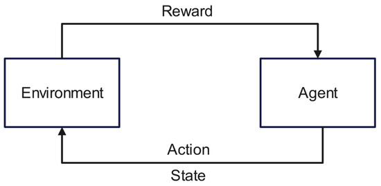
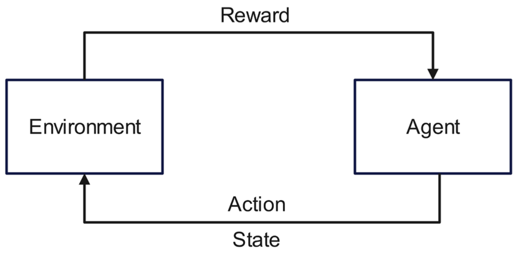
Figure 1 provides an overview of the agent–environment interaction in our grid-based routing setting.
Figure 1.
Reinforcement learning process diagram of the proposed grid-based routing setting with risk-aware terminal penalties.
2.2. Q-Learning Algorithm
Q-learning is an off-policy, model-free method that learns an approximation of from sampled transitions [12]. At each step, the action-value is updated by the temporal-difference rule as shown in Equation (2):
where is the learning rate. Action selection follows an -greedy policy [13] as shown in Equation (3): with probability choose , and with probability sample uniformly from .
where , is the exploration rate and is the size of the action space. If multiple actions maximize , the policy selects uniformly from the greedy set .
3. Design of the TAR-RL Algorithm
This paper proposes TAR-RL, an adaptive reinforcement learning algorithm that combines Q-value trend-based adjustment with RUDDER reward redistribution to self-adapt exploration via Q-trend-aware ε regulation and improve credit assignment, thereby endowing the agent with an “evolutionary capability,” i.e., a training-time self-improvement mechanism rather than an evolutionary optimizer such as a genetic algorithm. Designed specifically for HAZMAT transportation route optimization, the algorithm aims to maximize routing efficiency while ensuring transportation safety. Building upon the classical Q-learning framework, TAR-RL introduces four major improvements:
To address the limitations of the conventional ε-greedy strategy, in which the exploration rate ε cannot be dynamically adjusted in complex transportation scenarios, we propose a Q-value trend-based adaptive ε-regulation mechanism. This mechanism enables the agent to adjust the exploration rate dynamically according to variations in policy performance during the learning process. As a result, it improves policy optimization efficiency while avoiding excessive or insufficient stochastic exploration.
The algorithm incorporates a hierarchical reward structure that extends beyond the external rewards provided by the environment. An intrinsic reward mechanism is introduced to provide dense, goal-directed shaping under sparse external rewards, implemented as a scaled negative Euclidean distance to the goal. This intrinsic signal encourages purposeful exploration and supports the agent’s self-driven learning capability by guiding policy improvement during training. Risk avoidance is primarily enforced by the environment’s terminal penalties for entering high-risk cells. In addition, short cycles are discouraged via a repetition-avoidance penalty (reward = −10) without terminating the episode (done = False), which reduces dithering while keeping the episode bounded by the maximum step limit .
The algorithm integrates the RUDDER reward redistribution mechanism to perform causal attribution and decomposition of delayed returns, thereby strengthening feedback signals at critical decision points and improving both the specificity and stability of policy learning from the outset. Furthermore, a multi-head self-attention mechanism is incorporated into the return prediction model, enhancing the capability to capture long-term dependencies within state–action sequences. This not only improves risk identification and return prediction accuracy in complex environments but also provides a more principled and reliable basis for reward redistribution.
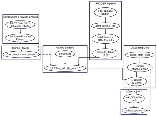
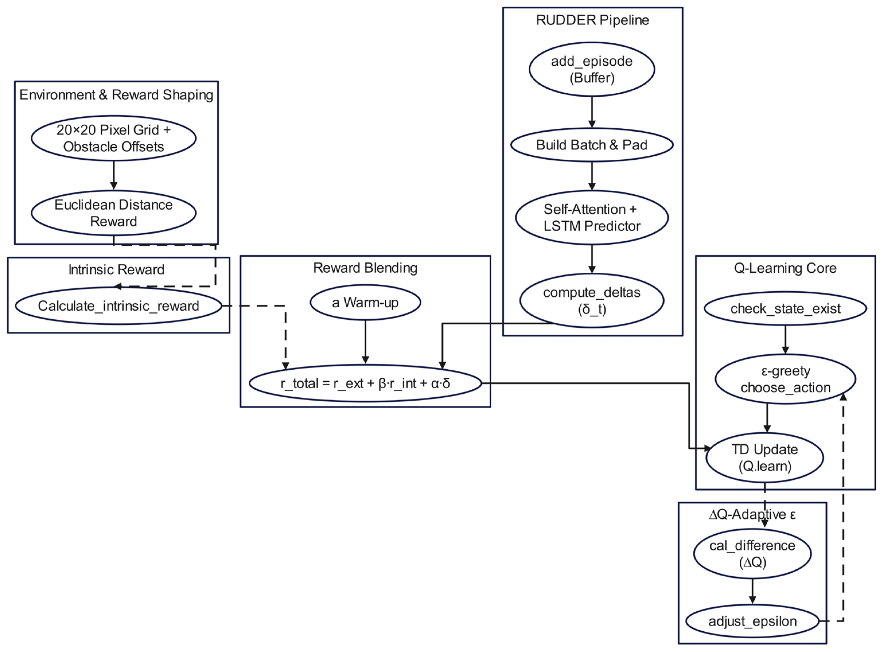
The overall architecture and execution workflow of the proposed TAR-RL algorithm, which is based on the dynamic ε-greedy strategy and the RUDDER reward redistribution mechanism, are illustrated in Figure 2.
Figure 2.
Overall Architecture and Workflow of the TAR-RL Algorithm. Arrows represent the flow of data between different components of the algorithm. The boxes represent key stages of the workflow, including the Environment & Reward Shaping, Intrinsic Reward Calculation, Reward Blending, RUDDER Pipeline, and Q-Learning Core. The diagram illustrates how data is passed through these modules, with key operations such as reward shaping, batch building, and action selection at each stage.
First, taking a simple obstacle environment as an example, the environment is represented by a 20 × 20 grid map, where obstacle location information is incorporated, and the Euclidean distance is used as the basis for computing the environmental reward signal. When executing actions in this environment, the agent not only relies on external environmental rewards but also computes intrinsic rewards to enhance the learning effectiveness.
As the core of reward redistribution, the RUDDER module first stores the state, action, and reward trajectories of each training episode into a buffer, from which training batches are constructed and sequences are padded. Leveraging a combination of the self-attention mechanism and an LSTM model, RUDDER then models these trajectories to compute the reward difference values δ at each time step. This process highlights the importance of delayed rewards, thereby refining the reinforcement signal and improving policy learning efficiency.
In the reward fusion stage, the algorithm combines the environmental reward (external reward), intrinsic reward, and the reward difference value computed by the RUDDER method through a weighted aggregation to form the total reward signal. The formulation is given as: . Here, α is gradually warmed up during the training process, thereby enabling a smooth incorporation of the RUDDER-based reward adjustment.
Subsequently, within the core Q-learning module, the agent selects actions at each step by consulting the current state in the Q-table and applying the ε-greedy strategy. After executing the action, the Q-value is updated using the TD (Temporal-Difference) method [14], progressively approximating the optimal policy. To further enhance learning efficiency, the algorithm introduces a ΔQ-based adaptive ε adjustment mechanism, which dynamically computes variations in Q-values and adjusts the exploration rate ε accordingly, thereby achieving a balance between exploration and exploitation in real time.
The overall workflow integrates environment design, reward redistribution, policy updating, and exploration-rate adjustment into a cohesive framework, thereby establishing an efficient and stable reinforcement learning-based path planning model. This integration significantly accelerates the agent’s learning process and enhances path planning performance in complex environments.
In summary, the proposed TAR-RL algorithm introduces multidimensional innovations across the policy learning layer, reward modeling layer, and task constraint layer. These advancements not only improve the adaptability and safety of reinforcement learning strategies but also provide a more practical and application-oriented solution to the constrained path optimization challenges inherent in hazardous materials transportation.
3.1. Dynamic Adaptive ε-Greedy Strategy
In the Q-learning method of reinforcement learning, ε is a critical hyperparameter in the ε-greedy strategy, playing a decisive role in balancing exploration and exploitation. However, in conventional approaches, ε is often set as a fixed value or predefined to follow exponential or linear decay. Such designs fail to reflect the agent’s actual learning progress during training, which may result in excessive exploration or premature convergence to suboptimal solutions.
To enhance policy flexibility and improve learning efficiency while maintaining a balance between exploration and exploitation, this paper proposes a dynamic adaptive ε-adjustment mechanism based on Q-value variations. By quantifying the magnitude of policy changes during each training episode, the mechanism adaptively adjusts the value of ε in real time, thereby achieving dynamic control over the exploration–exploitation trade-off. Specifically, the adjustment of ε is guided by the agent’s state–action feedback in the environment, and at the end of each training episode, ε is updated according to a defined variation measure derived from the learning process. Within a given episode, let the Q-tables before and after updates be denoted as and , respectively. The total Q-value variation (i.e., the difference measure) for that episode is then defined as shown in Equation (4):
The variation measure characterizes the overall degree of change in the current policy compared with the previous episode. A larger value of indicates that the policy is still undergoing rapid changes and remains in the exploration phase, whereas a smaller value of suggests that the policy is becoming stable, allowing for a gradual reduction of randomness. Based on this variation measure , ε is updated adaptively in an exponential manner. The adjustment rule is formulated as shown in Equation (5):
Here, and represent the upper and lower bounds of ε (e.g., 0 ≤ < ≤ 1), while k > 0 is an adjustment factor that controls the sensitivity of ε to the variation measure This updating rule ensures that ε fluctuates within the interval [, When the variation measure is large, the exponential term approaches zero, causing ε to remain close to , thereby encouraging the agent to continue exploration. Conversely, when the variation measure is small, ε tends toward , reinforcing exploitation of the acquired knowledge. In this way, the ε-greedy strategy adapts automatically according to the progress of learning.
This mechanism performs the computation of the variation measure and the update of ε at the end of each training episode. By embedding adaptivity into the dynamic ε-greedy strategy, the agent is encouraged to increase exploration during unstable policy phases and to reduce exploration as the policy stabilizes. This not only enhances the stability and efficiency of the learning process but also makes the approach particularly well-suited for environments with large state spaces or sparse reward signals.
3.2. Design and Integration of the Intrinsic Reward Mechanism
Intrinsic rewards are designed to encourage the agent to explore novel or insufficiently visited states within the environment. In scenarios where external rewards are sparse, intrinsic rewards [15] provide additional feedback signals, thereby motivating the agent to more effectively explore the state space and progressively approach the target regions.
In this study, an intrinsic reward function based on the distance to the target is employed, where the distance between the current state and the goal serves as a guiding signal for the agent’s behavior. Let the current state be and the goal position be . The intrinsic reward is then defined as the negative Euclidean distance [16] between the current state and the goal, as formulated in Equation (6):
Here, is a scaling factor, which is set to in our experiments, to control the weight of the intrinsic reward within the overall reward structure and to ensure that this component does not overwhelm the external reward signal. The intrinsic reward primarily functions by providing larger negative feedback when the agent is far from the goal and smaller negative feedback as it approaches the target. This design motivates the agent to move proactively toward the goal region and enables continuous learning, even in phases where external rewards are sparse or absent.
Furthermore, to further enhance the agent’s exploration efficiency, the intrinsic reward is integrated with the external reward through weighted fusion, forming the final composite reward signal for Q-value updates, as expressed in Equation (7):
Here, denotes the weighting coefficient of the intrinsic reward. When (i.e., under sparse external rewards), the nonzero intrinsic reward can still drive Q-value updates, thereby alleviating training stagnation caused by reward sparsity and accelerating policy convergence.
This mechanism significantly alleviates the challenge faced by traditional Q-learning in obtaining effective feedback during the early stages of training. Even when the agent does not directly trigger terminal conditions (such as success or failure), it can still receive meaningful feedback based on its proximity to the target, thereby enabling more efficient path learning and policy convergence. This approach not only enhances the agent’s exploratory capability in sparse-reward environments but also improves learning stability and training efficiency.
To further validate the effectiveness of the intrinsic reward mechanism, the reward trends of each training episode were recorded and visualized. Under the setting without intrinsic rewards, the agent typically requires extensive random trials before it can occasionally trigger the external reward at the target state, resulting in a slow learning process and a prolonged convergence cycle. In contrast, with the incorporation of intrinsic rewards, the agent can receive finer-grained feedback through negative distance rewards obtained while moving closer to the goal, even without reaching the terminal state. This continuous incentive plays a significant role in guiding the learning process and accelerating convergence.
3.3. RUDDER-Based Reward Redistribution
To address the challenge of delayed rewards, this study incorporates the RUDDER module [17], which redistributes environmental returns by tracing them back and decomposing them into the state–action pairs that critically influence the final outcome. This process improves both training efficiency and policy stability. In the proposed model, the RUDDER module consists of two main components: the training of the return prediction model and the application of reward redistribution.
3.3.1. Architecture of the Return Prediction Network
In this study, the RUDDER model employs a hybrid architecture that combines Multi-Head Attention [18] with a Long Short-Term Memory (LSTM) network [19] to perform trajectory return prediction. Each state st and action at is first processed through embedding layers to obtain state embeddings and action embeddings , respectively. The embedding vectors at each time step are then concatenated and fed into both the multi-head attention layer and the recurrent network. The multi-head attention mechanism enables the model to capture information from different positions of the sequence in parallel; within this model, it specifically enhances feature extraction at critical time steps (e.g., environmental turning points). The attention-processed sequence is subsequently passed into the LSTM, whose hidden states capture the temporal dependencies across the entire trajectory. Finally, a linear regression head is appended to the output of the LSTM, mapping the hidden state at the last time step into the predicted return value G_hat, as formulated in Equation (8):
Here, (,) denote the learnable parameters of the regression layer. At this stage, represents the estimated future cumulative discounted return starting from the current time step t. The overall architecture of the RUDDER module includes the following components: state embedding layer, action embedding layer, multi-head attention mechanism, LSTM network, and regression prediction head. This structure is designed to enable the model to predict the final return by learning from key events within the sequence.
3.3.2. Design of the Reward Redistribution Strategy
During the training phase, the RUDDER module supervises the return function at the trajectory level, enabling the pre-allocation of delayed rewards. Training data is collected by the add_episode function, which aggregates trajectories on an episode-by-episode basis. Each trajectory represents one episode and includes state–action–reward triples (s0, a0, r0), (s1, a1, r1), …, (sT, aT, rT), where each triple records the state, action, and corresponding immediate reward. Let denote the true discounted return for the trajectory. During model training, a mini batch is randomly sampled from the stored episodes, and the RUDDER model generates predicted returns through forward propagation. A regression loss function is then constructed, as shown in Equation (9), using the mean squared error (MSE):
Here, represents the model parameters, and denotes the batch size. Using backpropagation and gradient descent to optimize the loss function , the model is trained to minimize the difference between the predicted returns and the true returns for the i-th trajectory. This process aims to make the predicted returns as close as possible to the true returns. After multiple iterations of training, the RUDDER model learns to identify and emphasize the critical steps in the sequence that contribute significantly to the final return.
After training is complete, reward decomposition can be performed on any recorded trajectory: the model generates a predicted return for the state–action sequence at each time step t of the trajectory. The RUDDER redistributed reward at step t is then defined as shown in Equation (10):
It is assumed that . In this way, the sum of the rewards over all time steps equals , and reflects the marginal contribution of step t to the total return. According to the principles of RUDDER, this method effectively “backpropagates” the delayed final return to the key events, ensuring that the expected future return approaches zero. This approach simplifies subsequent Q-value learning by directly linking rewards to critical actions.
3.3.3. Reward Fusion Mechanism and α Warm-Up
After integrating the external reward, intrinsic reward, and RUDDER redistributed reward, the agent uses the combined reward signal for learning. Specifically, after receiving the external reward , intrinsic reward , and RUDDER redistributed reward at step t, the total reward can be defined as shown in Equation (11):
Here, is the weight of the intrinsic reward, and is the weight of the RUDDER reward. is introduced gradually using a “warm-up” strategy: during the early stages of training, to avoid instability in the model, is set to 0. As the number of training episodes increases and the RUDDER model becomes sufficiently reliable, starts to increase either linearly or exponentially. The linear warming-up strategy [20] for is defined as shown in Equation (12):
Specifically, before the training step , the RUDDER reward is not applied, i.e., the coefficient is set to 0 during the early training phase. After the training step , increases linearly until it reaches 1 at . In this way, as grows, the redistributed reward provided by RUDDER is gradually incorporated into the learning framework. When , the reward signal includes the complete redistributed reward ; conversely, when , the redistributed reward is completely ignored. Through the proposed reward fusion mechanism, the immediate reward used in each Q-learning update is the weighted reward . By tuning , the agent can first acquire basic policies during the initial phase of training and subsequently leverage the deeper return information revealed by the RUDDER model to further optimize the learning process.
The workflow of the TAR-RL algorithm is shown in Algorithm 1:
| Algorithm 1. TAR-RL algorithm |
| 1. Initialize the Q-table, ε, γ, η, β, α(t); initialize the RUDDER model and the buffer |
| 2. For each training episode: |
| 3. Reset the environment and initialize the state s0 |
| 4. While the episode is not finished: |
| 5. Select action at using the ε-greedy strategy; execute action at and observe the next state st+1 and external reward |
| 6. Calculate the intrinsic reward ←calculate_intrinsic_reward() |
| 7. Compute the initial combined reward |
| 8. Update the Q-value Q(st, at) ← Q-learning update rule. |
| 9. Store the tuple (st, at, , ) in the buffer |
| 10. Transition to the next state st ← st+1 |
| 11. Compute α ← get_alpha(episode), predict δt ← Ĝt − Ĝt+1 |
| 12. Compute the blended reward r_blend ← (1 − α)·rt + α·δt, and update the Q-value |
| 13. Store the transition; if the conditions for RUDDER model training are met, train the RUDDER model |
| 14. Adjust ε based on D (the Q-value difference), adjust_epsilon(D) |
| 15. End |
| 16.End |
4. Experimental Results and Analysis
4.1. Experimental Setup and Metrics
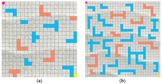
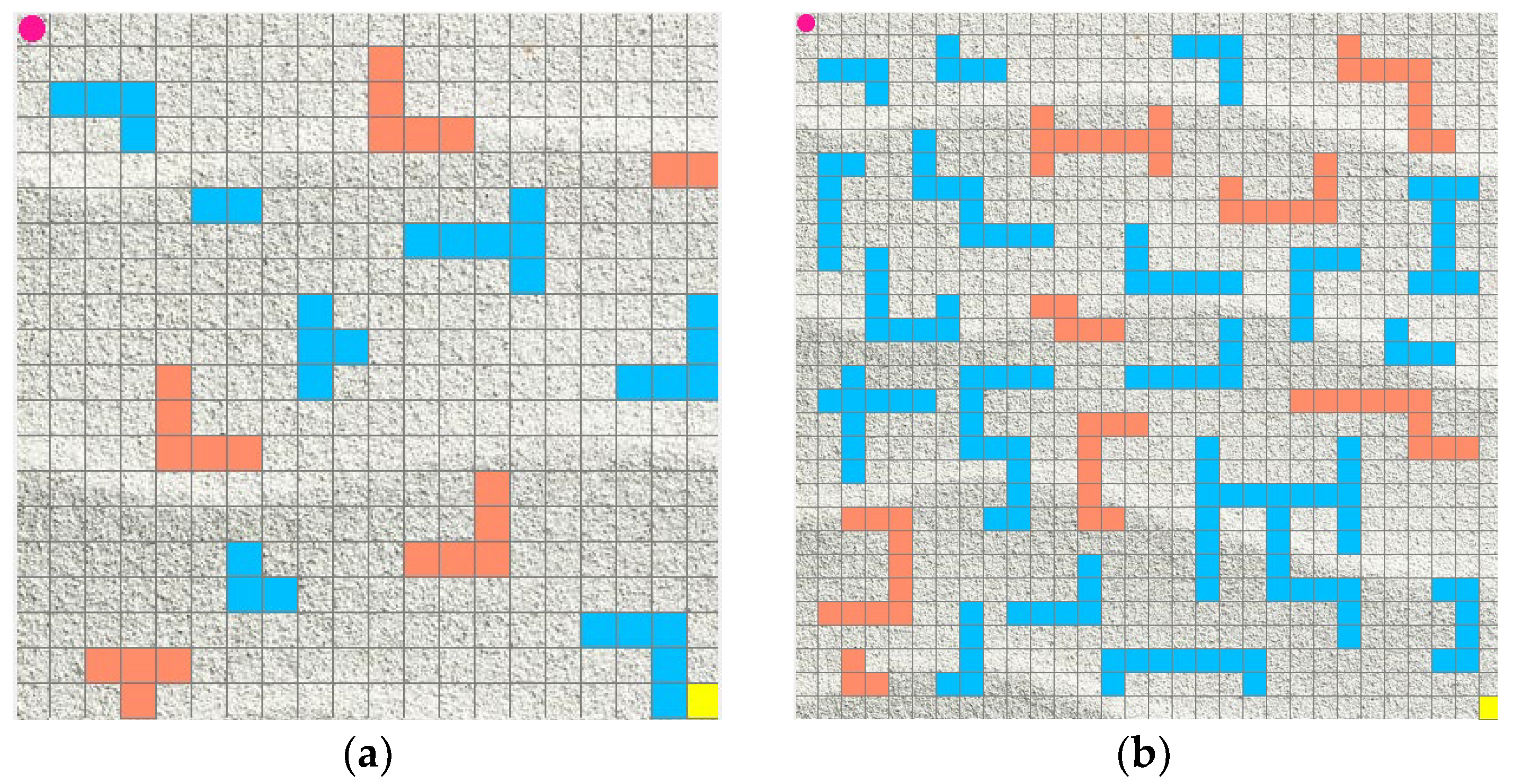
To validate the feasibility of the proposed algorithm in different environments, we simulate two grid maps, a simple 20 × 20 map and a complex 30 × 30 map, as shown in Figure 3.
Figure 3.
Simulated Grid Map. Blue cells indicate ordinary obstacles and orange cells indicate high-risk regions; the start and goal are marked in deep-pink and yellow, respectively. (a) Simple obstacle map; (b) complex obstacle map.
The deep-pink dot denotes the agent, whose initial position corresponds to the start cell. Blue cells form irregular regions of ordinary obstacle cells; stepping into any blue cell is treated as a collision that terminates the episode with a penalty of −50 (done = True). Orange cells form high-risk regions for hazardous-material transportation; entering any orange cell is treated as a safety violation that terminates the episode with a penalty of −100 (done = True). Blank cells are traversable free space, and the yellow cell indicates the goal. In both environments, ordinary obstacle and high-risk cells are deterministically placed by hard-coding pre-defined cell coordinates in the environment construction code: the 20 × 20 map contains 50 terminal non-traversable cells (29 ordinary obstacle cells and 21 high-risk cells), while the 30 × 30 map contains 207 terminal non-traversable cells (144 ordinary obstacle cells and 63 high-risk cells). The layouts are fixed across all methods and episodes for fair comparison.
Episode termination and loop handling: An episode ends if (i) the agent reaches the goal, (ii) it enters an ordinary obstacle cell (reward = −50, done = True) or a high-risk cell (reward = −100, done = True), or (iii) the number of steps exceeds the maximum limit . Looping is not used as an early-termination criterion; instead, short cycles are discouraged via a repetition-avoidance penalty (reward = −10, done = False), while bounds the episode length.
Evaluation protocol: We evaluate each method in two grid-based routing environments (20 × 20 and 30 × 30). For each method and each environment, we run 15,000 episodes, with a maximum of 150 steps per episode. The random seed is fixed to 42 for reproducibility. An episode terminates when the agent reaches the goal, enters an ordinary obstacle cell or a high-risk cell, or when the step limit (150 steps) is reached; the step-limit termination is treated as a failure to reach the goal.
Software and implementation details: All simulations and training were implemented in Python (version 3.9.18; Python Software Foundation, Wilmington, DE, USA). The return prediction network in the RUDDER module was implemented using PyTorch (version 2.0.1; PyTorch Foundation, part of The Linux Foundation, San Francisco, CA, USA). Numerical computations were performed with NumPy (version 1.26.4; NumFOCUS, Austin, TX, USA).
Success and Success Rate: An episode is considered successful if the agent reaches the goal state within 150 steps without terminating due to an ordinary obstacle or a high-risk cell. Let denote whether episode is successful. The Success Rate over episodes is computed as shown in Equation (13):
Here, is the total number of episodes, and if the final terminal state of episode is the goal; otherwise .
Average Reward: Let denote the episodic return (total reward) of episode , computed as the sum of step-wise rewards returned by the environment, i.e., , where is the number of executed steps in episode . The Average Reward over episodes is computed as shown in Equation (14):
In our implementation, denotes the total reward used for learning (including the extrinsic terminal penalties/rewards and the intrinsic distance-based term), and is computed as the mean episodic return over all 15,000 episodes.
Risk Violation Indicator: It is defined to capture whether an episode terminates due to entering a high-risk cell under our environment setting as shown in Equation (15):
Here, is a binary indicator for high-risk termination events in a single episode.
Risk Cost (RC): It quantifies the episode-level risk penalty consistent with the environment design, where a high-risk violation triggers a −100-terminal penalty as shown in Equation (16):
Here, denotes the risk cost per episode, and the factor corresponds to the magnitude of the high-risk penalty (−100) used in the environment.
Risk Violation Rate (RVR): It is defined as the proportion of evaluation episodes that end due to high-risk violations as shown in Equation (17):
Here, denotes the total number of evaluation episodes, and is the risk violation indicator of the -th episode.
A method is considered safer if it achieves higher SR while lowering the risk violation rate (RVR) and reducing severe terminal penalties associated with high-risk cells.
The relevant parameters set for this study are presented in Table 1.
Table 1.
Main Algorithm Parameter Settings.
4.2. Results and Discussion
Due to the two different grid environments used in this study, the number of steps required by the agent increases in the more complex grid environment. Therefore, for each of these environments, corresponding discount factors and RUDDER reward weight warm-up episodes were set to evaluate the algorithm’s performance.
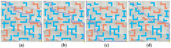
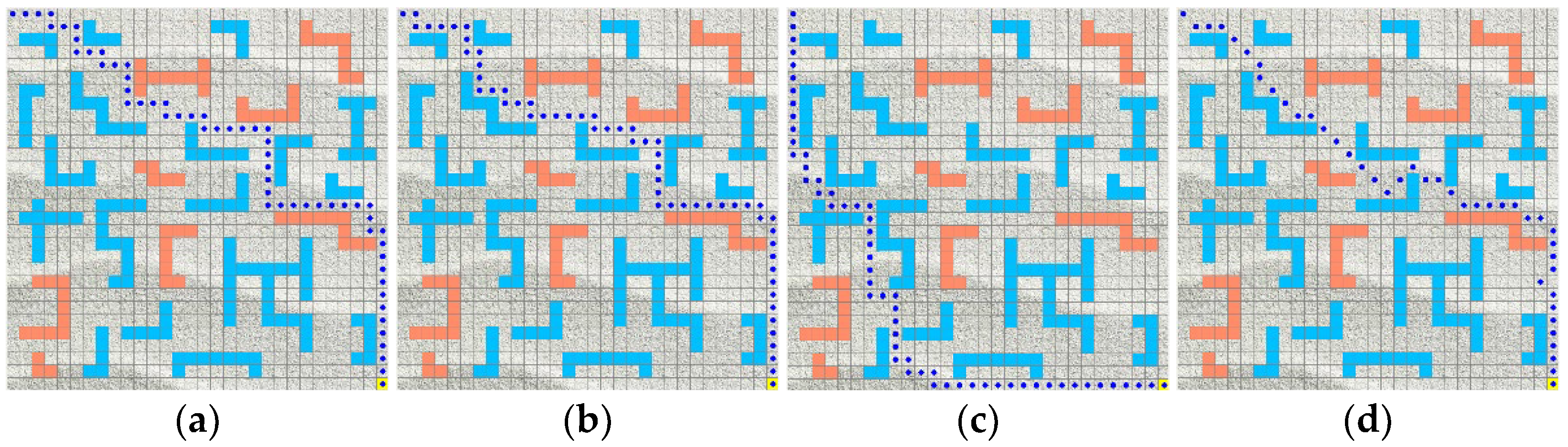
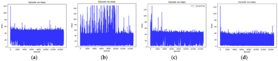
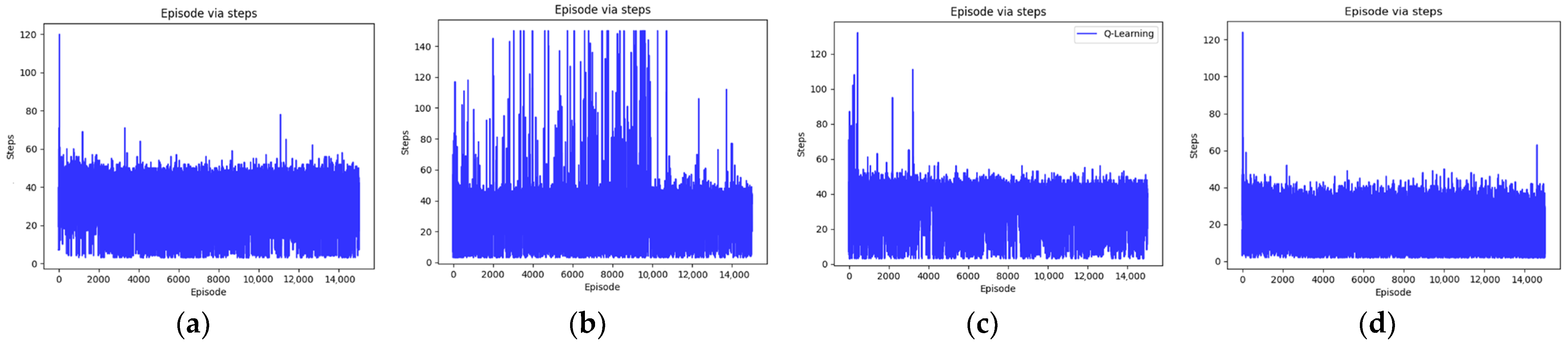
Based on the method proposed in this paper and using the parameter settings from Table 1, the path planning results obtained using the Q-learning algorithm and the proposed algorithm are shown in Figure 4 and Figure 5. The number of steps taken by the agent and the rewards obtained during the experiment are illustrated in Figure 6, Figure 7, Figure 8 and Figure 9. The experimental results for the DRQL (dynamic reward-enhanced Q-learning) algorithm [21] are also presented in Figure 4, Figure 5, Figure 6, Figure 7, Figure 8 and Figure 9.
Figure 4.
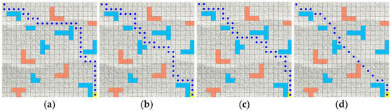
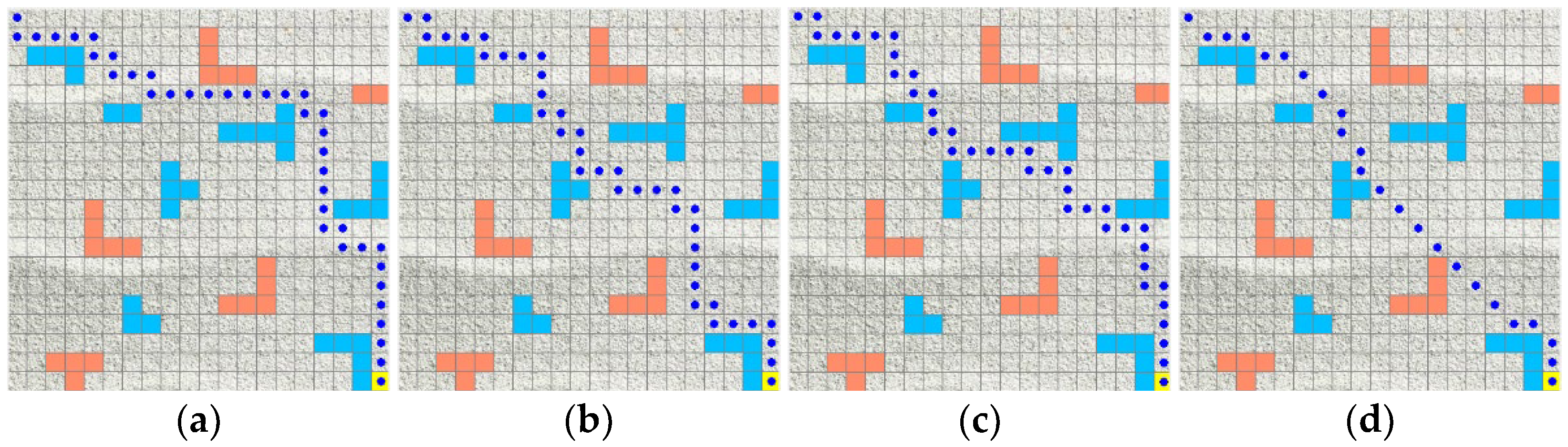
Comparison of Path Planning Results between the Q-learning Algorithm and the Proposed Algorithm in the Simple Obstacle Environment: (a) Q-learning; (b) AEG-QL; (c) TAR-RL; (d) DRQL. The blue dotted line indicates the planned path. Blue cells indicate ordinary obstacles and orange cells indicate high-risk regions, and the yellow cell indicates the goal.
Figure 5.
Comparison of Path Planning Results between the Q-learning Algorithm and the Proposed Algorithm in the Complex Obstacle Environment: (a) Q-learning; (b) AEG-QL; (c) TAR-RL; (d) DRQL. The blue dotted line indicates the planned path. Blue cells indicate ordinary obstacles and orange cells indicate high-risk regions, and the yellow cell indicates the goal.
Figure 6.
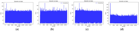
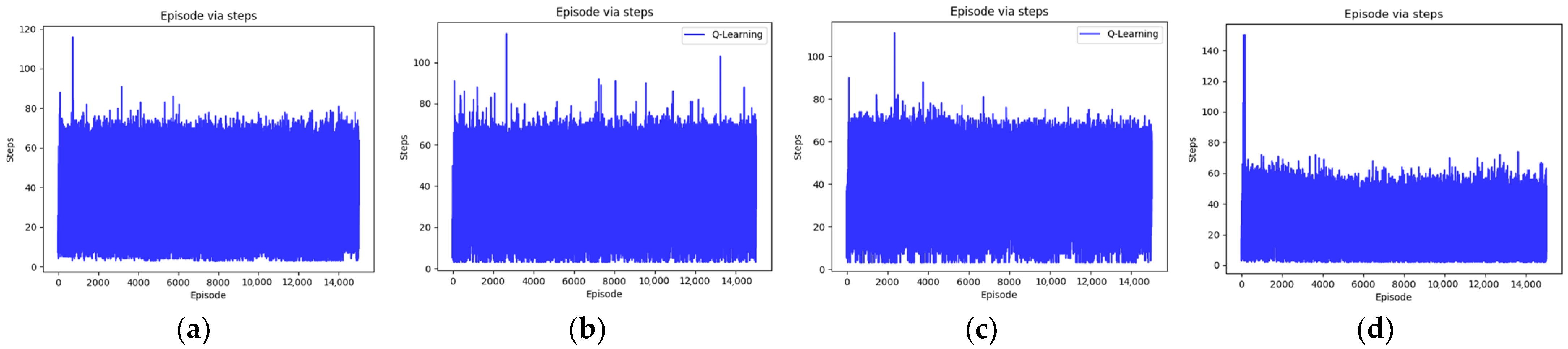
Comparison of Step Counts between the Q-learning Algorithm and the Proposed Algorithm in the Simple Obstacle Environment: (a) Q-learning; (b) AEG-QL; (c) TAR-RL; (d) DRQL.
Figure 7.
Comparison of Step Counts between the Q-learning Algorithm and the Proposed Algorithm in the Complex Obstacle Environment: (a) Q-learning; (b) AEG-QL; (c) TAR-RL; (d) DRQL.
Figure 8.
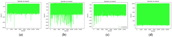
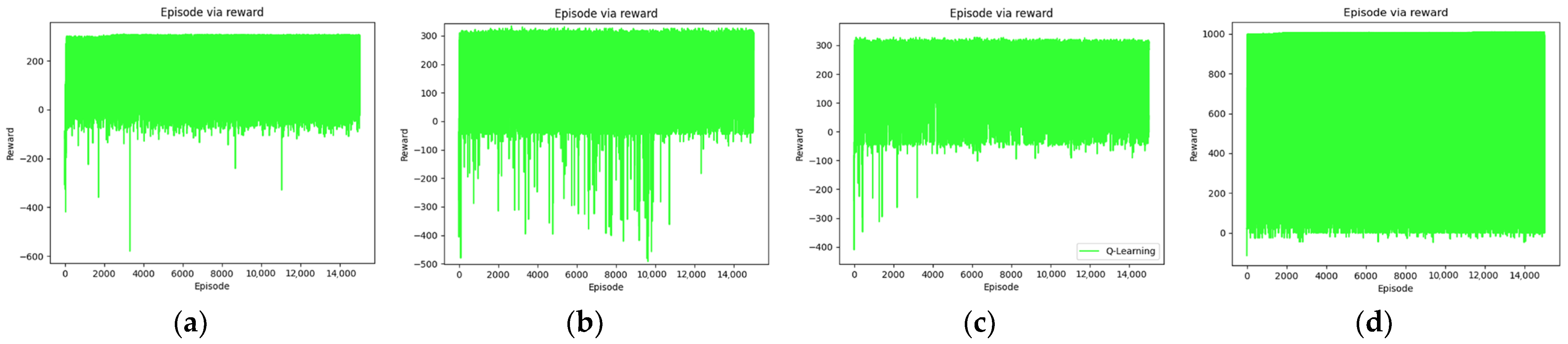
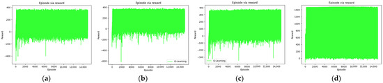
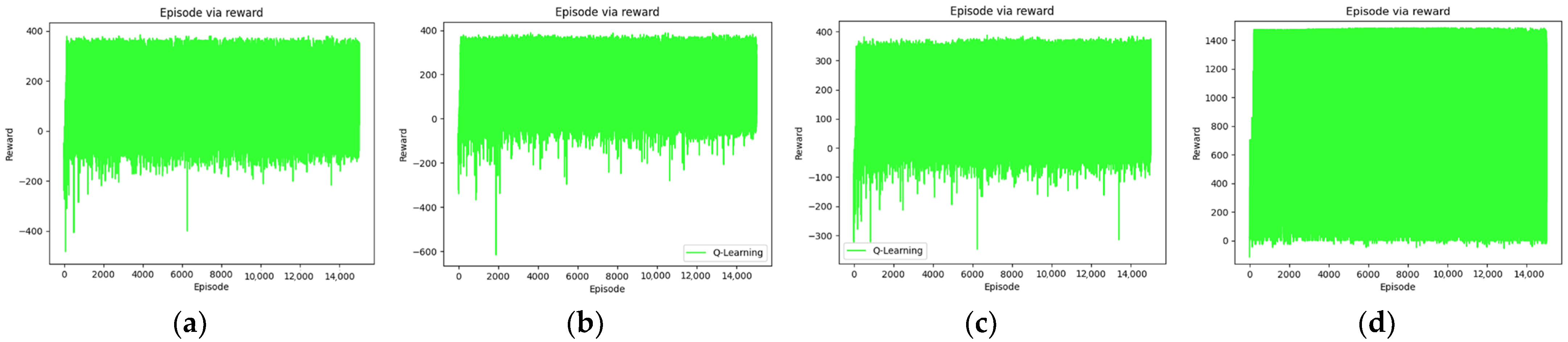
Comparison of Reward Values between the Q-learning Algorithm and the Proposed Algorithm in the Simple Obstacle Environment: (a) Q-learning; (b) AEG-QL; (c) TAR-RL; (d) DRQL.
Figure 9.
Comparison of Reward Values between the Q-learning Algorithm and the Proposed Algorithm in the Complex Obstacle Environment: (a) Q-learning; (b) AEG-QL; (c) TAR-RL; (d) DRQL.
The experiment compares the performance of four algorithms in the hazardous material transportation path planning task. The path planning results using the Q-learning algorithm are shown in Figure 4a, Figure 5a, Figure 6a, Figure 7a, Figure 8a and Figure 9a. The AEG-QL (adaptive dynamic ε-greedy strategy) algorithm is presented in Figure 4b, Figure 5b, Figure 6b, Figure 7b, Figure 8b and Figure 9b. The proposed TAR-RL algorithm, which combines the adaptive dynamic ε-greedy strategy and RUDDER reward redistribution, is shown in Figure 4c, Figure 5c, Figure 6c, Figure 7c, Figure 8c and Figure 9c. Finally, the DRQL algorithm, which integrates a dynamic reward mechanism, is illustrated in Figure 4d, Figure 5d, Figure 6d, Figure 7d, Figure 8d and Figure 9d.
From Figure 4 and Figure 5, it can be observed that both the Q-learning algorithm and the proposed TAR-RL algorithm successfully plan the optimal path in two different obstacle environments, as defined in the experiment. In the simple obstacle environment, the path length for both algorithms is 38, while in the complex obstacle environment, the path length is 58, both representing the shortest paths. In contrast, the DRQL algorithm, which employs an action space with eight directions (up, down, left, right, and diagonal), causes the agent to travel almost along the diagonal. As a result, the shortest path length in the simple obstacle environment is 23, and in the complex obstacle environment, it is 42. In both the simple and complex obstacle environments, it is evident that the TAR-RL algorithm effectively avoids high-risk cells.
Figure 6, Figure 7, Figure 8 and Figure 9 in the experiment visually present the trends of the agent’s steps and rewards as they vary with the training episodes, which are used to evaluate the convergence speed and training stability of each algorithm.
In terms of convergence speed, the step and reward curves clearly show that TAR-RL converges the fastest. In the 20 × 20 simple map, as shown in Figure 6 and Figure 8, the step curve drops rapidly to near 40 steps within just a few thousand episodes, approaching the optimal 38 steps, while the average reward curve also rises quickly from low values to near the maximum positive reward. In the 30 × 30 complex map, as shown in Figure 7 and Figure 9, TAR-RL again leads in reducing the step count to the optimal 58 steps and accumulates positive rewards within the fewest episodes.
The DRQL algorithm, benefiting from dynamic rewards, enters the optimal step range earlier than AEG-QL, with its reward curve turning positive and rising just after TAR-RL. In contrast, although AEG-QL outperforms traditional Q-learning, it still requires more episodes in the middle to late training stages to reduce the step count to the 40–60 range, with rewards lagging behind DRQL. Meanwhile, the basic Q-learning algorithm stays in high step counts and low rewards for a long time in both environments, only slowly converging towards the optimal range in the later stages of training.
Overall, TAR-RL achieves the highest-quality policy with the fewest training episodes in both types of maps, followed by DRQL, AEG-QL, and then Q-learning, which converges the slowest.
In terms of training stability, analysis of the curve fluctuations and peak frequencies reveals that the step and reward curves of TAR-RL are almost flat and free of jitter after convergence, with the smallest variance, indicating that the policy becomes highly stable once converged. DRQL, in both map environments, shows step and reward curves that have largely converged, with only slight and low-frequency oscillations, demonstrating better stability than AEG-QL. Although AEG-QL significantly reduces fluctuations caused by exploration, occasional step increases and reward sawtooth patterns still appear, placing its stability in the middle range. In contrast, the basic Q-learning algorithm continues to experience frequent step peaks and severe reward fluctuations in both the 20 × 20 and 30 × 30 environments during the later stages, suggesting that its policy is easily disrupted by random exploration or environmental complexity.
Thus, the synergy between the RUDDER reward redistribution and the adaptive dynamic ε-greedy strategy enables TAR-RL to not only converge rapidly but also reliably stabilize the optimal path in dynamic environments, significantly enhancing the robustness and consistency of the policy.
The comparison of the success rate and average reward values between the proposed TAR-RL algorithm, AEG-QL, traditional Q-learning, and DRQL algorithms is presented in Table 2.
Table 2.
Algorithm Performance Analysis.
Table 2 reports Success Rate (SR) and Average Reward, which jointly characterize safety under our environment design. SR measures the reliability of achieving a goal without ultimately failing, while average reward penalizes unsafe outcomes. Therefore, higher SR together with higher Average Reward indicates that the agent not only reaches the goal more often but also avoids severe safety violations more effectively.
In the simple obstacle environment, the traditional Q-learning algorithm achieved a success rate of 72.11% and an average reward of 192.09. With the introduction of the adaptive dynamic ε-greedy strategy, the AEG-QL algorithm improved the success rate to 74.75% and the average reward to 226.34. In comparison, the proposed TAR-RL algorithm further increased the success rate to 80.34% and the average reward to 244.24, representing an improvement of 8.23 percentage points and 52.15 reward units over Q-learning, and a significant gain over AEG-QL, with an increase of approximately 5.6 percentage points in success rate and 17.9 in reward value.
In contrast, the DRQL algorithm achieved a success rate of only 64.74%, yet the average reward was as high as 780.01. This discrepancy can be attributed to the misalignment between the reward shaping in the algorithm and the task objectives, where the scale of progress terms is too large and lacks discounting and normalization. As a result, the agent accumulates a large number of positive rewards simply by oscillating around the goal or in the vicinity of obstacles.
These results indicate that, in environments with sparse obstacles and relatively simple settings, TAR-RL is more effective in balancing exploration and exploitation, converging rapidly to a high-quality policy.
In the complex obstacle environment, both the number and complexity of obstacles increase significantly, causing a sharp decline in the success rate of Q-learning to 36.80%, with the average reward dropping to only 108.09. The AEG-QL algorithm improves the success rate to 41.04% and the average reward to 147.48, but it still performs relatively weakly. In contrast, the TAR-RL algorithm stands out in this more challenging environment, achieving a success rate of 59.63% and an average reward of 199.50, representing increases of 22.83 percentage points and 91.41 reward units over Q-learning, and improvements of 18.59 percentage points and 52.02 reward units over AEG-QL. The DRQL algorithm, on the other hand, achieves a success rate of 31.40%, with an unusually high average reward of 827.23. This discrepancy can be attributed to the weak penalties for per-step costs and repeated visits, coupled with overly stringent terminal conditions, which allow the agent to accumulate high rewards even in failed episodes, resulting in a lower success rate.
These results demonstrate that TAR-RL maintains high exploration efficiency and robust policy performance in complex environments, significantly enhancing the agent’s task completion rate and overall return.
Overall, whether in simple or complex environments, TAR-RL significantly outperforms both the traditional Q-learning and AEG-QL algorithms, with a higher success rate than the DRQL algorithm as well. Not only does it achieve a higher success rate, but it also shows a clear advantage in terms of average reward, fully demonstrating the effectiveness and superiority of the proposed algorithm in accelerating convergence and improving task completion quality.
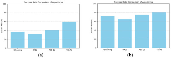
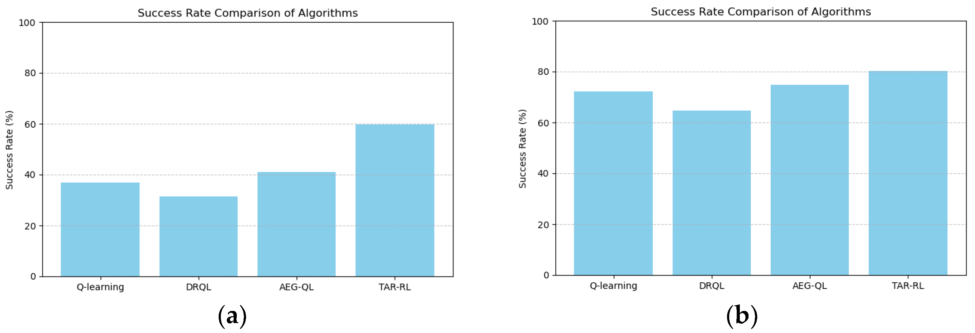
A comparison of success rates between the proposed TAR-RL algorithm, the adaptive AEG-QL algorithm, DRQL algorithm, and the traditional Q-learning algorithm is shown in Figure 10.
Figure 10.
Comparison of Results Between Different Algorithms: (a) Simple Obstacle Environment; (b) Complex Obstacle Environment.
As shown in Figure 10, there is a clear difference in the success rates of the four algorithms across two grid environments with varying levels of complexity.
In the simple obstacle environment, all algorithms achieve relatively high success rates, with a gradual increase in success rate as the algorithms are improved. The traditional Q-learning algorithm has a success rate of 72.11%, while the DRQL algorithm, which incorporates a dynamic reward mechanism, shows a decrease to 64.74%, although it finds the shortest path. The proposed AEG-QL algorithm, which introduces the adaptive dynamic ε-greedy strategy, improves the success rate to 74.75%. Furthermore, the TAR-RL algorithm, which adds the multi-head attention mechanism and RUDDER reward redistribution to AEG-QL, reaches the highest success rate of 80.34%. This significant improvement over the baseline algorithms demonstrates that the TAR-RL algorithm provides stable and effective performance enhancement, even in simple environments.
In the complex obstacle environment, the overall success rate decreases, reflecting the challenge posed by environmental complexity on algorithm performance. Specifically, the success rate of Q-learning drops to 36.80%, the DRQL algorithm achieves a success rate of 31.40%, and the AEG-QL algorithm reaches 41.04%. However, the TAR-RL algorithm still performs the best, with a success rate of 59.63%. Although all algorithms show lower success rates in the complex environment, TAR-RL significantly outperforms the others, demonstrating that the proposed method possesses stronger robustness and adaptability in handling more challenging environments.
The experimental results validate that the proposed TAR-RL algorithm consistently performs well across environments with varying complexity, particularly showcasing a significant advantage in the complex obstacle environment. This improvement not only enhances the success rate of the task but also increases the practicality of the algorithm, proving its effectiveness and superiority in reinforcement learning-based path planning tasks.
4.3. Ablation Study
To clarify the individual contributions of each component in TAR-RL, we conduct an ablation study in both the 20 × 20 and 30 × 30 grid environments under the same protocol as Section 4.1. We evaluate four variants: (i) FULL TAR-RL, (ii) TAR-RL without RUDDER reward redistribution, (iii) TAR-RL without dynamic adaptive ε strategy, and (iv) TAR-RL using a non-attention return predictor (LSTM-only) for the RUDDER module. The ablation results are summarized in Table 3.
Table 3.
Ablation Study of TAR-RL.
Ablation results in Table 3 show that removing any component consistently reduces TAR-RL performance in both environments. On the Simple Obstacle Map, the full model achieves the highest success rate of 80.34% and the highest average reward of 244.24. Removing RUDDER decreases the success rate to 74.75% and the average reward to 226.34. Disabling the dynamic adaptive ε strategy further lowers the success rate to 74.31% and the average reward to 214.53. Replacing the attention-based return predictor with a non-attention predictor also degrades performance, with a success rate of 76.19% and an average reward of 219.65.
The performance gaps are larger on the Complex Obstacle Map. The full model reaches a success rate of 59.63% and an average reward of 199.50. Without RUDDER, the success rate drops to 41.04% and the average reward to 147.48. Disabling dynamic adaptive ε strategy leads to the largest decline, with a success rate of 36.03% and an average reward of 106.24. Removing attention similarly reduces performance, yielding a success rate of 37.32% and an average reward of 109.75. These results indicate that the modules are complementary, and that dynamic adaptive ε strategy regulation and accurate return prediction are especially important in the more challenging environment.
5. Conclusions
This paper addresses the challenges of complex environments, sparse rewards, and high safety requirements in hazardous material transportation path planning by proposing an improved reinforcement learning algorithm, TAR-RL. Built upon traditional Q-learning, the algorithm designs an adaptive dynamic ε-greedy exploration strategy based on the trend of Q-value changes, allowing for dynamic adjustment of the exploration rate according to policy variations, thus improving learning efficiency. By incorporating the RUDDER reward redistribution mechanism, the algorithm performs causal decomposition of delayed rewards, enhancing the learning signals at critical decision points. Additionally, a multi-head attention mechanism is introduced to model the long-term dependencies between state–action pairs, improving the accuracy of reward predictions. The algorithm also integrates an intrinsic reward mechanism to motivate the agent to explore proactively, facilitating self-driven learning. The data that support the findings of this study are available from the corresponding author upon reasonable request.
To support safety-aware hazardous materials transportation, we design a risk-aware routing formulation that discourages entering high-risk regions while maintaining efficient goal-directed navigation. Experimental comparisons in environments with varying obstacle complexities demonstrate that TAR-RL outperforms both traditional Q-learning and the improved algorithms in terms of convergence speed, success rate, and training stability, particularly exhibiting strong robustness and adaptability in complex environments. Overall, TAR-RL effectively enhances the intelligence and practical value of hazardous material transportation path planning, providing strong support for further application of reinforcement learning algorithms in complex real-world scenarios.
Limitations and Future Work
The present study validates TAR-RL in two deterministic grid environments (20 × 20 and 30 × 30) under a single-agent routing setting, using risk-aware terminal penalties and a fixed maximum step budget. This configuration provides a controlled, route-level abstraction of HAZMAT safety via a static risk map; however, it does not explicitly capture uncertainty arising from human behavior, perception errors, or time-varying cognitive risk encountered in real operations. In addition, time-window constraints, fleet-level coordination (e.g., platooning), and multi-objective scheduling on continuous road networks are beyond the scope of the current experiments and are therefore not modeled. Future work will extend TAR-RL to probabilistic and dynamic risk maps, incorporate interaction-aware runtime safety layers, and apply the framework to fleet/platoon settings with coordinated routing and scheduling (e.g., platoon-aware cooperative control such as CACC). In addition, future work will investigate continuous-space and road-network representations through multi-resolution discretization, graph-based MDP formulations, and function approximation to support larger-scale and more realistic HAZMAT transportation scenarios.
Author Contributions
Conceptualization, K.C., H.J. and H.W.; Methodology, K.C. and M.G.; Software, M.Y.; Validation, K.C., H.J. and J.G.; Formal analysis, M.G., M.Y. and H.W.; Investigation, K.C., M.G. and J.G.; Resources, K.C. and H.J.; Data curation, M.Y. and J.G.; Writing—original draft, K.C.; Writing—review & editing, K.C., H.J. and H.W.; Visualization, M.Y.; Supervision, K.C. and H.J.; Project administration, H.W.; Funding acquisition, K.C. and H.J. All authors have read and agreed to the published version of the manuscript.
Funding
This work was supported by the Institute of Information & Communications Technology Planning & Evaluation (IITP)—Innovative Human Resource Development for Local Intellectualization program grant funded by the Korea government (MSIT) (IITP-2026-RS-2022-00156334, contribution rate: 70%) and Liaoning Provincial Department of Science and Technology Plan Project—General Project (Project No.: 2025-MS-141).
Data Availability Statement
The code and simulation environment used in this study (including the deterministic obstacle/high-risk cell layouts) and the training/evaluation logs supporting the reported results are available from the corresponding author upon reasonable request. No external datasets were used in this work.
Acknowledgments
The authors would like to express their sincere gratitude to all the institutions and organizations that provided support and funding for this research. Special thanks to them for their generous financial sponsorship, which made this study possible. We also appreciate the insightful feedback and suggestions provided by the anonymous reviewers, which greatly contributed to improving the quality of this work. Finally, we extend our gratitude to all those who contributed to the successful completion of this research. Their invaluable assistance and encouragement have been instrumental throughout the study.
Conflicts of Interest
The authors declare no conflicts of interest. The funders had no role in the design of the study.
Abbreviations
| TAR-RL | Trend-Aware and Attention-Augmented Reward Redistribution Reinforcement Learning |
| AEG-QL | adaptive dynamic ε-greedy strategy |
| DRQL | dynamic reward-enhanced Q-learning |
References
- Sun, Y.; Huang, P.; Cao, Y.; Jiang, G.; Yuan, Z.; Bai, D.; Liu, X. Multi-Objective Optimization Design of Ladle Refractory Lining Based on Genetic Algorithm. Front. Bioeng. Biotechnol. 2022, 10, 900655. [Google Scholar] [CrossRef] [Scilit] [PubMed]
- Zhang, X.; Xiao, F.; Tong, X.; Yun, J.; Liu, Y.; Sun, Y.; Tao, B.; Kong, J.; Xu, M.; Chen, B. Time Optimal Trajectory Planing Based on Improved Sparrow Search Algorithm. Front. Bioeng. Biotechnol. 2022, 10, 852408. [Google Scholar] [CrossRef] [Scilit] [PubMed]
- Kuo, R.J.; Luthfiansyah, M.F.; Masruroh, N.A.; Zulvia, F.E. Application of Improved Multi-Objective Particle Swarm Optimization Algorithm to Solve Disruption for the Two-Stage Vehicle Routing Problem with Time Windows. Expert Syst. Appl. 2023, 225, 120009. [Google Scholar] [CrossRef] [Scilit]
- Dai, Z.; Zhang, Z.; Chen, M. The Home Health Care Location-Routing Problem with a Mixed Fleet and Battery Swapping Stations Using a Competitive Simulated Annealing Algorithm. Expert Syst. Appl. 2023, 228, 120374. [Google Scholar] [CrossRef] [Scilit]
- Huang, H.; Cheng, H.; Zhou, Z.; Wang, Z.; Wang, H.; Liu, Q.; Li, X. REACT: Runtime-Enabled Active Collision-Avoidance Technique for Autonomous Driving. Adv. Eng. Inform. 2026, 71, 104248. [Google Scholar] [CrossRef] [Scilit]
- Li, S.; Xu, X.; Zuo, L. Dynamic Path Planning of a Mobile Robot with Improved Q-Learning Algorithm. In Proceedings of the 2015 IEEE International Conference on Information and Automation, Lijiang, China, 8–10 August 2015; pp. 409–414. [Google Scholar]
- Fang, W.; Liao, Z.; Bai, Y. Improved ACO Algorithm Fused with Improved Q-Learning Algorithm for Bessel Curve Global Path Planning of Search and Rescue Robots. Robot. Auton. Syst. 2024, 182, 104822. [Google Scholar] [CrossRef] [Scilit]
- Li, D.; Yin, W.; Wong, W.E.; Jian, M.; Chau, M. Quality-Oriented Hybrid Path Planning Based on A* and Q-Learning for Unmanned Aerial Vehicle. IEEE Access 2021, 10, 7664–7674. [Google Scholar] [CrossRef] [Scilit]
- Hu, L.; Wei, C.; Yin, L. Fuzzy A∗ Quantum Multi-Stage Q-Learning Artificial Potential Field for Path Planning of Mobile Robots. Eng. Appl. Artif. Intell. 2025, 141, 109866. [Google Scholar] [CrossRef] [Scilit]
- Zhang, T.; Mo, H. Reinforcement Learning for Robot Research: A Comprehensive Review and Open Issues. Int. J. Adv. Robot. Syst. 2021, 18, 17298814211007305. [Google Scholar] [CrossRef] [Scilit]
- Zanette, A.; Wainwright, M.J. Bellman Residual Orthogonalization for Offline Reinforcement Learning. Adv. Neural Inf. Process. Syst. 2022, 35, 3137–3151. [Google Scholar]
- Clifton, J.; Laber, E. Q-Learning: Theory and Applications. Annu. Rev. Stat. Its Appl. 2020, 7, 279–301. [Google Scholar] [CrossRef] [Scilit]
- dos Santos Mignon, A.; de Azevedo da Rocha, R.L. An Adaptive Implementation of ε-Greedy in Reinforcement Learning. Procedia Comput. Sci. 2017, 109, 1146–1151. [Google Scholar] [CrossRef] [Scilit]
- Sutton, R.S.; Mahmood, A.R.; White, M. An Emphatic Approach to the Problem of Off-Policy Temporal-Difference Learning. J. Mach. Learn. Res. 2016, 17, 1–29. [Google Scholar]
- Blain, B.; Sharot, T. Intrinsic Reward: Potential Cognitive and Neural Mechanisms. Curr. Opin. Behav. Sci. 2021, 39, 113–118. [Google Scholar] [CrossRef] [Scilit]
- Dokmanic, I.; Parhizkar, R.; Ranieri, J.; Vetterli, M. Euclidean Distance Matrices: Essential Theory, Algorithms, and Applications. IEEE Signal Process. Mag. 2015, 32, 12–30. [Google Scholar] [CrossRef] [Scilit]
- Arjona-Medina, J.A.; Gillhofer, M.; Widrich, M.; Unterthiner, T.; Brandstetter, J.; Hochreiter, S. Rudder: Return Decomposition for Delayed Rewards. In Advances in Neural Information Processing Systems 32, Proceedings of the NeurIPS 2019, Vancouver, BC, Canada, 8–14 December 2019; Wallach, H., Larochelle, H., Beygelzimer, A., d’Alché-Buc, F., Fox, E., Garnett, R., Eds.; NeurIPS: San Diego, CA, USA, 2019. [Google Scholar]
- Jin, P.; Zhu, B.; Yuan, L.; Yan, S. MoH: Multi-Head Attention as Mixture-of-Head Attention 2025. arXiv 2025, arXiv:2410.11842. [Google Scholar]
- Zhou, D.; Du, X.; Liu, S.; Su, Q.; Guo, H. Research on LSTM-Driven UAV Path Planning. In Proceedings of the Fourth International Conference on Advanced Algorithms and Neural Networks (AANN 2024), Qingdao, China, 9–11 April 2024; Volume 13416, pp. 910–917. [Google Scholar]
- Goyal, P.; Dollár, P.; Girshick, R.; Noordhuis, P.; Wesolowski, L.; Kyrola, A.; Tulloch, A.; Jia, Y.; He, K. Accurate, Large Minibatch SGD: Training ImageNet in 1 Hour 2018. arXiv 2018, arXiv:1706.02677. [Google Scholar]
- Gharbi, A. A Dynamic Reward-Enhanced Q-Learning Approach for Efficient Path Planning and Obstacle Avoidance in Mobile Robotics. Appl. Comput. Inform. 2024. [Google Scholar] [CrossRef] [Scilit]

Disclaimer/Publisher’s Note: The statements, opinions and data contained in all publications are solely those of the individual author(s) and contributor(s) and not of MDPI and/or the editor(s). MDPI and/or the editor(s) disclaim responsibility for any injury to people or property resulting from any ideas, methods, instructions or products referred to in the content. |
© 2026 by the authors. Licensee MDPI, Basel, Switzerland. This article is an open access article distributed under the terms and conditions of the Creative Commons Attribution (CC BY) license.