An Improved Carbon Dioxide Monitoring Method Related to China’s Carbon Emissions Trading System in Cement Plants

Abstract

The cement industry will be officially regulated by China’s national carbon market. Authenticity and accuracy of emission data are prerequisites and the foundation for ensuring the healthy and stable operation of the market. At present, China’s carbon market mainly adopts the Calculation-Based Method (CBM) for data accounting. However, in the cement sector, this method faces challenges due to the inherent complexity of both raw materials and fuels, making it difficult to obtain accurate emission data through CBM alone. Therefore, regulatory authorities are promoting the installation and application of the Continuous Emission Monitoring System (CEMS) by enterprises. Pilot studies, however, have revealed considerable discrepancies between the data from the two methods. In this study, a combined data monitoring and accounting method was proposed, in which CBM and CEMS were combined to improve emission data quality. The actual operational and emission data from a case enterprise was taken as an example, and this study conducted systematic analysis and research on data collection and preprocessing, operating condition classification, correlation model construction, and abnormal data diagnosis. The results revealed that this combined method can effectively improve the degree of correlation between CBM and CEMS carbon emissions. Moreover, higher accuracy of abnormal data identification can be achieved through statistical testing. This combined monitoring method not only strengthens data tamper-resistance at the enterprise level but also has the potential to reduce regulatory oversight costs, thereby providing reliable technical support for emission data quality control.

1. Introduction

The cement industry is one of the world’s largest consumers of energy and sources of CO₂ emissions, with China alone accounting for approximately 52% of the sector’s global carbon footprint [1,2]. In 2020, the CO₂ emissions of China’s cement industry were slightly higher than 1.3 billion tons [3], ranking behind the power and steel sectors. Among them, the CO₂ emissions generated from cement production accounted for about 90% of the total cement industry emissions [4]. Given the scale of production, the low-carbon transition of China’s cement industry is indispensable for achieving the national carbon neutrality target by 2060.

In March 2025, the Ministry of Ecology and Environment issued the Work Plan of National Carbon Emissions Trading Market Covering Steel, Cement, and Aluminum Smelting Industries [5], which formally included the three industries of steel, cement, and aluminum smelting in the regulation of the national carbon emissions trading market. As the world’s largest greenhouse gas emissions trading market [6], China’s carbon market has demonstrated its potential to reduce corporate emissions while supporting economic growth [7,8] and has made remarkable progress in improving policies, invigorating transactions, expanding coverage, improving data quality, and encouraging corporate behavior.

Data quality is fundamental to the effective implementation of environmental policies and the sound functioning of the carbon market, yet carbon emission data is inherently vulnerable to misreporting and manipulation [9,10]. Accurate carbon emission data is conducive to the government promptly identifying problems with the carbon emission data of industries and effectively preventing illegal and irregular behaviors such as false reporting, under-reporting, and fraud of carbon emission data [11]. Carbon accounting methodologies directly shape the reliability and comparability of reported emissions, ultimately undermining market credibility and regulatory effectiveness [12]. China has taken on a number of measures. In September 2024, Guidelines for Accounting and Reporting of Greenhouse Gas Emissions of Enterprises in Cement Industry [13] was issued to simplify the key parameters of the accounting process and further improved the operability of the method.

The main methods for carbon emission accounting include the Calculation-Based Method (CBM) and the Continuous Emission Monitoring System (CEMS) [14,15]. The CBM estimates carbon emissions based on activity data and emission factors, which heavily rely on manual data collection and on-site measurements [16]. CEMS directly monitors flow rate, gas concentration, and other parameters through sensors and analytical instruments, requiring less human intervention and enabling real-time and automatic monitoring of carbon emissions from fixed emission sources. Although many regions, including Europe, have long relied on and encouraged the use of CBM and only recommended the application of CEMS in some large cement clinker production lines or facilities with a high share of alternative fuels. Since the fuel types and raw meal compositions in the cement industry remain highly heterogeneous, it is increasingly difficult to achieve high data accuracy through CBM alone [17].

The management department in China has clearly put forward a plan to innovate the accounting methods and promote industrial enterprises to install online monitoring equipment, CEMS, and the pilot application. In 2024, in the Notice on the Action Plan for Further Strengthening the Construction of Standard Measurement System for Carbon Peak and Carbon Neutrality (2024–2025) [18] and The Work Plan for Improving the Statistical Accounting System of Carbon Emissions [19], it was particularly mentioned to promote the research on carbon measurement technologies in key industries such as power, steel, and cement; to conduct comparative studies on direct measurement methods and accounting methods; and to encourage pilot projects and promote the application, which provides clear policy guidance for the cement industry to carry out carbon emission monitoring.

However, the literature indicates deviations between carbon emission results calculated using CBM and CEMS methods. Unreliable data under irregular conditions and improper installation or calibration could affect the data quality of CEMS [20,21]. By October 2024, 72 enterprises in China’s power, steel, and cement industries have installed 152 CEMS [22]. For nearly 90% of coal-fired units in power sector pilots, the annual deviation between CEMS and CBM results was within ±10%. Historical cumulative data comparisons outperformed those based on individual months [23]. For a certain cement enterprise in China, with a credible probability of 95%, the fluctuation range of the CBM emission could be as high as 36%, while the fluctuation range of CEMS data was only about 10% [24]. For U.S. power plants, the overall emissions differences between the two methods were relatively small (3.5% for total output and 2.3% for electricity-only). However, at the individual facility level, the average discrepancies were significantly larger, reaching 16.9% and 25.3%, respectively [25]. Quick (2014) reported an estimation deviation of ±10.8% between the two methods for 210 coal-fired power units [26]. Lee (2014) showed that CO₂ emissions of a bituminous coal-fired heat supply utility calculated by CBM were 12–19% lower than those by CEMS [27]. Meanwhile, illegal shutdowns or improper operation of manual accounting systems or monitoring equipment have led to data manipulation or systematic deviations in emission records [28]. Due to the inherent uncertainties of online monitoring, there may be distortion of individual data points. In response to these challenges, improved data monitoring and calculation methods were proposed by identifying the correlation between the two methods [9], which are beneficial for identifying samples with higher risks of data fraud and providing technical support for carbon data quality control.

2. Methodology

2.1. Measurement by CEMS

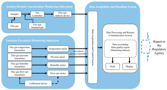
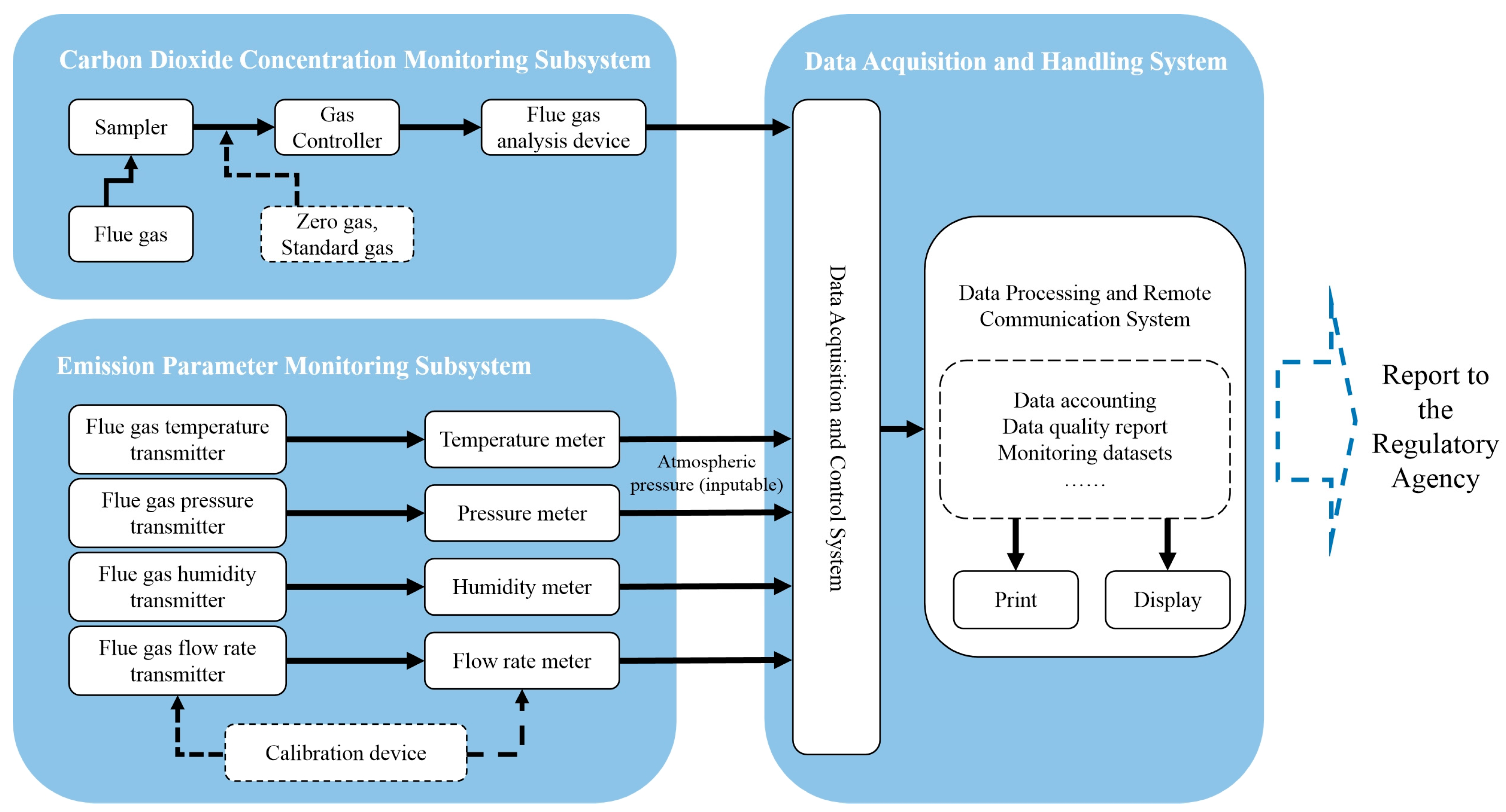
A CEMS integrates sampling, conditioning, analytical components, and supporting software, aiming to continuously measure flue gas parameters through real-time analysis of representative gas streams. By relying on automated and instrument-based measurements, CEMS enables real-time monitoring of CO₂ emissions from stationary sources. As illustrated in Figure 1 [29], the CO₂-CEMS deployed in this study consisted of three major subsystems: a CO₂ concentration monitoring subsystem, a flue gas parameter subsystem, and a data acquisition and handling system (DAHS).

Figure 1. Schematic diagram of the CO₂-CEMS composition. (Solid arrows represent material and information paths within the system, whereas dashed arrows indicate auxiliary or non-continuous paths outside the core system boundary.

The monitored parameters included the actual flue gas flow rate, CO₂ concentration (dry basis), temperature, static pressure, and humidity. The actual flue gas flow rate was converted to standard dry flow rate by correcting for temperature, pressure, and humidity. In this study, a complete set of online CO₂ monitoring instruments manufactured by SICK MAIHAK GmbH (Waldkirch, Germany) was installed at the tail-end stack of the production line, including ultrasonic flowmeters (FLOWSIC100), a CO₂ analyzer (SMC-9021), a pressure meter (SMC 202 T/P), a temperature meter (SMC 202 T/P), and a humidity meter (SMC 209IC). The installation strictly followed national technical specifications for pollutant CEMS [30], ensuring sufficient straight-pipe sections and representative flow conditions to minimize measurement bias.

2.2. Measurement by CBM

According to the Guideline for Accounting and Reporting of Greenhouse Gas Emissions in the Cement Industry [13], CO₂ emissions from clinker production include two categories: fossil fuel combustion emissions and process emissions. To maintain the consistency between the calculation boundary of CBM and CEMS, this study additionally included carbon emissions generated from the use of coal gangue as an alternative raw material and waste textiles as an alternative fuel. Theoretically, the amount of CO₂ captured can be quantified according to the method stipulated in Technical Specifications for Quantification and Verification of Greenhouse Gas Emission Reductions in Carbon Capture, Utilization and Storage (CCUS) Projects [31]. Since the facility examined in this study does not involve CO₂ capture, the calculated emission of CBM equals the sum of fossil fuel combustion emissions, process emissions including those from alternative raw materials, and emissions from the alternative fuels, as calculated using the following formula (Formula (1)):

$$E_{CBM}=E_{ff}+E_p+E_{af}$$

(1)

where E represents carbon emissions, ff represents fossil fuel combustion, p represents process, and af represents alternative fuels.

Fossil fuel combustion emissions from clinker were calculated as the product of the coal consumption, the lower calorific value of coal, the carbon content per unit of heat input, the carbon oxidation rate, and the molecular-weight ratio of carbon dioxide to carbon.

Process emissions from clinker production equaled the product of clinker output multiplied by the process emission factor minus the product of the consumption of non-carbonate alternative raw materials multiplied by the corresponding deduction coefficient. Clinker was classified into four categories: Portland cement clinker, white Portland cement clinker, sulfoaluminate (ferroaluminate) cement clinker, and aluminate cement clinker. The corresponding process emission factors were 0.535, 0.550, 0.413, and 0.292 tCO₂/t, respectively. Non-carbonate alternative raw materials were categorized into eight categories, each assigned a specific deduction coefficient.

The combustion process emissions from alternative fuels were calculated as the sum of the products of the consumption of each alternative fuel, and its corresponding lower calorific value on a received basis, and the carbon emission factor per unit calorific value [32].

2.3. Combined Monitoring Method

The process workflow of the combined monitoring method was divided into the following steps:

(1)

Data collection and preprocessing.

The accounting boundary and emission sources of the clinker production were first defined. Emission data were then obtained using both CBM and CEMS. At any given timestamp, the CO₂ emissions measured by CEMS and those calculated using CBM did not correspond to the same physical emission event. This discrepancy occurred because CEMS directly measured the CO₂ concentration and flow rate in the stack, whereas emissions calculated by CBM were based on the recorded consumption of fuels and raw meals at weighing devices. A time lag existed between the two monitoring methods due to a certain residence time required for materials—from being weighed to undergoing combustion or calcination, to finally appearing as CO₂ in the flue gas. For fuel combustion, it typically took 1–2 min from the time coal was weighed until CO₂ was measured at the stack. Such minute-scale temporal offsets have a negligible impact on the comparability of the two datasets for a period of time. For raw meal consumption, although the delay was longer, approximately 10–15 min, its consumption was relatively stable. Meanwhile, cement production enterprises exhibit strong operational stability characteristics [33]. Although there was a time lag between CBM and CEMS emission estimates, the overall stability of production implies that lag correction was not needed in this study. The trend of data monitored by CBM and CEMS was relatively consistent in the same period after integrating the second-level data for a certain period of time. In order to ensure a high frequency of data collection, in this study, the second-level emission data were aggregated into 15 min intervals.

(2)

Operating conditions classification and correlation models construction.

To identify the correlation between the two methods, the correlation coefficient was proposed and defined as the ratio of CO₂ emissions calculated by the CBM to the carbon emissions calculated by the CEMS in a 15 min interval. Generally speaking, variations in production load and fuel composition can alter the flue gas flow field, which in turn may affect the accuracy of the CEMS. Therefore, the operating conditions were classified according to production load, fuel composition, and instrument calibration. An essential criterion for the operating condition classification is that, within each operating condition, the correlation coefficients (or emission ratios) exhibit a unimodal and approximately normal distribution. Commonly used unimodality tests include Hartigan’s Dip Test. The mean correlation coefficients under each operating condition were calculated, and a corresponding correlation model between the CBM and CEMS data was established. The correlation model was then applied to adjust the CEMS emissions. In this study, two forms of CEMS data are distinguished: raw CEMS data (CEMS raw) and adjusted CEMS data (CEMS adjusted). The adjusted CEMS data were obtained by multiplying the raw CEMS emissions by the mean correlation coefficients derived under each operating condition. The cumulative error between the CBM emissions and the adjusted CEMS emissions was then evaluated. A successful correlation model was confirmed when the cumulative error was less than or equal to the specified threshold. Otherwise, the classification of operating conditions should be reconsidered.

The correlation coefficient was calculated as follows:

$$R_i={\displaystyle \frac{E_{CBM,i}}{E_{CEMS(raw),i}}}$$

(2)

where i represents the i-th interval of 15 min, R represents the correlation coefficient, and E still represents carbon emissions.

(3)

Abnormal data diagnosis.

The correlation coefficient under consistent operating conditions was assumed to follow a stable statistical distribution, characterized by a constant mean. The principle of abnormal data diagnosis methods is based on the statistical theory of probability distribution consistency. Related methods can be categorized into two approaches: traditional statistical methods (such as hypothesis testing and distribution comparison) and machine learning-based methods (such as anomaly detection algorithms and model-based techniques). In this study, a statistical method was used to compare the correlation coefficient datasets from the test period with those from the reference period. A Bootstrap mean test was used to assess whether a significant difference existed between the mean values of the two datasets. If manipulation or abnormal behavior occurred in either the CBM or CEMS data during the test period, the average correlation coefficient in the test datasets would be expected to shift accordingly, and the corresponding monitoring data would be identified as anomalous.

Because high-frequency datasets containing confirmed manipulation or anomaly events for both CBM and CEMS are currently unavailable, this study simulated anomaly scenarios. The experimental procedure consisted of four steps. First, all correlation coefficient data under a given operating condition were randomly shuffled and split into two non-overlapping sets: the first 40% as the reference datasets and the next 40% as the test datasets. Second, 10% of the test data points were randomly selected and their correlation coefficients were artificially reduced by 2%, 5%, 10%, or 15%. Based on pilots’ experiences, data with deviations greater than 10% will be flagged manually as potentially anomalous [34] or the uncertainty of annual CO₂ emissions from CEMS should be controlled within 10% [35]. The uncertainty in CO₂ emissions by CEMS is 3.9%, while that by CBM is 3.4% in a case study [27]. The range of 2–15% covered the potential range of anomalies that are not easily detected and are chosen to simulate realistic manipulation scenarios, where large deviations are more easily detected. Third, a Bootstrap mean test was conducted. A p-value ≥ 0.05 indicated no significant difference between datasets, while a p-value < 0.05 signaled a potential anomaly or manipulation risk [36]. Finally, to assess the method’s effectiveness and robustness, the entire process—from resampling to testing—was repeated 30 times under each operating condition and manipulation level.

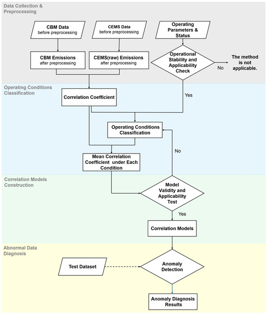
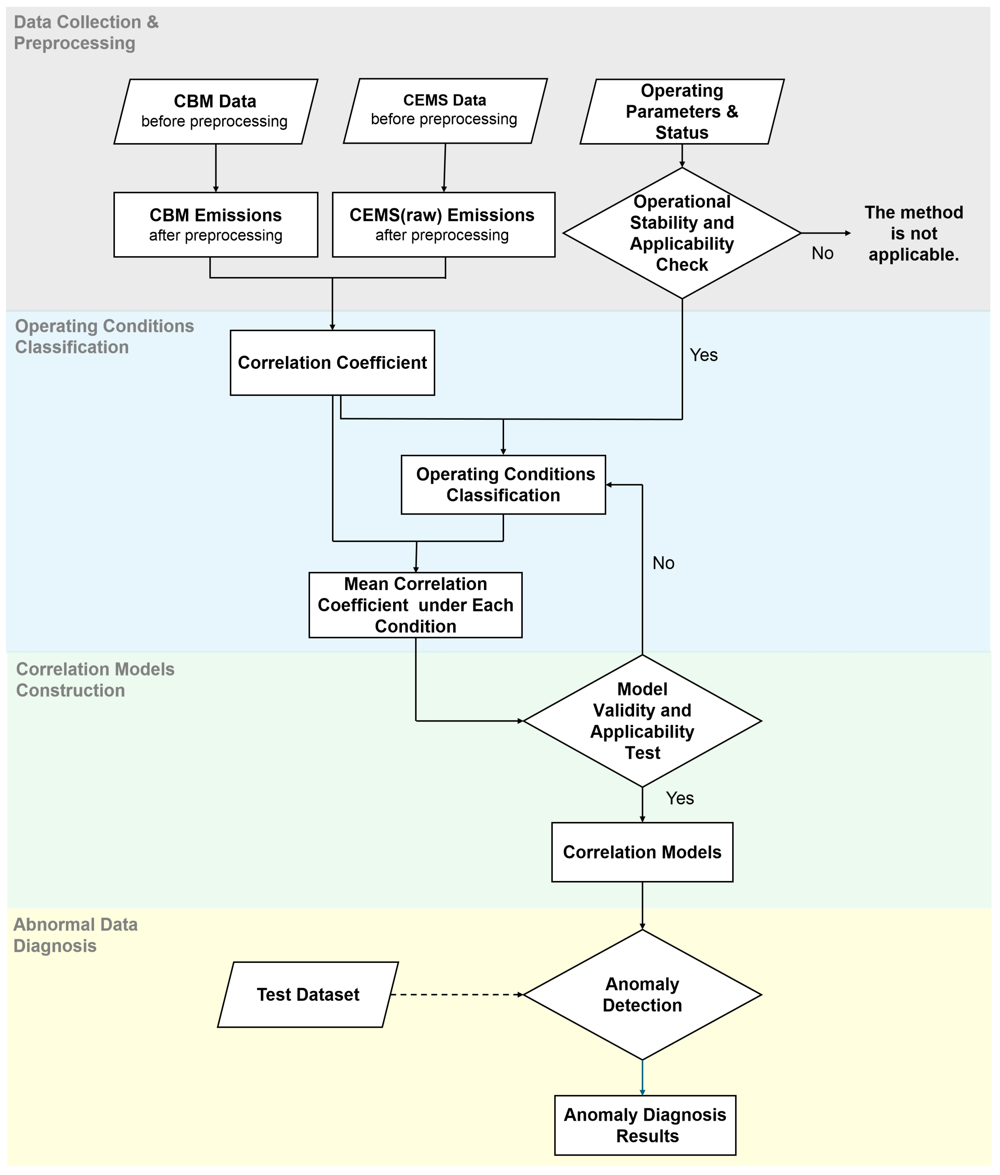
A step-by-step description of the workflow is shown in Figure 2.

Figure 2. The workflow of combined monitoring method.

3. Results and Discussions

3.1. Data Collection and Preprocessing

The data collection for this study was from 12 October 2024 to 25 March 2025. Since single-source monitoring data did not meet the research requirements, this study excluded periods with partial data gaps. Specifically, the duration of missing second-level CBM data accounted for 1.13% of the total period, and the duration of missing second-level CEMS data accounted for 1.06%.

The purpose of data cleaning was to eliminate interfering data. Interfering data was identified using a threshold-based method informed by operational experience: if the measured CO₂ concentration exceeded the reasonable range of 15–40% under normal production conditions, the data were flagged as interference. For humidity, the acceptable range was set between 7% and 100%. Values outside this range were identified as interference. During normal operation, the CO₂ concentration remained stable at approximately 33–34%, and the average humidity was 22%. The above thresholds were selected to exclude data affected by routine calibration with standard dry gases at 0% and 45% CO₂, as well as by maintenance operations such as back purging. During these periods, measured CO₂ concentration and humidity deviated from actual flue gas conditions. The applied thresholds therefore remove such non-representative data while retaining valid measurements under normal operations. Statistical results showed that the proportion of interfering data for concentration and humidity measurement was approximately 0.18% and 0.15%, respectively, with the interference periods largely overlapping.

After data cleaning, carbon emissions were aggregated into 15 min intervals, subject to a strict validity criterion during the aggregation process. Specifically, if more than 75% of the original second-level data within a 15 min interval were either missing or flagged as abnormal, the aggregated emission value for that interval was considered invalid and treated as missing The adoption of 75% is consistent with the requirement of China’s national standard for CEMS in the flue gas emitted from stationary sources [37], which defines valid hourly averages based on at least 75% valid data. The 75% validity threshold provided a pragmatic compromise to balance data representativeness and robustness under practical monitoring constraints.

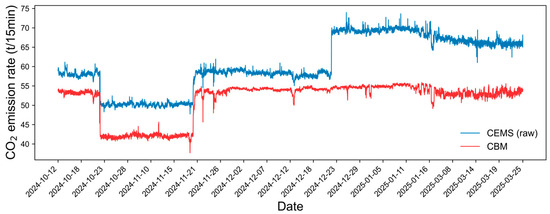
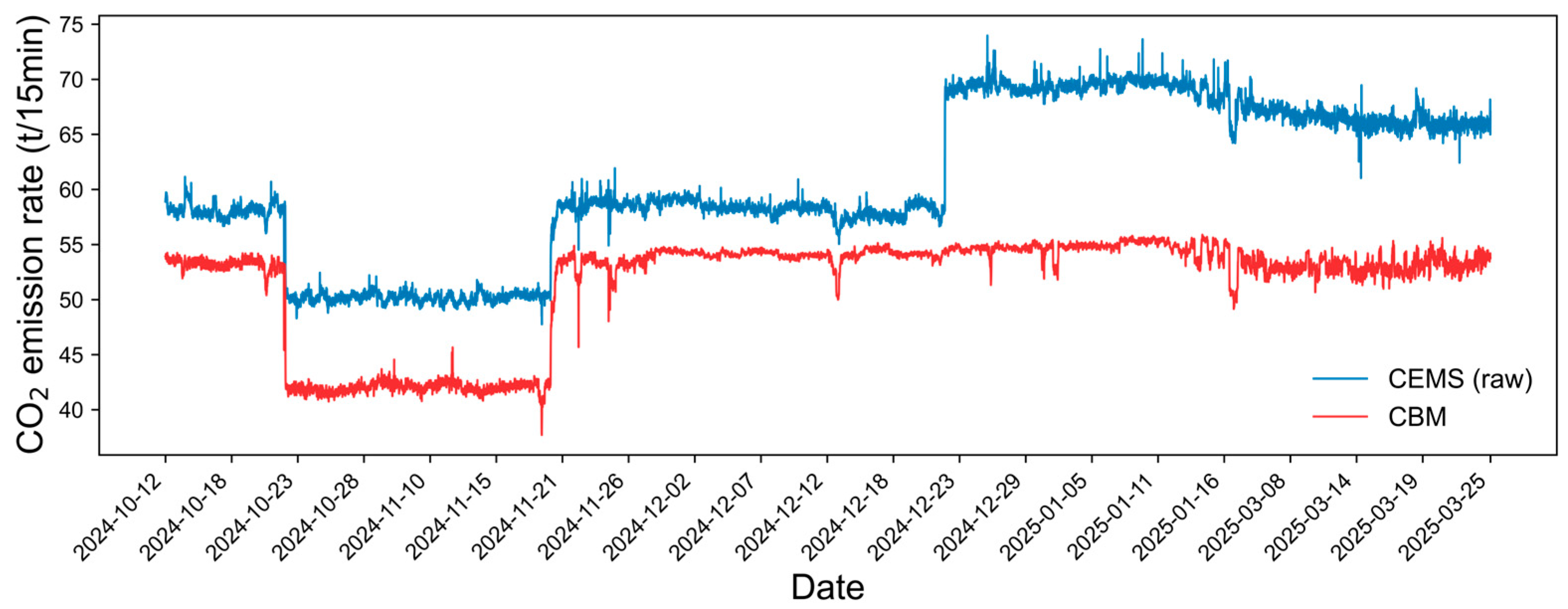
Figure 3 shows the fluctuations in carbon emissions observed at each 15 min interval during the study period. Excluding the sudden spike of CEMS emissions (CEMS (raw)) on 22 December 2024, which was due to humidity meter calibration, the trends of carbon emissions obtained from CEMS and CBM were generally comparable.

Figure 3. Comparison of CO₂ emission rates obtained by CBM and CEMS.

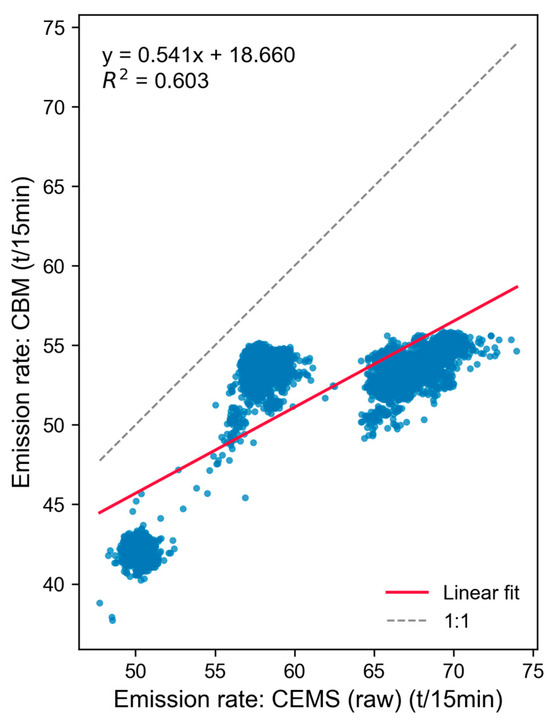
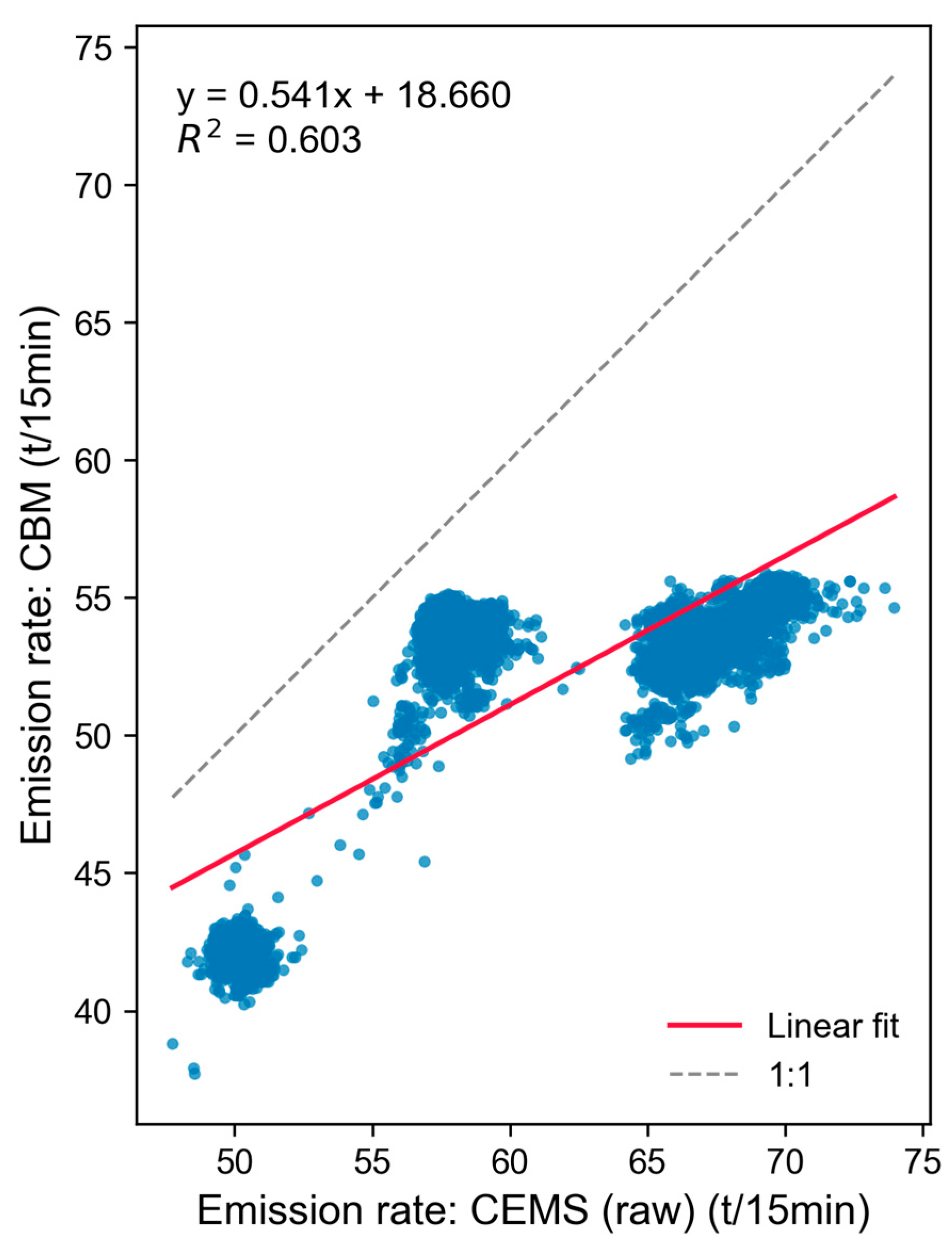
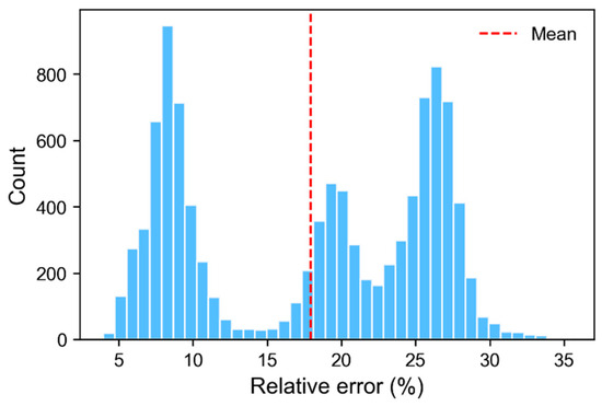
From the consistency analysis of the two original datasets (Figure 4), the Coefficient of Determination (R²) for data fitting was 0.603, indicating a weak correlation and poor consistency between the two datasets. From the perspective of the error distribution (Figure 5), the single-point errors between the two datasets ranged from 5% to 30%, with the total relative error over the entire period being 17.87%. The error histogram displayed three distinct peaks, indicating that the error distribution was concentrated in three separate value ranges.

Figure 4. Consistency assessment between CBM and CEMS (raw) emission data.

Figure 5. Relative error distribution between CBM and CEMS (raw) emissions (CBM as reference).

3.2. Operating Conditions Classification

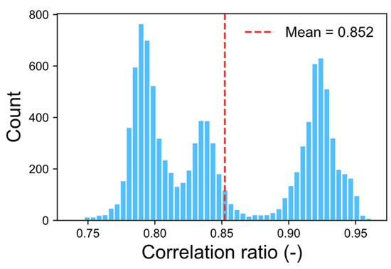
In this study, Hartigan’s Dip Test applied to all correlation coefficients (histograms in Figure 6) yielded a p-value of 0.00000, rejecting unimodality at α = 0.05. Figure 6 shows the statistical distribution of correlation coefficients during the whole experimental period, which exhibits a multimodal distribution. This indicated the trend in data concentration across distinct intervals. Generally speaking, each peak corresponded to a relatively concentrated set of data. The multi-peak distribution of the correlation coefficients indicated that there may be different operating conditions within the entire experimental time frame.

Figure 6. Distribution of correlation coefficients.

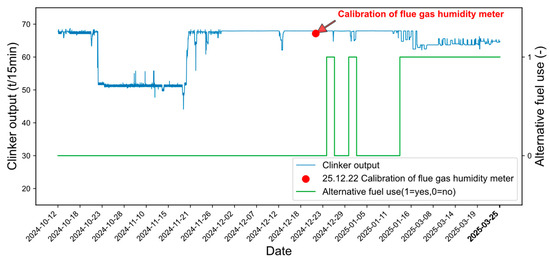
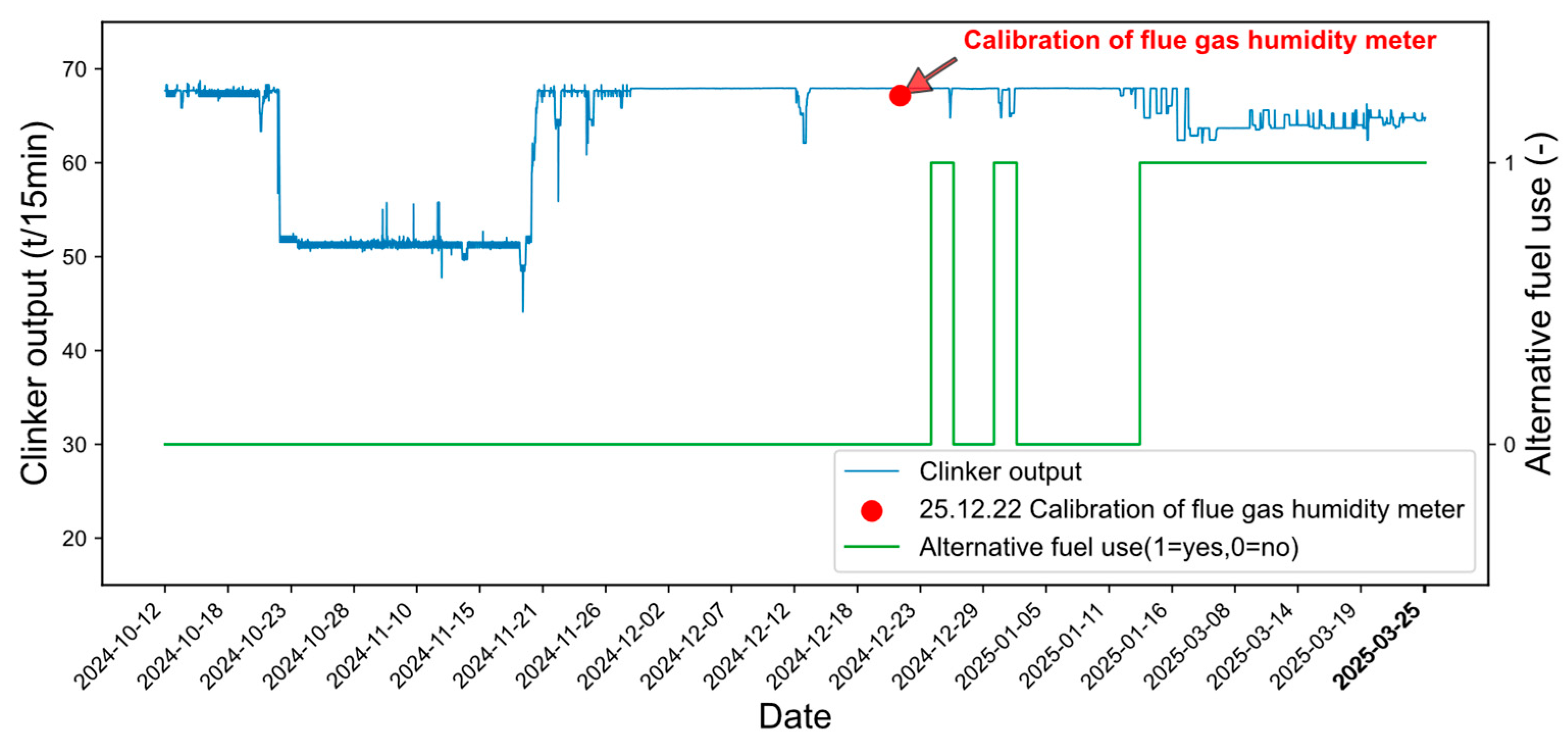
The correlation model construction and abnormal data detection were based on the assumption that the distribution of correlation coefficients should be unimodal and approximately normal under consistent operating conditions. Therefore, it was necessary to identify the key factors influencing the correlation coefficient and to classify operating conditions accordingly. This ensured that the distribution of correlation coefficients under each operation condition approximates a normal distribution. Figure 7 shows the clinker output, alternative fuel usage and instrument calibration records during the experiment period. The data showed dynamic fluctuations in clinker output and alternative fuel consumption, with the humidity meter calibration performed on 22 December.

Figure 7. Overview of operating status: clinker output, alternative fuel use, and instrument calibration.

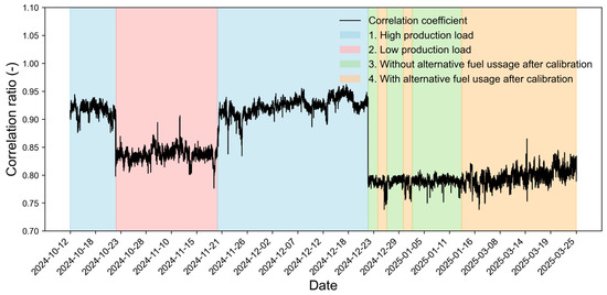
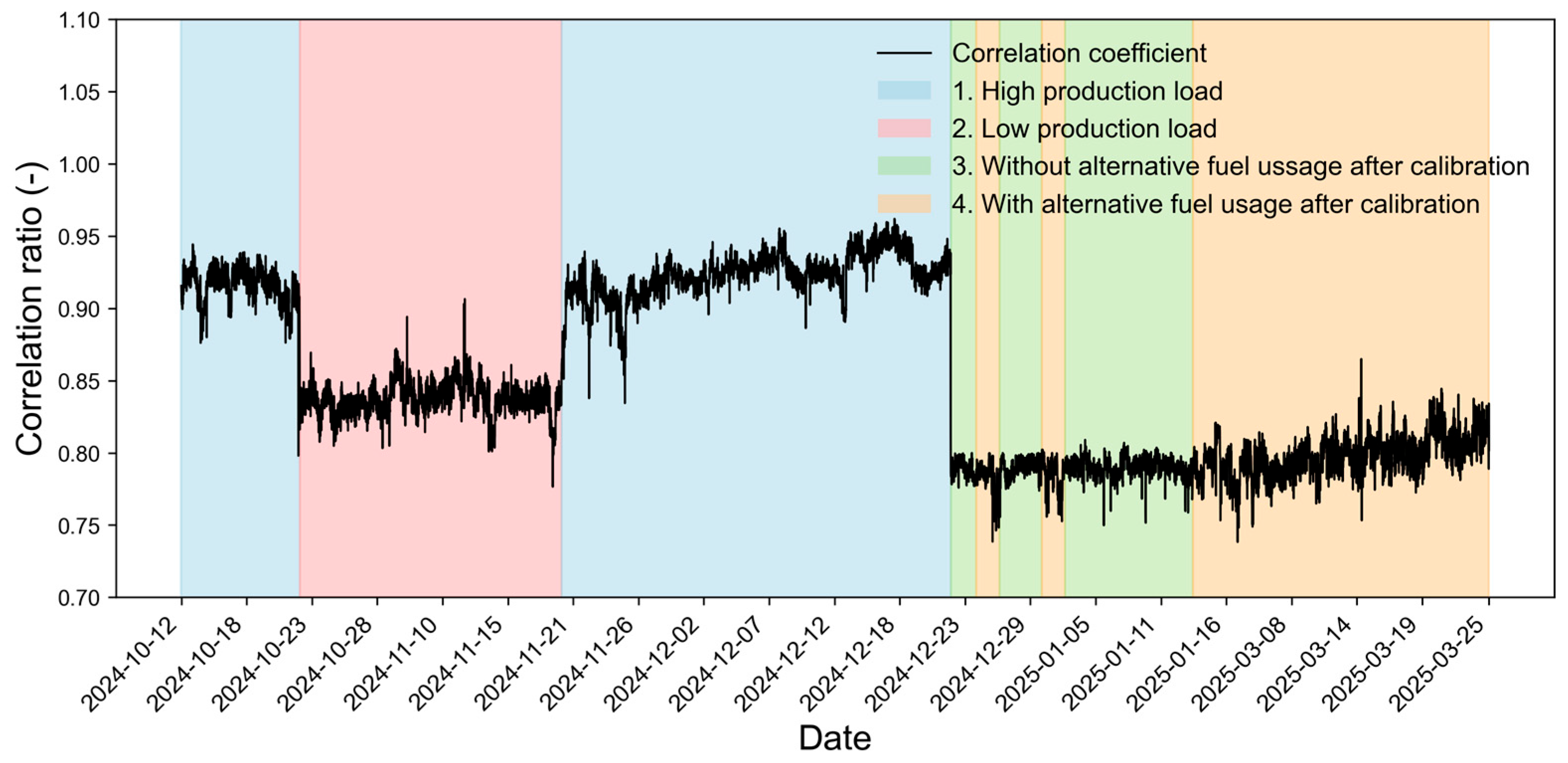
Combining the correlation coefficient analysis in Figure 3 with the operating status in Figure 7. Figure 8 illustrates the relationship between the correlation coefficient and the operating conditions. The first noticeable change in the correlation coefficient occurred from 22 October to 20 November, where a decrease in production load coincided with a drop in the correlation coefficient. The second notable change took place on 22 December. The calibration of the flue gas humidity meter caused the recorded humidity to drop from about 27% to 14%, which instantly increased the CEMS carbon emissions by about 18%, and then led to a sharp decrease in the correlation coefficients. From late December 2024 to 26 March 2025, the enterprise intermittently used waste textiles as an alternative fuel, which reduced coal consumption. Since certain components in the waste textiles can affect the quality of clinker, adjustments to the production process were made. These adjustments may have impacted the relationship between the two carbon emission datasets. Metal slag was consistently used as an alternative raw material during the experiment period. The use of fluorite waste was only suspended from 26 November 2024 to the end of January 2025. Based on comparative analysis, fluorite usage showed no significant effect on the correlation coefficient.

Figure 8. Relationship between the correlation coefficients and operating status.

Given that the impact of alternative fuel on the correlation coefficient remained unclear, this study developed the following operating condition classifications to evaluate the stability of the relationship between the two types of monitoring data under different operating conditions. Among them, operating condition 5 combined operating conditions 3 and 4 for further analysis.

Operating condition 1: High-load operation stage;

Operating condition 2: Medium-load operation stage;

Operating condition 3: Operation stage without alternative fuel use after instrument calibration;

Operating condition 4: Operation stage with alternative fuel use after instrument calibration;

Operating condition 5: Operation stage after instrument calibration.

3.3. Correlation Model Construction

In this experiment, the mean correlation coefficient was adopted as the core adjustment basis, and the carbon emissions from CEMS were adjusted to align with the level of CBM, in order to eliminate the influence of systematic error on the consistency of carbon emissions between the two monitoring methods. When the carbon emissions from the adjusted CEMS and CBM showed good consistency and the total relative error remained within a narrow range, the correlation model was considered to be successfully constructed, indicating a stable correlation between CBM and CEMS.

3.3.1. Mean Value of Correlation Coefficients

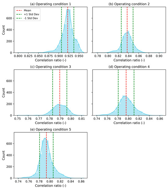
This study assumed an approximately linear proportional relationship between CBM and CEMS emissions across operating conditions. From a physical perspective, both CBM and CEMS emissions were primarily driven by production intensity within a given operating condition. Although the two monitoring approaches were subject to different sources of uncertainty and short-term fluctuations, their emission estimates were expected to respond in a similar manner to changes in production. This assumption was further supported by the statistical characteristics of the ratio between CBM and CEMS emissions. As shown in Figure 9, the emission ratios exhibit a unimodal and approximately symmetric distribution. This was consistent with a stable linear mapping between CBM and CEMS emissions perturbed by relatively small random fluctuations. In a general linear formulation, $E_{CBM}=a+b{E}_{CEMS}$, where a is expected to be negligible relative to the emission magnitude in this study. This is because, in the absence of production, both CBM and CEMS emissions theoretically approach zero. Therefore, within each operating condition, CBM and CEMS emissions can be approximated as linearly proportional.

Figure 9. Distribution of correlation coefficients under Different operating conditions.

Table 1 presents the statistical results for the mean and standard deviation of the correlation coefficients under different operating conditions. From the perspective of mean values, the correlation coefficients varied among operating conditions. Dip Test results for the correlation coefficients in five individual operating conditions are shown in Figure 9, with produced p-values ranging from 0.88 to 0.99, confirming unimodality for operating conditions 1–5. Among them, the mean correlation coefficient for operating condition 1 was the highest, reaching 0.922, indicating the smallest difference between the carbon emissions obtained by CEMS and CBM under this operating condition and relatively strong consistency between the two types of monitoring datasets. Following that, operating condition 2 had a mean correlation coefficient of 0.838. The mean values of operating conditions 3, 4, and 5 were similar, suggesting that the carbon emission correlations between the two monitoring methods were relatively close in these conditions. Since these operating conditions were classified based on alternative fuel usage, these results implied that alternative fuel usage did not significantly affect the distribution of the correlation coefficients. At the same time, the standard deviations across the five operating conditions differed minimally, ranging from 0.011 to 0.015, indicating that the dispersion of the correlation coefficients within each operating condition was nearly identical.

Table 1. Statistical description of correlation coefficients.

Operating Condition	Mean	Standard Deviation
1	0.922	0.0112
2	0.838	0.0115
3	0.789	0.0067
4	0.796	0.0150
5	0.793	0.0130

3.3.2. Correlation Model Test

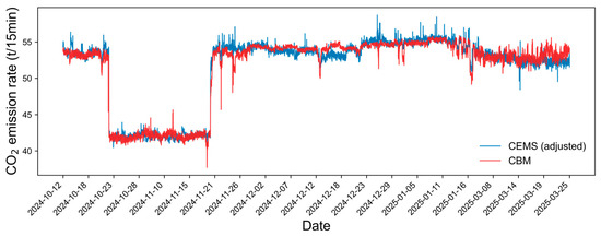
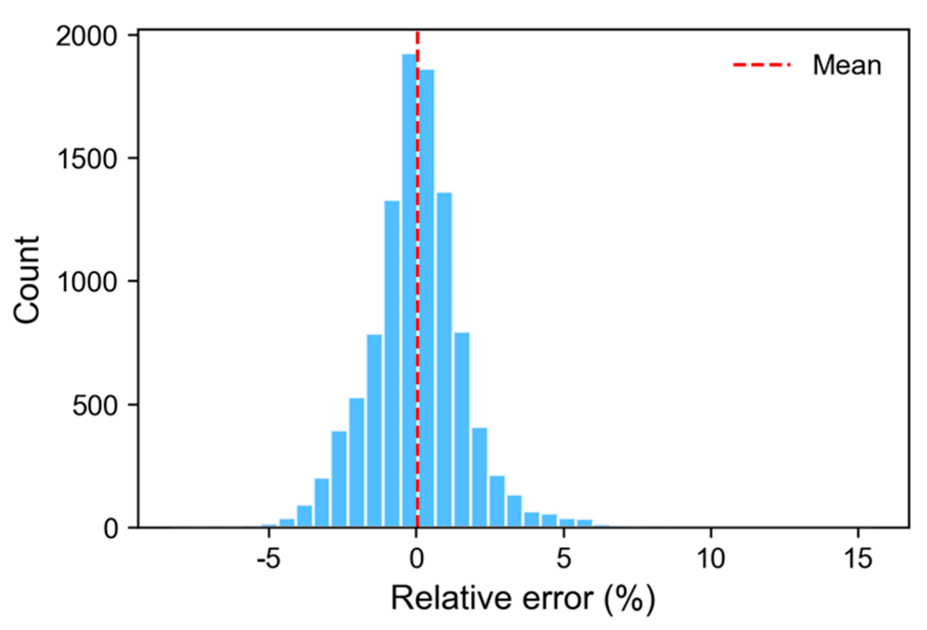
In this study, the original CEMS-based carbon emissions were adjusted by multiplying them by the mean correlation coefficient of their respective operating condition. Figure 10 shows the comparison of carbon emissions after adjustment for operating conditions 1, 2, and 5. The adjustment results for operating conditions 1, 2, 3, and 4 were highly similar. After the adjustment, the fit between the two types of carbon emission monitoring data was improved significantly, both in terms of overall levels and fluctuation ranges, with the peak and valley positions aligning closely. In addition, the systematic deviation caused by production load fluctuations, instrument calibration, and other factors were largely eliminated. The average relative error dropped to about 0.01%, and the error distribution shifted from a multi-peak distribution to an approximate normal distribution (Figure 11), indicating the successful establishment of the correlation model. The model can be further applied for missing value imputation and abnormal data identification for both types of monitoring datasets.

Figure 10. Comparison of CBM and adjusted CEMS emissions.

Figure 11. Relative error distribution between that of CBM and adjusted CEMS emissions.

3.4. Abnormal Data Diagnosis

In this experiment analysis, the reliability of the correlation model was studied by artificially perturbing the data. Table 2 shows the average detection rates of abnormal data under different levels of data manipulation. The detection rate was defined as the proportion of artificially manipulated samples that were correctly identified as abnormal, relative to the total number of manipulated (positive) samples. When the degree of artificial manipulation was 0 (i.e., no manipulation), the theoretical detection of failed tests should be 0. Any non-zero detection rates in this case indicated a nonzero false-positive rate in the mean value test. Such false-positive detection may arise from a relatively high overall standard deviation in the datasets or the presence of some inherent abnormal values. Notably, the false-positive rates for operating conditions 3 and 4 were relatively high.

Table 2. Detection rate of abnormal data across different operating conditions and manipulation degrees.

Artificial Manipulation Degree	Operating Condition 1	Operating Condition 2	Operating Condition 3	Operating Condition 4	Operating Condition 5
0	0	3%	10%	7%	3%
2%	93%	90%	100%	63%	93%
5%	100%	100%	100%	100%	100%
10%	100%	100%	100%	100%	100%
15%	100%	100%	100%	100%	100%

As the degree of artificial manipulation increased, the abnormal detection rate also increased. At a 2% artificial manipulation level, the detection rate for operating condition 4 was only 63%, which was significantly lower than that for the other operating conditions. The main reason was the large dispersion in the correlation coefficients for operating condition 4, which affected the accuracy of the statistical test. When artificial manipulation level reached 5% or higher, the detection rates across all operating conditions stabilized at 100%, indicating the model’s strong ability to identify medium- and high-level artificial manipulation.

The main purpose of classifying the operating conditions was to categorize the correlation coefficients into well-defined groups to enhance the efficiency of abnormal data diagnosis. Generally, dividing the experimental data into operating conditions 1, 2, and 5 resulted in higher identification efficiency for abnormal data than dividing it into operating conditions 1, 2, 3, and 4. The false-positive rates for operating conditions 1, 2, and 5 were all below 3%. An anomaly detection rate of 90% or higher could be achieved for data manipulation of 2% or above. Dividing the data into three operating conditions provided reliable technical support for controlling the risk of emission data manipulation. Furthermore, given the three-peak distribution of correlation coefficients, it was more reasonable to classify the operating conditions and the corresponding correlation coefficients into three groups: conditions 1, 2, and 5. Since the difference between operating conditions 3 and 4 was solely alternative fuel usage and operating condition 5 was the combination of conditions 3 and 4; it was not recommended to use alternative fuel utilization as the sole criterion for operating condition classification.

4. Conclusions

High-quality carbon emission data is an important prerequisite for the standardized operation of the carbon market. To enhance the emission data quality and mitigate data manipulation in cement enterprises, this study utilized high-frequency monitoring data from both CBM and CEMS. A systematic analysis was conducted on the correlation between the two datasets, leading to the development of a correlation model and the establishment of a statistically based abnormal data detection system. This study proposed a methodological framework in which, after appropriately classifying operating conditions for a case plant, the distribution of the ratio of CEMS to CBM emissions can be used to diagnose anomalous data. The proposed approach is transferable to other cement plants and similar industrial sectors with stable operational characteristics. The main conclusions are as follows:

First, the consistency between CBM and CEMS carbon emission data in cement enterprises was unsatisfactory, with point-to-point deviations ranging from 5% to 30%. Analysis of the ratio between the two datasets revealed that the correlation coefficients exhibited a multi-peak distribution. This indicated that the correlation coefficients were concentrated in multiple regions. Variations in production and operational parameters during the study were found to influence the magnitude of these coefficients.

Second, operating conditions were classified based on the analysis of the mean correlation coefficients and the results of abnormal data detection. The practical application required accurate classification of operating conditions tailored to each individual facility. In this study, the classification primarily reflected the fluctuations in production load and instrument calibration operations. Although alternative fuel usage influenced the correlation coefficients to some extent, it was not recommended to use as a primary criterion for classifying operating conditions.

Third, after adjusting CEMS emissions using the mean correlation coefficients under each operating condition, the total emission discrepancy between CBM and CEMS decreased from 17.87% to 0.01%, indicating higher data correlation. In cases where either CBM or CEMS data was artificially manipulated, abnormal deviations were observed to be detectable through statistical tests, suggesting the potential to identify anomalies.

Finally, a statistical mean test method was adopted to detect anomalies in artificially manipulated data. In the absence of fraud, the false-positive rate could remain below 3%. When the manipulation level reached 2%, the detection rate of abnormal data exceeded 90%. The detection rate reached 100% at manipulation levels of 5% or higher. The correlation model could be used for missing-data imputation in both monitoring datasets and serve as the basis for identifying anomalies related to carbon data fraud risks.

In summary, although both high-frequency CBM and CEMS monitoring data are subject to method-specific uncertainties from emission factors, LHV measurements, weighing systems, sensor drift, and flowmeters, this study demonstrated that, after operating conditions were properly classified and data are aligned, a high degree of correlation can be achieved between CBM and CEMS. It is also worth noting that an improved degree of correlation cannot reduce the cumulative uncertainty of either method, and therefore cannot eliminate any systematic data biases that may exist between two methods. Under such conditions, both false-positive and false-negative rates of abnormal data diagnosis remained low. This method not only makes it more difficult for enterprises to commit data fraud by increasing barriers to fraud but also has the potential to reduce regulatory costs through digital means and to provide reliable technical support for emission data quality control.

References

- Cheng, D.; Reiner, D.M.; Yang, F.; Cui, C.; Meng, J.; Shan, Y.; Liu, Y.; Tao, S.; Guan, D. Projecting future carbon emissions from cement production in developing countries. Nat. Commun. 2023, 14, 8213. [Google Scholar] [CrossRef] [Scilit] [PubMed]
- Liao, S.; Wang, D.; Xia, C.; Tang, J. China’s provincial process CO2 emissions from cement production during 1993–2019. Sci. Data 2022, 9, 165. [Google Scholar] [CrossRef] [Scilit] [PubMed]
- Liu, X.; Yang, L.; Du, J.; Zhang, H.; Hu, J.; Chen, A.; Lv, W. Carbon and air pollutant emissions forecast of China’s cement industry from 2021 to 2035. Resour. Conserv. Recycl. 2024, 204, 107498. [Google Scholar] [CrossRef] [Scilit]
- China Building Materials Academy Co., Ltd. A Study on the Carbon Neutrality Pathways of China’s Cement Industry; China Building Materials Academy Co., Ltd.: Beijing, China, 2023. [Google Scholar]
- State Council of the People’s Republic of China. China Expands Carbon Trading Market to Steel, Cement, Aluminum Smelting Sectors. 2025. Available online: https://english.www.gov.cn/news/202503/27/content_WS67e487ddc6d0868f4e8f1358.html (accessed on 27 March 2025).
- People’s Daily. The Provisional Regulations on the Administration of Carbon Emission Trading are Recently Announced, Making Targeted Provisions for Current Difficulties in the Carbon Market. Ministry of Ecology and Environment of the People’s Republic of China. 2024. Available online: https://www.mee.gov.cn/home/ztbd/2022/sthjpf/fgbzjd/202404/t20240418_1071069.shtml (accessed on 27 February 2024).
- Shi, B.; Li, N.; Gao, Q.; Li, G. Market incentives, carbon quota allocation and carbon emission reduction: Evidence from China’s carbon trading pilot policy. J. Environ. Manag. 2022, 319, 115650. [Google Scholar] [CrossRef] [Scilit] [PubMed]
- Xu, H.; Yang, R. Does carbon market improve ESG performance? Evidence from China. J. Clean. Prod. 2025, 514, 145810. [Google Scholar] [CrossRef] [Scilit]
- Song, Y.; Luo, X.; Lu, Y.; Qian, J.; Zhang, W.; Liu, L.; Huang, J.; Zhao, X.; Zhang, D. Improving the data quality of CO2 continuous emissions monitoring systems: In the context of China’s emissions trading scheme. Environ. Impact Assess. Rev. 2025, 115, 108037. [Google Scholar] [CrossRef] [Scilit]
- Zeng, Y.; Faure, M.G.; Feng, S. Localization vs globalization of carbon emissions trading system (ETS) rules: How will China’s national ETS rules evolve? Clim. Policy 2025, 25, 996–1010. [Google Scholar] [CrossRef] [Scilit]
- Chen, M. A Preliminary Study on the Path to Improving Carbon Emission Data Quality in the Electric Power Industry. China Sci. Technol. J. Database Ind. A 2022, 10, 42–45. [Google Scholar]
- Liesen, A.; Hoepner, A.G.; Patten, D.M.; Figge, F. Does stakeholder pressure influence corporate GHG emissions reporting? Empirical evidence from Europe. Account. Audit. Account. J. 2015, 28, 1047–1074. [Google Scholar] [CrossRef] [Scilit]
- Ministry of Ecology and Environment of the People’s Republic of China. Notice on Issuing the Guidelines for Accounting and Reporting of Greenhouse Gas Emissions for Enterprises–Cement Industry (CETS-AG-02.01-V01-2024) and Three Other National Technical Specifications for the Carbon Emissions Trading Market. 2024. Available online: https://www.mee.gov.cn/xxgk2018/xxgk/xxgk06/202409/t20240914_1086067.html (accessed on 14 September 2024).
- Majanne, Y.; Korpela, T.; Uotila, T. EU Emission Trading Related CO2 Monitoring in Power Plants. IFAC Proc. Vol. 2014, 47, 1361–1366. [Google Scholar] [CrossRef] [Scilit]
- Eggleston, H.S.; Buendia, L.; Miwa, K.; Ngara, T.; Tanabe, K. 2006 IPCC Guidelines for National Greenhouse Gas Inventories; Institute for Global Environmental Strategies (IGES): Hayama, Japan, 2006. [Google Scholar]
- Xiong, L.; Wang, M.; Mao, J.; Huang, B. A Review of Building Carbon Emission Accounting Methods under Low-Carbon Building Background. Buildings 2024, 14, 777. [Google Scholar] [CrossRef] [Scilit]
- Yan, H.-S.; Tan, X.-C.; Zeng, A.; Kong, L.-S. China’s carbon accounting system in the context of carbon neutrality: Current situation, challenges and suggestions. Adv. Clim. Change Res. 2023, 14, 23–31. [Google Scholar] [CrossRef] [Scilit]
- Department of Resource Conservation and Environmental Protection, NDRC. Notice on Further Strengthening the Action Plan for the Construction of a Standard Metrology System for Carbon Peaking and Carbon Neutrality (2024–2025). 2024. Available online: https://www.ndrc.gov.cn/xwdt/tzgg/202408/t20240808_1392292.html (accessed on 8 August 2024).
- China-Europe Association for Technical and Economic Cooperation. China Plans to Strengthen Its Carbon Emissions Statistical Accounting System. Climate Cooperation. 2024. Available online: https://climatecooperation.cn/climate/china-plans-to-strengthen-its-carbon-emissions-statistical-accounting-system/ (accessed on 27 June 2024).
- Srivastava, R.P.; Kumar, S.; Tiwari, A. Continuous emission monitoring systems (CEMS) in India: Performance evaluation, policy gaps and financial implications for effective air pollution control. J. Environ. Manag. 2024, 359, 120584. [Google Scholar] [CrossRef] [Scilit] [PubMed]
- Teh, H.Y.; Kempa-Liehr, A.W.; Wang, K.I.-K. Sensor data quality: A systematic review. J. Big Data 2020, 7, 11. [Google Scholar] [CrossRef] [Scilit]
- Ministry of Ecology and Environment of the People’s Republic of China. Response to Proposal No. 5442 of the Second Session of the 14th National People’s Congress. 2024. Available online: https://www.mee.gov.cn/xxgk2018/xxgk/xxgk13/202412/t20241204_1098022.html (accessed on 27 August 2024).
- Wei, Z. Tackling Carbon Monitoring: Bottlenecks and Breakthroughs in CO2 Monitoring Technology for Thermal Power Plants. 2025. Available online: https://m.bjx.com.cn/mnews/20250529/1443967.shtml (accessed on 29 May 2025).
- Wang, X.; Liu, R.; Zhao, X. Cement enters the carbon market; Improving the reliability of emission data. China Cem. 2024, 7, 71–72. [Google Scholar]
- Ackerman, K.V.; Sundquist, E.T. Comparison of Two U.S. Power-Plant Carbon Dioxide Emissions Data Sets. Environ. Sci. Technol. 2008, 42, 5688–5693. [Google Scholar] [CrossRef] [Scilit] [PubMed]
- Quick, J.C. Carbon dioxide emission tallies for 210 U.S. coal-fired power plants: A comparison of two accounting methods. J. Air Waste Manag. Assoc. 2014, 64, 73–79. [Google Scholar] [CrossRef] [Scilit] [PubMed]
- Lee, S.; Choi, Y.; Woo, J.; Kang, W.; Jung, J. Estimating and comparing greenhouse gas emissions with their uncertainties using different methods: A case study for an energy supply utility. J. Air Waste Manag. Assoc. 2014, 64, 1164–1173. [Google Scholar] [CrossRef] [Scilit]
- Wang, X.; Xu, L.; Zhang, Q.; Zhang, D.; Zhang, X. Evaluating the data quality of continuous emissions monitoring systems in China. J. Environ. Manag. 2022, 314, 115081. [Google Scholar] [CrossRef] [Scilit] [PubMed]
- DL/T 2376-2021; Technical Specification for Continuous Emission Monitoring of Carbon Dioxide in Flue Gas from Thermal Power Plants. National Energy Administration: Beijing, China, 2021.
- GB/T 16157-2018; Technical Requirements and Test Procedures for Continuous Emissions Monitoring of SO2, NOX, and Particulate Matter in the Flue Gas Emitted from Stationary Sources. State Administration for Market Regulation: Beijing, China, 2018.
- T/BJEA 0002-2023; Technical Specification for Quantification and Verification of Greenhouse Gas Emission Reduction of Carbon Capture, Utilization and Storage (CCUS) Project. CN-TUANTI: Beijing, China, 2023.
- GB/T 32151.8-2023; Carbon Emission Accounting and Reporting Requirements—Part 8: Cement Manufacturing Enterprises. State Administration for Market Regulation: Beijing, China, 2023.
- Alemayehu, F.; Sahu, O. Minimization of Variation in Clinker Quality. Adv. Mater. 2013, 2, 23–28. [Google Scholar] [CrossRef] [Scilit]
- Beijing Municipal Ecology and Environment Bureau. Announcement of the Beijing Municipal Ecology and Environment Bureau on the Quality Assessment of the Verification Work of the Beijing Carbon Market in 2025. 2025. Available online: https://sthjj.beijing.gov.cn/bjhrb/index/xxgk69/zfxxgk43/fdzdgknr2/325924085/743890520/index.html (accessed on 16 January 2026).
- DB44/T 2596-2024; Technical Requirements for Continous Emission Monitoring of CO2 from Thermal Power Plant. Guangdong Provincial Market Supervision and Administration Bureau: Guangzhou, China, 2024.
- Casella, G.; Berger, R. Statistical Inference; Chapman and Hall/CRC: New York, NY, USA, 2024. [Google Scholar] [CrossRef] [Scilit]
- HJ 75-2017; Specifications for Continuous Emissions Monitoring of SO2, NOx, and Particulate Matter from Stationary Sources. China Environmental Science Press: Beijing, China, 2017.
Disclaimer/Publisher’s Note: The statements, opinions and data contained in all publications are solely those of the individual author(s) and contributor(s) and not of MDPI and/or the editor(s). MDPI and/or the editor(s) disclaim responsibility for any injury to people or property resulting from any ideas, methods, instructions or products referred to in the content. |
© 2026 by the authors. Licensee MDPI, Basel, Switzerland. This article is an open access article distributed under the terms and conditions of the Creative Commons Attribution (CC BY) license.