


Abstract
In grids with limited transformer and transmission–distribution capacity, the licensed power of solar plants is defined on the AC side, and capacity overshoot is not permitted. Since photovoltaic (PV) panels rarely reach standard test conditions, a DC/AC ratio above 1.0 with inverter power limitation can use licensed capacity more efficiently, though increasing ratios bring clipping losses. In this study, the optimum DC/AC ratio was determined financially for a photovoltaic power plant (PVPP) in Niğde/Edikli with 15.237 MWp installed DC and 10 MWe licensed power. Simulated with PVSOL at a 1 min time step and compared month by month with SCADA data, the model reproduces the annual energy delivered to the grid of 2021 to a relative deviation of −2.66% and the performance ratio to −1.93%; the comparison is reported as a long-term yield consistency check, since the simulation is driven by a climate dataset covering 2001–2020 while the measurement covers a single year. Unlike the generalized kWp-based cost approach in the literature, 25 scenarios (10–16 MWp; DC/AC 1.0–1.6) were examined using an item-based cost model separating costs affected and unaffected by installed power. Raising installed power from 10 to 16 MWp increased grid-delivered energy by ~41.9%, while clipping loss rose from less than 0.01% to 13.38%. At a real discount rate of 8% and over a 25-year assessment period, the discounted payback period (9.42 years), the internal rate of return (12.32%) and the levelized cost of energy (0.0823 USD/kWh) reach their best values jointly at 12.75–13.00 MWp (DC/AC 1.275–1.30). Because the three indicators vary only slightly between neighboring configurations, the result is reported as the economically viable range of 12.00–14.00 MWp (DC/AC 1.20–1.40), within which all three remain within 0.9% of their best values. The position of this range is conditional on the item-based cost-scaling rule: the constant-cost-per-kWp model places the ratio-based optimum at 10.50–11.00 MWp, and fixing half or all of the four site items places it at 13.50–14.00 and 14.50–15.25 MWp. The net present value at the same discount rate reaches its maximum of USD 4,429,253 at 14.25 MWp and therefore favors the upper part of that range.
1. Introduction
1.1. Background and Motivation
World energy demand is continuously rising with population and economic growth, while fossil fuels still dominate global electricity and heat generation [1]. The excessive use of fossil fuels increases greenhouse gas emissions and pollution, while the depletion of oil and natural gas reserves and the rise in energy costs create economic problems in countries that do not possess these resources; in the case of Türkiye, this takes the form of a heavy reliance on imported natural gas, which threatens energy independence and increases the current account deficit [1]. Because they are environmentally friendly, reduce external dependence, and support the use of domestic energy, renewable energy sources offer a significant alternative to these problems; solar energy stands out as a clean option with flexible installation and low maintenance costs. PV systems, whose costs have fallen with technological advances, are also becoming widespread in this direction [2].
From the investor’s perspective, a feasibility study must absolutely be carried out before a decision on capital allocation is made. Simulation tools such as PVsyst, PVSOL, PVGIS, and Retscreen are the analytical resources used in this process [3]; however, since software calculations may not be entirely realistic, it is essential that the simulation results be tested against actual production values and that the climate data used provide the closest possible match with the region in which the installation will be carried out.
In many countries, including Türkiye, various legal regulations exist for grid-scale commercial licensed power plants on grounds of grid reliability, fair competition, financial stability, and security of energy supply. One of these concerns the licensed power capacity: the licensed power refers to the alternating current power at the grid connection point and is audited; although the direct current power capacity is determined within the scope of project design, the licensed capacity is defined on the basis of AC power. In Türkiye, capacity overshoot in licensed power plants is not permitted except under special circumstances, and overshoot is regarded as a serious violation that may result in an administrative fine and revocation of the license [4]. Therefore, capacity planning must be carried out carefully at the project stage.
Because the standard test conditions under which panels are tested rarely occur during the year, PV power plants mostly produce below their DC power capacity; this means that the licensed AC power capacity cannot be utilized sufficiently [5,6]. The problem can be solved by designing the DC power capacity at a certain ratio above the licensed AC capacity and, where necessary, applying power limitation at the inverter. This ratio is the DC/AC ratio, which expresses the ratio of the total DC power of the panels to the AC output power of the inverter, and it is a decisive parameter in system design; for example, in a plant with a licensed capacity of 10 MWe, the total DC power of the panels may be 12 MWp (DC/AC ratio = 1.2). Inverters have traditionally been dimensioned at a ratio of about 1.2, and the ratio is shifting upwards because clipping part of the DC power in hours of high irradiance is worthwhile, so that the cost-optimal ratio can be as high as 1.7 for certain locations [7].
In small or medium-scale systems where the licensed power is not defined on the AC side, selecting this ratio above 1.0 offers two additional advantages: reducing initial investment costs by downsizing the inverter capacity, and operating the inverter at higher efficiency under low-irradiance conditions [8]. Downsizing the inverter capacity reduces not only the inverter cost but also the transformer power, cable cross-section, and the dimensions of the connection equipment, thereby lowering system installation costs [9]. Since inverter efficiency decreases rapidly at low power values, the optimum ratio lies in the 1.1–1.2 range for high-efficiency inverters, while it rises to the 1.3–1.4 band in low-irradiance regions [10]. However, the return from oversizing is not unlimited; increasing the ratio improves the project economics only up to a certain point, beyond which energy losses and additional costs exceed the benefit obtained from the additional panels [11]. In addition, sizing the array above the nominal power of the inverter may have a negative effect on inverter lifetime due to increased internal heating [12,13].
The focus of this study differs from the free design regime defined above: in the plant considered, the installed DC power (15.237 MWp) is above the licensed power (10 MWe) and corresponds to a value of 1.5237 in terms of the DC/AC ratio. Therefore, power limitation here is not a by-product of an economic sizing preference, but a constraint arising from the licensed power that must be applied during operation. This distinction determines both the formulation of the optimization problem and the economic interpretation of the results. Without envisaging energy storage, the study aims to determine the DC power capacity that will provide the highest economic benefit from the licensed AC power capacity through the application of power limitation and in accordance with the climatic conditions of the region in which the plant is installed.
At a DC/AC ratio of 1.0 the clipping loss is not zero but negligible: the array is rated at standard test conditions while the power available at the inverter input varies at every simulation step, so the AC limit is exceeded in some intervals and a small amount of energy is clipped—470.91 kWh per year, or 0.0028% of the energy delivered to the grid, in the 10 MWp configuration analysed in Section 6. The principal disadvantage of this ratio is therefore not the clipping loss but the fact that the AC capacity of the inverter cannot be fully utilized [14]. Raising the ratio above 1.0 gives rise to a flattening effect in the daily production profile due to power limitation and to the associated clipping losses; under these conditions, in which the inverter reaches its maximum power, the daily energy production curve takes on a “flat-topped” form [15]. Figure 1 shows the power–time graphs for days on which a PV array, by being oversized, reaches and does not reach the nominal AC power capacity of the inverter. Although power limitation in inverters may appear unusual, it is a standard industry practice; in installations with high DC power capacity that are made without energy storage, a portion of the energy produced cannot be transferred to the grid, and this means that the investment aimed at capacity expansion remains idle. Therefore, determining the DC/AC ratio in accordance with the climatic conditions of the region in which the installation is carried out is an important optimization problem; in both of the extreme cases defined, economic losses occur and the payback period of the investment is extended.
Figure 1.
Energy production graphs in a PV plant with inverter limitation: (a) A day with power limitation. (b) A day without power limitation.
In the financial analysis of PV systems, costs are mostly calculated using a unit-cost-per-installed-power approach, generally based on amounts per kilowatt peak (kWp) or watt peak [2]. Although this method offers a practical and rapid approach for preliminary feasibility, it cannot adequately reflect variables dependent on site conditions such as mounting infrastructure, differences in support structures, cabling distances, ground and roof conditions, labor requirements, grid connection arrangements, and permitting and engineering expenses. This leads to a deviation of financial analysis results from implementation realities and to a reduction in the accuracy of key indicators such as the payback period, net present value (NPV), and internal rate of return (IRR) [16]. Therefore, instead of relying solely on the unit-cost-per-power approach in economic assessments, more comprehensive cost models that include site conditions and project-based uncertainties should be used.
In the literature reviewed, clipping has been addressed predominantly as a by-product of economically justified oversizing [17] or as a consequence of regulations that impose an upper limit on the ratio in order to smooth grid integration and increase the hosting capacity of the grid; it has been emphasized that the optimum ratio should be defined not by a single universal value but according to project-specific conditions [18]. However, a framework in which power limitation is treated not as a design-related side effect but as a legal operating constraint, and in which simulation accuracy and the optimum ratio are evaluated together under this constraint, remains lacking. In this study, a licensed PVPP located in the Edikli district of Niğde, in the Central Anatolia Region of Türkiye, with an installed panel power of 15.237 MWp and a licensed capacity limited to 10 MWe, is considered. The first objective of the study is to demonstrate the success of the PVSOL premium 2026 (R3) software in predicting the energy production data of a large-scale PV plant with power limitation applied, under the climatic conditions of the Central Anatolia Region specific to Niğde. The second objective is to economically analyze the application of power limitation in such licensed PV plants, in which the installed panel power is greater than the permitted licensed power. Accordingly, first a detailed modeling and simulation study was carried out using PVSOL, and the accuracy of the model was evaluated by comparing the data obtained with actual data in terms of energy production and economics. Subsequently, without changing the technical characteristics of the plant, 25 different PVSOL analyses were carried out by varying the installed power within the range of 10–16 MWp, and the optimum DC/AC ratio that would provide the highest economic benefit from the permitted 10 MWe licensed power was determined.
1.2. Related Works and Contributions
In the literature, the concept of the DC/AC ratio is also referred to by names such as Inverter Loading Ratio (ILR), Inverter Sizing Ratio, Inverter Sizing Factor, Inverter Power Ratio, Optimum Sizing Ratio and Sizing Ratio, and there is no complete unity in the terminology [13,15,19,20,21,22].
The upper limit of oversizing permitted by inverter manufacturers varies considerably by brand and model; for SolarMax this limit is 15%, whereas the recommended range for ABB is limited to 0.80–0.90, while some manufacturers permit much higher ratios such as 130% and 200% [15,23].
The decline in module costs has made oversizing the array power relative to the inverter a common design practice [18]; Silva et al. list the objectives of this approach as a higher capacity factor, increased energy yield and a reduced cost of generation [17]. Pandey et al., on the other hand, emphasize that clipping loss arises at high DC/AC ratios, yet a high ratio provides an advantage under low-irradiance conditions, and therefore completely preventing clipping would not be a correct decision [24]. Medojevic et al. show that clipping is not constant throughout the day and is concentrated only in the hours when the sun is high and on clear days [25].
Various studies on the oversizing of inverters report that the optimum inverter sizing ratio is approximately 1.2 and that it may vary within the range of 1.1–1.4 depending on climate, irradiance, orientation/tilt, mounting position and inverter type [15,26,27,28]. İşin and Çetinkaya state that the 1.25–1.4 band of the DC/AC ratio is more advantageous from the investor’s perspective [14]. Medojevic et al., in turn, show that in high-irradiance regions clipping begins at a ratio of approximately 1.25, whereas in cloudy climates and under unfavorable orientations this threshold rises to around 1.35 [25].
The determining role of geographical location stands out through mutually supporting findings. Beyoğlu and Demirtaş compared two arrays of the same capacity but with different orientations in Balıkesir/Türkiye; they calculated the optimum DC/AC ratios as 1.28 and 1.35, respectively, and the efficiencies as 91.55% and 90.62% [9]. Hazim et al. emphasize that the sizing ratio depends on geographical latitude and must be determined site-specifically due to different irradiance distributions and operating temperatures [15]. Deschamps and Rüther, in their study conducted in Brazil, calculated the optimum ILR as 1.26 for conventional crystalline silicon technology; when the same 0.5% overload loss criterion was applied, values of 1.15 for Bahia (latitude −12.4) and 1.20 for Florianópolis (latitude −27.6) were obtained, and they showed that this difference stems from the variation in irradiance levels between the regions [27]. Rodrigo et al. demonstrated that in the low-latitude semi-desert climate of Mexico, inverter clipping is the main factor limiting the annual DC/AC conversion efficiency [29].
Different results are also reported in the context of scale and location. Kaewnukultorn et al. state that for three different locations in the USA the lowest levelized cost of energy (LCOE) remains within the 1.1–1.4 DC/AC range, and that this wide range indicates that the ratio does not have a strong effect on LCOE [18]. In the analysis carried out by Díaz-Bello et al. on a 4.2 kWp system in Spain over the range of 0.9–2.1, the optimum ratios were found to be 1.63–1.87, and these configurations produced payback periods of 8–9 years; moreover, it was shown that azimuth and tilt angles markedly affect clipping losses [30]. In the optimization performed with a non-linear least-cost model for the Ukrainian electricity system, the DC/AC ratio was calculated as 1.59, and this configuration was found to reduce the LCOE by 4.2% compared with a ratio of 1.2 [31].
The study conducted by Kaewnukultorn et al. on battery-supported bifacial systems demonstrates that different financial indicators point to different DC/AC ratios: the fastest payback period highlights the 1.0–1.05 range, the highest NPV the 1.1–1.3 range, and the lowest LCOE the 1.1–1.4 range; it is stated that each indicator reflects a different value of the system [18]. The same research group shows that the highest NPV is strongly dependent on location; in Phoenix, where irradiance is high, the optimum ratio can rise to as high as 1.45, because the clipped energy can be stored in the DC-coupled battery [18]. The researchers explicitly emphasize that the system with the highest NPV is not always the system with the lowest LCOE [32]. Attention is also drawn to the technical limit of excessively high ratios; the annual energy production of a system with a DC/AC ratio of 1.7 remains comparable to that of a system with a ratio of 1.5, because the overgeneration raises the inverter operating voltage and the MPPT lowers the voltage, thereby reducing the DC output [32]. Zipp, on the other hand, reports that the selection of the ratio should be evaluated along the axis of financial efficiency, and that falling module prices and new time-of-use tariffs improve the economics of oversizing [11].
Balfour et al. show that clipping distorts the interpretation of the performance ratio, creating a masking effect in which, when the DC/AC ratio exceeds 1, the measured PR appears higher than the plant’s actual DC-side performance. The study proposes a continuous distribution function based solely on three basic factors for calculating the clipped energy and demonstrates that this yields more accurate results than hourly simulations. In the same study, for a system with a capacity of 1200 kW DC/900 kW AC, the annual clipping loss was calculated as 21,593 kWh with the analytical approach, 19,333 kWh with a 1 min simulation and 1929 kWh with an hourly simulation [12]. Pandey et al. also report that clipping loss can reduce the PR and that the method they propose can calculate the clipping loss with an accuracy of ±2% and a 95% confidence interval [24].
Bahloul et al., in the example of the 7.2 MW Kelmoney plant in Ireland, sized utility-scale energy storage systems with a statistical model to minimize clipping losses; they showed that with current cost data no storage technology is economically viable, but that under 2030 cost projections and an installation raised to ILR = 2, the NCA, NMC and LFP technologies could become viable; in this case, a 1 MW/4 h configuration was found to be the most suitable solution for LFP. The researchers state that the low number of annual clipping cycles limits storage revenue and that this application should be evaluated not on its own but together with additional grid services [33]. Müller et al., on the other hand, adopted a 1 min sampling interval for storage sizing under clipping losses in grid-connected plants; they present as justification that the PV plant output power exhibits low-pass filter behavior (equivalent cut-off frequency of 0.01 Hz) and that grid codes regulate power fluctuation on a minute basis [34]. Yao and Cai propose, for large-scale PV plants, a two-layer decision architecture that takes NPV, payback period and IRR as the outer objective function and storage capacity as the variable [35].
In their review, Kaewnukultorn et al. report that Umar et al., comparing ten PV simulation software packages, identified SAM, HOMER and PVsyst as the most common and effective tools, and that SAM can produce the annual performance ratio very close to actual measured values. In the same review, it is stated that Mondol et al. optimized the DC/AC ratio with a TRNSYS-based simulation in order to minimize the LCOE at certain locations in Europe [18]. Alsadi and Khatib classified the criteria, constraints, models, techniques and software tools used in PV system sizing, and stated that numerical approaches are the most widely used but, due to methodological differences, the most difficult to compare [3]. Hazim et al., in turn, propose a deep learning-based approach for automatically calculating the DC/AC ratio under variable climatic conditions [15].
Temporal resolution lies at the center of the methodological discussion. Balfour et al. show that hourly simulations underestimate clipping losses, and that the analytical approach based on the continuous distribution function, with its clipping estimate of 21,593 kWh, is the closest to reality compared with the values of 19,333 kWh for the 1 min simulation and 1929 kWh for the hourly simulation. The authors state that clipping can occur even at time scales below 1 min and that 1 min data are the highest resolution available for comparison [12]. Müller et al. also adopted a 1 min sampling interval in the calculation of the clipped energy [34].
Thom et al., analyzing selected variants of a large-scale plant in Poland, reported LCOE values within the range of 0.10–0.13 EUR/kWh and stated that larger plants generally show higher profitability, but that there is no strict linear relationship between capacity and profitability. The authors note that the results overlap with the findings for the Baltic countries (0.08–0.09 EUR/kWh) and Hungary (7–9 years payback) and emphasize the dominant effect of CAPEX on the economic results [1].
When the above studies are considered together, three gaps come to the fore. First, findings regarding the optimum DC/AC ratio focus predominantly on residential or small-scale systems and on the general grid scale; ratio determination based on financial analysis specifically for commercial plants whose AC side is fixed by license remains limited. Second, the unit-cost-per-power approach is common in economic assessments, while cost models based on item-by-item actual price data at the MW scale are rare. Third, studies in which technical, economic, and environmental dimensions are addressed in an integrated manner are limited. This study addresses the aforementioned gaps in the case of an MW-scale plant whose AC side is limited by license. What the framework contributes to the current techno-economic sizing studies follows from these gaps. In the literature, DC oversizing under an AC limit is treated as a free design choice whose economics are evaluated with costs expressed per kWp; in a licensed plant, the DC capacity above the AC rating is the condition under which the plant operates, and the items that the export limit keeps independent of the DC capacity—the license fee, the transmission line, the inverter, the transformer, the switchgear and the remaining AC-side equipment, 32.1% of the CAPEX of the as-built plant—are precisely the items that the unit-cost approach cannot separate. The framework therefore treats the export limit as a constraint of the optimization and the cost model as part of the result, and the comparison reported in Section 5 quantifies what this changes: calibrated to agree at the as-built plant, the item-based and the constant-cost-per-kWp models place the optimum at 12.75–13.00 MWp (DC/AC 1.275–1.30) and at 10.50–11.00 MWp (DC/AC 1.05–1.10), respectively. The cost-scaling rule, and not the price level, therefore determines the position of the optimum, and a study of a licensed plant that adopts the conventional unit-cost approach will understate the DC capacity that the license makes economic. The following items summarize the original contributions of the study relative to its position in the literature.
- Item-based real cost model: Instead of the cost-per-Wp/kWp approach common in the literature, a detailed cost model was established on the basis of the actual prices of all material and service items used in the plant, and the items were classified according to their dependence on installed power. This classification reveals that the items dependent on the installed DC capacity account for 67.7% of the total investment and the items dependent on the AC capacity for 32.1%, while the items independent of both account for only 0.18%; because the AC side of the plant is fixed by the license, the items in the latter two groups do not vary with the installed DC power.
- Criticality of cost accuracy at the MW scale: In a plant where the licensed power is defined on the AC side and the installed DC power is significantly above this limit, the share of site-dependent cost items grows, so the risk of deviation in the unit-power approach increases and an item-based model becomes mandatory.
- Framing of clipping as a legal operating constraint: Clipping is treated not as a design-related side effect, but as a legal operating constraint aimed at ensuring the most efficient use of AC capacity in this structure, in which the licensed capacity is defined on the AC side.
- Validation of the simulation with real operating data: The plant was modeled at a 1 min time step and the simulated results were compared month by month with supervisory control and data acquisition data, the model reproducing the measured annual energy generation to a relative deviation of −2.66% and the measured performance ratio to −1.93%. Considering the necessity of high temporal resolution for the accurate estimation of clipping losses [36], this modeling validated at the MW scale offers an original contribution.
- Integrated technical–economic–environmental assessment: 25 scenarios with DC/AC ratios varying in the range of 1.0–1.6 were analyzed together with their technical, economic, and environmental dimensions; it was concretely demonstrated that the range indicated by technical performance indicators and the value indicated by economic indicators may differ. The environmental dimension was included in the assessment through the annual avoided CO2 emission indicator.
- Geographical location-based regional finding: Since it is known that the sizing ratio depends on site characteristics such as local irradiance distribution and geographical latitude, the band of 1.275–1.30 determined specifically for Niğde/Edikli can be regarded as a regional contribution that confirms the “optimal according to circumstances” approach.
The remaining sections of the article are organized as follows. Section 2 addresses Türkiye’s solar energy potential and the legislation on licensed electricity generation. Section 3 introduces the general and technical characteristics of the Edikli PVPP together with the location and climate data of the site. Section 4 presents the modeling of the plant with the PVSOL software and the simulation results obtained; these results are compared with the actual energy production data obtained through the SCADA system. Section 5 introduces the item-based cost model and calculates the CAPEX values for 25 different installed power scenarios with DC/AC ratios varying in the range of 1.0–1.6. Section 6 compares the techno-economic results of these scenarios and determines the optimum DC/AC ratio.
2. Türkiye’s Solar Energy Potential and Licensed Electricity Generation Legislation
2.1. Türkiye’s Solar Energy Potential
Türkiye has a pronounced solar energy potential owing to its geographical location. According to the Türkiye Solar Energy Potential Atlas (GEPA) compiled by the Ministry of Energy and Natural Resources, the annual average sunshine duration is 2741 h and the average annual total irradiation 1527.46 kWh/m2 [37]. The general potential outlook and the monthly average global radiation distribution of the Atlas are presented in Figure 2.
Figure 2.
Solar radiation general potential outlook of Türkiye [38].
2.2. Licensed Electricity Generation Legislation
The basic framework regulation of the Turkish electricity market is Electricity Market Law No. 6446 dated 14 March 2013, which repealed Law No. 4628 and restructured the market on the basis of bilateral contracts and the balancing mechanism. Generation, transmission, distribution, wholesale and retail sale and autoproducer activities are all subject to licensing, and the legal entities authorized to obtain a license include public and private sector generation companies and organized industrial zone legal entities [39].
Legal entities wishing to operate in the market must first obtain a pre-license from the Energy Market Regulatory Authority; the pre-license period, determined by Board decision, does not exceed 36 months excluding force majeure cases, and the investor must obtain the permits, approvals and similar documents arising from the legislation within it. Obtaining a generation license is then mandatory in order to proceed to the construction phase, and the license is granted for a minimum of 10 and a maximum of 49 years, taking into account the nature of the activity. EPDK obtains the opinions of the Turkish Electricity Transmission Corporation and the relevant distribution license holders on grid connection and grid use within 45 days [40].
Licensed legal entities may offer the energy they generate for sale in the free electricity market or through bilateral commercial agreements. Renewable Energy Resource Certificates are issued to generation license holders and the Renewable Energy Resources Support Mechanism is established and operated on the principles laid down for this purpose [41]. The prices applied to the facilities covered by YEKDEM are determined by the YEK Law, and where domestic components are used in a licensed generation facility and documented in accordance with the relevant regulation, the prices set out in Annex II of the YEK Law are added for a period of five years [42]. In the 2024–2026 period, EPDK reorganized the conditions for benefiting from YEKDEM, the payment formulations and the principles for partially commissioned facilities and capacity increases, and the Electricity Market Licensing Regulation was updated, strengthening the legal infrastructure for floating PVPPs, renewable facilities with storage and aggregation activities.
Grid connection capacity can be obtained through TEİAŞ capacity allocation competitions—where more than one application is made for the same connection point for wind or solar, the competition is held on the basis of the lowest price offered, under Article 7/4 of Law No. 5346—and through the Renewable Energy Resource Areas tenders of the Ministry of Energy and Natural Resources [43]. The first solar YEKA tender was held in 2017 in Konya/Karapınar and the first wind YEKA tender in 2018 [44]. With the amendment made to the YEKA Regulation at the end of 2025, the “lowest bid” criterion was replaced by the “most suitable bid” criterion, changes in the partnership structure of the tender-winning companies until commissioning were made subject to the approval of the Ministry, and the pre-license application periods were restructured [45]. As of 2023, 884 licensed power plants with a total installed capacity of 19,259.2 MW were recorded in Türkiye within the scope of YEKDEM [41].
3. Introduction of the Edikli PVPP
3.1. General Information
Edikli PVPP is a licensed PVPP operated by Edikli GES Enerji A.Ş., a company of Birleşim Grup, located in Edikli, Niğde, Türkiye. Construction began in January 2020 and the plant was commissioned in June 2020. Because 2020 was a partial operating year and is not covered by any of the three tariff blocks on which the revenue model is built, the financial assessment period is defined as beginning on 1 January 2021, the start of the first tariff block and the first full calendar year of commercial operation; the physical commissioning date of the plant in June 2020 and the start of the assessment period therefore refer to two different events.
The PV plant was established on 19.8 ha of land using 47,616 units of 320 Wp mono-PERC type PV panels and 60 units of Huawei SUN2000-185KTL-H1 solar inverters, each rated at 175 kW nominal AC active power at 40 °C and 185 kVA maximum AC apparent power. The licensed AC power of the plant was determined as 10 MWe and the installed DC power as 15.237 MWp. The energy generated at the plant is transmitted to the Yeşilhisar Transformer Substation over a 477 MCM line, and its connection to the grid is realized at the medium voltage level.
In the Niğde Edikli region, which has an annual solar irradiation of 1652 kWh/m2/year, as reported by the plant operator, the plant was targeted to generate a total of 25 GWh of electrical energy annually, to meet the electricity needs of 12 thousand households and, considering environmental factors, to prevent approximately 25,000 tons of carbon emissions [46].
3.2. Location Details
Site selection for solar power plants directly affects the processes from installation to commissioning and the cost of electricity generation; the criteria include the solar energy potential of the region, local climatic conditions, land topography, land use status, grid connection, proximity to energy consumption areas, accessibility, water resources, geophysical and geological structure, geotechnical properties, ownership status and land prices [47].
The northern and eastern parts of the province of Niğde, where the PV system is installed, are rugged, while its southern and western parts are almost flat: the Niğde massif in the north has an average elevation of 2000 m with peaks reaching 2700 m in places, and the Aladağlar in the east reaches a height of 3734 m at Demirkazık peak, bounded by the Ecemiş fault, where steep cliffs have formed. The central and western parts, covered with volcanic rocks, lie at an elevation of 1000–1200 m, increasing towards the south to 1500 m around Başmakçı village. The area where the PV system is installed has a flat topography and a slope of 0–10%.
The plant, with a total area of 198,507.7 m2, is located at the central coordinates of 38.286° N and 34.963° E, approximately 17.3 km from the Yeşilhisar TS via the line. The grid connection is realized over the 477 MCM line near the land, at a distance of 9 km to the Araplı switching station, which is fed from the Yeşilhisar TS. Figure 3a,b show the satellite image of its site and the location of the plant on the map.
Figure 3.
Edikli PVPP. (a) Satellite view. (b) Location.
3.3. Climatic Data of the Site
Table 1 summarizes the geographical location information taken as a basis in the simulation study together with the metadata of the Meteonorm 9 database used by the PVSOL software. The town of Edikli (38.286° N/34.963° E; 1469 m), within the borders of the province of Niğde in the southeast of the Central Anatolia Region, was selected as the study area; the province has the highest annual average global radiation value (~1620 kWh m−2 year−1) and an average sunshine duration of 8.03 h day−1 among the provinces of the TR71 Level 2 Region, and, with approximately 300 sunny days per year, is highly favorable for solar power plants [48]. The location offers potential above the average sunshine duration of 7.51 h day−1 and the average global solar radiation value of 4.18 kWh m−2 day−1 reported by the Ministry of Energy and Natural Resources for Türkiye as a whole [37].
Table 1.
Metadata of study area and data source.
The dataset used in the study covers the 2001–2020 period (20 years) and provides a one-minute time series. This series is not a measured record: Meteonorm 9 generates it from the long-term monthly statistics of the location, which determine the level and the seasonal course of the variables, while a stochastic model generates the intra-hour and intra-day variability; it therefore reproduces the statistical short-term variability of the site and is not an interpolation of monthly means. Because the series is calibrated to the long-term statistics of the reference period, it represents a typical year rather than the meteorological sequence of a particular year. The disaggregation does not resolve irradiance peaks shorter than one minute, such as brief cloud enhancement events; this limit of the method is stated in Section 7.5. The one-minute resolution is compatible with the time step of the simulation engine, and by processing irradiance, temperature and wind data at this resolution PVSOL takes into account the short-term irradiance fluctuations that would be smoothed in hourly analyses, together with the inverter limitation behavior associated with them. The Meteonorm 9 database adopts a multi-source approach for irradiance components, blending CMSAF/GEO satellite-based measurements with ground station data and ERA5 reanalysis, and uses ground station measurements with ERA-Interim/ERA5 reanalysis products for temperature and wind speed. Latitude and longitude are fundamental inputs for astronomical parameters such as solar altitude, azimuth angle and day length, while the elevation of 1469 m is a fundamental input for atmospheric thickness and aerosol effects; as a result of the high elevation, atmospheric scattering decreases, which contributes to a relative increase in the direct irradiance component. The air temperature and wind speed reported in Table 2 are the inputs from which the module temperature is obtained in the simulation; the thermal model and the resulting temperature-dependent losses are described in Section 4. Demirkıran and Karakaya emphasize that PVSOL determines the average solar radiation, average temperature and shading conditions from the actual climate data of the selected location, and that long-term data analyses for the plants to be established can be carried out [49].
Table 2.
Meteonorm monthly climatology.
Table 2 presents the monthly climatological parameters obtained from the Meteonorm 9 database at the Edikli/Niğde scale: Global Horizontal Irradiance (GHI, kWh m−2 month−1), Diffuse Horizontal Irradiance (DHI, kWh m−2 month−1), mean air temperature at the 2 m level (T2m, °C) and mean wind speed at the 2 m level (WS2m, m s−1).
The annual total GHI value is 1813.70 kWh m−2, above the approximately 1527 kWh m−2 for the general average of Türkiye and the 1620 kWh m−2 year−1 reported for the province of Niğde; the difference is related to the more up-to-date satellite products of the multi-source blending of Meteonorm 9, the higher elevation of the study location and the micro-scale topographic conditions of Edikli. In the multi-provincial analysis conducted by Özden on 27 grid-connected PVPPs, the specific yield at locations in the Csb climate class was reported to vary with elevation as y = −0.068x + 1707.29 (kWh kWp−1), and performance may differ by location even within the same climate zone [50].
The monthly GHI distribution is consistent with the high solar altitude angle and decreasing atmospheric mass in summer: the highest monthly value is recorded in July (248.10 kWh m−2 month−1) and the lowest in December (63.8 kWh m−2 month−1) in line with the annual course of Türkiye’s sunshine duration and radiation values. The annual diffuse component (DHI = 549.5 kWh m−2) constitutes approximately 30.3% of GHI, indicating relatively clear sky conditions and the high-elevation advantage; the highest monthly DHI is recorded in May (76.38 kWh m−2) and the lowest in December (25.76 kWh m−2).
The monthly T2m averages are lowest in January (−1.25 °C) and highest in July (23.16 °C) and August (23.23 °C), with an annual average air temperature of 11.12 °C: the low winter temperatures (December 0.67 °C, January −1.25 °C) raise module efficiency, whereas the high summer temperatures lower it. The annual average WS2m is 1.79 m s−1, with relatively high values in summer (July 2.35 m s−1; August 2.20 m s−1) and relatively low values in spring (April 1.76; May 1.63; September 1.60 m s−1); the recorded wind speeds indicate that sufficient air movement exists for natural convective cooling on the PV module surfaces, while the critical threshold in terms of mechanical loading is not exceeded.
3.4. Approved Material List
Table 3 presents all the materials used in the installation of the PVPP and their technical specifications. The Smart Solar 320 W mono-PERC Solar Panel is resistant to an operating temperature ranging from −40 to +85 °C. The panels have dimensions of 1640 × 992 × 40 mm and a total weight of 19 kg. The panel efficiency shows a linear performance of 97% at the end of the first year and 80% at the end of the 25th year. Table 4 and Table 5 present the other electrical parameters of the solar panel and the inverter, respectively.
Table 3.
Approved material list used in plant.
Table 4.
Electrical parameters of PV panel (Smart Solar/320 Wp Monoperc).
Table 5.
Electrical parameters of inverter (Huawei SUN2000-185KTL-H1).
The Huawei SUN2000-185KTL-H1 is an inverter capable of responding to high demands and featuring high efficiency. The inverter has dimensions of 1035 × 700 × 365 mm and a total weight of 84 kg. The inverter has integrated surge protection (Type 2 for AC and DC). It also has 9 independent MPP trackers. The other input and output electrical parameters of the inverter are presented in Table 5.
4. Modeling and Simulation Results
PVSOL is a simulation tool used worldwide for the design of PV systems, from small rooftop installations to large-scale PV power plants [51]. Its three-dimensional design feature allows the shading of nearby objects and its effect on PV performance to be estimated in detail.
Since the maximum permissible number of panels in 3D designs is 7500, 2D modeling was carried out in this study; however, a portion of the PVPP was modeled in 3D in accordance with the actual mounting structure, and the resulting shading loss data were used in the 2D modeling. All simulations in this study were based not on hourly averages but on a 1 min time step. The module temperature is obtained at every simulation step from the plane-of-array irradiance, the ambient air temperature and the wind speed, using the dynamic temperature model of PV*SOL, which calculates the module temperature from the energy balance and the thermal inertia of the module and is the model applied at minutely time steps; the static model of the software applies to hourly time steps. The thermal capacity of the module is calculated from its mass and from a specific heat of 830 J/(kg·K), the value adopted by the software [52]. The module used in the plant is the Smart Solar PS320M-20/U mono-PERC module, whose temperature coefficient of power is −0.398%/°C and whose nominal operating cell temperature is 45 °C ± 2 °C; the coefficient is negative, so the power delivered at a given irradiance decreases as the cell temperature rises above 25 °C [6]. The air temperature and wind speed of the climate dataset are used at a reference height of 2 m, and the modules are mounted on an open ground-mounted structure at a fixed tilt of 25° facing south, so that both faces of the module are exposed to air movement. The temperature loss is computed at every step and is contained in the performance ratio. It does not depend on the installed DC power and is therefore applied identically in all 25 configurations, unlike the clipping loss, so that it scales the level of the energy yield without affecting the ranking of the scenarios on which the optimum depends; at an elevation of 1469 m with an annual mean air temperature of 11.12 °C, the thermal penalty remains moderate. The cell temperature also affects when the export limit is reached, since at a given irradiance a lower cell temperature raises the DC power available at the inverter input; this is the reason given in Section 6.2 for the lower instantaneous peak DC power of the summer profile compared with the spring profile, despite the longer day. Therefore, the losses arising from the power limitation (clipping) of the inverter were calculated at a significantly higher temporal resolution compared with hourly resolution approaches.
The 2D grid-connected design used in this study comprises nine stages, as illustrated in Figure 4. Of these, the stages that determine the simulation result are the selection of the climate dataset, the module and the inverter, the layout and the shading calculation, the cable definitions, the 1 min simulation with its loss settings and energy balance, the maximum power limitation setting of 10 MWe, and the financial parameters reported in Table 6.
Table 6.
PVSOL technical and financial analysis parameters.
Figure 4.
PVSOL design stages palette.
The Edikli PVPP consists of four separate sections. There are a total of 47,616 panels, with 11,560 in the first section, 12,225 in the second, 14,319 in the third, and 9512 in the fourth. The panels in the PV system were placed facing south at an inclination of 25° to the horizontal ground. In order to calculate the cable losses accurately, the cable lengths and characteristics in the electrical project were modeled in accordance with reality. In the model, the 10 MWe licensed power at the inverter was defined as the maximum power clipping value. The limit is applied at each one-minute step of the climate series, so that the clipped energy is the sum, over the year, of the energy that the array would have delivered above the limit within each interval; the clipping estimate therefore rests on a one-minute power series and not on monthly averages. In Section 5, this value was kept constant at 10 MWe in all modeling studies carried out for different installed powers. Three electricity tariffs were defined for the PV plant. It was assumed that sales would be made at the incentivized license price for the first 5 years, at the non-incentivized license price for the second 5 years, and at free market prices for the remaining 15 years. The three tariff levels are expressed at the 2020 price level and are held constant within their block; the price-level convention that this implies is defined in Section 6.1. All technical and financial parameters relating to the PV system are given in Table 6.
The PVPP considered in this study was analyzed from technical and economic perspectives via PVSOL. In Table 7, the simulation results are summarized in three separate categories: Technical Quality of the PV System, PV Energy Generation, and Financial Analysis. All rows of Table 7 are obtained from the same simulation run of the as-built 15.237 MWp configuration; the energy-related rows of the technical block are repeated in Table 8, where they are compared with the SCADA record, and the financial rows rest on the same energy series. The meanings and calculation methods of the techno-economic parameters presented in Table 7 are reported in Section 6.1.
Table 7.
PVSOL simulation results.
Table 8.
Comparison of SCADA and simulation data (long-term yield consistency check).
According to the results obtained, it is considered that the annual specific yield and performance ratio parameters came out somewhat lower than expected due to the power limitation practice. The fact that the annual shading loss of the designed PV system is 0.95% reveals that the point at which the PV system is positioned and the panel mounting structure are suitable in terms of shading [5]. In the modeling carried out in accordance with the cable characteristics in the actual application, the total power loss occurring under standard test conditions is calculated as 684,236 W (4.49%). Although this loss value is considered high, it reveals that the system performance can be improved with more suitable cabling.
The actual production data of the Edikli PVPP for 2021 obtained from the SCADA system and the energy generation estimates obtained via PVSOL are shown comparatively on a monthly basis in Figure 5 and on an annual basis in Table 8. The year 2021 is the first full calendar year of operation of the plant—the 2020 commissioning year being a partial operating year—and it is therefore also the first year of the financial assessment period defined in Table 6.
Figure 5.
Actual energy generation and PVSOL simulation results of the existing plant.
Monthly deviations range from −9.25% to +16.72%, with their signs shown in Figure 5. The error metrics are a mean bias error of −52 MWh/month (mean generation: 1970 MWh), mean absolute error of 123 MWh, mean absolute percentage error of 6.2%, and root mean square error of 157 MWh (8.0% of mean monthly generation). Annually, the model underestimates measured energy by 627,923 kWh (23,016,537 versus 23,644,460 kWh), a deviation of 2.66%, and specific yield by 41.25 kWh/kWp (1510.51 versus 1551.76 kWh/kWp). The simulated performance ratio (74.84%) is 1.47 percentage points, or 1.93% relatively, below the measured value (76.31%). These indicators are interrelated: because both cases use the same installed capacity, the relative deviations in annual energy and specific yield are identical. The measured performance ratio uses 2021 plane-of-array irradiation from PVGIS-SARAH3 (2033.29 kWh/m2/year), whereas the simulated ratio uses long-term Meteonorm irradiation (2017.70 kWh/m2/year), a difference of 0.77%. Thus, the comparison assesses long-term yield consistency between a simulation based on climate data for 2001–2020 and measurements from a single year; it cannot separate model error from interannual weather variability. Monthly deviations reach 16.72%, despite an annual deviation of 2.66%, demonstrating that annual deviation alone is insufficient to assess validation. Equation (1) defines the relative deviation of simulated from measured values, where XPVSOL and XSCADA denote the simulated and measured quantities, respectively. The equation is applied to annual energy generation, annual specific yield and performance ratio; a negative value indicates underestimation.
The available plant measurements comprise monthly SCADA energy records for all twelve months of 2021, complete at the supplied resolution. The operator provides no finer-resolution data, and no independent sub-monthly records are available to the authors. Outages, maintenance and grid operator curtailment instructions cannot be identified monthly from these data and are therefore not reported. Generation-reducing events are conventionally grouped as system availability losses, including inverter shutdowns or failures, grid outages and other disconnections; their contribution is not quantified here. The 10 MWe power limitation is not an availability loss or curtailment but a license-required operating constraint applied at the inverters and represented by the maximum power limitation setting in Table 6. Consequently, this limitation cannot be validated interval by interval using the available measurements.
5. Simulation-Based DC/AC Ratio Optimization
This section addresses the optimization of the installed DC power in solar power plants with a specific licensed power, with the aim of ensuring that the available licensed capacity is utilized effectively. Although the existing plant examined in the study has an AC capacity of 10.5 MWe within tolerance, its licensed power is limited to 10 MWe. The array-to-licensed-export ratio of the plant is 1.5237 (15,237 kWp/10,000 kWe), whereas its array-to-inverter ratio, defined against the aggregate nominal AC active power of the inverter fleet, is 1.4511 (15,237 kWp/10,500 kW); the two ratios are reported separately because they are defined against different AC references. The inverter fleet is not homogeneous: the 48 inverters carrying 800 modules each operate at an array-to-inverter ratio of 146.3%, and the 12 inverters carrying 768 modules each at 140.4%. Therefore, whenever the plant output power reaches the level of 10 MWe at any moment, power limitation is applied at the inverters in line with legal requirements, and the output power is prevented from exceeding this value. Accordingly, the effective AC capacity value was taken as 10 MWe in the calculation of the DC/AC ratios. All DC/AC ratios are defined relative to the plant’s licensed export power of 10 MWe, the binding legal constraint, rather than the aggregate inverter rating. A maximum power limitation of 10 MWe is applied at the inverter fleet, whose aggregate nominal AC active power is 10.5 MWe, 5% above the licensed limit. Although the license applies at the grid connection point, the inverter-level limit does not overstate permissible exports because DC and AC cabling losses are accounted for separately in the energy balance, ensuring that grid-delivered power never exceeds inverter output or the 10 MWe limit. This setting was applied consistently across all 25 scenarios, with installed DC power as the only variable.
The two arrangements are not identical. The plant applies the limit at the metering point, where a smart meter communicates with the inverters and restricts their output so that the power measured there does not exceed 10 MWe, whereas the model applies it with the at-inverter option of the Maximum Feed-in Power Clipping dialog (System Type, Climate and Grid → AC Mains); the feed-in-point option is not selectable for the Grid-connected PV System type, and the at-inverter option was therefore used in all 25 modelings. In this option, PVSOL applies the constraint on the DC side, and the DC energy clipped at the inverter input is reduced by the DC/AC conversion losses, the standby consumption and the cabling losses before it becomes the AC energy fed in, so that the modeled export settles somewhat below 10 MWe, as can be seen in the power profiles presented in Section 6.2. The AC-side share of the cabling loss was isolated in the as-built model by setting the length of the cable defined between the inverters and the meters to zero, which lowers the total cable loss from 684,236.5 W (4.49%) to 238,466.2 W (1.57%); 2.92 percentage points of loss therefore occur downstream of the inverter, and at an inverter output of 10,000 kW the export ceiling of the model lies at about 9708 kW, that is 292 kW (2.9%) below the licensed power, so that an inverter output of about 10,300 kW would be required to reach 10,000 kW at the metering point. Because the model forgoes part of the licensed capacity in every interval in which the limit is binding, the energy forgone cannot exceed the clipped energy of the configuration (1,082,203 kWh, 4.61%, in the 13.00 MWp model), and a correction would add more energy to the high-ratio configurations than to the low-ratio ones; the position of the optimum reported in Section 6 is therefore not an artifact of the approximation.
Within this scope, the aim was to determine the installed DC power value that would ensure the optimum utilization of the 10 MWe licensed capacity under the climatic conditions of the Niğde/Edikli region in which the plant is located. To this end, a total of 25 different modelings and analyses were carried out with increments of 0.25 MWp within the range of 10–16 MWp. The range was chosen so that the DC/AC ratio spans 1.0–1.6: the lower end is the ratio at which the installed DC power equals the licensed power, and the upper end is set above the highest optimum reported for utility-scale grid-connected systems [18] and just below the band reported for residential systems [30], so that the range covers the optimum reported for utility-scale plants. All modelings were conducted under the conditions of a constant 1 min time step and a 10 MWe power limitation. Table 9 presents the installed DC power values taken into account in the modelings carried out and the corresponding DC/AC ratios.
Table 9.
Simulation modelings carried out with different DC/AC ratios.
The 25 configurations differ only in installed DC power and module count; the AC side, 10 MWe export limit, inverter type and number, cable characteristics, shading input, and site remain unchanged. In each configuration, modules are distributed across nine MPP inputs per inverter, with three strings per input (27 strings per inverter). String length increases from 19–20 modules at 10 MWp to 30–31 at 16 MWp. Total module count ranges from 31,251 to 50,001 (519–834 modules per inverter). In the as-built plant, 48 inverters carry 800 modules each in 25 strings of 32 modules, while the remaining 12 carry 768 modules each in 24 strings of 32 modules. Cable lengths and characteristics, the 0.95% shading loss, and the 198,507.7 m2 site area were retained in all simulations. Module surface area ranges from approximately 50,842 m2 at 10 MWp to 81,346 m2 at 16 MWp, remaining within the existing site. All configurations satisfy the MPP input voltage limits in Table 5. Based on the module voltages in Table 4, maximum-power-point string voltage ranges from 623.8 V for 19-module strings to 1017.7 V for 31-module strings, within the 550–1500 V operating window. The open-circuit voltage at STC, 1289.6 V for the as-built plant’s 32-module strings, also remains below the 1500 V input limit. The three strings per MPP input carry 29.25 A at module nominal current (3 × 9.75 A) and 30.18 A at short circuit (3 × 10.06 A). The latter is 9.82 A below the 40 A limit (Table 5), whereas the former exceeds the 26 A MPPT limit by 3.25 A (12.5%). Voltage and power limits are met. PVSOL flags the overcurrent twice without stopping the simulation: in its warning list (“Inverter x, MPP x: Maximum DC input current of 26 A exceeded (Actual: 29.25 A)”) and configuration check, which compares the operating point with current, voltage and power limits. Current and voltage tolerances set in the Options → Configuration Limits → Tolerances dialog affect only the check, not energy calculations; both were 0% (default) in all 25 modelings.
Energy impact is bounded by the energy balance. At the as-built string voltage (1050.56 V), 26 A equals 27,314 W, 88.9% of the 30,720 W available from three 32-module strings at STC. This ratio (26/29.25) depends on current, not string length. The limit is approached only around spring/early-summer midday, when export is also constrained. DC-side items, including maximum DC current, total 333.70 kWh (0.0014% of the 23,485,772.87 kWh available before inverter clipping; Section 6.1); thus, the current limit’s contribution cannot exceed this amount. Because all 25 modelings retain the same module and three-string arrangement, string length changes voltage but not current. The check is therefore independent of installed DC power and cannot alter configuration rankings or the optimum.
Table 10 lists the cost breakdown of Edikli PVPP in detail. The capital cost items were categorized according to their dominant dependency on the installed DC or AC capacity of the PV plant. Costs associated primarily with PV modules, mounting structures, site preparation, and DC-side electrical components were classified as DC-capacity-dependent costs (Category B), whereas inverter, transformer, switchgear, AC cabling, and grid-connection-related costs were classified as AC-capacity-dependent costs (Category C). Costs that are essentially independent of the installed AC/DC capacity under the considered project configuration were classified as Category A. For cost items influenced by both AC and DC capacity, the category corresponding to the dominant cost driver was selected. The results indicate that, for the 15.237 MWp DC/10.5 MWe AC configuration, approximately 67.7% of the total investment cost is associated primarily with DC capacity, 32.1% with AC capacity, while only 0.18% represents costs considered independent of the installed AC and DC capacity. The cost data are project records of the plant and not literature values.
Table 10.
Cost breakdown of Edikli PVPP.
In the cost modelings, the cost changes that would arise depending on the changes in the powers of the plants were calculated by taking the existing plant costs as a reference. Since the AC capacity of the plant (10.5 MWe) was kept constant, in the cost modeling of the plant models with different installed DC powers, the Category A and Category C components were also kept constant, and the Category B components were calculated by varying them in direct proportion to the installed power ratio. The equations relating to the calculations are given in Equations (2)–(4).
where CA = 29,500 USD, CC = 5,333,000 USD, and Category B is scaled linearly with DC capacity.
Ctotal(PDC) = CA + CC + CB(PDC)
Table 11 presents the costs updated according to the installed DC power values. The material specifications used in all modelings were kept the same. Under the item-based model, according to Table 11, increasing the installed DC capacity from 10 MWp to 16 MWp—a 60% increase—raises total CAPEX from USD 12.734 million to USD 17.156 million. This represents an increase of approximately USD 4.423 million, or 34.73%. Over the same range, the specific investment cost decreases from USD 1273.37/kWp to USD 1072.28/kWp. This decline is primarily due to the assumption that Category C costs (USD 5.333 million) and Category A costs remain constant as DC capacity increases. As a result, these fixed costs are spread across a larger DC capacity, reducing the investment cost per kilowatt-peak.
Table 11.
Estimated CAPEX for different DC capacities under a fixed 10.5 MWe AC capacity.
The CAPEX model in Equations (2)–(4) was compared with a traditional constant-cost-per-kWp model using the same unit cost for all configurations. To isolate the effect of the scaling rule, the unit cost was calibrated to the as-built plant CAPEX (16,594,000 USD/15,237 kWp = 1089.06 USD/kWp), ensuring that both models yield identical CAPEX at 15.237 MWp. The item-based model is expressed as 5,362,500 + 737,120 P, with a marginal cost of 737,120 USD/MWp, whereas the constant-cost model is 1,089,060 P, with a 47.7% higher marginal cost of 1,089,060 USD/MWp. Since Category A and C items (32.3% of as-built CAPEX) are independent of DC capacity, the item-based model’s marginal cost remains below its average specific cost across all 25 configurations (1273.37–1072.28 USD/kWp); in the constant-cost model, marginal and average costs are equal by definition. At 10 MWp, CAPEX is 10,890,600 USD for the constant-cost model versus 12,733,702 USD for the item-based model; at 16 MWp, the respective values are 17,424,960 USD and 17,156,422 USD. Both models coincide at 15.237 MWp. Table 11 includes the constant-cost CAPEX for each configuration, and its effect on the optimum is quantified in Section 6.2. Three additional cost structures were tested. The robustness of this result to the cost-scaling rule was also tested by treating part of the Category B cost as fixed. The four site-related items—fencing, excavation and site grading, project development and engineering, and land—amount to USD 3,750,000, that is, 22.6% of the as-built CAPEX. With CAPEX = a + bP, where P is the installed DC power in MWp, the reference model takes all four proportional to P (5,362,500 + 737,120 P), whereas treating half of them as fixed gives 7,237,500 + 614,064 P and treating all four as fixed gives 9,112,500 + 491,009 P. As the fixed share increases, the optimum shifts from 13.00 MWp to 13.75 and 15.25 MWp.
6. Techno-Economic Analysis
6.1. Assessment Parameters and Descriptions
This section defines the fundamental parameters used in evaluating the technical performance and economic feasibility of PV systems and explains their calculation methods. The parameters evaluated in the article are determined as the energy delivered to the grid (Egrid), clipping losses (Eclip), annual specific yield (Yf), performance ratio, discounted payback period (DPB), internal rate of return (IRR), levelized cost of energy (LCOE), and avoided CO2 emissions (CEA).
The avoided CO2 emissions are the averted operational grid emissions of the plant. They are obtained by multiplying the annual energy delivered to the grid by the emission factor of the grid, CEA = Egrid × EF, and they therefore represent the CO2-eq that the grid would have emitted in order to generate the same electricity. They are not a life-cycle figure: the emissions embodied in the manufacture, transport and disposal of the plant are outside the calculation, so that the quantity is a displacement estimate and not a net emissions balance. The emission factor used is 470 g CO2/kWh, taken from the emission factors published by the Ministry of Energy and Natural Resources of Türkiye for consumption points connected to the distribution line (469 g CO2-eq/kWh) [53], rounded to the nearest ten; the plant is connected at the medium-voltage level and its energy is delivered through the distribution network. The same publication reports 434 g CO2-eq/kWh for gross generation and 436 g CO2-eq/kWh for consumption points connected to the transmission line, which are not applicable to this plant. The factor is applied as a constant, so that the avoided emissions are proportional to the energy delivered to the grid.
The clipping percentage reported in Table 12 is referenced to the DC energy that the array would deliver before inverter clipping and not to the energy exported to the grid. It is obtained as Eclip (%) = Eclip/EDC,no-clip × 100, where EDC,no-clip is the first quantity of the energy balance of the simulation, that is, the DC energy of the array before the power limitation is applied. For the 13 MWp model this reference energy is 23,485,772.87 kWh and the clipping loss is 1,082,203.00 kWh, giving 4.61%; referred instead to the sum of the clipped and the exported energy, the same loss would give 4.90%. The same reference is used for all 25 modelings.
The clipping loss is computed at each 1 min simulation step and not from annual totals. In each interval the model compares the DC power that the array would deliver with the power that can be converted under the 10,000 kW AC limit; the difference is the clipping loss of that interval, and the annual clipping loss is the sum of those differences. Because the limitation is applied at every step, the AC power delivered by the inverters cannot exceed the licensed value in any interval of the year. The energy balance of the simulation closes exactly, and the items reported by the software account for the whole difference between the DC energy available before clipping and the energy delivered to the grid. For the 13 MWp model, the DC energy before inverter clipping is 23,485,772.87 kWh, from which the software deducts the clipping on account of the maximum AC power/cos φ (1,082,203.00 kWh), the MPP matching (29,793.54 kWh), the DC-side limitation items (333.70 kWh in total), the inverter conversion losses (359,770.13 kWh) and the DC and AC cable losses (988,413.90 kWh); these items sum to 2,460,514.27 kWh, or 10.48% of the DC energy before clipping, so that the energy delivered to the grid is 21,025,258.60 kWh, the value reported in Table 12 for this configuration. Within this chain the export limitation is the largest single item, 4.61% of the DC energy before clipping, and the cable losses are the second largest, 4.49% of the inverter AC output; the DC-side items that also carry the word “clipping” in the software output are distinct from the export limitation and amount to 333.70 kWh in total. The same accounting is applied in each of the 25 modelings.
The losses of the conversion chain are not of the same nature and are reported separately by the simulation. Taking the 13 MWp model as an example, of the 23,485,772.87 kWh of DC energy before inverter clipping, 1,082,203.00 kWh (4.61%) is lost through the clipping imposed by the licensed export limit, which is the only item of the chain caused by the license; 359,770.13 kWh, or 1.61% of the energy at the inverter input, is lost inside the inverters through the deviation of the input voltage from the rated voltage (58,819.75 kWh) and the DC/AC conversion (300,950.38 kWh); 30,127.24 kWh is lost on the DC side through MPP matching (29,793.54 kWh) and the DC-side limitation items (333.70 kWh in total: failure to reach the DC start output, the MPP voltage range and the maximum DC current); 988,413.90 kWh is lost in the DC and AC cabling, which are the network losses of the plant and amount to 4.49% of the inverter AC output. These four items sum to 2,460,514.27 kWh, or 10.48% of the DC energy before inverter clipping, and they account for the whole difference between the 23,485,772.87 kWh of DC energy before clipping and the 21,025,258.60 kWh delivered to the grid. The standby operation of the inverters, 694.02 kWh, is reported by the software as a separate line of the same output and is not a further item of this chain: the software deducts it from the energy delivered to the grid and reports the result as the AC energy net of standby use, 21,024,564.58 kWh, exactly 694.02 kWh below the feed-in figure. Because the feed-in energy is quoted gross of the standby draw in Table 12 and throughout this study, the standby line is not added to the losses of the chain; on the net basis, the same losses would amount to 2,461,208.29 kWh, and the rounded share of the DC energy before clipping would remain 10.48%.
The annual specific yield (Yf–Specific annual yield) is a term used to measure the performance of PV systems and expresses the amount of electrical energy produced by a PV system over one year per unit of installed PV power capacity (1 kWp). The performance ratio is a measure of the system’s specific yield relative to its nominal capacity. In other words, the performance ratio is the ratio of the actual energy output to the theoretically realized energy output. The formulas relating to the calculation of the annual specific yield and the performance ratio are given in Equations (5) and (6), respectively [51].
In these equations:
EAC: Annual total AC energy generation (kWh).
PSTC: Installed power of the plant (kWp).
Hi: Annual total plane-of-array solar irradiation incident on the panel (kWh/m2).
GSTC: Standard irradiance intensity (1 kW/m2).
The payback period is the period over which the installation cost of the solar power plant is offset by the income obtained from the energy it generates and/or by savings from the cost of energy. Technically, it expresses the time required for the net cash flow of the plant to cover the total investment cost. This period is one of the most important parameters indicating whether the plant has been designed in the most economically appropriate manner and is used by investors as a critical indicator in evaluating the financial sustainability of the plant. Therefore, it was selected as the fundamental economic parameter for comparing the modelings. In the PV system literature, the payback period is calculated with two different approaches: the Simple Payback Period (SPB), in which cash flows are assumed to be constant over the years, and the Discounted Payback Period (DPB), which takes into account the time value of money (r discount) [54]. The payback period calculated by PVSOL software is the DPB. The discount rate applied throughout this study is 8% per annum in real terms, in constant 2020 US dollars. Because the plant is financed entirely from equity, the discount rate represents the cost of equity rather than a weighted average cost of capital. Since all capital and operating costs and all tariffs are expressed in constant 2020 US dollars and are not escalated, the cash flows of the model are real cash flows, and they must be discounted with a real rate; real and nominal projections are equivalent only if prices and interest rates are treated consistently, and real costs must be discounted with a real cost of capital [55]. The model is therefore a constant-price model, and this governs the interpretation of every monetary input. No price index is applied anywhere in the calculation: the CAPEX, the two components of the annual operating cost, the three tariff levels and the depreciation charge are all carried at their 2020 values, so that the cash flows are real and the rate of 8% is applied as a real rate. For the tariffs in particular, the treatment embeds an assumption that is stated here rather than left implicit. The three tariffs are fixed amounts denominated in US dollars per kWh and set by regulation, and the regulation does not index them; as instruments they are therefore nominal. The model carries each of the three levels at its 2020 value and holds it constant within its block, so that each tariff block is assumed to preserve its 2020 purchasing power and no nominal erosion of the tariff is projected. A reader who prefers the nominal reading may apply the corresponding deflator to the revenue stream; because Equation (9) contains no tariff, the levelized cost and the configuration it indicates are unaffected by that choice, whereas the internal rate of return and the net present value would both fall, since the real revenue stream would decline over the horizon. The distinction is not a matter of conservatism: a tariff held at its 2020 purchasing power is not a conservative assumption relative to a nominally fixed one, and it is not presented as such. The value of 8% lies above the band applied to utility-scale PV projects in the literature:—2% to 6% among the rates adopted, with sensitivity analyses extending to 10%—a real discount rate of 5%, with a sensitivity analysis over 3%, 7% and 10%, is used in a recent PV economic study [56], 6% is used for PV in northern latitudes [1], and a real rate of 2% with a 3% inflation assumption was adopted in a temperate-climate analysis of a large-scale PV plant [1]. It is placed above the band because investment risk and the cost of capital in Türkiye are higher than in the markets underlying those studies. Because the discount rate is also the parameter to which the NPV of a PV project is most sensitive [57]—a 2% increase reduces the NPV of the present model by 38%—the sensitivity analysis is run over 0%, 4%, 8% and 12%. The value of 0% is reported in the sensitivity analysis as the undiscounted reference case and not as the base case.
Corporate tax is applied at 22% in the first three operating years and at 25% thereafter, on taxable income defined as revenue minus operating costs minus depreciation. Capital expenditure is depreciated on a straight-line basis over 10 years and is not indexed; depreciation reduces taxable income but does not constitute a cash outflow, and taxable income is positive in every year of the assessment period. Revenue, operating costs and the depreciation charge are all at the 2020 price level, so that taxable income is a real quantity and the tax is a constant real share of it; the depreciation charge is the 2020 CAPEX divided over ten years and is not indexed, which in a constant-price model is equivalent to a charge that is constant in real terms. The IRR and the DPB reported in this study are therefore after-tax indicators. The LCOE given by Equation (9), by contrast, is computed from the investment and operating cost streams and is a pre-tax indicator; the two groups of indicators are therefore not on the same tax basis. The module performance schedule of Table 6 is applied to the annual energy of the cash flow model, so that the first-year energy is 98.4% of the simulated annual yield and declines linearly to 80% at the end of year 25 (the software applies the degradation on a monthly basis, so that each year of the cash flow model carries its year-average value); the same schedule is applied in Equation (9), so that the levelized cost is computed on the same lifetime energy series as the cash flow indicators and not on the undegraded annual yield; the financial analysis of the software relates the annualized costs to the first-year energy of the technical block, and that value is reported as the undegraded reference levelized cost. The degradation is not applied within the simulated year: each of the 25 simulations represents one typical year at the beginning of life, so the clipping losses of Table 12 are computed on that undegraded power series and are beginning-of-life values. No component replacement is scheduled within the assessment period, no inflation or tariff escalation is applied, and the residual value is taken as zero at the end of the assessment period. The year-by-year decomposition of the cash flow for the 10 MWp configuration is given in Table 13. Because the array power declines over the assessment period, the energy that would be clipped in the later years is lower than the value computed at the beginning of life, and the magnitude of this effect was quantified by a dedicated simulation. In the 13.00 MWp configuration the module current was reduced by 20%, so that the module power falls from 320 Wp to 256 Wp while the module count, the string length and the inverter arrangement are retained; the array thus behaves as a beginning-of-life array operating at the 80% end-of-life factor of the schedule of Table 6. The energy balance of this run gives 18,784,938.28 kWh of DC energy before inverter clipping, 79.98% of the 23,485,772.87 kWh of the undegraded array, a clipping loss of 81,893.35 kWh (0.44%) and 17,548,971.08 kWh delivered to the grid. This is 0.47% of the energy delivered to the grid in that year, against the 869,269 kWh obtained by scaling the beginning-of-life loss of 1,082,203 kWh by the year-average factor of 0.80324; the approximation therefore overstates the clipping of the last year by a factor of 10.6. The resulting lifetime figures are reported in Table 14.
A single assessment period of 25 years (2021–2045) is applied to all three financial indicators reported in this study—the DPB, the IRR and the LCOE—so that the three indicators are directly comparable with one another. The 25-year horizon coincides with the tariff schedule of Table 6 (5 + 5 + 15 years) and with the end of the module performance guarantee, and it is the lifetime assumption commonly adopted in levelized-cost assessments of PV systems [58]. The DPB is insensitive to the assessment period, because it is fixed by the cash flow stream up to the year in which the cumulative discounted cash flow becomes positive; equivalently, it is obtained from the cash flow results at the point at which the NPV in the year in question is equal to zero [54]. The IRR and the LCOE depend on the whole cash flow stream and are therefore affected by it: for the 10 MWp configuration, shortening the horizon from 25 to 20 years at the same real discount rate of 8% reduces the IRR from 11.13% to 10.66% and raises the LCOE from 0.0878 to 0.0938 USD/kWh. In Equation (9) this effect is carried by both terms: when the horizon is extended from 20 to 25 years the annuity factor increases from a (8%,20) = 9.81815 to a (8%,25) = 10.67478, so that the capital term falls from 0.084552 to 0.078488 USD/kWh, while the present value of the lifetime energy series rises by only 7.7%, from 150,601,842 to 162,236,585 kWh, so that the operating term rises from 0.009251 to 0.009337 USD/kWh. The energy delivered to the grid, the clipping loss, the specific yield, the performance ratio and the avoided CO2 emissions are not affected by the assessment period and are unchanged in Table 12. The comparison of the two horizons at the same discount rate is therefore reported here as a sensitivity check on the assessment period.
The IRR is the discount rate that equates to zero the NPV of all net cash flows generated by a PV system over its economic lifetime. In academic and financial analyses, it represents the project’s annual percentage return on equity or investment profitability. For a project to be considered financially feasible, the IRR value must be higher than the investor’s expected minimum rate of return. The IRR is calculated by setting the NPV expression equal to zero [59].
The Levelized Cost of Energy (LCOE) is a financial indicator representing the average net present cost of a unit of electrical energy (usually USD/kWh or €/kWh) produced by an electricity generation facility (for example, a photovoltaic system) over its entire economic lifetime [60]. From a financial perspective, the LCOE is the constant electricity sale price per unit of energy that a project must demand in order to make its NPV equal to zero and for the investor to reach the break-even point over the project lifetime. It is used to compare the economic profitability of generation methods with different scales, technologies (solar, wind, fossil fuels), and capital structures on equal terms. The equations relating to the calculation of the DPB, IRR, and LCOE parameters are given in Equations (7), (8), and (9), respectively, following the treatment of the payback period, the zero-net-present-value condition and the levelized cost in [54,59,60], with the review of levelized-cost methodology in [16].
The parameters in these equations and their meanings are as follows:
- DPB or TDPB: Discounted Payback Period [years].
- NPV: The sum of the present values of all cash inflows and outflows of the project [currency unit].
- LCOE: Levelized Cost of Energy
- CFt (Net Cash Flow in year t): The net cash flow obtained from the system in year t [currency unit]. (CFt = Rt − O&Mt; where Rt is the electricity generation saving or sales revenue, and O&Mt is the operation and maintenance expenses in the relevant year)
- C0 (Initial Investment Cost–CAPEX): The total capital expenditure at t = 0 including the installation of the PV system, equipment, and labor [currency unit].
- N: The economic and technical lifetime of the PV system [years]. A value of 25 years (2021–2045) is used in this study, coincident with the tariff schedule of Table 6.
- t: The relevant year index (t = 0, 1, 2, …, N).
- r: The annual real discount rate, in constant 2020 USD, representing the real cost of capital and the risk premium; no inflation component is included [decimal or %]. A value of 8% is used in this study.
- E0: The nominal net amount of electricity produced by the PV system in the first year of operation [kWh/year or MWh/year]; the energy of year t is given by Et = E0 × st.
- st: The year-average performance factor of Equation (9), taken as the mean of the twelve monthly values of the module schedule of Table 6, whose end-of-year values are 97% in year 1 and 80% in year 25; st is 98.4% in year 1, 96.6% in year 2 and 80.3% in year 25 [decimal or %/year].
6.2. Simulation Results and Techno-Economic Assessment
According to the installed powers and costs given in Table 11, the plants were modeled in the PVSOL environment and simulation results were obtained. In Table 12, the results are presented comparatively in terms of the criteria of grid feed-in (Egrid), clipping losses (Eclip), annual specific yield (Yf), performance ratio (PR), discounted payback period (DPB), internal rate of return (IRR), levelized cost of energy (LCOE), net present value (NPV) and avoided CO2 emissions (CEA). All values reported in Table 12 were calculated from the annual totals obtained from the simulations run with a 1 min time step. Since both the energy delivered to the grid and the clipping loss scale with the installed DC capacity, their sum expressed per kWp varies by only 3.2% across the 25 modelings, from 1659.44 kWh/kWp at 10 MWp to 1713.20 kWh/kWp at 16 MWp, which is consistent with the closure of the energy balance reported in Section 6.1.
Consistent with the results in Figure 6a, when the installed DC power is increased from 10 MWp to 16 MWp (60%), the annual energy transferred to the grid rises from 16.59 million kWh to 23.54 million kWh, that is, it increases by approximately 41.9%. In contrast, as shown in Figure 6b, the annual specific yield decreases from 1659.27 to 1471.48 kWh/kWp, and the performance ratio from 82.21% to 72.91%. Over the same power range, the annual clipping loss rises from 470.91 kWh to 3.87 million kWh, while the clipping ratio defined in Section 6.1 and given in Table 12 increases from less than 0.01% to 13.38%. These results show that the increase in installed DC power raises the total energy generation; however, it reduces the generation and performance ratio per unit of installed power while enlarging the losses arising from inverter power limitation.
Figure 6.
For solar power plants under a 10 MWe inverter power clipping application, according to installed DC power values: (a) energy generation–inverter clipping loss variation; (b) annual specific yield–performance ratio variation; (c) payback period–IRR variation.
Table 12.
Simulation results according to the DC installed power values of the PVPP.
When the economic indicators in Figure 6c are evaluated together, it is seen that the shortest payback period (9.42 years) is obtained in the 12.75–13.00 MWp models. The IRR reaches its highest value at 12.32% in the same two models, while the lowest LCOE (0.0823 USD/kWh) is obtained in the 12.50–13.00 MWp models. The joint evaluation of the three indicators places the optimum at 12.75–13.00 MWp, corresponding to a DC/AC ratio of 1.275–1.30. Because the indicators vary only slightly between neighboring configurations, however, the result is better reported as a range than as a single value: over 12.00–14.00 MWp (DC/AC 1.20–1.40) the IRR remains between 12.21% and 12.32% against a maximum of 12.32%, the LCOE between 0.0823 and 0.0828 USD/kWh against a minimum of 0.0823 USD/kWh, and the DPB between 9 years 5 months and 9 years 6 months against a minimum of 9 years 5 months, so that all three indicators stay within 0.9% of their best values.
A sensitivity analysis covering variations in cost and financial parameters, energy assumptions, and cost-scaling structures is provided in Table S1 as Supplementary Material. Table S1 shows the numerical basis of this statement: over 12.00–14.00 MWp, the IRR spans 12.21–12.32%, the LCOE 0.0823–0.0828 USD/kWh and the DPB 9.42–9.50 years, whereas the NPV spans USD 3,995,085–4,418,155, or 9.6% of its maximum, so that the insensitivity applies to the three ratio-based indicators and not to the NPV. The investment decision is therefore insensitive to the exact installed power within this range, and the NPV, which rises to a maximum of USD 4,429,253 at 14.25 MWp, favors its upper part. A sensitivity analysis over the 25 configurations, reported in full in Table S1 shows that none of the perturbations tested displaces the ratio-based optimum by more than one 0.25 MWp step. The optimum of the IRR remains at 12.75–13.00 MWp and that of the LCOE at 12.50–13.00 MWp when the CAPEX or the tariffs are varied by ±10% and when the end-of-life performance is varied between 75% and 85%; the undiscounted case lowers the LCOE optimum one step to 12.25–12.75 MWp, and a re-pricing of the Category A and C items moves the IRR and the LCOE optima one step each in the direction of the re-pricing. The discount rate does not enter the IRR, because it is the rate that reduces the NPV to zero, although it changes the level of the LCOE from 0.0418 to 0.1073 USD/kWh and that of the DPB from 6.4 to 20.9 years between 0% and 12%. The NPV is the only criterion whose optimum moves over more than one step, reaching 15.25 MWp when the CAPEX falls by 10% or the tariffs rise by 10% and the largest configuration modeled, 16.00 MWp, when the discount rate falls to 0% or 4%, where the maximum is a boundary solution rather than an interior one; and only a change in the structure of cost-scaling displaces the ratio-based optimum in either direction (Table S1, panel C). The solar resource rows of Table S1 are obtained without further simulation: the annual energy delivered to the grid is scaled proportionally by ±2% in every configuration and the clipping losses of Table 12 are retained, so that the ratio of clipped to delivered energy is held at its computed value. The treatment is first-order and errs in a known direction, since a higher resource would also increase the clipping loss, and more than proportionally at high DC/AC ratios; it does not affect the position of the ratio-based optimum, which is fixed by the trade-off between CAPEX and delivered energy and not by the level of that energy. The economic indicators are not monotonic in installed DC power: the DPB falls from 11.00 to 9.42 years and then rises to 9.83 years, the IRR rises from 11.13% to 12.32% and then falls to 11.78%, and the LCOE falls from 0.0878 to 0.0823 USD/kWh and then rises to 0.0851 USD/kWh. A predictive relation stating that a larger installed DC capacity yields more clipping and a higher initial cost could not produce an interior optimum in all three indicators; the values in Table 12 are the outcome of the simulations and not of such a relationship.
The dependence of the result on the cost model was tested by re-evaluating the 25 configurations with the constant-cost-per-kWp model of Section 5. Under this model the IRR (13.71%) and the LCOE (0.0764 USD/kWh) attain their best values at 10.50–11.00 MWp (DC/AC 1.05–1.10), approximately 2 MWp below the item-based result, the DPB minimum of 8.5 years extends over 10.00–11.25 MWp, and the maximum NPV moves from 14.25 to 12.50 MWp. The level of the indicators also changes: the constant-cost model prices the 10 MWp configuration 1,843,102 USD below the item-based model and the 16 MWp configuration 268,538 USD above it. The insensitivity of the item-based model over 12.00–14.00 MWp does not survive this change: the item-based DPB stands at 9.50 years at both ends of that interval and its LCOE moves only between 0.0827 and 0.0828 USD/kWh, whereas under the constant-cost model the DPB rises to 9.17 years (9 years 2 months) and the LCOE to 0.0808 USD/kWh by 14.00 MWp, departing from the minima of 8.5 years and 0.0764 USD/kWh reported above. The position of the optimum follows the marginal cost of an additional MWp, 737,120 USD in the item-based model against 1,089,060 USD in the constant-cost model, and the direction of the shift does not depend on the calibration of the constant unit cost, since any value within the range spanned by the item-based model (1072.28 to 1273.37 USD/kWp) implies a marginal cost above the item-based one. The item-based model is retained as the basis of the study because the AC side of the plant is fixed by the license, so that the license fee, the transmission line and the AC-side equipment do not grow with the installed DC capacity. The three cost structures tested in Section 5 are reported in panel C of Table S1. Panel C also answers the question of which indicator defines each of these optima. In every structure it is the same three ratio-based indicators, and no structure is defined by a different one: the IRR and the LCOE reach their best values within one 0.25 MWp step of each other, at 10.50–11.00 MWp under the constant-cost rule, at 12.50–13.00 MWp under the item-based rule, at 13.50–14.00 MWp with half of the four site items fixed and at 14.50–15.25 MWp with all four; the DPB minimum of each structure falls inside that band or extends one step beyond it, since the payback period is returned in whole months and therefore ties; and the NPV lies above the ratio-based optimum in all four structures. The displacement follows the marginal cost of an additional MWp, USD 1,089,060 under the constant-cost rule against USD 737,120, 614,064 and 491,009 in the three item-based structures, and the position of the optimum is therefore conditional on the cost-scaling rule rather than on the price level.
The cash flow series of Table 13 is consequently the single numerical source of the study: the discounted payback period follows from Equation (7) applied to that series, the internal rate of return from Equation (8), the levelized cost from Equation (9) on the same lifetime energy, and the avoided emissions from the same annual energy delivered to the grid, so that the LCOE of 0.0878 USD/kWh reported for that configuration in Table 12 is obtained from the same series as its DPB, IRR and NPV. Two qualifications apply. Where a software output is quoted instead of a value of this account, as in the undegraded reference levelized cost of Table 7, it is identified as such; and the internal rate of return of the software’s financial analysis, 11.89% for the as-built plant, is computed on year-end instead of year-average entries and therefore lies 0.10 percentage point below the 11.99% reported for the same plant in Table 7, as the notes to both tables state.
Table 13.
Example annual cash flow for the 10 MWp configuration (DC/AC = 1.0; r = 8% real; N = 25 years; all values in USD).
The effect of the degradation–clipping interaction on the lifetime generation is summarized in Table 14. At 13.00 MWp, the lifetime clipping is 8.42 GWh when the interaction is represented, compared to 24.04 GWh under the assumption that the beginning-of-life loss is scaled by the performance schedule; so, 15.62 GWh–3.35% of the 467.11 GWh delivered over the 25 years is recovered. The recovered share grows with the DC/AC ratio, from 1.34% at 12.00 MWp to 5.53% at 14.00 MWp and 10.67% at 16.00 MWp; so, the approximation is one-sided and penalizes oversizing. Its effect on the discounted indicators is much smaller, because the recovered energy accrues in the later years: at the optimum the LCOE falls from 0.0823 to 0.0821 USD/kWh and the IRR rises from 12.32% to 12.45%, while the position of the optimum is unchanged, the LCOE still being minimized in the 12.75–13.00 MWp configurations, the IRR still reaching its maximum at 13.00 MWp and the DPB remaining at 9.42 years. The maximum NPV moves from 14.25 to 14.75 MWp, that is, further towards the upper part of the range that it already favored. Full re-optimization with the interaction represented inside the cash flow model is identified in Section 7.5 as a direction for future work.
Table 14.
The effect of the degradation–clipping interaction on the lifetime generation of selected configurations.
Among the models in Table 12, three representative models with DC/AC ratios of 1.0 (10 MWp), 1.3 (13 MWp), and 1.6 (16 MWp) were selected in order to compare the effects of inverter power limitation (power clipping). In Figure 7, for these plants, the unclipped DC power at the inverter input and the AC power transferred to the grid are compared based on the simulation data obtained with a 1 min time step for representative days selected from the winter (21 January), spring (14 April), and summer (22 July) periods.
Figure 7.
Unclipped inverter DC input and AC output power graphs of PVPPs with 10, 13, and 16 MWp installed power under 10 MWe inverter power limitation: (a) Winter (21 January), (b) Spring (14 April), and (c) Summer (22 July).
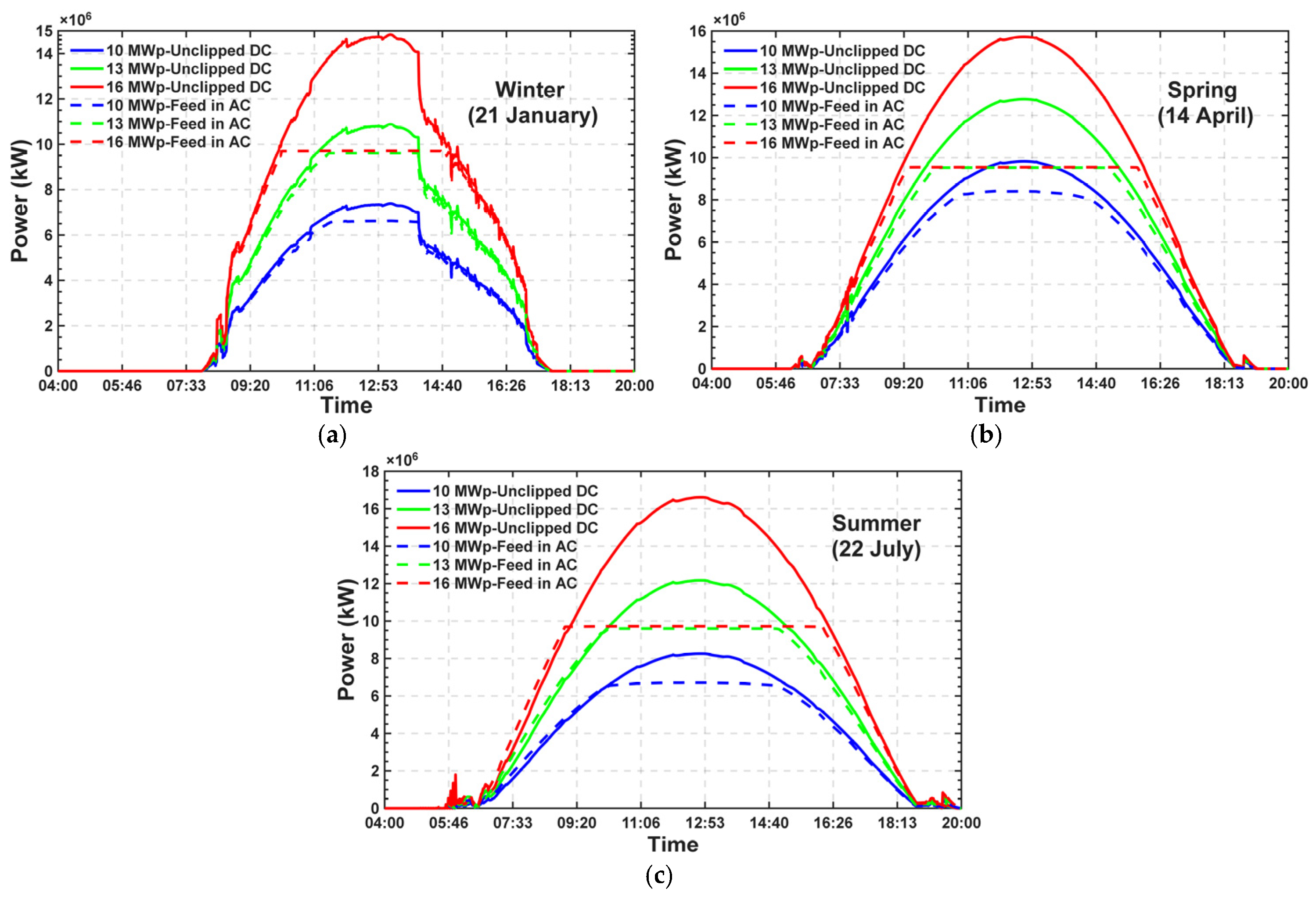
Figure 7a, which reflects the 21 January data for the winter season, shows that, due to low irradiance and shorter daylight hours, the system with the standard 10 MWp design operates well below the nominal inverter limit. During this period, increasing the installed DC power to 13 MWp and 16 MWp (oversizing) proportionally increases the inverter input power, compensates for the characteristically low energy yield in the winter months, and maximizes the total energy delivered to the grid without clipping losses.
Figure 7b, which reflects the spring season data for 14 April, shows that the DC power generation reaches its highest instantaneous peak values of the year, as optimum module temperature and high solar irradiance conditions coincide. Under these conditions, the DC power produced by the 13 MWp and 16 MWp systems rapidly exceeds the 10 MWe inverter limit around midday, resulting in a distinct clipping region (plateau). This plateau demonstrates that, in oversized systems, the inverter operates at full capacity for a considerably longer period than in the standard system, while the power curve becomes flatter, resulting in a more stable power profile at the grid connection point.
Figure 7c, which reflects the summer-season data for 22 July, shows that, despite longer daylight hours, the instantaneous peak DC power remains relatively lower than in the spring months due to thermal losses associated with increased ambient and module temperatures. However, the 13 MWp and 16 MWp systems, with their higher DC/AC ratios, exhibit a relatively wide power plateau, operating at the 10 MWe inverter capacity limit from the early morning hours until late afternoon.
As a result, these profiles clearly reveal that, although the increasing DC/AC ratio leads to midday clipping losses in the periods of the year with high solar potential, it supports generation during the morning/evening shoulder hours and in the winter months, substantially improving the capacity factor of the plant and the economic return of the investment.
7. Discussion
7.1. Simulation Accuracy and Model Reliability
The simulation results, in which the Edikli PVPP was modeled exactly with 15.237 MWp of installed power and 10 MWe of licensed power, reproduce the actual 2021 data obtained from the SCADA system within 2.66% in terms of annual total energy generation and within 1.93% in terms of performance ratio; the annual specific yield is not reported separately, because at a given installed capacity it is the annual energy divided by the same installed power and its relative deviation is therefore identical to that of the annual energy. Because the simulation is driven by a long-term climate dataset covering 2001–2020 while the measured record covers the single year 2021, the comparison is a long-term yield consistency check and not a measurement of model error, and the residual cannot be separated from interannual weather variability with one year of observation. The monthly deviations range in magnitude from 0.46% to 16.72% while the annual deviation is 2.66%; a deviation of this magnitude is in line with what has been reported for PV*SOL, where deviations between monitored and simulated annual production of 3–13%, with an average of 9%, have been found and the software has been observed to underestimate the electricity generated [61]. The monthly and annual deviations obtained here, together with the long-term character of the climate dataset, support the use of PVSOL in the feasibility analyses on which long-term investment decisions are based, provided that the time base of the comparison is stated.
The findings show that the modeled performance ratio (74.84%) and the value calculated from SCADA (76.31%) fall within the same band as the value of 75.7% reported for a grid-connected rooftop system in Türkiye [62]. The values obtained are also consistent with the performance ratios reported for different climates and technologies: the range of 77–85% for grid-connected plants [27], 0.78 at rooftop scale [25], and ~0.83 for a large-scale plant [1] have been reported. This comparison should be evaluated by taking into account the difference in scale (a 10 MWe ground-mounted plant versus a 24 kWp rooftop system) and differences in climate zone; nevertheless, the closeness of the values indicates that the energy performance obtained is consistent both regionally and methodologically. The comparison of the simulation outputs with empirical data produced in different contexts strengthens the reliability of the model by showing the consistency of indicators such as the capacity factor and energy yield [63]. Considering that the performance ratio is a widely accepted indicator in the international literature for comparing grid-connected plants [64], this result strengthens the external validity of the method.
7.2. Clipping Behavior and the Position of the Optimum DC/AC Ratio
The hypothesis of the study was that selecting a DC installed power above the licensed power and applying power limitation would ensure more efficient use of capacity and a shortening of the payback period. The results support this hypothesis, while showing that the benefit decreases after a certain DC/AC ratio. When the DC/AC ratio is greater than 1.0, the inverter is considered to be sized below its nominal AC power, and clipping arises together with a flattening effect in the daily production profile [10]. This phenomenon is explained by the output curve taking on a “flat-topped” form instead of a normal distribution when the inverter reaches its maximum output power [15]; it is stated that oversizing aims to increase the capacity factor and energy yield and to reduce the LCOE, while clipping is its inevitable side effect [17]. This situation directly overlaps with the “flat-topped” profile observed in the AC output curves of the 13 and 16 MWp models in Figure 7 and with the area between DC and AC. Increasing the installed DC power from 10 MWp to 16 MWp raises the energy transferred to the grid by only approximately 41.9%, while carrying the clipping loss from less than 0.01% to 13.38%; this asymmetry quantitatively reveals that an increasingly larger portion of the increasing DC capacity cannot be converted.
The optimum ratio obtained (DC/AC 1.275–1.30, that is, the 12.75–13.00 MWp configurations) is consistent with a wide band in the literature. The review study on the inverter sizing ratio states that the recommended DC/AC ratios are mostly concentrated between 1.1 and 1.5, and that a range of 1.19–1.287 with a cost minimization approach and 1.47 for Saudi Arabia have been reported [15]. Within this framework, the band of 1.275–1.30 found for Edikli is positioned within the 1.1–1.5 band, with its upper end just above the 1.19–1.287 range based on cost minimization, while the band remains below the value of 1.47 recommended for arid/high-irradiance regions. Recent studies broaden this picture: it has been reported that the optimum DC/AC ratio that minimizes clipping loss generally lies between 1.2 and 1.3 [32], that the optimum ILR for crystalline silicon and m-Si technologies is 121–130% (average 126%) [27], and that there is a global minimum point corresponding to an optimum ratio of 1.287 under cost minimization [15]. On the other hand, lower values such as 1.19 for the inverter power sizing ratio [26] and a range of 1.63–1.87 for a residential system in Valencia [30] have been reported. The optimum ratio also depends on the design objective of the system: when the highest specific yield is targeted, a value around 1.2 comes to the fore, while when the best financial outcome is targeted, the 1.3–1.6 band comes to the fore [11]. These differences show that there is no single universal optimum; the optimum ratio depends on project-specific variables such as climate, tariff structure, and scale [65]. Indeed, it is emphasized that the optimum sizing ratio depends on geographical location, inverter characteristics, and module technology [15]. Therefore, the band of 1.275–1.30 determined for Edikli should be regarded as a regional finding that confirms the “optimal according to circumstances” approach in the literature.
The band determined here is consistent with the results obtained for utility-scale systems: the LCOE of a 50 MW system decreases up to an inverter loading ratio of about 1.3–1.4 [66], and the ratio that minimizes the LCOE was found to lie between 1.1 and 1.3 for modern medium- and high-power inverters across 27 Brazilian cities [67]. The same design quantity has also been treated as a linear programming problem for a utility-scale plant operating under a feed-in tariff, where a reduction in the ILR from 1.4656 to 1.4528 was found to raise the annual profit annuities [68].
The seasonal structure of clipping is also consistent with the literature [32]. It is known that high DC/AC ratios increase production during the early and late hours of the day, but that the inverter is limited under full-load conditions [14]. In this study, clipping was concentrated, as expected, in the summer period, when irradiation is highest, and at midday; under winter conditions, however, clipping almost disappeared because the 10 MWe limit was not reached. It is also reported in the literature that the clipping loss exhibits a seasonal dependence and generally reaches its highest value at midday in summer, when irradiation is highest [32]. The fact that the effect of clipping on annual production remains limited because standard test conditions are rarely met during the year, but grows rapidly as installed DC power increases, is the main reason for the non-linear relationship between installed power and clipping; similarly, it has been shown that clipping regions are concentrated in a small portion of annual production and that the annual energy difference remains limited [9]. Within a given configuration, clipping loss lowers the performance ratio by removing delivered energy from the numerator of Equation (6), and it should therefore be taken into account when the ratio is interpreted [24]; the reduction is acceptable when sizing is done consciously and an optimum DC/AC ratio is selected [17]. This explains the decline of the PR values in the study from 82.21% to 72.91% together with installed power, and it is the opposite of the masking effect of Section 1.2, where the measured PR overstates the plant’s actual DC-side performance [1].
7.3. Interpretation of Economic Indicators and Their Balance with Technical Performance
The most important finding of the study is that the technical performance indicators and the economic indicators point to different installed power values. While the annual specific yield and the performance ratio reach their highest values in the lowest-capacity models (10–11 MWp), the shortest payback period (9.42 years) and the highest IRR (12.32%) were obtained in the 12.75–13.00 MWp models; the lowest cost of energy was also calculated as 0.0823 USD/kWh in the 12.50–13.00 MWp range. This divergence shows that investment decisions should not be based solely on production or efficiency indicators, but that indicators such as the payback period, IRR, NPV, and LCOE should be evaluated together. Indeed, integrated assessments in which these four indicators are used together are recommended in the literature [69], different cost criteria such as the NPC, LCOE, and life-cycle cost are used together in economic feasibility studies [3], and it is emphasized that the DPB is a more realistic measure of the initial investment compared with the simple payback method [70].
The NPV completes this picture. It rises to a maximum of USD 4,429,253 at 14.25 MWp (DC/AC 1.425), above the 12.75–13.00 MWp indicated by the payback period, the IRR and the LCOE, and it varies by USD 423,070, or 9.6% of its maximum, over the 12.00–14.00 MWp range, within which the three other indicators remain within 0.9% of their best values. The criterion that weights the later cash flows least heavily therefore points to the highest installed DC power, in line with the observation that the system with the highest NPV is not always the system with the lowest LCOE.
The divergence of the technical and economic optimum is also reported in the literature as a general phenomenon: in the example of a 100 MVA plant, it has been shown that the technical optimum based on the performance ratio remains at approximately a 130% DC/AC ratio, while the economic optimum in terms of NPV and IRR shifts to approximately a 170% DC/AC ratio [23]. The fact that different economic criteria point to different configurations strengthens this picture; in a battery-supported bifacial system, the fastest payback highlights the DC/AC ratio range of 1.0–1.05, the highest NPV the range of 1.1–1.3, and the lowest LCOE the range of 1.1–1.4 [18]. Similarly, it is stated that the system with the highest NPV is not always the system with the lowest LCOE, because each financial indicator reflects a different value of the system [32]. Therefore, the deviation of the economic optimum determined for Edikli, at 12.75–13.00 MWp (DC/AC ≈ 1.275–1.30), from the 10–11 MWp range indicated by the technical indicators is consistent with the literature. The position of that economic optimum is conditional on the cost-scaling rule of Section 5, as Section 6.2 shows.
The LCOE obtained at the optimum (0.0823 USD/kWh) is within 2% of the value of about 0.084 USD/kWh reported for a grid-connected PV system in an emerging economy, for which a payback period of about 10 years and an IRR of 8% are given [63]. The difference in scale (173 kWp in that study against 13 MWp here) and in tariff regime should be taken into account in this comparison. It should further be noted that the LCOE of the present study is computed with a real discount rate of 8% over a 25-year assessment period, and that it is therefore not directly comparable with levelized costs reported under other financial assumptions. On the other hand, the IRR of 8% reported for that system is lower than the value obtained here (12.32%), and the difference can be explained by the three-tier electricity sale tariff structure applied in this study (incentivized for the first five years, non-incentivized for the second five years, free market for the remaining 15 years) and by the difference in installed power scale [63]. This reveals that financial indicators are highly sensitive to the tariff regime and discount assumptions. Indeed, sensitivity analyses show that changes in the discount rate, installation cost, and especially the electricity sale price create a marked effect on all economic indicators, and that market conditions and tariff structures play a critical role in the feasibility of the investment [1]; it is also emphasized that project profitability is highly sensitive to retail electricity tariffs, net metering mechanisms, and incentives, and that a reduction in incentives can extend the payback period and pull the IRR below investor expectations [57].
In the cost model, the classification of an item as dependent on installed power or as fixed directly affects the results for items with a large share in the total investment. The land cost and the project development and engineering items are in this group. The land cost was associated with DC capacity because the land requirement depends on the number of modules and therefore on the installed DC power; the calculation of the lease amount on the basis of a fixed unit price per hectare makes this item directly proportional to the project scale [1]. The project development and engineering item, however, does not increase fully linearly with scale and may behave partly as fixed. If these items had been considered fixed, independent of installed power, the sensitivity of CAPEX to DC capacity would decrease; low-DC-capacity scenarios would become relatively expensive, and high-DC-capacity scenarios relatively cheap. In this case, the optimum indicated by the economic indicators would be expected to shift toward higher DC/AC ratios. Since it is known that cost and production magnitudes vary according to location, capacity, and project complexity, the transparent reporting of the classification decisions for items with a large share is necessary for the transferability of the results [16].
7.4. Policy and Environmental Context
The findings show that, in regulatory frameworks in which the licensed power is defined on the AC side and capacity overshoot is not permitted, selecting the DC/AC ratio above 1.0 is a rational design strategy from the investor’s perspective. This strategy increases the income obtained from the permitted AC capacity while also guaranteeing that the legal limit is not exceeded; if the installed power remains constant, however, an economic loss arises because the licensed capacity cannot be utilized sufficiently. The fact that designers size the inverter so as to minimize the life-cycle cost and accept the clipping loss, while also observing the upper limits imposed by transformer capacity and the AC grid connection, reflects this approach [14]; a typical example of regulatory constraints is rules stipulating a minimum DC/AC ratio of about 1.43 (AC/DC < 0.7 in the source’s notation) in order to smooth grid integration and allow for greater hosting capacity in the grid [12]. On the other hand, in markets where the DC/AC ratio is liberalized and the grid connection is the limiting factor, oversizing has become widespread in order to increase production, and a ratio in the range of 1.0–1.8 has been recommended in Chinese design guidelines; this approach reduces peak shaving pressure by creating a flat and high output at midday and lowers the installation cost through the sharing of equipment such as cables, inverters, and box transformers [71]. The fact that declining PPA prices make oversizing more attractive also supports this tendency [23]. Considering that the decline in module prices due to scale and cost reduction generally raises DC/AC ratios and that this can lead to clipping losses being overlooked [8], it is considered that the band determined by this study for the Edikli PVPP (DC/AC 1.275–1.30; 12.75–13.00 MWp, within the economically viable range of 1.20–1.40) can be guiding in practice.
From an environmental perspective, the CO2 emissions avoided by the modeled plants rise from 7799 t CO2/year to 11,066 t CO2/year together with installed power; the calculation of avoided emissions on the basis of the national grid emission factor is an approach widely used in such assessments [63]. The absolute reduction and the reduction per unit are not the same quantity, and they do not point to the same configuration. Because the emission factor is applied as a constant, the absolute avoided emissions are proportional to the energy delivered to the grid and rise monotonically from 7799 to 11,066 t CO2/year between 10 and 16 MWp, an increase of 41.9%; measured per unit of installed capacity the same quantity declines instead, from 0.780 to 0.692 t CO2/kWp.year, following the specific yield, and measured per unit of investment it rises by 5.3%, from 612.5 to 645.0 t CO2 per million USD, because the specific investment cost falls faster than the specific yield and the ratio reaches its maximum of about 661 t CO2 per million USD at 13.00 MWp. The avoided-emissions indicator is therefore monotonic in installed DC power and has no interior optimum: among the 25 configurations, it favors the largest one, which also carries the highest clipping loss, and not the configuration in which the clipping loss is minimized. Eliminating clipping is accordingly not in itself the criterion of an ecologically ideal design; it is the absolute reduction that increases with installed DC power while the reduction per unit of capacity decreases, and the two must be reported separately; it has also been shown that the clipped energy can be recovered through storage and that energy storage integration can reduce CO2 emissions [8].
7.5. Limitations and Future Research Directions
The findings of this study were obtained under the climatic conditions of a single location (Niğde/Edikli), a specific module–inverter configuration, and a defined tariff–tax scenario; therefore, caution should be exercised in generalizing the results. Nevertheless, the findings support the general acceptance that the optimum DC/AC ratio varies according to climate and cost structure, and they offer a methodological framework that should be repeated for different regions. Indeed, it has been shown that the threshold ratio at which clipping begins can rise to approximately 1.25 in regions receiving more irradiation and with less shading, and to as high as 1.35 in cloudy climates or under non-ideal orientations [25]; it has been reported that the optimum ratio varies depending on irradiation intensity and that even higher DC/AC ratios can remain optimal in low-irradiance regions [18].
One of the distinctive methodological features of this study is that the simulations were run at a 1 min time step rather than hourly. It has been reported that hourly resolution models can underestimate inverter clipping losses in climates with high cloudiness [72]; it is stated that hourly data can smooth short-term irradiation peaks and thereby shift the optimum array–inverter sizing ratio too high and lead to undersized inverters [29], and that clipping cannot be effectively estimated with hourly simulations and can occur even at time scales below 1 min [12]. Working at minute resolution enables such short-term irradiation peak values and the associated limitation behavior to be captured. The comparison with hourly approaches indicates the direction in which a coarser resolution errs, but it does not establish a bound on the result. Hourly simulations are ineffective at estimating clipping losses, which occur on a much shorter timescale [12], and clipping is the factor that limits the annual DC/AC conversion efficiency once the inverter operates at full load [29]. The one-minute step is therefore the resolution required to represent the limitation behavior, and the clipping losses reported in Table 12 are the values obtained at that resolution; they are not presented as an upper limit, because a shorter simulation step by itself does not establish such a constraint. In addition, the classification decisions in the cost model can affect the results for items with a high share in the total investment.
Another methodological contribution is the item-based cost model, which decomposes the CAPEX into the Table 10 items, classifies each by its dominant DC or AC dependence, and expresses the DC-dependent component as a linear function of installed power while the AC-dependent and capacity-independent components remain constant (Equations (2)–(4)). This rule is price-level-neutral: the 2020 prices are numerical inputs only, whereas the mechanism linking CAPEX to DC capacity—and hence the direction in which the optimum moves—holds for any level of the Category B prices, unlike the generalized USD/kWp method, which shifts all derived indicators without showing which cost is sensitive to oversizing [16]. Because 67.7% of the investment is DC-dependent (PV modules 27.72%, mechanical structures 9.04%) and 32.1% AC-dependent (license fee 23.16%, transmission line 3.50%), Category B has been the item group requiring re-pricing when cost data are updated. It should be noted, however, that the Category A and C items may also have moved since 2020: they correspond largely to balance-of-system and soft costs—land acquisition, site preparation, labor, permitting and grid connection [7]—which are country-specific rather than internationally priced and have declined at a slower rate than modules and at different rates across markets, with the balance of system now accounting for the majority of PV CAPEX [2]. A full update therefore requires re-pricing all three categories, A and C from current local cost components and B from current equipment prices. Since A and C are held constant across the 25 scenarios, it is the Category B price that governs the marginal cost of added DC capacity, whereas a re-pricing of A and C enters every scenario as the same absolute amount and acts on the level. The level is not neutral for the ratio-based indicators. A common amount reduces the net present value of every scenario by the same sum, so that the differences between scenarios—and with them the incremental comparison of two configurations—are unchanged; but the same amount is divided by a discounted lifetime energy that grows by 41.9% between 10 and 16 MWp, so that a 10% re-pricing of A and C (USD 536,250, 3.23% of the as-built CAPEX) raises the LCOE by 0.0033 USD/kWh at 10 MWp and by 0.0023 USD/kWh at 16 MWp, and it corresponds to 4.21% of the capital sum at 10 MWp against 3.13% at 16 MWp, so that it lengthens the DPB and lowers the IRR by more, in relative terms, for the smaller arrays. The ratio-based optimum is therefore conditional on the price level of these items: over the flat region the LCOE minimum is attained by the configurations 12.50–13.00 MWp in the base case, by 12.50–12.75 MWp with a 10% reduction and by 12.75–13.25 MWp with a 10% increase, so that the plateau moves by one step in the direction of the re-pricing, and the band reported in Section 6.2 is valid for their 2020 values. The position of the optimum depends more strongly on the rule than on the price level: across the four cost structures tested it ranges from 10.50–11.00 MWp under the constant-cost-per-kWp rule to 15.25 MWp with all four site items fixed.
Because the AC capacity in this study was limited to the licensed AC power, the Category C cost was held constant: the plant cannot expand its AC-side capacity beyond the licensed value, so the license fee and the transmission line cost do not vary with the DC capacity examined. This assumption is what makes the model directly applicable to the plant as licensed. Its application to a different AC capacity would follow the same logic: if the licensed AC power or the grid connection arrangement were to change, the Category C items would be re-priced from the updated components—the license fee from the new licensed capacity and the transmission line from the new connection arrangement—and their revised weight within the CAPEX (currently 23.16% and 3.50%, together 32.1%) recomputed. A larger AC capacity would reduce the clipped energy, and hence the marginal energy gain from each additional MWp of DC capacity, while raising the fixed AC-side share, so the trade-off between added cost and recovered energy would be re-established on new terms; the same 10–16 MWp scenario set could then be re-run with the updated Category C values.
All costs and tariffs are at the 2020 price level and no price index is applied, so that the Table 12 indicators are valid for that price level. A nominal treatment would return the same real indicators if every monetary term were escalated by one and the same index and the discount rate were converted to the corresponding nominal rate. The assumption that the three tariff blocks preserve their 2020 purchasing power, rather than declining in real terms as nominally fixed tariffs would, is stated in Section 6.1, together with the property that the levelized cost is insensitive to it because Equation (9) contains no tariff. Because only Category B responds to installed power, lower DC-side prices—which have already made array oversizing common practice [18]—reduce the marginal CAPEX of each additional MWp while the marginal energy gain (site irradiance, the 10 MWe limit, the resulting clipping loss) is unchanged; revenue would then exceed cost over a longer 10–16 MWp range, and the optimum would be expected to shift above the 1.275–1.30 determined here, widening the divergence from the technical optimum, whereas higher DC-side prices would pull it back towards the 10–11 MWp indicated by the technical indicators. Specific investment cost already falls from USD 1273.37/kWp at 10 MWp to USD 1072.28/kWp at 16 MWp as fixed costs spread over a larger DC capacity.
Two limitations concern the validation directly. The first is the time base of the comparison: the simulation is driven by a long-term climate dataset covering 2001–2020 while the measured record covers the single year 2021, so the comparison establishes long-term yield consistency rather than model accuracy, and the separation of model error from interannual variability would require a multi-year measurement series together with a year-specific climate input. The second is the resolution of the measured data: the values available for this plant are monthly, and records at a finer time resolution, together with operational records of outages, maintenance and curtailment, are not available to the authors. The power limitation of the inverters therefore cannot be validated interval by interval, and the clipping loss reported by the model cannot be checked against a measured time spent in clipping mode, although that time can be recorded directly by the inverter or the monitoring system. The modeling of the limitation is performed at a 1 min time step, which is the resolution required to resolve clipping, but this concerns the model and not the measurement; the interval-level validation of clipping remains to be carried out on a plant for which sub-hourly measured data are available.
A further boundary concerns the climate input rather than the measurement: the one-minute step resolves the bulk of the variability relevant to clipping, but events shorter than one minute, such as brief cloud enhancement peaks, are not resolved.
A further limitation concerns the electrical compatibility check of Section 5: the input current reported there is derived from the data sheets of Table 4 and Table 5 and is not measured at the MPP input of the plant, and the MPP input current tolerance differs among inverter models, so that the check is specific to the inverter used.
Two limitations attach to the quantification of the degradation–clipping interaction reported in Section 6.1 and Table 14. The current-reduced module used in that check is a proxy and not identical to a physically smaller array, since it retains the module count and the string voltage of the as-built arrangement, so that its cable losses are lower than those of a 10.40 MWp array and its specific yield of 1687.40 kWh/kWp exceeds the 1659–1660 kWh/kWp of the 10–11 MWp configurations of Table 12; the recovered energy is therefore an estimate of the order of magnitude rather than an exact value. In addition, the interaction was quantified at the optimum configuration rather than by re-running all 25 arrays at end-of-life power, and full re-optimization in which the interaction is represented inside the cash flow model is left to future work.
A further approximation concerns the export control itself: the 10 MWe limit is applied at the inverter and not at the metering point, so that the modeled export remains about 2.9% of the licensed power below the limit at the point where the license applies, and the transformers and the MV connection, whose losses lie downstream of the LV busbar at which both the model and the SCADA comparison terminate, are not represented as loss items.
Two directions come to the fore for future studies. The first is the techno-economic analysis of making the clipped energy usable through storage systems; it is known that a storage unit to be positioned on the DC bus can recover the clipped energy and allow for higher DC/AC ratios [8]. The second is the investigation of the effect of bifacial modules and long-term module degradation on clipping and financial indicators. It is reported that, despite the potential of bifacial modules to reduce the DC/AC ratio relative to nominal power thanks to their ability to benefit from reflected irradiation, they can nearly double the clipping losses at the same ratio compared with a monofacial configuration, while producing more energy over their lifetime [17]. In addition, it is anticipated that reducing the wiring loss, calculated as 4.49% in the existing plant, through an increase in cross-section will improve the financial indicators; it is known that the use of thicker conductors can reduce DC wiring loss from the level of 2% to 1% [25].
8. Conclusions
In this study, a licensed solar power plant with 15.237 MWp of installed DC power and 10 MWe of licensed AC power, operating in the Edikli district of the province of Niğde and applying power limitation, was examined from technical and economic perspectives. Unlike the generalized kWp-based cost approach commonly used in the literature, a detailed cost model was used in which the items affected and unaffected by the change in installed power were separated. The analyses were carried out at a 1 min resolution via PVSOL software.
In the first stage of the study, the plant was modeled exactly and the simulation results were compared with the SCADA data. The results showed that the annual energy delivered to the grid agrees with the measured record of 2021 to a relative deviation of −2.66% and the performance ratio to −1.93% in a long-term yield consistency check between a simulation driven by a climate dataset covering 2001–2020 and the measurement of a single year. In the second stage, 25 different modelings with DC/AC ratios varying in the range of 1.0–1.6 were carried out; it was determined that when the installed power was increased from 10 MWp to 16 MWp, the energy transferred to the grid increased by approximately 41.9%, while the clipping loss rose from less than 0.01% to 13.38%. The results reveal that the DPB (9.42 years), the IRR (12.32%) and the LCOE (0.0823 USD/kWh) reach their best values jointly at 12.75–13.00 MWp (DC/AC 1.275–1.30). Because the three indicators vary only slightly between neighboring configurations, the result is reported as the economically viable range of 12.00–14.00 MWp (DC/AC 1.20–1.40), within which all three remain within 0.9% of their best values. The position of this range is conditional on the item-based cost-scaling rule: under the constant-cost-per-kWp model, the same three optima lie at 10.50–11.00 MWp. The NPV at a real discount rate of 8% reaches its maximum of USD 4,429,253 at 14.25 MWp and therefore favors the upper part of that range. The main findings of the study can be summarized as follows:
- PVSOL is a reliable simulation tool in the feasibility studies of PV systems that will operate under the climatic conditions of Niğde/Edikli, reproducing the measured annual energy generation to a relative deviation of −2.66% and the measured performance ratio to −1.93%, provided that the comparison between a long-term climate dataset and a single year of measurement is reported as a long-term yield consistency check.
- Since climatic conditions rarely provide standard test conditions during the year, PVPPs are often unable to produce at their installed power values.
- In licensed power plants, selecting a DC/AC ratio above 1.0 and applying power limitation in order to benefit from the licensed power at the highest level provides an economic advantage and shortens the payback period.
- The optimum DC/AC ratio varies according to the climatic conditions of the installation region; the most suitable ratio for Niğde/Edikli was determined as DC/AC 1.275–1.30 (12.75–13.00 MWp), within the economically viable range of DC/AC 1.20–1.40 (12.00–14.00 MWp). Its position is conditional on the item-based cost-scaling rule applied here; a fixed share in half or all of the four site items places it at 13.50–14.00 and 14.50–15.25 MWp.
- While the technical performance indicators (annual specific yield and performance ratio) reach their highest values in the 10–11 MWp models, the economic indicators (payback period, IRR, LCOE) converge on the 12.75–13.00 MWp range, corresponding to DC/AC 1.275–1.30, which lies within the economically viable range of 12.00–14.00 MWp (DC/AC 1.20–1.40); therefore, investment decisions should be based on the joint evaluation of these indicators.
- The modeled plants avoid between 7799 and 11,066 tons of CO2 per year, and the widespread adoption of solar power plants offers important contributions in terms of reducing the carbon footprint and ensuring sustainable environmental conditions.
Supplementary Materials
The following supporting information can be downloaded at: https://www.mdpi.com/article/10.3390/pr14223693/s1. Table S1. Sensitivity analysis.
Author Contributions
Conceptualization, S.S.; methodology, A.S. and S.S.; software, A.S. and S.S.; validation, A.S. and S.S.; formal analysis, A.S. and S.S.; investigation, A.S. and S.S.; resources, A.S.; data curation, A.S.; writing—original draft preparation, S.S.; writing—review and editing, A.S. and S.S.; visualization, A.S. and S.S.; supervision, S.S. All authors have read and agreed to the published version of the manuscript.
Funding
This research received no external funding.
Data Availability Statement
The data supporting the findings of this study are included in this article. The aggregated monthly and annual generation data are reported in full within the manuscript. The measured data available for the plant are monthly energy values recorded by the SCADA system; records at a finer time resolution, and operational records of outages, maintenance and curtailment, are not available to the authors. The monthly error metrics reported in Section 4 are derived from the monthly values presented in Figure 5.
Acknowledgments
We would like to express our sincere thanks to Levent Gülbahar, General Manager of Birleşim Grup Enerji A.Ş., and to Mesut Altan, Chairman of the Board of Directors of Birleşim Grup, for their permissions and contributions regarding the provision of the technical data of the Edikli PVPP addressed in this study. During the preparation of this study, the authors used Jenni.ai for the purposes of translating the text into English, language editing, formatting the manuscript in accordance with the journal’s submission requirements, and assisting in the analysis and interpretation of the data. The authors have reviewed and edited the output and take full responsibility for the content of this publication.
Conflicts of Interest
The authors declare the following competing interests: Author A.S. is employed by Erde Mühendislik A.Ş. and supplied the technical and cost data of the plant analyzed in this study; the employer and the plant operator, Edikli GES Enerji A.Ş., are both companies of Birleşim Grup. The remaining author declares no competing interests.
Abbreviations
The following abbreviations are used in this manuscript:
| CAPEX | Capital Expenditure |
| CEA | Avoided CO2 Emission |
| DHI | Diffuse Horizontal Irradiance |
| DPB | Discounted Payback Period |
| EPC | Engineering, Procurement, and Construction |
| EPDK | Energy Market Regulatory Authority |
| GEPA | Türkiye Solar Energy Potential Atlas |
| GHI | Global Horizontal Irradiance |
| ILR | Inverter Loading Ratio |
| IRR | Internal Rate of Return |
| LCOE | Levelized Cost of Energy |
| LFP | Lithium Iron Phosphate |
| LV | Low Voltage |
| MCCB | Molded Case Circuit Breaker |
| MPPT | Maximum Power Point Tracker |
| m-Si | Monocrystalline Silicon |
| MV | Medium Voltage |
| NPC | Net Present Cost |
| NPV | Net Present Value |
| O&M | Operation and Maintenance |
| PERC | Passivated Emitter and Rear Contact |
| PPA | Power Purchase Agreement |
| PR | Performance Ratio |
| PV | Photovoltaic |
| PVGIS | Photovoltaic Geographical Information System |
| PVPP | Photovoltaic Power Plant |
| SAM | System Advisor Model |
| SCADA | Supervisory Control and Data Acquisition |
| STC | Standard Test Conditions |
| T2m | Mean 2-Meter Air Temperature |
| TEDAŞ | Turkish Electricity Distribution Corporation |
| TEİAŞ | Turkish Electricity Transmission Corporation |
| TS | Transformer Substation |
| WS2m | Mean 2-Meter Wind Speed |
| YEKA | Renewable Energy Resource Area |
| YEKDEM | Renewable Energy Resources Support Mechanism |
References
- Thom, D.; Bugała, A.; Bugała, D.; Czekała, W. Comprehensive Energy and Economic Analysis of Selected Variants of a Large-Scale Photovoltaic Power Plant in a Temperate Climate. Energies 2025, 18, 4198. [Google Scholar] [CrossRef] [Scilit]
- Elshurafa, A.M.; Albardi, S.R.; Bigerna, S.; Bollino, C.A. Estimating the Learning Curve of Solar PV Balance–of–System for over 20 Countries: Implications and Policy Recommendations. J. Clean. Prod. 2018, 196, 122–134. [Google Scholar] [CrossRef] [Scilit]
- Alsadi, S.; Khatib, T. Photovoltaic Power Systems Optimization Research Status: A Review of Criteria, Constrains, Models, Techniques, and Software Tools. Appl. Sci. 2018, 8, 1761. [Google Scholar] [CrossRef] [Scilit]
- 6446 Sayılı Elektrik Piyasası Kanununun 16 Ncı Maddesi Uyarınca Yıllara Sair Uygulanacak Para Cezaları Hakkında Tebliğler. Available online: https://www.epdk.gov.tr/Detay/DownloadDocument?id=Un5fnwdIgpI= (accessed on 5 October 2026).
- Big-Alabo, A. Review of Deep Reinforcement Learning Algorithms for MPPT and Partial Shading in Solar PV Applications. J. Adv. Eng. Comput. 2026, 10, 84. [Google Scholar] [CrossRef] [Scilit]
- Akai, K.A.; Kuku, R.O.; Sobamowo, G.M.; Raji, N.A. Numerical Investigation of Solar Cell Temperature for a Concentration of Photovoltaic System. J. Adv. Eng. Comput. 2025, 9, 123. [Google Scholar] [CrossRef] [Scilit]
- Victoria, M.; Haegel, N.M.; Peters, I.M.; Sinton, R.A.; Jäger-Waldau, A.; del Cañizo, C.; Breyer, C.; Stocks, M.; Blakers, A.; Kaizuka, I.; et al. Solar Photovoltaics Is Ready to Power a Sustainable Future. Joule 2021, 5, 1041–1056. [Google Scholar] [CrossRef] [Scilit]
- Demirci, A.; Öztürk, Z.; Tercan, S.M.; Nakir, İ. Determination of Photovoltaic Inverter Ratio Minimizing Energy Clipping for Electric Vehicle Charging Station under Different Solar Radiations. In Proceedings of the 2022 International Congress on Human-Computer Interaction, Optimization and Robotic Applications (HORA), Ankara, Turkey, 9–11 June 2022; pp. 1–6. [Google Scholar] [CrossRef] [Scilit]
- Beyoğlu, M.F.; Demirtaş, M. Determination of Optimal DC/AC Ratio for Grid-Connected Photovoltaic Systems. Celal Bayar Üniversitesi Fen Bilim. Derg. 2023, 19, 19–29. [Google Scholar] [CrossRef] [Scilit]
- Wang, H.; Muñoz-García, M.Á.; Cantero, G.P.M.; Alonso-García, M.C. Optimum Inverter Sizing of Grid-Connected Photovoltaic Systems Based on Energetic and Economic Considerations. Renew. Energy 2017, 118, 709–717. [Google Scholar] [CrossRef] [Scilit]
- Zipp, K. Why Array Oversizing Makes Financial Sense. In Solar Power World; WTWH Media LLC: Cleveland, OH, USA, 2018; p. 12. [Google Scholar]
- Balfour, J.R.; Hill, R.; Walker, A.; Robinson, G.; Gunda, T.; Desai, J. Masking of Photovoltaic System Performance Problems by Inverter Clipping and Other Design and Operational Practices. Renew. Sustain. Energy Rev. 2021, 145, 111067. [Google Scholar] [CrossRef] [Scilit]
- Sangwongwanich, A.; Yang, Y.; Séra, D.; Blaabjerg, F.; Zhou, D. On the Impacts of PV Array Sizing on the Inverter Reliability and Lifetime. IEEE Trans. Ind. Appl. 2018, 54, 3656–3667. [Google Scholar] [CrossRef] [Scilit]
- İşin, E.; Çetinkaya, N. Determination of Optimum Dc/Ac Ratio for PV Power Plants Using Artificial Intelligence. In Proceedings of the 3rd International Word Energy Conference, Kayseri, Türkiye, 4–5 December 2023. [Google Scholar]
- Hazim, H.I.; Baharin, K.A.; Gan, C.K.; Sabry, A.H.; Humaidi, A.J. Review on Optimization Techniques of PV/Inverter Ratio for Grid-Tie PV Systems. Appl. Sci. 2023, 13, 3155. [Google Scholar] [CrossRef] [Scilit]
- Branker, K.; Pathak, M.; Pearce, J.M. A Review of Solar Photovoltaic Levelized Cost of Electricity. Renew. Sustain. Energy Rev. 2011, 15, 4470–4482. [Google Scholar] [CrossRef] [Scilit]
- de Souza Silva, J.L.; de Melo, K.B.; Costa, T.S.; Machado, G.M.V.; Moreira, H.S.; Villalva, M.G. Impact of Bifacial Modules on the Inverter Clipping in Distributed Generation Photovoltaic Systems in Brazil. In Proceedings of the 2021 Brazilian Power Electronics Conference (COBEP), João Pessoa, Brazil, 7–10 November 2021; pp. 1–6. [Google Scholar] [CrossRef] [Scilit]
- Kaewnukultorn, T.; Mora, S.B.S.; Hegedus, S. The Impacts of DC/AC Ratio, Battery Dispatch, and Degradation on Financial Evaluation of Bifacial PV+BESS Systems. Renew. Energy 2024, 236, 121402. [Google Scholar] [CrossRef] [Scilit]
- Ahmad, M.; Khattak, A.; Janjua, A.K.; Alahmadi, A.A.; Khan, M.S.; Ullah, N. Techno-Economic Feasibility Analyses of Grid- Connected Solar Photovoltaic Power Plants for Small Scale Industries of Punjab, Pakistan. Front. Energy Res. 2022, 10, 1028310. [Google Scholar] [CrossRef] [Scilit]
- Camps, X.; Velasco, G.; de la Hoz, J.; Martín, H. Contribution to the PV-to-Inverter Sizing Ratio Determination Using a Custom Flexible Experimental Setup. Appl. Energy 2015, 149, 35–45. [Google Scholar] [CrossRef] [Scilit]
- Eurek, K.; Murphy, C.A.; Cole, W.; Frazier, W.; Brown, P.D.; Schleifer, A.H. Representing DC-Coupled PV+Battery Hybrids in a Capacity Expansion Model; OSTI OAI (U.S. Department of Energy Office of Scientific and Technical Information): Oak Ridge, TN, USA; National Renewable Energy Laboratory (NREL): Golden, CO, USA, 2021. [Google Scholar] [CrossRef] [Scilit]
- Zidane, T.E.K.; Zali, S.M.; Adzman, M.R.; Tajuddin, M.F.N.; Durusu, A. PV Array and Inverter Optimum Sizing for Grid-Connected Photovoltaic Power Plants Using Optimization Design. J. Phys. Conf. Ser. 2021, 1878, 12015. [Google Scholar] [CrossRef] [Scilit]
- SMA Solar Technology AG. Maximum Freedom When Oversizing, Oversizing Whitepaper; SMA Solar Technology AG: Niestetal, Germany, 2018. [Google Scholar]
- Pandey, S.; Kumar, R.; Panwar, K. Calculation of Inverter Power Clipping Loss Due to PV Array Oversizing. Int. J. Electr. Eng. Technol. 2019, 10, 43–46. [Google Scholar] [CrossRef] [Scilit]
- Medojevic, M.; Medojević, M.; Diaz, V. Simulation-Based Design of Solar Photovoltaic Energy Generation System for Manufacturing Support. Therm. Sci. 2020, 25, 2517–2538. [Google Scholar] [CrossRef] [Scilit]
- Hazim, H.I.; Baharin, K.A.; Gan, C.K.; Sabry, A.H. Techno-Economic Optimization of Photovoltaic (PV)-Inverter Power Sizing Ratio for Grid-Connected PV Systems. Results Eng. 2024, 23, 102580. [Google Scholar] [CrossRef] [Scilit]
- Deschamps, E.; Rüther, R. Optimization of Inverter Loading Ratio for Grid Connected Photovoltaic Systems. Sol. Energy 2018, 179, 106–118. [Google Scholar] [CrossRef] [Scilit]
- Paiva, G.M.; Pimentel, S.P.; Marra, E.G.; Alvarenga, B.P. Analysis of Inverter Sizing Ratio for PV Systems Considering Local Climate Data in Central Brazil. IET Renew. Power Gener. 2017, 11, 1364–1370. [Google Scholar] [CrossRef] [Scilit]
- Rodrigo, P.M.; Velázquez, R.; Férnández, E.F. DC/AC Conversion Efficiency of Grid-Connected Photovoltaic Inverters in Central Mexico. Sol. Energy 2016, 139, 650–665. [Google Scholar] [CrossRef] [Scilit]
- Díaz-Bello, D.; Vargas-Salgado, C.; Águila-León, J.; Vargas, F.A.L. Methodology to Estimate the Impact of the DC to AC Power Ratio, Azimuth, and Slope on Clipping Losses of Solar Photovoltaic Inverters: Application to a PV System Located in Valencia Spain. Sustainability 2023, 15, 2797. [Google Scholar] [CrossRef] [Scilit]
- Buratynskyi, I.; Nechaieva, T.; Shulzhenko, S.V.; Ivanenko, N. The Optimization of PV-Plant’s DC/AC Equipment Ratio Using the Non-Linear Least-Cost Model. In Proceedings of the 2021 IEEE 3rd Ukraine Conference on Electrical and Computer Engineering (UKRCON), Lviv, Ukraine, 26 August 2021; pp. 358–362. [Google Scholar]
- Kaewnukultorn, T.; Mora, S.B.S.; Purnell, R.; Hegedus, S. Electrical and Financial Impacts of Inverter Clipping on Oversized Bifacial Photovoltaic Systems. Energies 2024, 17, 5658. [Google Scholar] [CrossRef] [Scilit]
- Bahloul, M.; Horan, D.; Khadem, S. Energy Storage Sizing Analysis and Its Viability for PV Power Plant Clipping Losses Minimisation. Electr. Power Syst. Res. 2023, 225, 109837. [Google Scholar] [CrossRef] [Scilit]
- Müller, N.; Kouro, S.; Zanchetta, P.; Wheeler, P.; Bittner, G.; Girardi, F. Energy Storage Sizing Strategy for Grid-Tied PV Plants under Power Clipping Limitations. Energies 2019, 12, 1812. [Google Scholar] [CrossRef] [Scilit]
- Yao, M.; Cai, X. Energy Storage Sizing Optimization for Large-Scale PV Power Plant. IEEE Access 2021, 9, 75599–75607. [Google Scholar] [CrossRef] [Scilit]
- Mikofski, M.A.; Holmgren, W.F.; Newmiller, J.; Kharait, R. Effects of Solar Resource Sampling Rate and Averaging Interval on Hourly Modeling Errors. IEEE J. Photovolt. 2023, 13, 202–207. [Google Scholar] [CrossRef] [Scilit]
- T.C. Enerji ve Tabii Kaynaklar Bakanlığı—Güneş. Available online: https://www.enerji.gov.tr/gunes-bilgimerkezi (accessed on 11 September 2026).
- Türkiye Solar Energy Potential Atlas. Available online: https://evcedyetkilendirme.enerji.gov.tr/Mycalculator/Default.aspx (accessed on 3 October 2026).
- T.C. 6446 Sayılı Elektrik Piyasası Kanunu. Available online: https://mevzuat.gov.tr/mevzuatmetin/1.5.6446.pdf (accessed on 7 October 2026).
- T.C. Elektrik Piyasası Lisans Yönetmeliği. Available online: https://www.epdk.gov.tr/Detay/Icerik/3-6727/elektrik-piyasasi-lisans-yonetmeligi (accessed on 7 October 2026).
- Şakar, İ.; Güngör, G.A. Enerjide Dışa Bağımlılığın Ekonomik Büyüme Üzerine Etkisi: Türkiye Üzerine Bir İnceleme. Ekon. VE Yönet. Araştırmaları Derg. 2025, 14, 2–40. [Google Scholar]
- Kavcioğlu, Ş. Yenilenebilir Enerji ve Türkiye. Finans. Araştırmalar VE Çalışmalar Derg. 2019, 11, 209–227. [Google Scholar] [CrossRef] [Scilit]
- Akdağ, V.; Gözen, M. Yenilenebilir Enerji Projelerine Yönelik Güncel Yatırım ve Finansman Modelleri: Karşılaştırmalı Bir Değerlendirme. Celal Bayar Üniversitesi Sos. Bilim. Derg. 2020, 139–156. [Google Scholar] [CrossRef] [Scilit]
- Pak, R.B.; Özdemir, E. Küresel İklim Mücadelesi Ekseninde Türkiye’nin Yeşil Enerji Dönüşümüne Genel Bir Bakış. Yekarum 2023, 8, 32–53. [Google Scholar]
- Yenilenebilir Enerji Kaynak Alanları Yönetmeliğinde Değişiklik Yapılmasına Dair Yönetmelik (RG 09.12.2025-33102). Available online: https://www.resmigazete.gov.tr/eskiler/2025/12/20251209-5.htm (accessed on 3 October 2026).
- Edikli PV Power Plant. Available online: https://birlesimgrupenerji.com/tr/yatirimlarimiz/edikli-nigde-ges (accessed on 3 October 2026).
- Uzar, M.; Koca, H. Güneş enerjisi santrallerinin yer seçimi için uygunluk haritasının oluşturulmasında klasik ve bulanık mantığa dayalı yöntemlerin analizi: Menemen örneği. J. Geod. Geoinf. 2020, 7, 11–28. [Google Scholar] [CrossRef] [Scilit]
- Soydan, O. Solar Power Plants Site Selection for Sustainable Ecological Development in Nigde, Turkey. SN Appl. Sci. 2021, 3, 41. [Google Scholar] [CrossRef] [Scilit]
- Demirkiran, M.; Karakaya, A. Efficiency Analysis of Photovoltaic Systems Installed in Different Geographical Locations. Open Chem. 2022, 20, 748–758. [Google Scholar] [CrossRef] [Scilit]
- Özden, T. A Countrywide Analysis of 27 Solar Power Plants Installed at Different Climates. Sci. Rep. 2022, 12, 746. [Google Scholar] [CrossRef] [Scilit]
- Limem, F.; Sezen, S. Comparative Analysis of Different Photovoltaic Simulation Software: Case Study on Analyzing the Performance of a 5,1 kWp Grid Connected Photovoltaic System. Eur. J. Sci. Technol. 2022, 32, 816–826. [Google Scholar] [CrossRef] [Scilit]
- PV*SOL Online Help. Module Temperature; Valentin Software: Berlin, Germany, 2026; Available online: https://help.valentin-software.com/pvsol/en/calculation/pv-modules/module-temperature/ (accessed on 26 October 2026).
- T.C. Enerji ve Tabii Kaynaklar Bakanlığı Türkiye Emisyon Faktörleri. Available online: https://enerji.gov.tr/evced-cevre-ve-iklim-elektrik-uretim-tuketim-emisyon-faktorleri? (accessed on 27 October 2026).
- Wang, Y.; Das, R.; Putrus, G.; Kötter, R. Economic Evaluation of Photovoltaic and Energy Storage Technologies for Future Domestic Energy Systems—A Case Study of the UK. Energy 2020, 203, 117826. [Google Scholar] [CrossRef] [Scilit]
- Lindahl, J.; Lingfors, D.; Elmqvist, Å.; Mignon, I. Economic Analysis of the Early Market of Centralized Photovoltaic Parks in Sweden. Renew. Energy 2021, 185, 1192–1208. [Google Scholar] [CrossRef] [Scilit]
- Stid, J.T.; Shukla, S.; Kendall, A.D.; Anctil, A.; Hyndman, D.W.; Rapp, J.; Anex, R.P. Impacts of Agrisolar Co-Location on the Food–Energy–Water Nexus and Economic Security. Nat. Sustain. 2025, 8, 702–713. [Google Scholar] [CrossRef] [Scilit]
- Kobashi, T.; Jittrapirom, P.; Yoshida, T.; Hirano, Y.; Yamagata, Y. SolarEV City Concept: Building the next Urban Power and Mobility Systems. Environ. Res. Lett. 2020, 16, 24042. [Google Scholar] [CrossRef] [Scilit]
- Joshi, S.; Mittal, S.; Holloway, P.; Shukla, P.R.; Gallachóir, B.Ó.; Glynn, J.D.M. High Resolution Global Spatiotemporal Assessment of Rooftop Solar Photovoltaics Potential for Renewable Electricity Generation. Nat. Commun. 2021, 12, 5738. [Google Scholar] [CrossRef] [Scilit]
- Ramírez, F.J.; Honrubia-Escribano, A.; Gómez-Lázaro, E.; Pham, D.T. Combining Feed-in Tariffs and Net-Metering Schemes to Balance Development in Adoption of Photovoltaic Energy: Comparative Economic Assessment and Policy Implications for European Countries. Univ. Birm. Res. Portal (Univ. Birm.) 2017, 102, 440–452. [Google Scholar] [CrossRef] [Scilit]
- Lai, C.S.; McCulloch, M. Levelized Cost of Electricity for Solar Photovoltaic and Electrical Energy Storage. Appl. Energy 2017, 190, 191–203. [Google Scholar] [CrossRef] [Scilit]
- Korsavi, S.S.; Zomorodian, Z.S.; Tahsildoost, M. Energy and Economic Performance of Rooftop PV Panels in the Hot and Dry Climate of Iran. J. Clean. Prod. 2017, 174, 1204–1214. [Google Scholar] [CrossRef] [Scilit]
- Caglayan, N.; Celik, H.K.; Asri, F.Ö.; Rennie, A.E.W. Experimental Validation and Performance Benchmarking of a Grid-Connected Rooftop Photovoltaic System Using Measured and Simulated Data. Energies 2026, 19, 1468. [Google Scholar] [CrossRef] [Scilit]
- Acosta-Banda, A.; Aguilar, V.H.; Difur, L.H.; Mercado, E.C.; Cortés-Martínez, B.; Patiño-Ortiz, M. Grid-Connected Photovoltaic Systems as an Alternative for Sustainable Urbanization in Southeastern Mexico. Urban Sci. 2025, 9, 329. [Google Scholar] [CrossRef] [Scilit]
- Saka, K. Evaluation of a Grid-Connected PV Power Plant: Performance and Agrivoltaic Aspects. Environ. Dev. Sustain. 2024, 26, 32319–32336. [Google Scholar] [CrossRef] [Scilit]
- Mounetou, R.; Alcantara, I.B.; Incalza, A.; Justiniano, J.; Loiseau, P.; Piguet, G.; Sabene, A. Oversizing Array-To-Inverter (DC-AC) Ratio: What Are the Criteria and How to Define the Optimum? EU PVSEC 2014, 2813–2821. [Google Scholar] [CrossRef] [Scilit]
- Denholm, P.; Margolis, R.; Eichman, J. Evaluating the Technical and Economic Performance of PV Plus Storage Power Plants; No. NTRL/TP-6A20-68373; National Renewable Energy Laboratory (NREL): Golden, CO, USA, 2017.
- Menezes, A.V.; Vieira Filho, J.d.A.A.; Macêdo, W.N. Challenges and Opportunities in ILR Selection for Photovoltaic System: Evaluation in Brazilian Cities. Energies 2025, 18, 2203. [Google Scholar] [CrossRef] [Scilit]
- Bahloul, M.; Khadem, S. A Refined Method for Optimising Inverter Loading Ratio in Utility-Scale Photovoltaic Power Plant. Energy Rep. 2024, 12, 5110–5115. [Google Scholar] [CrossRef] [Scilit]
- Fuster-Palop, E.; Vargas-Salgado, C.; Ferri-Revert, J.C.; Payá, J. Performance Analysis and Modelling of a 50 MW Grid-Connected Photovoltaic Plant in Spain after 12 Years of Operation. Renew. Sustain. Energy Rev. 2022, 170, 112968. [Google Scholar] [CrossRef] [Scilit]
- Yousuf, M.U.; Saleem, M.U.; Umair, M. Evaluating the 7E Impact of Solar Photovoltaic Power Plants at Airports: A Case Study. Sci. Technol. Energy Transit. 2024, 79, 19. [Google Scholar] [CrossRef] [Scilit]
- Xu, X.; Ma, C.; Gou, H.; Deng, Z.; Tian, Z. Controllable Joint Forecast of Oversized Photovoltaic-Energy Storage Systems Considering Energy Storage Flexibility. Energy 2025, 319, 135138. [Google Scholar] [CrossRef] [Scilit]
- Meyer, I.; Salles, A.; Julian, T.M.; Vorasitchai, V.; Sebastian, C.B.; Nonthi, C. Optimisation of DC/AC Ratio in Different Climatic Zones: A Technical Analysis on a Sub-Hourly Level. EU PVSEC 2020, 1610–1615. [Google Scholar] [CrossRef]
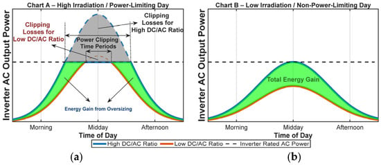
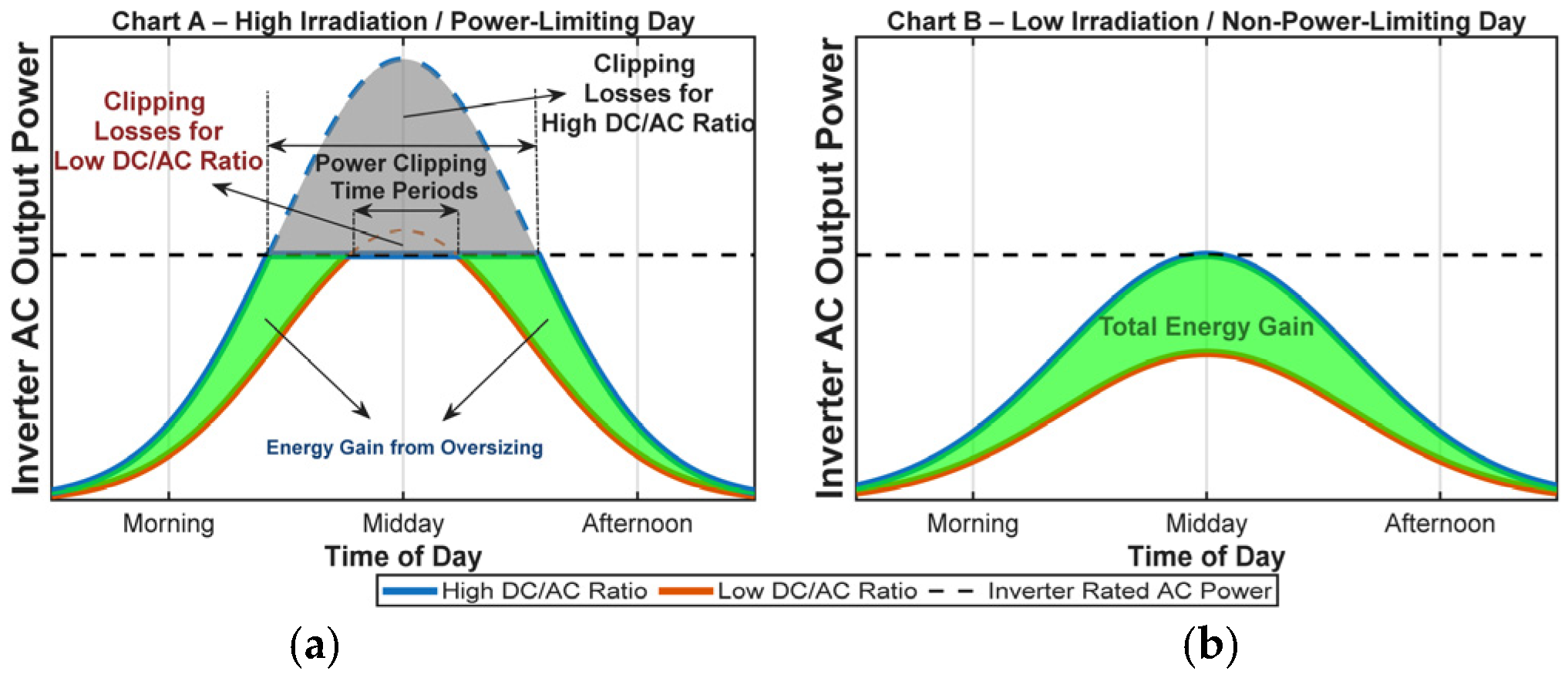
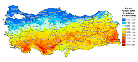
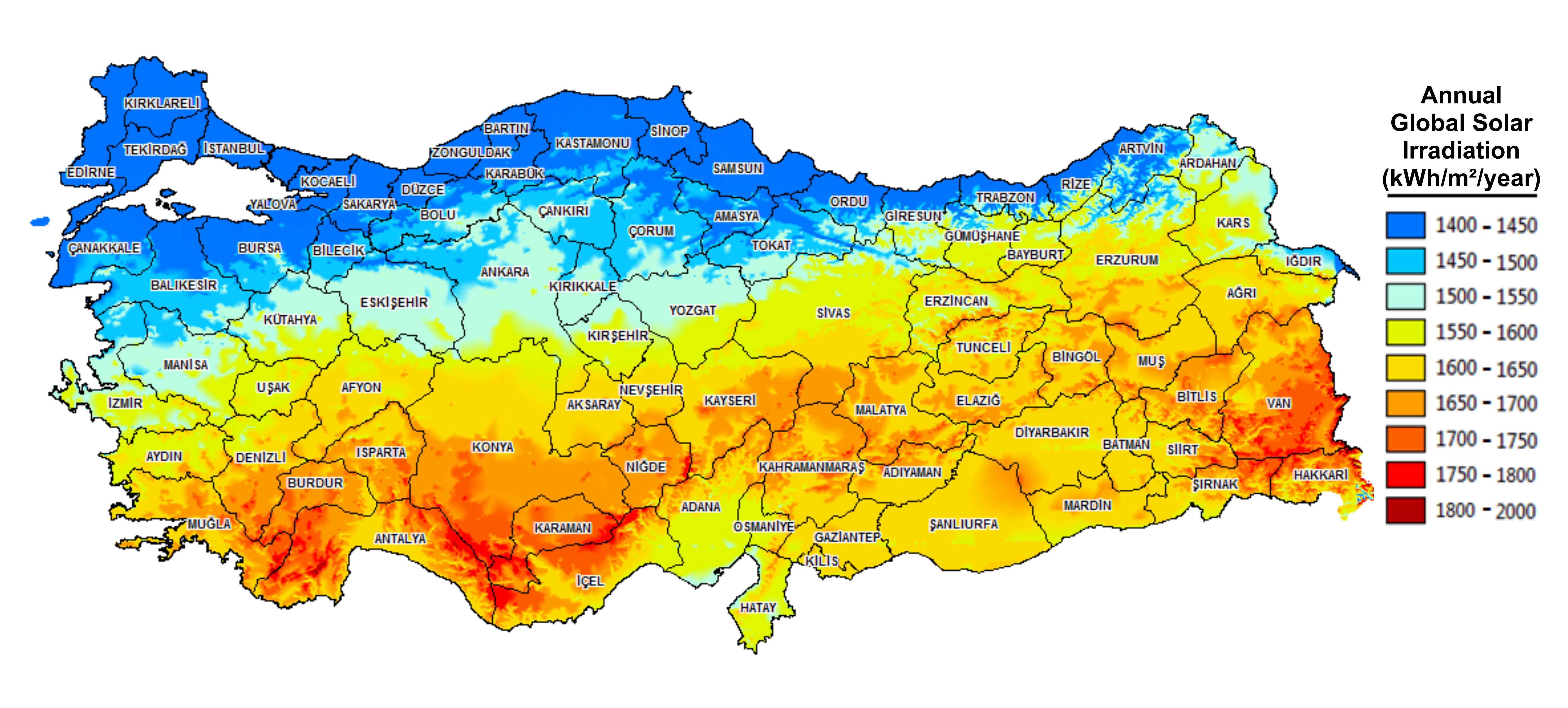
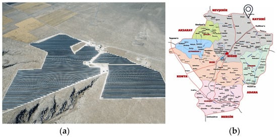
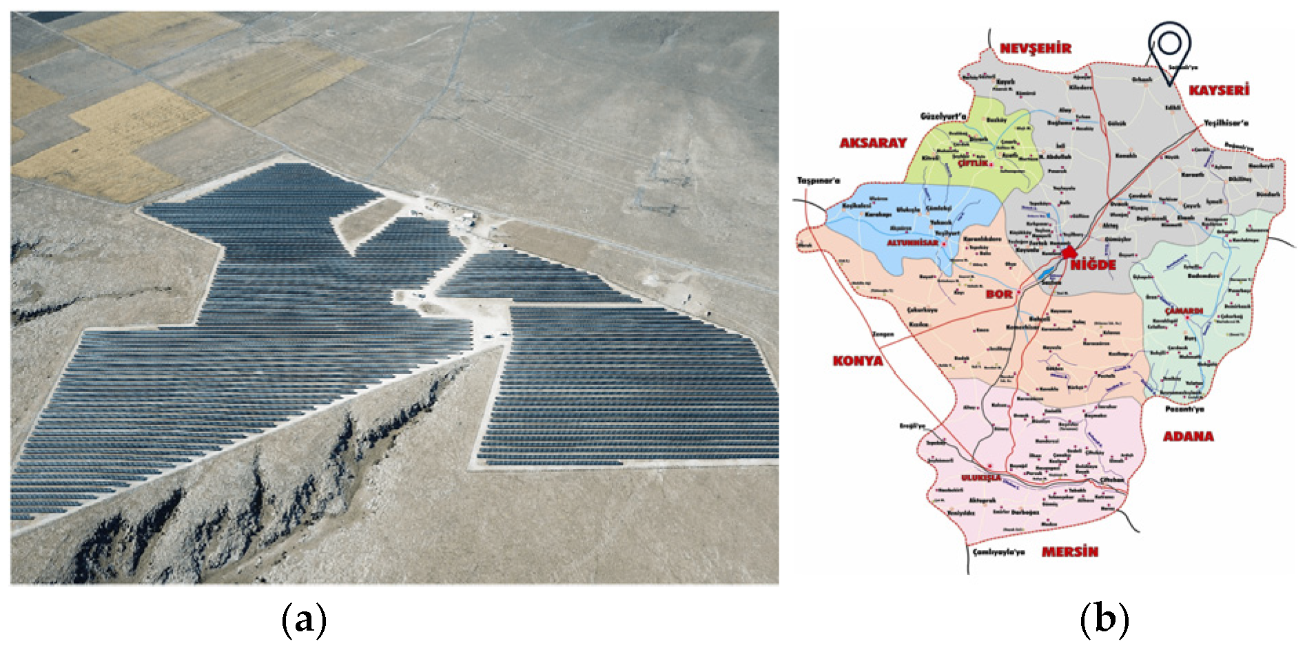


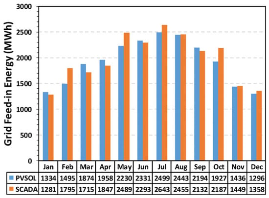
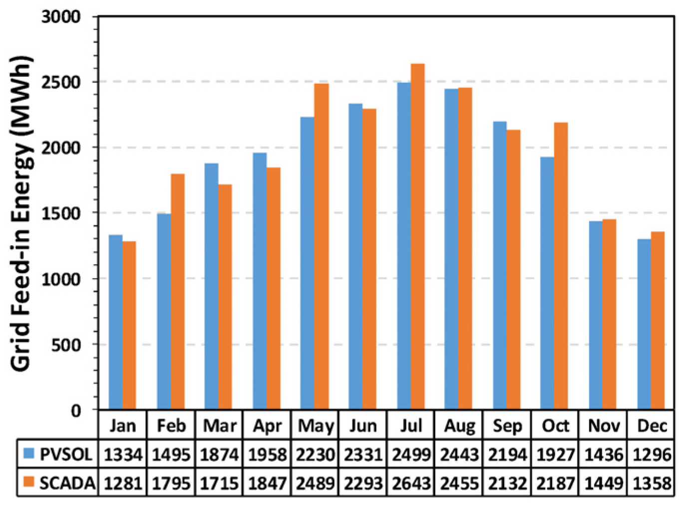
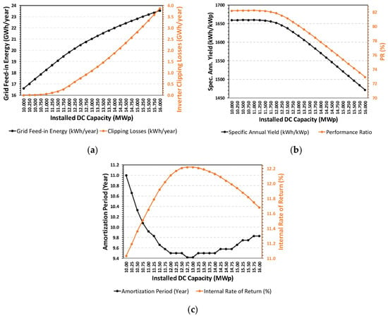
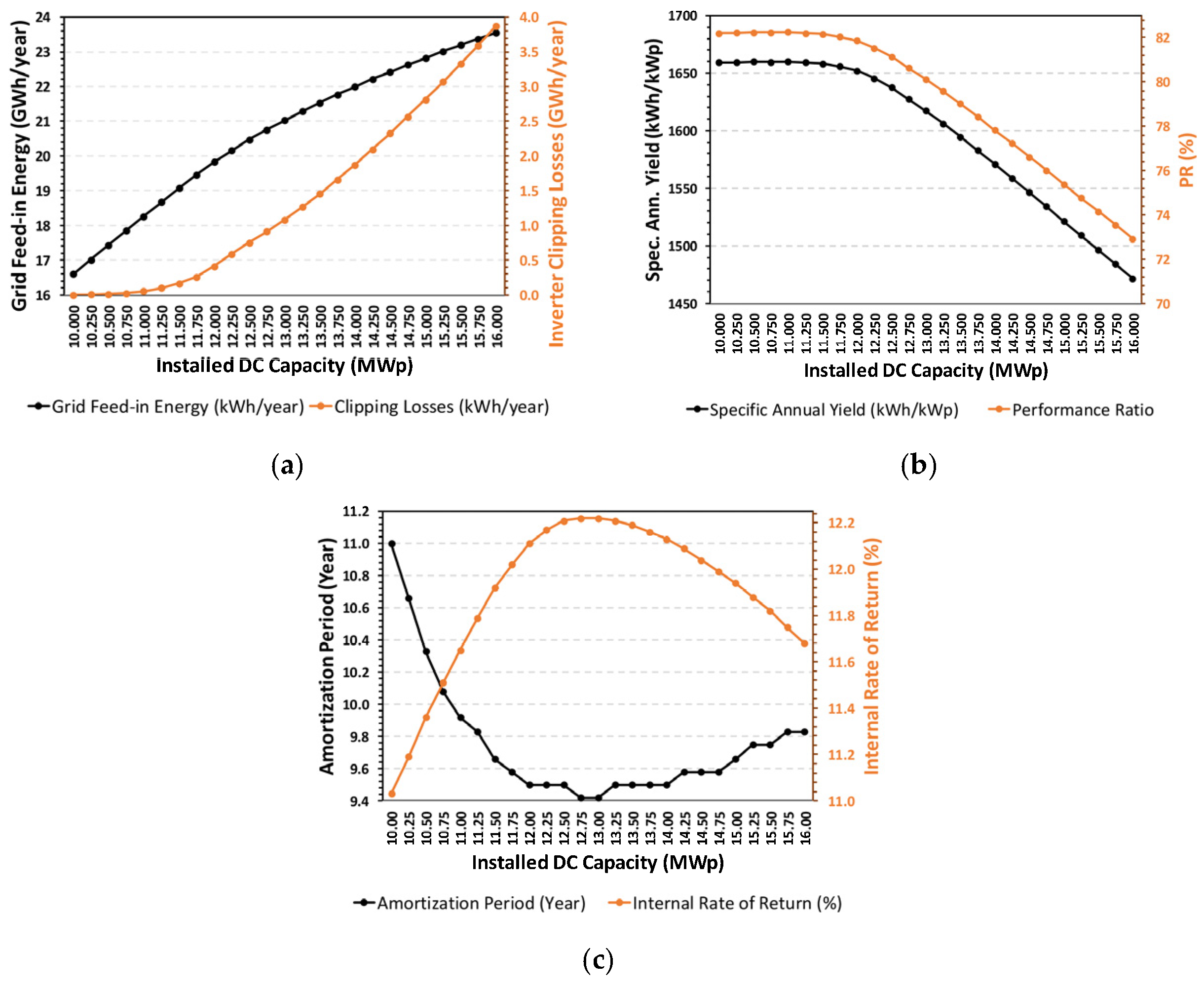

Disclaimer/Publisher’s Note: The statements, opinions and data contained in all publications are solely those of the individual author(s) and contributor(s) and not of MDPI and/or the editor(s). MDPI and/or the editor(s) disclaim responsibility for any injury to people or property resulting from any ideas, methods, instructions or products referred to in the content. |
© 2026 by the authors. Licensee MDPI, Basel, Switzerland. This article is an open access article distributed under the terms and conditions of the Creative Commons Attribution (CC BY) license.