


Abstract
Severe lost circulation in fractured shale formations limits the safe and efficient implementation of drilling operations, and the cuttings-migration behavior below the gas-injection point, which governs the cuttings-return performance of air-lift reverse circulation (ALRC) drilling, remains poorly quantified. To address this gap, this study develops a reduced-order liquid–solid model for cuttings migration below the gas-injection point, while the upper gas-lift zone is represented only through hydraulic pressure coupling. Agglomerated cuttings are treated as a continuous phase, the drill-pipe cross-section is discretized into radial layers to capture the radial velocity distribution of the liquid phase, and a quasi-steady spatial-marching algorithm with a local-equilibrium slip closure is adopted to simulate long-distance cuttings transport. Under the no-interlayer-exchange assumption, the model predicts strong near-wall cuttings retention during gas-free liquid–solid circulation. This result is interpreted as a conservative, model-dependent transport estimate rather than a direct prediction of permanent field-scale retention. In the Nr = 10 calculation, gas injection at 800 m above the bottom hole increases the predicted near-wall cuttings-migration height by approximately 13.8% relative to the gas-free case. For the composite reference case, gas-injection heights of 600, 700, and 800 m above the bottom hole are compared at a fixed gas flow rate of 0.100 m3 s−1. Among the three discrete heights tested at the finest investigated radial resolution, 600 m produced the largest fraction of inlet cuttings mass reaching the gas-injection interface. This result establishes only the relative ranking of the three tested cases and does not identify a continuously optimized or meter-scale gas-injection position. The 13.27 m difference between the Nr = 8 and Nr = 10 predictions is retained as an indicator of unresolved radial-resolution sensitivity.
1. Introduction
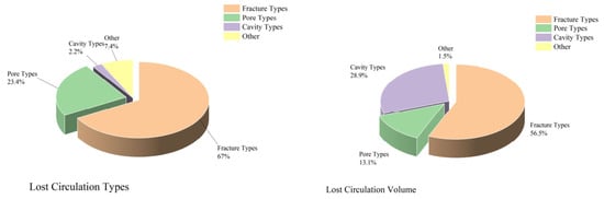
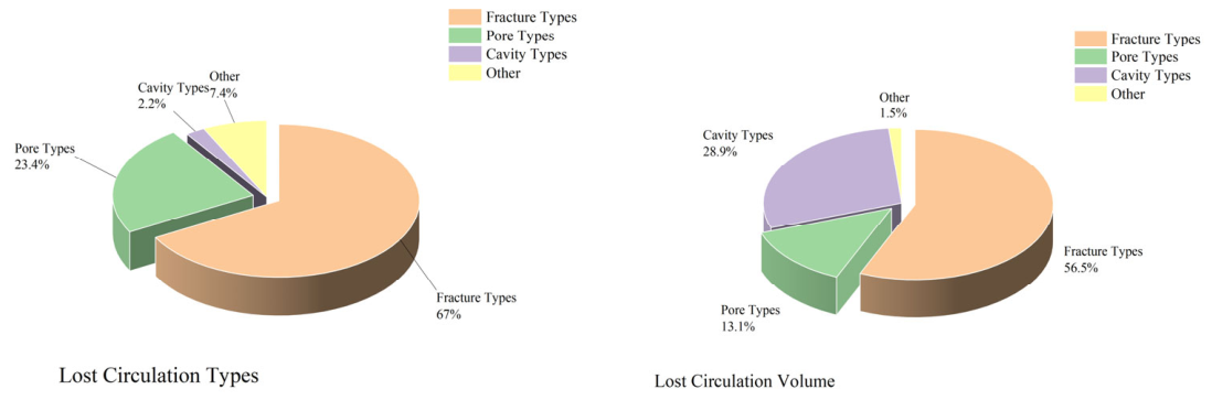
Severe lost circulation frequently affects shale-gas drilling and severely restricts operational safety and efficiency [1]. Statistical data from 162 vertical wells in X Block documented 337 leakage incidents with a total mud loss of 231,142.75 m3; 83.22% of the leakage volume (192,351.01 m3) occurred in the fractured Leikoupo, Jialingjiang, and Feixianguan Formations (Table 1, Figure 1). Fracture development is the primary cause of local leakage, and conventional positive-pressure drilling further activates fracture permeability, motivating the application of air-lift reverse circulation (ALRC) negative-pressure drilling to solve cuttings-transport issues. The mechanisms of drilling-fluid loss into fractured formations and the corresponding lost-circulation control strategies have been reviewed extensively in recent studies [2,3].
Table 1.
Summary of Leakage Situation in Region 1X.
Figure 1.
Types of leaks and the proportion of leaked quantity.
Traditional positive-pressure drilling faces high leakage risks in fractured-cavity shale formations and fails to meet field demands [4]. ALRC, a representative negative-pressure drilling technology, injects compressed air into the drill pipe–annulus gap to form low-density gas–liquid mixtures. The fluid density difference generates an upward lifting force, reducing wellbore circulation loss, suppressing bottom-hole overbalance, and mitigating formation leakage fundamentally [5,6,7].
Air-lift reverse circulation differs fundamentally from conventional air-reverse-circulation drilling [8]. The latter relies solely on compressed-air kinetic energy to carry cuttings, whereas ALRC creates buoyancy through the in-pipe density variation induced by gas injection. This study focuses on liquid–solid two-phase cuttings migration below the gas-injection point of ALRC wells.
Air-lift reverse circulation has been widely applied in oil–gas, geothermal, and geological drilling and in vertical slurry pumping [9,10], yet unstable cuttings discharge is frequently observed in field practice. Cuttings-return performance hinges on a matched gas-injection depth and flow rate; clarifying the in-pipe liquid–solid migration law is therefore critical to overcoming this engineering bottleneck.
Computational fluid dynamics (CFD) simulation, the primary tool for two-phase-flow research, includes Euler–Euler and Euler–Lagrange frameworks [11,12]. The Euler–Euler model is computationally efficient but ignores particle–particle and particle–wall collisions, which limits its precision. Coupling the Euler–Lagrange approach with the discrete element method (DEM) accurately captures particle dynamics, yet it adapts poorly to long drill strings and cannot directly support field parameter optimization [13,14]. CFD–DEM simulations of drill-pipe rotation and jet comminution have further revealed the complex particle–fluid interactions during cuttings transport [15,16].
Previous ALRC studies have developed whole-well pressure and lifting-force models to evaluate circulation feasibility and operating parameters. Chinese engineering studies have selected gas flow rate, liquid displacement, gas-injection depth, and dual-wall drill-pipe depth according to bottom-hole-pressure limits and safe operating windows [17,18]. Related reverse-circulation studies have also used critical carrying velocity, minimum gas supply, and pressure loss as quantitative design criteria [19,20]. Recent CFD–DEM studies have resolved local particle–fluid interactions and examined the effects of mud hydrodynamics, gas injection, submergence, viscosity, and drill-bit rotation [14,21]. Unified transient solid–liquid transport models, slurry-flow experiments, and CFD simulations provide additional foundations for cuttings-transport analysis [22,23,24]. However, these approaches do not directly predict layer-dependent cuttings stopping positions caused by radial variations in liquid carrying velocity below the gas-injection interface. The present study addresses this narrower local transport problem at a prescribed gas flow rate, rather than claiming universal or joint optimization of gas flow rate and injection height.
2. Materials and Methods
2.1. Physical Model Assumptions and Reference Frame
This section presents the physical model, the governing equations, the numerical solution procedure, and the boundary conditions for the bottom-hole region below the gas-injection point. The definitions of the flow parameters used in the derivations are collected in Appendix A for completeness.
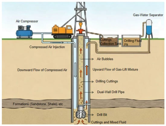
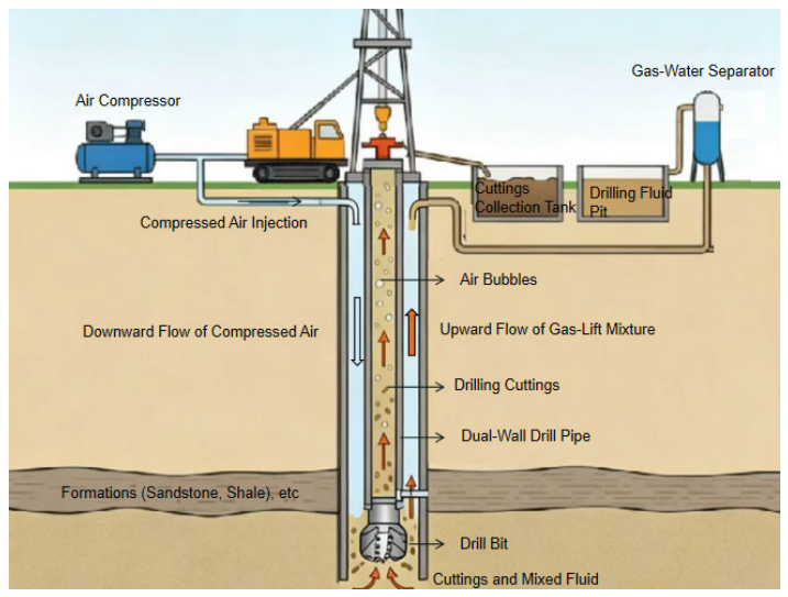
The air-lift reverse circulation (ALRC) system consists of wellhead equipment, dual-wall drill pipe, drill bit, air-injection unit, and ground circulation facility (Figure 2). Drilling fluid flows downward through the drill pipe–formation annulus to the bottom hole, carrying cuttings into the drill-pipe inner cavity to form a liquid–solid two-phase flow. Below the gas-injection interface, the model solves the liquid–solid two-phase transport problem. At zg, the prescribed gas flow enters a simplified hydraulic representation of the upper gas-lift zone. Only its pressure effect is transmitted to the lower liquid–solid model; axial cuttings transport above the interface is not solved.
Figure 2.
Schematic diagram of the gas-lift reverse-circulation drilling system.
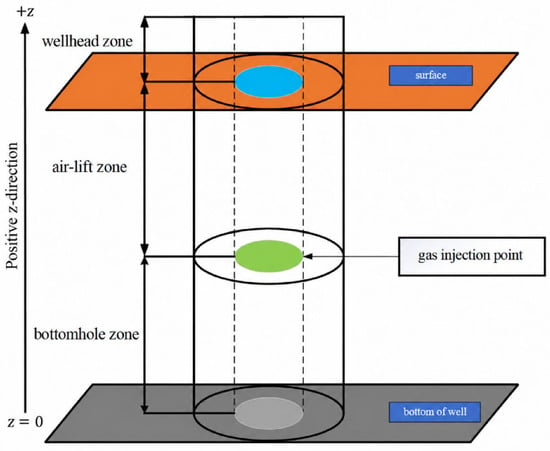
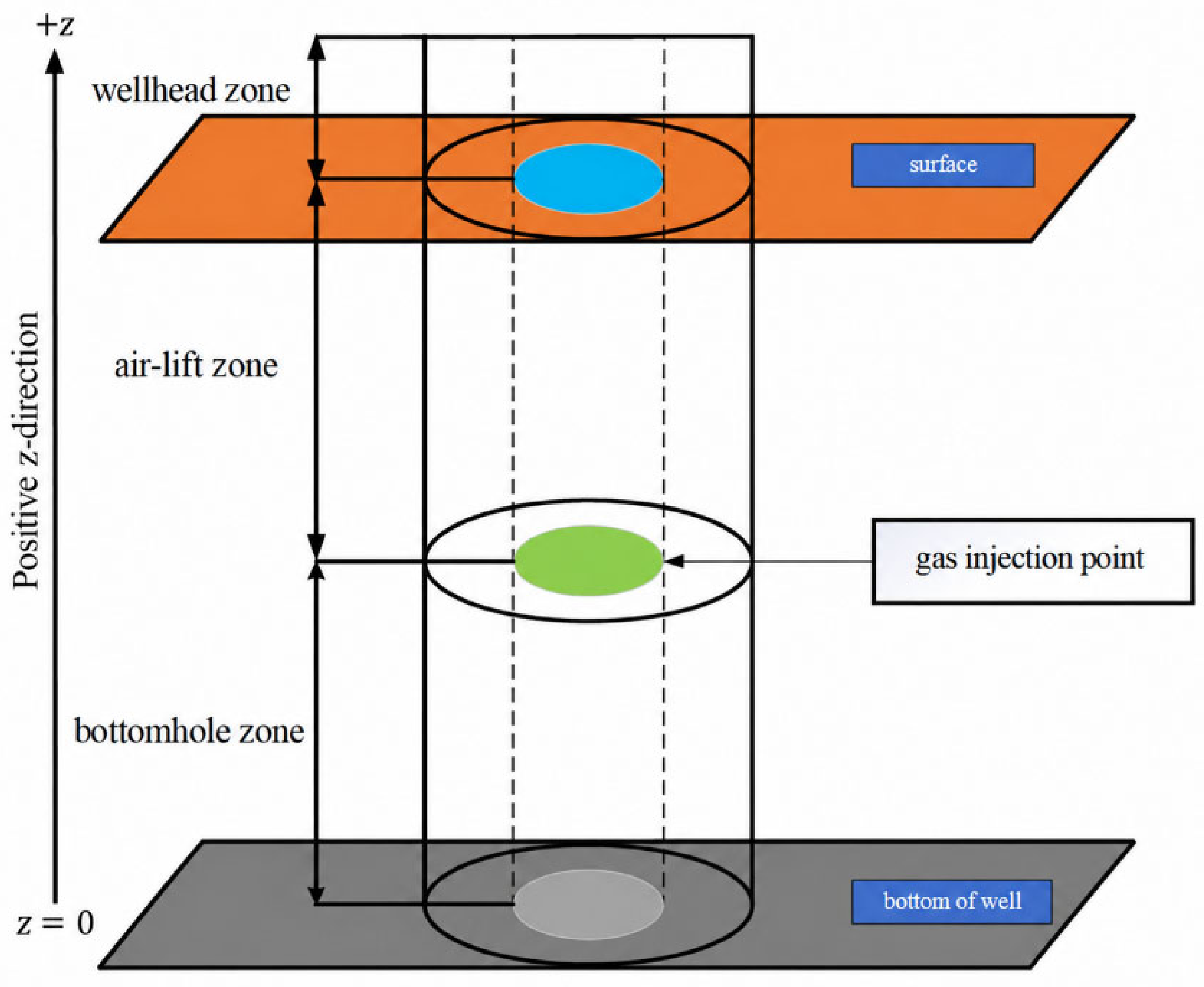
Based on the flow features, the wellbore is divided into three zones: a liquid–solid two-phase bottom-hole zone below the gas-injection point, a gas–liquid–solid three-phase lift zone up to the wellhead, and a surface separation zone (Figure 3). This study concentrates on cuttings migration in the bottom-hole two-phase region. Figure 3 defines the coordinate systems used throughout this study. The axial model coordinate z is measured upward from the bottom hole, whereas the field measured depth MD is measured downward from the wellhead. Accordingly, the gas-injection position is reported primarily as the height zg above the bottom hole.
Figure 3.
Air-lift reverse-circulation partition.
The model is developed for upward cuttings transport in the internal return passage of a straight vertical drill pipe. The following assumptions are adopted: (1) the drilling fluid is incompressible; (2) the inlet solid volume fraction is below 5%, and the cuttings are represented as a dilute continuous dispersed phase; (3) the cuttings are represented by equivalent spherical particles of uniform diameter and are initially distributed uniformly across the inlet; (4) the drill pipe is stationary, with no rotational or orbital motion; (5) the return passage is circular, axisymmetric, and of constant diameter; (6) finite particle relaxation and the entrance-acceleration region immediately above the bit are not resolved. The reduced-order model is quasi-steady and employs a local-equilibrium algebraic-slip closure in every axial cell. Neither the local nor the convective acceleration of the cuttings phase is solved. Axial variations in the calculated cuttings velocity therefore represent a sequence of local-equilibrium states rather than a resolved particle-acceleration process. (7) The radial layers are treated as uncoupled axial transport paths. Radial cuttings-mass exchange, interlayer momentum transfer, turbulent particle dispersion, collision-induced radial migration, and re-entrainment from the near-wall region are not resolved.
Accordingly, the reported predictions apply to dilute, upward, turbulent liquid–solid flow below the gas-injection point in a straight vertical circular return passage. For the cases considered here, the inlet solid volume fraction is below 0.05, the particle diameter is 0.005 m, the drill-pipe diameter is 0.127 m, and the drilling-fluid flow rate is 12 L s−1. The imposed gas-injection flow rates are 0 and 100 L s−1, and the investigated injection depths range from 600 to 800 m, as summarized in Table 2. Extrapolation to concentrated slurries, broad or strongly nonspherical particle populations, inclined or horizontal wells, eccentric annuli, rotating drill pipes, or start-up and pulsating flows requires separate validation.
Table 2.
Basic parameters of the calculation example.
The effects of these assumptions cannot be represented by a single universal error percentage because dedicated sensitivity simulations were not performed for compressibility, inlet nonuniformity, particle shape, or drill-pipe rotation. Previous CFD–DEM results indicate that the magnitude of the rotation effect is strongly condition-dependent. The cited CFD–DEM study reported little change in cuttings concentration when the rotation rate increased from 0 to 80 rpm at low inlet velocity, but a marked improvement when it increased from 100 to 120 rpm; at high inlet velocity, the rotation effect was nearly negligible. Because that study considered a horizontal annulus, its numerical results cannot be transferred directly to the present vertical internal return passage. The stationary-pipe predictions should therefore be interpreted as a baseline that may underpredict rotation-enhanced cuttings removal under low-to-moderate carrying velocities. The predicted critical migration heights for Nr = 5), 8, and 10 are 735.09, 756.88, and 770.15 m, respectively. The Nr = 8 and Nr = 10 predictions differ by 13.27 m, or 1.75% relative to the 8-layer result. Although this percentage is small relative to the total migration distance, the corresponding absolute difference is not negligible for meter-scale engineering decisions. It is therefore treated as unresolved radial-resolution sensitivity rather than as evidence of grid independence. The Nr = 10 result is used only as the finest tested reference calculation.
A one-dimensional Eulerian reference frame fixed to the drill pipe is adopted. The origin is located at the bottom hole, and the positive z-direction points vertically upward. The liquid-phase velocity vl is the upward axial liquid carrying velocity measured relative to the drill pipe, wh is the positive downward hindered-settling velocity of the cuttings relative to the liquid, and vs is the net absolute axial velocity of the cuttings in the pipe-fixed reference frame. Under the local-equilibrium algebraic-slip approximation, these velocities satisfy vs = vl − wh. Therefore, the cuttings migrate upward when vl > wh, whereas the maximum migration height is reached when vl = wh, equivalently vs = 0. Gravity acts in the negative z-direction. The Eulerian flow field is treated as quasi-steady. The time reported for cuttings migration is the accumulated Lagrangian travel time of the cuttings and is not the transient time of the Eulerian flow field.
2.2. General Balance Equations and Reduced-Order Model
The phase-averaged governing equations are formulated in the pipe-fixed Eulerian reference frame. Here, Ck, ρk, and vk denote the volume fraction, density, and axial velocity of phase k, respectively, where k = l denotes the liquid phase and k = s denotes the solid phase. The drill-pipe cross-sectional area is denoted by A, and Cl + Cs = 1.
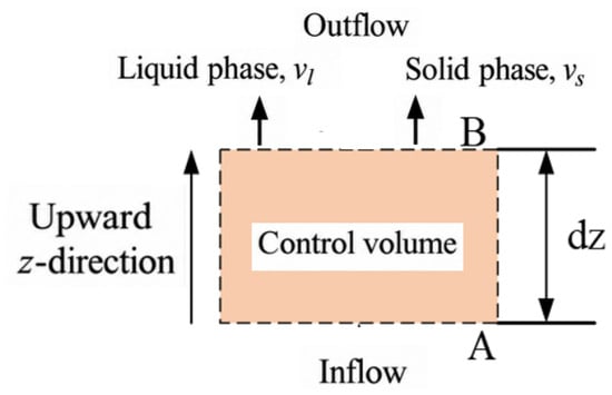
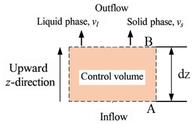
The liquid and solid phases are treated as interpenetrating continua in a pipe-fixed Eulerian reference frame. The corresponding phase-averaged mass and momentum balances follow the classical two-fluid formulation, while recent reverse-circulation cuttings-transport studies are cited as application-specific precedents. The phase fractions, axial velocities, pressure gradient, interphase momentum exchange, and wall-force densities acting within the differential control volume are illustrated in Figure 4.
Figure 4.
Differential control volume and sign conventions for the one-dimensional liquid–solid two-phase flow model.
For completeness, the general phase-averaged mass and momentum balances are presented below to define the force terms and sign conventions. These momentum equations are not integrated in the reduced-order calculation.
Therefore, the axial mass flux of each phase remains constant. In the calculation used in this study, the liquid velocity is obtained from the pressure-loss and radial-velocity-profile closures, whereas the cuttings velocity is obtained algebraically from the local-equilibrium slip closure in Section 2.2.2. Accordingly, neither the local nor the convective acceleration of the cuttings phase is resolved.
In Equations (3) and (4), Ms is the interphase momentum-transfer force acting on the solid phase per unit mixture volume. The corresponding force acting on the liquid phase is −Ms, in accordance with Newton’s third law. The quantities fwl and fws are the signed wall-interaction force densities acting on the liquid and solid phases, respectively. A positive force is defined as acting in the upward z−direction.
The interphase forces cancel when the two phase-momentum equations are summed. The pressure-gradient force is weighted by the corresponding phase volume fraction in Equations (3) and (4). Because the pressure-gradient and gravitational terms are already included explicitly, particle buoyancy is not introduced as an additional independent force. This convention avoids double counting. The lifting force defined later for the gas-lift zone represents the macroscopic hydrostatic driving force between the annular liquid column and the internal gas–liquid column and should not be confused with particle buoyancy in the bottom-hole region.
2.2.1. Interphase Momentum Transfer
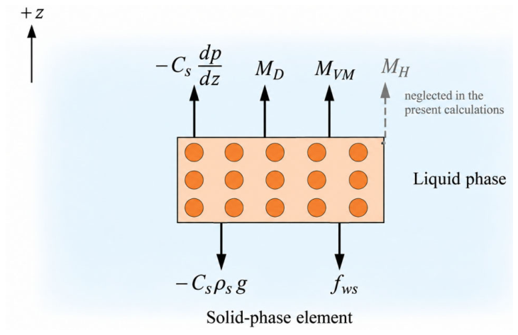
The interphase momentum transfer acting on the solid phase is decomposed into drag and history-force contributions, which are commonly identified in the equation of motion of a particle in a nonuniform flow:
Fe = Fd + Fba
Here, MD, MVM, and MH are volumetric force densities rather than forces acting on an individual particle; therefore, each term has dimensions of N M−3.
The directions and sign conventions of the force-density terms acting on the solid phase are shown in Figure 5. The pressure-gradient and gravitational terms are written explicitly in the solid-phase momentum equation, whereas drag and history effects are included through the interphase momentum-transfer term.
Figure 5.
Calculation unit force diagram.
Here, CD is the particle drag coefficient, dp is the particle diameter, and the sign of vl − vs determines the direction of the drag acting on the solid phase. The particle Reynolds number is calculated as follows:
The characteristic particle Reynolds number is approximately Rep = 2.45 × 10³ under the representative operating conditions. This value lies outside the creeping-flow regime underlying the classical Basset history-force kernel. Therefore, the classical Basset expression is not used in the present reduced-order model, and MH = 0 is adopted as a modelling approximation rather than as a general consequence of the high particle Reynolds number. The possible influence of unsteady-history effects, particularly during gas-injection start-up, is not resolved and is regarded as a limitation of the present formulation.
2.2.2. Local-Equilibrium Velocity Closure
The general momentum equations presented above are not integrated in the reduced-order calculation. Instead, the model assumes that the cuttings attain the local hindered-settling slip velocity within each axial cell. The net absolute axial velocity of the cuttings is therefore evaluated algebraically as
where wh is the hindered-settling velocity relative to the liquid and is defined as positive downward. Although vl, wh, and vs may vary with axial position, this variation represents successive local-equilibrium states rather than resolved solid-phase acceleration.
vs = vl − wh
The liquid–solid relative velocity is as follows:
ur = vl − vs = wh
vs > 0: upward migration; vs ≤ 0: stopping condition
The cuttings migrate upward when vs > 0. The first axial location at which vs ≤ 0, equivalently vl ≤ wh, is recorded as the maximum cuttings-migration height.
When the net cuttings velocities at two adjacent axial nodes are both positive, the Lagrangian travel time is evaluated using the average net solid-phase velocity:
where Δzi is the axial-cell length, and tp,i,j and tp,i+1,j are the accumulated Lagrangian travel times at two adjacent axial nodes. Equation (13) is applied only when the net cuttings velocities at both nodes are positive. It is used solely to accumulate the Lagrangian travel time and is not an Eulerian transient equation. It does not feed back into the algebraic velocity closure. If vs ≤ 0 is obtained in an axial cell, the travel-time update is terminated and the corresponding axial position is recorded as the maximum cuttings-migration height.
2.3. Pressure-Loss and Radial Liquid-Velocity-Profile Closures
In the present calculations, the cross-section-averaged inlet solid volume fraction is below 5%; the bottom-hole region is therefore treated as a dilute turbulent liquid–solid pipe flow. This global criterion does not guarantee that every near-wall computational cell remains dilute after local accumulation. The frictional pressure-loss gradient is evaluated using the Darcy–Weisbach formulation, with the friction factor obtained from the Colebrook correlation [24]. For upward flow in the positive z−direction, the frictional pressure gradient is negative; therefore, its positive loss magnitude is written as follows:
where fD is the Darcy friction factor and D is the internal diameter of the drill pipe.
In fully developed turbulent pipe flow, the axial liquid-phase velocity varies with radial position. It reaches its maximum at the pipe center and decreases toward the pipe wall. This variation represents the radial profile of the axial liquid-phase carrying velocity rather than a radial velocity component and is expressed as follows:
where Rp is the internal radius of the drill pipe and kv is the velocity-profile shape parameter.
The value of vl,max is determined so that the cross-sectional average of vl(r) is equal to the prescribed average liquid-phase velocity.
The decrease in the liquid-phase carrying velocity near the pipe wall increases the likelihood of cuttings retention. The drill-pipe cross-section is therefore divided into radial layers to resolve the radial variation of vl(r) and the resulting variation in the net cuttings velocity vs. In addition, particle settling in a confined conduit is affected by the particle-to-pipe blockage ratio [25].
The net upward velocity of the cuttings depends on both the local liquid-phase carrying velocity and the settling velocity relative to the liquid. At finite solid concentrations, hydrodynamic interactions between particles reduce the settling velocity relative to that of an isolated particle. The local hindered-settling velocity is evaluated using the Richardson–Zaki relation [26,27,28]:
Here, wt0,i,j is the local terminal settling velocity of an isolated particle relative to the liquid, Cs,i,j is the local cuttings volume fraction, nRZ is the Richardson–Zaki exponent, and wh,i,j is the local positive downward hindered-settling velocity relative to the liquid.
The Richardson–Zaki relation is applied uniformly to all computational cells. Cells with Cs ≤ 0.03 are treated within the dilute-suspension range. Cells with Cs > 0.03 use the same closure, but their predictions are regarded as less reliable because particle contacts, clustering, and granular stresses are not explicitly resolved. The exponent nRZ is fixed according to the particle-settling regime represented by the cited Richardson–Zaki correlations and is not varied between axial cells.
The settling velocities wt,0 and wh are relative velocities, whereas vl(r) is the local absolute liquid-phase carrying velocity and vs is the net absolute cuttings velocity in the pipe-fixed frame. According to Equation (12), the cuttings migrate upward when vs > 0. The maximum migration height is reached when vs ≤ 0, equivalently vl ≤ wh.
2.4. Hydraulic Coupling with the Gas-Lift Zone
This study solves liquid–solid cuttings transport only below the gas-injection point. The upper gas-lift zone is represented by simplified mixture-density and pressure-loss relations that provide the interface pressure for the lower-region calculation. Related airlift behavior has been characterized experimentally in previous studies [29,30].
The liquid–solid flow in the lift zone mixes with injected air to form a three-phase flow. Since cuttings occupy a tiny volume fraction, the mixture density is dominated by gas–liquid proportions, with the corresponding formula given below:
ρgl = εgρg + εlρl
The change of pressure and temperature along the wellbore will directly change the value of gas-phase density. The ideal-gas state equation is used to solve for the gas density at different well depths. This assumption is restricted to the prescribed pressure and temperature range of the reference case and is not intended to represent strongly non-ideal high-pressure gas behavior.
where Mg is the molar mass of the injected gas and Ru is the universal gas constant.
In the upper gas-lift zone, the density difference between the annular liquid column and the internal gas–liquid–solid mixture generates a macroscopic lifting force. This lifting force is distinct from the particle-scale buoyancy contribution already contained in the pressure-gradient and gravitational terms of the bottom-hole two-phase momentum equations.
Flift = (ρl − ρgl)gΩ
The gas-injection point is the common interface between the bottom-hole liquid–solid two-phase zone and the upper three-phase gas-lift zone. In order to ensure the self-consistency of the physical quantities of the whole wellbore flow field, two sets of continuity constraints are set at the interface:
At the gas-injection point, the static pressure at the outlet of the bottom-hole zone equals that at the inlet of the gas-lift zone, which gives:
pbottom(zg) = plift(zg)
In addition, the axial migration velocity of cuttings is continuous across the interface between the two zones, which gives:
The present cuttings-transport calculation terminates at the gas-injection interface. The upper gas–liquid–solid section is represented only through simplified hydraulic relations for pressure coupling; axial cuttings transport from the interface to the wellhead is not solved.
The gas-injection height determines the lengths of the lower liquid–solid region and the upper gas-lift region and therefore affects the pressure distribution. The bottom-hole absolute pressure is obtained by integrating the pressure gradient downward from the gas-injection interface:
2.5. Numerical Discretization and Solution Procedure
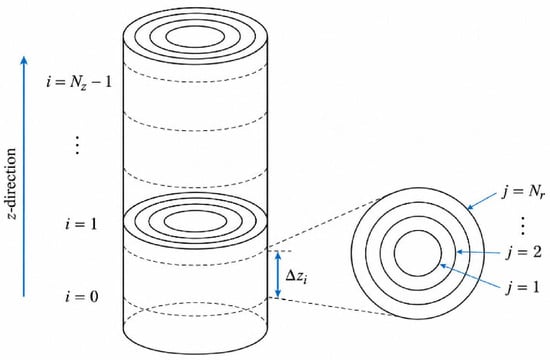
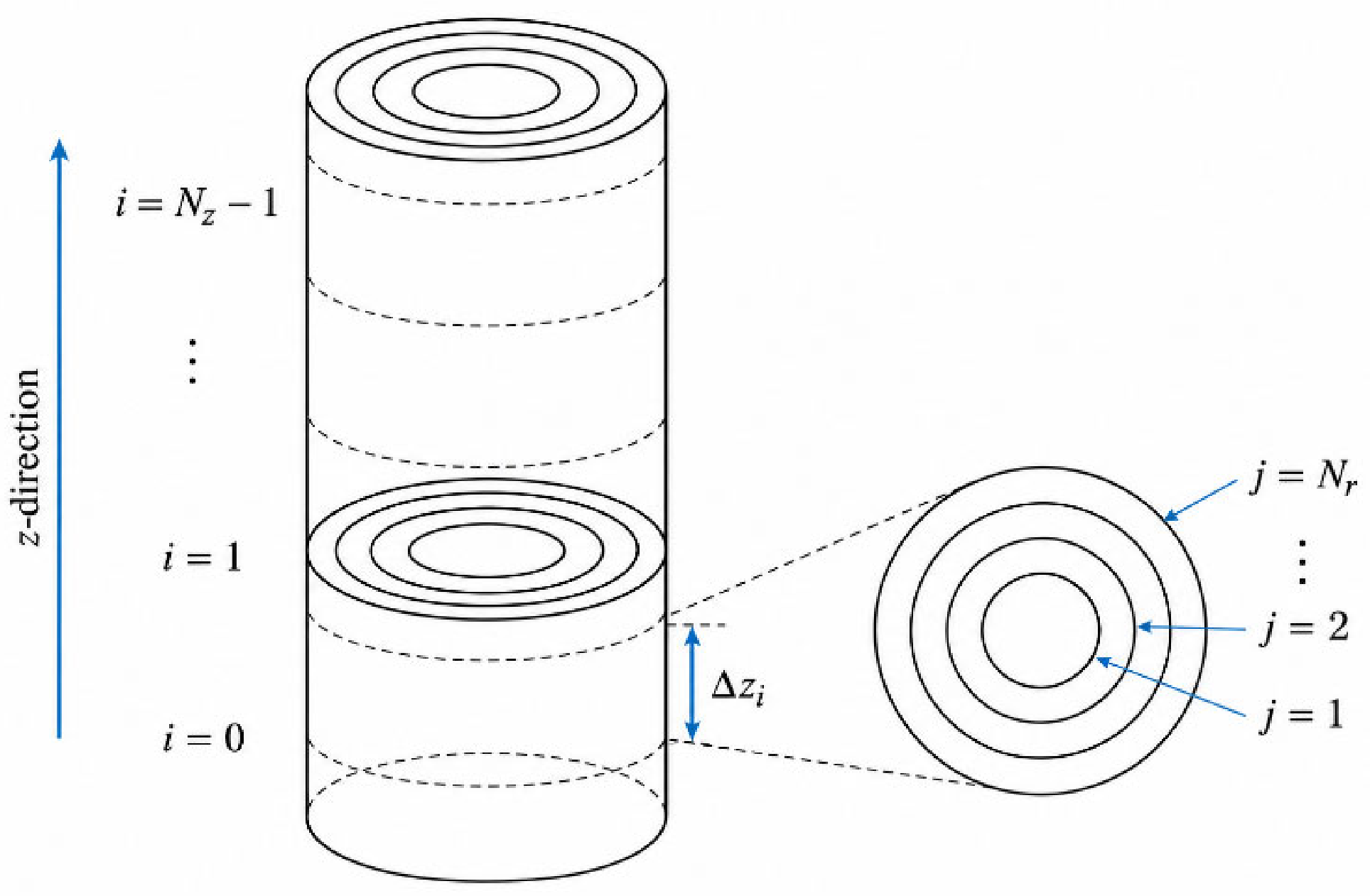
The bottom-hole drill-pipe domain is discretized into Nz axial cells indexed by i = 0,1,…,Nz − 1 and Nr radial layers indexed by j = 1,2,…,Nr. The axial coordinate z and radial coordinate r are Eulerian spatial variables. The calculation advances directly from axial cell i to axial cell i + 1, and no Eulerian time-step index is introduced. The variable tp denotes only the accumulated Lagrangian travel time of the cuttings.
The cases with Nr = 5, 8, and 10 were selected as coarse, intermediate, and fine radial resolutions for a screening grid-sensitivity analysis.
The axial and radial discretization of the liquid–solid flow domain is shown in Figure 6.
Figure 6.
Axial-cell and radial-layer discretization of the bottom-hole liquid–solid flow domain. The vertical ellipsis (⋮) indicates that the intermediate axial cells (from i = 2 to i = Nz − 2) are omitted for conciseness.
Using a prescribed spatial discretization, the length of axial cell i is defined as follows:
Δzi = zi+1 − zi
For a uniform axial grid, Δzi = Lb/Nz. The Lagrangian travel time is subsequently updated using Equation (13) and is not used to define the spatial grid.
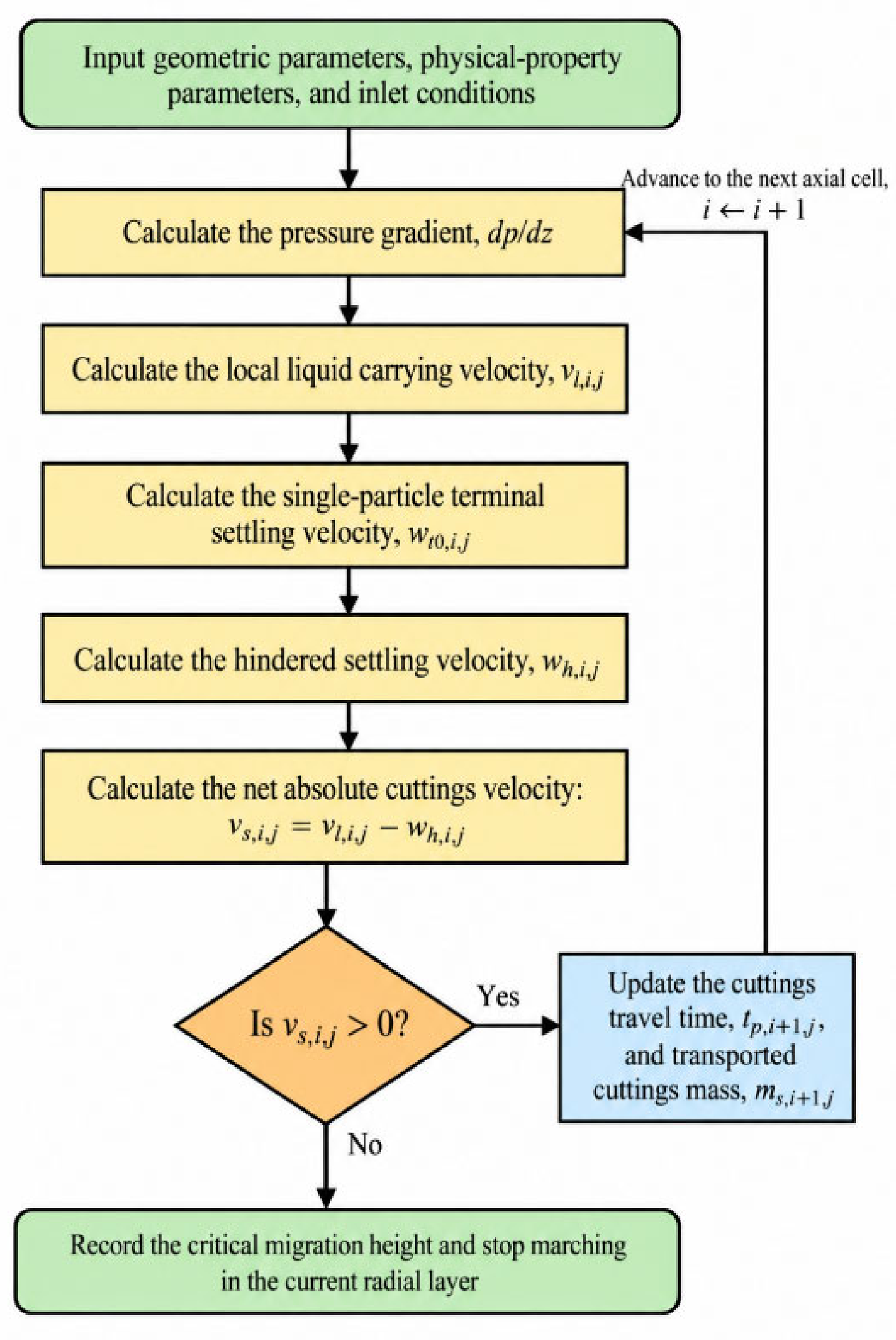
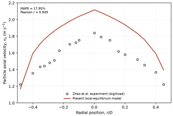
At each axial cell i and radial layer j, the local liquid-phase carrying velocity vl,i,j is first calculated from the pressure-loss and radial-velocity-profile closures. The single-particle terminal settling velocity wt0,i,j and the hindered-settling velocity wh,i,j are then evaluated from the local particle and slurry properties. Under the local-equilibrium algebraic-slip approximation, the net absolute cuttings velocity is calculated as vs,i,j = vl,i,j − wh,i,j. When vs,i,j > 0, the cuttings continue to migrate upward, and the Lagrangian travel time and transported cuttings mass are updated. When vs,i,j ≤ 0, the current axial position is recorded as the maximum migration height for radial layer j.
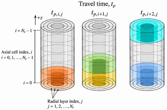
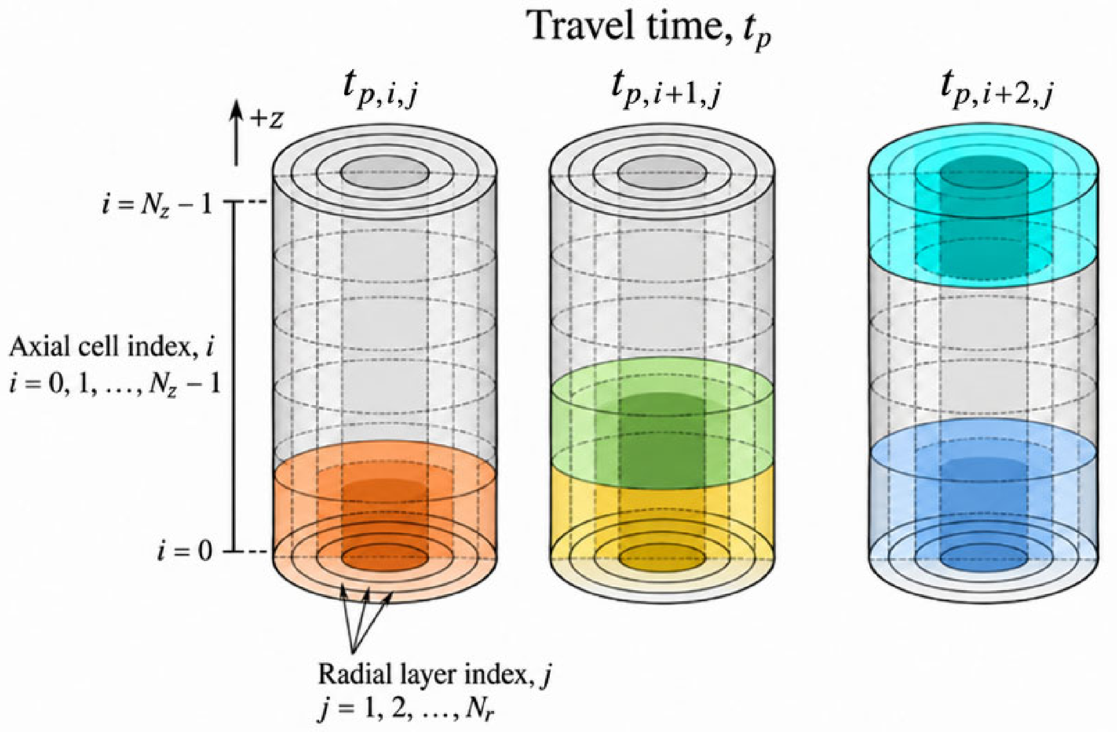
Figure 7 schematically illustrates the sequential axial migration of the cuttings and the accumulation of the Lagrangian travel time tp within the discretized domain.
Figure 7.
Axial-cell and radial-layer indexing used to track the Lagrangian travel time of cuttings. In each schematic, the upper colored cell indicates the current cuttings position at the specified travel time, whereas the lower colored cells indicate previously traversed axial cells. The colors are used only to distinguish the illustrated migration steps and do not represent physical quantities.
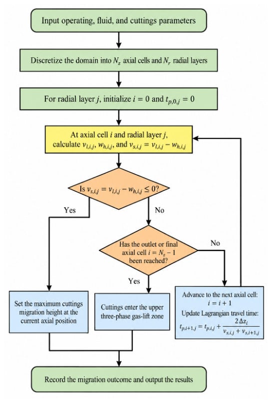
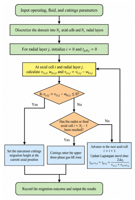
The calculation for radial layer j terminates when either (i) the cuttings reach the gas-injection interface with vs,i,j > 0, in which case they enter the upper three-phase gas-lift zone, or (ii) vs,i,j ≤ 0 before the interface is reached, in which case the current axial position is recorded as the maximum cuttings-migration height.
The quasi-steady spatial-marching logic and the stopping criterion used to determine the maximum cuttings-migration height are summarized in Figure 8.
Figure 8.
Quasi-steady spatial-marching procedure for determining the maximum cuttings-migration height.
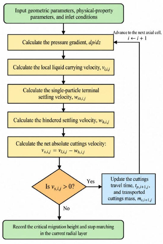
The complete local calculation sequence is summarized in Figure 9. After the geometric parameters, physical properties, and inlet conditions are specified, the pressure gradient and the local liquid-phase carrying velocity vl,i,j are calculated. The single-particle terminal settling velocity wt0,i,j is then corrected for the local solid concentration to obtain the hindered-settling velocity wh,i,j, and the net cuttings velocity is evaluated as vs,i,j = vl,i,j − wh,i,j. If vs,i,j > 0, the Lagrangian travel time tp and the transported cuttings mass are updated, and the calculation advances to the next axial cell. Otherwise, the critical migration height is recorded and the calculation for the current radial layer is terminated. Throughout this study, “stopping” denotes the termination of axial marching for an individual radial layer when its calculated net cuttings velocity becomes non-positive.
Figure 9.
Calculation sequence for the net cuttings velocity and critical migration height in each radial layer.
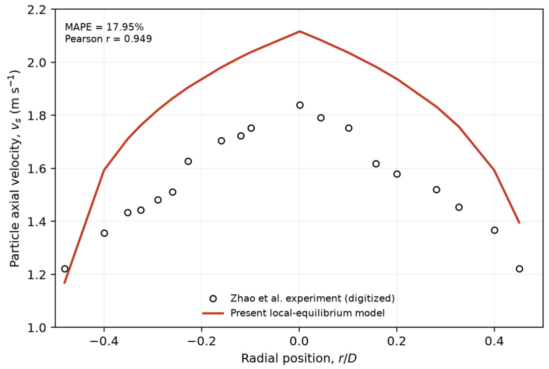
The present study distinguishes numerical verification from physical validation. Numerical verification covers dimensional consistency, stopping-criterion consistency, and radial-resolution comparison. Independent component-level validation used the measurements of Zhao et al. [31]. Nineteen velocity points were digitized from their Figure 11 of Zhao et al. without recalibrating the model coefficients.
2.6. Boundary Conditions
The boundary conditions are specified separately at the bottom-hole inlet, the gas-injection interface, and the drill-pipe wall.
2.6.1. Inlet Boundary
At the bottom-hole inlet z = 0, the cuttings mass entering during a prescribed material-injection interval Δtin is distributed among the radial layers in proportion to their cross-sectional areas. Thus,
Here, is the cross-sectional area of radial layer j, A = πR2 is the total pipe-flow area, and Δtin is used only to define a material parcel rather than an Eulerian numerical time step. For equal-area radial layers, Aj/A = 1/Nr.
The number of particles in the inlet parcel is np,(0,i,j):
The inlet solid and liquid volume fractions in radial layer j are calculated as follows:
At the inlet, the retention ratio is defined for vs,0,j > 0 as follows:
Here, Cs,A,0 denotes the cross-sectionally averaged inlet solid volume fraction. Equation (27) is evaluated only when vs,0,j > 0 and is not used at the stopping location where vs = 0.
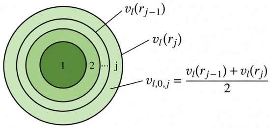
The radial discretization used to assign the inlet liquid velocity is shown in Figure 10. For radial layer j, the representative liquid-phase carrying velocity is approximated by the arithmetic mean of the velocities at the inner and outer boundaries, rj−1 and rj, respectively.
Figure 10.
Radial-layer discretization used to determine the representative inlet liquid-phase carrying velocity.
Liquid-phase flow, that is, drilling-fluid displacement, is a known term:
Ql(z = 0) = Ql,in
Liquid-phase velocity distribution can be estimated as follows:
Consistent with the local-equilibrium algebraic-slip approximation, the inlet net cuttings velocity is determined from the following:
vs,0,j = vl,0,j − wh,0,j
In the process of gas-lift reverse circulation, the inlet pressure is the formation pressure, which is also known, as shown in the formula:
p(z = 0) = pb
2.6.2. Outlet Boundary
The outlet of the bottom-hole region is located at the gas-injection interface z = Lb. If the cuttings in radial layer j reach this interface with vs,i,j > 0, they are recorded as reaching the gas-injection interface. If vs,i,j ≤ 0 before the interface is reached, the corresponding axial position is recorded as the maximum cuttings-migration height for that radial layer.
Here, istop,j denotes the last completed axial cell in radial layer j. Because Δzi has dimensions of length, Equation (32) also has dimensions of length.
2.6.3. Wall Boundary
The wall-interaction force is treated separately from the liquid–solid interphase force. For a circular drill pipe, the signed solid–wall force per unit mixture volume is written as follows:
Here, Pw = πD is the wetted perimeter, A = πD2/4 is the pipe cross-sectional area, D is the internal diameter, and τw,s is the magnitude of the solid–wall shear stress. Therefore, fw,s has units of N m−3, and its direction is opposite to the net cuttings velocity vs.
3. Results and Discussion
Based on the model and solution procedure presented in Section 2, a composite reference case was constructed using representative parameters reported for several shale-gas fields in the Sichuan Basin. The input set does not represent a single field well. Drilling-fluid properties were taken from the Nanchuan block, cuttings properties from the Changning field, drilling-fluid flow rate and rate of penetration from the Fuling field, and borehole and drill-pipe dimensions from the Pingye 1 well group. Prescribed numerical parameters were added to define the comparative simulations.
The compatibility of the composite input set was checked before the comparative simulations. The prescribed borehole diameter and rate of penetration give a cuttings-generation rate of approximately 1.42 × 10⁻⁴ m3 s−1. Together with a drilling-fluid flow rate of 0.012 m3 s−1, this corresponds to an inlet cuttings volume fraction of approximately 1.17%, which is consistent with the dilute-flow assumption. The mean liquid velocity in the 0.127 m internal return passage is approximately 0.947 m3 s−1, and the corresponding Reynolds number is approximately 1.20 × 10⁵, consistent with the assumed turbulent-flow regime. The composite case is therefore used for comparative analysis rather than as a reproduction of one specific field well.
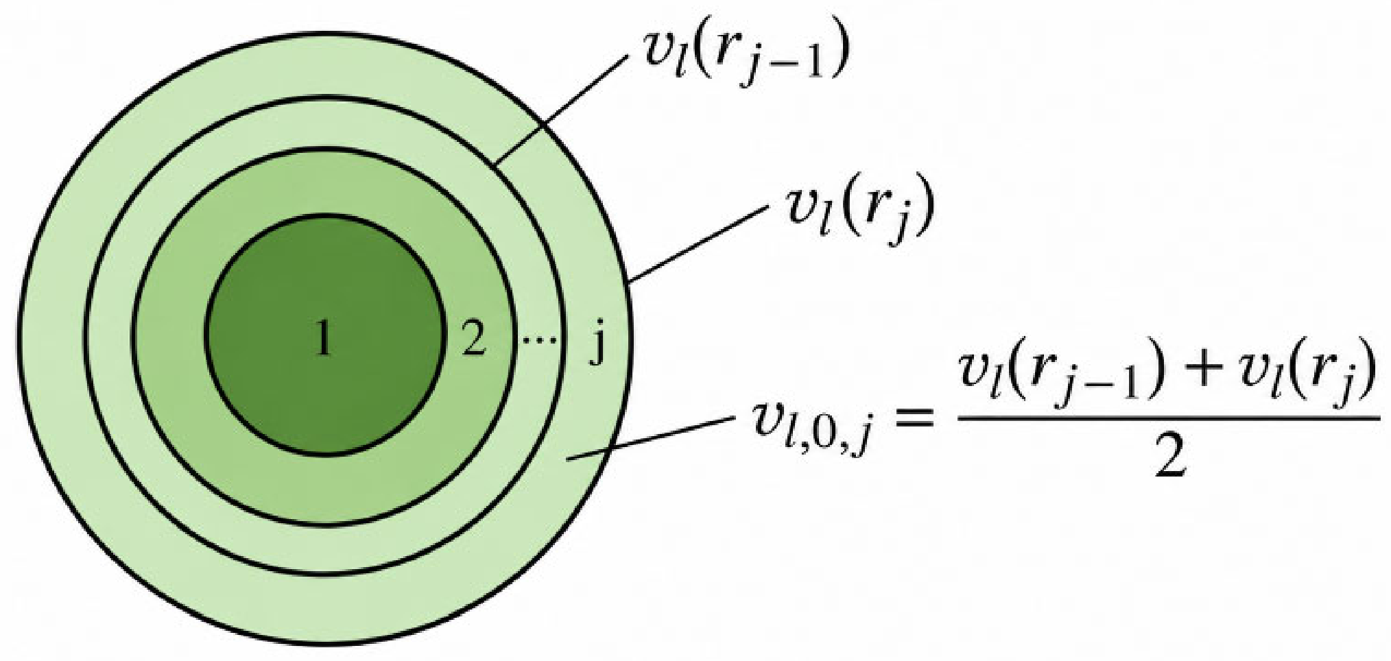
The measured and predicted particle-velocity profiles are compared in Figure 11. The model reproduced the radial trend (r = 0.949); at dp = 5.75 mm, the MAPE, RMSE, and mean bias were 17.95%, 0.288 m s−1, and +0.274 m s−1, respectively. Across the reported particle-size range, the MAPE varied from 16.60% to 19.38%.
Figure 11.
Predicted and measured particle axial-velocity profiles.
The validation results are summarized in Table 3.
Table 3.
Component-level comparison with the published vertical slurry-pipe experiment.
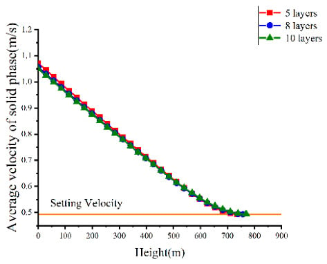
Gas-free simulations of the bottom-hole liquid–solid reverse-circulation section were used to assess the sensitivity of the predicted migration height to the tested radial resolutions (Figure 12). For Nr = 5, 8, and 10, the reported critical migration heights were 735.09, 756.88, and 770.15 m, respectively. The relative changes from five to eight layers and from eight to 10 layers were 2.96% and 1.75%, respectively. These results indicate reduced sensitivity with radial refinement but do not establish formal grid independence. The Nr = 10 case is therefore reported as the finest tested radial resolution, rather than as a verified high-accuracy solution.
Figure 12.
Effect of radial resolution on the average solid-phase velocity under gas-free conditions. The horizontal line indicates the settling-velocity threshold. Each curve terminates at the predicted critical migration height for the corresponding radial resolution.
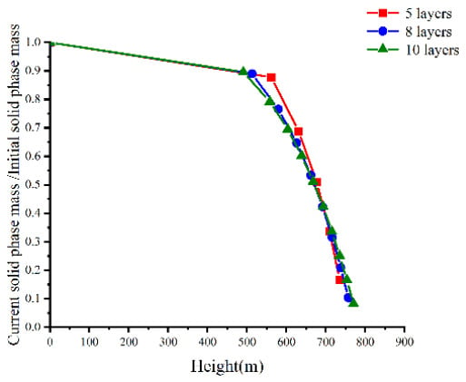
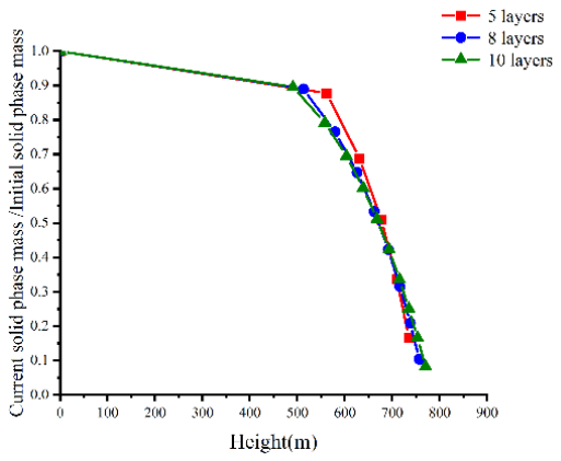
Figure 13 shows the variation in transported cuttings mass with axial height. For the five-, eight-, and 10-layer grids, the predicted cuttings-retention ratios at the critical migration height are 87.74%, 89.00%, and 89.54%, respectively. Accordingly, the fractions of the inlet cuttings mass reaching the critical migration height are 12.26%, 11.00%, and 10.46%, respectively. Within the uncoupled-layer model, these results indicate strong predicted cuttings retention below the gas-injection interface under gas-free conditions. Because radial redistribution and re-entrainment are not represented, the reported retention fractions may be overestimated and should not be interpreted as field-validated permanent-retention fractions.
Figure 13.
Transported cuttings mass for the tested radial resolutions under gas-free conditions.
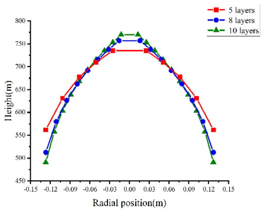
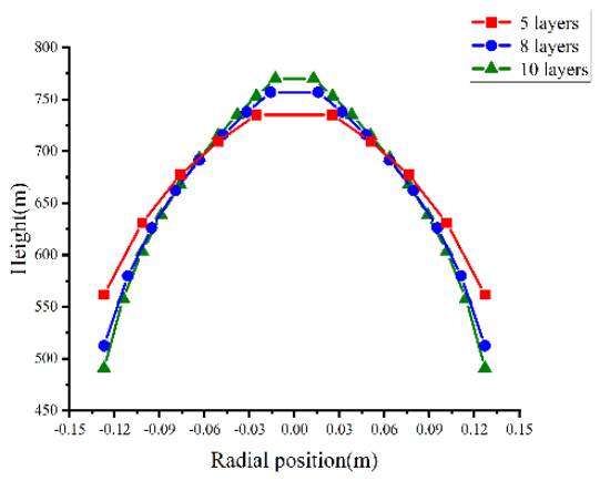
The corresponding radial distributions of the critical migration height are presented in Figure 14.
Figure 14.
Radial distribution of cuttings stopping positions (Nr = 10).
Figure 14 shows that, in the 10-layer calculation, the near-wall radial layer reaches the stopping condition first. The reported stopping position is z = 490.69 m, where vs = 0, equivalently vl = wh. Relative to the coarser tested radial resolutions, the 10-layer grid represents a narrower near-wall region and yields a lower representative local liquid carrying velocity in that region. This is a resolution-dependent numerical prediction; without independent radial velocity or particle-transport data, it cannot be interpreted as proof that the 10-layer result is physically more accurate.
Following the gas-free analysis, gas-injection heights of 600, 700, and 800 m above the bottom hole are compared at Qg = 0.100 m3 s−1. The comparison focuses on liquid carrying velocity and the fraction of inlet cuttings mass reaching the gas-injection interface.
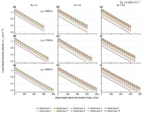
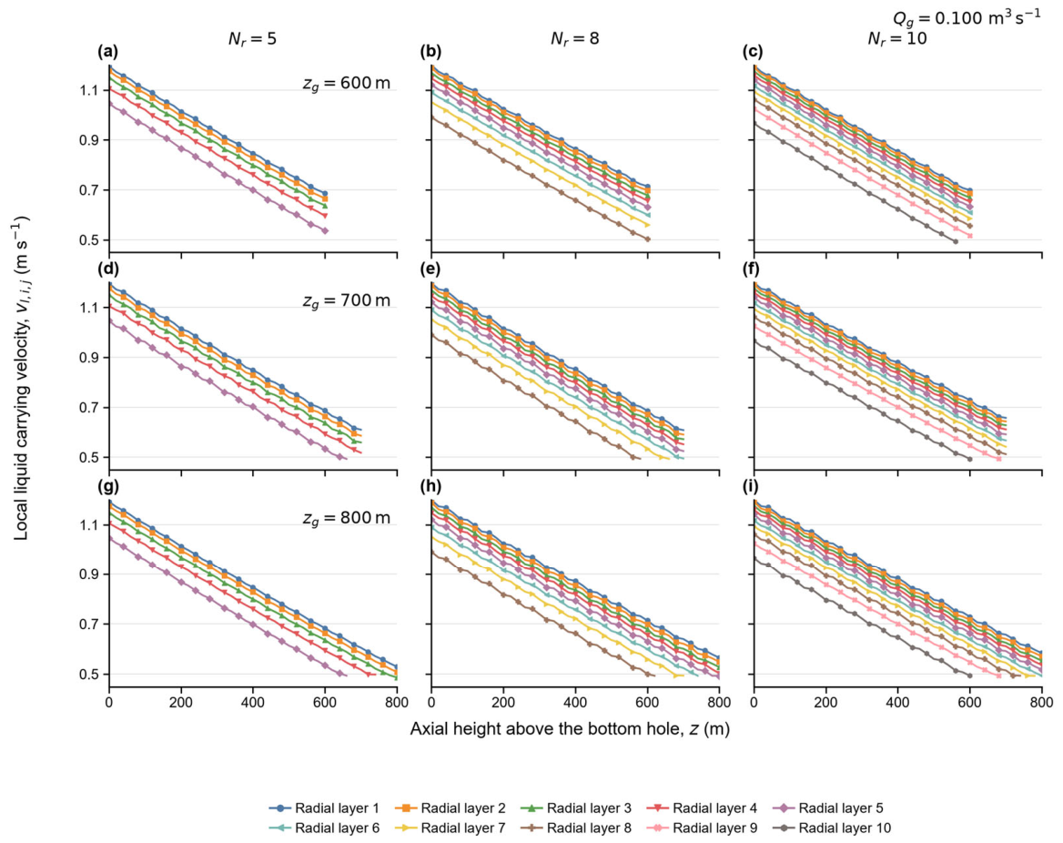
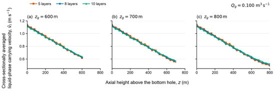
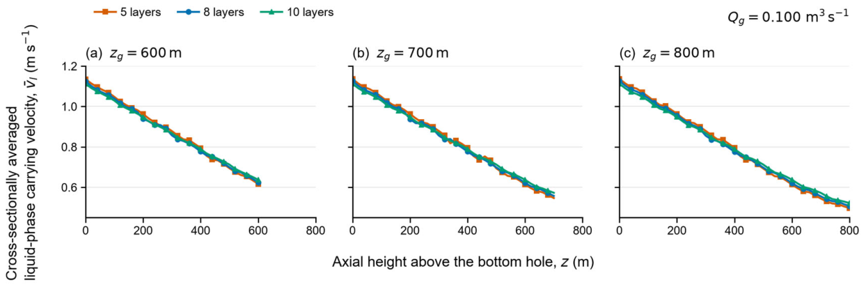
Figure 15 and Figure 16 show the axial variation in liquid-phase carrying velocity for gas-injection heights of 600, 700, and 800 m at Qg = 0.100 m3 s−1. For the 10-layer grid with injection at zg = 800 m, the predicted near-wall cuttings-migration height increases from 490.69 m under gas-free conditions to 558.19 m with gas injection. This corresponds to an additional transport distance of 67.50 m, or approximately 13.8%.
Figure 15.
Local liquid carrying velocity in each radial layer at a gas injection rate of Qg = 0.100 m3 s−1: (a) Nr = 5, Zg = 600 m; (b) Nr = 8, Zg = 600 m; (c) Nr = 10, Zg = 600 m; (d) Nr = 5, Zg = 700 m; (e) Nr = 8, Zg = 700 m; (f) Nr = 10, Zg = 700 m; (g) Nr = 5, Zg = 800 m; (h) Nr = 8, Zg = 800 m; and (i) Nr = 10, Zg = 800 m. The colored curves represent the radial layers identified in the legend.
Figure 16.
Cross-sectionally averaged liquid carrying velocity at zg = 600, 700, and 800 m above the bottom hole.
An extension of this magnitude may be relevant when assessing injection positions near a cuttings-transport limit. However, in the present case, the near-wall cuttings still stop 241.81 m below the gas-injection interface. The improvement therefore represents an extension of near-wall transport, rather than successful transfer of all near-wall cuttings into the upper gas-lift region. Its practical value must be assessed together with the transported cuttings-mass fraction, allowable bottom-hole pressure, and prediction uncertainty. The simulations alone do not establish a field-validated operational benefit.
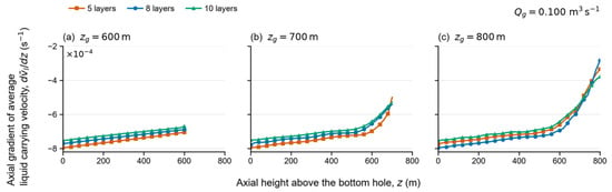
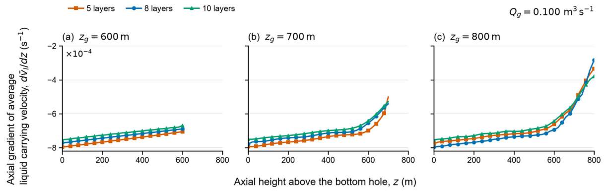
Figure 17 shows the axial gradient of the cross-sectionally averaged liquid carrying velocity, . A negative gradient indicates that this velocity decreases with axial height, whereas a less negative value indicates weaker axial attenuation. These gradients describe spatial changes in the liquid velocity, not the temporal acceleration of individual cuttings. Whether cuttings continue to migrate must instead be determined from the local net velocity, vs,i,j = vl,i,j − wh,i,j.
Figure 17.
Axial gradient of the averaged liquid carrying velocity at zg = 600, 700, and 800 m above the bottom hole.
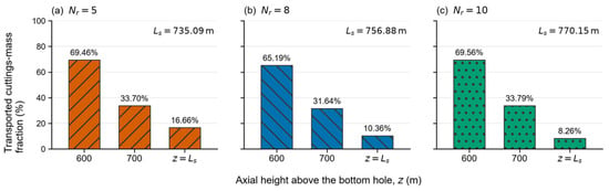
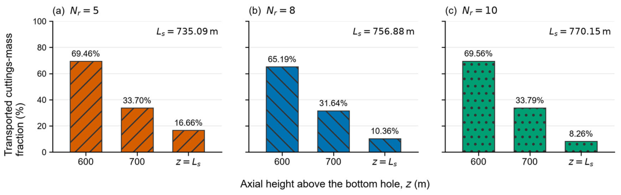
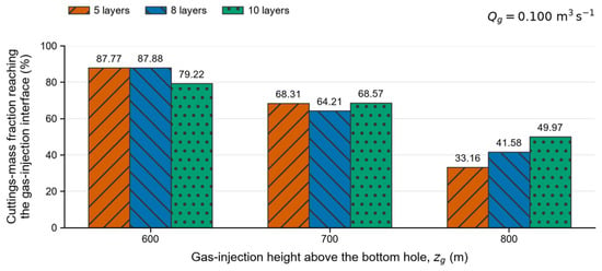
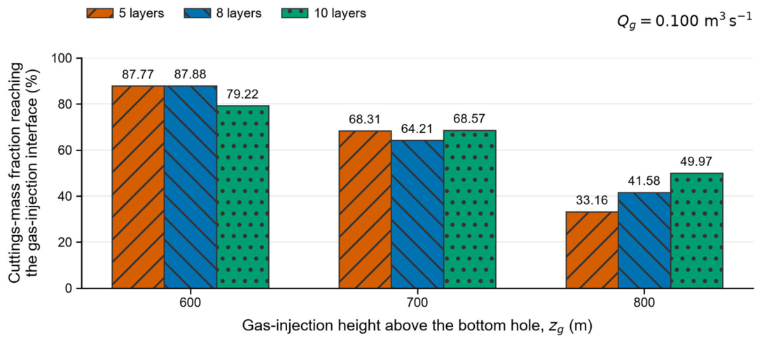
Figure 18 and Figure 19 compare the normalized transported cuttings mass under gas-free and gas-injection conditions, respectively. At gas-injection heights of 600, 700, and 800 m above the bottom hole, the fractions of the inlet cuttings mass reaching the gas-injection interface are 79.2–87.8%, 64.2–68.57%, and 33.2–49.9%, respectively. Relative to the gas-free results shown in Figure 17, gas injection increases the transported cuttings-mass fraction at the same axial height by approximately 20–30%. These values represent the fraction of inlet cuttings mass reaching the gas-injection interface, not the fraction recovered at the wellhead.
Figure 18.
Transported cuttings-mass fraction under gas-free conditions at z = 600 m, 700 m, and z = Ls.
Figure 19.
Inlet cuttings-mass fraction reaching the gas-injection interface at zg = 600, 700, and 800 m above the bottom hole.
At the finest tested reference resolution, the 600 m case produced the largest fraction of inlet cuttings mass reaching the gas-injection interface among the three discrete heights of 600, 700, and 800 m. This result provides a ranking of the tested cases for the adopted transported-mass criterion, but it does not determine a continuous optimum or a gas-injection position with meter-scale accuracy. The 13.27 m difference between the Nr = 8 and Nr = 10 migration-height predictions remains an unresolved numerical-resolution sensitivity and must be considered when interpreting the engineering significance of the comparison.
The near-wall layer reaches the stopping condition first because its liquid carrying velocity is lower than that of the central layers. Gas injection affects the lower liquid–solid region through pressure coupling at the interface, whereas a higher injection point increases the distance cuttings must travel before reaching it. Unlike the lifting-force and pressure-loss analysis of Ye et al. [32], the present model predicts layer-dependent cuttings stopping positions below the gas-injection interface. This distinction does not establish greater predictive accuracy than CFD–DEM.
These predictions are limited to the tested conditions and a dilute, stationary, vertical-pipe model. Local near-wall accumulation may weaken the dilute-phase assumption, while particle collisions, drill-pipe rotation, transient flow, and non-Newtonian fluid behavior are not resolved. The local-equilibrium algebraic-slip closure also neglects finite particle relaxation and inertial lag. Consequently, the model is not intended to resolve the entrance-acceleration region, gas-injection start-up, pulsating operation, or other rapidly varying conditions. The field-derived parameters are model inputs. The independent comparison supports the physical reasonableness of the particle-velocity closure under the tested conditions.
A structural limitation of the present reduced-order model is the absence of direct cuttings exchange between adjacent radial layers. Turbulent particle dispersion, collision-induced radial migration, and re-entrainment from the near-wall region are therefore not resolved. This simplification may bias the predictions toward persistent near-wall retention, although the magnitude of this bias cannot be quantified using the present formulation. Accordingly, the predicted stopping heights and transported-mass fractions should be interpreted as model-dependent indicators for comparing the tested operating cases rather than as absolute predictions of field-scale cuttings retention or recovery.
4. Conclusions
This study develops a radial-layered liquid–solid model that supplements existing system-level ALRC design criteria by predicting layer-dependent cuttings migration and stopping positions below the gas-injection interface at a prescribed gas flow rate. The main findings are summarized below.
Under gas-free liquid–solid reverse circulation, the near-wall radial layer reaches the stopping condition first because it has the lowest local liquid-phase carrying velocity. At the reported stopping position, vl = wh, which is equivalent to vs = 0. Across the tested radial resolutions, the uncoupled-layer model predicts that approximately 8–16% of the inlet cuttings mass reaches the reported critical migration height under gas-free conditions. Because radial redistribution and re-entrainment are not represented, these values may underestimate the actual transport capacity and should not be interpreted as field-scale permanent-retention or wellhead-recovery fractions. The greatest predicted cuttings retention occurs in the near-wall region.
For the Nr = 10 calculation, gas injection at 800 m above the bottom hole increases the predicted near-wall cuttings-migration height by 67.50 m, or approximately 13.8%, relative to the gas-free case. This increase is specific to the tested gas flow rate and reference-case parameters. However, the near-wall cuttings still stop below the injection interface, indicating improved but incomplete transport.
The velocity-gradient turning point appears when the near-wall cuttings reach the stopping condition, after which little additional cuttings mass enters the near-wall layer. Within the present continuum model, this behavior is attributed to the low near-wall liquid carrying velocity and the empirical solid–wall interaction term; individual particle–wall collisions are not resolved explicitly.
For the composite reference case at Qg = 0.100 m3 s−1, the Nr = 10 reference calculation shows that a gas-injection height of 600 m above the bottom hole gives the largest transported cuttings-mass fraction among the three tested heights of 600, 700, and 800 m. Under the prescribed operating conditions and transported-mass criterion, 600 m is therefore identified as the preferred candidate among the tested heights. It is also conditional on the no-interlayer-exchange assumption and should therefore be interpreted as the best-performing tested case within the present model, rather than as a field-validated optimum.
The proposed model provides a framework for assessing gas-injection height under prescribed operating conditions. The present calculations do not establish a general ALRC operating optimum. Broader gas-flow-rate and injection-height comparisons, together with field validation, are needed before general design recommendations can be made.
Author Contributions
P.L.: Conceptualization; Resources; Data curation; Software; Formal analysis; Validation; Methodology; Funding acquisition. J.X.: Conceptualization; Data curation; Software; Validation; Visualization; Writing—original draft; Writing—review & editing; Methodology; Project administration. C.G.: Software; Formal analysis; Validation; Project administration. Y.L.: Resources; Investigation; Visualization; Methodology; Project administration. R.Z.: Methodology; Writing—original draft; Writing—review & editing. All authors have read and agreed to the published version of the manuscript.
Funding
Sichuan Provincial Department of Education (2024NSFSC2023).
Data Availability Statement
The model input data are provided in Table 2, and the calculation workflow is shown in Figure 8 and Figure 9. The experimental benchmark conditions were obtained from Zhao et al., and nineteen measured particle velocities were digitized from Figure 11 of that publication. The digitized comparison points and derived error metrics are available from the corresponding author upon reasonable request.
Acknowledgments
This work was supported by the General Project of the Sichuan Provincial Science and Technology Education Joint Fund (Research on the Multiphase Fluid Dynamics Characteristics and Pressure Dynamic Response Mechanism of Wellbore in Gas Intrusion Compression Well Process, Grant No. 2024NSFSC2023).
Conflicts of Interest
Author Yingjie Li was employed by the company Xinjiang Oilfield Gas Production Plant. The remaining authors declare that the research was conducted in the absence of any commercial or financial relationships that could be construed as a potential conflict of interest.
Nomenclature
| Parameter definitions | ||
| Symbol | Definition | SI unit |
| A | Internal cross-sectional area of the drill pipe | m2 |
| Aj | Cross-sectional area of radial layer j | m2 |
| CD | Particle drag coefficient | – |
| Ck | Volume fraction of phase k, where k = l, s | – |
| Ck,i,j | Local volume fraction of phase k in axial cell i and radial layer j | – |
| Cl,i,j | Local liquid volume fraction in axial cell i and radial layer j | – |
| Cs,i,j | Local cuttings volume fraction in axial cell i and radial layer j | – |
| Cs,0,j | Inlet cuttings volume fraction in radial layer j | – |
| Cl,0,j | Inlet liquid volume fraction in radial layer j | – |
| Cs,A,0 | Cross-sectionally averaged inlet cuttings volume fraction | – |
| D | Internal diameter of the drill pipe | m |
| Dbit | Drill-bit or borehole diameter | m |
| dp | Equivalent diameter of a cuttings particle | m |
| Dk/Dt | Material derivative following phase k | s−1 |
| fD | Darcy friction factor for the liquid–solid flow region | – |
| fwl | Wall-interaction force density acting on the liquid phase | N m−3 |
| fws | Wall-interaction force density acting on the cuttings phase | N m−3 |
| Flift | Effective lifting force acting on the considered gas–liquid control volume | N |
| g | Gravitational acceleration | m s−2 |
| H0,j | Inlet cuttings-retention ratio in radial layer j | – |
| i | Axial-cell index | – |
| istop,j | Index of the last axial cell completed by the cuttings in radial layer j | – |
| j | Radial-layer index | – |
| k | Phase identifier, k = l, s | – |
| kv | Exponent in the turbulent radial-velocity-profile correlation | – |
| Lb | Axial length of the bottom-hole liquid–solid flow region | m |
| Ls,j | Maximum cuttings-migration height in radial layer j | m |
| Mg | Molar mass of the injected gas | kg mol−1 |
| Ms | Total interphase momentum-transfer force density acting on the cuttings phase | N m−3 |
| MD | Drag-force density acting on the cuttings phase | N m−3 |
| MVM | Virtual-mass-force density acting on the cuttings phase | N m−3 |
| MH | History-force density acting on the cuttings phase | N m−3 |
| ms,0,j | Cuttings mass assigned to the inlet material parcel in radial layer j | kg |
| mṡ | Total cuttings mass flow rate at the bottom-hole inlet | kg s−1 |
| np,0,j | Number of cuttings particles in the inlet material parcel of radial layer j | – |
| nRZ | Richardson–Zaki hindered-settling exponent | – |
| Nz | Total number of axial cells | – |
| Nr | Total number of radial layers | – |
| p | Local pressure | Pa |
| patm | Atmospheric pressure at the wellhead | Pa |
| pb | Prescribed pressure at the bottom-hole inlet, z = 0 | Pa |
| pbottom(z) | Pressure field in the bottom-hole liquid–solid region | Pa |
| plift(z) | Pressure field in the upper gas-lift region | Pa |
| Pw | Wetted perimeter of the drill pipe | m |
| Ql | Drilling-fluid volumetric flow rate | m3 s−1 |
| Ql,in | Prescribed drilling-fluid volumetric flow rate at the inlet | m3 s−1 |
| Qs | Volumetric generation rate of cuttings | m3 s−1 |
| r | Radial coordinate measured from the drill-pipe centerline | m |
| rj | Radial coordinate of the outer boundary of radial layer j | m |
| Rp | Internal radius of the drill pipe | m |
| Ru | Universal gas constant | J mol−1 K−1 |
| Rep | Particle Reynolds number | – |
| sgn(vs) | Sign function determining the direction of the wall-interaction force | – |
| t | Time variable appearing only in the general parent balance equations; it is not advanced in the reduced-order calculation | s |
| tp | Accumulated Lagrangian travel time of the cuttings | s |
| tp,i,j | Accumulated cuttings travel time at axial cell i and radial layer j | s |
| tp,stop,j | Cuttings travel time at the stopping location in radial layer j | s |
| Δtin | Material-injection interval used to define an inlet cuttings parcel | s |
| T | Local absolute temperature of the multiphase fluid | K |
| ur | Liquid–solid relative velocity | m s−1 |
| Vp | Volume of an individual cuttings particle | m3 |
| vl | Absolute axial liquid-phase carrying velocity in the pipe-fixed frame | m s−1 |
| vs | Net absolute axial cuttings velocity in the pipe-fixed frame | m s−1 |
| vl,i,j | Local liquid-phase carrying velocity in axial cell i and radial layer j | m s−1 |
| vs,i,j | Local net absolute cuttings velocity in axial cell i and radial layer j | m s−1 |
| vl,0,j | Inlet liquid-phase carrying velocity in radial layer j | m s−1 |
| vs,0,j | Inlet net absolute cuttings velocity in radial layer j | m s−1 |
| vl,max | Maximum liquid-phase carrying velocity at the drill-pipe centerline | m s−1 |
| vls | Cross-sectionally averaged velocity of the liquid–solid mixture | m s−1 |
| vm | Cross-sectionally averaged velocity of the gas–liquid–solid mixture | m s−1 |
| vROP | Rate of penetration | m s−1 |
| wt0 | Terminal settling velocity of an isolated particle relative to the liquid | m s−1 |
| wt0,i,j | Local single-particle terminal settling velocity in axial cell i and radial layer j | m s−1 |
| wh | Hindered-settling velocity of the cuttings relative to the liquid, defined as positive downward | m s−1 |
| wh,i,j | Local hindered-settling velocity in axial cell i and radial layer j | m s−1 |
| z | Axial coordinate measured upward from the bottom hole | m |
| zi | Axial coordinate of cell boundary i | m |
| zg | Axial position of the gas-injection interface measured from the bottom hole | m |
| zs,j(tp) | Axial position of the cuttings in radial layer j at the corresponding travel time | m |
| Δzi | Axial length of cell i | m |
| εg | Gas volume fraction in the gas-lift region | – |
| εl | Liquid volume fraction in the gas-lift region | – |
| λgls | Darcy friction factor for the gas–liquid–solid mixture | – |
| μl | Dynamic viscosity of the liquid phase | Pa s |
| μls | Effective dynamic viscosity of the liquid–solid mixture | Pa s |
| ρl | Liquid density | kg m−3 |
| ρs | Cuttings density | kg m−3 |
| ρg | Density of the injected gas | kg m−3 |
| ρls | Density of the liquid–solid mixture | kg m−3 |
| ρgl | Density of the gas–liquid mixture | kg m−3 |
| ρgls | Density of the gas–liquid–solid mixture | kg m−3 |
| τw,s | Magnitude of the cuttings–wall shear stress | Pa |
| Ω | Volume of the gas–liquid mixture in the considered control volume | m3 |
| Qg | Gas-injection volumetric flow rate | m3 s−1 |
| Subscripts | ||
| Subscript | Definition | |
| 0 | Bottom-hole inlet | |
| A | Cross-sectionally averaged quantity | |
| atm | Atmospheric condition | |
| bottom | Bottom-hole liquid–solid region | |
| g | Gas phase | |
| gl | Gas–liquid mixture | |
| gls | Gas–liquid–solid mixture | |
| i | Axial cell | |
| in | Inlet condition | |
| j | Radial layer | |
| l | Liquid phase | |
| ls | Liquid–solid mixture | |
| lift | Upper gas-lift region | |
| max | Maximum value | |
| p | Particle | |
| s | Solid or cuttings phase | |
| stop | Cuttings stopping location | |
| w | Drill-pipe wall | |
Appendix A
Appendix A.1. Spatial and Radial Discretization
The bottom-hole liquid–solid flow region is discretized using a uniform axial grid and equal-area radial layers. The axial spacing used in the reported calculations is Δz = 1.002130926m.
For a prescribed gas-injection height zg, the number of axial cells is calculated as Nz = ceil(zg/Δz).
The radial layers are defined by equal cross-sectional areas:
The calculations use Nr = 5, 8, and 10. The calculation advances from one axial cell to the next. The variable tp denotes the accumulated Lagrangian travel time of the cuttings. It is not an Eulerian time variable, and no independent Eulerian time step is used.
Appendix A.2. Radial-Layered Spatial-Marching Algorithm
Input: D, Dbit, Ql, Qg, zg, ρl, ρs, μl, dp, Nr, Nz, Δz.
- Set the pipe radius as Rp = D/2.
- Define the equal-area radial layers using
- 3.
- For each radial layer, set the accumulated cuttings travel time tp = 0, and initialize the inlet cuttings mass ms,0,j.
- 4.
- For each axial cell i = 1,…,Nz, calculate the local pressure gradient and liquid carrying velocity vl,i,j.
- 5.
- Calculate the isolated-particle terminal settling velocity wt0,i,j.
- 6.
- Apply the Richardson–Zaki relation to obtain the hindered-settling velocity wh,i,j.
- 7.
- Calculate the net cuttings velocity vs,i,j.
- 8.
- If vs,i,j ≤ 0, record the current position as the model-predicted stopping height Ls,j and terminate axial marching for radial layer j. Under the uncoupled-layer approximation, no subsequent radial redistribution or re-entrainment is calculated.
- 9.
- If vs,i,j > 0, update the accumulated travel time and transported cuttings mass, and advance to the next axial cell.
- 10.
- If the cuttings reach the gas-injection interface, z ≥ zg, record the cuttings mass reaching the interface.
- 11.
- Repeat Steps 3–7 for all radial layers.
- 12.
- Integrate the layer-dependent results to obtain the transported cuttings-mass fraction and the stopping positions of the radial layers.
The term “iteration” in this procedure refers to spatial marching through successive axial cells. The reported calculation does not introduce an independent Eulerian time-step convergence parameter.
Appendix A.3. Input and Closure Information
The physical properties and operating conditions are provided in Table 2. The closure relations include the Darcy–Weisbach pressure-loss formulation, the Colebrook friction-factor correlation, the radial liquid-velocity profile, the particle-drag relation, the Richardson–Zaki hindered-settling relation, the mixture-viscosity relation, and the wall-interaction-force relation described in Section 2.2 and Section 2.3.
References
- Zang, Y.; Chen, Z.; Wang, Y.; Zhang, Y.; Xu, S.; Xie, J.; Chen, W. Study on the Lost Circulation Mechanism of Polymer-Based Drilling Fluid Systems in Deep Fractured Shale. Polymers 2025, 17, 2929. [Google Scholar] [CrossRef] [Scilit] [PubMed]
- Yang, J.; Sun, J.; Bai, Y.; Lv, K.; Zhang, G.; Li, Y. Status and prospect of drilling fluid loss and lost circulation control technology in fractured formation. Gels 2022, 8, 260. [Google Scholar] [CrossRef] [Scilit] [PubMed]
- Albattat, R.; Hoteit, H. Modeling Lost-Circulation into Fractured Formation in Rock Drilling Operations; IntechOpen: London, UK, 2021. [Google Scholar]
- Su, X.M.; Wang, X.D.; Yuan, Y.; Yun, R.; Wang, G. Cavitation-Induced Shear Failure Mechanism of Fractured Plugging Zone and Structure Strengthening Method for Lost Circulation Control in High-Temperature and High-Pressure Fractured Gas Reservoirs. Geofluids 2024, 2024, 8856179. [Google Scholar] [CrossRef] [Scilit]
- Zheng, B.; Zheng, X.; Duan, C.; Ye, H. Discussion on stability and applicability of gas lift reverse circulation drilling. Explor. Eng. (Rock Soil Drill. Tunneling) 2020, 47, 13–18. [Google Scholar]
- Guo, L.H.; Cheng, H.; Yao, Z.S.; Rong, C.; Lin, J.; Wang, X. Mathematical model of velocity and distribution law in gas lift reverse circulation well washing flow field for drilling shaft sinking. Sci. Rep. 2024, 14, 27327. [Google Scholar] [CrossRef] [Scilit] [PubMed]
- Zhao, C.; Wang, Y.; Nie, D.; Wang, L. Gas lift reverse circulation drilling technology for D19 well in broken thermal reservoir in Xiong’an New Area. Drill. Eng. 2022, 49, 137–143. [Google Scholar]
- Wu, X.; Feng, Y.; Du, Y.; Gao, P.; Zhao, Y.; Wang, X.; Tang, X.; Wang, Q. Simulation analysis of the flow field of the air lift reverse circulation dual wall drill tool. Drill. Eng. 2022, 49, 83–91. [Google Scholar]
- Zhang, Y.; Zhang, J. Technical improvements and application of air-lift reverse circulation drilling technology to ultra-deep geothermal well. Procedia Eng. 2014, 73, 243–251. [Google Scholar] [CrossRef] [Scilit]
- Enany, P.; Shevchenko, O.; Drebenstedt, C. Experimental evaluation of airlift performance for vertical pumping of water in underground mines. Mine Water Environ. 2021, 40, 970–979. [Google Scholar] [CrossRef] [Scilit] [PubMed]
- Chen, Y.; Li, W.; Wang, X.; Wu, P.; Wan, X.; Wang, Z.; Li, J.; Sun, X. A Numerical Simulation of the Effect of Drilling Fluid Rheology on Cutting Migration in Horizontal Wells at Different Drilling Fluid Temperatures. Processes 2024, 12, 2428. [Google Scholar] [CrossRef] [Scilit]
- Wei, L.; Honra, J. Impact of Rock Cuttings on Downhole Fluid Movement in Polycrystalline Diamond Compact (PDC) Bits, Computational Fluid Dynamics, Simulation, and Optimization of Hydraulic Structures. Fluids 2025, 10, 13. [Google Scholar] [CrossRef] [Scilit]
- Li, Z.; Zhang, B.; Jiang, L.; Yang, T.; Luo, T.; Cao, X.; Yang, X.; Li, G.; Li, H.; Sun, X.; et al. Cuttings-Bed Dynamics and Wellbore Cleaning: A Critical Review of Multiscale Modeling, Multiphase Flow, and Cross-Scale Validation. Processes 2026, 14, 2245. [Google Scholar] [CrossRef] [Scilit]
- Zakeri, A.; Alizadeh Behjani, M.; Hassanpour, A. Fully Coupled CFD-DEM Simulation of Oil Well Hole Cleaning: Effect of Mud Hydrodynamics on Cuttings Transport. Processes 2024, 12, 784. [Google Scholar] [CrossRef] [Scilit]
- Akhshik, S.; Behzad, M.; Rajabi, M. CFD-DEM approach to investigate the effect of drill pipe rotation on cuttings transport behavior. J. Pet. Sci. Eng. 2015, 127, 229–244. [Google Scholar] [CrossRef] [Scilit]
- Liu, Y.; Gao, D.; Li, X.; Qin, X.; Li, H.; Liu, H. Investigating the jet comminuting process in cuttings transport by coupling the CFD/DEM method and bonded-particle model. SPE J. 2019, 24, 2020–2032. [Google Scholar] [CrossRef] [Scilit]
- Deng, S.; He, J.; Kang, B.; Liu, W.; Ling, D.; Pei, C. Wellbore Flow Model and Process Optimization for Gas-Lift Leakage Drilling for Shallow Shale Formations. ACS Omega 2022, 7, 7806–7815. [Google Scholar] [CrossRef] [Scilit] [PubMed]
- Li, Q.; Zhang, X.; Li, Z.; Li, J.; Dai, F. Annular Aerated Gas-lift Reverse Circulation Drilling Technology and Key Parameters Design. J. Southwest Pet. Univ. (Sci. Technol. Ed.) 2021, 43, 35–43. [Google Scholar]
- Zeng, C.; Chen, Y.; Yan, X. Transportation of cuttings through drill rods during reverse-circulation reaming. Tunn. Undergr. Space Technol. 2022, 126, 104544. [Google Scholar] [CrossRef] [Scilit]
- Sun, S.; Bo, K.; Jia, R.; Cao, P.; Chen, B.; Guo, M. Experimental investigation and CFD simulation of multiphase flow behavior in air reverse circulation drilling. Adv. Powder Technol. 2023, 34, 104168. [Google Scholar] [CrossRef] [Scilit]
- Guo, L.H.; Cheng, H.; Yao, Z.S.; Rong, C.; Wang, Z.; Wang, X. CFD-DEM method is used to study the multi-phase coupling slag discharge flow field of gas-lift reverse circulation in drilling shaft sinking. Sci. Rep. 2024, 14, 13853. [Google Scholar] [CrossRef] [Scilit] [PubMed]
- Zhang, F.; Miska, S.; Yu, M.; Ozbayoglu, E. A unified transient solid-liquid two-phase flow model for cuttings transport: Modelling part. J. Pet. Sci. Eng. 2018, 166, 146–156. [Google Scholar] [CrossRef] [Scilit]
- Hashemi, S.; Sadighian, A.; Shah, S.; Sanders, R. Solid velocity and concentration fluctuations in highly concentrated liquid-solid (slurry) pipe flows. Int. J. Multiph. Flow 2014, 66, 46–61. [Google Scholar] [CrossRef] [Scilit]
- Kharlamov, S.N.; Janghorbani, M.; Bryskin, M.R. Aspects of computer simulation of transport and cleaning processes from cuttings in horizontal well sections. Math. Models Comput. Simul. 2023, 15, 502–519. [Google Scholar] [CrossRef] [Scilit]
- Xu, Z.; Song, X.; Zhu, Z. Development of elastic drag coefficient model and explicit terminal settling velocity equation for particles in viscoelastic fluids. SPE J. 2020, 25, 2962–2983. [Google Scholar] [CrossRef] [Scilit]
- Hou, Z.; Yuan, Y.; Chen, Y.; Jiang, E.; Wang, H.; Zhang, X. A Review of the Settling Law of Drill Cuttings in Drilling Fluids. Processes 2023, 11, 3165. [Google Scholar] [CrossRef] [Scilit]
- Zhu, J.; Du, Y.; Li, M.; Fu, M.; Han, X.; Peng, F.; Ruan, R.; Shen, Y. Evaluate the performance of the vertically upward gas-liquid two-phase flow in an airlift pump system. Int. J. Multiph. Flow 2024, 181, 105016. [Google Scholar] [CrossRef] [Scilit]
- Hanafizadeh, P.; Ghanbarzadeh, S.; Saidi, M.H. Visual technique for detection of gas-liquid two-phase flow regime in the airlift pump. J. Pet. Sci. Eng. 2011, 75, 327–335. [Google Scholar] [CrossRef] [Scilit]
- Fujimoto, H.; Nagatani, T.; Takuda, H. Performance characteristics of a gas-liquid-solid airlift pump. Int. J. Multiph. Flow 2005, 31, 1116–1133. [Google Scholar] [CrossRef] [Scilit]
- Catrawedarma, I.G.N.B.; Deendarlianto; Indarto. Statistical characterization of flow structure of air-water two-phase flow in airlift pump-bubble generator system. Int. J. Multiph. Flow 2021, 138, 103596. [Google Scholar] [CrossRef] [Scilit]
- Zhao, L.; Wang, T.; Han, W. Study on velocity distribution of large particle in vertical slurry pipeline. Meas. Control 2019, 52, 1282–1288. [Google Scholar] [CrossRef] [Scilit]
- Ye, H.; Lai, Z.; Tian, L.; Zhang, R.; Liu, B.; Zheng, X. Air-Lifting Reverse-Circulation Drilling in Deep Geothermal Wells and the Effect of Dual-Wall Drill Pipe Depth Down the Hole. Energies 2025, 18, 1224. [Google Scholar] [CrossRef] [Scilit]

Disclaimer/Publisher’s Note: The statements, opinions and data contained in all publications are solely those of the individual author(s) and contributor(s) and not of MDPI and/or the editor(s). MDPI and/or the editor(s) disclaim responsibility for any injury to people or property resulting from any ideas, methods, instructions or products referred to in the content. |
© 2026 by the authors. Licensee MDPI, Basel, Switzerland. This article is an open access article distributed under the terms and conditions of the Creative Commons Attribution (CC BY) license.