A Sub-Hertz-Resolution RF/DC Driver Platform for Quadrupole Mass Filtering Processes: Coupled Modeling, Hardware Design, and Benchtop Characterization

Abstract

In quadrupole mass filtering processes, ion trajectory stability is governed by the Mathieu parameters ($a,q$), which scale inversely with the square of the excitation frequency (${\omega }^{-2}$). High-quality-factor ($Q\ge 100$) series resonant networks are widely employed for passive radio-frequency (RF) voltage step-up. However, their narrow passbands render the output amplitude vulnerable to temperature-induced capacitive detuning. Furthermore, conventional microcontroller-based Direct Digital Synthesis (DDS) architectures rely on integer register parsing, constraining the tuning resolution to ≥1 Hz and introducing quantization errors during frequency scanning and tracking. This paper presents the coupled modeling, hardware design, and benchtop characterization of a software-defined RF/DC driver platform with 0.1 Hz frequency resolution for resonant quadrupole mass filters. Numerical modeling coupling fourth-order Runge–Kutta (RK4) ion dynamics with RLC transfer functions demonstrates that a 0.1 Hz frequency increment restricts stability parameter shifts to $\Delta q/q<2\times {10}^{-7}$, limits detuning voltage attenuation to $\Delta V/V_0<{10}^{-5}$, and eliminates peak apex truncation at mass resolving powers $R>1200$. The hardware platform integrates an STM32 microcontroller, an AD9954 DDS core (400 MSPS), an IEEE-754 32-bit floating-point Ethernet communication pipeline, a 16-bit bipolar DC bias stage (0.1 mV step resolution), and an in-loop baseband telemetry channel. Benchtop measurements demonstrate continuous RF generation from 10 Hz to 10 MHz with a relative frequency error below 0.070%. On a 1.0 MHz series resonant network loaded with a 50 pF equivalent capacitance, thermal measurements reveal an open-loop start-up frequency scatter of 0.266% (2.66 kHz), demonstrating the necessity of sub-Hertz frequency correction to restore resonance. The telemetry channel achieves an acquisition stability relative standard deviation (RSD) of $1.2\times {10}^{-5}$ via a 500-sample moving-average filter, enabling closed-loop frequency tracking to maintain the normalized RF amplitude within $99.55\%$ to $100.00\%$ across a 60-min thermal cycle. Characterized on a benchtop equivalent load, this hardware platform provides a deterministic electronic foundation for dynamic resonance re-centering and stable ion transmission in high-Q quadrupole systems.

1. Introduction

Quadrupole mass spectrometers (QMSs) and linear multipole devices are widely used in chemical analysis and analytical instrumentation [1,2] due to their compact structure, continuous-beam operation, and moderate vacuum requirements [3,4]. A quadrupole electric field is formed by applying a radio-frequency (RF) potential $V\cos \left(\omega t\right)$ and a static direct-current (DC) voltage U with opposite polarities to diagonally paired, parallel electrode rods [5,6,7,8]. The transverse motion of ions within this field is governed by the Mathieu differential equations, where trajectory stability depends on the dimensionless parameters a and q [9,10,11,12]. Because these parameters scale inversely with the square of the excitation frequency ($a,q\propto {\omega }^{-2}$) [10,12], the mass-filtering resolution, transmission efficiency, and operational stability depend directly on the amplitude stability, phase fidelity, and frequency precision of the driving electronics.

To deliver high-voltage sinusoidal waveforms (hundreds to thousands of volts peak-to-peak) with low power dissipation, high-quality-factor ($Q\ge 100$) series resonant networks—such as air-core RLC tanks or helical resonators—are commonly employed as passive step-up stages [13,14,15]. However, operating at high-quality factors narrows the operational passband ($\Delta f_{3\mathrm{dB}}=f_0/Q$), making the output voltage sensitive to load impedance variations [14]. In practical assemblies, ambient temperature changes induce sub-picofarad drifts in the inter-electrode parasitic capacitance ($\Delta C$), which shift the loaded resonant frequency of the network [14,15]. Traditional mechanical compensation methods, such as adjustable inductor taps or motorized variable capacitors [16], are constrained by mechanical backlash, contact wear, and slow response times, limiting dynamic correction during operation.

Direct Digital Synthesis (DDS) and digital RF generators allow for electronic adjustment of the driving frequency by updating the digital Frequency Tuning Word (FTW) [17,18,19,20,21,22,23,24]. Nevertheless, existing DDS-based quadrupole drivers exhibit several practical limitations. First, dedicated embedded implementations often handle target frequencies as integer values in firmware or communication protocols, constraining the command resolution to ≥1 Hz or $1\mathrm{kHz}$ [19,20]. In high-Q resonant networks, kilohertz frequency offsets produce phase shifts and voltage attenuation exceeding $10\%$, which alters the mass scan line $a/q=2U/V$ [17,20]. In frequency-scanned modes, a 1 Hz stepping interval also introduces discrete quantization steps across narrow stability peaks. Second, typical drivers are designed as standalone units with narrow output bandwidths (<2 MHz) [18,20,24], limiting their adaptability to multi-mode operations or integration into networked laboratory platforms. Finally, existing studies typically treat the RF driver as an isolated circuit stage [15,22,24], lacking quantitative analysis that links digital frequency resolution to resonant circuit detuning and ion stability limits.

To address these limitations, this paper presents the coupled numerical modeling, hardware design, and benchtop characterization of a software-defined RF/DC driver platform with 0.1 Hz frequency resolution for resonant quadrupole loads. A coupled numerical model combining fourth-order Runge–Kutta (RK4) ion dynamics with high-Q RLC transfer functions is developed to evaluate frequency detuning and quantization effects. The simulation results show that a 0.1 Hz frequency step size restricts stability parameter shifts to $\Delta q/q<2\times {10}^{-7}$, eliminates peak apex truncation in simulated frequency-scanned regimes ($R>1200$), and bounds theoretical resonant voltage attenuation to $\Delta V/V_0<{10}^{-5}$. On the hardware level, an embedded platform integrating an STM32 microcontroller, an AD9954 DDS core (400 MSPS), and a W5500 Ethernet controller is realized. By implementing an IEEE-754 32-bit floating-point communication protocol, the system avoids integer truncation in command parsing and achieves deterministic 0.1 Hz frequency stepping across six decades from 10 Hz to 10 MHz. In addition, the driver incorporates a 16-bit bipolar DC bias generator offering 0.1 mV step resolution and an in-loop baseband telemetry channel, where a firmware-implemented 500-sample moving-average filter yields an acquisition stability relative standard deviation (RSD) of $1.2\times {10}^{-5}$. Finally, benchtop experiments on a 50 pF equivalent capacitive load are conducted to evaluate wideband frequency synthesis accuracy, open-loop thermal scatter, closed-loop resonance tracking, and DC output linearity.

2. Theoretical Principles and Simulation Modeling

2.1. Quadrupole Ion Dynamics and the Mathieu Equation

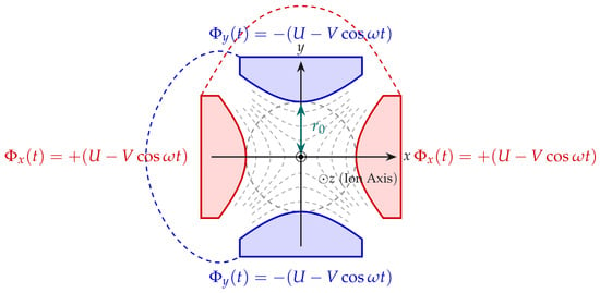
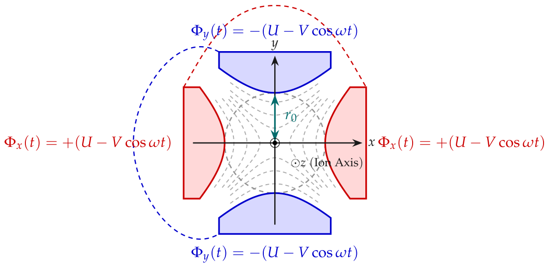
An ideal quadrupole mass filter consists of four hyperbolic electrodes aligned parallel to the longitudinal z-axis, as illustrated in Figure 1 [6,9]. The inscribed radius from the central axis to each electrode tip is denoted by $r_0$. Opposite electrodes are electrically connected, and complementary potentials are applied to the x- and y-electrode pairs:

$${\mathsf{\Phi }}_x\left(t\right)=+(U-V\cos \omega t)$$

(1)

$${\mathsf{\Phi }}_y\left(t\right)=-(U-V\cos \omega t)$$

(2)

where U is the static DC voltage, V is the zero-to-peak amplitude of the RF excitation potential, $\omega =2\pi f_0$ denotes the angular frequency, and t is time.

Figure 1. Cross-section of the hyperbolic quadrupole analyzer showing the coordinate system, inscribed field radius $r_0$, and applied RF/DC potentials.

Assuming ideal hyperbolic boundaries without axial fringing fields, the two-dimensional potential distribution $\mathsf{\Phi }(x,y,t)$ satisfies Laplace’s equation ${\nabla }^2\mathsf{\Phi }=0$ [7,8]:

$$\mathsf{\Phi }(x,y,t)=(U-V\cos \omega t){\displaystyle \frac{x^2-y^2}{r_0^2}}$$

(3)

The electric field components are obtained from $\mathbf{E}=-\nabla \mathsf{\Phi }$:

$$E_x=-{\displaystyle \frac{\partial \mathsf{\Phi }}{\partial x}}=-{\displaystyle \frac{2(U-V\cos \omega t)}{r_0^2}}x,E_y=-{\displaystyle \frac{\partial \mathsf{\Phi }}{\partial y}}=+{\displaystyle \frac{2(U-V\cos \omega t)}{r_0^2}}y$$

(4)

For an ion of mass m and net charge $ze$ (where $e=1.602\times {10}^{-19}\mathrm{C}$ is the elementary charge and z is the charge state), the equations of motion in the transverse plane are:

$$m{\displaystyle \frac{{\mathrm{d}}^{2}x}{\mathrm{d}{t}^2}}+{\displaystyle \frac{2ze}{r_0^2}}(U-V\cos \omega t)x=0$$

(5)

$$m{\displaystyle \frac{{\mathrm{d}}^{2}y}{\mathrm{d}{t}^2}}-{\displaystyle \frac{2ze}{r_0^2}}(U-V\cos \omega t)y=0$$

(6)

Introducing the dimensionless time variable $\xi =\omega t/2$ and the stability parameters $a_u$ and $q_u$ ($u=x,y$) [10,11],

$$a_x=-a_y={\displaystyle \frac{8zeU}{m{\omega }^2{r}_0^2}},q_x=-q_y={\displaystyle \frac{4zeV}{m{\omega }^2{r}_0^2}}$$

(7)

transforms Equations (5) and (6) into the Mathieu equations:

$${\displaystyle \frac{{\mathrm{d}}^{2}u}{\mathrm{d}{\xi }^2}}+(a_u-2q_u\cos 2\xi )u=0,(u=x,y)$$

(8)

According to Floquet theory, bounded ion trajectories exist within overlapping stability regions in $(a,q)$ space. For mass filtration, the operating point is positioned near the apex of the first stability zone at $(q_{\mathrm{apex}},a_{\mathrm{apex}})\approx (0.7060,0.2370)$ [6,12].

The mass scan line is defined by the constant ratio:

$${\displaystyle \frac{a}{q}}={\displaystyle \frac{2U}{V}}=\mathrm{const}$$

(9)

Assuming fixed potential amplitudes (U and V), differentiating Equation (7) with respect to the excitation frequency $f_0=\omega /\left(2\pi \right)$ gives the parametric sensitivity

$${\left.{\displaystyle \frac{\mathrm{d}a}{a}}\right|}_U={\left.{\displaystyle \frac{\mathrm{d}q}{q}}\right|}_V=-2{\displaystyle \frac{\mathrm{d}{f}_0}{f_0}}$$

(10)

Equation (10) indicates that a relative frequency deviation induces a twofold relative shift in the stability parameters. In broadband or non-resonant driving modes where voltage amplitude is independent of frequency, this relation directly determines the required frequency stepping resolution.

When driving a series resonant network, the delivered RF amplitude $V\left(f_0\right)=V_{\mathrm{in}}\left|H\left(f_0\right)\right|$ depends on frequency through the network transfer function $H\left(f_0\right)$. The total sensitivity of the stability parameter q is given by:

$${\displaystyle \frac{\mathrm{d}q}{q}}={\displaystyle \frac{\mathrm{d}V\left(f_0\right)}{V}}-2{\displaystyle \frac{\mathrm{d}{f}_0}{f_0}}={\displaystyle \frac{1}{\left|H\right(f_0\left)\right|}}{\displaystyle \frac{\partial \left|H\right(f_0\left)\right|}{\partial f_0}}\mathrm{d}{f}_0-2{\displaystyle \frac{\mathrm{d}{f}_0}{f_0}}$$

(11)

At resonance ($f_0=f_{\mathrm{res}}$), the first derivative of the transfer function magnitude vanishes ($\partial \left|H\right|/\partial f_0=0$), and Equation (11) simplifies to Equation (10). Off resonance, however, the steep roll-off of a high-Q passband causes voltage attenuation that further displaces the operating point in $(a,q)$ space. Consequently, sub-Hertz frequency granularity (0.1 Hz) provides the resolution needed for precise resonance centering ($\partial \left|H\right|/\partial f_0\approx 0$) in resonant step-up networks and smooth parameter tracking in frequency-scanned modes.

2.2. Numerical Simulation of Ion Trajectory Dynamics and Frequency Sensitivity

To evaluate the effect of RF offsets and discrete tuning quantization on ion transmission, ion trajectories were simulated by numerically integrating the equations of motion using a fourth-order Runge–Kutta (RK4) method in MATLAB (Version R2023b, The MathWorks, Inc., Natick, MA, USA) [10,12].

In the time domain, the transverse equations of motion [Equations (5) and (6)] are formulated as a first-order state-space system:

$$\left\{\begin{array}{c}{\dot{x}}_1=x_2\hfill \\ {\dot{x}}_2=-{\displaystyle \frac{2ze}{m{r}_0^2}}\left(U-V\cos \omega t\right)x_1\hfill \\ {\dot{y}}_1=y_2\hfill \\ {\dot{y}}_2=+{\displaystyle \frac{2ze}{m{r}_0^2}}\left(U-V\cos \omega t\right)y_1\hfill \end{array}\right.$$

(12)

where $x_1=x\left(t\right)$, $x_2=\dot{x}\left(t\right)$, $y_1=y\left(t\right)$, and $y_2=\dot{y}\left(t\right)$ denote the transverse positions and velocity components, respectively. Equation (12) is numerically integrated using a fixed RK4 time step of $\Delta t=1.0\mathrm{ns}$ (corresponding to $1000\mathrm{integration}\mathrm{steps}$ per $1.0\mathrm{MHz}$ RF cycle) to accurately resolve both low-frequency secular motion and high-frequency RF micromotion. Step-halving convergence tests ($\Delta t=0.5\mathrm{ns}$ versus $1.0\mathrm{ns}$) confirmed that the relative trajectory position error remains below ${10}^{-6}$ over the entire transit duration.

The simulation tracks an ensemble of $N=2000$ test ions ($z=1$, $m/z=100\mathrm{Th}$) injected along the longitudinal z-axis with an initial axial kinetic energy of $E_z=5.0\mathrm{eV}$ into a quadrupole analyzer with $r_0=4.0\mathrm{mm}$ and length $L_z=150\mathrm{mm}$. Initial entrance positions $(x_0,y_0)$ are sampled from a uniform distribution over an aperture of radius $r_{\mathrm{in}}=0.1r_0$, while initial transverse velocities follow a Maxwell–Boltzmann distribution at $T=300\mathrm{K}$. Initial RF injection phases ${\xi }_0=\omega t_0/2$ are uniformly distributed over $[0,\pi )$ to model continuous beam injection. An ion is considered transmitted if its instantaneous radial displacement remains within the inscribed electrode aperture throughout the transit time (assuming ideal hyperbolic fields without axial fringing-field losses):

$$r\left(t\right)=\sqrt{x_1{\left(t\right)}^2+y_1{\left(t\right)}^2}<r_0,\forall t\in [0,t_{\mathrm{transit}}]$$

(13)

where $t_{\mathrm{transit}}=L_z/\sqrt{2E_z/m}\approx 48.3\mathsf{\mu }\mathrm{s}$ is the nominal axial transit duration (comprising $\approx 48.3$ RF cycles). Parametric sensitivity evaluations indicate that varying the scan-line ratio $a/q=2U/V$ by $\pm 0.01\%$ near the stability apex shifts the peak transmission efficiency by ≈4.2% and alters the resolving power R by $\pm 65$, whereas the 0.1 Hz frequency quantization threshold and the 50% detuning passband ($|\Delta f|\le 150\mathrm{Hz}$) remain invariant across initial axial ion energies $E_z\in [3.0,7.0]\mathrm{eV}$.

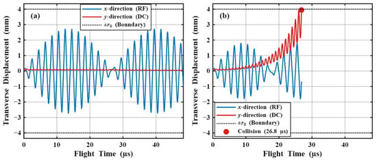
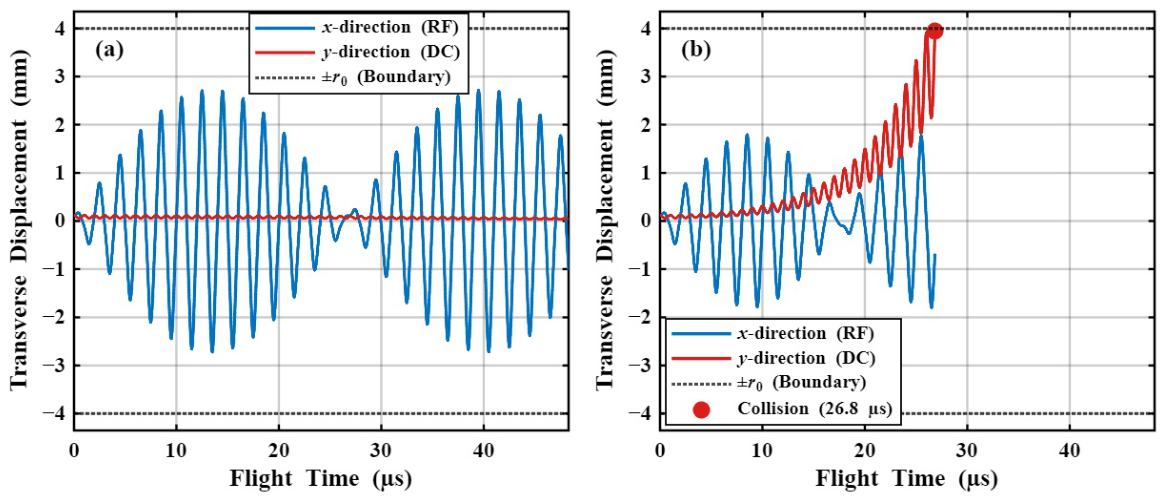
Figure 2 compares calculated transverse trajectories under resonant and detuned conditions. At resonance ($\Delta f=0$), ions exhibit stable trajectories composed of low-frequency secular motion and RF micromotion, successfully traversing the analyzer (Figure 2a). Conversely, according to the sensitivity relationship in Equation (11), an uncompensated frequency offset of $\Delta f=250$ Hz produces a parameter shift that is amplified by resonant voltage attenuation. Near the stability apex, this shift moves the operating point across the boundary (${\beta }_y\to 0$), leading to trajectory divergence in the y-direction and collision with the electrode at $t\approx 26.8\mathsf{\mu }\mathrm{s}$ (Figure 2b).

Figure 2. Numerically simulated transverse ion trajectories (x- and y-directions) near the apex of the first stability region ($m/z=100$, $r_0=4$ mm, $f_0=1.0$ MHz) for a representative test ion ($x_0=y_0=0.12$ mm, $v_{x0}=v_{y0}=0$, ${\xi }_0=0$): (a) bounded stable trajectory at the nominal resonant frequency; (b) trajectory divergence and electrode collision induced by a frequency offset of $\Delta f=250$ Hz.

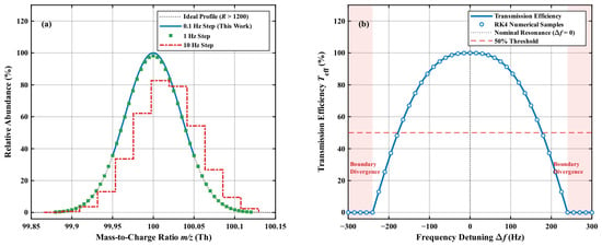
To evaluate the impact of discrete frequency quantization in frequency-scanned operation, Figure 3 shows the resulting mass peak profiles and transmission boundaries around $m/z=100$. As shown in Figure 3b, where circular markers denote discrete RK4 integration samples, the transmission response is governed by the stability apex acceptance and the high-Q resonant attenuation, which restricts the 50% transmission passband to $|\Delta f|\le 150\mathrm{Hz}$ and induces complete trajectory divergence for $|\Delta f|>240\mathrm{Hz}$. When sampling this profile with a 10 Hz step size (Figure 3a), grid mismatch causes discretization artifacts and an apex truncation error of approximately 15.5%, alongside a slight centroid shift. A 1 Hz stepping interval reduces profile distortion, but discrete steps remain visible near the apex. In contrast, a 0.1 Hz frequency step size provides fine parameter tracking, capturing the peak maximum with an amplitude uncertainty below 0.1% and maintaining a symmetric profile with a mass resolving power R defined as [6,11]:

$$R={\displaystyle \frac{m}{\Delta m_{\mathrm{FWHM}}}}>1200$$

(14)

where m is the nominal ion mass (or mass-to-charge ratio $m/z$ for singly charged ions, with $m/z=100\mathrm{Th}$ in this simulation) and $\Delta m_{\mathrm{FWHM}}$ is the peak full width at half maximum. These numerical results indicate that sub-Hertz frequency stepping reduces quantization-induced peak distortion and preserves spectral symmetry in high-resolution frequency-scanned operation.

Figure 3. Coupled RK4–RLC numerical simulations of mass peak quantization and resonant transmission characteristics ($m/z=100\mathrm{Th}$, $f_0=1.0\mathrm{MHz}$, $Q=200$): (a) reconstructed mass peak profiles under 10 Hz, 1 Hz, and 0.1 Hz frequency tuning increments; (b) normalized ion transmission efficiency $T_{\mathrm{eff}}$ versus driving frequency detuning $\Delta f$.

2.3. High-Q Series RLC Resonant Network and Detuning Attenuation Model

To generate high-voltage sinusoidal RF potentials from low-voltage sources with low power dissipation, a series RLC resonant circuit is commonly used as a passive step-up stage [13,15]. The equivalent lumped circuit consists of the power amplifier output resistance $R_{\mathrm{s}}$, the tuning inductor L with series resistance $R_{\mathrm{L}}$, and the total load capacitance $C_{\mathrm{total}}=C_{\mathrm{quad}}+C_{\mathrm{cable}}+C_{\mathrm{stray}}$, where $C_{\mathrm{quad}}$ is the inter-electrode capacitance of the quadrupole analyzer [14].

The continuous-time transfer function $H\left(s\right)=V_{\mathrm{out}}\left(s\right)/V_{\mathrm{in}}\left(s\right)$ in the Laplace domain is expressed as:

$$H\left(s\right)={\displaystyle \frac{\frac{1}{s{C}_{\mathrm{total}}}}{R_{\mathrm{eq}}+sL+\frac{1}{s{C}_{\mathrm{total}}}}}={\displaystyle \frac{{\omega }_0^2}{s^2+{\displaystyle \frac{{\omega }_0}{Q}}s+{\omega }_0^2}}$$

(15)

where $R_{\mathrm{eq}}=R_{\mathrm{s}}+R_{\mathrm{L}}$, ${\omega }_0=2\pi f_{\mathrm{res}}=1/\sqrt{L{C}_{\mathrm{total}}}$ is the undamped resonant angular frequency, and Q is the loaded quality factor:

$$Q={\displaystyle \frac{{\omega }_{0}L}{R_{\mathrm{eq}}}}={\displaystyle \frac{1}{{\omega }_0{R}_{\mathrm{eq}}{C}_{\mathrm{total}}}}$$

(16)

Evaluating Equation (15) along the imaginary axis ($s=j\omega$) for a high-Q system ($Q\ge 100$) near resonance ($\omega \approx {\omega }_0$) gives the magnitude response $\left|H\right(\omega \left)\right|$ and phase response $\theta \left(\omega \right)$ [17]:

$$\left|H\left(\omega \right)\right|\approx {\displaystyle \frac{Q}{\sqrt{1+Q^2{\left({\displaystyle \frac{\omega }{{\omega }_0}}-{\displaystyle \frac{{\omega }_0}{\omega }}\right)}^2}}}$$

(17)

$$\theta \left(\omega \right)\approx -\arctan \left[Q\left({\displaystyle \frac{\omega }{{\omega }_0}}-{\displaystyle \frac{{\omega }_0}{\omega }}\right)\right]$$

(18)

where $\theta \left(\omega \right)$ represents the phase deviation relative to the nominal $-{90}^{\circ }$ phase shift at resonance. At resonance ($\omega ={\omega }_0$), the network provides a voltage gain of $\left|H\right({\omega }_0\left)\right|=Q$ with zero detuning phase offset ($\theta =0$).

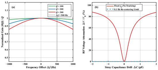
In quadrupole driving systems, loaded quality factors ($Q\in [100,250]$) are chosen to provide passive voltage gain while attenuating higher harmonics. However, a higher Q-factor narrows the $3\mathrm{dB}$ passband ($\mathrm{BW}=f_{\mathrm{res}}/Q$) [14]. As shown in Figure 4a for $Q=200$ and $f_{\mathrm{res}}=1.0\mathrm{MHz}$, the $3\mathrm{dB}$ bandwidth is $5\mathrm{kHz}$. Environmental temperature gradients and mechanical changes cause drifts in the total load capacitance $\Delta C_{\mathrm{total}}$, shifting the resonant frequency according to:

$${\displaystyle \frac{\Delta f_{\mathrm{res}}}{f_{\mathrm{res}}}}={\displaystyle \frac{1}{\sqrt{1+{\displaystyle \frac{\Delta C_{\mathrm{total}}}{C_{\mathrm{total}}}}}}}-1\approx -{\displaystyle \frac{1}{2}}{\displaystyle \frac{\Delta C_{\mathrm{total}}}{C_{\mathrm{total}}}}$$

(19)

As shown in Figure 4b, a capacitive drift of $\Delta C=0.5\mathrm{pF}$ on a $C_{\mathrm{total}}=50\mathrm{pF}$ load produces a resonant frequency shift of approximately $5\mathrm{kHz}$. Operating near the edge of the passband induces phase deviations $\left|\theta \right|>{45}^{\circ }$ and voltage attenuation exceeding $50\%$. Even a frequency offset of $\Delta f=500\mathrm{Hz}$ produces a phase shift of $\theta \approx -11.3^{\circ }$ and a voltage attenuation of $1.9\%$, which shifts the operating line $a/q=2U/V$.

Figure 4. Frequency response and detuning characteristics of the series high-Q RLC resonant network: (a) normalized voltage gain $\left|H\right(f\left)\right|/Q$ versus frequency offset $\Delta f$ for quality factors $Q=100,200,$ and 300, where the dotted vertical line indicates a $\Delta f=500$ Hz offset producing a 1.9% voltage attenuation ($Q=200$); (b) RF voltage attenuation resulting from load capacitance drift $\Delta C$ ($C_0=50$ pF), showing that 0.1 Hz frequency adjustment bounds residual detuning attenuation to below ${10}^{-5}$.

To restore the operational point to the resonance peak following capacitive drift, frequency re-centering requires fine frequency resolution. While 1 Hz stepping can approximate the passband center, residual offsets can lead to phase errors in high-Q networks. A 0.1 Hz frequency resolution provides a relative adjustment step of $\Delta f/f_{\mathrm{res}}\le {10}^{-7}$ at $1.0\mathrm{MHz}$, restricting theoretical detuning-induced voltage attenuation to $\Delta V/V_0<{10}^{-5}$ and maintaining amplitude stability for the resonant load.

3. System Architecture and Hardware Implementation

3.1. System Architecture Overview

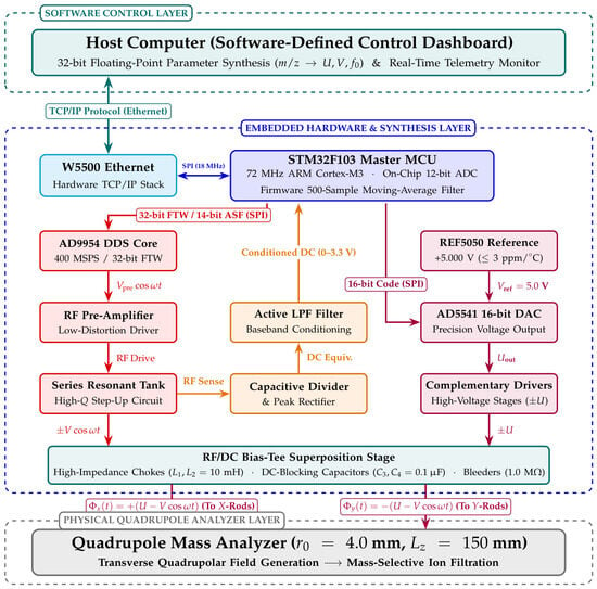
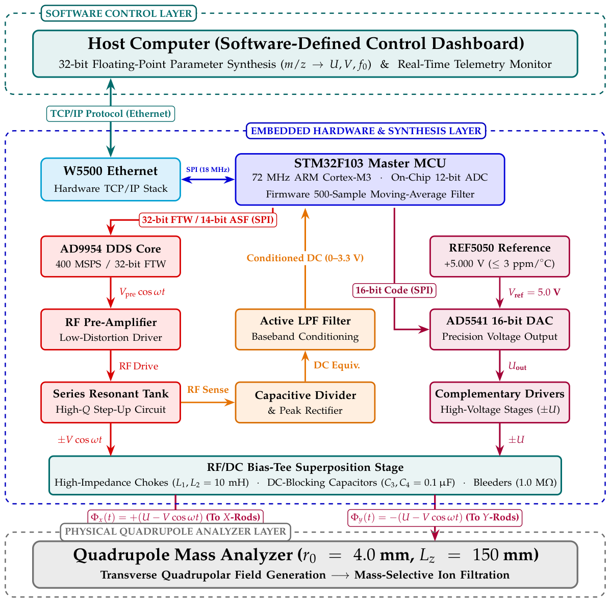
The architecture of the software-defined RF/DC driver is shown in Figure 5. The system comprises a host software interface, a W5500 Ethernet controller, an STM32F103 master microcontroller (ARM Cortex-M3 core, 72 MHz), an AD9954 Direct Digital Synthesis (DDS) core (400 MSPS) [25], an RF pre-amplifier coupled to a series resonant tank, a 16-bit bipolar DC bias circuit [26], and an in-loop baseband telemetry channel [27].

Figure 5. Block diagram of the software-defined RF/DC driver architecture, showing the digital synthesis, DC bias generation, RF/DC superposition, and amplitude telemetry stages. (Note: The physical quadrupole load was modeled and simulated in Section 2 and represented by an equivalent 50 pF capacitive load during benchtop characterization).

Target operational parameters (U, V, and $f_0$) are calculated by the host software. Control commands are encapsulated into TCP/IP frames and transmitted over Ethernet. The microcontroller parses the payload, updates the internal registers of the DDS and DAC via Serial Peripheral Interface (SPI) buses, and manages output synchronization. The synthesized RF carrier is amplified and coupled into the series resonant tank to generate the required RF potential. Simultaneously, the amplitude telemetry channel rectifies and filters the resonant tank voltage, which is then digitized by the microcontroller’s internal ADC and returned to the host for monitoring.

3.2. DDS Core and Sub-Hertz Frequency Configuration

The RF sinusoidal signal is digitally synthesized by an AD9954 DDS core featuring a 32-bit phase accumulator, an on-chip 14-bit DAC, and a system clock frequency of $f_c=400\mathrm{MHz}$ [22,25]. In single-tone continuous-wave mode, the synthesized output frequency $f_0$ is determined by the 32-bit Frequency Tuning Word (FTW, denoted by K) and the clock frequency $f_c$ [21,23]:

$$f_0={\displaystyle \frac{K·f_c}{2^N}}={\displaystyle \frac{K·f_c}{2^{32}}}$$

(20)

The corresponding integer FTW is calculated by:

$$K=\mathrm{round}\left({\displaystyle \frac{f_0·2^{32}}{f_c}}\right)$$

(21)

For $f_c=400\mathrm{MHz}$, the intrinsic frequency resolution of the 32-bit accumulator is $\Delta f_{\mathrm{intrinsic}}=400\mathrm{MHz}/2^{32}\approx 0.0931\mathrm{Hz}<0.1\mathrm{Hz}$. In many embedded implementations, target frequencies are transmitted as integer values in hertz or kilohertz, which truncates fractional frequencies. In this design, the host and microcontroller exchange target frequencies using the IEEE-754 32-bit single-precision floating-point format. This allows setpoints with 0.1 Hz resolution to be directly mapped into the 32-bit FTW via Equation (21) without integer truncation.

The RF output amplitude is scaled by the 14-bit Amplitude Scale Factor (ASF, denoted by A) in the Amplitude Control Register (address 0x02) [25]:

$$V_{\mathrm{out}}=V_{\mathrm{FS}}·{\displaystyle \frac{A}{2^{14}}}=V_{\mathrm{FS}}·{\displaystyle \frac{A}{16384}}$$

(22)

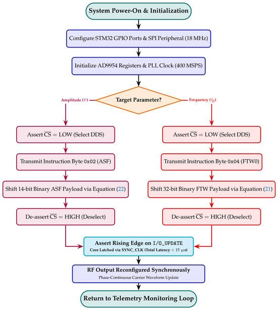
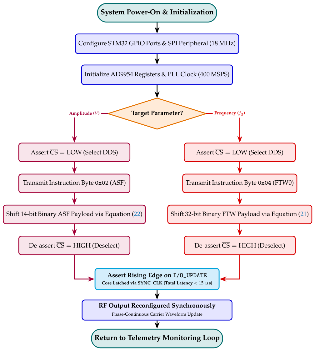
where $V_{\mathrm{FS}}$ is the full-scale pre-amplifier input amplitude ($V_{\mathrm{pre}}$ in Figure 5). As shown in Figure 6, to update either parameter, the microcontroller asserts the chip select line ($\overline{\mathrm{CS}}$), transmits the 8-bit instruction byte via SPI, writes the corresponding payload (32-bit FTW or 14-bit ASF), and de-asserts $\overline{\mathrm{CS}}$. A rising edge is then applied to the I/O_UPDATE pin to synchronously latch the buffered values into the active DDS core registers.

Figure 6. Microcontroller execution timing sequence and register configuration flowchart for AD9954 frequency and amplitude modulation.

3.3. Microcontroller and Ethernet Communication Interface

To provide higher throughput and lower transmission latency than conventional asynchronous serial interfaces (such as UART), an Ethernet communication interface is implemented using a W5500 hardware TCP/IP controller. The host computer operates as a TCP client, while the embedded W5500 is configured as a TCP server.

The STM32F103 microcontroller communicates with the W5500 via an SPI bus at $18\mathrm{MHz}$. Control instructions are formatted into a 9-byte frame comprising a 2-byte preamble (0xAA55), a 1-byte command identifier, a 4-byte IEEE-754 single-precision floating-point payload, and a 2-byte cyclic redundancy check (CRC-16). When a frame is received in the socket buffer, the W5500 asserts an interrupt signal to the microcontroller. The interrupt service routine (ISR) validates the CRC checksum, parses the floating-point payload, and updates the corresponding DDS or DAC registers via SPI. The entire sequence completes within $15\mathsf{\mu }\mathrm{s}$, enabling low-latency parameter reconfiguration.

3.4. DC Bias Generator and RF/DC Bias-Tee Superposition Network

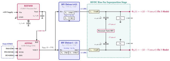
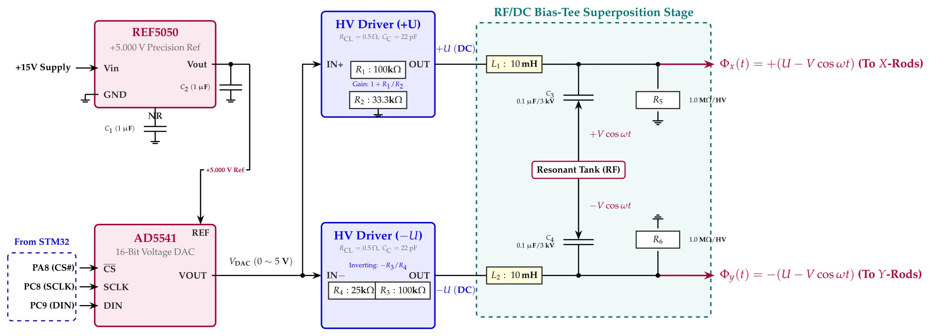
The static DC bias potentials ($\pm U$) that define the operating point in the Mathieu stability diagram require sub-millivolt resolution and low thermal drift. As shown in Figure 7, the DC generation and coupling circuit consists of a precision voltage reference (REF5050), a 16-bit unipolar voltage-output DAC (AD5541), complementary driver stages, and an on-board RF/DC bias-tee superposition network.

Figure 7. Schematic of the 16-bit DC bias generator and RF/DC bias-tee superposition circuit. The circuit includes a voltage reference (REF5050), a 16-bit DAC (AD5541), complementary driver stages, and L–C filtering branches ($L_1,L_2=10\mathrm{mH}$; $C_3,C_4=0.1\mathsf{\mu }\mathrm{F}/3\mathrm{kV}$; $R_5,R_6=1.0\mathrm{M}\mathsf{\Omega }$) that superimpose the RF and DC potentials.

The reference potential is provided by an REF5050 IC powered from a $+15$ V analog supply rail. It supplies a $+5.000$ V output with a temperature coefficient of ≤3 ppm/°C and a low-frequency noise of $3\mathsf{\mu }{\mathrm{V}}_{\mathrm{p}\text{-}\mathrm{p}}/\mathrm{V}$ across the 0.1 to 10 Hz band. A $1.0\mathsf{\mu }\mathrm{F}$ noise-reduction capacitor ($C_1$) is connected to the TRIM/NR pin to filter internal bandgap noise, and the output is decoupled by a ceramic capacitor ($C_2=1.0\mathsf{\mu }\mathrm{F}$). The AD5541 DAC interfaces with the STM32 microcontroller via general-purpose pins PA8 for chip select ($\overline{\mathrm{CS}}$), PC8 for serial clock (SCLK), and PC9 for serial data (DIN). Digital codes are shifted into the internal register, and the analog output is updated on the rising edge of the $\overline{\mathrm{CS}}$ signal.

The analog output voltage of the DAC is given by:

$$U_{\mathrm{out}}=V_{\mathrm{ref}}·{\displaystyle \frac{D_{\mathrm{DAC}}}{2^{16}}}=5.000\mathrm{V}·{\displaystyle \frac{D_{\mathrm{DAC}}}{65536}}$$

(23)

where $D_{\mathrm{DAC}}\in [0,65535]$ is the digital input code. The corresponding theoretical step size is $\Delta U_{\min }=5.000\mathrm{V}/65536\approx 76.29\mathsf{\mu }\mathrm{V}$, providing the target 0.1 mV resolution across the 10 mV to 5 V span.

To drive the quadrupole electrodes while isolating the low-voltage digital circuitry from high RF voltages, the DAC output is routed to complementary driver stages powered by symmetric high-voltage rails ($\pm V_{\mathrm{HV}}$), followed by a bias-tee network. Each driver stage includes external current-limiting resistors ($R_{\mathrm{CL}}=0.5\mathsf{\Omega }$), phase-compensation capacitors ($C_{\mathrm{C}}=22$ pF), and gain-setting feedback resistors: $R_1=100\mathrm{k}\mathsf{\Omega },R_2=33.3\mathrm{k}\mathsf{\Omega }$ (providing a non-inverting gain of $+4.0$) for the positive channel, and $R_3=100\mathrm{k}\mathsf{\Omega },R_4=25\mathrm{k}\mathsf{\Omega }$ (providing an inverting gain of $-4.0$) for the complementary channel. The resulting DC potentials ($\pm U$) are coupled to the output feedlines through high-inductance RF chokes ($L_1,L_2=10\mathrm{mH}$, wound in multi-section pie configurations to minimize parasitic capacitance and ensure self-resonance well above 1.0 MHz), providing an inductive reactance of $X_L=2\pi fL\approx 62.8\mathrm{k}\mathsf{\Omega }$ at 1.0 MHz to block RF signals from entering the DC drivers. Concurrently, the RF potentials ($\pm V\cos \omega t$) are AC-coupled through high-voltage ceramic capacitors ($C_3,C_4=0.1\mathsf{\mu }\mathrm{F}$, rated for 3 kV), while bleeder resistors ($R_5,R_6=1.0\mathrm{M}\mathsf{\Omega }$) provide a DC discharge path with negligible loading on the resonant tank. This bias-tee network superimposes the RF and DC voltages, delivering ${\mathsf{\Phi }}_x\left(t\right)=+(U-V\cos \omega t)$ and ${\mathsf{\Phi }}_y\left(t\right)=-(U-V\cos \omega t)$ to the output terminals while protecting the low-voltage synthesis electronics.

3.5. RF Amplitude Detection and Digital Filtering

To monitor the resonant tank voltage and track detuning, an amplitude detection circuit is connected across the resonant network. The RF voltage is scaled down through a capacitive divider, rectified by a diode peak detector, and smoothed by an active low-pass filter to produce a DC voltage proportional to the RF peak amplitude [27].

This DC voltage is sampled by the 12-bit on-chip ADC of the STM32 microcontroller. To suppress residual RF ripple and 50 Hz power-line noise, a moving-average filter is implemented in firmware [28]. The filtered sensing voltage ${\overline{V}}_{\mathrm{sense}}$ is computed over a sliding buffer of $N_{\mathrm{avg}}=500$ consecutive samples:

$${\overline{V}}_{\mathrm{sense}}={\displaystyle \frac{1}{N_{\mathrm{avg}}}}{\displaystyle \sum _{k=1}^{N_{\mathrm{avg}}}}{V}_{\mathrm{adc}}\left[k\right],(N_{\mathrm{avg}}=500)$$

(24)

Assuming uncorrelated noise with variance ${\sigma }_{\mathrm{noise}}^2$, the variance of the averaged measurement is reduced by a factor of $N_{\mathrm{avg}}$:

$${\sigma }_{\overline{V}}^2={\displaystyle \frac{{\sigma }_{\mathrm{noise}}^2}{N_{\mathrm{avg}}}}={\displaystyle \frac{{\sigma }_{\mathrm{noise}}^2}{500}}$$

(25)

This yields a theoretical signal-to-noise ratio (SNR) improvement of $10{\log }_{10}\left(500\right)\approx 27\mathrm{dB}$, reducing ADC quantization flicker and thermal noise. The resulting telemetry value is transmitted to the host computer via Ethernet.

4. Experimental Results

4.1. Experimental Test Bench Setup and Fabricated Prototype

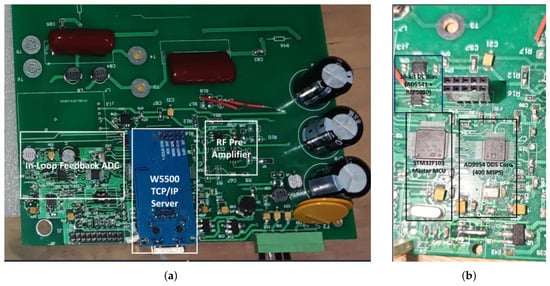
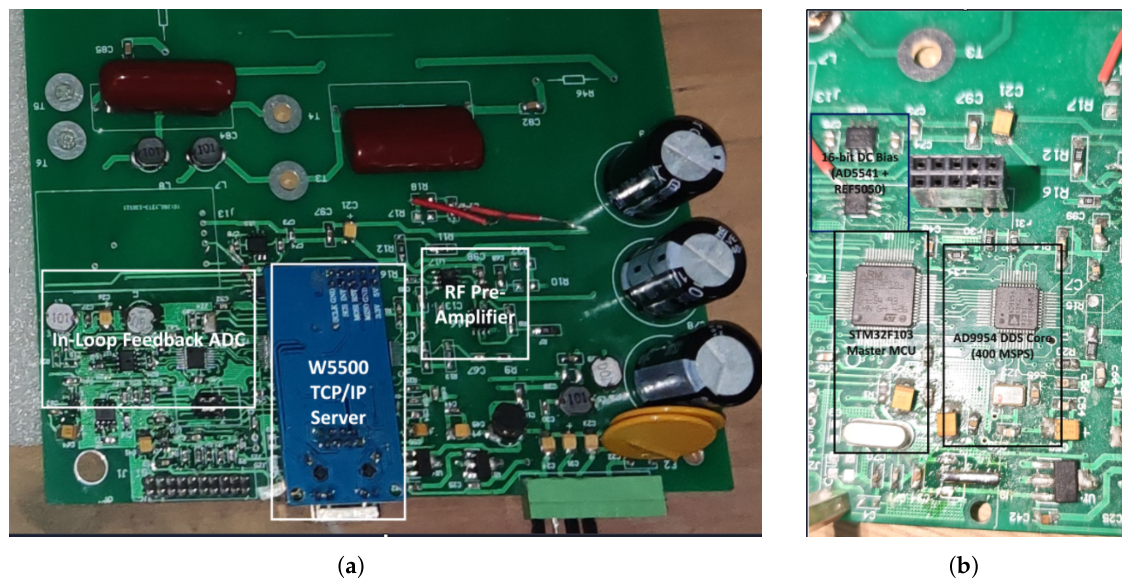
The driver circuit was fabricated on a two-layer PCB and characterized on a benchtop test setup, as shown in Figure 8.

Figure 8. Photographs of the fabricated software-defined RF/DC driver prototype: (a) overview of the PCB showing the W5500 Ethernet module, RF pre-amplifier, amplitude conditioning circuit, and resonant capacitors; (b) close-up of the digital synthesis and DC bias stage, including the STM32F103 microcontroller, AD9954 DDS core (400 MSPS), and AD5541 DAC with REF5050 reference.

The board layout (Figure 8a) contains the W5500 Ethernet controller, an RF pre-amplifier, high-voltage polypropylene resonant capacitors, and the amplitude detection circuitry. The digital core (Figure 8b) consists of the STM32F103 microcontroller, an AD9954 DDS clocked by a local crystal oscillator, and an AD5541 16-bit DAC with an REF5050 ($+5.000\mathrm{V}$) voltage reference.

The board interfaces with a host PC over Ethernet using TCP/IP sockets for register configuration and telemetry data logging. Output waveforms, frequency stepping, and stability were captured with a digital storage oscilloscope (RIGOL DS4052, 500 MHz, 4 GSa/s) using 10:1 passive probes ($10\mathrm{M}\mathsf{\Omega }\Vert 10\mathrm{pF}$). To replicate the 1.0 MHz series resonant tank and the capacitive loading of a quadrupole rod assembly, a 507 $\mathsf{\mu }$H tuning inductor ($R_{\mathrm{eq}}\approx 15.9\mathsf{\Omega }$) was connected to a 50 pF capacitive load, setting the loaded quality factor to $Q\approx 200$. DC bias voltages were recorded with a digital multimeter (VICTOR VC890C+).

4.2. Sub-Hertz Frequency Granularity and Wideband Synthesis Performance

To verify that the communication pipeline and firmware preserve fractional frequency resolution, consecutive target setpoints with a 0.1 Hz step ($f_{\mathrm{target}1}=100.5$ Hz and $f_{\mathrm{target}2}=100.6$ Hz) were commanded from the host software. Because the AD9954 DDS core operates from a clock frequency of $f_c=400$ MHz with a 32-bit phase accumulator, its intrinsic tuning resolution is:

$$\Delta f_{\mathrm{intrinsic}}={\displaystyle \frac{f_c}{2^{32}}}={\displaystyle \frac{400\mathrm{MHz}}{2^{32}}}\approx 0.09313\mathrm{Hz}<0.1\mathrm{Hz}$$

(26)

A 100 Hz carrier was selected for step verification because the internal 6-digit reciprocal frequency counter of the oscilloscope (RIGOL DS4052) provides a 1 mHz resolution near 100 Hz, whereas at 1 MHz its readout resolution is limited to 1 Hz. Setting target frequencies of $f_{\mathrm{target}1}=100.5$ Hz and $f_{\mathrm{target}2}=100.6$ Hz updates the 32-bit Frequency Tuning Word from $K_1=\mathrm{1,079,110}$ to $K_2=\mathrm{1,080,184}$ via Equation (21). This digital increment of $\Delta K=1074$ corresponds to an intended frequency step of $\Delta f_{\mathrm{DDS}}=1074\times (400\mathrm{MHz}/2^{32})\approx 0.10002$ Hz. The measured output frequencies shifted from 100.489 Hz to 100.575 Hz, giving a measured step of $\Delta f_{\mathrm{meas}}\approx 0.086$ Hz. The difference of approximately 14 mHz between the measured and theoretical step falls within the counter measurement uncertainty caused by trigger noise and single-count gating limits. Because integer-truncated parsing would result in either zero change ($\Delta K=0$) or a 1 Hz step ($\Delta K\approx \mathrm{10,737}$), the measured step confirms that the floating-point protocol and firmware maintain sub-Hertz resolution without integer truncation. By the linear DDS tuning relation in Equation (20), this frequency step resolution is maintained across the operating band. Specifically, at the nominal operating frequency of $f_0=1.0\mathrm{MHz}$ ($2^{19}<f_0<2^{20}$), the 24-bit mantissa of the IEEE-754 single-precision format provides a unit-in-the-last-place (ULP) resolution of $2^{19}/2^{23}=0.0625\mathrm{Hz}<0.1\mathrm{Hz}$, ensuring that $0.1\mathrm{Hz}$ command increments are represented without floating-point rounding loss. Commanding a $0.1\mathrm{Hz}$ step from $\mathrm{1,000,000.0}\mathrm{Hz}$ to $\mathrm{1,000,000.1}\mathrm{Hz}$ deterministically increments the 32-bit FTW register from $K_1=\mathrm{10,737,418}$ to $K_2=\mathrm{10,737,419}$ ($\Delta K=1\mathrm{LSB}$, yielding $\Delta f_{\mathrm{DDS}}=0.09313\mathrm{Hz}$). Because the synchronous 32-bit phase accumulator hardware adds $\Delta K$ identically per $400\mathrm{MHz}$ clock cycle regardless of the base word $K_1$, the incremental step size is invariant to carrier frequency, while the carrier stability at $1.0\mathrm{MHz}$ is governed by the local crystal oscillator tolerance characterized in Table 1.

Table 1. Measured frequency synthesis accuracy across six decade intervals.

Target Frequency (${\mathit{f}}_{\mathbf{target}}$)	Measured Frequency (${\mathit{f}}_{\mathbf{meas}}$)	Relative Error (${\mathit{\delta }}_{\mathit{f}}$)
$10\mathrm{Hz}$	$9.997\mathrm{Hz}$	$0.030\%$
$100\mathrm{Hz}$	$99.978\mathrm{Hz}$	$0.022\%$
$1\mathrm{kHz}$	$999.960\mathrm{Hz}$	$0.004\%$
$10\mathrm{kHz}$	$9.998\mathrm{kHz}$	$0.020\%$
$100\mathrm{kHz}$	$100.001\mathrm{kHz}$	$0.001\%$
$1\mathrm{MHz}$	$999.300\mathrm{kHz}$	$0.070\%$
$10\mathrm{MHz}$	$10.0001\mathrm{MHz}$	$0.001\%$

From Equation (10), at $f_0=1.0\mathrm{MHz}$, a 0.1 Hz step restricts the relative parameter shift to $|\Delta q/q|<2\times {10}^{-7}$, avoiding shifts across the stability boundary near the apex as modeled in Section 2.2.

The wideband frequency synthesis accuracy was measured at the RF pre-amplifier output from 10 Hz to 10 MHz in decade steps. As summarized in Table 1, the relative frequency error ${\delta }_f=|f_{\mathrm{meas}}-f_{\mathrm{target}}|/f_{\mathrm{target}}\times 100\%$ remains below $0.070\%$ across the measured range. At 1 MHz, the measured frequency of 999.300 kHz represents a relative offset of 0.070% ($700\mathrm{Hz}$). It is important to distinguish between absolute frequency accuracy and differential frequency resolution in this architecture. The $0.070\%$ static offset reflects absolute frequency accuracy, which is primarily due to on-board crystal oscillator tolerance and counter gate-time limitations; this static offset can be compensated via a single-point software calibration factor or an external reference clock. In contrast, the $0.1\mathrm{Hz}$ specification represents differential frequency resolution (tuning granularity, $\Delta f_{\mathrm{intrinsic}}=f_c/2^{32}\approx 0.0931\mathrm{Hz}$), which is strictly monotonic and governed by the 32-bit phase accumulator. For dynamic resonance tracking, differential resolution rather than absolute crystal accuracy is the governing parameter, because the physical resonant frequency $f_{\mathrm{res}}$ of a high-Q tank inherently shifts by several kilohertz due to parasitic capacitance tolerances and thermal drift. Across the linear range of the pre-amplifier, the output amplitude is adjustable from $3.8{\mathrm{V}}_{\mathrm{p}\text{-}\mathrm{p}}$ to $18.9{\mathrm{V}}_{\mathrm{p}\text{-}\mathrm{p}}$. The total harmonic distortion (THD) of the pre-amplifier output is below $-42\mathrm{dBc}$ (dominated by the second harmonic) prior to bandpass filtering by the series resonant tank. When coupled to the $1.0\mathrm{MHz}$ series RLC resonant tank ($L=507\mathsf{\mu }\mathrm{H}$, $50\mathrm{pF}$ capacitive load, $Q\approx 200$), passive resonant step-up yields a maximum undistorted RF voltage of $890{\mathrm{V}}_{\mathrm{p}\text{-}\mathrm{p}}$ (≈445 V zero-to-peak, corresponding to the $4.450\mathrm{V}$ full-scale peak-detector output scaled through a 100:1 capacitive divider ratio in Section 4.3) across the $50\mathrm{pF}$ load.

To evaluate the baseline thermal drift of the high-Q resonant tank and quantify the detuning that must be compensated, open-loop power-cycling measurements were conducted on the loaded RLC circuit ($f_{\mathrm{res}}\approx 1.0\mathrm{MHz}$) over a 60-min interval ($n=7$ independent trials). The Relative Standard Deviation (RSD) of the loaded resonant frequency is calculated as:

$$\mathrm{RSD}={\displaystyle \frac{S}{\overline{x}}}\times 100\%={\displaystyle \frac{1}{\overline{x}}}\sqrt{{\displaystyle \frac{1}{n-1}}\sum _{i=1}^n{(x_i-\overline{x})}^2}\times 100\%$$

(27)

Thermal drift in the tuning inductor and load capacitance resulted in an open-loop resonant frequency variation of $\mathrm{RSD}=2.66\times {10}^{-3}$ (0.266%, corresponding to a characteristic thermal drift of ≈2.66 kHz over a 60-min cycle). Because this multi-kilohertz thermal drift substantially exceeds the 50% transmission passband ($|\Delta f|\le 150\mathrm{Hz}$) and the stability boundary ($\Delta f\le 250\mathrm{Hz}$) identified in Section 2.2, it experimentally demonstrates the necessity of sub-Hertz frequency tuning to re-center the driving carrier onto the shifted resonance peak.

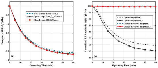
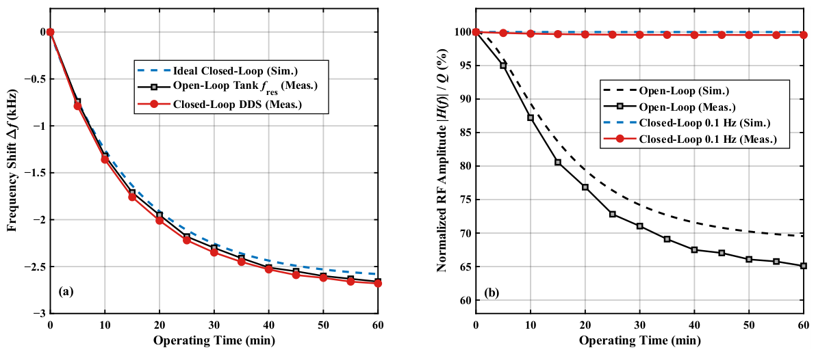
To validate closed-loop resonance re-centering and compare experimental tracking performance against theoretical predictions from Equations (17) and (19), comparative 60-min warm-up tests (an open-loop fixed-carrier run using brief millisecond-scale sweep probes at 5-min intervals to log $f_{\mathrm{res}}\left(t\right)$, followed by a cooled-down closed-loop tracking run) were conducted alongside coupled numerical simulations, as shown in Figure 9. In the proposed resonance-tracking architecture, the series RLC transfer function $\left|H\right(f_0\left)\right|$ exhibits a unimodal maximum around the instantaneous loaded resonant frequency $f_{\mathrm{res}}\left(t\right)$, where the rectified telemetry voltage ${\overline{V}}_{\mathrm{sense}}$ reaches its global apex ($\partial {\overline{V}}_{\mathrm{sense}}/\partial f_0=0$). Using a perturb-and-observe (hill-climbing) extremum-seeking routine, the controller applies incremental frequency perturbations ($\Delta f_{\mathrm{step}}$ in $0.1\mathrm{Hz}$ resolution), evaluates the sign of the telemetry gradient $\Delta {\overline{V}}_{\mathrm{sense}}/\Delta f_0$ after the $5\mathrm{ms}$ moving-average filter settling window, and iteratively steps the DDS carrier toward the shifted resonance apex. Combining the measured telemetry noise floor ($\mathrm{RSD}=1.2\times {10}^{-5}$ in Section 4.3) with the parabolic passband curvature of Equation (17) near resonance ($\Delta V/V_0\approx -2Q^2{(\Delta f/f_{\mathrm{res}})}^2$), the minimum frequency offset at which resonant attenuation exceeds the $3\sigma$ telemetry noise threshold ($3.6\times {10}^{-5}$) for $Q=200$ is $|\Delta f_{\min }|=f_{\mathrm{res}}\sqrt{3.6\times {10}^{-5}/\left(2Q^2\right)}\approx 0.42\mathrm{Hz}$. Because the DDS stage provides a deterministic $0.1\mathrm{Hz}$ tuning step ($\Delta f_{\mathrm{DDS}}<|\Delta f_{\min }|$), the hardware loop provides sufficient resolution and signal-to-noise margin to bound steady-state resonant amplitude deviations below $3.6\times {10}^{-5}$ (excluding slow inductor copper-loss variations).

Figure 9. Simulated and experimentally measured closed-loop resonance tracking performance over a 60-min thermal drift cycle ($f_{\mathrm{res}0}=1.0\mathrm{MHz}$, $Q\approx 200$, $50\mathrm{pF}$ load): (a) simulated ideal tracking trajectory compared against the measured open-loop tank resonant drift $f_{\mathrm{res}}$ and closed-loop DDS carrier tracking trajectory; (b) normalized RF output amplitude $\left|H\right(f\left)\right|/Q$ comparing open-loop fixed-frequency operation against closed-loop $0.1\mathrm{Hz}$ tracking.

As shown in Figure 9a, during the 60-min warm-up period, the open-loop tank resonant frequency $f_{\mathrm{res}}$ drifted by $-2.66\mathrm{kHz}$ (closely following the $-2.60\mathrm{kHz}$ theoretical exponential thermal model), while the closed-loop DDS carrier accurately tracked the thermal shift to $-2.68\mathrm{kHz}$ (reflecting slightly higher continuous resonant self-heating in the inductor under full-power closed-loop excitation). Consequently, as shown in Figure 9b, whereas open-loop operation at a fixed $1.0\mathrm{MHz}$ carrier suffered a $34.9\%$ amplitude drop (falling to $65.1\%$, slightly below the $69.5\%$ ideal curve due to thermal resistance increases in the inductor winding), closed-loop $0.1\mathrm{Hz}$ tracking maintained the normalized RF output amplitude within $99.55\%$ to $100.00\%$ across the entire 60-min thermal cycle.

4.3. Telemetry Acquisition Noise Floor and Filter Stability Evaluation

To evaluate the electronic noise floor and filtering performance of the telemetry acquisition path independently of RF power fluctuations, a precision DC voltage source ($V_{\mathrm{in}}=4.450$ V) was applied to the analog conditioning circuit. This input corresponds to a typical peak-detector output near the upper limit of the measurement range. Because the 12-bit on-chip ADC operates across an input span of 0 to 3.3 V, an active scaling buffer attenuates the input with a scaling ratio of $k_{\mathrm{div}}=0.60$, mapping the 4.450 V input to approximately 2.67 V to avoid ADC rail clipping. The microcontroller firmware then scales the digitized value back to the input voltage level using the inverse attenuation coefficient.

Over a 60-min duration, the 500-sample moving-average filter was executed in firmware, and telemetry values were recorded over Ethernet at 5-min intervals, as summarized in Table 2.

Table 2. Measured telemetry voltages and stability of the ADC channel with a 500-sample moving-average filter ($V_{\mathrm{in}}=4.450$ V).

Sampling Time (min)	Telemetry Voltage (V)	Relative Offset (${\mathit{\delta }}_{\mathbf{sense}}$)
0	4.4529	0.0652%
5	4.4529	0.0652%
10	4.4529	0.0652%
15	4.4529	0.0652%
20	4.4529	0.0652%
25	4.4530	0.0674%
30	4.4530	0.0674%
35	4.4530	0.0674%
40	4.4530	0.0674%
45	4.4530	0.0674%
50	4.4530	0.0674%
55	4.4529	0.0652%
60	4.4529	0.0652%

Throughout the 60-min test, the reconstructed telemetry potential remained between 4.4529 V and 4.4530 V, showing a static offset below 0.0674% and a relative standard deviation (RSD) of $1.2\times {10}^{-5}$. This result agrees with the theoretical noise attenuation in Equation (25), confirming that the 500-sample moving-average filter suppresses random electronic noise and ADC quantization flicker by approximately 27 dB.

In RF operation, the resonant voltage is scaled by a capacitive divider and envelope-detected by a Schottky diode peak detector. While the DC test above benchmarks the stability of the active buffer and ADC stages ($\mathrm{RSD}=1.2\times {10}^{-5}$, corresponding to ≈53.4$\mathsf{\mu }\mathrm{V}$ rms at $4.450\mathrm{V}$), the forward voltage drop ($V_F$) of the rectifier diode varies with temperature at a typical rate of $\partial V_F/\partial T\approx -1.5\mathrm{to}-2.0\mathrm{mV}{/}^{\circ }\mathrm{C}$. Relative to the $4.450\mathrm{V}$ nominal envelope output, an uncompensated $1 °\mathrm{C}$ ambient temperature change induces a relative voltage shift of $3.4\times {10}^{-4}\mathrm{to}4.5\times {10}^{-4}{/}^{\circ }\mathrm{C}$ ($0.034\%\text{–}0.045\%{/}^{\circ }\mathrm{C}$), which is approximately $28\mathrm{to}37$ times larger than the intrinsic ADC acquisition RSD of $1.2\times {10}^{-5}$. However, because resonance frequency tracking locates the relative amplitude maximum ($\partial {\overline{V}}_{\mathrm{sense}}/\partial f_0=0$) over millisecond-scale perturbation intervals during which the diode temperature is quasi-static, slow thermal drift in $V_F$ does not shift the identified resonant frequency $f_{\mathrm{res}}$. In practical implementations requiring absolute amplitude regulation across wide ambient temperatures, this diode thermal drift can be compensated in firmware using an on-board temperature sensor and a calibrated look-up table (LUT).

4.4. DC Bias Output Linearity and Resolution Verification

The DC bias generation stage was evaluated for output linearity and step resolution. Test setpoints were commanded from the host software: a small-signal setpoint of 10 mV and five points from 1000 mV to 5000 mV at 1000 mV intervals.

As shown in Table 3, the output voltage increases monotonically from 10 mV to 5.00 V across the DAC output span. These measurements benchmark the core digital-to-analog conversion at the DAC output pin ($V_{\mathrm{DAC}}$). To verify the subsequent high-voltage stage, the complementary outputs ($\pm U$) following the $\pm 4.0$-gain driver circuits were evaluated across the corresponding $\pm 0.04\mathrm{V}$ to $\pm 20.00\mathrm{V}$ range. Due to the high open-loop gain and low input offset of the operational amplifiers (OPA2277), the output offset voltage remained below $\pm 0.5\mathrm{mV}$, and the gain matching error between the complementary rails was within $\pm 0.15\%$. No saturation or nonlinear clipping was observed across the operational range, confirming that symmetrical bipolar DC bias is preserved for the quadrupole electrodes.

Table 3. Target and measured DC bias voltages across the output range.

Target Voltage (mV)	10	1000	2000	3000	4000	5000
Measured Voltage	10.0 mV	1.00 V	2.00 V	3.00 V	4.00 V	5.00 V

The 0.1 mV stepping resolution is supported by the 16-bit resolution of the AD5541 DAC. Operating with the $+5.000$ V reference (REF5050), the theoretical step size is:

$$\Delta U_{\min }={\displaystyle \frac{V_{\mathrm{ref}}}{2^{16}}}={\displaystyle \frac{5.000\mathrm{V}}{65536}}\approx 76.29\mathsf{\mu }\mathrm{V}<0.1\mathrm{mV}$$

(28)

Because the AD5541 guarantees monotonic behavior with differential non-linearity $\mathrm{DNL}\le \pm 0.5$ LSB, the circuit avoids missing codes. In addition, the low temperature drift of the voltage reference (≤3 ppm/°C) and the low-offset operational amplifier buffer (OPA2277) maintain setpoint stability across operating temperatures.

5. Discussion

5.1. Comparison with Reported Quadrupole Drivers

Table 4 summarizes the specifications of the proposed circuit alongside representative quadrupole and multipole driving systems reported in the literature.

Table 4. Comparison with representative quadrupole RF/DC driving systems.

Parameter/Feature	O’Connor et al. [16]	Schaefer et al. [17]	Shinholt et al. [19]	This Work
Synthesis Architecture	Manual Inductive Tap	Digital RF Synthesis	Square-Wave Driver	Software-Defined DDS
Control Interface	Manual Tuning	Microcontroller SPI	Standalone Controller	Host Interface (TCP/IP Ethernet)
Frequency Resolution	Fixed/Manual	$1000\mathrm{Hz}$	$1\mathrm{Hz}$	$0.1\mathrm{Hz}$
RF Range	$1.36\mathrm{MHz}$	$1.882\mathrm{MHz}$	$0.2\text{–}1.5\mathrm{MHz}$	$10\mathrm{Hz}\text{–}10\mathrm{MHz}$ *
Frequency Relative Error	$0.09\%$	$0.12\%$	≈0.10%	≤0.070%
Amplitude Resolution	Manual Variac	14-bit DAC	Pulse-Width Modulation	14-bit ASF (16,384 levels)
DC Bias Source	External Power Supply	External Power Supply	External Power Module	Integrated 16-bit DAC (0.1 mV step)
Amplitude Telemetry	None	External Diode	None	On-board 12-bit ADC + Moving Average

* Note: 10 Hz to 10 MHz represents the synthesis range of the DDS pre-amplifier stage; resonant step-up operation was characterized at 1.0 MHz.

Early quadrupole power supplies relied on manual inductor taps or variable capacitors [16], which precluded electronic frequency adjustments during operation. Subsequent digital designs by Schaefer et al. [17] and Shinholt et al. [19] adopted digital synthesis methods; however, their step sizes were constrained to 1000 Hz and 1 Hz, respectively, due to integer parameter parsing or clock divider limits. Compared with these existing DDS-based implementations, the novelty of the proposed RF/DC driver lies in three key aspects: (1) Sub-Hertz Command Granularity: Transmitting IEEE-754 32-bit floating-point frequency commands over Ethernet directly maps setpoints to the 32-bit DDS phase accumulator registers without integer truncation, improving the effective frequency stepping resolution by one to four orders of magnitude ($0.1\mathrm{Hz}$ versus $1\text{–}1000\mathrm{Hz}$ in [17,19]). (2) Wideband Synthesis Accuracy: This implementation achieves 0.1 Hz frequency resolution across six frequency decades (10 Hz to 10 MHz) with a relative error below 0.070%, improving upon the narrower bandwidths (<2 MHz) and $0.09\text{–}0.12\%$ errors reported in prior drivers [16,17,18,19]. (3) Unified Control and Telemetry Capability: Whereas previous designs rely on external DC power supplies and lack integrated feedback [16,18,19], our platform co-integrates sub-Hertz DDS synthesis, a 16-bit bipolar DC bias stage ($0.1\mathrm{mV}$ step resolution), and an on-board amplitude telemetry channel ($\mathrm{RSD}=1.2\times {10}^{-5}$) on a single networked platform (<15$\mathsf{\mu }\mathrm{s}$ command latency) to support automated resonance re-centering.

5.2. Operational Modes and Mass Calibration Considerations

The practical utility of sub-Hertz frequency tuning depends on the operational regime of the quadrupole system.

In conventional voltage-scanning operation, the excitation frequency $f_0$ is held constant, and mass separation is achieved by ramping U and V along a constant ratio line $a/q=2U/V$. Because the transmitted mass-to-charge ratio is inversely proportional to the square of the frequency ($m\propto V/f_0^2$), shifting $f_0$ during an analytical scan directly alters the mass calibration. In this mode, the 0.1 Hz frequency resolution is applied prior to analytical scans as a pre-scan alignment step. For a loaded series RLC tank with $Q=200$ and $f_0=1.0\mathrm{MHz}$ (passband bandwidth of 5 kHz), tuning the carrier frequency to within 0.1 Hz of the tank resonance ($\Delta f/f_0\le {10}^{-7}$) minimizes the initial phase error and maximizes voltage step-up without shifting the mass calibration axis.

In frequency-scanned mass spectrometry (FSMS) [19], mass spectra are acquired by sweeping the carrier frequency across the stability diagram while keeping U and V constant or scaled. In this regime, the frequency step size determines the mass sampling interval. As demonstrated by the numerical simulations in Figure 3, a coarse 10 Hz step size leads to sampling grid mismatch and apex truncation errors of approximately 15.5%. While a 1 Hz increment reduces distortion, discrete steps remain visible near the apex. A 0.1 Hz frequency step size provides fine parameter tracking, capturing the peak apex with an amplitude uncertainty below 0.1% and preserving peak symmetry with mass-resolving powers exceeding $R=1200$. For wideband FSMS applications, the high-Q resonant tank is typically replaced by an untuned wideband transformer to prevent resonance-induced voltage drops during continuous frequency sweeps.

5.3. Telemetry Filter Latency and Tracking Dynamics

The amplitude detection circuit uses a 500-sample moving-average filter to suppress ripple and power-line interference, achieving an acquisition stability RSD of $1.2\times {10}^{-5}$ (Table 2). The moving-average filter introduces a group delay given by:

$${\tau }_{\mathrm{g}}={\displaystyle \frac{N_{\mathrm{avg}}-1}{2f_{\mathrm{s}}}}$$

(29)

At an ADC sampling rate of $f_{\mathrm{s}}=50\mathrm{kSPS}$, this corresponds to a delay of ${\tau }_{\mathrm{g}}\approx 5\mathrm{ms}$. For temperature-induced detuning, which typically evolves over seconds or minutes, a 5 ms delay is negligible. However, for rapid setpoint transitions or high-speed scanning, this latency could introduce phase lag if incorporated directly into a fast feedback loop. Specifically, a group delay of ${\tau }_{\mathrm{g}}\approx 5\mathrm{ms}$ introduces a frequency-domain phase lag of $\Delta \varphi =-2\pi f_{\mathrm{mod}}{\tau }_{\mathrm{g}}$ (reaching $-{90}^{\circ }$ at $f_{\mathrm{mod}}=50\mathrm{Hz}$), which constrains the stable closed-loop feedback bandwidth to approximately $10\text{–}20\mathrm{Hz}$ to maintain adequate phase margin. Similarly, during fast mass scanning (e.g., at scan speeds of $500\text{–}1000\mathrm{Th}/\mathrm{s}$), a $5\mathrm{ms}$ telemetry delay corresponds to a mass-axis lag of $2.5\text{–}5.0\mathrm{Th}$, which would distort transient amplitude regulation across individual mass peaks. In such high-speed scenarios, dynamically reducing the filter window length during transitions (e.g., reducing $N_{\mathrm{avg}}$ from 500 to 16 to lower ${\tau }_{\mathrm{g}}$ to $0.15\mathrm{ms}$ at the expense of ≈15 dB in SNR) or implementing an adaptive filtering scheme would be necessary to balance response time against noise suppression.

5.4. System Limitations and Vacuum Integration

Benchtop characterization was conducted using a 50 pF lumped polypropylene capacitor to simulate the inter-electrode capacitance of a quadrupole rod assembly. While this equivalent load verifies the electronic subsystems, passive resonant step-up ($890{\mathrm{V}}_{\mathrm{p}\text{-}\mathrm{p}}$), and frequency synthesis performance, a physical mass spectrometer operating in high vacuum introduces additional electro-thermal and load-stability factors. These include ohmic losses and self-heating temperature rise in the resonance inductor during continuous high-voltage operation (which degrades the unloaded Q-factor and shifts L), dielectric losses and temperature-dependent capacitance in ceramic vacuum feedthroughs and insulating mounts, as well as sub-picofarad capacitance variations caused by mechanical thermal expansion of the quadrupole rods and space-charge loading under high ion currents. Because these practical vacuum effects manifest primarily as slow variations in the effective resonant frequency $f_{\mathrm{res}}$ and tank damping $R_{\mathrm{eq}}$, the demonstrated $0.1\mathrm{Hz}$ tuning granularity and high-SNR amplitude telemetry ($\mathrm{RSD}=1.2\times {10}^{-5}$) provide the necessary electronic dynamic range to track and compensate for these operational drifts.

The presented circuit integrates the essential hardware stages for active resonance control, including sub-Hertz DDS frequency synthesis, on-board amplitude telemetry, and Ethernet communication with an execution latency under 15 $\mathsf{\mu }$s. While baseline perturb-and-observe closed-loop tracking has been validated on the benchtop capacitive load, optimizing high-speed autonomous extremum-seeking algorithms in firmware for rapid mass-scanning regimes and evaluating the driver with an active quadrupole mass analyzer under high-vacuum conditions remain the primary steps for full instrument deployment.

6. Conclusions

In this work, a software-defined RF/DC driver hardware platform with 0.1 Hz frequency resolution was designed, numerically modeled, and experimentally evaluated on a 50 pF benchtop equivalent load for resonant quadrupole applications. By combining an AD9954 DDS core with an IEEE-754 32-bit floating-point Ethernet communication protocol, the system avoids integer register truncation common in conventional microcontroller implementations, achieving 0.1 Hz frequency stepping across six decades from 10 Hz to 10 MHz.

Coupled numerical simulations combining fourth-order Runge–Kutta (RK4) ion dynamics with high-Q series resonant transfer functions show that a 0.1 Hz frequency step size reduces peak truncation and discretization artifacts in simulated frequency-scanned filtration, yielding a mass resolving power exceeding $R=1200$. In resonant driving configurations, this frequency resolution bounds theoretical detuning-induced voltage attenuation to $\Delta V/V_0<{10}^{-5}$.

Experimental benchtop characterization on a 50 pF equivalent load validated the circuit performance. Across six frequency decades, the synthesized RF carrier exhibited a relative frequency error below 0.070%. Thermal measurements revealed an open-loop start-up frequency scatter of 0.266% (2.66 kHz at 1.0 MHz), resulting in a $34.9\%$ open-loop voltage drop over 60 min, whereas closed-loop $0.1\mathrm{Hz}$ frequency tracking successfully followed the thermal resonant shift and maintained the normalized RF output amplitude within $99.55\%$ to $100.00\%$. Concurrently, the integrated 16-bit DC bias stage provided monotonic output from 10 mV to 5 V with 0.1 mV resolution, while the amplitude telemetry channel achieved an acquisition stability RSD of $1.2\times {10}^{-5}$ using a 500-sample moving-average filter.

The developed circuit integrates sub-Hertz frequency synthesis, dual-polarity DC bias, and amplitude telemetry on a single networked platform. Future work will focus on optimizing high-speed autonomous extremum-seeking resonance-tracking algorithms in microcontroller firmware and evaluating closed-loop ion transmission performance with an active quadrupole assembly under vacuum conditions.

References

- Cooks, R.G.; Ouyang, Z.; Takats, Z.; Wiseman, J.M. Ambient mass spectrometry. Science 2006, 311, 1566–1570. [Google Scholar] [CrossRef] [Scilit] [PubMed]
- Gross, J.H. Mass Spectrometry: A Textbook, 3rd ed.; Springer: Berlin/Heidelberg, Germany, 2017; pp. 145–180. [Google Scholar]
- Ouyang, Z.; Cooks, R.G. Miniature mass spectrometers. Annu. Rev. Anal. Chem. 2009, 2, 187–214. [Google Scholar] [CrossRef] [Scilit] [PubMed]
- Douglas, D.J.; Frank, A.J.; Mao, D. Linear ion traps in mass spectrometry. Mass Spectrom. Rev. 2005, 24, 1–29. [Google Scholar] [CrossRef] [Scilit] [PubMed]
- Paul, W. Electromagnetic traps for charged and neutral particles. Rev. Mod. Phys. 1990, 62, 531–540. [Google Scholar] [CrossRef] [Scilit]
- Dawson, P.H. Quadrupole Mass Spectrometry and Its Applications; AIP Press: Woodbury, NY, USA, 1995; pp. 9–45. [Google Scholar]
- Miller, P.E.; Denton, M.B. The quadrupole mass filter: Basic operating concepts. J. Chem. Educ. 1986, 63, 617–622. [Google Scholar] [CrossRef] [Scilit]
- March, R.E.; Todd, J.F.J. Quadrupole Ion Trap Mass Spectrometry, 2nd ed.; John Wiley & Sons: Hoboken, NJ, USA, 2005; pp. 55–112. [Google Scholar]
- Douglas, D.J. Linear quadrupoles in mass spectrometry. Mass Spectrom. Rev. 2009, 28, 937–960. [Google Scholar] [CrossRef] [Scilit] [PubMed]
- Konenkov, N.V.; Sudakov, M.; Douglas, D.J. Matrix methods for the calculation of stability diagrams in quadrupole mass spectrometry. J. Am. Soc. Mass Spectrom. 2002, 13, 597–613. [Google Scholar] [CrossRef] [Scilit] [PubMed]
- de Hoffmann, E.; Stroobant, V. Mass Spectrometry: Principles and Applications, 3rd ed.; John Wiley & Sons: Chichester, UK, 2007; pp. 101–115. [Google Scholar]
- Ding, L.; Sudakov, M.; Brancia, F.L.; Giles, R.; Kumashiro, S. A digital ion trap mass spectrometer coupled with atmospheric pressure ion sources. J. Mass Spectrom. 2004, 39, 471–484. [Google Scholar] [CrossRef] [Scilit] [PubMed]
- Jones, R.M.; Gerlich, D.; Anderson, S.L. Simple radio-frequency power source for ion guides and ion traps. Rev. Sci. Instrum. 1997, 68, 3357–3362. [Google Scholar] [CrossRef] [Scilit]
- Deng, K.; Sun, Y.L.; Yuan, W.H.; Xu, Z.T.; Zhang, J.; Lu, Z.H.; Luo, J. A modified model of helical resonator with predictable loaded resonant frequency and Q-factor. Rev. Sci. Instrum. 2014, 85, 104706. [Google Scholar] [CrossRef] [Scilit] [PubMed]
- Bandelow, S.; Marx, G.; Schweikhard, L. The 3-state digital ion trap. Int. J. Mass Spectrom. 2013, 353, 49–53. [Google Scholar] [CrossRef] [Scilit]
- O’Connor, P.B.; Costello, C.E.; Earle, W.E. A high voltage RF oscillator for driving multipole ion guides. J. Am. Soc. Mass Spectrom. 2002, 13, 1370–1375. [Google Scholar] [CrossRef] [Scilit] [PubMed]
- Schaefer, R.T.; MacAskill, J.A.; Mojarradi, M.; Chutjian, A.; Darrach, M.R.; Madzunkov, S.M.; Shortt, B.J. Digitally synthesized high purity, high-voltage radio frequency drive electronics for mass spectrometry. Rev. Sci. Instrum. 2008, 79, 095107. [Google Scholar] [CrossRef] [Scilit] [PubMed]
- Čermák, I. Compact radio-frequency power supply for ion and particle guides and traps. Rev. Sci. Instrum. 2005, 76, 063302. [Google Scholar] [CrossRef] [Scilit]
- Shinholt, D.L.; Anthony, S.N.; Alexander, A.W.; Draper, B.E.; Jarrold, M.F. A frequency and amplitude scanned quadrupole mass filter for the analysis of high m/z ions. Rev. Sci. Instrum. 2014, 85, 113109. [Google Scholar] [CrossRef] [Scilit] [PubMed]
- Ding, L.; Sudakov, M.; Kumashiro, S. A simulation study of the digital ion trap mass spectrometer. Int. J. Mass Spectrom. 2002, 221, 117–138. [Google Scholar] [CrossRef] [Scilit]
- Tierney, J.; Rader, C.; Gold, B. A digital frequency synthesizer. IEEE Trans. Audio Electroacoust. 1971, 19, 48–57. [Google Scholar] [CrossRef] [Scilit]
- Kroupa, V.F. Direct Digital Frequency Synthesizers; IEEE Press: Piscataway, NJ, USA, 1999; pp. 1–48. [Google Scholar]
- Vankka, J.; Halonen, K.A.I. Direct Digital Synthesizers: Theory, Design and Applications; Kluwer Academic Publishers: Boston, MA, USA, 2001; pp. 1–48. [Google Scholar]
- Noriega, J.R.; García-Delgado, L.A.; Gómez-Fuentes, R.; García-Juárez, A. Low power RF amplifier circuit for ion trap applications. Rev. Sci. Instrum. 2016, 87, 094704. [Google Scholar] [CrossRef] [Scilit] [PubMed]
- Analog Devices. AD9954: 400 MSPS, 14-Bit, Direct Digital Synthesizer with Comparator Data Sheet; Analog Devices Inc.: Norwood, MA, USA, 2007. [Google Scholar]
- Texas Instruments. REF5050: Low-Noise, Very Low Drift, Precision Voltage Reference Data Sheet; SBOS410G; Texas Instruments Inc.: Dallas, TX, USA, 2016. [Google Scholar]
- Simić, M.; Stojanović, G. Cost-effective solution for resonance-based capacitive sensors readout. IEEE Trans. Instrum. Meas. 2025, 74, 2001709. [Google Scholar] [CrossRef] [Scilit]
- Oppenheim, A.V.; Schafer, R.W. Discrete-Time Signal Processing, 3rd ed.; Prentice Hall: Upper Saddle River, NJ, USA, 2009; pp. 465–512. [Google Scholar]
Disclaimer/Publisher’s Note: The statements, opinions and data contained in all publications are solely those of the individual author(s) and contributor(s) and not of MDPI and/or the editor(s). MDPI and/or the editor(s) disclaim responsibility for any injury to people or property resulting from any ideas, methods, instructions or products referred to in the content. |
© 2026 by the authors. Licensee MDPI, Basel, Switzerland. This article is an open access article distributed under the terms and conditions of the Creative Commons Attribution (CC BY) license.