


Abstract
Conformal prediction guarantees interval coverage only when calibration and deployment data are exchangeable. We test joint state-of-charge (SOC) and state-of-health (SOH) intervals when this assumption fails across cells, discharge protocols, chemistries, and an electric-vehicle (EV) driving profile, with calibration data kept separate from training and model selection. At 90% nominal, SOC coverage is 90.9% on a random cycle split but 33.0–81.4% on held-out cells, at most 0.9% on cross-protocol windows with nonzero SOC, at most 5.16% across chemistries, and 0.02% on EV-profile cells (five-seed means). SOH coverage is below nominal under every shift. Four learned baselines (recurrent, convolutional, Transformer, and physics-informed) and an equivalent-circuit Kalman filter fall short on the hardest cells. Density-ratio and optimal-transport weighting, conformalised quantile regression, and group-conditional calibration reach nominal mean coverage on no held-out cell. Recalibrating on the deployed cell’s five latest labelled cycles restores coverage to 85.5–90.3% on held-out cells without retraining, but under protocol and EV-profile shift only with intervals over half the SOC range. Under chemistry shift, optimal-transport alignment configured on labelled target data lowers SOC error by 10–59%, yet only fine-tuning with target-domain calibration restores coverage (88.0–89.3%). Source-calibrated conformal intervals are not valid under deployment shift by default.
1. Introduction
Lithium-ion batteries power electric vehicles, stationary storage, and consumer devices. Their safe and economical operation depends on reliable estimates of the state of charge (SOC) and the state of health (SOH) [1,2]. Point accuracy alone is not enough. An estimator can be highly accurate on a familiar test split and still become unsafe on a different cell, discharge protocol, temperature range, or chemistry. A battery management system (BMS) therefore needs more than a small average error: it needs to know when the estimator’s uncertainty statement can no longer be trusted.
Conformal prediction is an attractive framework for this task. If calibration and test examples are exchangeable, it turns model residuals into prediction intervals with a finite-sample coverage guarantee [3]. In battery deployment, this assumption is restrictive. Cell-to-cell variation, ageing, the discharge protocol, and the chemistry can each change the joint distribution of inputs and targets, and this study evaluates each of these shifts. A nominal 90% interval calibrated on source cells can therefore be much less reliable on a deployed cell, even when the point estimator itself remains numerically stable.
The terminology of conformal prediction is not yet standard in battery research, so we define its terms here in plain language. A prediction interval (more generally, a prediction set) is a range of SOC or SOH values that a method claims contains the true value with a stated probability, the nominal level (90% or 95% here). Coverage is the fraction of test windows whose true value falls inside the issued interval. It is marginal coverage: it is averaged over all test windows, so a 90% guarantee says nothing about any particular cell or window. Exchangeability means that calibration and test examples are statistically interchangeable, as if drawn from the same distribution. It is the only assumption that split conformal prediction needs for marginal coverage. Split conformal calibration measures the model’s normalised errors on a held-out calibration set and uses their empirical 90% quantile to size the interval.
Two weighted variants of split conformal calibration try to correct for a shift. Density-ratio weighting re-weights the calibration errors so that the calibration set resembles the deployment data. The weight of each example estimates how much more likely it is under the deployment distribution than under the calibration distribution; a classifier trained to tell the two sets apart provides this estimate. Optimal-transport (OT) weighting instead weights each calibration example by how much deployment data a minimum-cost pairing of the two sets assigns to it. When the weighted calibration data are too dissimilar from a deployment example to support the requested level, the weighted method returns an interval of infinite width, a vacuous set. A vacuous set trivially contains the true value but conveys no information; in operation, it is a refusal to certify.
Three standard conformal variants are also compared: conformalised quantile regression (CQR), which learns the two ends of the interval directly; group-conditional (Mondrian) calibration, which calibrates separately within groups of similar windows; and adaptive conformal inference (ACI), which adjusts the level online as true values become available. Finally, a support gate refuses any window that lies far from all calibration examples in the model’s internal representation, and electrochemical optimal-transport (EOT) alignment adapts that representation to a new chemistry without retraining the estimator itself. EOT is not label-free, because labelled target validation data select its configuration.
A coverage number alone cannot distinguish three outcomes. A genuine finite-interval correction issues finite intervals with coverage close to the nominal level. Conservative over-coverage issues finite intervals that are wider than necessary, so that their coverage is well above nominal. A refusal issues vacuous sets. We therefore report four quantities. Accepted-point coverage is the coverage among the windows that received a finite interval. The refusal rate is the fraction of windows that received a vacuous set. The finite-and-correct fraction is the fraction of all windows that received an interval that is both finite and correct. It equals the accepted-point coverage multiplied by one minus the refusal rate, and it is what a deployed system actually obtains. Overall inclusion, reported only for completeness, counts vacuous sets as covering and so credits a refusal as a success.
Recent battery-state research has improved sequence modelling, physics-guided feature construction, transfer learning, and multi-task estimation [4,5,6,7,8,9]. Uncertainty-aware work has also introduced evidential regression and conformal intervals [3,10,11,12]. If the three outcomes above are not kept apart, an unusable uncertainty scheme can look calibrated. On cell B0028, for example, density-ratio weighting reaches 100% overall inclusion while giving no window a finite and correct interval (Section 3.1).
Battery state estimation. Classical estimators combine equivalent-circuit or electrochemical models with Kalman or particle filtering. Data-driven methods instead learn the mapping from voltage, current, temperature, and history to SOC or SOH [13,14,15,16]. Recurrent, convolutional–recurrent, and Transformer estimators, often with physics-inspired inputs or losses, have been applied to both states [4,5,6,7,8,9]. Hybrid estimators couple an electro-thermal battery model with a neural network for joint SOC and SOH estimation in electric vehicles [17]. Other data-driven methods predict lifetime from features of the first cycles [18], or decompose capacity-degradation sequences into modes before learning; adaptive decompositions separate the degradation trend from capacity regeneration [19,20]. Because SOC varies within a cycle while SOH changes over many cycles, the two tasks can produce conflicting gradients in a shared representation [21]. Optimiser-level methods such as PCGrad and GradNorm modify gradients globally [22,23], architecture-level methods form task-specific streams, and DIICAN is one example of multi-timescale co-estimation [24]. Random window or cycle splits keep the same cell on both sides of the split, whereas cell- and protocol-based tests do not. This study therefore treats the random split only as a benchmark for comparison and held-out-cell testing as the primary cross-cell result.
Evidential and conformal uncertainty. Deep evidential regression predicts the parameters of a Normal-Inverse-Gamma (NIG) distribution in one forward pass and splits the predictive variance into aleatoric and epistemic terms [10]. Hybrid Bayesian physics-informed networks [25], Monte-Carlo dropout [26], and deep ensembles [27] give alternative epistemic estimates. None of these, the evidential variance included, yields a distribution-free coverage guarantee by itself. Split conformal prediction calibrates a model-agnostic nonconformity score, provided that calibration and deployment examples are exchangeable [3]. Weighted conformal prediction extends this to covariate shift when the density ratio between target and calibration data is known [28]. When the ratio must be estimated, the result depends on the quality of the representation, the fit of the discriminator, the overlap of the supports, and whether the shift also changes the conditional distribution of the target. Conformalised quantile regression [29], Mondrian group-conditional calibration [30], and adaptive conformal inference [31] are compared here on the same folds. Conformalised transfer learning has been applied to battery SOH forecasting under manufacturing and usage variability [32]. The present work separates accepted-point coverage from vacuous-set inclusion and evaluates cell, protocol, and chemistry shift as well as an electric-vehicle (EV) driving profile, with a classical extended Kalman filter (EKF) for comparison.
Cross-chemistry adaptation. Open-circuit-voltage (OCV) profiles, resistance, and degradation behaviour differ between lithium nickel manganese cobalt oxide (NMC), lithium cobalt oxide (LCO), and lithium iron phosphate (LFP) cells [33,34,35]. Supervised fine-tuning is an option when labelled target data are available. Latent alignment adapts the representation of a frozen estimator without retraining it, but it is not label-free when a labelled validation set selects its configuration. Meta-learning and few-shot methods such as model-agnostic meta-learning (MAML) [36] and prototypical networks [37] were not evaluated here. Latent alignment and conformal reweighting solve different problems: alignment changes the latent representation to improve point prediction, whereas reweighting changes the calibration quantile and leaves the point estimator fixed.
This paper is a deployment-shift audit, not a claim of universally valid uncertainty. As the common estimator, we introduce UAPI-Former (Uncertainty-Aware Physics-Informed Transformer), a joint SOC/SOH Transformer with evidential (NIG) output heads and engineered electrochemical input features. The architecture has not been published before, so the paper also makes a secondary, deliberately limited architectural contribution. We claim neither state-of-the-art accuracy under shift nor physical validity of the architecture. “Physics-informed” in its name refers only to how the input features are built (Section 2.4), and the ablation evidence for each component, null results included, is in Supplementary Section S3.6. The conformal analysis needs only a point estimate and a pooled latent representation, plus a predictive scale where one exists, so it also applies to estimators without a scale output (Section 3.2). We evaluate a hierarchy of increasingly difficult conditions: random splitting within cells, leave-one-cell-out (LOCO) testing across cells, cross-protocol testing, cross-chemistry transfer, and an EV driving profile applied to larger cells from another laboratory. In every LOCO fold, the held-out cell is excluded from every fitted quantity: the model weights, the chemistry-level OCV lookup used by the electrochemistry-informed token embedding (EITE), and the conformal calibration set (Section 2.4 and Section 2.2). The architecture thus provides a controlled platform for asking whether evidential uncertainty, density-ratio weighting, optimal-transport weighting, or abstention can keep coverage useful once exchangeability is broken.
In short, we measure whether nominal coverage survives a change in cell, operating protocol, chemistry, or driving profile, and we separate a genuine finite-interval correction from a refusal that covers only because the returned set is vacuous.
The key contributions of this work are:
- We measure how source-calibrated SOC and SOH intervals behave under cell, protocol, chemistry, and EV-profile shift. The comparison covers UAPI-Former and four learned baselines, among them a temporal convolutional network (TCN) and a physics-informed network, each with unweighted (S0) and density-ratio-weighted (S1) split conformal calibration. It also covers six calibration schemes on the common estimator (S0, S1, optimal-transport weighting S2, CQR, Mondrian calibration, and ACI) and a classical EKF. Coverage is always reported with the refusal rate, the interval width, and the fraction of windows that receive an interval that is both finite and correct.
- We characterise the largest cross-cell deficit. On cell B0006, 33.8% of the windows carry SOH labels below the lowest SOH of its calibration cells. S1 refuses none of its windows, and a support gate built from source data alone flags 11.5–74.9% of these windows, depending on the training run.
- We compare what restores coverage under chemical shift. EOT alignment of the frozen backbone, configured on labelled target validation data, lowers the mean SOC error by 10–59%, depending on the chemistry, and is below zero-shot transfer in 13 of 15 backbone–chemistry pairs. It leaves source-calibrated coverage at or below 5.16%, whereas fine-tuning with target-domain calibration reaches 88.0–89.3% on all three chemistries.
- We show what target labels restore without retraining. Recalibration on the five most recent labelled cycles of the deployed cell reaches 85.5–90.3% SOC coverage on every held-out cell; calibration on its first cycles does not. Under protocol and EV-profile shift, recalibration reaches the nominal level only with intervals wider than half the SOC range.
- We introduce UAPI-Former, a joint SOC/SOH evidential Transformer, as the common test platform. Its details, component ablations, and sensitivity analyses are in the Supplementary Materials.
We do not claim an exact coverage theorem under deployment shift. Weighted conformal prediction is valid only with an appropriate density ratio and a covariate-shift structure. Here, the ratio is estimated from finite target samples, and one held-out cell (B0006) has SOH labels outside the range of the calibration cells. The central question is therefore empirical and operational. When does post hoc weighting recover useful finite intervals? When does it correctly refuse to certify because the source data do not support the target? And when does it fail without a reliable warning?
2. Materials and Methods
2.1. Problem Formulation and Evaluation Hierarchy
Section 2.2 is the methodological core of this study. It defines the three calibration schemes whose behaviour under deployment shift the paper examines: vanilla (S0), density-ratio-weighted (S1), and optimal-transport-weighted (S2) split conformal prediction. The other subsections describe what these schemes are applied to: the datasets and splits (Section 2.3), the estimators (Section 2.4 and Section 2.5), and the adaptation comparator (Section 2.6). The classical EKF comparator is specified in Supplementary Section S2.
Label construction. For each 200-sample window, the model predicts point estimates of SOC and SOH and the parameters of their NIG uncertainty. Both targets come from the measured discharge record of each cycle. SOH is a cycle-level quantity, SOH = Qcycle/Qfirst clipped to [0.5, 1]. Here, Qcycle is the discharge capacity recorded for that cycle in the dataset and Qfirst that of the first valid discharge cycle of the same cell. The clip binds on 9 of the 748 NASA discharge cycles, by at most 0.2%. The SOC label of a window is the Coulomb-counted state of charge at its last sample, SOC(t) = 1 − Qout(t)/(SOH Qfirst) clipped to [0, 1], where Qout(t) is the discharge current integrated from the start of the cycle. SOC therefore falls from 1 to 0 within every cycle; it is expressed as a fraction or a percentage. Every window of a cycle inherits that cycle’s SOH label, so all windows of one cycle share one SOH target (51–70 windows per cycle, mean 58, in the random-split test partition).
Two consequences follow. First, SOH must be inferred from a 200 s segment that may come from any part of the discharge. Every estimate is made from a fragment of a cycle, never from a complete cycle, and the SOH error depends on where the window lies within the cycle. Second, window-level SOH statistics weight each cycle by its number of windows and treat strongly dependent windows as separate observations; the effective number of independent SOH labels is the number of cycles, not windows. We therefore report the SOH error by window position and SOH coverage at both the window and the cycle level (Section 3.6).
A related labelling effect concerns SOC. The integrated charge exceeds the recorded capacity by 0.2–3.1%, so SOC reaches zero shortly before the cut-off voltage. Because each discharge record is kept to its end, the final part of the discharge and the rest period that follows are labelled SOC = 0. These windows make up 10.5% of the random-split evaluation windows, 4.6–11.6% of the LOCO test windows, and 49.9–51.3% of the B0025–B0027 windows, whose records end in a long rest. The estimator predicts them almost exactly, with a SOC root-mean-squared error (RMSE) of at most 2.0 points, so pooled SOC metrics are optimistic. On the windows with SOC > 0 alone, fold-mean LOCO S0 coverage is 0.5–7.6 points lower; on B0025–B0027, SOC RMSE rises from 21.2–22.0% to 30.0–31.1% and S0 coverage falls to 0.7–0.9%. On the windows with SOC > 10%, fold-mean LOCO S0 coverage is 23.6–81.9% and protocol-shift S0 coverage is at most 0.90% (Supplementary Table S10). The shortfall is therefore not caused by low-SOC or rest windows. We report pooled values throughout; each restriction points the same way and strengthens the conclusions about coverage failure. The main accuracy metrics are RMSE, mean bias error, and Pearson correlation. The main uncertainty metric is empirical marginal coverage at the 90% and 95% nominal levels, always reported with the refusal rate when a method can return a vacuous set.
We use five evaluation levels. (i) The random split within cells is kept only for comparison with common benchmark practice. (ii) LOCO cross-validation holds out one NASA cell entirely. The three source cells provide the training, early-stopping, and conformal-calibration data, and only they are used to fit the fold’s OCV-SOC feature table (Supplementary Section S1). No quantity used to build features, weights, or intervals depends on the held-out cell (the resistance R0 of the input features is a fixed constant; Section 2.4), so each fold is an independent cell holdout. (iii) Cross-protocol testing evaluates a NASA-trained checkpoint on B0025–B0028, which are discharged with a square-wave load instead of the constant current of the source cells (Section 2.3). (iv) Cross-chemistry evaluation transfers from the NASA cells, whose cathode chemistry the data provider does not document, to the CALCE and Oxford LCO cells and to the MIT–Toyota Research Institute (MIT-TRI) LFP dataset [38]. These transfers change the cell maker, format, capacity, and test protocol. Only the MIT-TRI transfer is certain to change the cathode chemistry, because the NASA cells are charged to 4.2 V, above the voltage window of LFP cells. (v) EV-profile testing evaluates the NASA-trained checkpoints, zero-shot, on four INR21700-M50T cells (NMC cathode, silicon–graphite anode, 4.85 Ah) aged with a discharge profile derived from the Urban Dynamometer Driving Schedule (UDDS) [39].
2.2. Conformal Calibration Under Deployment Shift (Core Method)
For a calibration example i, the nonconformity score is
where γi is the point estimate and σi the estimator’s predictive standard deviation. For UAPI-Former, σi is the NIG predictive standard deviation of Section 2.4; for estimators without a scale output, σi ≡ 1 gives the plain absolute-residual score. Vanilla split conformal prediction (S0) takes the finite-sample empirical quantile of the calibration scores and returns the interval . The next paragraph specifies the calibration sets.
Calibration independence. A split-conformal guarantee requires calibration data that the model has not seen, and “not seen” must include model selection: if the calibration residuals also chose the checkpoint, they are optimistically small. Every calibration set in this study is, therefore, disjoint, at cycle level, from every partition used for gradient updates, early stopping, checkpoint selection, and variance rescaling. (i) For the random benchmark, calibration uses one random half of the test cycles (49 cycles, 2898 windows) and evaluation uses the other half (49 cycles, 2828 windows). The cross-protocol, cross-chemistry, and EV-profile evaluations use the same calibration half and are scored on the target cells, so the calibration data never took part in training or selecting the checkpoint. (ii) In each LOCO fold, the source cells contribute a dedicated calibration partition (1056–1171 windows across folds and seeds) that is disjoint from both the training cycles and the validation cycles used for early stopping.
Because every split is made at cycle level, no calibration window overlaps an evaluation window. Windows of the same cycle do overlap and are strongly dependent. The exchangeable units are therefore cycles rather than windows, and a quantile taken over pooled calibration windows gives the nominal marginal coverage approximately, not exactly. On the random split, where calibration and evaluation cycles come from the same distribution, the approximation is close: 90.9% SOC coverage at 90% nominal, and 93.9% cycle-level SOH coverage (Section 3.6). Variance rescaling (a scalar β factor fitted for reporting the expected calibration error) is never applied before a conformal quantile is computed. Because the score of Equation (1) is normalised by the scale, a constant rescaling of σ cancels exactly and cannot change coverage.
S1 estimates a density ratio in the frozen 128-dimensional pooled latent space, where D labels calibration (D = 0) versus target (D = 1) points. Calibration and target latents are standardised with the mean and standard deviation of the calibration latents only. A single-layer logistic discriminator is then fitted in the standardised space by full-batch Adam (learning rate 0.1, L2 weight decay 10−4, 2000 epochs, fixed seed). The ratio of calibration to target sample sizes cancels the class-prior imbalance in the odds. Weights are evaluated at the calibration points (wj) and, separately, at every target point with the same fitted discriminator (w*); both are clipped at 50.
Two fitting regimes are evaluated. In the transductive regime, the discriminator is fitted on the full batch of target-domain latents for the shift level under evaluation (a LOCO cell, a protocol cell, or a chemistry dataset), including the windows that are later evaluated. A deployed BMS cannot use this regime, because those data do not yet exist when the intervals are needed. In the sequential regime, the discriminator is fitted only on unlabelled target latents from the first k recorded cycles of the deployed cell (k ∈ {1, 5, 20}). Intervals are then issued for windows of strictly later cycles, so no evaluated window contributes to its own weight. Only this regime limits the target data to a few cycles; the transductive regime uses every window of the target domain. Section 3.3 compares both regimes on the same later-cycle windows.
Given calibration scores sj sorted with weights wj, and total mass , the quantile is the smallest sj at which the cumulative weighted mass reaches (1 − α)W*. This is the exact per-test-point construction of Tibshirani et al. [28], not a group-averaged approximation. If no calibration score reaches the required mass for a test point, S1 returns . The interval is then reported as a certification refusal: a vacuous set that trivially covers but is excluded from the accepted-point coverage and the mean-width statistics. The effective sample size (ESS), , is reported with every S1 result, but only as a diagnostic of how concentrated the normalised calibration weights are. Because ESS is scale-invariant and excludes the test-point mass w*, it does not by itself measure whether the target is supported, nor does it predict refusal. Table S20 makes the point. Over five training seeds, CALCE reaches a mean ESS of 337.0 and B0028 373.3, both above the mean ESS of LOCO fold B0018 (77.1). Yet in every seed, S1 refuses at least 98.7% of the 171,190 CALCE windows and every B0028 window, against at most 56.4% on the LOCO folds. The refusal rate and the ratio of test-point mass to available calibration mass give the operational assessment of support; ESS alone does not.
S2 replaces the logistic density ratio with weights derived from a semi-relaxed entropic optimal-transport plan between the raw (unstandardised) target and calibration latents. The ground cost is the Euclidean distance rescaled by its own mean, and the entropic coefficient is 0.1. The target-side marginal is constrained to be uniform, while the calibration-side marginal is left free. With only one marginal constrained, the plan has a closed form: a single row-wise softmax over the negative scaled cost, so no outer Sinkhorn iteration is needed (unlike the fully balanced, 100-iteration Sinkhorn used by EOT, Section 2.6). The free column masses, that is, the transport mass that each calibration point receives, are rescaled by the number of calibration points and clipped at 20 to form the S2 weights. These weights are strictly positive for every calibration point, so the cumulative weighted mass always reaches the coverage threshold and S2 never returns an infinite quantile. S2 therefore cannot refuse when support runs out; it is evaluated as a finite-output comparator rather than a support-aware certification method. S2 also uses the group-averaged test-point mass (the mean calibration weight) instead of the exact per-test-point construction of S1, a coarser approximation documented in the implementation.
Algorithm 1 summarises S1, including the refusal rule.
| Algorithm 1. S1: density-ratio-weighted split conformal interval with refusal. |
| Require: calibration latents and scores {sj} (Equation (1)); target latents ; nominal level 1 − α 1: Standardise all latents with the calibration mean and standard deviation 2: Fit a logistic discriminator D (calibration = 0, target = 1) on the standardised latents 3: Density ratio , clipped at 50 4: for each target window k do 5: for all 6: Sort the ascending; find the smallest with 7: if no such s(i) exists then 8: return refusal (vacuous set, ) 9: else 10: return 11: end if 12: end for |
Additional calibration comparators. Three standard conformal variants are evaluated on the same folds, with the same frozen estimator and the same calibration partition, so that only the calibration scheme differs. Conformalised quantile regression (CQR) [29] replaces the symmetric score with a learned interval. Two linear quantile heads, at levels α/2 and 1 − α/2, are fitted on the frozen pooled latent with the pinball loss, using the source training partition. They are trained to convergence by full-batch Adam, with the learning rate annealed from 10−2 to zero over 2000 epochs. The two predicted quantiles are sorted, so that crossing heads cannot produce an empty interval, and are conformalised on the calibration partition with the score . Heads with one hidden layer of 64 units, trained the same way, serve as a sensitivity check.
Mondrian (group-conditional) conformal prediction [30] takes a separate quantile for each group. The groups must be computable at deployment time, so we use terciles of the model’s own predicted SOH, with boundaries fixed on the calibration partition.
Adaptive conformal inference (ACI) [31] updates the nominal level online, αt+1 = αt + γ(α − errt) with γ = 0.01. It uses only feedback that a BMS can actually obtain: labels are revealed when a discharge cycle completes, so errt is the miscoverage observed over the cycle just finished. When ⌈(n + 1)(1 − αt)⌉ > n, the largest calibration score is used. Step sizes γ = 0.005 and 0.05 are reported as a sensitivity check. A level αt ≤ 0 yields an infinite interval, which is counted as a refusal, never as coverage. Unlike S1, S2, and the support gate, ACI needs target-domain labels during deployment.
Recalibration on the deployed cell. As a reference that consumes labels but needs no retraining, S0 is also recomputed from labelled cycles of the deployed cell itself, with the same frozen estimator and score. It is computed either once, on the cell’s first k cycles (k ∈ {1, 5, 10}), or on a rolling basis, on the k cycles that precede each evaluated cycle (k ∈ {3, 5, 10}); the labels of a cycle become available when the cycle ends. All variants, together with S0 calibrated on the source cells, are evaluated on the same windows: those of the cycles after the tenth.
Weighted conformal theory assumes covariate shift with a known density ratio: the conditional distribution of the target given the input is the same in calibration and deployment data. Here, the ratio is estimated, and the assumption holds to different degrees at the different evaluation levels. Cross-cell and cross-protocol shift keep the chemistry, but one held-out cell (B0006) has SOH labels outside the range of the calibration cells, a shift in label support. Cross-chemistry and EV-profile shift also change the conditional distribution, because the same voltage, current, and temperature pattern corresponds to a different SOC on another OCV curve. Weighting cannot be expected to restore validity there. It is evaluated nonetheless, because it is the label-free correction that conformal prediction offers for covariate shift, and because its refusal is then the informative output. S1 is therefore presented as an empirical correction and refusal mechanism; no exact coverage theorem under deployment shift is claimed.
2.3. Datasets, Splits, and Implementation
Table 1 summarises the datasets and evaluation splits. NASA discharge cycles were resampled to 1 Hz and cut into 200-sample windows. The random benchmark uses a stride of 50 samples (75% overlap between neighbouring windows); the cross-cell and cross-protocol NASA loaders and the CALCE, MIT-TRI, and Oxford loaders use a stride of 100 (50% overlap). B0005–B0018 are discharged at a constant 2 A. The protocol-shift cells differ in their load: a 0.05 Hz square wave with 50% duty cycle and 4 A pulses (B0025–B0027) or 2 A pulses (B0028), at the same ambient temperature of 24 °C.
Table 1.
Datasets and evaluation splits.
CALCE and MIT-TRI labels are Coulomb-counted as in Section 2.1, with the first-cycle capacity floored at the rated capacity. Oxford windows are cut from the 1C discharge-characterisation record of each characterisation cycle. SOC is Coulomb-counted over that discharge, from 1 at the start of the record to 0 at its end. SOH is the capacity of the cycle’s 1C charge-characterisation record relative to that of the first cycle, floored at the rated 0.74 Ah.
Stanford windows are cut from the UDDS-based discharge of each ageing cycle. This discharge follows a full charge and a C/4 discharge of 20% of the rated capacity, and it ends at 20% SOC; the records are resampled to 1 Hz. SOC is Coulomb-counted from the full charge against the C/20 capacity measured in the reference tests before and after each block of 20–25 ageing cycles, interpolated linearly in between. SOH is that capacity relative to the first test. An early, a middle, and a late block of each of the four cells, whose charge rates range from C/4 to 3C, give 295 cycles and 52,540 windows. Their features follow the NASA loader: the NASA OCV table and R0, the rated 4.85 Ah in the Coulomb feature, and the 23 °C chamber temperature, because the processed records carry no temperature (Supplementary Section S4.6).
All NASA splits are made at the level of cycles, never of windows: a discharge cycle contributes all of its 51–70 windows to one partition, so no window of a test cycle appears in training. The random benchmark assigns 70/15/15% of each cell’s discharge cycles at random (fixed seed) to training, validation, and test. Windows within a cycle remain strongly correlated, so this benchmark is still optimistic compared with cell-level testing, but the optimism does not come from windows that straddle the split. In each LOCO fold, the model is trained from random initialisation on three cells and evaluated on all windows of the fourth. The cycles of the source cells are split 85/7.5/7.5% into training, validation (for early stopping only), and conformal calibration (Section 2.2).
For the random benchmark, the batch size is 256, and AdamW uses a learning rate of 10−3 and a weight decay of 10−4 with cosine annealing. CALCE, Oxford, and MIT-TRI fine-tuning resumes each of the five v12-MSE backbones (Supplementary Section S3) for up to 100 epochs at a learning rate of 10−4 (5 × 10⁻⁵ for Oxford). It keeps the best validation checkpoint, reached at epochs 1–63, 36–74, and 13–43, respectively. The v12-MSE backbones and their fine-tuned descendants are trained with the squared-error loss only, so their evidential scale outputs never receive a gradient. The cross-chemistry coverage of this lineage (Section 3.5) therefore uses the absolute-residual score (σi ≡ 1) for every row: zero-shot, EOT, and fine-tuned alike. Runtime is measured on an AMD Ryzen 5 7500F CPU with batch size 1 (Supplementary Section S6).
Software and code availability. The models are implemented and trained in PyTorch. The repository given in the Data Availability Statement contains the code, the result files, and the scripts that draw every figure and build every results table in this article and its Supplementary Materials. A file in the repository maps each figure and table to its script and input files. The scripts run with Python 3.14.3, PyTorch 2.11.0, NumPy 2.4.6, SciPy 1.17.1, scikit-learn 1.9.0, and Matplotlib 3.11.0.
2.4. Common Estimator: UAPI-Former
UAPI-Former, introduced in this work, is the common test platform (Figure 1). For each time step of a 200-sample window, an electrochemistry-informed token embedding (EITE) forms six engineered channels: the normalised voltage, the current, the normalised temperature, the resistance-corrected voltage V + R0|I| with a fixed R0 = 0.15 Ω, the SOC read from a chemistry-level OCV–SOC table at that voltage, and a Coulomb-count feature. The resistance R0 is one constant for every cell and chemistry. It is set before training and is not fitted to any cell’s data; resistances fitted per cell enter only the sensitivity analysis of Supplementary Table S19. The channels are projected to 128 dimensions, a dynamic chemistry token (DCT) formed from the first ten time steps is prepended, and a four-layer, four-head Transformer encoder follows. Physics-residual attention pooling (PRAP) weights the encoded time steps by the voltage-drop proxy R0|It| to form the 128-dimensional latent h, in which the S1 density ratio and the S2 transport weights are computed. Dual-task adaptive gating (DTAG) and a cross-task bidirectional adapter (CTBA) feed separate Normal-Inverse-Gamma heads for SOC and SOH, and an incremental-capacity-inspired (IC) proxy enters only the SOH branch. The point estimate is γ, and the predictive standard deviation is the scale in the conformal score (Equation (1)).
Figure 1.
UAPI-Former and post hoc calibration workflow. Encoded and pooled representations are routed through independent SOC and SOH gates and updated by the cross-task bidirectional adapter (CTBA), a residual projection between the two task vectors. Separate evidential heads produce SOC and SOH point estimates and uncertainty parameters; the IC-inspired proxy enters only the SOH branch. S0, S1, or S2 calibration is applied after training, separately for each task, and S1 may return a refusal flag when the estimated calibration support is insufficient.
Two training variants are used. The variant whose predictive scale enters the conformal score (v12-NIG) combines the evidential loss with a mean-squared-error (MSE) anchor. The MSE-only variant (v12-MSE) is the starting point of the cross-chemistry analyses, whose coverage therefore uses the absolute-residual score (Section 2.3). Every reported result is a mean over five training seeds. The five v12-NIG runs give the random-split, cross-protocol, EV-profile, and zero-shot chemistry uncertainty results, and the five v12-MSE runs are the backbones of the cross-chemistry analyses. Each LOCO fold is trained with five seeds, each run with its own model and the v12-NIG objective (Supplementary Section S3). The model has 1,103,112 parameters. The engineered features are chemistry-level approximations rather than validated physical priors. The frozen model is also highly sensitive to the fixed R0: a ±10% change raises the SOC RMSE on the random-split test set from 0.68% to 2.78–3.78% (means over the five v12-MSE backbones). Feature equations, OCV–SOC tables, layer definitions, the training objective, and the component ablation with a parameter-matched control of the cross-task adapter are given in Supplementary Sections S1 and S3; the R0 sensitivity is in Supplementary Section S4.
2.5. Learned Baselines
We reimplemented two learned baselines from published work. They represent two families used in recent data-driven SOC estimation. Convolutional–recurrent hybrids are represented by the convolutional neural network–bidirectional long short-term memory (CNN–BiLSTM) model with attention of Li et al. [4], and physics-guided Transformers by the architecture of Li et al. [5].
Neither paper specifies every hyperparameter needed for an exact reimplementation, such as layer counts, filter widths, and hidden sizes. Each baseline is therefore a documented reconstruction of its family from standard choices, not a replication of a specific published model, and its numbers are never compared with the accuracy reported in the original paper. The accompanying code lists the exact assumptions. Both baselines use the same windows, splits, seeds, optimiser (AdamW, learning rate 10−3, weight decay 10−4, cosine schedule), and batch size (256) as UAPI-Former. For the random split, whose models are also evaluated on the protocol-shift cells, the baselines are trained like v12-NIG, for a fixed 400 epochs. They are evaluated at the best validation checkpoint, which falls between epochs 6 and 83 across baselines and seeds. (The five-seed v12-MSE campaign trains for 200 epochs and is evaluated at its final-epoch weights.) A sensitivity check with early stopping (patience 15 on validation SOC RMSE) could end baseline training before the cosine schedule had lowered the learning rate. It gave slightly worse baselines (SOC RMSE 3.63% and 2.73%, against 3.36% and 2.63%) and the same conclusion, so we report the fixed budget, which gave the baselines the lower RMSE.
Each baseline receives the input channels that its architecture can use: the voltage referenced to the start of the discharge, the current, and the temperature for the CNN–BiLSTM, plus the resistance-corrected voltage for the physics-guided Transformer. The other EITE channels, including the SOC estimate inverted from the OCV table, are withheld. The comparison in Table S7 therefore contrasts complete estimator designs (architecture together with input construction), not architectures with matched inputs. The No-EITE row of the ablation isolates the effect of the inputs alone (Supplementary Section S3.6).
Two further estimators test whether the result depends on the architecture or on the physics content. A temporal convolutional network (TCN) [43] with six residual blocks of dilated causal convolutions (kernel 3, dilations 1 to 32, 128 channels, receptive field 253 samples) receives the CNN–BiLSTM inputs. A physics-informed variant of the physics-guided Transformer keeps its network and inputs but adds a physics residual to the training loss, in the manner of physics-informed neural networks (PINNs) [44,45]. The residual is that of the equivalent-circuit output equation Vt = OCV(SOCt) − R0|It| at every time step of the window. To compute it, the SOC head is applied to every encoded time step. The squared difference between this SOC trajectory and the SOC that the fold’s OCV table assigns to Vt + R0|It|, then enters the loss with weight λ = 1 or λ = 10, against 10 for the SOC data term. The OCV-inverted SOC enters only this loss, never the network input. Both estimators are trained on the clean LOCO folds with the same rule and seeds as the other estimators (Section 3.2).
2.6. EOT Adaptation of the Frozen Backbone
For cross-chemistry adaptation, a residual transducer Tψ maps target pooled latents toward the NASA source latent distribution while the UAPI-Former backbone remains frozen:
Here, Rproxy is one of four candidate regularizers based on the IC-inspired proxy: none, gradient matching, peak matching, or distribution matching. For each target, the candidate with the lowest SOC RMSE on labelled validation data is selected and then evaluated once on the test partition. The optimisation itself uses only unlabelled target latents, but the complete pipeline is not label-free, because the selection uses labels. We therefore describe EOT as adaptation of a frozen backbone whose configuration is selected on labelled validation data.
Transducer architecture and optimisation hyperparameters are listed in Supplementary Section S3.
3. Results
3.1. Source-Calibrated Coverage Falls Below Nominal Under Shift
On the random split within cells, v12-NIG reaches 90.9% SOC and 86.8% SOH coverage at the 90% nominal level (Table 2), and 96.1% and 93.3% at the 95% level. These values are descriptive rather than exact, because calibration and test windows are not perfectly exchangeable.
Table 2.
SOC and SOH coverage at 90% nominal under the independent-calibration protocol (Section 2.2), mean ± SD over five seeds: five training seeds per LOCO fold, and the five v12-NIG checkpoints for the other rows (Section 2.4). S0: unweighted split conformal. S1 acc.: coverage among the windows that received a finite S1 interval. F&C: fraction of all windows that received both a finite and a correct S1 interval, i.e., what a deployed system obtains. S1 refusal: share of windows given a vacuous set, identical for the two tasks because the density ratio is estimated once in the shared latent. Widths are mean full widths of the accepted S1 intervals in SOC and SOH percentage points; the SOH labels span 43 points.
On the held-out cells, SOC coverage ranges from 33.0% to 81.4% (Table 2). No fold’s mean over seeds reaches the nominal level, and the spread between folds is far larger than the spread between seeds. A macro-average over cells would hide this, yet a deployed BMS needs reliability on the particular cell it is installed in. Cycle-block bootstrap 95% intervals, which resample calibration and evaluation cycles and so account for the dependence between the windows of a cycle, confirm the shortfall (Supplementary Table S10). On the random split, every run’s interval contains 90%. On the held-out cells, the whole interval lies below 90% in 18 of the 20 fold–seed runs; the exceptions are two runs on B0007, with upper bounds up to 94.5%. All 20 held-out-cell coverages are below 90% (at most 89.7%; Wilcoxon signed-rank test against 90%, p = 1.9 × 10⁻⁶). A small calibration set does not explain the shortfall: each fold calibrates on 36–39 source cycles, and recomputing S0 with 50% or 25% of them moves fold-mean coverage by at most 0.9 points (Supplementary Table S11). Counted per discharge cycle, the unit closest to a single trip, only 3.8–34.6% of a held-out cell’s cycles reach 90% SOC coverage, and the median per-cycle coverage is 23.8–85.8%.
Under cross-protocol shift, S0 SOC coverage is 38.9–40.9% on B0025–B0027. About half of those windows, however, are end-of-discharge and rest windows labelled SOC = 0, which the model predicts almost exactly. On the windows with SOC > 0, coverage is 0.7–0.9% (Section 2.1), and on B0028, which has no such windows, it is 0.29%.
Across chemistries, zero-shot coverage is 0.26% on CALCE and 0.05% on Oxford. On the EV-profile cells, the checkpoints reach a SOC correlation of only 0.29–0.89 and a SOC RMSE of 25.5–51.1%; S0 coverage is 0.02% for SOC and at most 29.4% for SOH in any checkpoint (Supplementary Table S13). As under protocol shift (Section 3.2), the evidential scale is smaller on these windows than on the calibration data (median ratio 0.17–0.23), although the errors are far larger.
What a deployed system actually receives. Accepted-point coverage and the refusal rate answer different questions, and neither alone describes the service a BMS obtains. We therefore also report the fraction of all test windows that receive an interval that is both finite and correct (“F&C” in Table 2), the product of accepted-point coverage and the acceptance rate. On B0007, S1 refuses 4.5% of the windows on average (at most 19.7% in one seed) and covers 86.6% of those it accepts, so 82.5% of all windows receive a finite and correct SOC interval (84.1% for SOH). Under protocol shift, the same scheme reports accepted-point SOC coverage of 67–100% on B0025–B0027 in individual seeds. These values rest on only 0–64 accepted windows per cell and seed, however. Because the scheme refuses 96.3–100.0% of the windows, only 0.6–2.0% of them receive a finite and correct interval on average. On B0028, it refuses every window in every seed, so no window receives a finite and correct interval. The product thus shows in a single number that such a scheme serves almost no windows. We recommend reporting it alongside its two factors, not instead of them: the product alone cannot distinguish a refusal from a wrong interval, and the two are very different failures in operation.
SOH coverage follows the same hierarchy. The SOH columns of Table 2 give the SOH counterpart of every SOC entry. SOH coverage is 86.8% on the random split, 33.6–85.1% across the LOCO folds, 17.5–18.5% on B0025–B0027 and 5.3% on B0028 under protocol shift, and 3.6% and 0.5% for CALCE and Oxford. Two features distinguish it from SOC. First, the S1 refusal column is identical for the two tasks, because the density ratio is estimated once in the shared pooled latent space. A window is refused for both tasks or for neither, so the refusal mechanism cannot express that one state may be certifiable while the other is not. Second, the SOH intervals are wide relative to the quantity they describe. Their accepted-window mean width is 7.3–13.9 SOH percentage points on the LOCO folds, or 17–32% of a range that spans only 43 points in this dataset (SOH 0.567–1.0), against 2.7–5.5 points of the 100-point range for SOC. Relative to their range, the SOH intervals are 4.7–6.6 times wider than the SOC intervals on every fold, so we report coverage together with width throughout. For both states, S0 coverage and the finite-and-correct fraction stay below the nominal level at every shift level.
With independent calibration, no LOCO fold reaches the nominal level on average under S1 either. Accepted-point coverage averaged over the five seeds is 57.9% on B0005, 36.1% on B0006, 86.6% on B0007, and 44.4% on B0018 (Table 2 and Figure 2), although single runs on B0007 reach up to 95.5%. Weighting raises mean coverage on three folds and lowers it on one; on three of the four folds, its mean effect is smaller than the seed-to-seed standard deviation of the weighted coverage. Refusal rarely fires on the LOCO folds. S1 refuses no window in 17 of the 20 fold–seed runs, and at most 56.4% (B0018, one seed). Wherever it does not refuse, the weighted calibration mass reaches the coverage threshold, and the scheme returns a finite interval that misses more often than the nominal level allows. In every seed, protocol and chemistry shift trigger the support-exhaustion mechanism that makes refusal informative; the cell-to-cell shift triggers it only occasionally.
Figure 2.
Accepted-point SOC coverage and S1 refusal under deployment shift, mean ± SD over five seeds. The upper panel shows S0 coverage and S1 coverage among the accepted (non-refused) windows; hatched S1 bars mark settings in which S1 refuses more than half of the windows, and settings in which S1 accepts no window have no S1 bar. The lower panel shows the S1 refusal rate. Overall inclusion, which counts vacuous sets as covered, is reported only in Table S20 and is not interpreted as useful calibration.
Under cross-protocol, cross-chemistry, and EV-profile shift, the behaviour differs again. Here, a discriminator separates calibration from target latents, with an area under the receiver operating characteristic curve (AUC) of at least 0.9999 (Table S20), and refusal does fire. In every seed, S1 refuses 96.3–100.0% of the B0025–B0027 windows, all of the B0028 windows, at least 98.7% of the 171,190 CALCE windows and 99.8% of the Oxford windows, and at least 99.4% of the EV-profile windows. The few cross-protocol windows it does certify are covered 67–100% of the time in individual seeds, but they are so few that on average only 0.6–2.0% of all windows receive a finite and correct interval. S2, by construction, never refuses. It keeps returning finite intervals that cover 0.3–45.5% of the windows under protocol shift, at most 0.22% across chemistries, and at most 0.05% on the EV profile. On the LOCO folds, it stays within 1.2 points of the mean S0 coverage on every fold (26.7–92.3% at 1.7–9.8 SOC percentage points in individual fold–seed runs). A finite output is therefore not evidence that a post hoc transport correction has found valid support.
The denominators are as follows. The random benchmark and the cross-protocol, cross-chemistry, and EV-profile evaluations calibrate on 2898 windows from 49 test cycles. They are evaluated on the remaining 49 cycles (2828 windows) or on the full target set. Each LOCO fold calibrates on its own dedicated partition (1056–1171 windows across folds and seeds) and is evaluated on all windows of the held-out cell (5008, or 3855 for B0018). The cross-protocol targets contain 1746 windows per cell, CALCE 171,190, Oxford 2218, and the EV-profile cells 52,540. Coverage values are empirical proportions over overlapping windows and should not be read as independent Bernoulli trials; behaviour at the level of the cell remains the primary unit of deployment.
3.2. The Shortfall Is Not Specific to One Estimator
Point accuracy. Table 3 gives the SOC accuracy of the three estimators at every shift level; SOH accuracy, correlations, and the random-split benchmark are in Supplementary Tables S7–S9.
Table 3.
SOC RMSE (%) of the three estimators at every shift level, mean ± SD over training seeds. Random cycle split and cross-protocol cells: five seeds (UAPI-Former: the five v12-NIG checkpoints; baselines: 400 epochs, best validation checkpoint). Held-out cells: 5 seeds, with the same held-out-cell training rule for all three estimators. Zero-shot chemistry transfer: the five v12-MSE backbones; EV-profile cells: the five v12-NIG checkpoints; the baselines were not transferred to these targets.
On the LOCO folds, with independent calibration (Section 2.2), the fold-mean SOC RMSE is several times the random-split value (Table S8), and the standard deviation (SD) across held-out cells (2.57 points) exceeds the mean SD across seeds (0.92). B0006 and B0018 are the hardest cells. The random-split benchmark is therefore optimistic, although the model still keeps a high SOC correlation on every held-out cell (fold-mean r ≥ 0.983).
Under cross-protocol shift, the SOC RMSE of the five v12-NIG checkpoints rises further, to 26.58% ± 9.99% across the four cells (Table S9). B0028 has the largest SOC error and the weakest SOC correlation (r = 0.45). B0025–B0027 keep their SOC correlation (r = 0.75–0.78, or 0.55–0.58 on the windows with SOC > 0; Section 2.1) at a SOC RMSE of 21.2–22.0%. The SOH correlation is at most 0.04 in magnitude on all four cells.
Every coverage result so far uses a single estimator, so the shortfall could in principle be a peculiarity of UAPI-Former rather than of source calibration under shift. We therefore repeat the analysis with the baselines of Section 2.5: the two published families, the TCN, and the physics-informed variant. They are trained on the same clean LOCO folds, with the same training rule as the LOCO models of UAPI-Former (at most 100 epochs, early stopping after 15 epochs without improvement in validation SOC RMSE) and the same five seeds. The baselines emit a point estimate but no predictive scale, so all estimators are compared with the plain absolute-residual score, which needs none: the interval is a constant-width band whose half-width is the calibration quantile. Density-ratio weights are estimated in each estimator’s own shared representation, the 128-dimensional layer that feeds both of its task heads (for UAPI-Former, the pooled latent), so each method is corrected in its own feature space.
Because this score differs from the σ-normalised score used elsewhere, the UAPI-Former rows of Table 4 cannot be compared directly with Table 2; within Table 4, all estimators are treated identically. On the same UAPI-Former checkpoints and calibration partitions, however, the two scores can be compared directly. The constant-width band covers more than the σ-normalised score of Table 2 in 19 of the 20 LOCO fold–seed runs (by up to 21.4 points), and at most 0.1 points less in the others. The evidential scale therefore does not make the intervals more robust to cell shift. Under protocol shift, both scores cover almost nothing once the end-of-discharge windows are set aside (0.3–0.9% and 1.9–3.0% of the B0025–B0028 windows with SOC > 0). The evidential scale is also smaller there than on the calibration data (median 0.19–0.56 of its calibration value), although the errors are far larger.
Table 4.
Accuracy, SOC coverage at 90% nominal, and weighting diagnostics on the clean LOCO folds for every estimator, calibrated identically with the absolute-residual score; the TCN and the physics-informed variant with residual weight λ are described in Section 2.5. Values are mean ± SD over five training seeds, matched across estimators. S1 is the transductive density-ratio weighting, estimated in each estimator’s own shared representation; the discriminator AUC and the effective sample size (ESS) of the S1 calibration weights describe how sharply that representation separates calibration from target windows. S1 refused windows in 8 of the 120 estimator–fold–seed runs, at most 56.4% (UAPI-Former, B0018).
Three findings follow from Table 4. First, the coverage failure is not a property of one estimator. Under source calibration (S0), every estimator falls well below the nominal level on the two hardest cells, B0006 (43.0–62.7%) and B0018 (42.2–77.8%). The paper’s conclusion therefore concerns what source calibration can certify under deployment shift, not the estimator that produces the residuals.
Second, the effect of density-ratio weighting differs between estimators. For the CNN–BiLSTM and the physics-guided Transformer, it is close to inert: on every fold, it changes mean coverage by at most 3.7 points. For UAPI-Former, it is active but not corrective. It lowers mean coverage by 17.0 points on B0005 and by 10.1 points on B0007, and it raises it by 25.3 points on B0018, where the change ranges from −2.7 to +43.2 points across seeds. How separable the representations are differs on some folds but not on others. On B0005–B0007, the latent of UAPI-Former is more separable (discriminator AUC 0.88–0.95 against 0.79–0.81 for these two baselines). On B0018, the three representations are about equally separable (AUC 0.94–0.96, ESS 6–10% of the calibration set), and weighting still barely moves the two baselines. A correction whose effect is negligible for some estimators and large, sign-dependent, and unstable across seeds for another cannot be relied on to restore coverage.
Third, ranking by accuracy and ranking by calibration disagree. UAPI-Former has a lower mean RMSE than the CNN–BiLSTM on all four folds, yet a lower mean S0 coverage on three of the four, by 11.0–19.6 points (the largest gap on B0006). On B0007, the two differ by 0.4 points, within the seed-to-seed spread. Among UAPI-Former and these two baselines, it has the lowest coverage on three of the four folds, although it never has the highest RMSE. The disagreement is not a fixed trade-off between accuracy and coverage: in a training-rule check (Supplementary Section S4), a baseline becomes both more accurate and better covered when it is trained longer. Accuracy on a source distribution therefore does not by itself indicate trustworthy intervals on a shifted one, which is why we report the two properties separately.
Architecture and physics content. The TCN and the physics-informed variant (Section 2.5) test whether the shortfall depends on the network type or on the absence of physics from the training objective. Neither removes it (Table 4): on B0006 and B0018, their S0 coverage is 48.2–77.8%. The TCN is the least accurate estimator on every held-out cell. It reaches the nominal level only on B0005 (93.8%), where its constant-width band, sized by its large source residuals, covers the residuals of an easy cell. The physics residual changes the estimator in both directions. At λ = 1, it lowers the SOC RMSE below that of the same network trained without it on three cells (on B0018, from 6.35% to 4.71%) and raises it on B0006. At both weights, it raises S0 coverage on every held-out cell by 1.3–9.2 points over the same network without it, and at λ = 10, it reaches the nominal level on B0005 (90.9%). On B0006 and B0018, however, coverage stays at 57.6–77.8% for both weights. Physics in the training objective therefore narrows the shortfall but does not keep source-calibrated intervals valid under cell shift.
Cross-protocol shift. Table S14 (Supplementary Section S4) repeats the comparison on B0025–B0028 with five seeds and one cross-protocol calibration set shared by all three estimators. About half of the B0025–B0027 windows are end-of-discharge, or rest windows labelled SOC = 0 (Section 2.1), so coverage is reported both over all windows and over the windows with SOC > 0; the latter is the informative quantity. On these windows, every estimator falls far below the nominal level on every cell: mean S0 coverage is 1.9–33.9%, and no single seed exceeds 60.8%.
The estimators also rank differently than on the random split. UAPI-Former, the most accurate of the three there, has the highest mean SOC RMSE on all four protocol-shift cells (21.2–41.5%, against 9.2–32.0% for the baselines) and the lowest coverage on the windows with SOC > 0 (1.9–3.0%). Its constant-width band, sized by its small source residuals, is also the narrowest (1.4 against 8.6–10.0 SOC points). Weighting repairs none of them. S1 refuses at least 97.8% of the windows of UAPI-Former and most of those of the baselines; one physics-guided Transformer seed refuses none of the B0025–B0027 windows. On average, no estimator delivers a finite and correct interval for more than 5.2% of the windows with SOC > 0. The protocol-shift comparison therefore agrees with the cross-cell one: the failure belongs to source calibration under shift, not to one estimator.
3.3. Alternative Calibration Schemes
Table 5 compares split conformal prediction (S0) with density-ratio (S1) and optimal-transport (S2) weighting and with three standard alternatives on the clean LOCO folds (panel A). Panel B compares sequential with transductive density-ratio estimation on the windows of cycles after the 20th. Widths are mean full interval widths in SOC percentage points; the physical range of the target is 100 points.
Table 5.
Accepted-point SOC coverage (%) at 90% nominal and mean interval width (SOC percentage points) for alternative calibration schemes on the clean LOCO folds, mean ± SD over five seeds. The estimator, folds, and calibration partitions are identical; only the calibration scheme differs. Panel A uses every window of the held-out cell; among its schemes, only S1 and ACI can refuse; the ACI refusal row gives the share of windows affected, and S1 refusal is in Table 2. Panel B uses the windows of cycles after the 20th, on which sequential S1 is fitted to the first k cycles; widths are not shown there.
CQR learns an input-dependent interval instead of scaling a fixed score. In distribution, its quantile heads cover 85.1–92.7% at widths of 2.9–8.7 points when conformalized on one random half of the source calibration windows and evaluated on the other half. On the held-out cells, its mean coverage is 37.8–83.4% per fold, 2.0–7.0 points above S0, at widths of 3.5–5.6 points, and only 2 of the 20 fold–seed runs reach the nominal level (on B0007). Quantile heads with one hidden layer do no better (31.4–81.6%, below the linear heads on every fold). A learned interval shape fitted to source residuals therefore does not restore nominal coverage on the held-out cells.
Grouping by predicted SOH (Mondrian conditioning) changes mean coverage by at most 2.5 points relative to unconditional split conformal on any fold (largest on B0018, Table 5).
ACI raises accepted-point coverage to 53.6–91.4% at widths of 2.7–19.9 points, against 25.9–89.8% at 1.7–10.7 points for S0 (ranges over individual fold–seed runs). It also declines to certify, however. Whenever its running miscoverage drives the adaptive level to zero, ACI returns an unbounded interval. Depending on the seed, this happens for 46.4–60.7% of the windows of B0006 and up to 60.0% of those of B0018 (Table 5). Counting those windows as uncertified, its finite-and-correct fraction is 21.5–91.4% per fold–seed run. The step size does not change this. With γ = 0.005 or 0.05, the finite-and-correct fraction stays below nominal on average on every held-out cell (fold means at most 89.7%; single runs up to 91.2%). Larger steps buy accepted coverage with more refusal, up to 70.5% of a cell’s windows. ACI is also the only scheme evaluated here that consumes target-domain labels, one cycle at a time. None of the label-free schemes (S0, S1, S2, CQR, Mondrian, support gating) restores nominal mean coverage on any held-out cell, and ACI, with delayed label feedback, does not reach it either.
Excluding the windows labelled SOC = 0 (Section 2.1) changes any scheme’s mean coverage on a fold by at most 7.6 points and leaves the ranking of the four schemes on every fold unchanged.
The weighting results above use the transductive construction, which a deployed system cannot use: when an interval is required, only the cycles recorded so far exist. We therefore refit the S1 discriminator on the unlabelled latents of the first k cycles of the held-out cell alone and issue intervals for windows of strictly later cycles. All rows of panel B of Table 5 are evaluated on the same later-cycle windows (4331 windows for B0005–B0007, 3207 for B0018), so the rows differ only in the target data from which the weights were estimated.
Three observations follow. First, the sequential variant does not reliably improve on doing nothing. Fitted on one, five, or twenty early cycles, it changes accepted-point coverage by −25.3 to +25.0 points relative to S0 across the twenty fold–seed cases and three prefix lengths. For at least one prefix length, it gains more than five points in five cases and loses more than five points in six. Single runs reach up to 98.4%, but its mean over seeds stays below the 90% nominal level on every fold (at most 86.4%). Second, the transductive variant is itself unreliable on these windows. It gains more than five points in five cases (by 5.3–35.4 points) and loses more than five points in three others. In those five cases, the sequential variant changes coverage by −0.9 to +20.7 points relative to S0 with one or five early cycles and by −0.3 to +25.0 points with twenty. A deployment that waits twenty cycles may or may not recover the transductive benefit. Third, refusal is zero in 57 of the 80 fold–seed–variant cases (at most 57.7% in any), so the sequential variant mostly fails silently rather than declining to certify.
The early cycles of a deployed cell are not representative of its later cycles. Between 88.6 and 99.0% of the evaluated windows lie below the lowest SOH the cell reached in its first twenty cycles (labels used here only as a diagnostic). A discriminator also separates the evaluated windows from the first twenty cycles of the same cell (AUC 0.937–0.993) about as easily as from the source calibration set (0.820–0.993), and more easily in fifteen of the twenty fold–seed cases. A density ratio estimated against the first k cycles is therefore fitted to data that differ from the windows it is applied to, and we do not present the transductive numbers as evidence of deployment-time coverage.
Matching the evaluated windows to the calibration data by SOH, rather than by time, does not remove the shortfall either. Restricted to the windows whose SOH lies inside the SOH range of the calibration cycles (59.7–99.0% of a held-out cell’s windows), fold-mean S0 coverage is 32.8–82.2% for SOC and 37.4–84.6% for SOH. S1, with its weights refitted on these windows alone, an oracle selection that uses their labels, reaches 44.5–86.7% (Supplementary Table S11). Between cells, the shift therefore also changes the conditional distribution of the target given the window, which neither covariate weighting nor matched label support corrects.
Recalibration on labelled cycles of the deployed cell. Target labels repair coverage only if they are recent. Calibrated once on its first five labelled cycles, S0 still under-covers on three of the four held-out cells (53.6–73.1% fold-mean SOC coverage), because the errors drift as the cell ages. Recalibrated on the five most recent labelled cycles before each evaluated cycle, it reaches 85.5–90.3% SOC and 86.1–89.7% SOH coverage on every held-out cell. The price is width: the mean SOC width is 3.8–18.4 points, against 2.4–4.6 for S0 on the same windows (Supplementary Table S12). On the protocol-shift cells, the same procedure reaches 90.2–90.5% SOC coverage only with intervals 65.9–178.5 SOC points wide, and on the EV-profile cells 90.1–90.4% only with intervals 125.0–125.5 points wide (Supplementary Table S13). Such intervals carry little information within a 100-point range; there, the estimator itself has to change.
Classical comparator. A second-order equivalent-circuit EKF under-covers as well. With Gaussian covariance intervals at the 90% nominal level, it covers 22.6% and 33.4% of the SOC time steps of B0006 and B0018. A conformalised EKF calibrated on B0007 reaches 86.1% and 92.2% there, but only with intervals about half the SOC range wide (Supplementary Section S2).
3.4. B0006: SOH Labels Outside the Source Range
No calibration scheme tested here restores nominal coverage on B0006. This section characterises the windows that account for its additional deficit.
Label-support extrapolation. SOH labels are cycle capacities relative to the first cycle. B0006 fades to 56.7% of its first-cycle capacity, further than any other NASA cell in this study; B0005, B0007, and B0018 bottom out at 69.3%, 74.1%, and 72.3%. Consequently, 33.8% of the windows of B0006 belong to cycles whose SOH lies below 0.693, the lowest SOH of its three source cells (the minimum of B0005). No training cycle in any seed lies below this value, whereas the other three folds have no out-of-range windows at all. Splitting B0006 at this source-defined boundary isolates what sets it apart. Within the source SOH range, SOC RMSE is 3.6–3.9% and S0 coverage is 27.9–53.4% across the five seeds, within the range of the other folds and, like them, far below nominal. Below the range, SOC RMSE rises to 7.1–11.7% and coverage falls to 18.7–25.6%. The additional deficit of B0006 is therefore concentrated in operating states that the calibration data never contain.
Weighting. S1 does recognise these windows as unusual: their estimated density ratio averages 24.6–30.0 against 4.4–7.0 for in-range windows, and their mean distance to the ten nearest calibration latents is 1.6–2.8 times larger. Weighted conformal prediction, however, can only redistribute mass over calibration residuals that already exist, and no training cycle of the source cells has an SOH below 0.693. On this fold, the result is large weights, no refusal, and coverage that weighting barely changes (Table 2): the calibration mass still reaches the coverage threshold (Algorithm 1).
The failure is partly detectable from source data alone. Per-window signals do rise with the error on B0006. Across seeds, the Spearman correlation with the absolute SOC error is 0.44–0.68 for the mean latent distance to the ten nearest calibration latents, 0.29–0.62 for the evidential σ, and 0.26–0.44 for the density ratio. The evidential σ does not grow enough to keep the normalised residuals inside the calibrated quantile, which is the under-coverage reported above. A threshold on the latent distance, however, can separate the strata.
Let τ be the p-th percentile of the mean distance of each calibration latent to its ten nearest other calibration latents, and refuse any target window whose mean distance to its ten nearest calibration latents exceeds τ. No target label or target statistic enters this rule. The gate works, but not dependably. At p = 99, it flags 11.5–74.9% of the out-of-range windows of B0006, depending on the training run (more than half in two of the five runs). Its false-alarm rate among in-range windows is 0.4–9.7%, and it raises accepted-point coverage by 0.6–13.2 points. The gate is also not specific to label-support extrapolation. On the three cells without out-of-range windows, it refuses 0.03–29.1% of the windows (the maximum on B0018 in one seed) while raising their accepted coverage by at most 5.5 points. The gate responds to any distance from the calibration manifold, whatever its cause. We report it as a diagnostic that can help, not as a mechanism that can be relied on.
What remains unsolved. The gate raises coverage but does not restore it. The accepted windows of B0006 reach at most 57.0% coverage, far short of the 90% nominal level, because the in-range windows of that cell are themselves under-covered. In summary, the additional B0006 deficit is concentrated in windows whose SOH labels lie outside the source range; support gating detects part of them, and no post hoc calibration scheme tested here restores nominal coverage.
3.5. Restoring Coverage Under Chemistry Shift
Values in this section are means over the five v12-MSE backbones and their fine-tuned descendants unless a range is given. CALCE fine-tuning reduces the SOC RMSE from 36.97% to 7.20% and the SOH RMSE from 18.93% to 2.43% (Table S15, Supplementary Section S4), with best validation checkpoints at epochs 1–63 of training on the full labelled training set. With 1–20 labelled cycles per training cell, the SOC RMSE is 14.63–16.91% (Table S15). No few-shot run (13.34–24.10%) reaches the full-set result of any backbone (6.28–9.39%), so the evidence does not support a few-shot claim.
Oxford fine-tuning reaches 0.81% SOC RMSE (SOC correlation r = 0.9997) and SOH correlation 0.927 on the 2218 test windows, which come from 76 characterisation cycles of a single held-out cell.
Adaptation and coverage. Table 6 reports coverage alongside SOC RMSE for each adaptation stage of the adapted lineages; Table 2 gives the zero-shot v12-NIG rows. EOT, which keeps the backbone frozen but selects its regulariser on labelled validation data, lowers the mean SOC RMSE from 36.97 to 22.71% on CALCE, from 40.60 to 16.81% on Oxford, and from 62.06 to 55.86% on MIT-TRI. It is below zero-shot transfer in 13 of the 15 backbone–chemistry pairs (two-sided Wilcoxon signed-rank test over the pairs, p = 3.1 × 10⁻⁴; per-backbone values in Supplementary Table S17) and at most 0.17 SOC points above it in the others.
Table 6.
Cross-chemistry transfer: point accuracy and coverage in one view, for the model lineages that are adapted (the five v12-MSE backbones and their fine-tuned descendants; mean ± SD over the five), all with the absolute-residual score. Source-calibrated rows use the NASA calibration half (2898 windows); S1 refusal is the share of windows for which density-ratio weighting returns no finite interval, and the source-calibrated band of a backbone has a single width, set by its NASA calibration quantile. Fine-tuned rows are calibrated on a disjoint half of the target test cycles and have no refusal mechanism. Widths are mean full widths in SOC percentage points. For every backbone, the same MIT-TRI test cell accounts for at least 97% of the aggregate squared SOC error of the fine-tuned MIT-TRI row.
Source-calibrated coverage does not follow these accuracy gains. S0 coverage stays at or below 5.16%, and S1 refuses at least 23.1% of the windows in every source-calibrated row of every backbone. The Oxford EOT SOC correlation ranges from r = −0.600 to 0.998 across backbones and exceeds 0.99 for three of them. Even then, NASA-calibrated S0 coverage stays at or below 5.16% (1.90% on average over the five backbones, S1 refusal 79.6%). With the absolute-residual score, the S0 interval width is set by the NASA calibration residuals alone: it is the same in every source-calibrated row of a backbone, whatever the target (1.39–1.53 SOC points across backbones).
SOC coverage above 9.0% is reached only by supervised fine-tuning with target-domain calibration, on all three chemistries and for every backbone (84.7–91.3% in single runs). Mean SOC coverage is then 89.2% on CALCE at a width of 18.4 SOC points, 88.0% on Oxford at 2.5 points, and 89.3% on MIT-TRI at 4.1 points; SOH coverage is 88.3%, 89.4%, and 88.7%. This route uses labelled target data twice: to fine-tune and to calibrate. It shows what restores coverage, not a zero-shot property of source calibration. The post hoc corrections of source calibration evaluated here, S1 on every source-calibrated row and S2 on the zero-shot rows (at most 0.22% SOC coverage; Section 3.1), stay at or below 9.0% in every seed.
MIT-TRI fine-tuning reaches an aggregate SOC RMSE of 12.48% (Table 6). Across backbones, 13 of the 14 cells individually fall between 0.61% and 2.35%, while one cell, the same for every backbone, reaches 25.75–35.86% and contributes 15.6% of the test windows. We keep the aggregate rather than exclude the outlier. On MIT-TRI, the mean EOT SOC correlation is negative (r = −0.374; −0.766 to 0.067 across backbones, negative for four of five): the lower mean RMSE does not come with SOC tracking. Table S16 (Supplementary Section S4) reports the labelled validation SOC RMSE used to select the EOT regularizer for each target. Figure 3 plots the resulting cross-chemistry SOC RMSE, with the MIT-TRI EOT bar flagged for its negative mean correlation.
Figure 3.
Cross-chemistry SOC RMSE over the five v12-MSE backbones: bars are means, dots the individual backbones. EOT keeps the backbone frozen but uses labelled validation to select the regularizer. Relative to zero-shot transfer, EOT lowers the mean SOC RMSE by 10–59% and fine-tuning by 80–98%; logarithmic axis. The MIT-TRI EOT bar is highlighted and annotated with its mean SOC correlation (r = −0.374) and the number of backbones on which that correlation is negative.
3.6. SOH at Window and Cycle Granularity
On the random-split test partition (98 cycles, 5726 windows; means over the five v12-NIG training seeds), the SOH error depends on where a window lies in the discharge. SOH RMSE is 1.01% for windows in the first fifth of the discharge, 0.50–0.80% in the middle fifths, and 1.46–1.57% in the last two fifths. With calibration on a disjoint half of the test cycles (Section 2.2), window-level SOH coverage at 90% nominal is 86.8% on the remaining 49 cycles. The cycle-level decision that a BMS would use once per cycle, the interval of the last window of each cycle, covers 93.9% of these cycles. Per-cycle coverage is heterogeneous (10th, 50th, and 90th percentiles 65.0%, 93.1%, and 100.0%): only 22% of the cycles are covered in every window, and none is missed in every window. Window-level SOH coverage is therefore a descriptive average over a few dozen dependent groups, not over thousands of independent trials.
Under cross-cell shift, the window-level SOH intervals, each estimated from a fragment of a cycle, lose less coverage than the SOC intervals on three of the four held-out cells, by 3.7–13.6 points of S0 coverage. On B0006, whose SOH labels leave the calibration range (Section 3.4), they lose as much, and both stay below nominal on every held-out cell.
4. Discussion
The central result is not that conformal prediction fails in general, but that source-calibrated marginal coverage does not survive the deployment shifts evaluated here. Within cells, and with calibration data that the model never saw during selection, split conformal prediction gives 90.9% coverage against a 90% target. On a different cell of the same chemistry, discharged at the same constant current and ambient temperature, coverage falls to 33.0–81.4%. Under protocol shift, it is at most 0.9% on the windows with nonzero SOC; across chemistries, at most 5.16%; and on the EV-profile cells, 0.02%. The exchangeability assumption does not hold across cells.
The weighting results separate two regimes that a single coverage number conflates. Under protocol, chemistry, and EV-profile shift, the discriminator separates source and target latents with an AUC of at least 0.9999, and the output of S1 is a refusal. It declines to certify almost every window, so at most 2.0% of the B0025–B0027 windows receive a finite and correct interval. Under cross-cell shift, S1 does the opposite. It refuses no window in most runs and changes mean coverage by −2.8 to +11.4 points per fold (the largest gain on B0018, and not stable across seeds). The intervals it leaves are wrong far more often than the nominal level permits. This happens even though the discriminator also separates the held-out cell from the calibration data (fold-mean AUC 0.877–0.961, Table S20).
Refusal therefore fires in every run on the shifts with near-complete separation but only occasionally on the cross-cell shift, and this asymmetry is the practical limitation of support-based certification as implemented here. S2 and CQR show the same limitation from the other side: under cell shift, both keep returning finite intervals whose coverage stays within 7 points of unweighted calibration (Section 3.1 and Section 3.3). A finite interval is therefore not evidence of calibration, which is why refusal and width are reported beside every coverage number in this paper.
On B0006 (Section 3.4), 33.8% of the windows lie below the SOH range of the source training cycles, and coverage on them is 18.7–25.6%. The model’s own uncertainty rises with the error, but not enough to keep its intervals valid. A support gate whose threshold is set on source calibration data alone flags 11.5–74.9% of the out-of-range windows, depending on the training run. It also refuses windows of cells that have no out-of-range windows, so it is a diagnostic rather than a dependable safeguard, and coverage on the accepted remainder is still well below nominal (at most 57.0%). A decision not to refuse must not be read as certification.
The point-estimation results show the same hierarchy. The SOC RMSE of UAPI-Former rises from the random cycle split to the held-out cells to the protocol-shift cells (Table 3), so its random-split number must not be used as an estimate of field performance.
Black-box estimators and physics content. The calibration schemes studied here are post hoc. They need a point estimate and a pooled latent, plus a predictive scale where one exists, but not the estimator’s internals or its training procedure, so they apply unchanged to opaque models. Section 3.2 applies them to four baselines with the absolute-residual score. Under deployment shift, their contribution is a measurement rather than a correction: refusal, the support gate, and coverage reported with width and refusal show, without target labels, whether an interval can be trusted. UAPI-Former supplies the shared latent in which these diagnostics are computed, and a predictive scale; we make no claim that it handles shift better than the baselines. Physics content alone does not restore coverage either. The inputs of UAPI-Former are built from an OCV–SOC table, the resistance-corrected voltage, and Coulomb counting. One baseline is a physics-guided Transformer, another is trained with an equivalent-circuit residual in the manner of PINNs, and the EKF is a physics-based estimator. All of them under-cover on the hardest held-out cells. The physics residual raises coverage by up to 9.2 points but leaves B0006 and B0018 at 57.6–77.8%. Hybrid physics-based estimators of joint SOC and SOH [17] are evaluated by point accuracy; whether their intervals keep nominal coverage under deployment shift is the question that the protocol used here is designed to answer.
Position relative to published interval studies. Table 7 places these results next to published battery studies that report interval coverage or cross-battery validation. The interval studies report coverage of at least 90% within their datasets [46], on a test batch collected a year after the training data [47], or under a simulated shift between cell populations [32]. The random-split result here (90.9%) agrees with them. A cross-battery validation of a point estimator finds that cross-validated splits overstate accuracy [48], as Table 3 shows for SOC RMSE, and the cross-cell, protocol, chemistry, and EV-profile shifts measured here show the corresponding loss of coverage. Because data, targets, splits, and nominal levels differ between the studies, the table positions them rather than ranking them; the like-for-like comparison is the one on identical splits in Table 3 and Table 4.
Table 7.
Published battery studies that report interval coverage or cross-battery validation, and this study. Each entry summarises what its source reports; data, targets, splits, and nominal levels differ, so the values are not directly comparable.
In the cross-chemistry results, fine-tuning used each target’s full labelled training set. EOT reduces the mean RMSE without modifying the backbone, although not for every backbone; it uses labelled validation data to select its variant, and on LFP its mean SOC correlation is negative. On all three chemistries, the mean SOC RMSE falls from zero-shot transfer to EOT to supervised fine-tuning; fine-tuning gives the lowest SOC RMSE for every backbone, and only fine-tuning with target-domain calibration raises SOC coverage above 9.0%. Because that route consumes labelled target data, it is the cost of valid coverage under chemical shift, not a zero-shot result. The CALCE runs with 1–20 labelled cycles per training cell (Table S15) did not reach the full-set accuracy.
Runtime. On a desktop CPU with batch size 1, backbone inference takes 3.10 ms per window, and S1 adds 0.054 ms per window after a one-off discriminator fit of 1.24 s. The constraint on S1 is data, not computation: it needs the unlabelled target batch before it can issue its first interval (Supplementary Section S6).
Implications for BMS. The results support four practices. First, report coverage together with the refusal rate, the interval width, and the finite-and-correct fraction, for each deployed cell rather than pooled over cells. Second, check calibration support before relying on a source-calibrated interval. S1 refusal flags protocol, chemistry, and EV-profile shift in every run, and a latent-distance gate set on source data alone flags 11.5–74.9% of the out-of-range windows of B0006, depending on the training run; neither detects every failure. Third, when the deployed cell or chemistry differs from the calibration data, plan for labelled target data. Recalibrating on the five most recent labelled cycles of the deployed cell restored 85.5–90.3% SOC coverage on the held-out cells without retraining, at the cost of wider intervals. Under protocol and EV-profile shift, the same recalibration reached the nominal level only with intervals wider than half the SOC range, and under chemistry shift, coverage was restored by fine-tuning with target-domain calibration. Fourth, treat a non-refusal as the absence of a warning, not as certification. Together, these steps form a hierarchical workflow (source interval, support check, then refusal and target-domain calibration, a conservative fallback, or a maintenance review) that this study has not evaluated end to end.
Scope. The random benchmark splits cycles at random within the same four cells, and neighbouring windows within a cycle overlap by 75%, so its coverage values are descriptive averages over 49 dependent evaluation cycles. The engineered input features are chemistry-level approximations rather than validated physical priors, and they do not encode the direction of the current. The density-ratio correction uses estimated weights, so exact weighted-conformal validity is not claimed, and its transductive form needs the target batch in advance. Its refusal decision is shared between SOC and SOH by construction: in all 134 stored S1 results, the SOC and SOH refusal rates are identical. Refusal depends only on the calibration weights, which are estimated once in the shared latent. It therefore cannot reflect that SOC, which changes within a cycle, and SOH, which changes over hundreds of cycles, may be shifted to different extents. At identical refusal, the accepted SOC and SOH coverages of a held-out cell differ by up to 33.6 points in a single run and by up to 17.1 points between the seed means of Table 2 (B0005). One refusal decision can therefore be too permissive for one of the tasks. Task-specific weights, for example, from task-specific latents, would remove this coupling but were not evaluated.
The Oxford evaluation covers a single held-out cell. All five datasets are laboratory tests of single cells (0.74–4.85 Ah) without a pack-level BMS, thermal management, or field operation, so the results describe deployment shift at the cell level. Only the Stanford cells follow an EV driving profile. Large-format electric-vehicle cells, fleet data, temperature extremes, pack-level imbalance, sensor faults, and hardware-in-the-loop operation were not evaluated, and the EKF comparator was not validated on embedded hardware. The public fleet dataset we examined, EVBattery, records the BMS estimate of SOC rather than a measured value [49], so coverage computed against it would not test validity.
5. Conclusions
Source-calibrated conformal intervals for joint battery-state estimation are not valid under deployment shift by default. With calibration data kept separate from training, early stopping, and checkpoint selection, 90%-nominal SOC coverage is 90.9% within cells. Across leave-one-cell-out folds, it falls to 33.0–81.4%; it is at most 0.9% on the protocol-shift windows with nonzero SOC, at most 5.16% across chemistries, and 0.02% on cells driven with an EV profile (means over five training seeds). Four learned baselines and an equivalent-circuit Kalman filter fall short in the same way on the hardest held-out cells, and a physics residual in the training objective narrows the shortfall but does not close it.
Post hoc corrections do not repair the shortfall. Transductive density-ratio weighting, which needs the deployment data in advance, gains more than five points in five fold–seed cases and loses more than five in three. Estimated sequentially from the first cycles of a deployed cell, it does not systematically improve on doing nothing. Optimal-transport weighting, conformalised quantile regression, and group-conditional calibration keep issuing finite intervals whose coverage stays within 7 points of unweighted calibration, so a finite output alone is not evidence of calibration. On B0006, 33.8% of the windows lie below the SOH range spanned by the source cells, and coverage on them is 18.7–25.6%. A support gate calibrated on source data alone flags 11.5–74.9% of those windows, depending on the training run; it also fires on cells without such windows, and even when it fires, the accepted remainder falls short of nominal. The SOC RMSE of UAPI-Former rises from the random split to the LOCO folds to the protocol-shift cells. Backbone inference and per-window S1 calibration take 3.10 and 0.054 ms per window on a desktop CPU, but S1 needs unlabelled target data to be collected before it can issue intervals. Calibration support, finite coverage, and refusal therefore need to be reported separately.
Target labels restore coverage only when they are recent and the estimator is adequate. Recalibration on the five most recent labelled cycles of a held-out cell reaches 85.5–90.3% SOC coverage without retraining. Under protocol and EV-profile shift, it does so only with intervals over half the SOC range, and under chemistry shift, coverage near the nominal level was reached only by fine-tuning with target-domain calibration.
Future work should test whether the label-support explanation of the additional B0006 deficit (Section 3.4) also governs cells that fail for other reasons, for example through cell teardown or analysis of the degradation pathway. Rolling recalibration on recent labelled cycles follows the ageing drift within a cell (Section 3.3) but needs those labels. Future work should therefore also test whether a label-free, drift-aware scheme can do the same, and should evaluate the hierarchical certify-or-refuse workflow proposed in Section 4 on embedded BMS hardware rather than in offline simulation.
Supplementary Materials
The following supporting information can be downloaded at: https://www.mdpi.com/article/10.3390/pr14213557/s1: Supplementary Material with Sections S1–S6 on the OCV–SOC table provenance (Supplementary Section S1), the EKF comparator (Supplementary Section S2), estimator details with the component ablation (Supplementary Section S3), supporting accuracy and sensitivity results (Supplementary Section S4), support diagnostics (Supplementary Section S5), and runtime measurements (Supplementary Section S6). Figure S1: change in SOC RMSE after component removal, as the mean paired difference from the full model over the seeds they share; Figure S2: SOC accuracy across evaluation and adaptation settings; Figure S3: sensitivity of the frozen v12-MSE backbones to perturbing the fixed internal-resistance value, on the random-split test set, mean ± SD over the five backbones. Table S1: thirteen-point OCV-SOC tables used in EITE; Table S2: NASA OCV-SOC lookup provenance; Table S3: CALCE/Oxford LCO OCV-SOC lookup provenance; Table S4: MIT-TRI LFP OCV-SOC lookup provenance; Table S5: 2RC-EKF control: fixed circuit constants, filter initialisation, and grid-tuned noise covariances; Table S6: multi-seed ablation on the random-split NASA benchmark; Table S7: random-split NASA benchmark under the matched local pipeline; Table S8: four-fold LOCO evaluation under the independent-holdout protocol, mean ± SD over seeds; Table S9: cross-protocol zero-shot evaluation of the five v12-NIG checkpoints on NASA B0025–B0028, mean ± SD over the seeds; Table S10: S0 coverage at 90% nominal with cycle-block bootstrap intervals, mean ± SD over the five training seeds of each evaluation set; Table S11: held-out-cell checks at 90% nominal, mean ± SD over the five training seeds of each fold; Table S12: coverage at 90% nominal and mean full width of source calibration and of calibration on labelled cycles of the deployed cell, mean over five seeds; Table S13: Stanford EV driving-profile cells, zero-shot with the five v12-NIG checkpoints and NASA source calibration at 90% nominal; Table S14: cross-protocol comparison of the three estimators on B0025–B0028 under the shared constant-width absolute-residual score, mean ± SD over five seeds; Table S15: CALCE labelled-data sensitivity: SOC and SOH RMSE, mean ± SD over the five v12-MSE backbones, after fine-tuning each backbone with 0 to 20 labelled cycles per training cell, or with the full training set; Table S16: EOT validation SOC RMSE of each regularizer variant, mean ± SD over the five v12-MSE backbones, and the number of backbones for which each variant was selected; Table S17: cross-chemistry SOC RMSE of each v12-MSE backbone, zero-shot and after EOT, with the relative change; Table S18: sensitivity of the frozen v12-MSE backbones to the fixed R0 used in feature construction, on the random-split test set, mean ± SD over the five backbones; Table S19: frozen v12-MSE backbones evaluated on the whole random-split test set with R0 set to each cell’s fitted value, mean ± SD over the five backbones; Table S20: discriminator AUC, S1 effective sample size, and overall inclusion counting vacuous sets as covering.
Author Contributions
Conceptualisation, T.Z. and L.A.; methodology, T.Z. and L.A.; formal analysis, M.R.H.R.S.; investigation, X.P. and L.A.; resources, X.P.; data curation, T.Z. and M.R.H.R.S.; writing—original draft preparation, T.Z.; writing—review and editing, L.A. and T.Z.; supervision, T.Z. All authors have read and agreed to the published version of the manuscript.
Funding
This research received no external funding.
Data Availability Statement
The data analysed in this study were derived from the following resources available in the public domain: the NASA Ames Prognostics Center of Excellence (PCoE) battery data [40], the CALCE CS2/CX2 data, the Oxford Battery Degradation Dataset 1 [42], the MIT-TRI data, and the Stanford INR21700-M50T EV driving-profile data [39]. The code, including the scripts that generate every figure and results table, and the result and log files these scripts read are available at https://github.com/labaniakter-HAU/SOC-SOH---Physics.git (accessed on 27 October 2026), together with a file that maps each figure and table to its script and input files. The trained checkpoints are attached to the release of this repository; the data files are not redistributed, and the repository lists every raw data file used with its SHA-256 checksum.
Acknowledgements
During manuscript preparation, the authors used Claude (Anthropic) to assist with language and grammatical revision. The tool was not used to generate any experimental data or select numerical results. The authors reviewed the revised content and take full responsibility for the manuscript.
Conflicts of Interest
The authors declare no conflicts of interest.
Abbreviations
The following abbreviations and symbols are used in this manuscript:
| SOC | state of charge |
| SOH | state of health |
| UAPI-Former | Uncertainty-Aware Physics-Informed Transformer (the estimator introduced in this work) |
| BMS | battery management system |
| NIG | Normal-Inverse-Gamma |
| LOCO | leave-one-cell-out |
| EITE | electrochemistry-informed token embedding |
| DTAG | dual-task adaptive gating |
| CTBA | cross-task bidirectional adapter |
| EOT | electrochemical optimal transport |
| OCV | open-circuit voltage |
| DCT | dynamic chemistry token |
| PRAP | physics-residual attention pooling |
| IC | incremental capacity |
| ECM | equivalent-circuit model |
| 2RC | two resistor–capacitor branches |
| EKF | extended Kalman filter |
| OT | optimal transport |
| ESS | effective sample size |
| RMSE | root-mean-squared error |
| MSE | mean-squared error |
| AUC | area under the receiver operating characteristic curve |
| SD | standard deviation |
| CQR | conformalised quantile regression |
| ACI | adaptive conformal inference |
| EV | electric vehicle |
| UDDS | Urban Dynamometer Driving Schedule |
| TCN | temporal convolutional network |
| PINN | physics-informed neural network |
| NMC/LCO/LFP | lithium nickel manganese cobalt oxide/lithium cobalt oxide/lithium iron phosphate |
| S0/S1/S2 | vanilla, density-ratio-weighted, and OT-weighted conformal schemes |
| R0 | fixed internal-resistance value used in feature construction |
| Cnom | rated cell capacity |
References
- Xiong, R.; Li, L.; Tian, J. Towards a smarter battery management system: A critical review on battery state of health monitoring methods. J. Power Sources 2018, 405, 18–29. [Google Scholar] [CrossRef] [Scilit]
- Vidal, C.; Malysz, P.; Kollmeyer, P.; Emadi, A. Machine learning applied to electrified vehicle battery state of charge and state of health estimation: State-of-the-art. IEEE Access 2020, 8, 52796–52814. [Google Scholar] [CrossRef] [Scilit]
- Fontana, M.; Zeni, G.; Vantini, S. Conformal prediction: A unified review of theory and new challenges. Bernoulli 2023, 29, 1–23. [Google Scholar] [CrossRef] [Scilit]
- Li, R.; Hao, Y.; Zhang, M.; Lv, Y. State-of-charge estimation of lithium-ion batteries based on the CNN-bi-LSTM-AM model under low-temperature environments. Sensors 2026, 26, 264. [Google Scholar] [CrossRef] [Scilit]
- Li, X.; Wu, G.; Chang, F.; Xia, W.; Sun, S.; Shen, Y. A physics-guided transformer for robust state of charge estimation in aging lithium-ion batteries. Batteries 2025, 11, 446. [Google Scholar] [CrossRef] [Scilit]
- Tang, A.; Xu, Y.; Hu, Y.; Tian, J.; Nie, Y.; Yan, F.; Tan, Y.; Yu, Q. Battery state of health estimation under dynamic operations with physics-driven deep learning. Appl. Energy 2024, 370, 123632. [Google Scholar] [CrossRef] [Scilit]
- Wang, T.; Ma, Z.; Zou, S.; Chen, Z.; Wang, P. Lithium-ion battery state-of-health estimation: A self-supervised framework incorporating weak labels. Appl. Energy 2024, 355, 122332. [Google Scholar] [CrossRef] [Scilit]
- Chen, S.Z.; Liu, J.; Yuan, H.; Tao, Y.; Xu, F.; Yang, L. AM-MFF: A multi-feature fusion framework based on attention mechanism for robust and interpretable lithium-ion battery state of health estimation. Appl. Energy 2025, 381, 125116. [Google Scholar] [CrossRef] [Scilit]
- Hannan, M.A.; How, D.N.T.; Lipu, M.S.H.; Mansor, M.; Ker, P.J.; Dong, Z.Y.; Sahari, K.S.M.; Tiong, S.K.; Muttaqi, K.M.; Mahlia, T.M.I.; et al. Deep learning approach towards accurate state of charge estimation for lithium-ion batteries using self-supervised transformer model. Sci. Rep. 2021, 11, 19541. [Google Scholar] [CrossRef] [Scilit]
- Amini, A.; Schwarting, W.; Soleimany, A.; Rus, D. Deep evidential regression. In NIPS’20: Proceedings of the 34th International Conference on Neural Information Processing Systems; Curran Associates Inc.: Red Hook, NY, USA, 2020; Volume 33, pp. 14927–14937. Available online: https://proceedings.neurips.cc/paper/2020/hash/aab085461de182608ee9f607f3f7d18f-Abstract.html (accessed on 27 October 2026).
- Rasul, A.E.; Tasnim, H.; Yoon, H.J. Uncertainty-aware state of charge estimation for lithium-ion batteries with gated recurrent unit and deep evidential regression. IFAC-PapersOnLine 2025, 59, 767–772. [Google Scholar] [CrossRef] [Scilit]
- Rasul, M.J.M.A.; Abbas, A.; Baek, J.; Kim, J. A hybrid ensemble learning framework with uncertainty quantification for state-of-health estimation in lithium-ion batteries. Measurement 2026, 266, 120528. [Google Scholar] [CrossRef] [Scilit]
- Hu, J.N.; Hu, J.J.; Lin, H.B.; Li, X.P.; Jiang, C.L.; Qiu, X.H.; Li, W.S. State-of-charge estimation for battery management system using optimized support vector machine for regression. J. Power Sources 2014, 269, 682–693. [Google Scholar] [CrossRef] [Scilit]
- Charkhgard, M.; Farrokhi, M. State-of-charge estimation for lithium-ion batteries using neural networks and EKF. IEEE Trans. Ind. Electron. 2010, 57, 4178–4187. [Google Scholar] [CrossRef] [Scilit]
- Zhang, Y.; Xiong, R.; He, H.; Pecht, M.G. Long short-term memory recurrent neural network for remaining useful life prediction of lithium-ion batteries. IEEE Trans. Veh. Technol. 2018, 67, 5695–5705. [Google Scholar] [CrossRef] [Scilit]
- Sepasi, S.; Ghorbani, R.; Liaw, B.Y. A novel on-board state-of-charge estimation method for aged Li-ion batteries based on model adaptive extended Kalman filter. J. Power Sources 2014, 245, 337–344. [Google Scholar] [CrossRef] [Scilit]
- Mahamat Ali, A.-H.; Assiene Mouodo, L.V.; Félix, P.; Axaopoulos, P.J. Hybrid Electro-Thermal and FNN Framework for Joint SoC, SoH Estimation and Lifetime Prediction of Lithium-Ion Batteries in Electric Vehicles. Appl. Sci. 2026, 16, 8698. [Google Scholar] [CrossRef] [Scilit]
- Tang, Y.; Yang, K.; Zheng, H.; Zhang, S.; Zhang, Z. Early prediction of lithium-ion battery lifetime via a hybrid deep learning model. Measurement 2022, 199, 111530. [Google Scholar] [CrossRef] [Scilit]
- Shi, Y.; Li, T.; Wang, L.; Lu, H.; Hu, Y.; He, B.; Zhai, X. A Method for Predicting the Life of Lithium-Ion Batteries Based on Successive Variational Mode Decomposition and Optimized Long Short-Term Memory. Energies 2023, 16, 5952. [Google Scholar] [CrossRef] [Scilit]
- Wang, S.; Zhang, L.; Ni, Z.; Li, L. Remaining Useful Life Prediction of Lithium-Ion Batteries Under Capacity Regeneration: An Adaptive Decomposition and Hybrid Deep Learning Framework. Batteries 2026, 12, 192. [Google Scholar] [CrossRef] [Scilit]
- Bao, X.; Liu, Y.; Liu, B.; Liu, H.; Wang, Y. Multi-state online estimation of lithium-ion batteries based on multi-task learning. Energies 2023, 16, 3002. [Google Scholar] [CrossRef] [Scilit]
- Yu, T.; Kumar, S.; Gupta, A.; Levine, S.; Hausman, K.; Finn, C. Gradient surgery for multi-task learning. In NIPS’20: Proceedings of the 34th International Conference on Neural Information Processing Systems; Curran Associates Inc.: Red Hook, NY, USA, 2020; Volume 33, pp. 5824–5836. Available online: https://proceedings.neurips.cc/paper/2020/hash/3fe78a8acf5fda99de95303940a2420c-Abstract.html (accessed on 27 October 2026).
- Chen, Z.; Badrinarayanan, V.; Lee, C.Y.; Rabinovich, A. GradNorm: Gradient normalization for adaptive loss balancing in deep multitask networks. Proc. Mach. Learn. Res. 2018, 80, 794–803. [Google Scholar]
- Cai, N.; Qin, Y.; Chen, X.; Wu, K. DIICAN: Dual time-scale state-coupled co-estimation of SOC, SOH and RUL for lithium-ion batteries. arXiv 2022, arXiv:2210.11941. [Google Scholar] [CrossRef] [Scilit]
- Nascimento, R.G.; Viana, F.A.C.; Corbetta, M.; Kulkarni, C.S. A framework for Li-ion battery prognosis based on hybrid Bayesian physics-informed neural networks. Sci. Rep. 2023, 13, 13856. [Google Scholar] [CrossRef] [Scilit]
- Gal, Y.; Ghahramani, Z. Dropout as a Bayesian approximation: Representing model uncertainty in deep learning. Proc. Mach. Learn. Res. 2016, 48, 1050–1059. [Google Scholar]
- Lakshminarayanan, B.; Pritzel, A.; Blundell, C. Simple and scalable predictive uncertainty estimation using deep ensembles. In NIPS’17: Proceedings of the 31st International Conference on Neural Information Processing Systems; Curran Associates Inc.: Red Hook, NY, USA, 2017; Volume 30, Available online: https://papers.nips.cc/paper/2017/hash/9ef2ed4b7fd2c810847ffa5fa85bce38-Abstract.html (accessed on 27 October 2026).
- Tibshirani, R.J.; Foygel Barber, R.; Candès, E.J.; Ramdas, A. Conformal prediction under covariate shift. In Proceedings of the 33rd International Conference on Neural Information Processing Systems; Curran Associates Inc.: Red Hook, NY, USA, 2019; Volume 32, Available online: https://proceedings.neurips.cc/paper/2019/hash/8fb21ee7a2207526da55a679f0332de2-Abstract.html (accessed on 27 October 2026).
- Romano, Y.; Patterson, E.; Candès, E. Conformalized quantile regression. In Proceedings of the 33rd International Conference on Neural Information Processing Systems; Curran Associates Inc.: Red Hook, NY, USA, 2019; Volume 32, Available online: https://proceedings.neurips.cc/paper/2019/hash/5103c3584b063c431bd1268e9b5e76fb-Abstract.html (accessed on 27 October 2026).
- Vovk, V.; Gammerman, A.; Shafer, G. Algorithmic Learning in a Random World; Springer: New York, NY, USA, 2005. [Google Scholar] [CrossRef] [Scilit]
- Gibbs, I.; Candès, E. Adaptive conformal inference under distribution shift. In NIPS’21: Proceedings of the 35th International Conference on Neural Information Processing Systems; Curran Associates Inc.: Red Hook, NY, USA, 2021; Volume 34, pp. 1660–1672. Available online: https://proceedings.neurips.cc/paper/2021/hash/0d441de75945e5acbc865406fc9a2559-Abstract.html (accessed on 27 October 2026).
- Filgueira da Silva, S.; Ozkan, M.F.; El Idrissi, F.; Canova, M. Conformalized transfer learning for Li-ion battery state of health forecasting under manufacturing and usage variability. arXiv 2026, arXiv:2603.24475. [Google Scholar] [CrossRef] [Scilit]
- Badfar, M.; Chinnam, R.B.; Yildirim, M. Enhancing lithium-ion battery state-of-charge estimation across battery types via unsupervised domain adaptation. PHM Soc. Eur. Conf. 2024, 8. [Google Scholar] [CrossRef] [Scilit]
- Feng, Y.; Hu, G.; Li, X.; Zhang, Z. Adapting amidst degradation: Cross domain Li-ion battery health estimation via physics-guided test-time training. arXiv 2024, arXiv:2402.00068. [Google Scholar] [CrossRef] [Scilit]
- Sahoo, S.; Hariharan, K.S.; Agarwal, S.; Swernath, S.B.; Bharti, R.; Han, S.; Lee, S. Transfer learning based generalized framework for state of health estimation of Li-ion cells. Sci. Rep. 2022, 12, 13173. [Google Scholar] [CrossRef] [Scilit]
- Finn, C.; Abbeel, P.; Levine, S. Model-agnostic meta-learning for fast adaptation of deep networks. Proc. Mach. Learn. Res. 2017, 70, 1126–1135. [Google Scholar]
- Snell, J.; Swersky, K.; Zemel, R. Prototypical networks for few-shot learning. In NIPS’17: Proceedings of the 31st International Conference on Neural Information Processing Systems; Curran Associates Inc.: Red Hook, NY, USA, 2017; Volume 30, Available online: https://papers.nips.cc/paper/2017/hash/cb8da6767461f2812ae4290eac7cbc42-Abstract.html (accessed on 27 October 2026).
- Severson, K.A.; Attia, P.M.; Jin, N.; Perkins, N.; Jiang, B.; Yang, Z.; Chen, M.H.; Aykol, M.; Herring, P.K.; Fraggedakis, D.; et al. Data-driven prediction of battery cycle life before capacity degradation. Nat. Energy 2019, 4, 383–391. [Google Scholar] [CrossRef] [Scilit]
- Pozzato, G.; Allam, A.; Onori, S. Lithium-ion battery aging dataset based on electric vehicle real-driving profiles. Data Brief 2022, 41, 107995. [Google Scholar] [CrossRef] [Scilit]
- Saha, B.; Goebel, K. Battery Data Set; NASA Prognostics Data Repository, NASA Ames Research Center: Moffett Field, CA, USA, 2007. Available online: https://www.nasa.gov/intelligent-systems-division/discovery-and-systems-health/pcoe/pcoe-data-set-repository/ (accessed on 24 September 2026).
- He, W.; Williard, N.; Osterman, M.; Pecht, M. Prognostics of lithium-ion batteries based on Dempster–Shafer theory and the Bayesian Monte Carlo method. J. Power Sources 2011, 196, 10314–10321. [Google Scholar] [CrossRef] [Scilit]
- Howey, D.; Birkl, C. Oxford Battery Degradation Dataset 1; University of Oxford: Oxford, UK, 2017. [Google Scholar] [CrossRef]
- Bai, S.; Kolter, J.Z.; Koltun, V. An empirical evaluation of generic convolutional and recurrent networks for sequence modeling. arXiv 2018, arXiv:1803.01271. [Google Scholar]
- Raissi, M.; Perdikaris, P.; Karniadakis, G.E. Physics-informed neural networks: A deep learning framework for solving forward and inverse problems involving nonlinear partial differential equations. J. Comput. Phys. 2019, 378, 686–707. [Google Scholar] [CrossRef] [Scilit]
- Wang, F.; Zhai, Z.; Zhao, Z.; Di, Y.; Chen, X. Physics-informed neural network for lithium-ion battery degradation stable modeling and prognosis. Nat. Commun. 2024, 15, 4332. [Google Scholar] [CrossRef] [Scilit]
- Song, Z.; Zhang, H.; Jia, J. Data-driven state of health interval prediction for lithium-ion batteries. Electronics 2024, 13, 3991. [Google Scholar] [CrossRef] [Scilit]
- Wu, K.; Wu, X.; Shi, H.; He, M. Uncertainty-aware early battery life prediction with composite-kernel Gaussian process regression and conformalized adaptive intervals. Algorithms 2026, 19, 535. [Google Scholar] [CrossRef] [Scilit]
- Le, H.H.; Nguyen, K.-A. Charging phase health indicators for battery state-of-health estimation: A systematic comparison of CC, CV, and combined approaches under cross-battery validation. Eksploat. Niezawodn. 2026, 28, 220211. [Google Scholar] [CrossRef] [Scilit]
- He, H.; Zhang, J.; Wang, Y.; Jiang, B.; Huang, S.; Wang, C.; Zhang, Y.; Xiong, G.; Han, X.; Guo, D.; et al. EVBattery: A large-scale electric vehicle dataset for battery health and capacity estimation. arXiv 2022, arXiv:2201.12358. [Google Scholar]
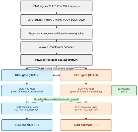
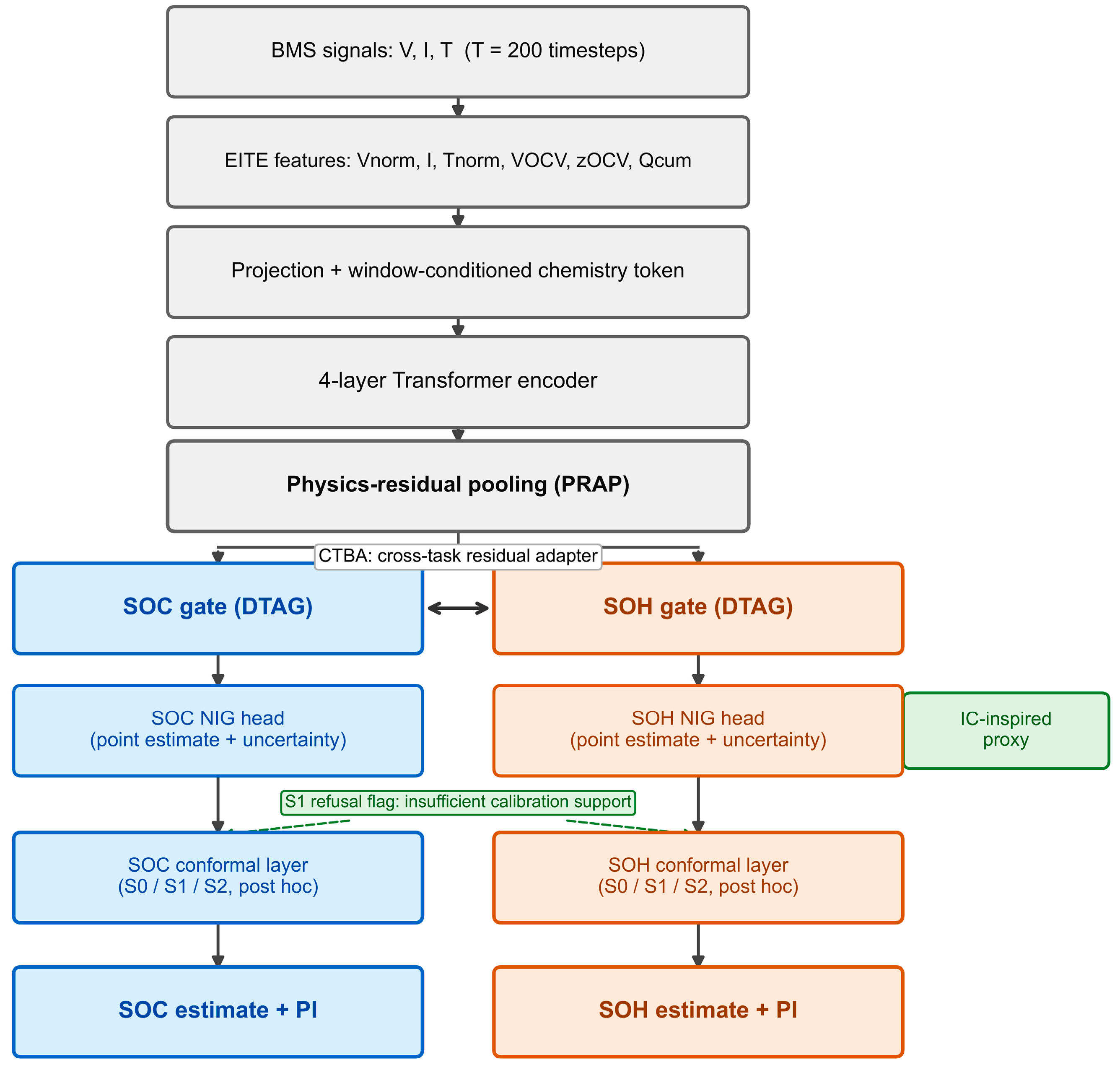
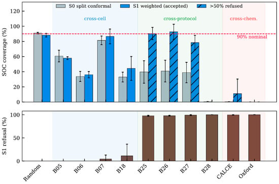
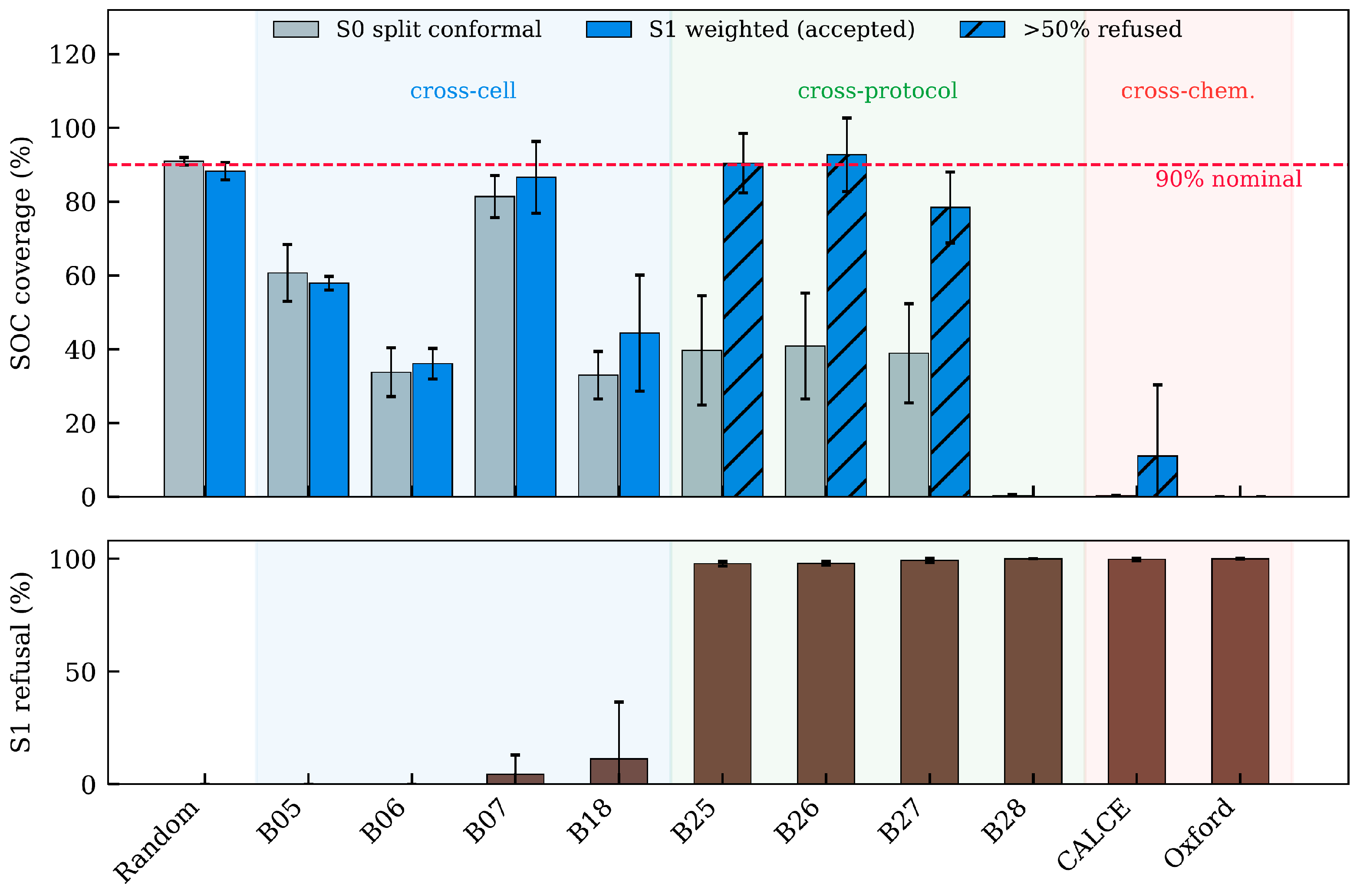
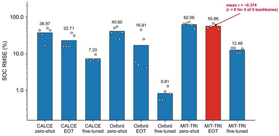
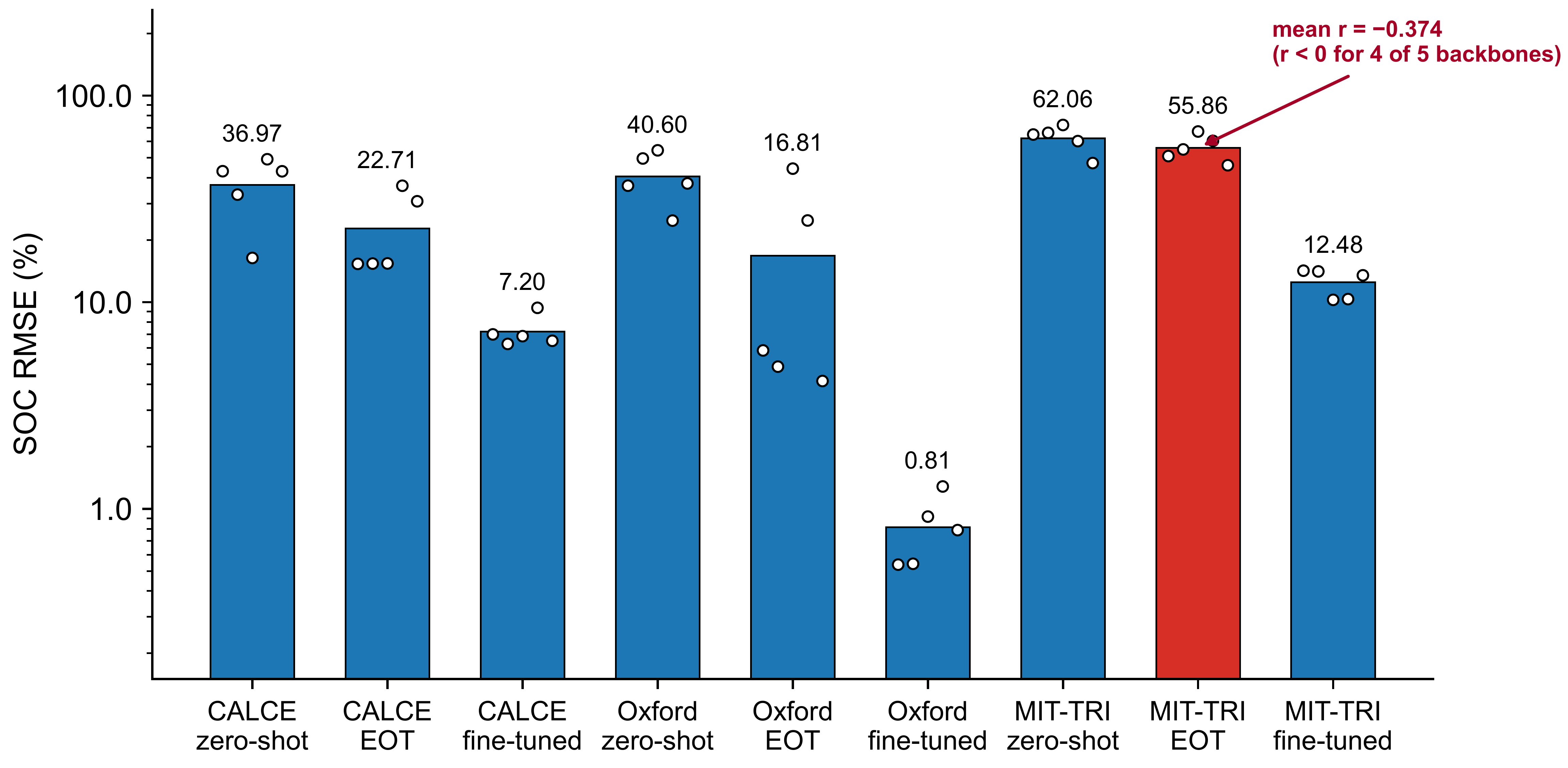

Disclaimer/Publisher’s Note: The statements, opinions and data contained in all publications are solely those of the individual author(s) and contributor(s) and not of MDPI and/or the editor(s). MDPI and/or the editor(s) disclaim responsibility for any injury to people or property resulting from any ideas, methods, instructions or products referred to in the content. |
© 2026 by the authors. Licensee MDPI, Basel, Switzerland. This article is an open access article distributed under the terms and conditions of the Creative Commons Attribution (CC BY) license.