Collaborative Optimization Scheduling Method for Distribution Networks and Microgrids Based on Analytical Target Cascading

Abstract

The growing penetration of distributed generation has led to an increasing number of microgrids being integrated into distribution networks, which introduces considerable difficulties in reconciling the divergent economic interests of multiple stakeholders while maintaining information privacy. To address these issues, this study proposes a collaborative optimization dispatching model for distribution network–microgrid systems based on Analytical Target Cascading (ATC). A bi-level optimization framework is established, consisting of an upper-level active–reactive power coordination model for the Active Distribution Network (ADN) and a lower-level joint dispatch model for multiple microgrids incorporating load-side demand response. The ATC algorithm is employed to decompose the centralized optimization problem into independent subproblems, enabling iterative coordination between levels while preserving stakeholder privacy. Four scenarios are designed and simulated on an IEEE 33-node system for comparative analysis. The results demonstrate that the proposed method significantly reduces total system operating costs and improves voltage profiles compared with independent ADN operation. The ATC-based distributed solution achieves a cost deviation of only 0.46% from the centralized optimum, while safeguarding proprietary information of all participants. The approach exhibits good convergence and numerical stability, confirming its engineering applicability in multi-stakeholder collaborative scheduling.

1. Introduction

With the continuous increase in distributed generation penetration, the integration of numerous microgrids into distribution networks has become a key trend in modern power system development. As controllable units, microgrids can integrate distributed energy sources, energy storage systems, and loads, thereby enhancing power supply reliability while facilitating renewable energy integration. However, the integration of microgrids also poses new challenges for distribution network operation and dispatch: distribution networks and microgrids operate under distinct stakeholder interests, each prioritizing optimal operational efficiency; traditional centralized optimization and dispatch methods struggle to balance these conflicting objectives and face issues such as information privacy concerns and excessive computational demands. Against this backdrop, how to achieve collaborative optimization dispatch between distribution networks and microgrids while safeguarding the interests of all stakeholders has become a critical technical bottleneck in the development of new power systems [1,2].

In the field of ADN optimization dispatch, extensive research has been conducted by scholars worldwide. A day-ahead and intra-day collaborative dispatch method for ADNs based on optimal economic operation regions was proposed, which improves system economic efficiency and renewable energy accommodation capability by coordinating multi-timescale resources [3]. To address the difficulties in model maintenance and strong randomness caused by large-scale integration of distributed resources, a machine learning-based energy management and operation control technical framework for ADNs was developed, effectively reducing dependence on accurate model parameters [4]. A multiple correlation model that simultaneously considers spatio-temporal correlation and conditional correlation was constructed to address the impact of renewable energy variability on dispatch decisions in ADNs, and an active–reactive power coordinated optimization dispatch framework was established based on this model [5]. Through stochastic model predictive control, it achieves coordinated management of fast and slow response resources, effectively suppressing node voltage fluctuations and reducing system operating costs. In [6], for the coordinated dispatch of multiple types of resources in ADNs, a day-ahead and intra-day two-timescale optimization dispatch model covering energy storage, flexible loads, and controllable distributed generation was established. With the dual objectives of minimizing system operating costs and maximizing renewable energy accommodation, a hybrid optimization method combining differential evolution and imperialist competitive algorithms is employed, achieving synergistic improvements in operating cost reduction and renewable energy accommodation enhancement.

In the field of distribution network–microgrid collaborative optimization, a stochastic optimization dispatch model for multi-microgrid economic operation was constructed through probabilistic modeling of source–load outputs for multi-microgrid systems containing various small-scale distributed energy resources, and was solved using particle swarm optimization, verifying that power interaction between microgrids and the main grid can effectively reduce total system operating costs [7]. Microgrids were integrated as bidirectional dispatchable units into distribution networks [8], where the maximum input and output power margins of microgrids were evaluated through multi-timescale unbalanced energy prediction, and an economic optimization active power dispatch model was established with these margins as interaction power constraint boundaries, achieving effective reduction in system operating costs and network losses. In [9], a strategy for multiple microgrids to lease shared energy storage and form a microgrid coalition was proposed to address the issues of low energy storage utilization efficiency and insufficient renewable energy accommodation in multi-microgrid grid-connected systems. A leader-multiple-follower Stackelberg game model is constructed with the distribution network as the leader and the microgrid coalition and shared energy storage operator as followers, achieving coordinated improvement in stakeholder interest balance and local renewable energy accommodation through time-of-use tariff incentives and two-stage optimization dispatch. Heterogeneous prosumers were aggregated into virtual microgrids through communication systems [10], and a Stackelberg game model was constructed with producers as leaders and consumers as followers, achieving coordinated optimization of energy procurement costs, producer utility, and carbon emissions through equilibrium pricing and distributed optimization.

However, while the aforementioned studies have made important progress in constructing distribution network–microgrid collaborative dispatch models, the centralized or game-theoretic optimization methods employed all require stakeholders to share complete internal information, facing issues of privacy leakage and excessive communication burdens [11]. Moreover, the practical implementation of these distributed dispatch models is fundamentally constrained by the underlying communication infrastructure. In harsh smart grid environments, wireless sensor networks (WSNs) are subjected to severe electromagnetic interference and dynamic spectrum scarcity, which necessitates advanced spectrum-aware and capacity-aware communication frameworks to ensure reliable data transmission [12]. At the distribution level, the neighborhood area networks (NANs) serve as the critical link between substations and end-users; however, the heterogeneous communication standards and protocol stacks in NANs pose substantial challenges in achieving low-latency and reliable last-mile connectivity [13]. Furthermore, a comprehensive review of smart grid communication highlights the inherent trade-offs in selecting communication mediums and switching technologies, which directly affect the availability, security, and efficiency of control signals [14]. Specifically, in networked microgrids, the choice of communication architecture—whether master-slave, publish-subscribe, or event-triggered—profoundly influences the operational autonomy, privacy preservation, and fault tolerance of the energy management system [15]. Consequently, the proposed hierarchical coordination framework must align with these communication constraints to ensure practical engineering feasibility. ADNs and microgrids typically belong to different stakeholders, and how to achieve hierarchical collaborative optimization between ADNs and microgrids while protecting the privacy of each stakeholder has become an important research topic. In [16], an energy management model for ADNs and microgrids was constructed, and the Alternating Direction Method of Multipliers (ADMM) was employed to achieve coordinated optimization, improving system economic efficiency and renewable energy accommodation while protecting the data privacy of each operator. In [17], a distributed online collaborative dispatch algorithm for networked microgrid clusters was proposed, coordinating the real-time dispatch decisions of each microgrid through an online ADMM framework, providing a distributed implementation approach for the collaborative optimization dispatch of ADNs and microgrid clusters. The ATC method was employed to coordinate energy interaction between distribution companies and multiple microgrids, solving for the optimal operating points of each independent system through hierarchical optimization iterations, laying a theoretical foundation for the application of ATC in distribution network–microgrid collaborative optimization [18]. An optimization dispatch model and solution method based on ATC theory was proposed for the decentralized autonomous characteristics of active distribution systems containing multiple microgrids [19]. With production efficiency optimization as the objective, chance constraints are employed to describe uncertainties such as distributed generation output and load forecasting errors, treating microgrids and distribution networks as different stakeholders. The coupling between distribution network and microgrid operations is decoupled by equivalently representing tie-line power as virtual generators and virtual loads, enabling parallel solution of the microgrid autonomous model and the distribution network optimization model. In [20], a non-hierarchical ATC framework without the need for a central coordinator was proposed, decomposing the ADN dispatch problem containing multiple interconnected microgrids into several local dispatch models for parallel solution. By introducing auxiliary variables to constrain the types of coupling variables between subsystems, it significantly reduces computational complexity while protecting the information privacy and operational autonomy of microgrids.

However, as a widely adopted distributed optimization method, ADMM has inherent limitations when dealing with the non-convex or multi-block distributed models commonly encountered in hierarchical power systems, where its direct extension does not guarantee convergence. To address this issue, a Prediction-Correction-based ADMM (PCB-ADMM) has been developed to enhance numerical stability [21]. Nevertheless, PCB-ADMM remains fundamentally a dual-decomposition approach oriented towards homogeneous peer-to-peer architectures, requiring complex Lagrangian multiplier handling. In contrast, the ATC method adopted in this study is built upon a hierarchical decomposition architecture that naturally aligns with the leader-follower physical structure of the ADN and multiple MGs. Through bidirectional iterative coordination of target values and response values, ATC offers clearer physical semantics, stronger robustness, and lower communication overhead, thereby effectively safeguarding the decision-making autonomy and information privacy of all stakeholders.

Distribution networks and microgrids constitute hierarchical heterogeneous systems, where significant differences exist between upper and lower levels in terms of decision variable types and objective structures. Most existing distributed approaches are designed for peer-to-peer homogeneous subsystems, making them difficult to apply directly. As an effective distributed optimization framework, the ATC method enables the progressive decomposition of upper-level objectives into sub-objectives for lower-level subsystems, facilitates iterative exchange of boundary variable information between levels, and ultimately achieves coordinated resolution of the global optimum.

Based on the aforementioned approach, this study establishes a bi-level distributed collaborative optimization scheduling model for the distribution network–microgrid system based on ATC. First, it describes the network topology of the distribution network, the allocation of distributed resources, and the operational characteristics of various voltage regulation and reactive power equipment; second, it develops separate optimization models for the upper-level distribution network and the lower-level microgrid, specifying the objective functions, decision variables, and operational constraints for each level; third, it establishes a hierarchical iterative solution model based on ATC to perform distributed solving for the bi-level system; finally, case simulations are conducted to verify the effectiveness of the proposed model and algorithm.

2. Distribution Network–Microgrid Operational Architecture

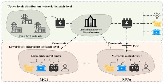
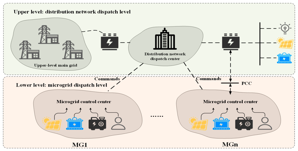
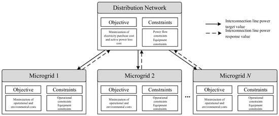
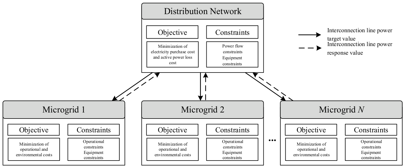
The bi-level dispatch architecture for distribution networks and microgrids is illustrated in Figure 1. The collaborative operational architecture of distribution networks and microgrids typically exhibits a multi-level, distributed hybrid topology that combines master-slave and peer-to-peer configurations, with its core objective being the deep integration of wide-area source-grid-load-storage and global energy optimization. Within this architecture, the distribution network serves as the upper-level coordination center, leveraging advanced monitoring systems and wide-area communication technologies to centrally manage power flow distribution, node voltages, and energy trading across the regional grid while enforcing boundary constraints; the microgrid functions as a lower-level active node with high autonomy, organically integrating distributed generation sources, energy storage systems, and flexible loads into a unified whole.

Figure 1. Distribution network–microgrid operational architecture.

3. Bi-Level Optimization Model for Distribution Network–Microgrid Systems

3.1. Bi-Level Optimization Theory

Bi-level optimization is a hierarchical optimization problem comprising two levels: upper-level optimization and lower-level optimization. The upper-level problem is typically referred to as the leader problem, while the lower-level problem is termed the follower problem; together, they form a hierarchical decision-making relationship [22]. The core feature of this theory is that the constraints in the upper-level optimization problem implicitly contain the optimal solution for the lower-level problem. This implies that the decision-making processes at both levels are mutually constraining and deeply coupled: the upper level must anticipate the optimal response of the lower level when formulating its strategy, whereas the decision space of the lower level is directly constrained by the parameters of the upper-level strategy.

In the collaborative optimization scenario between distribution networks and microgrids, the general form of the bi-level optimization model can be expressed as:

Optimization problem of the upper-level distribution network:

$${\min }_{x_u}{F}_u(x_u,x_l^{*})$$

(1)

$$s.t.G_u(x_u,x_l^{*})\le 0$$

(2)

$$H_u(x_u,x_l^{*})=0$$

(3)

Optimization problem of the lower-level microgrid:

$${\min }_{x_l}{F}_l(x_u,x_l)$$

(4)

$$s.t.G_l(x_u,x_l)\le 0$$

(5)

$$H_l(x_u,x_l)=0$$

(6)

where $F_u(x_u,x_l^{*})$ represents the objective function of the upper-level distribution network, reflecting the interests of the upper-level leader; $F_l(x_u,x_l)$ represents the objective function of the lower-level microgrid, reflecting the interests of the follower; $x_u$ denotes the decision variable of the upper-level distribution network; $x_l$ denotes the decision variable of the lower-level microgrid; and $x_l^{*}$ represents the optimal response of each microgrid under a given dispatch signal.

In the collaborative optimization dispatching model between distribution networks and microgrids, the distribution network serves as the upper-level leader, possessing comprehensive network information. Its primary tasks include formulating macro-level electricity procurement and sales plans, reactive power compensation schemes, and power allocation strategies for interconnection lines to achieve optimal overall system benefits. Each microgrid acts as a lower-level follower: upon receiving boundary information from the distribution network, it optimizes its distributed generation output, energy storage charging/discharging operations, and flexible load response strategies while maintaining internal supply-demand balance, then feeds back the final response data to the upper level. Physical power exchange via interconnection lines and data interaction between the upper and lower levels are carried out through iterative processes, ultimately achieving a globally coordinated equilibrium state.

3.2. Active–Reactive Power Optimization Dispatch Model for Upper-Level Active Distribution Networks

As the critical hub connecting the upper-level main grid with lower-level microgrids, the dispatch decisions of the distribution network directly impact the economic efficiency and security of the entire system. To fully leverage the optimization potential at the distribution network level and achieve coordinated utilization of active and reactive power resources, a scientifically sound upper-level optimization dispatch model must be developed. This study establishes the upper-level distribution network model as an ADN with the objectives of minimizing both grid connection costs to the main grid and distribution network active power loss costs. Under constraints imposed by power flow equations, node voltage safety requirements, branch current capacity limits, and operational boundaries of all equipment, the model performs joint optimization of active and reactive power resources, thereby constructing a coordinated active–reactive power optimization dispatch model for the upper-level ADN.

3.2.1. Objective Function

As the top-level decision-maker, ADN aims to minimize economic costs while ensuring safe operation. In this study, ADN’s economic costs consist of two components: electricity procurement costs from the main grid and active power loss costs in the distribution network, expressed as follows:

$$C_{ADN}={\displaystyle \sum _{\mathrm{t}=1}^T(c_{buy,up}{P}_{up}(t)+c_{loss}{P}_{loss}(t))}$$

(7)

where $c_{buy,up}$ represents the price of electricity purchased by ADN from the main grid during the period t; $P_{up}(t)$ represents the power of electricity purchased by ADN from the main grid during the period t; $c_{loss}$ represents the unit cost coefficient for ADN active power loss; and $P_{loss}(t)$ represents the active power loss of ADN during the period t.

3.2.2. Constraints

• Power Flow Constraints

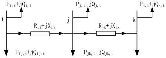
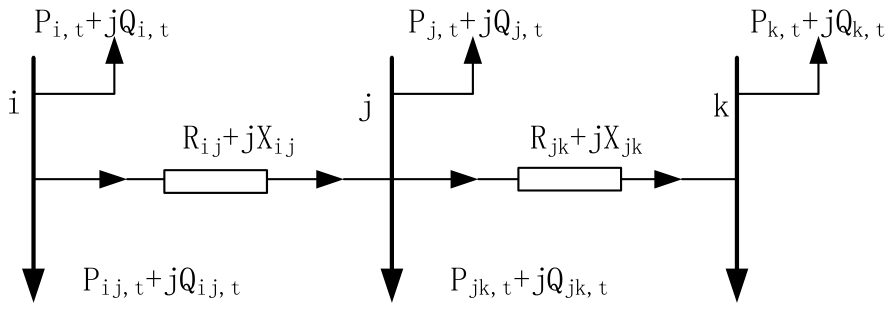
Distribution networks typically adopt a radial topology with a high impedance ratio, and traditional node-admittance-matrix-based power-flow calculation methods often encounter convergence issues in such networks. Therefore, this section employs the Branch Flow Model (DistFlow) to describe the steady-state operating characteristics of distribution networks and introduces Second-Order Cone Programming (SOCP) [23] relaxation techniques to transform power flow constraints into a second-order cone model. The schematic diagram of a radial distribution network is shown in Figure 2.

Figure 2. Schematic diagram of a radial distribution network structure.

The constraints that the power flow in this branch must satisfy are:

$$U_{j,t}^2=U_{i,t}^2-2(R_{ij}{P}_{ij,t}+X_{ij}{Q}_{ij,t})+(R_{ij}^2+X_{ij}^2)I_{ij,t}^2$$

(8)

$$P_{i,t}=P_{ij,t}-R_{ij}{I}_{ij,t}^2-{\displaystyle \sum _{k.j\to k}{P}_{ik,t}}$$

(9)

$$Q_{i,t}=Q_{ij,t}-X_{ij}{I}_{ij,t}^2-{\displaystyle \sum _{k.j\to k}{Q}_{jk,t}}$$

(10)

$$I_{ij,t}^2={\displaystyle \frac{P_{ij}^2+Q_{ij}^2}{U_{i,t}^2}}$$

(11)

Due to the non-convex nature of the quadratic power flow equation constraints in the aforementioned model, solving it is typically challenging; therefore, second-order cone relaxation [24] is employed to transform it into a more solvable optimization problem. Introducing Equation (12) converts the quadratic terms into linear terms:

$${\tilde{U}}_{i,t}=U_{i,t}^2,{\tilde{I}}_{i,t}=I_{i,t}^2$$

(12)

The power flow constraints for the distribution network are expressed in the following second-order cone form:

$$‖\begin{array}{c}2P_{ij,t}\\ 2Q_{ij,t}\\ {\tilde{I}}_{ij,t}-{\tilde{U}}_{ij,t}\end{array}‖\le {\tilde{I}}_{ij,t}+{\tilde{U}}_{ij,t}$$

(13)

2.

Photovoltaic Output Constraints

Solar resources constrain photovoltaic power generation, and its actual output must not exceed the predicted maximum available power.

$$0\le P_{PV,j}^{ADN}(t)\le P_{PV,\max }^{ADN}(t),j\in {\Omega }_{PV}$$

(14)

$${(P_{PV,j}^{ADN}(t))}^2+{(Q_{PV,j}^{ADN}(t))}^2\le {(S_{PV,\max }^{ADN})}^2$$

(15)

$$-P_{PV,j}^{ADN}(t)\tan {\theta }_{PV}\le Q_{PV,j}^{ADN}(t)\le P_{PV,j}^{ADN}(t)\tan {\theta }_{PV}$$

(16)

where $P_{PV,\max }^{ADN}(t)$ represents the predicted maximum available photovoltaic power during the period t, $S_{PV,\max }^{ADN}$ denotes the maximum apparent power of photovoltaic output; $P_{PV,j}^{ADN}(t)$ denotes the active power generated by the photovoltaic units connected to node j of the distribution network at time t; and $Q_{PV,j}^{ADN}(t)$ denotes the reactive power generated by the photovoltaic units connected to node j of the distribution network at time t.

3.

Energy Storage Constraints

Charging and discharging Power Constraints:

$$0\le P_{ch,j}^{ADN}(t)\le P_{ESS,\max }^{ADN}{u}_{ch}(t),j\in {\Omega }_{ESS}$$

(17)

$$0\le P_{dis,j}^{ADN}(t)\le P_{ESS,\max }^{ADN}{u}_{dis}(t),j\in {\Omega }_{ESS}$$

(18)

where $P_{ESS,\max }^{ADN}$ represents the maximum charging and discharging power of energy storage connected to the distribution network; $u_{ch}(t)$ and $u_{dis}(t)$ are binary variables (0 or 1) indicating the charging and discharging states, respectively, satisfying $u_{ch}(t)+u_{dis}(t)\le 1$, which means that simultaneous charging and discharging are not permitted during the same time period; $P_{ch,j}^{ADN}(t)$ and $P_{dis,j}^{ADN}(t)$ represent the charging and discharging power of the energy storage at node j of the distribution network during the period t.

State of Charge constraints:

$$SO{C}_j(t)=SO{C}_j(t-1)+\left({\eta }_{ch}{P}_{ch,j}^{ADN}(t)-{\displaystyle \frac{P_{dis,j}^{ADN}(t)}{{\eta }_{dis}}}\right){\displaystyle \frac{\mathsf{\Delta }t}{E_{ESS}}},j\in {\Omega }_{ESS}$$

(19)

$$SO{C}_{\min }\le SO{C}_j(t)\le SO{C}_{\max }, j\in {\Omega }_{ESS}$$

(20)

where $SOC(t)$ represents the state of charge at the end of period t; ${\eta }_{ch}$ and ${\eta }_{dis}$ denote the charging and discharging efficiency of the energy storage system respectively; $E_{ESS}$ is the rated capacity of the energy storage system; and $SO{C}_{\min }$ and $SO{C}_{\max }$ represent the upper and lower limits of the state of charge.

4.

Parallel Capacitor Bank

Shunt capacitor banks (CB) represent the most fundamental and widely used reactive power compensation devices. Their primary function is to inject reactive power into the grid, thereby enhancing voltage levels at end nodes and reducing active power losses in interconnection lines. Unlike continuously adjustable reactive power sources, traditional capacitor banks typically consist of multiple capacitor units with identical capacities connected in parallel, switched via mechanical switches. The operational constraints for shunt capacitor banks are as follows:

$$Q_j^{CB}(t)=N_j^{CB}(t)\mathsf{\Delta }{Q}_j^{CB}, j\in {\Omega }_{CB}$$

(21)

$$N_j^{CB}(t)\le N_{j,\max }^{CB}, j\in {\Omega }_{CB}$$

(22)

$$u_j^{CB}(t)\le \left|\left.N_j^{CB}(t)-N_j^{CB}(t-1)\right|\le N_{j,\max }^{CB}{u}_j^{CB}(t), j\in {\Omega }_{CB}\right.$$

(23)

$${\displaystyle \sum _{t=1}^T{u}_j^{CB}}(t)\le U_{\max }^{CB}, j\in {\Omega }_{CB}$$

(24)

where $Q_j^{CB}(t)$ represents the reactive power output of the CB at node j during the time t; $\mathsf{\Delta }{Q}_j^{CB}$ represents the reactive capacity of a single capacitor bank; $N_j^{CB}(t)$ represents the number of active capacitor banks; $N_{j,\max }^{CB}$ represents the maximum number of active capacitor banks; $u_j^{CB}(t)$ is a binary variable where 1 indicates a change in the number of active banks and 0 indicates no change; $U_{\max }^{CB}$ represents the maximum number of switching operations for CB within the dispatch cycle; and ${\Omega }_{CB}$ represents the set of nodes to which CB is connected in the distribution network.

5.

Static Var Compensator

The Static Var Compensator (SVC) is a dynamic reactive power compensation device based on power electronics technology, capable of achieving rapid and continuous regulation of reactive power. It serves as a critical component for improving distribution network voltage quality and enhancing system stability.

Unlike the discrete regulation of CB, SVC offers millisecond-level response speed and continuous adjustability, enabling rapid tracking of fluctuating system reactive power demands while suppressing voltage fluctuations and flicker—making it ideal for variable loads and renewable energy integration scenarios. The SVC’s reactive power output can be expressed as:

$$Q_{SCV,\min }\le Q_{SCV}(t)\le Q_{SCV,\max }$$

(25)

where $Q_{SCV,\max }$ and $Q_{SCV,\min }$ represent the upper and lower limits of SVC’s reactive power output, respectively.

3.3. Optimization Dispatch Model for Lower-Level Microgrids

The objective function for the lower-level microgrid comprises two components: operational costs and pollutant treatment costs, expressed as follows:

$$\min C_{MG}=C_{OM}+C_F+C_{grid}+C_{IBDR}+C_{EN}$$

(26)

where $C_{OM}$ represents the microgrid operation and maintenance cost; $C_F$ represents the microgrid fuel cost; $C_{grid}$ represents the interaction cost between the microgrid and the distribution network; $C_{IBDR}$ represents the incentive-based demand response compensation cost; and $C_{EN}$ represents the pollutant treatment cost.

The operational cost for the lower-level microgrid includes microgrid operation and maintenance costs, microgrid fuel costs, interaction costs between the microgrid and the distribution network, and incentive-based demand response compensation costs; however, within this distribution network–microgrid system, when the microgrid purchases electricity from the upstream distribution network, although pollutants are not emitted locally, pollutant emissions also occur at the generation side of the main grid. Therefore, this paper includes the treatment costs associated with these pollutant emissions within the microgrid’s overall pollution control expenses. The expression for the microgrid’s pollution treatment cost is as follows:

$$C_{EN}={\displaystyle \sum _{t=1}^T{\displaystyle \sum _{k=1}^K(c_{k,DE}{q}_{k,DE}{P}_{DE,t}(t)+c_{k,ADN}{q}_{k,ADN}{P}_{ADN,t}(t))}}$$

(27)

where $c_{k,DE}$ and $c_{k,ADN}$ represent the cost coefficients for treating the k-th pollutant on the diesel generator side and the large power grid generation side, respectively; and $q_{k,DE}$ and $q_{k,ADN}$ represent the emissions of the k-th pollutant generated by the diesel generator side and the large power grid generation side during operation, respectively.

The modeling approach and constraint conditions for the lower-level microgrid model mainly include power balance constraints, unit output constraints, energy storage operation constraints, demand response constraints, and interaction constraints with the distribution network.

• Power Balance Constraints

In the operation of the microgrid, the total power supply and the load-side demand must maintain power balance, as shown in Equation (28):

$$P_{PV}\left(t\right)+P_{ESS}\left(t\right)+P_{DE}\left(t\right)+P_{buy}\left(t\right)=P_{load}\left(t\right)+P_{sell}\left(t\right)$$

(28)

where $P_{load}\left(t\right)$ denotes the total load of the microgrid after demand response during period t.

2.

Photovoltaic Output Constraints

Photovoltaic generation is limited by solar resources, and its actual output must not exceed the predicted maximum available power:

$$0\le P_{ch}(t)\le P_{PV,\max }(t)$$

(29)

where $P_{PV,\max }(t)$ denotes the predicted maximum available photovoltaic power during period t.

3.

Energy Storage System Constraints

Charging and Discharging Power Constraints:

$$0\le P_{ch}(t)\le P_{ESS,\max }{u}_{ch}(t)$$

(30)

$$0\le P_{dis}(t)\le P_{ESS,\max }{u}_{dis}(t)$$

(31)

where $P_{ESS,\max }$ denotes the maximum charging and discharging power of the energy storage system, and $u_{ch}(t)$ and $u_{dis}(t)$ are binary variables (0 or 1) indicating the charging and discharging states, respectively, satisfying $u_{ch}(t)+u_{dis}(t)\le 1$, meaning that simultaneous charging and discharging are not permitted during the same time period.

State of Charge Constraints:

$$SOC(t)=SOC(t-1)+\left({\eta }_{ch}{P}_{ch}(t)-{\displaystyle \frac{P_{dis}(t)}{{\eta }_{dis}}}\right){\displaystyle \frac{\mathsf{\Delta }t}{E_{ESS}}}$$

(32)

$$SO{C}_{\min }\le SOC(t)\le SO{C}_{\max }$$

(33)

where $SOC(t)$ denotes the state of charge at the end of period t; ${\eta }_{ch}$ and ${\eta }_{dis}$ denote the charging and discharging efficiencies of the energy storage system, respectively; $E_{ESS}$ is the rated capacity of the energy storage system; and $SO{C}_{\max }$ and $SO{C}_{\min }$ represent the upper and lower limits of the state of charge, respectively.

4.

Diesel Generator Constraints

Upper and Lower Output Limits:

$$P_{DE,\min }\le P_{DE}(t)\le P_{DE,\max }(t)$$

(34)

where $P_{DE,\max }$ and $P_{DE,\min }$ are the upper and lower output limits of the diesel generator, respectively.

Ramp Rate Constraints:

$$-R_{DE,\min }\le P_{DE}(t)-P_{DE}(t-1)\le R_{DE,\max }$$

(35)

where $R_{DE,\max }$ and $R_{DE,\min }$ are the maximum upward and downward ramp rates of the diesel generator, respectively.

5.

Interaction Constraints with the Distribution Network

The exchange power between the microgrid and the distribution network is limited by the transmission capacity of the interconnection line and must not exceed the maximum allowable value:

$$0\le P_{buy}(t)\le P_{grid,\max }, 0\le P_{sell}(t)\le P_{grid,\max }$$

(36)

where $P_{grid,\max }$ is the maximum transmission power of the interconnection line.

6.

Incentive-Based Demand Response Constraints

Curtailable Load Constraints:

$$-P_{cut,\max }\le P_{cut}(t)\le 0$$

(37)

where $P_{cut,\max }$ denotes the maximum available capacity of curtailable loads during period t.

Shiftable Load Constraints:

$$-P_{shift,\max }\le P_{shift}(t)\le P_{shift,\max }(t)$$

(38)

$${\displaystyle \sum _{t=1}^T{P}_{shft}(t)}\mathsf{\Delta }t=0$$

(39)

where $P_{shift,\max }(t)$ denotes the maximum shiftable power of shiftable loads during period t; Equation (39) ensures that the total electricity consumption remains unchanged before and after load shifting, i.e., the amount of load shifted out and shifted in must be balanced.

4. Bi-Level Optimization Solution Strategy for Distribution Networks and Microgrids

4.1. Theoretical Basis of Analytical Target Cascading

The ATC method is a distributed coordinated optimization framework specifically designed for hierarchical nested systems, first proposed by scholars Kim and Michelena et al. [25], and subsequently widely applied in hierarchical decision-making scenarios such as power system dispatching, supply chain management, and transportation network design. Its core concept involves decomposing a tightly coupled large-scale optimization problem into multiple subproblems with hierarchical relationships based on the system’s physical or managerial structure. Each subsystem operates autonomously locally while achieving global consistency through iterative coordination of shared coupling variables, ultimately approximating the global optimal solution without centralized information aggregation. The ATC method offers significant advantages—including a clear hierarchical structure, well-defined physical semantics, and the capability to solve subsystems fully in parallel—making it particularly suitable for bi-level optimization scenarios where upper and lower decision-makers are relatively independent yet deeply interconnected through common variables despite differing objectives.

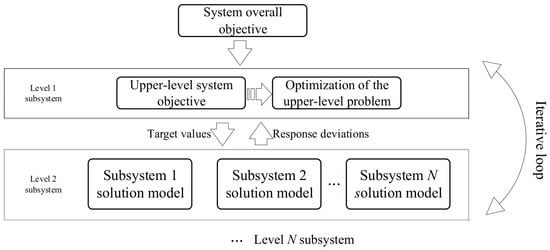
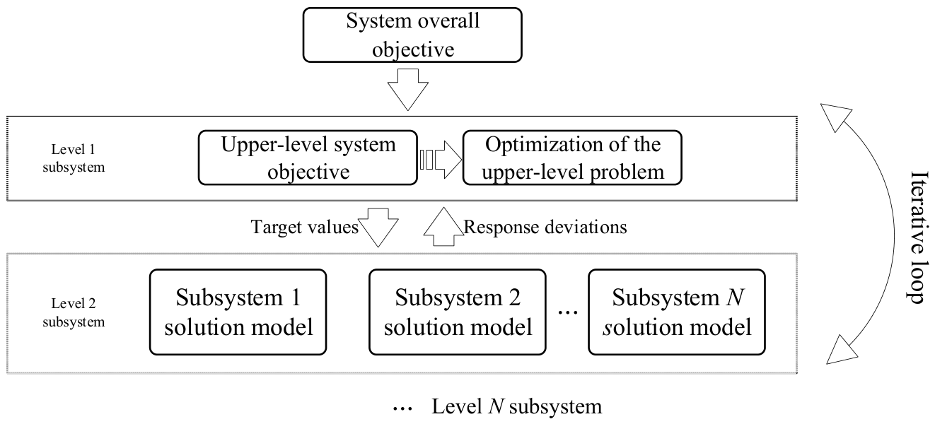
The ATC objective decomposition structure is illustrated in Figure 3. This model exhibits a typical hierarchical tree-like decomposition topology, with the system’s top level encompassing the overall design objectives. Global problems are progressively broken down level by level, each containing multiple independent nodes that represent distinct mathematical programming models responsible for solving their respective local decision spaces. Regarding inter-level information exchange, adjacent levels maintain a bidirectional variable transmission mechanism: upper levels pass design objective variables (i.e., target values expected from lower levels), while lower levels return response deviations (i.e., discrepancies between actual solution values and target values). This bidirectional interaction persists throughout the iterative solution process, enabling subsystems at each level to gradually eliminate inconsistencies through repeated negotiation to reconcile design objectives and response deviations while maintaining local autonomy. Ultimately, this approach achieves coordinated alignment between global system objectives and localized optimization goals under constraints, enabling efficient distributed resolution of the original large-scale coupled optimization problem.

Figure 3. ATC objective decomposition structure diagram.

4.2. ATC-Based Distributed Solving Method

The distribution network and microgrid studied in this paper operate in parallel through dedicated interconnection lines, forming a typical “leader–following” bi-level coupling structure. Under this architecture, the distribution network assumes coordinated dispatch responsibilities for both global safety and economic efficiency, while microgrids connect to the distribution network via PCCs through interconnection lines, maintaining autonomous energy management and engaging in real-time power exchange with the distribution network. The objectives of the two levels are relatively distinct: the upper-level distribution network prioritizes minimizing electricity procurement costs from the main grid and active power loss costs; the lower-level microgrids aim to minimize their respective overall economic costs. Their deep interdependence is driven by the critical coupling variable of interconnection line power, meaning dispatch decisions at either level directly impact the operational status of the other, constituting a classic bi-level coupling optimization problem.

For the aforementioned bi-level coupling optimization problem, adopting a centralized solution approach requires the distribution network dispatch center to possess comprehensive knowledge of each microgrid’s internal topology parameters, equipment constraints, and user load data. This not only poses significant risks of information privacy breaches but also leads to exponential growth in computational complexity as the number of microgrids increases, making solution efficiency difficult to guarantee. To address this, this section employs ATC as a distributed solution framework for the bi-level optimization problem, decomposing the large-scale centralized optimization task into upper-level distribution network subproblems and lower-level microgrid subproblems. Through iterative negotiation between target power values and response values at interconnection nodes, an efficient global collaborative optimal solution can be achieved while ensuring the information privacy and decision-making autonomy of all stakeholders.

Based on the hierarchical decomposition principle of the ATC method, the bi-level optimization problem for distribution networks and microgrids is mapped to a bi-level ATC tree structure: the first level represents the upper-level distribution network optimization subproblem, while the second level corresponds to the lower-level microgrid optimization subproblem. Information exchange between levels is facilitated through the power of interconnection lines as the core coupling variable. The detailed decomposition framework is illustrated in Figure 4.

Figure 4. Bi-level decomposition framework for distribution network–microgrid ATC.

Within the ATC decomposition framework, the upper-level distribution network subproblem and the lower-level microgrid subproblems are bidirectionally coupled through the target values and response values of interconnection line power. Information exchange between the two levels is mediated by ${\tilde{P}}_{PCC,i}^{ADN}$ and ${\tilde{P}}_{PCC,i}^{MG}$ that represent both the transmitted target interconnection line power from the distribution network side and the returned response value from the microgrid side; these quantities converge to equality at the optimal solution, thereby achieving coordinated decoupling across hierarchical levels.

Based on the original operating cost objective $C_{ADN}$, the upper-level distribution network subproblem incorporates a penalty function term addressing the power inconsistency of all N lines, thereby constructing the following augmented objective function:

$$\min C_{ADN}+{\displaystyle \sum _{n=1}^N\pi (P_{PCC,n}^{ADN}-{\tilde{P}}_{PCC,n}^{MG})}$$

(40)

$$s.t.g_{ADN}\le 0,h_{ADN}=0$$

(41)

where $C_{ADN}$ is the objective function representing the operational cost of the distribution network itself; $P_{PCC,i}^{ADN}$ represents the decision value for power allocation on the n-th interconnection line by the upper-level distribution network; ${\tilde{P}}_{PCC,i}^{MG}$ denotes the power response value of the n-th interconnection line transmitted back from the microgrid in the previous iteration; and $g_{ADN}\le 0$ and $h_{ADN}=0$ include both inequality constraints and equality constraints applicable to the distribution network. $\pi (·)$ is the ATC penalty function operator, defined as follows:

$$\pi (P_{PCC,i}^{ADN}-{\tilde{P}}_{PCC,i}^{MG})={\displaystyle \sum _{t=1}^T\left[{\lambda }_n^k(P_{PCC,n}^{ADN,t}-{\tilde{P}}_{PCC,n}^{MG,t})+{\omega }_n^k{(P_{PCC,n}^{ADN,t}-{\tilde{P}}_{PCC,n}^{MG,t})}^2\right]}$$

(42)

where ${\lambda }_n^k$ is the Lagrange multiplier for the n-th interconnection line at the k-th iteration; ${\omega }_n^k$ is the corresponding quadratic penalty weight.

The solution result $P_{PCC,n}^{ADN,k+1}$ of the upper-level subproblem is transmitted to each microgrid as the new round of target value ${\tilde{P}}_{PCC,n}^{ADN}$. Upon receiving the interconnection line power target ${\tilde{P}}_{PCC,i}^{ADN}$ from the upper level, the n-th microgrid constructs the following augmented objective function:

$$\min C_{MG,n}+\pi (P_{PCC,n}^{MG}-{\tilde{P}}_{PCC,n}^{ADN})$$

(43)

$$s.t.g_{MG,n}\le 0,h_{MG,n}=0$$

(44)

where $C_{MG,n}$ represents the operational cost objective function of the n-th microgrid; $P_{PCC,n}^{MG}$ denotes the power response variable of the interconnection line to be optimized on the microgrid side; ${\tilde{P}}_{PCC,n}^{ADN}$ is the power response value of the interconnection line returned from the distribution network in the previous iteration; and $g_{MG,n}\le 0$ and $h_{MG,n}=0$ include both inequality constraints and equality constraints applicable to the microgrid. The penalty term $\pi (·)$ ensures that the actual power response of the microgrid’s interconnection lines tracks the target values specified by the upper-level system, with an expression similar to that in Equation (45).

$$\pi (P_{PCC,n}^{MG}-{\tilde{P}}_{PCC,n}^{ADN})={\displaystyle \sum _{t=1}^T\left[{\lambda }_n^k(P_{PCC,n}^{MG,t}-{\tilde{P}}_{PCC,n}^{ADN,t})+{\omega }_n^k{(P_{PCC,n}^{MG,t}-{\tilde{P}}_{PCC,n}^{ADN,t})}^2\right]}$$

(45)

Once all subproblems of the microgrid have been solved, the response value $P_{PCC,n}^{MG,k+1}$ is transmitted back to the upper-level coordination level as ${\tilde{P}}_{PCC,n}^{MG}$.

After all subproblems at both upper and lower levels are solved in each iteration, the coordination level updates the Lagrange multiplier based on the residual difference between the target power value of the interconnection line and its actual response value.

$${\lambda }_n^{k+1}={\lambda }_n^k+2{({\omega }_n^k)}^2(P_{PCC,n}^{ADN,k+1}-P_{PCC,n}^{MG,k+1})$$

(46)

And update the penalty weights according to the adaptive strategy:

$${\omega }_n^{k+1}=\left\{\begin{array}{c}\beta {\omega }_n^k,{\displaystyle {\displaystyle \sum _{t=1}^T}\left|\left.P_{PCC,n}^{ADN,k+1}-P_{PCC,n}^{MG,k+1}\right|\right.}>\gamma {\displaystyle {\displaystyle \sum _{t=1}^T}\left|\left.P_{PCC,n}^{ADN,k}-P_{PCC,n}^{MG,k}\right|\right.}\\ {\omega }_n^k, otherwise\end{array}\right.$$

(47)

The iteration is terminated, and the optimal scheduling scheme is output only when the power consistency residual ${\epsilon }^k$ of all interconnection lines simultaneously satisfies the convergence criterion given below:

$${\epsilon }^k=\max \left|\left.P_{PCC,n}^{ADN,k}-P_{PCC,n}^{MG,k}\right|\right.\le {\epsilon }_{\min }$$

(48)

where ${\epsilon }_{\min }$ is the convergence threshold.

In summary, the ATC bi-level optimization scheduling model decomposes the originally large-scale coupled optimization problem—which required centralized N solving—into one upper-level distribution network subproblem and several completely independent lower-level microgrid subproblems through iterative negotiations of interconnection line power value ${\tilde{P}}_{ACC,n}^{ADN}$ and ${\tilde{P}}_{ACC,n}^{MG}$. Under the strict protection of operational privacy for all stakeholders, a multiplier-driven distributed iteration mechanism ultimately achieves globally coordinated optimality.

4.3. Model Solving Process

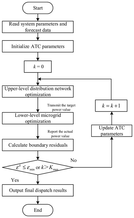
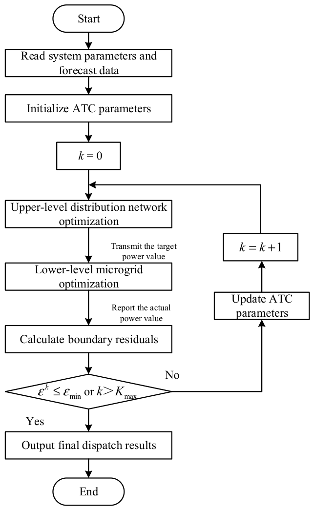
The construction process of the aforementioned model demonstrates that there is a strong coupling relationship between the distribution network subproblem and the microgrid subproblem, mediated by power coupling variables on interconnection lines. The proposed ATC distributed solution framework uses interconnection line power exchange as a coordination mechanism to decompose the original coupled problem into two independent subproblems at different levels. Each level independently solves its own optimization task solely based on the target values and response values of interconnection line power, while the coordination level continuously reduces inter-level power inconsistency residuals through rolling updates of augmented Lagrange multipliers, driving the system toward a globally coordinated optimal solution. The complete solution process is illustrated in Figure 5, with each step described as follows:

Figure 5. Solution process for ADN–microgrid collaborative optimization scheduling based on ATC.

Step 1: Initialize system parameters and iteration variables. Read fundamental data including the network topology of the distribution grid and each microgrid, equipment operating boundaries, photovoltaic output prediction sequences, and load prediction sequences; set initial values of power coupling variables for all interconnection lines to zero, $P_{PCC,n}^0=0$; set initial values of Lagrange multipliers to zero, ${\lambda }_n^0=0$; define initial penalty weight, ${\omega }_n^0={\omega }_0$; and assign a current iteration number, $k=1$.

Step 2: Optimization solution at the distribution network level. The upper-level distribution network dispatch center uses the current multiplier ${\lambda }_n^{k-1}$, penalty weight ${\omega }_n^{k-1}$, and the power response value $P_{PCC,n}^{MG,k-1}$ of the interconnection lines transmitted from the previous microgrid round as known parameters to solve the augmented subproblem for the distribution network described in Equation (40): while minimizing both the electricity purchase cost from the main grid and the active power loss cost of the distribution network, it constrains the decision value $P_{PCC,n}^{ADN,k}$ of the distribution-side interconnection lines to converge toward the microgrid response value via the penalty function term; after solving the distribution network subproblem, the updated interconnection line power target value ${\tilde{P}}_{PCC,n}^{ADN,k}$ is transmitted to each microgrid via communication channels as the coordination boundary conditions for the respective microgrid subproblems in this round.

Step 3: Parallel optimization solution at the microgrid level. Upon receiving the target power value ${\tilde{P}}_{PCC,n}^{ADN,k}$ for the interconnection lines from the distribution network, each microgrid independently solves the augmented subproblem of the microgrid described in Equation (43): minimizing operational and pollutant treatment costs while driving the response values of the microgrid-side interconnection lines toward the distribution network’s target value $P_{PCC,n}^{MG,k}$. There is no direct coupling between the subproblems, allowing them to be executed entirely in parallel to enhance computational efficiency; after solving, each microgrid reports the corresponding interconnection line power response value ${\tilde{P}}_{PCC,n}^{MG,k}$ to the distribution network coordination level.

Step 4: Convergence Test and Iteration Control. If the residual ${\epsilon }_k$ has converged within the preset tolerance ${\epsilon }_{\min }$ and the relative change in the system’s overall objective function meets the convergence accuracy requirements, the current solution is deemed to have achieved optimal coordination; the iteration is terminated, and the optimal dispatch schemes for both the distribution network and each microgrid are output respectively. If the convergence conditions are not yet satisfied, the Lagrange multiplier ${\lambda }_n^k$ and penalty weight ${\omega }_n^k$ for each link are updated according to Equations (46) and (47), the iteration counter is reset to $k+1$, and the process returns to Step 2 to initiate the next iteration. The power coupling variables between the distribution network and each microgrid are continuously updated through the aforementioned closed-loop iteration mechanism of “target generation → parallel response → multiplier correction” until the inter-level power mismatch residual falls within the tolerance range, ultimately yielding an optimal operating scheme that satisfies the global coordination consistency constraint.

5. Case Study Analysis

5.1. Example Settings

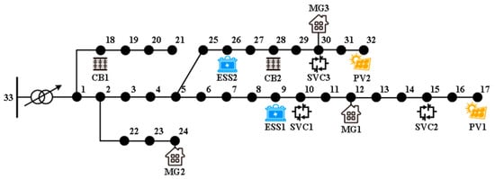
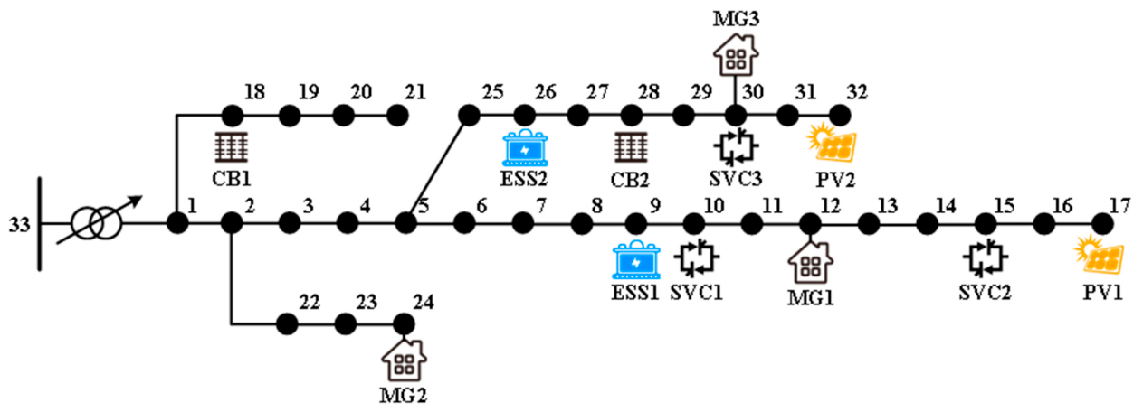
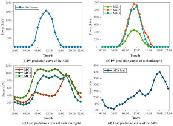
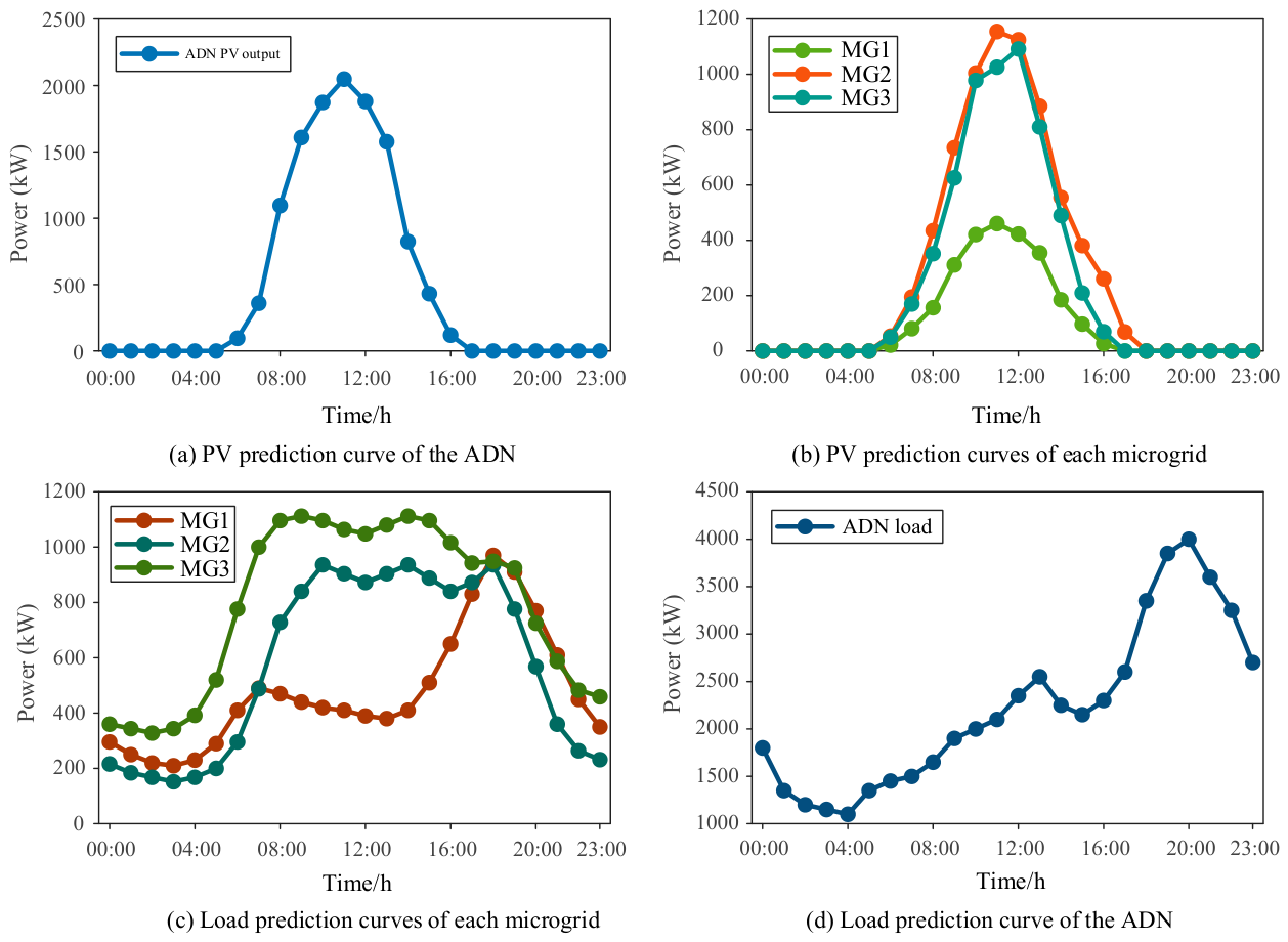
To validate the effectiveness of the ATC-based distribution network–microgrid optimization scheduling method proposed in this study, a 33-node IEEE system was selected for simulation verification, with its topology shown in Figure 6. Node 33 is connected to upper-level nodes; Nodes 12, 24, and 30 are linked to MG1, MG2, and MG3 respectively; Nodes 17 and 32 are connected to photovoltaic (PV) systems; Nodes 9 and 26 are connected to energy storage systems (ESS); Nodes 10, 15, and 30 are connected to Static Var Compensators (SVC) with a reactive power regulation range of −100 kvar to 300 kvar. Nodes 18 and 28 are connected to shunt capacitor banks (CB), with a maximum of 5 banks in operation (each rated at 100 kvar) and a maximum switching operation count of 5. The operation and maintenance costs are set at 0.001 RMB/kWh for PV systems, 0.02 RMB/kWh for energy storage systems, and 0.128 RMB/kWh for diesel generators; configurations for diesel generators and energy storage systems are detailed in Table 1 and Table 2. Power limits for interconnections between MGs and the ADN are specified in Table 3; The electricity purchase and sale tariffs between MG and the ADN are as follows: during peak hours, the purchase price is 0.65 RMB/kWh and the sale price is 0.50 RMB/kWh; during off-peak hours, the purchase price is 0.38 RMB/kWh and the sale price is 0.28 RMB/kWh; during valley hours, the purchase price is 0.23 RMB/kWh and the sale price is 0.10 RMB/kWh. The ADN’s electricity purchase price from the main grid is set at 0.90 RMB/kWh during peak hours, 0.65 RMB/kWh during off-peak hours, and 0.35 RMB/kWh during valley hours; pollutant emission fees are listed in Table 4. Load and PV generation forecasts are presented in Figure 7.

Figure 6. Topological diagram of the distribution network–microgrid system.

Table 1. Diesel generator parameters.

Type	Power Upper Limit (kW)	Lower Power Limit (kW)	Maximum Ramping Power (kW/h)
DG-MG1	700	0	150
DG-MG2	700	0	150
DG-MG3	600	0	150

Table 2. Energy storage configuration.

Type	Rated Capacity (kWh)	Initial SOC	SOC Upper Limit	SOC Lower Limit	Maximum Charge/Discharge Power (kW)	Charge/Discharge Efficiency
ESS1-ADN	1200	0.50	0.95	0.15	300	0.9
ESS2-ADN	1500	0.50	0.90	0.20	300	0.9
ESS-MG1	600	0.40	0.95	0.20	250	0.95
ESS-MG2	700	0.50	0.90	0.15	200	0.95
ESS-MG3	700	0.40	0.95	0.20	250	0.95

Table 3. Interconnection line constraints.

Interconnection Line	ADN-MG1	ADN-MG2	ADN-MG3
Power Limit (kW)	500	700	700

Table 4. Costs of pollutant emissions.

Pollutant Type	Processing Cost (RMB/kg)	Pollutant Emission Factor (g/kWh)
		Diesel Generator	ADN
CO2	0.21	720	875
SO2	6	0.004	1.80
NOx	8	0.617	1.60

Figure 7. Load and photovoltaic prediction curves.

5.2. Result Analysis

To verify how the coordinated optimization scheduling of distribution networks and microgrids enhances ADN operational performance and overall economic efficiency, four scenarios were designed for comparative analysis:

Scenario 1: The ADN is not connected to the MG and is optimized independently.

Scenario 2: The ADN connects to the MG, where load-side demand response is implemented; however, only the MG reports the interconnection line power. The ADN uses this as a known input for optimization, with no feedback coordination between them.

Scenario 3: The ADN is connected to the MG with a collaborative optimization framework adopted, but does not account for load-side demand response within the MG; the MG relies solely on distributed power sources and energy storage for regulation.

Scenario 4: The ADN is connected to the MG with a collaborative optimization framework adopted, and load-side demand response is implemented within the MG, fully leveraging the regulatory potential of flexible loads.

The system operating costs under the four scenarios are shown in Table 5. Although Scenario 2 incorporates Microgrids and demand response mechanisms, the absence of feedback coordination between the ADN and MGs prevents MGs from perceiving electricity procurement cost pressures on the ADN side during independent optimization. This leads MGs to reduce their generation output while heavily relying on ADN power purchases, resulting in higher electricity procurement costs and network loss expenses for the ADN compared to Scenario 1 without MG integration, with total system costs significantly exceeding those of Scenarios 3 and 4. These findings demonstrate that without coordinated feedback mechanisms, even implemented demand response measures at MG sites are offset by cost shifts caused by information asymmetry, ultimately increasing operational burdens on the ADN. By adopting a centralized collaborative optimization framework integrating distribution networks and microgrids in Scenario 3, both electricity procurement costs and network losses for the ADN decrease markedly compared to Scenario 2, reducing total system costs to ¥57,914.62. Under this collaborative framework, MGs are incentivized to fully leverage their regulatory potential as distributed energy sources and storage units, effectively curbing disorderly power purchase demands from the ADN and significantly improving its operational efficiency. Scenario 4 further introduces load-side demand response within MGs, reducing MG fuel costs and pollutant emission costs by 16.9% and 10.2%, respectively, compared to Scenario 3, transforming MGs from passive load nodes into active units with transmission capabilities. Total system costs drop to RMB 52,138.67—a 9.97% reduction from Scenario 3—robustly demonstrating how load-side demand response enhances overall system economics within a collaborative optimization framework.

Table 5. Comparison of costs for each scenario.

Economic Cost (RMB)	Scenario 1	Scenario 2	Scenario 3	Scenario 4
Network Loss Cost	846.26	1272.69	713.36	618.79
ADN Electricity Purchase Cost from the Main Grid	26,735.64	41,537.89	28,685.27	27,046.85
MG Operation and Maintenance Cost	-	924.62	3884.10	3648.29
MG Fuel Cost	-	2593.19	19,056.82	15,816.38
MG Electricity Purchase Cost from ADN	-	8372.10	184.10	−721.94
MG Pollutant Emission Cost	-	5207.57	5390.98	4843.61
MG-IBDR Compensation Cost	-	512.62	0.00	886.70
Total Cost	-	60,420.67	57,914.62	52,138.67

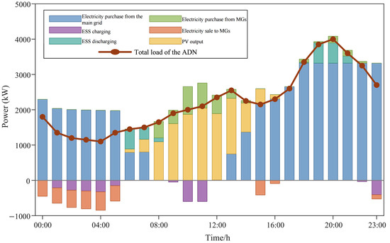
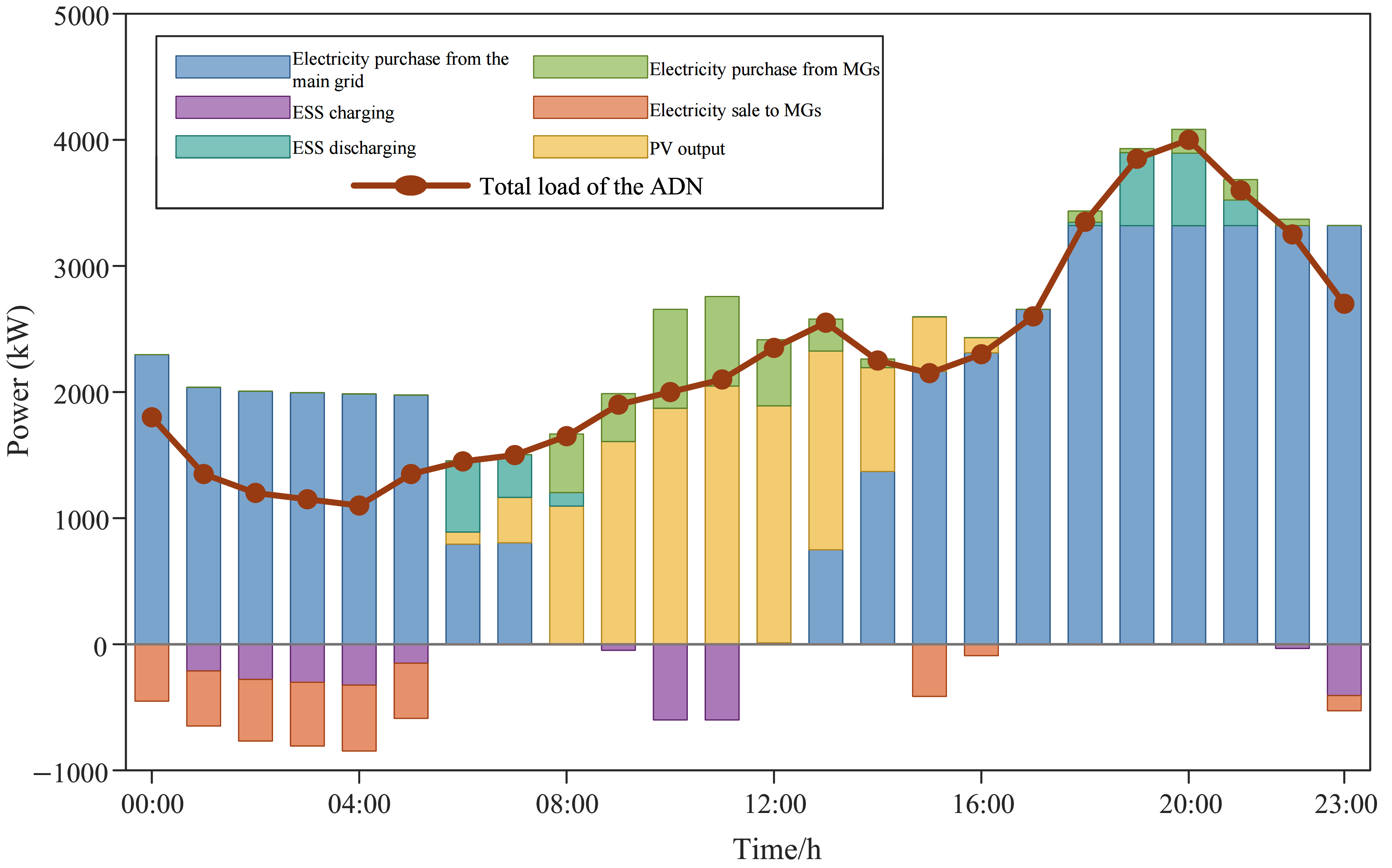
Figure 8 illustrates the power balance diagram of the ADN under Scenario 4. Overall, the ADN’s power supply primarily relies on electricity procurement from the main grid, supplemented by coordinated output from PV systems, Energy Storage Systems (ESS), and microgrids during various time periods. After 08:00, photovoltaic generation begins increasing steadily and peaks between 12:00 and 16:00, significantly reducing the ADN’s electricity purchases from the main grid during this period. The ESS charges during daytime hours when PV output is high and during early morning periods when electricity prices are lower, while discharging during evening peak demand times to mitigate load fluctuations. The ADN’s electricity purchases from microgrids mainly occur during daytime periods with strong PV output, demonstrating that microgrids can supply power to the ADN when their distributed resources are abundant, providing essential support. Conversely, electricity sales from the ADN to microgrids concentrate during early morning hours when prices are lower and demand is low. Overall, Scenario 4 achieves comprehensive power balance and cost-effective operation through the coordinated timing of ESS charging and discharging, the local utilization of PV generation, and the bidirectional power interaction between the ADN and the microgrids.

Figure 8. Power balance diagram of ADN under Scenario 4.

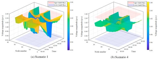
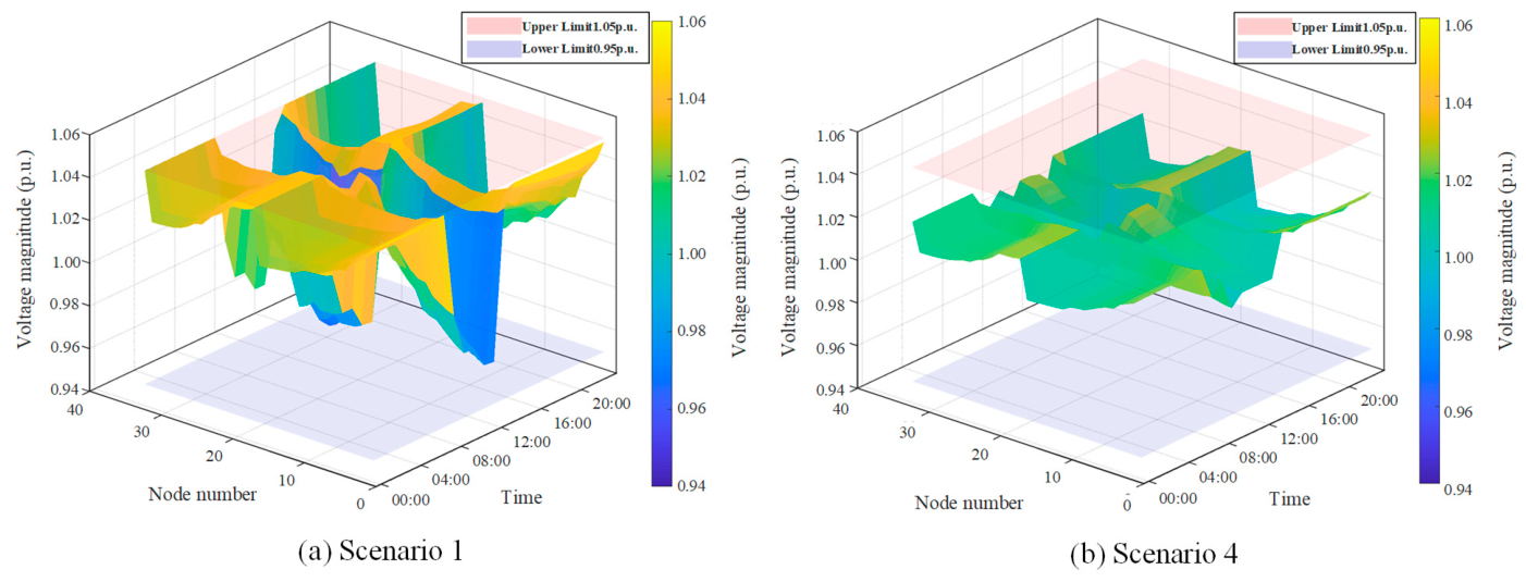
The three-dimensional voltage distribution surfaces of ADN nodes under Scenario 1 and Scenario 4 are shown in Figure 9. The figures reveal that both scenarios exhibit a general decline in voltage levels during peak load periods. In Scenario 1, due to the absence of microgrid integration, the ADN relies solely on grid power supply and its own distributed resources to maintain power balance, lacking active regulation support from flexible loads within the microgrid; consequently, voltage drops at end nodes during peak hours are more pronounced, with significant fluctuations in the voltage profile. In contrast, Scenario 4 incorporates a microgrid and load-side demand response mechanisms, enabling flexible loads within the microgrid to actively reduce power consumption during peak hours, thereby providing effective active power support to the ADN. This results in a more stable overall voltage profile across the network, significantly improved voltage valley mitigation at end nodes, and greater voltage margin relative to the baseline level. These findings demonstrate that the combined operation of ADN-MG collaborative optimization and load-side demand response not only enhances system economics but also substantially improves voltage distribution quality and increases voltage safety margins during operation.

Figure 9. Three-dimensional voltage distribution surfaces of ADN nodes.

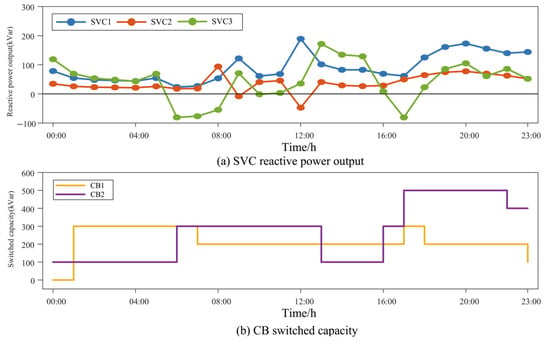
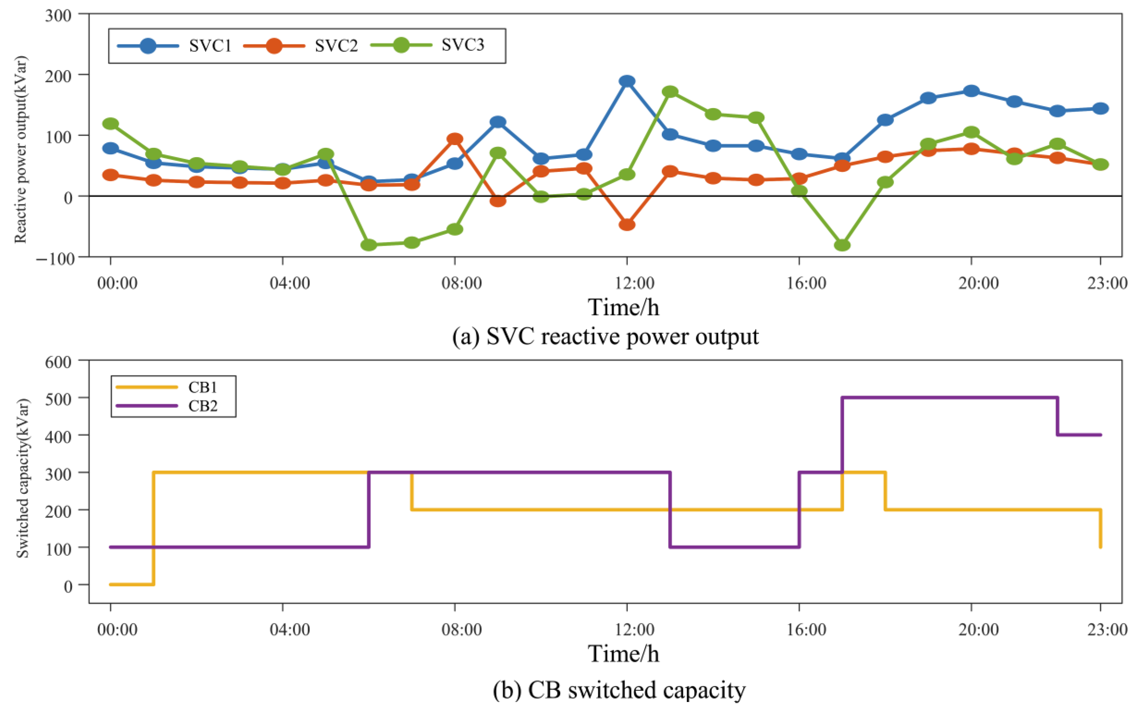
Figure 10 illustrates the daily output profiles of the ADN reactive power regulation devices, SVC and CB, under Scenario 4. As shown in Figure 10a, the daily outputs of all three SVC units closely align with system load fluctuations. SVC1 consistently maintained inductive reactive power output throughout the day, reaching peak levels during evening peak hours to provide sustained voltage support at the terminal node, demonstrating the most stable regulatory performance. SVC2 exhibited brief reactive power absorption episodes during morning hours, indicating that localized photovoltaic generation caused elevated node voltages; SVC2 promptly switched to capacitive operation to prevent voltage exceedance. SVC3 displayed more pronounced absorption activities, maintaining significant reactive power absorption during early morning peak periods, reflecting greater sensitivity to photovoltaic generation impacts and stronger voltage surge pressures in this region. Subsequently, as photovoltaic output stabilized and loads continued to rise, all three SVC units returned to inductive operation modes and worked collaboratively to maintain voltage stability during evening peak hours under high-power power flow conditions, demonstrating the continuous reactive power regulation system’s rapid response capability to voltage fluctuations. Figure 10b reveals distinct operational differentiation between the two CB units in terms of switching behavior. CB1 primarily operates at a moderate capacity, initially engaging during off-peak hours to meet basic reactive power demands and gradually reducing its contribution during peak hours, demonstrating a relatively conservative overall regulation approach; CB2, in contrast, plays a more proactive role in supporting reactive power demand during peak periods, surging significantly during the morning rush hour, briefly withdrawing during midday, then operating at full capacity throughout the evening peak period and maintaining this level for an extended duration until a slight decline occurs late at night, effectively responding to sustained high loads during nighttime. Both CB units provide fundamental capacity support for system reactive power compensation through coarse-grained switching operations, complementing the continuous regulation capabilities of SVCs and enhancing the overall economic efficiency and equipment utilization rate of reactive power management.

Figure 10. Daily output performance of the ADN reactive power regulation devices, SVC and CB, under Scenario 4.

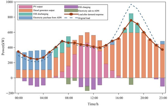
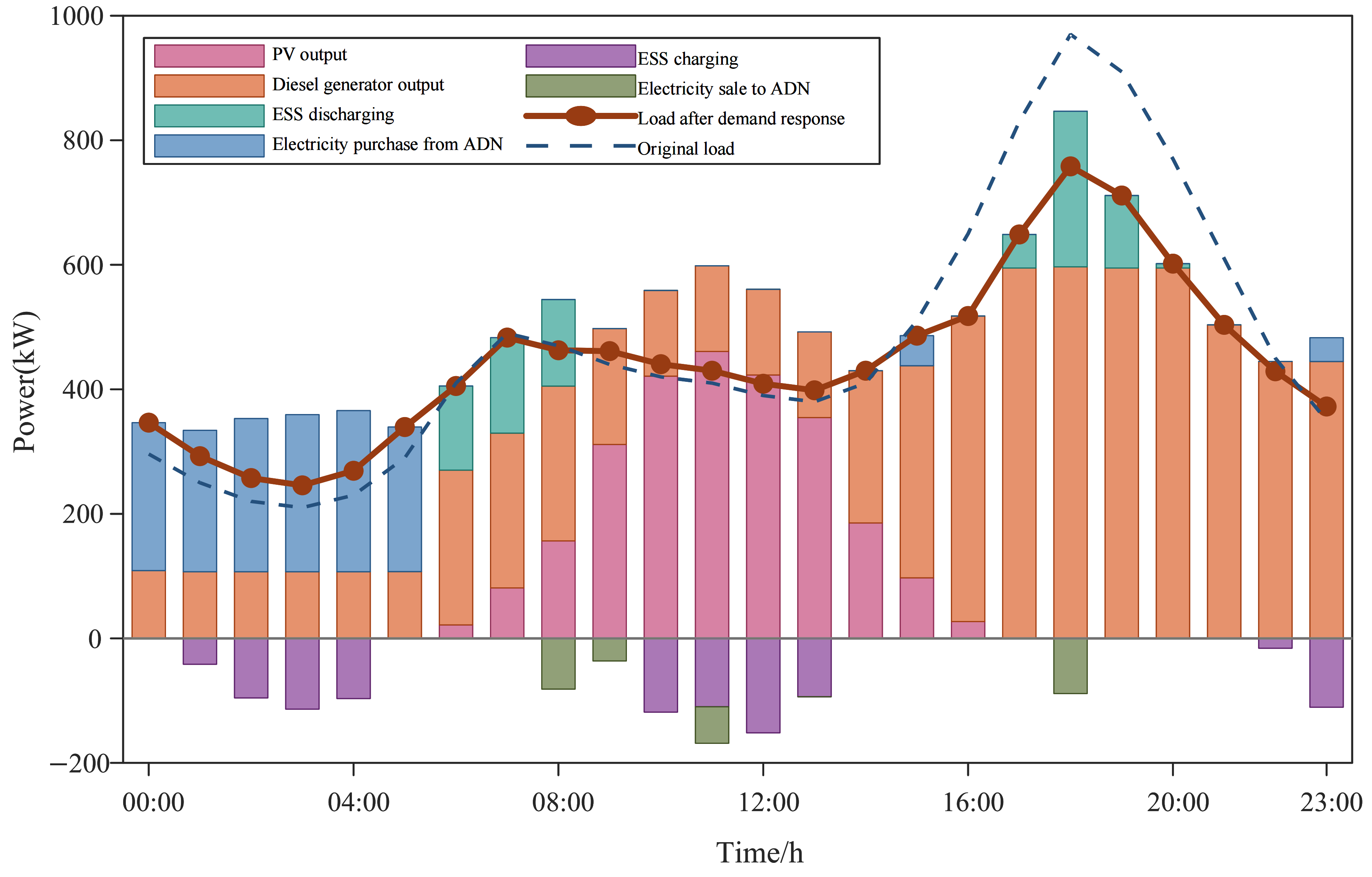
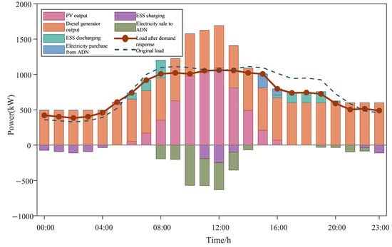
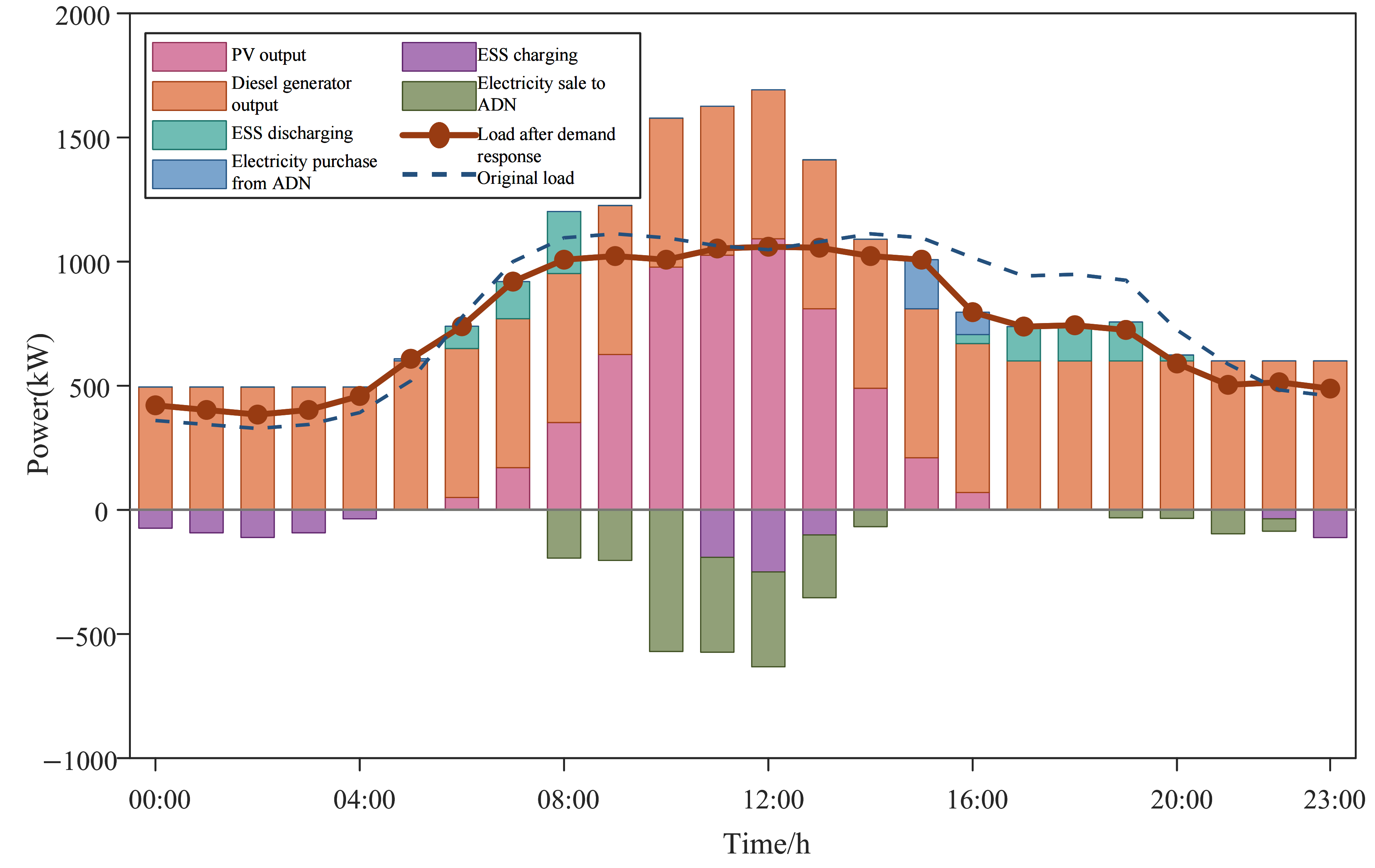
Figure 11, Figure 12 and Figure 13 illustrate the full-day power dispatch plans for three microgrids under Scenario 4. As shown in Figure 11, MG1’s supply side primarily relies on diesel generators, which operate continuously throughout the day with stable output, serving as the main load supplier. Photovoltaic systems exhibit significant peak generation during daytime; when combined with diesel power, their combined output exceeds local demand, enabling MG1 to sell electricity to the ADN at the highest price—with surplus power being fed back to the ADN, demonstrating the synergistic benefits of localized consumption and surplus transmission from distributed resources. Energy storage systems perform time-shaving functions by charging during nighttime off-peak hours and discharging during peak demand periods, effectively mitigating power fluctuations. Demand response measures prove highly effective in MG1, significantly reducing flexible loads during evening peaks and flattening the load curve, thereby expanding MG1’s power surplus for daytime electricity sales to the ADN and achieving bidirectional optimization between load and supply sides.

Figure 11. MG1’s daily power dispatch schedule.

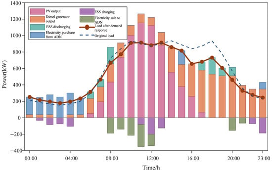
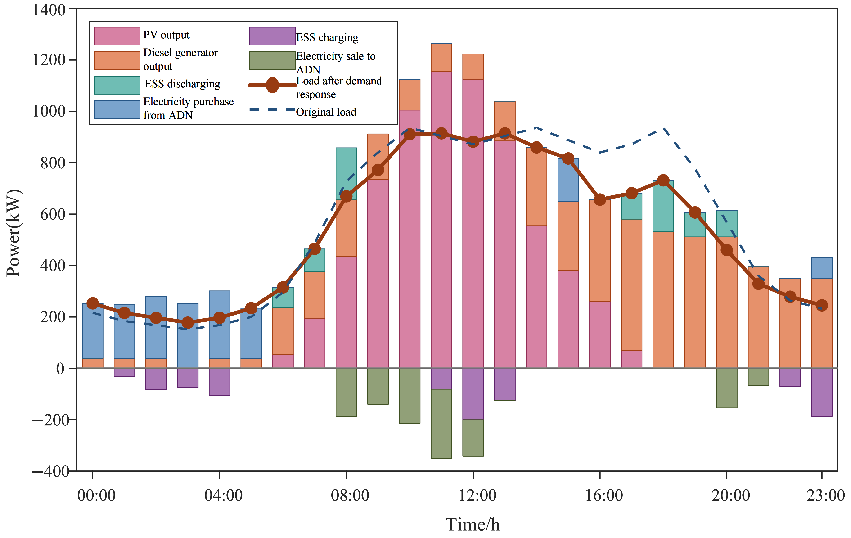
Figure 12. MG2’s daily power dispatch schedule.

Figure 13. MG3’s daily power dispatch schedule.

As shown in Figure 12, MG2’s photovoltaic power generation plays a dominant role. After photovoltaic output ceases at night, MG2 relies entirely on electricity purchased from ADN to meet its load demand, with this purchasing need persisting throughout the night. During daytime hours, as photovoltaic output rises rapidly, MG2 gradually reduces its dependence on ADN and transitions into net electricity exporting mode during peak generation periods. Energy storage systems charge extensively during periods of high photovoltaic output to absorb surplus electricity; when output declines sharply in the evening, they promptly switch to discharge mode, working in tandem with diesel generators to support nighttime load demand. This approach effectively mitigates the pronounced intermittent fluctuations in photovoltaic output and reduces power exchange variations between MG2 and ADN.

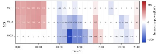
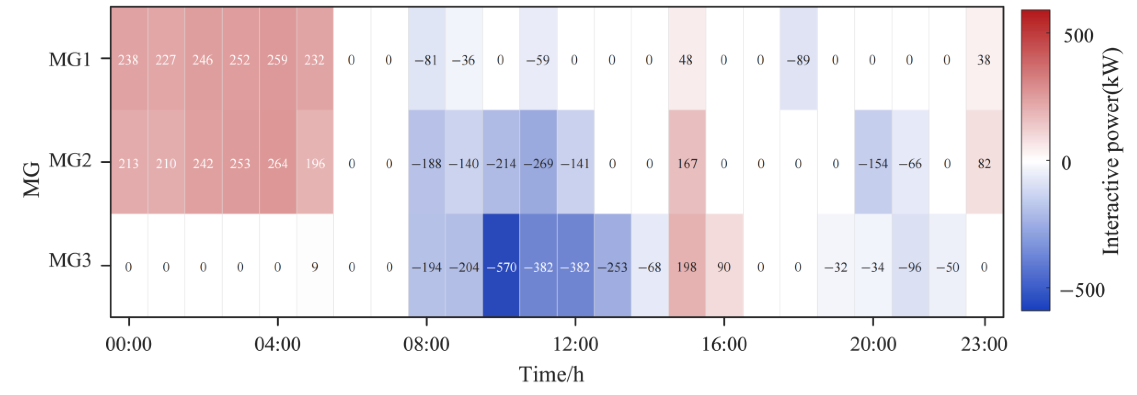
As shown in Figure 13, the most distinctive feature of MG3 is its power interaction with the ADN, exhibiting a pronounced unidirectional electricity purchasing dominance. Figure 14 presents the heat map of power interactions between each microgrid and the ADN interconnection lines; positive values indicate electricity purchases from the ADN, while negative values represent electricity sales to the ADN. The figure reveals that during daytime peak solar generation periods, MG3’s electricity sales volume to the ADN is the highest among the three microgrids, characterized by prolonged duration and substantial power magnitude. Conversely, MG3 hardly purchases electricity from the ADN throughout the day; even after solar generation ceases at night, the combined output from the diesel generator and energy storage system sufficiently meets its own load demands, eliminating reliance on the ADN for power supplementation.

Figure 14. Power heat map of the interconnection lines.

Overall, each microgrid is capable of feeding power back to the ADN during daytime periods of abundant solar generation, while at night it relies to varying degrees on ADN electricity purchases or diesel generator output to maintain balance, forming a natural time-sharing complementary support framework. The implementation of demand response has played a positive role in peak shaving and valley filling across all microgrids, resulting in smoother load curves post-response, thereby enhancing local utilization efficiency of distributed resources and reducing overall power fluctuations on the ADN for the entire microgrid cluster.

The total system operating costs for Scenario 4 obtained using the ATC distributed algorithm and those from the centralized optimization are shown in Table 6. As indicated in the table, the difference between the ATC-based distributed solution and the centralized approach is merely 0.46% in total system cost; the operating costs of ADN and individual microgrids closely match the centralized results, demonstrating that ATC can still generate a scheduling scheme close to the global optimum under this two-tier architecture, with solution accuracy meeting application requirements.

Table 6. Comparison between centralized and distributed solving methods.

Economic Cost (RMB)	Centralized	ATC-Based Distributed
ADN	27,665.64	27,710.54
MG1	8295.84	8383.85
MG2	6788.32	6936.11
MG3	9388.87	9347.25
Total Cost	52,138.67	52,377.75

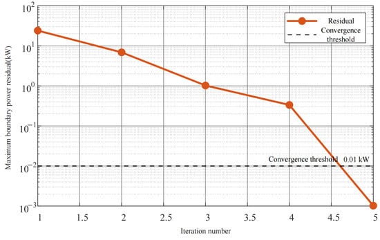
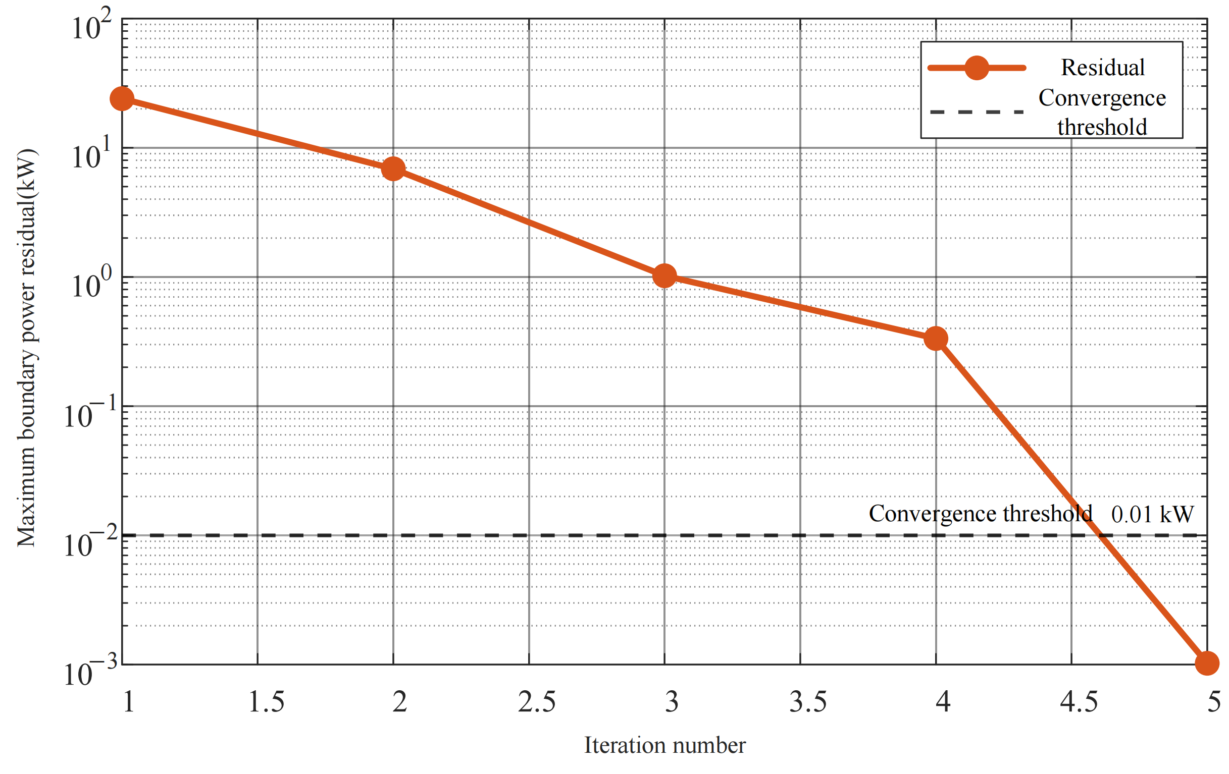
As shown in Figure 15, after five iterations, the boundary power residual of the ATC algorithm falls below the set threshold of 0.01 kW, with a monotonic downward convergence curve free from significant fluctuations, demonstrating excellent numerical stability. Throughout the iterative solution process, the ADN only needs to exchange limited coordination information—such as power target values and dual variables between boundary nodes—and requires no disclosure of internal resource allocation schemes, load demand data, equipment operating parameters, or cost functions for any microgrid. This design fundamentally safeguards commercial privacy and data security for all stakeholders, eliminates data leakage risks associated with centralized optimization that requires aggregating comprehensive network information, and better aligns with practical application scenarios involving collaborative scheduling between ADN operators and multiple independent microgrid owners. Overall, the ATC distributed algorithm achieves effective system privacy protection at minimal computational cost, validating its engineering applicability and practical value for coordinated distribution network–microgrid scheduling.

Figure 15. Convergence process of the ATC algorithm.

6. Conclusions

This study focuses on the coordinated optimal dispatch problem between distribution networks and multiple microgrids. A bi-level optimization framework for distribution network–microgrid systems is established, incorporating a load-side demand response mechanism and an ATC-based distributed solution algorithm to achieve economically efficient scheduling in multi-stakeholder scenarios. First, the structure of the distribution network system with microgrid integration is introduced, and the coordinated scheduling mechanism of power interaction between distribution networks and microgrids via interconnection lines is analyzed. A bi-level model is then developed, comprising upper-level active–reactive power coordination for the distribution network and lower-level multi-resource joint dispatch for microgrids. Second, a demand response mechanism is introduced at the microgrid level to fully exploit the active regulation potential of flexible loads through load shifting and load shedding. Third, the ATC distributed algorithm is employed to decompose and coordinatively solve the bi-level optimization problem, achieving a near-global optimal solution while safeguarding the information privacy of all stakeholders. Finally, the effectiveness of the proposed method is validated through multi-scenario comparative case studies, and the following main conclusions are drawn:

• The proposed distribution network–microgrid collaborative optimization framework can fully mobilize the active and reactive power regulation capabilities of distributed photovoltaics, energy storage systems, and reactive power compensation devices. Compared with independent ADN operation, collaborative optimization significantly reduces system network loss costs and total operating costs, while improving the voltage profile across all network nodes. This demonstrates that the integration of microgrids as active controllable units into distribution networks not only brings economic benefits but also provides voltage support.
• The introduction of load-side demand response within the collaborative optimization framework further reduces the total system operating costs. By curtailing and shifting flexible loads during high electricity price periods, the demand response mechanism optimizes the internal energy allocation structure of microgrids, leading to notable reductions in diesel generator fuel costs and pollutant emission costs. This enhances the active power support capability of microgrids to the distribution network and improves the environmental performance of distributed resources.
• The ATC-based distributed solution algorithm converges within a limited number of iterations, and the resulting total system operating cost deviates only marginally from the centralized global optimization solution, demonstrating satisfactory solution accuracy. Throughout the entire solution process, the ADN and each microgrid are required to exchange only limited coordination information, such as interconnection boundary power and Lagrange multipliers. The internal model parameters, device output strategies, and user load data of each stakeholder remain private, effectively safeguarding commercial information security and better meeting the practical application requirements of distributed collaborative scheduling involving multiple stakeholders in real-world engineering scenarios.

References

- Yan, M.; Shahidehpour, M.; Paaso, A.; Zhang, L.; Alabdulwahab, A.; Abusorrah, A. Distribution Network-Constrained Optimization of Peer-to-Peer Transactive Energy Trading among Multi-Microgrids. IEEE Trans. Smart Grid 2021, 12, 1033–1047. [Google Scholar] [CrossRef] [Scilit]
- Chen, Q.; Wang, W.Q.; Wang, H.Y. Coordinated Optimization of Active Distribution Network with Multiple Microgrids Considering Demand Response and Mixed Game. Autom. Electr. Power Syst. 2023, 47, 99–109. [Google Scholar]
- Wang, C.; Fang, R.C.; Lei, H.; Sun, J.J.; Cha, X.M. Day-Ahead and Intra-Day Collaborative Dispatching Method for Active Distribution Network Based on Optimal Economic Operation Region. Power Syst. Technol. 2024, 48, 1602–1617. [Google Scholar]
- Wu, W.C.; Lin, C.H.; Sun, H.B.; Wang, B.; Liu, H.T. Machine Learning-Based Energy Management and Operation Control for Active Distribution Networks. Autom. Electr. Power Syst. 2024, 48, 2–11. [Google Scholar]
- Chen, S.; Wang, C.; Zhang, Z. Multitime Scale Active and Reactive Power Coordinated Optimal Dispatch in Active Distribution Network Considering Multiple Correlation of Renewable Energy Sources. IEEE Trans. Ind. Appl. 2021, 57, 5614–5625. [Google Scholar] [CrossRef] [Scilit]
- Luo, J.; Liu, L.; Liu, P.; Ye, R.; Qin, P. An Optimal Scheduling Method for Active Distribution Network Considering Source-Network-Load-Storage Coordination. Power Syst. Prot. Control 2022, 50, 167–173. [Google Scholar]
- Nikmehr, N.; Ravadanegh, S.N. Optimal Power Dispatch of Multi-Microgrids at Future Smart Distribution Grids. IEEE Trans. Smart Grid 2015, 6, 1648–1657. [Google Scholar] [CrossRef] [Scilit]
- Zhang, X.X.; Niu, H.N.; Zhao, J.X. Optimal Dispatch Method of Distribution Network with Microgrid. Trans. China Electrotech. Soc. 2017, 32, 165–173. [Google Scholar]
- Li, X.; Fang, Z.; Li, F.; Xie, S.; Cheng, S. Game-Based Optimal Dispatching Strategy for Distribution Network with Multiple Microgrids Leasing Shared Energy Storage. Proc. CSEE 2022, 42, 6611–6625. [Google Scholar]
- Anoh, K.; Maharjan, S.; Ikpehai, A.; Zhang, Y.; Adebisi, B. Energy Peer-to-Peer Trading in Virtual Microgrids in Smart Grids: A Game Theoretic Approach. IEEE Trans. Smart Grid 2020, 11, 1264–1275. [Google Scholar] [CrossRef] [Scilit]
- Yang, W.W.; Peng, X.; Quan, H.; Chu, Z.; Wang, X.; Zhao, Z. Multi-Agent Game Collaborative Optimization Strategy for Active Distribution Networks Based on Federated Reinforcement Learning. Autom. Electr. Power Syst. 2025, 49, 70–82. [Google Scholar]
- Faheem, M.; Gungor, V.C. Capacity and spectrum-aware communication framework for wireless sensor network-based smart grid applications. Comput. Stand. Interfaces 2017, 53, 48–58. [Google Scholar] [CrossRef] [Scilit]
- Goswami, B.; Tian, Y.C.; Mishra, Y.; Jin, J.; Tang, Y. Communication Solutions for the Last Mile of Smart Grid: Neighborhood Area Networks in Smart Grid Communications: Standards and Challenges. IEEE Power Energy Mag. 2024, 22, 118–133. [Google Scholar] [CrossRef] [Scilit]
- Suhaimy, N.; Radzi, N.A.M.; Ahmad, W.S.H.M.W.; Azmi, K.H.M.; Hannan, M.A. Current and Future Communication Solutions for Smart Grids: A Review. IEEE Access 2022, 10, 43639–43668. [Google Scholar] [CrossRef] [Scilit]
- Rodriguez-Gil, J.A.; Mojica-Nava, E.; Vargas-Medina, D.; Arevalo-Castiblanco, M.F.; Cortes, C.A.; Rivera, S.; Cortes-Romero, J. Energy management system in networked microgrids: An overview. Energy Syst. 2026, 17, 315–346. [Google Scholar] [CrossRef] [Scilit]
- He, Q.Y.; Wang, J.R.; Yang, Y.B.; Xu, Q.S. Distributed Optimal Dispatch Model for Distribution Network with Multi-Microgrid Based on Alternating Direction Method of Multipliers. J. Electr. Eng. 2024, 19, 62–71. [Google Scholar]
- Ma, W.J.; Wang, J.; Gupta, V.; Chen, C. Distributed Energy Management for Networked Microgrids Using Online ADMM with Regret. IEEE Trans. Smart Grid 2018, 9, 847–856. [Google Scholar] [CrossRef] [Scilit]
- Marvasti, A.K.; Fu, Y.; DorMohammadi, S.; Rais-Rohani, M. Optimal Operation of Active Distribution Grids: A System of Systems Framework. IEEE Trans. Smart Grid 2014, 5, 1228–1237. [Google Scholar] [CrossRef] [Scilit]
- Xie, M.; Ji, X.; Ke, S.; Liu, M. Autonomous Optimized Economic Dispatch of Active Distribution Power System with Multi-Microgrids Based on Analytical Target Cascading Theory. Proc. CSEE 2017, 37, 4911–4921+5210. [Google Scholar]
- Zhao, B.; Wang, X.; Lin, D.; Calvin, M.M.; Morgan, J.C.; Qin, R.; Wang, C. Energy Management of Multiple Microgrids Based on a System of Systems Architecture. IEEE Trans. Power Syst. 2018, 33, 6410–6421. [Google Scholar] [CrossRef] [Scilit]
- Li, Y.; Ling, F.; Qiao, X.; Zhong, J.; Zhao, X.; Li, C.; Liu, J.; Xing, X.; Yang, K.; Lan, W. Mixed Game-Based Two-Stage Planning of PV and Energy Storage in Distribution System With Multiple Integrated Energy Microgrids. IEEE Trans. Ind. Appl. 2024, 60, 8054–8066. [Google Scholar] [CrossRef] [Scilit]
- Laws, N.D.; Hanasusanto, G.A. Linearizing Bilinear Products of Shadow Prices and Dispatch Variables in Bilevel Problems for Optimal Power System Planning and Operations. IEEE Trans. Power Syst. 2023, 38, 668–680. [Google Scholar] [CrossRef] [Scilit]
- Lin, Z.; Hu, Z.C.; Song, Y.H. A Review of Convex Relaxation Techniques for Optimal Power Flow Problems. Proc. CSEE 2019, 39, 3717–3728. [Google Scholar]
- Gao, H.J.; Liu, J.Y.; Shen, X.D.; Xu, R. Optimal Power Flow Research and Its Application in Active Distribution Networks. Proc. CSEE 2017, 37, 1634–1645. [Google Scholar]
- Mohammadi, A.; Mehrtash, M.; Kargarian, A. Diagonal Quadratic Approximation for Decentralized Collaborative TSO+DSO Optimal Power Flow. IEEE Trans. Smart Grid 2019, 10, 2358–2370. [Google Scholar] [CrossRef] [Scilit]
Disclaimer/Publisher’s Note: The statements, opinions and data contained in all publications are solely those of the individual author(s) and contributor(s) and not of MDPI and/or the editor(s). MDPI and/or the editor(s) disclaim responsibility for any injury to people or property resulting from any ideas, methods, instructions or products referred to in the content. |
© 2026 by the authors. Licensee MDPI, Basel, Switzerland. This article is an open access article distributed under the terms and conditions of the Creative Commons Attribution (CC BY) license.