Coordinated Planning and Scheduling of Rural Integrated-Energy Systems Considering Crop-Growth Requirements and Agricultural-Load Flexibility

Abstract

Facility agriculture couples energy operation with crop growth, yet existing studies often separate long-term capacity planning from short-term greenhouse scheduling. This paper develops a coordinated planning and 24 h day-ahead scheduling framework for a rural integrated-energy system with agricultural-load flexibility. The planning stage optimizes the capacities of the biogas generator, battery energy storage system (BESS), and gas boiler, while the existing 500 kW agrivoltaic photovoltaic (PV) system is treated as a sunk asset and kept fixed. The scheduling stage coordinates grid exchange, PV, biogas generation, BESS charging/discharging, supplementary-lighting regulation, and thermal supply under time-of-use tariffs, subject to PAR, DLI, GDD, indoor-temperature, and TDRW constraints. Compared with conventional seasonal planning, the proposed crop-growth-aware planning reduces annual planning cost by 9.01%. In day-ahead operation, agricultural flexibility alone reduces operating cost by 9.28%, while coordinated agricultural-load and BESS scheduling reduces it by 14.63%, increases PV utilization from 56.54% to 90.59%, and decreases daily operational carbon emissions from 4584.72 to 3817.39 kg CO₂·day⁻¹. These results quantify the distinct contributions of crop-constrained demand flexibility and storage while explicitly linking capacity decisions to short-term operation.

1. Introduction

The rapid electrification of modern agriculture is reshaping the structure and operation of rural energy systems [1]. Greenhouses, irrigation facilities, environmental control equipment, agricultural processing units, and other electrically driven devices are increasingly integrated with photovoltaic generation, bioenergy conversion, battery energy storage, and external power grids [2]. This transition improves the level of automation and renewable-energy utilization in agricultural production, but it also introduces stronger temporal coupling among electricity demand, thermal demand, crop growth, and environmental conditions. In particular, greenhouse lighting and heating loads are not purely conventional energy demands because their operating trajectories directly affect crop photosynthesis, temperature accumulation, biomass formation, and ultimately agricultural productivity [3]. Consequently, energy planning and operational scheduling in rural areas should not be conducted independently of crop physiological requirements.

Existing studies can be broadly divided into three streams. Rural integrated-energy planning studies optimize the type and capacity of distributed resources and usually evaluate operation only as an inner problem or representative-day check [4,5,6,7,8]. Greenhouse energy-management studies focus on operational control of lighting, heating, PV, and storage, but normally assume the installed capacities are already given [9,10,11,12,13,14,15]. Recent joint design-operation work has also shown the value of coordinating equipment sizing and operating decisions for greenhouse heating systems [16,17]. In parallel, load-scheduling studies for rural distributed generation have demonstrated techno-economic and environmental benefits, but do not impose cumulative crop-growth constraints such as DLI, GDD, and TDRW [18,19]. Therefore, the literature still lacks a framework that simultaneously links long-term capacity allocation, crop-constrained agricultural flexibility, and explicit day-ahead source-load-storage coordination.

A major challenge therefore lies in linking short-term energy scheduling with the cumulative physiological response of crops. The impacts of lighting and temperature on crop development are inherently time dependent. Instantaneous light intensity alone cannot fully characterize the effectiveness of greenhouse illumination [20,21], while instantaneous temperature cannot adequately represent the accumulated thermal conditions required for crop growth [22]. Agricultural indicators such as photosynthetically active radiation, daily light integral, growing degree-day, and daily dry-matter accumulation provide a more appropriate representation of these physiological requirements [23,24]. By embedding such indicators into energy optimization constraints, the flexibility of greenhouse loads can be exploited without sacrificing crop-growth performance [25].

Two gaps are particularly important. First, in many planning models the operational layer is used mainly to evaluate the feasibility and annual cost of a candidate capacity vector, rather than to examine how the planned resources should be coordinated hour by hour after installation [26]. Second, conventional demand-response formulations cannot be directly applied to greenhouse loads because temporal adjustment of lighting and heating changes the crop environment and accumulated physiological exposure. A planning scheme can therefore be economically attractive but operationally underutilize agricultural flexibility, whereas an operation-only model can implicitly rely on capacities that are not justified by a long-term planning decision. The present study addresses this planning-operation gap by passing the optimized equipment capacities explicitly to a separate 24 h scheduling model and by constraining agricultural flexibility with crop-growth indicators.

Battery energy storage further strengthens the need for coordinated scheduling. Unlike conventional generators, batteries are governed not only by instantaneous charging and discharging limits but also by intertemporal state-of-charge constraints. Their operational value depends on when energy is stored and released. Under time-of-use electricity prices, batteries can absorb renewable energy or low-cost grid electricity during favorable periods and discharge during high-price or high-demand periods [27]. When combined with agricultural-load flexibility, this creates a more complex coordination problem [15]. For example, greenhouse supplementary lighting may be flexibly regulated within an allowable physiological range, while storage may compensate for residual load variations [28]. The interaction between these two flexibility resources may reduce peak-grid demand, improve photovoltaic utilization [15], and lower operating costs. However, their contributions need to be quantitatively distinguished through comparative scheduling scenarios rather than inferred solely from planning results.

To address these gaps, this paper develops a two-stage coordinated planning and scheduling framework for rural integrated-energy systems considering crop-growth requirements and agricultural-load flexibility. The long-term stage determines equipment capacities using crop-growth-stage representative days; the day-ahead stage then fixes those capacities and optimizes grid exchange, distributed generation, BESS operation, supplementary lighting, and thermal supply. The existing 500 kW PV plant is excluded from the planning decision because it is a pre-installed asset in the studied village and its investment is therefore treated as sunk. The methodological contribution is not merely the aggregation of known components: the framework creates an explicit interface between crop-growth-aware capacity planning and post-planning operational coordination, and it separates the operating value of agricultural flexibility from that of battery storage under an identical planned capacity configuration.

The main contributions and research highlights are summarized as follows:

•

A crop-growth-aware planning–scheduling interface is established: representative-day planning determines equipment capacities, which are then transferred as fixed physical limits to an independent 24 h day-ahead scheduling problem.

•

Supplementary lighting is modeled as a flexible agricultural load constrained by instantaneous PAR and cumulative DLI, GDD, indoor-temperature, and TDRW requirements, thereby preventing purely economic load adjustment from violating prescribed crop-growth limits.

•

Agricultural flexibility and BESS flexibility are quantified separately through S1–S3 scenarios under the same capacity configuration, allowing their distinct contributions to operating cost, PV utilization, peak-grid demand, and operational carbon emissions to be identified.

•

A reproducibility-oriented case study reports hourly load/resource data, cost and emission parameters, PV curtailment, planning-cost decomposition, and sensitivity to tariff and PV-availability perturbations.

The remainder of the manuscript is organized as follows. Section 2 presents the physical model, planning objective, day-ahead scheduling formulation, data assumptions, and solution procedure. Section 3 reports the planning and scheduling results, sensitivity analysis, comparison with recent studies, and limitations. Section 4 summarizes the main conclusions and future research directions.

2. Materials and Methods

2.1. Physical Model of the Rural Integrated-Energy System

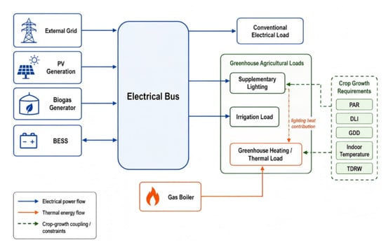
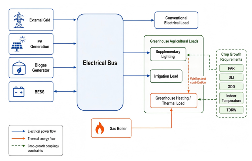
The overall energy-flow structure of the studied system is illustrated in Figure 1, with the corresponding configuration also provided in Figure S1 in the Supplementary Materials. PV generation, the biogas generator, the external grid, and BESS are coupled through the electrical bus, while the gas boiler supplies the greenhouse thermal demand. Supplementary lighting acts as a key coupling variable because it simultaneously affects electrical consumption, crop-light conditions, and the internal heat gain of the greenhouse.

Figure 1. Configuration of the rural integrated-energy system for coordinated planning and scheduling.

The rural integrated-energy system consists of an external power grid, an existing agrivoltaic PV system, a biogas generator, a BESS, a gas boiler, greenhouse agricultural loads, and conventional rural loads. The 500 kW PV plant was already installed before the planning study; consequently, its investment is sunk and PV capacity is treated as a fixed parameter rather than a planning decision. The scheduling horizon is divided into 24 one-hour intervals. The BESS energy capacity used in the scheduling extension is 972 kWh, corresponding to a 2 h duration at the planned 486 kW power rating.

t = 1,2,…,24,  Δt = 1 h

(1)

The total agricultural electrical load is expressed as (2), where $P_t^{\mathrm{light}}$ and $P_t^{\mathrm{ir}}$ are the supplementary lighting and irrigation loads, respectively. The actual supplementary-lighting demand is expressed as (3), where $P_t^{\mathrm{light},0}$ is the baseline lighting demand, and $P_t^{\mathrm{up}}$ and $P_t^{\mathrm{down}}$ denote upward and downward load regulation. The regulation limits are (4).

$$P_t^{\mathit{agri}}=P_t^{\mathrm{light}}+P_t^{\mathrm{ir}}$$

(2)

$$P_t^{\mathrm{light}}=P_t^{\mathrm{light},0}+P_t^{\mathrm{up}}-P_t^{\mathrm{down}}$$

(3)

$$\left\{\begin{array}{c}0\le P_t^{\mathrm{up}}\le P_{{\max }^{\mathrm{up}}}\\ 0\le P_t^{\mathrm{down}}\le P_t^{\mathrm{light},0}\end{array}\right.$$

(4)

The total photosynthetically active radiation (PAR) received by the crop is represented as the sum of natural solar PAR and supplementary-lighting PAR in (5) [29]. The lighting-induced component is related to electrical lighting power by (6). In the case study, the aggregate conversion coefficient is set to κ_PAR = 1.20 μmol·m⁻²·s⁻¹·kW⁻¹. This coefficient is a calibrated greenhouse-level surrogate chosen to reproduce the baseline daily light integral; it should not be interpreted as a fixture-level photon efficacy because the effective PAR at canopy level depends on lamp technology, spectrum, mounting geometry, and crop canopy characteristics. The instantaneous PAR bounds in (7) are imposed for the selected pepper growth stage.

$$R_t^{\mathrm{PAR}}=R_t^{\mathrm{sun},\mathrm{PAR}}+R_t^{\mathrm{light},\mathrm{PAR}}$$

(5)

$$R_t^{\mathrm{light},\mathrm{PAR}}={\kappa }_{\mathrm{PAR}}{P}_t^{\mathrm{light}}$$

(6)

$$R_{\mu }^{\min }\le R_{\mu ,t}^{\mathrm{PAR}}\le R_{\mu }^{\max }$$

(7)

The daily light integral (DLI) is defined by (8) and constrained by (9). For the pepper growth stage, DLI is limited to 10–20 mol·m⁻²·d⁻¹, while the instantaneous PAR range is 35–1791 μmol·m⁻²·s⁻¹, following the crop-growth requirements adopted in [4]. The gross greenhouse thermal requirement in (10) aggregates envelope/ground heat losses and ventilation/infiltration losses, minus useful solar gains. In the scheduling extension, these terms are not re-identified separately; their net effect is calibrated to the representative-day greenhouse heating profile reported in [4]. This approach avoids introducing unverified envelope parameters while retaining the hourly thermal-demand trajectory.

$${\mathrm{DLI}}_{\mu }={\displaystyle \frac{3600\Delta t}{{10}^6}}{\displaystyle {\displaystyle \sum }_{t=1}^{24}}{R}_{\mu ,t}^{\mathrm{PAR}}$$

(8)

$${\mathrm{DLI}}_{\mu }^{\min }\le {\mathrm{DLI}}_{\mu }\le {\mathrm{DLI}}_{\mu }^{\max }$$

(9)

$$L_t^{\mathrm{h}}=Q_t^{\mathrm{loss}}-Q_t^{\mathrm{sun}}$$

(10)

The lighting-derived heat in (11) is represented using an equivalent lighting-to-heat coefficient κ_h = 0.55 kW_th/kW_e. This coefficient represents the fraction of electrical lighting power ultimately released as sensible heat to the greenhouse in the aggregate scheduling model and is used as a calibrated surrogate rather than a universal lamp property. Greenhouse thermal inertia is considered through a first-order temperature-deviation model around the baseline profile: the next-hour temperature deviation depends on the previous deviation and on deviations of boiler heat and lighting power from their baseline values. The calibrated coefficients are a = 0.88, b_H = 0.012 °C/(kW·h), and b_L = 0.0066 °C/(kW·h). The indoor temperature is therefore dynamically coupled across hours rather than determined independently. GDD is constrained to 10–20 °C·d, indoor temperature to 10–35 °C, and TDRW to at least 180 kg·hm⁻²·d⁻¹ for pepper [4]. TDRW is used here as a calibrated daily biomass proxy; satisfying these indicators does not by itself guarantee realized crop yield, a limitation discussed in Section 3.8.

$$Q_t^{\mathrm{light}}={\kappa }_{\mathrm{h}}{P}_t^{\mathrm{light}}$$

(11)

$$T_{\mu }^{\min }\le T_t^{\mathrm{in}}\le T_{\mu }^{\max }$$

(12)

$${\mathrm{GDD}}_{\mu }={\displaystyle {\displaystyle \sum }_{t=1}^{24}}{\psi }_{\mu }\left(T_t^{\mathrm{in}}\right){\displaystyle \frac{\Delta t}{24}}$$

(13)

$${\psi }_{\mu }(T_t^{\mathit{in}})=\left\{\begin{array}{c}0,T_t^{\mathit{in}}\le T_{\mu }^{\mathit{iase}}\\ T_t^{\mathit{in}}-T_{\mu }^{\mathit{base}},T_{\mu }^{\mathit{base}}<T_t^{\mathit{in}}\le T_{\mu }^{\mathit{opt}}\\ {\displaystyle \frac{T_{\mu }^{\mathit{max}}-T_t^{\mathit{in}}}{T_{\mu }^{\mathit{max}}-T_{\mu }^{\mathit{opt}}}}\left(T_{\mu }^{\mathit{opt}}-T_{\mu }^{\mathit{base}}\right),T_{\mu }^{\mathit{apt}}<T_t^{\mathit{in}}<T_{\mu }^{\mathit{max}}\\ 0,T_t^{\mathit{in}}\ge T_{\mu }^{\mathit{max}}\end{array}\right.$$

(14)

$${\mathrm{GDD}}_{\mu }^{\min }\le {\mathrm{GDD}}_{\mu }\le {\mathrm{GDD}}_{\mu }^{\max }$$

(15)

$$\left\{\begin{array}{c}\mathit{TDR}{W}_{\mu }={\xi }_{\mu }\mathit{DL}{I}_{\mu }\\ \mathit{TDR}{W}_{\mu }\ge \mathit{TDR}{W}_{\mu }^{\mathit{min}}\end{array}\right.$$

(16)

The electrical power balance of the rural integrated-energy system is (17) and part of this thermal requirement can be supplied by the heat released from supplementary lighting. Therefore, the greenhouse thermal balance is expressed as (18), while the external-grid power is constrained by (19). The utilized PV output satisfies (20) and the curtailed PV power is (21). The biogas-generator output is constrained by (22) while its ramping capability is described by (23).

$$P_t^{\mathrm{grid}}+P_t^{\mathrm{PV}}+P_t^{\mathrm{BG}}+P_t^{\mathrm{dis}}=L_t^{\mathrm{base}}+P_t^{\mathrm{agri}}+P_t^{\mathrm{ch}}$$

(17)

$$H_t^{\mathrm{GB}}+Q_t^{\mathrm{light}}=L_t^{\mathrm{h}}$$

(18)

$$0\le P_t^{\mathrm{grid}}\le P_{\mathrm{grid}}^{\max }$$

(19)

$$0\le P_t^{\mathrm{PV}}\le {\widehat{P}}_t^{\mathrm{PV}}$$

(20)

$$P_t^{\mathrm{cur}}={\widehat{P}}_t^{\mathrm{PV}}-P_t^{\mathrm{PV}}$$

(21)

$$0\le P_t^{\mathrm{BG}}\le {\mathrm{Cap}}_{\mathrm{BG}}^{\mathrm{opt}}$$

(22)

$$-R_{\mathrm{BG}}^{\mathrm{down}}\le P_t^{\mathrm{BG}}-P_{t-1}^{\mathrm{BG}}\le R_{\mathrm{BG}}^{\mathrm{up}}$$

(23)

The gas-boiler output satisfies (24) and the BESS charging and discharging powers satisfy (25), while simultaneous charging and discharging are prohibited by (26).

$$0\le H_t^{\mathrm{GB}}\le {\mathrm{Cap}}_{\mathrm{GB}}^{\mathrm{opt}}$$

(24)

$$\left\{\begin{array}{c}0\le P_t^{\mathrm{ch}}\le u_t^{\mathrm{ch}}{P}_{\max }^{\mathrm{ch}}\\ 0\le P_t^{\mathrm{dis}}\le u_t^{\mathrm{dis}}{P}_{\max }^{\mathrm{dis}}\end{array}\right.$$

(25)

$$u_t^{\mathrm{ch}}+u_t^{\mathrm{dis}}\le 1$$

(26)

The battery energy state evolves according to (27) and the stored energy satisfies (28). The state of charge is (29) and the terminal energy state is constrained as (30), which ensures that the scheduling benefit is not obtained by simply depleting the battery at the end of the scheduling horizon.

The BESS representation separates long-term capacity cost from short-term cycling cost. In planning, BESS investment and annual maintenance are charged through the annualized capacity terms. In day-ahead scheduling, an additional equivalent degradation cost of 0.03 CNY·kWh⁻¹ of charge-plus-discharge throughput is applied to discourage unnecessary cycling. This linear throughput cost is a computationally tractable proxy for cycle aging; detailed dependence on depth of discharge, temperature, and cycle history is not modeled.

$$E_t=E_{t-1}+{\eta }_{\mathrm{ch}}{P}_t^{\mathrm{ch}}\Delta t-{\displaystyle \frac{P_t^{\mathrm{dis}}\Delta t}{{\eta }_{\mathrm{dis}}}}$$

(27)

E^min ≤ E_t ≤ E^max

(28)

$$\left\{\begin{array}{c}{\mathrm{SOC}}_t={\displaystyle \frac{E_t}{E^{\mathrm{rated}}}}\\ {\mathrm{SOC}}^{\min }\le {\mathrm{SOC}}_t\le {\mathrm{SOC}}^{\max }\end{array}\right.$$

(29)

E₂₄ = E₀

(30)

2.2. Planning Objective Function

The long-term planning decision vector is defined in (31) and the capacity limits in (32). The planning objective minimizes the equivalent annual cost in (33), including annualized investment, annual maintenance, and annual operating cost. The planning horizon is 15 years, the fixed-asset residual rate is 5%, and the discount rate is 8%, consistent with the validated planning case in [4]. The unit investment costs are 500 CNY/kW for the biogas generator, 1446 CNY/kW for the BESS, and 672 CNY/kW for the gas boiler; the corresponding annual maintenance coefficients are 10, 10, and 20 CNY·kW⁻¹·year⁻¹, respectively [4]. The capital recovery factor is calculated by (35).

x^pl = [Cap_BG,Cap_BT,Cap_GB]

(31)

$$0\le {\mathrm{Cap}}_i\le {\mathrm{Cap}}_i^{\max },i\in {\mathsf{\Omega }}^{\mathrm{pl}}$$

(32)

minF^pl = F^inv + F^main + F^ope

(33)

$$F^{\mathrm{inv}}={\displaystyle \sum }_{i\in {\mathsf{\Omega }}^{\mathrm{pl}}}{\mathrm{CRF}}_i{C}_i{\mathrm{Cap}}_i$$

(34)

$${\mathrm{CRF}}_i={\displaystyle \frac{r{\left(1+r\right)}^{Y_i}}{{\left(1+r\right)}^{Y_i}-1}}$$

(35)

The annual operating cost in (37) is obtained by weighting representative-day operating costs by the number of calendar days in the corresponding crop-growth stage. Eight representative stages are used, with weights Ds = {9, 65, 66, 8, 102, 7, 48, 60} days for pepper germination, pepper growth stage 1, pepper growth stage 2, tomato germination, tomato growth, cucumber germination, cucumber growth stage 1, and cucumber growth stage 2, respectively; the weights sum to 365 days. This crop-growth-stage weighting is the key difference from the conventional seasonal benchmark, which selects representative days by season rather than by crop physiological stage.

$$F^{\mathrm{main}}={\displaystyle \sum }_{i\in {\mathsf{\Omega }}^{\mathrm{pl}}}{c}_i^{\mathrm{main}}{\mathrm{Cap}}_i$$

(36)

$$F^{\mathrm{ope}}={\displaystyle \sum }_{s\in \mathcal{S}}{D}_s{F}_s^{\mathrm{day}}$$

(37)

$$F_s^{\mathrm{day}}=\underset{x_s^{\mathrm{op}}}{\min }{f}_s^{\mathrm{op}}\left(x_s^{\mathrm{op}},x^{\mathrm{pl}}\right)$$

(38)

$$\left\{\begin{array}{c}g\left(x_s^{\mathrm{op}},x^{\mathrm{pl}}\right)=0\\ h\left(x_s^{\mathrm{op}},x^{\mathrm{pl}}\right)\le 0\end{array}\right.$$

(39)

After the planning problem is solved, the optimal equipment capacities are fixed and transferred to the day-ahead scheduling stage:

$${\mathrm{Cap}}_i={\mathrm{Cap}}_i^{\mathrm{opt}}$$

(40)

This planning-operation linkage ensures that short-term scheduling is conducted within the physical boundaries determined by long-term capacity allocation.

2.3. Day-Ahead Scheduling Objective Function

With the planned capacities fixed, the day-ahead scheduling problem minimizes the total operating cost:

minF^sch = F^grid + F^BG + F^GB + F^DR + F^BT

(41)

The grid-purchasing, biogas-generation, gas-boiler, agricultural-regulation, and BESS-throughput costs are given by (42)–(46). The operating coefficients used in the case study are 0.48 CNY·kWh⁻¹ for biogas generation, 0.32 CNY·kWh⁻¹ for the gas boiler, 0.05 CNY·kWh⁻¹ for lighting regulation, and 0.03 CNY·kWh⁻¹ for BESS throughput [30,31]. Carbon emissions are not included in the scheduling objective; they are calculated after optimization as a performance indicator. A single economic objective is retained to avoid introducing subjective weighting coefficients between cost, peak demand, and emissions and to make the separate effects of agricultural flexibility and BESS easier to interpret. Peak-grid power and carbon emissions are therefore reported ex post.

$$F^{\mathrm{grid}}={\displaystyle {\displaystyle \sum }_{t=1}^{24}}{c}_t^{\mathrm{grid}}{P}_t^{\mathrm{grid}}\Delta t$$

(42)

$$F^{\mathrm{BG}}={\displaystyle {\displaystyle \sum }_{t=1}^{24}}{c}^{\mathrm{BG}}{P}_t^{\mathrm{BG}}\Delta t$$

(43)

$$F^{\mathrm{GB}}={\displaystyle {\displaystyle \sum }_{t=1}^{24}}{c}^{\mathrm{GB}}{H}_t^{\mathrm{GB}}\Delta t$$

(44)

$$F^{\mathrm{DR}}={\displaystyle {\displaystyle \sum }_{t=1}^{24}}{c}^{\mathrm{DR}}\left(P_t^{\mathrm{up}}+P_t^{\mathrm{down}}\right)\Delta t$$

(45)

$$F^{\mathrm{BT}}={\displaystyle {\displaystyle \sum }_{t=1}^{24}}{c}^{\mathrm{BT}}\left(P_t^{\mathrm{ch}}+P_t^{\mathrm{dis}}\right)\Delta t$$

(46)

$$C_t^{\mathrm{em}}={\lambda }_{\mathrm{grid}}{P}_t^{\mathrm{grid}}\Delta t+{\lambda }_{\mathrm{BG}}{P}_t^{\mathrm{BG}}\Delta t+{\lambda }_{\mathrm{GB}}{H}_t^{\mathrm{GB}}\Delta t$$

(47)

The total daily operational carbon emission is calculated by (48) [32,33,34]. The case-study emission factors are 0.57 kg CO₂·kWh⁻¹ for grid electricity, 0.10 kg CO₂·kWh⁻¹ for biogas generation, and 0.20 kg CO₂·kWhₜₕ⁻¹ for gas-boiler heat. These factors are used as direct operational accounting coefficients for scenario comparison; upstream fuel production, equipment manufacturing, construction, and other life-cycle emissions are not included. Hence, the reported values should be interpreted as operational rather than life-cycle carbon emissions.

$$C^{\mathrm{day}}={\displaystyle {\displaystyle \sum }_{t=1}^{24}}{C}_t^{\mathit{em}}$$

(48)

The complete coordinated scheduling problem is compactly expressed as (49), where Ω_energy represents the electrical and thermal balance constraints and operating limits of distributed energy resources, Ω_BESS represents the intertemporal battery constraints, and Ω_agri denotes the feasible agricultural flexibility region determined by PAR, DLI, greenhouse temperature, GDD, and TDRW requirements.

For reproducibility, PV utilization is defined as the ratio of total utilized PV energy to total available PV energy over the 24 h horizon. Curtailed PV energy is defined as the time integral of the difference between available and utilized PV power. Because no load-shedding variable is included and hourly electrical/thermal balance is enforced, the deterministic scenarios have zero unserved energy whenever the optimization is feasible.

$$\left\{\begin{array}{c}\underset{x^{\mathrm{sch}}}{\min }{F}^{\mathrm{sch}}\\ x^{\mathrm{sch}}\in {\mathsf{\Omega }}_{\mathrm{energy}}\cap {\mathsf{\Omega }}_{\mathrm{BESS}}\cap {\mathsf{\Omega }}_{\mathrm{agri}}\end{array}\right.$$

(49)

The proposed formulation links long-term distributed energy planning with short-term source-load-storage scheduling. Agricultural-load flexibility is utilized only within the physiologically feasible crop-growth region, while battery storage provides additional intertemporal flexibility for reducing grid dependence, supporting potential peak-demand management, and improving renewable-energy utilization.

2.4. Solution Procedure and Reproducibility

The long-term model retains the bilevel solution structure of the validated planning framework [4]: particle swarm optimization searches the upper-level capacity vector, and Gurobi solves the lower-level operational problem for each candidate. The new 24 h scheduling extension is formulated as a mixed-integer linear program because charging and discharging mode variables are binary and all remaining relations are linear or linearized. The scheduling model is implemented in MATLAB/YALMIP and solved with Gurobi 10.0.1. The relative MIP optimality tolerance is 10⁻⁴; all three S1–S3 scheduling cases reached an optimal solution. The computational procedure is: (i) read capacities and representative-day data; (ii) construct energy, BESS, and crop-growth constraints; (iii) solve the selected scenario; (iv) calculate cost, PV utilization, peak demand, carbon emissions, and crop indicators; and (v) compare scenarios under identical planned capacities.For clarity, the main variables, parameters, and their units used in the mathematical formulation are summarized in Appendix B.

3. Results and Discussion

3.1. Case Description and Parameter Settings

The proposed framework is evaluated on a rural integrated-energy system containing the grid, an existing 500 kW agrivoltaic PV plant, a biogas generator, BESS, gas boiler, conventional rural electrical load, and greenhouse loads. Table 1 summarizes the parameters used to reproduce the case study, while the detailed system scheduling parameters are also provided in Table S1 in the Supplementary Materials. Parameters inherited from the validated rural planning case [4] are distinguished from scheduling-extension assumptions in the accompanying source note. The transformer limit is 900 kW. The planned capacities subsequently used in all scheduling cases are 172 kW for the biogas generator, 486 kW/972 kWh for the BESS, and 1090 kW for the gas boiler.

Table 1. System, economic, emission, and scheduling parameters.

Parameter	Value
Transformer capacity (kW)	900
PV-installed capacity (kW)	500
Biogas-generator capacity (kW)	172
BESS power capacity (kW)	486
Gas-boiler capacity (kW)	1090
Initial SOC (%)	50
Minimum SOC (%)	20
Maximum SOC (%)	90
Charging efficiency	0.95
Discharging efficiency	0.95
Valley electricity price (CNY·kWh−1)	0.35
Flat electricity price (CNY·kWh−1)	0.62
Peak electricity price (CNY·kWh−1)	1.05
DLI range (mol·m−2·d−1)	10–20
GDD range (°C·d)	10–20
Minimum TDRW (kg·hm−2·d−1)	180
PAR range (μmol·m−2·s−1)	35–1791
Greenhouse temperature range (°C)	10–35
BESS energy capacity (kWh)	972
Biogas ramp limit (kW·h−1)	60
Biogas-generation cost (CNY·kWh−1)	0.48
Gas-boiler operating cost (CNY·kWhₜₕ−1)	0.32
Lighting-regulation cost (CNY·kWh−1)	0.05
BESS degradation/throughput cost (CNY·kWh−1)	0.03
Biogas unit investment cost (CNY·kW−1)	500
BESS unit investment cost (CNY·kW−1)	1446
Gas-boiler unit investment cost (CNY·kW−1)	672
Biogas annual maintenance (CNY·kW−1·year−1)	10
BESS annual maintenance (CNY·kW−1·year−1)	10
Gas-boiler annual maintenance (CNY·kW−1·year−1)	20
Planning horizon (year)	15
Discount rate (%)	8
Residual value rate (%)	5
PAR conversion coefficient κPAR (μmol·m−2·s−1·kW−1)	1.20
Lighting-to-heat coefficient κh (kWth/kWe)	0.55
Thermal-inertia coefficient a	0.88
Thermal coefficient bH [°C/(kW·h)]	0.012
Thermal coefficient bL [°C/(kW·h)]	0.0066
Grid emission factor (kg CO2·kWh−1)	0.57
Biogas emission factor (kg CO2·kWh−1)	0.10
Gas-boiler emission factor (kg CO2·kWhₜₕ−1)	0.20

Source note: transformer/PV capacities, planned device capacities, crop-growth ranges, investment/maintenance parameters, and the planning horizon follow the validated case in [4]. The TOU tariff, BESS energy duration and SOC limits, operating/degradation costs, aggregate PAR conversion, thermal-inertia coefficients, and operational emission factors are explicit assumptions of the day-ahead scheduling extension.

The 24 h scheduling illustration uses the second representative day, corresponding to the pepper growth stage, because this stage simultaneously activates supplementary lighting, irrigation, and greenhouse heating and therefore exposes the strongest electricity–heat–crop coupling. The scheduling interval is 1 h. The BESS initial SOC is 50%, with lower/upper bounds of 20% and 90%, charging/discharging efficiencies of 95%, and terminal SOC fixed to its initial value. The complete 24 h input profiles for conventional electrical load, supplementary lighting, irrigation, heating, and available PV power are reported in Appendix A. The pepper-day result is used to demonstrate the day-ahead mechanism, whereas the annual planning stage uses all eight crop-growth-stage representative days described in Section 2.2.

Three scheduling scenarios are considered. In S1, agricultural loads follow their baseline profiles and the BESS is disabled. In S2, supplementary lighting is treated as a flexible agricultural load, while BESS operation remains disabled. In S3, both agricultural flexible loads and the BESS participate in coordinated scheduling. The three scenarios are therefore used to progressively evaluate the benefits of conventional operation, agricultural demand flexibility, and source-load-storage coordination.

3.2. Planning Results and Capacity Configuration

To demonstrate the planning contribution, the proposed crop-growth-stage representative-day method is compared with a conventional seasonal planning benchmark. Both cases use the same candidate equipment set, investment/maintenance parameters, capacity limits, and lower-level energy-balance constraints. The difference is scenario construction: the conventional case uses seasonal representative days, whereas the proposed case uses representative days aligned with crop physiological stages and their 365-day weights. Thus, the planning comparison isolates the effect of crop-growth-aware scenario selection rather than changing the equipment technology set.

Compared with conventional planning, the proposed method reduces the required capacities of the biogas generator and gas boiler from 298 kW and 1180 kW to 172 kW and 1090 kW, respectively, while increasing the BESS power capacity from 289 kW to 486 kW. This capacity redistribution indicates that part of the conventional dispatchable-generation requirement is replaced by greater storage flexibility.

The annual planning cost decreases from 23.08 × 10⁵ CNY under conventional planning to 21.00 × 10⁵ CNY under the proposed strategy, a reduction of 9.01%. Table 2 now decomposes this total into annualized investment, annual maintenance, and annual operating cost. The proposed plan increases annualized investment slightly because it installs more BESS power, but this is more than offset by lower annual operating cost; therefore, operating-cost reduction is the dominant source of the net planning benefit.

Table 2. Comparison of planning results.

Indicator	Conventional Planning	Proposed Planning
Biogas-generator capacity (kW)	298	172
BESS power capacity (kW)	289	486
Gas-boiler capacity (kW)	1180	1090
Annualized investment cost (×105 CNY)	1.51	1.69
Annual maintenance cost (×105 CNY)	0.29	0.28
Annual operating cost (×105 CNY)	21.28	19.03
Total annual planning cost (×105 CNY)	23.08	21.00
Planning-cost reduction relative to conventional planning (%)	0.00	9.01

The optimized capacities of 172 kW for the biogas generator, 486 kW for the BESS, and 1090 kW for the gas boiler are subsequently fixed as the equipment limits in the day-ahead scheduling model. In this manner, the planning and scheduling stages are explicitly linked: the planning stage determines the available resource boundaries, whereas the scheduling stage evaluates how the planned resources are coordinated during actual operation.

This planning-operation linkage is essential to the proposed framework because the following S1–S3 comparison is performed under the capacity configuration determined by the planning stage rather than under arbitrarily selected equipment capacities.

3.3. Electrical Power Scheduling Characteristics

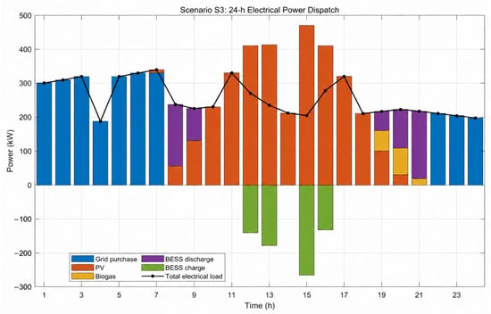
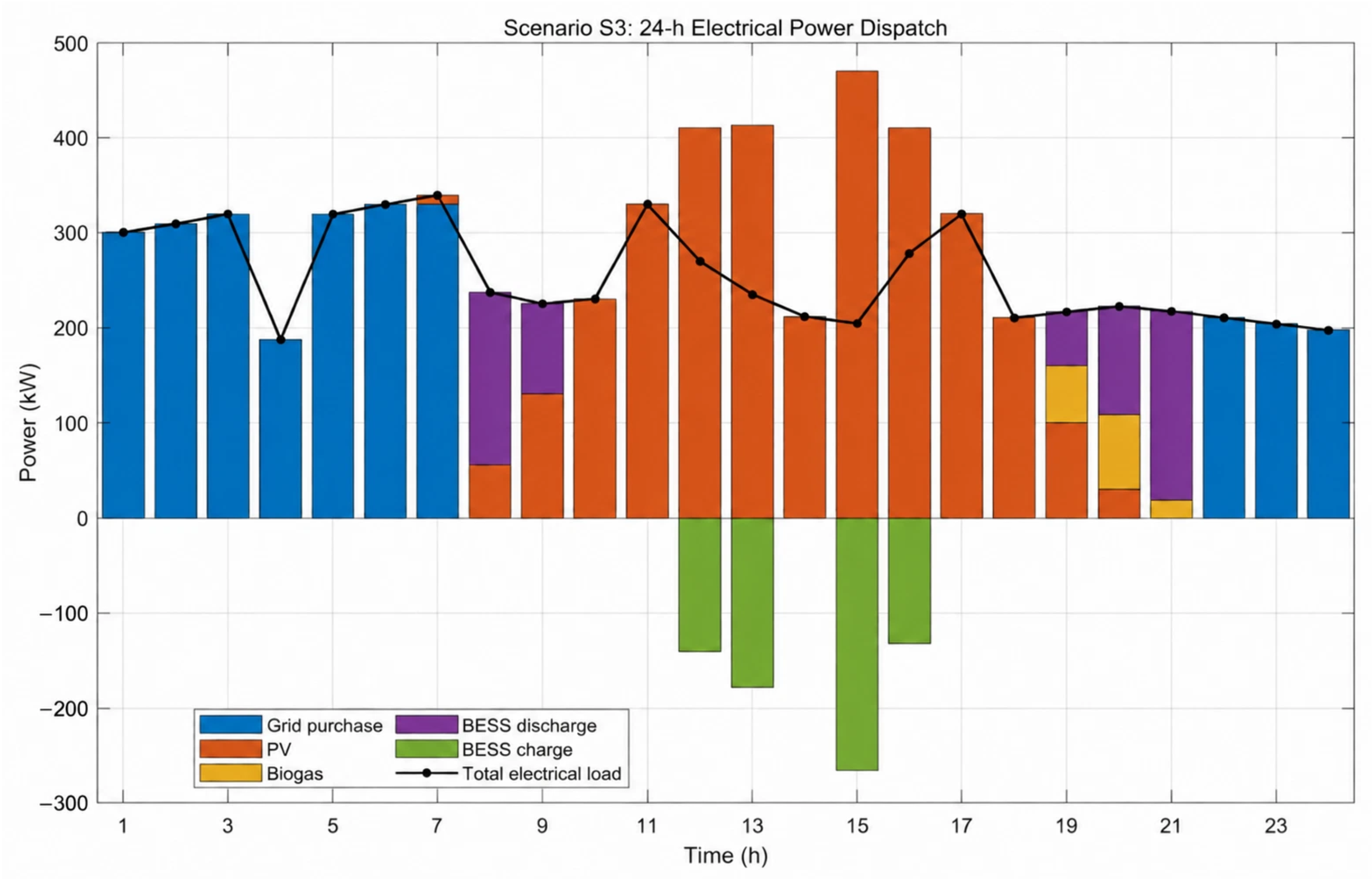
Figure 2 presents the 24-h electrical power dispatch result under S3, and the corresponding result is also provided in Figure S2 in the Supplementary Materials. The external grid, PV generation, biogas generation, and BESS jointly satisfy the time-varying electrical demand. A pronounced temporal complementarity can be observed among these resources.

Figure 2. 24 h electrical power dispatch under Scenario S3.

During the early-morning period, PV generation is unavailable and the electrical demand is mainly supplied by the external grid. From approximately 8:00 onward, PV generation gradually becomes the dominant power source. Around noon, PV generation exceeds the instantaneous load requirement. Instead of curtailing this surplus renewable generation, the BESS absorbs part of the available PV energy through charging. In particular, relatively high charging power can be observed around 12:00–16:00, corresponding to the period of abundant solar generation.

During the evening period, PV generation rapidly decreases, while agricultural and conventional loads remain considerable. The BESS therefore switches to discharging mode and supplies part of the demand, together with the biogas generator, thereby reducing the dependence on external-grid electricity. These results demonstrate that the proposed scheduling model enables an explicit temporal coordination among renewable generation, flexible agricultural demand, and storage operation.

It should be noted that battery charging power is plotted as a negative value in Figure 2, whereas generation and battery discharging are shown as positive values. This representation directly illustrates the charging and discharging states of the BESS and facilitates the interpretation of system-level electrical power balance. Additional electrical scheduling results are provided in Figure S1 in the Supplementary Materials.

3.4. BESS Charging/Discharging and SOC Evolution

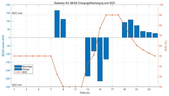
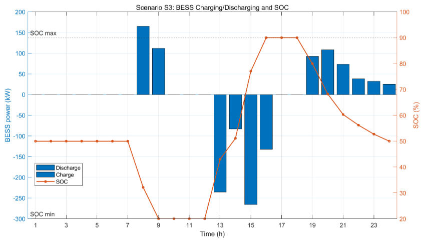
The detailed BESS operation is shown in Figure 3, with the corresponding BESS power and SOC results also provided in Figure S3 in the Supplementary Materials. The battery SOC starts from 50% and remains within the prescribed interval of 20–90% throughout the scheduling horizon. The battery discharges during several periods with relatively high net load and subsequently absorbs surplus PV energy during the daytime.

Figure 3. BESS charging/discharging power and SOC trajectory under Scenario S3.

From 8:00 to 9:00, battery discharging causes the SOC to decrease from approximately 50% to its lower limit of 20%. During the high-PV period from approximately 12:00 to 16:00, the battery is charged and the SOC gradually increases to approximately 90%. During the evening load period, the stored energy is released again, causing the SOC to decrease. Finally, the SOC returns to 50% at the end of the scheduling horizon, satisfying the terminal energy constraint.

The SOC trajectory indicates that the economic benefit of the BESS is achieved through intertemporal energy transfer rather than net energy depletion. In addition, no simultaneous charging and discharging occurs, demonstrating that the mutually exclusive operating constraints are correctly enforced.

Operation at the 20% and 90% SOC bounds is economically optimal for the present deterministic price/PV profile because the model exploits the full usable energy window when it creates net operating-cost savings. However, frequent operation near SOC extremes can accelerate battery aging in practice. The throughput-based degradation term in (46) partially internalizes cycling cost, but it does not capture the nonlinear dependence of aging on SOC, depth of discharge, temperature, and cycle history. This is therefore treated as a model limitation rather than evidence that persistent boundary operation is universally desirable.

The BESS mainly performs two functions in the proposed system. First, it absorbs renewable electricity during high-PV periods and improves local PV accommodation. Second, it transfers stored energy to subsequent high-demand periods, thereby reducing the amount of expensive external electricity that must be purchased.

3.5. Agricultural Flexible-Load Regulation

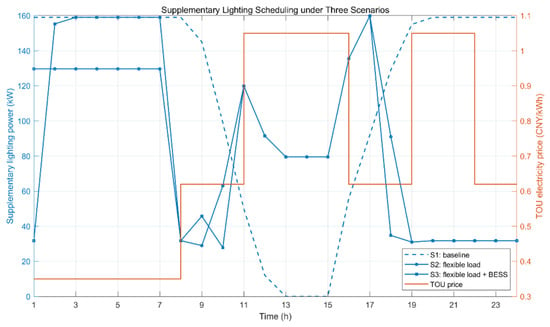
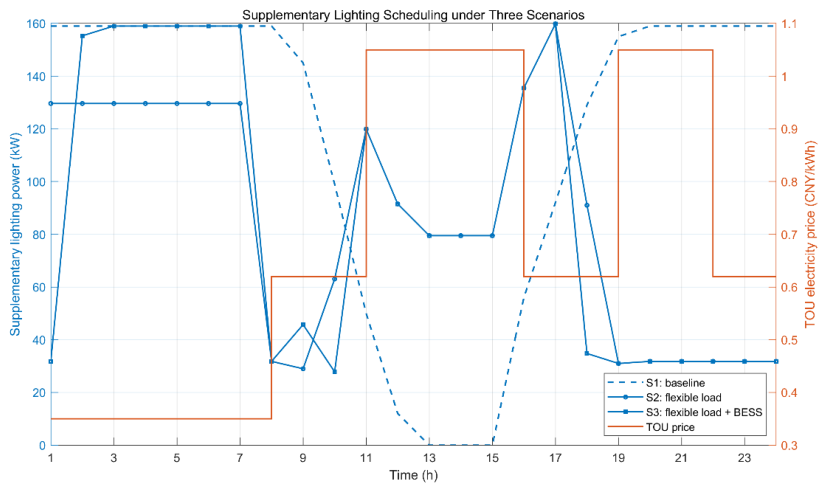
The supplementary lighting profiles under the three scenarios are compared in Figure 4, together with the TOU electricity price; the corresponding lighting comparison is also provided in Figure S4 in the Supplementary Materials. A clear difference can be observed between the fixed-load case S1 and the flexible-load cases S2 and S3.

Figure 4. Flexible regulation of supplementary lighting under the three scenarios and corresponding TOU electricity price.

Under S1, supplementary lighting follows the baseline agricultural demand profile and does not respond to electricity prices or renewable generation. In contrast, S2 and S3 allow the lighting demand to be temporally redistributed within the feasible crop-growth region. Consequently, the supplementary-lighting demand is adaptively adjusted in response to electricity prices and renewable-energy availability while satisfying the prescribed crop-growth constraints.

The results also indicate that the optimized lighting profiles of S2 and S3 are relatively similar. This is expected because the agricultural growth constraints determine the feasible redistribution range of the lighting load, whereas the BESS mainly provides energy-side flexibility. Therefore, the addition of BESS in S3 does not necessarily produce a substantial further change in the crop-light schedule after the available agricultural-load flexibility has already been utilized in S2.

The optimization results show that the lighting-regulation amount reaches approximately 908.98 kWh·day⁻¹ in both flexible scheduling scenarios. Nevertheless, the load redistribution does not violate the crop-growth constraints. The DLI decreases from 16.09 mol/(m²·d) in S1 to approximately 12.86 mol/(m²·d) in S2 and S3, which remains within the allowable range of 10–20 mol/(m²·d). The corresponding GDD is approximately 12.96 °C·d, also satisfying its admissible range.

The TDRW value decreases from approximately 225.21 kg/(hm²·d) in S1 to 180.00 kg/(hm²·d) in S2 and S3. This result indicates that the optimization fully exploits the available agricultural flexibility and drives the crop-growth state close to the lower feasible boundary. Therefore, although the current results demonstrate mathematical feasibility, an additional agricultural safety margin can be introduced in practical applications to avoid operating the greenhouse continuously at the biological lower limit.

3.6. Thermal Scheduling and Greenhouse Temperature

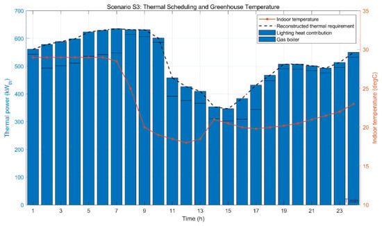
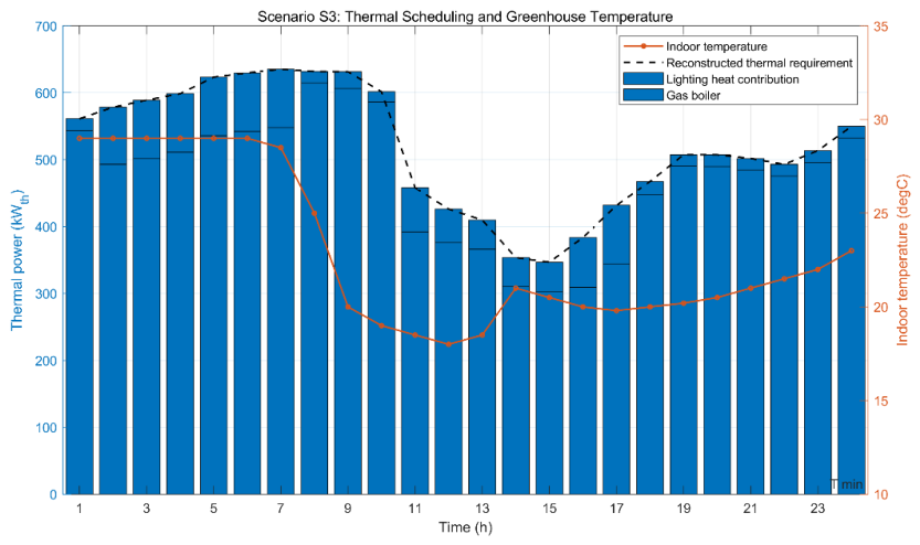
Figure 5 shows the thermal scheduling result under S3, with the corresponding thermal scheduling and greenhouse-temperature results also provided in Figure S5 in the Supplementary Materials. The total greenhouse thermal requirement is jointly satisfied by the gas boiler and the thermal contribution of supplementary lighting. The indoor greenhouse temperature varies between approximately 18 °C and 29 °C and remains well within the permitted temperature range of 10–35 °C over the entire day.

Figure 5. Thermal scheduling and greenhouse temperature under Scenario S3.

A close coupling can be observed between supplementary lighting and gas-boiler output. When the supplementary-lighting power is relatively high, the corresponding lighting heat contribution increases and part of the greenhouse thermal requirement can be supplied indirectly through lighting heat. Conversely, when lighting demand is reduced by the agricultural demand-response strategy, the gas boiler must provide a larger share of the required heat.

This behavior confirms that agricultural-load scheduling cannot be treated as an independent electrical demand-response problem. Changes in lighting power simultaneously affect electrical load, greenhouse internal heat gain, indoor temperature, and crop thermal accumulation. The coordinated scheduling framework therefore captures the interaction among the electrical, thermal, and agricultural subsystems.

The thermal-demand profile used in the scheduling extension is reconstructed from the representative-day operating conditions. Therefore, the result should be interpreted as a calibrated scheduling profile rather than a direct measurement of greenhouse heat demand.

The thermal profile is reconstructed from the validated representative-day heat demand in [4]. Envelope conduction, ground exchange, ventilation/infiltration, and solar gains are therefore represented through the calibrated net heat requirement rather than through separately identified building-physics coefficients. This choice is adequate for evaluating energy scheduling around the validated baseline but limits the model’s transferability to greenhouses with different envelope properties.

3.7. Comprehensive Performance Comparison

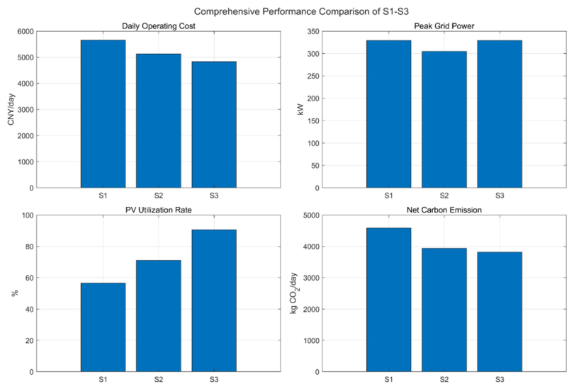
The comprehensive performance of the three scenarios is compared in Figure 6 and Table 3, with the corresponding graphical comparison and scenario comparison provided in Figure S6 and Table S2 in the Supplementary Materials, respectively. The main indicators are daily operating cost, peak-grid power, grid electricity, PV utilization, curtailed PV energy, BESS throughput, operational carbon emissions, and crop-growth indicators.

Figure 6. Comprehensive performance comparison among S1–S3: (a) daily operating cost; (b) peak-grid power; (c) PV utilization rate; and (d) operational carbon emission.

Table 3. Comparison of scheduling results under three scenarios.

Indicator	S1	S2	S3
Daily operating cost (CNY·day−1)	5657.94	5132.66	4830.43
Cost reduction relative to S1 (%)	0.00	9.28	14.63
Peak-grid power (kW)	329.25	304.91	329.25
Peak reduction relative to S1 (%)	0.00	7.39	0.00
Grid electricity (kWh·day−1)	4102.11	2826.86	2704.99
PV utilization rate (%)	56.54	71.10	90.59
Operational carbon emission (kg CO2·day−1)	4584.72	3939.31	3817.39
Lighting-regulation amount (kWh·day−1)	0.00	908.98	908.98
BESS throughput (kWh·day−1)	0.00	0.00	1362.59
DLI (mol·m−2·day−1)	16.09	12.86	12.86
GDD (°C·day)	12.96	12.96	12.96
TDRW (kg·hm−2·day−1)	225.21	180.00	180.00
Curtailed PV energy (kWh·day−1)	1597.16	1062.08	345.82

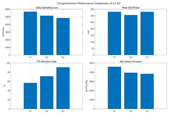
As shown in Figure 6a, the daily operating cost decreases progressively from S1 to S3. The operating costs of S1, S2, and S3 are approximately 5657.94, 5132.66, and 4830.43 CNY/day, respectively. Compared with S1, agricultural flexible-load scheduling in S2 reduces the operating cost by approximately 9.28%. After introducing coordinated BESS operation in S3, the cost reduction increases to approximately 14.63%. This demonstrates that agricultural demand flexibility and battery storage provide complementary economic benefits.

For the peak-grid power shown in Figure 6b and Figure S2 achieves the lowest value, decreasing from 329.25 kW in S1 to 304.91 kW, corresponding to a peak reduction of approximately 7.39%. This indicates that agricultural flexible-load scheduling can effectively reshape the demand profile and alleviate the maximum power drawn from the external grid. In contrast, the peak-grid power in S3 increases to 329.25 kW, which is nearly identical to that of S1. This result is mainly attributed to the current scheduling objective, which focuses on operating-cost reduction and renewable-energy utilization without explicitly penalizing the maximum-grid-import power. Therefore, the BESS in S3 is dispatched primarily for energy arbitrage and PV accommodation rather than dedicated peak shaving.

Figure 6c shows a pronounced improvement in PV utilization, defined as the ratio of utilized PV energy to total available PV energy over the 24 h horizon. The utilization rate increases from 56.54% in S1 to 71.10% in S2 and 90.59% in S3. With 3675 kWh·day⁻¹ of available PV energy, the corresponding curtailed PV energy is 1597.16, 1062.08, and 345.82 kWh·day⁻¹ for S1, S2, and S3, respectively. The improvement from S1 to S2 comes from flexible agricultural demand, while the further increase in S3 is due to BESS absorption of otherwise-curtailed solar energy.

The environmental indicator shows the same overall trend. Daily operational carbon emissions decrease from 4584.72 kg CO₂·day⁻¹ in S1 to 3939.31 kg CO₂·day⁻¹ in S2 and 3817.39 kg CO₂·day⁻¹ in S3, corresponding to a 16.74% reduction from S1 to S3. These values use the direct operational emission factors listed in Table 1 and exclude upstream/life-cycle emissions.

Unlike the other indicators, the peak-grid-power result does not decrease monotonically from S1 to S3. The peak-grid powers of S1, S2, and S3 are 329.25, 304.91, and 329.25 kW, respectively. Thus, S2 achieves a peak reduction of 7.39%, whereas S3 does not further reduce the maximum-grid demand.

This phenomenon is caused by the current scheduling objective, which prioritizes operating cost, renewable-energy utilization, and energy shifting but does not explicitly penalize the maximum-grid-import power. Consequently, the BESS in S3 is economically dispatched according to electricity prices and PV availability rather than being forced to minimize the daily peak-grid demand. This result does not indicate an infeasible BESS schedule; instead, it reveals a tradeoff between economic dispatch and explicit peak shaving. If peak-load reduction is regarded as an additional scheduling objective, a peak-demand penalty or maximum-grid-power constraint can be incorporated into the objective function.

The numerical comparison in Table 3 further confirms that the agricultural flexible load provides a substantial portion of the economic benefit even without battery participation. The transition from S1 to S2 simultaneously reduces operating cost, increases PV utilization, decreases peak-grid demand, and lowers carbon emissions. The introduction of BESS in S3 provides additional economic and renewable-energy benefits, although the current formulation does not explicitly improve peak shaving.

Overall, the results demonstrate that agricultural flexible loads and energy storage contribute through different mechanisms. Agricultural-load scheduling reshapes the temporal distribution of demand while satisfying crop-growth requirements, whereas the BESS transfers electrical energy across time and absorbs surplus renewable generation. Their coordinated operation reduces daily operating cost from 5657.94 to 4830.43 CNY/day, increases PV utilization from 56.54% to 90.59%, and decreases daily operational carbon emissions from 4584.72 to 3817.39 kg CO₂/day. These results validate the effectiveness of linking long-term equipment planning with short-term source-load-storage scheduling in rural integrated-energy systems.

3.8. Sensitivity Analysis, Comparison with Recent Literature, and Limitations

A one-at-a-time sensitivity test was performed for S3 by perturbing the TOU tariff level and available PV profile by ±20% while retaining all other parameters. Because all TOU blocks are uniformly scaled, the relative price ordering is unchanged; the dispatch pattern therefore remains the same and operating cost changes approximately proportionally. PV availability has a stronger operational effect: a 20% reduction raises peak-grid import by about 40.7% and operational carbon emissions by about 5.6%, whereas a 20% increase lowers carbon emissions by about 2.5% but also reduces the utilization ratio because more solar energy becomes available than the load/BESS can absorb. The detailed sensitivity results are summarized in Table 4.These results confirm that the value of the coordinated schedule depends more strongly on renewable availability than on a uniform rescaling of the tariff.

Table 4. Local sensitivity of S3 to TOU tariff and PV-availability perturbations.

Perturbation	Operating-Cost Change (%)	Peak-Grid Change (%)	PV Utilization (%)	Carbon Change (%)
TOU tariff −20%	−3.02	0.00	90.59	0.00
TOU tariff +20%	+3.02	0.00	90.59	0.00
PV availability −20%	+2.89	+40.72	100.00	+5.60
PV availability +20%	−1.28	−0.61	79.40	−2.47

Table 4. Local sensitivity of S3 to TOU tariff and PV-availability perturbations.

Perturbation	Operating-Cost Change (%)	Peak-Grid Change (%)	PV Utilization (%)	Carbon Change (%)
TOU tariff −20%	−3.02	0.00	90.59	0.00
TOU tariff +20%	+3.02	0.00	90.59	0.00
PV availability −20%	+2.89	+40.72	100.00	+5.60
PV availability +20%	−1.28	−0.61	79.40	−2.47

The planning-side sensitivity to endogenous PV expansion is not evaluated because PV is a pre-existing sunk asset in the studied village. Likewise, a full re-optimization of capacity under battery-capital-cost uncertainty would require repeating the annual bilevel planning study. To keep the revision transparent, we do not infer uncomputed capacity changes; instead, this limitation is stated explicitly and identified as a priority for future work.

The present findings are consistent with, but not directly numerically comparable to, recent studies because system boundaries and objectives differ. Lin et al. [13] reported 6.98% cost reduction from greenhouse operational optimization and 43.50% reduction in total cost under a different hierarchical PV–battery objective. Kushwaha et al. [19] reported a 13.10% reduction in cost of energy and 28.13% reduction in carbon emissions for a rural autonomous distributed-generation system using load scheduling. Ajagekar et al. [16] demonstrated demand-response benefits for networked PV–battery greenhouses using multi-agent reinforcement learning, while Mohebi and Roshandel [18] showed that joint design-operation optimization of greenhouse heating can reduce CO₂ emissions by 22.4%. In contrast, the present study reports a 9.01% planning-cost reduction and a 14.63% day-ahead operating-cost reduction while explicitly enforcing cumulative crop-growth constraints and passing planned capacities into the scheduling stage.

The evaluation therefore spans technical indicators (peak-grid power, PV utilization, curtailment, BESS throughput), economic indicators (annual planning cost and daily operating cost), environmental indicators (direct operational CO₂ emissions), and an agronomic/social-acceptability proxy (maintenance of prescribed crop-growth constraints without involuntary load shedding). A full social assessment—such as employment, farmer acceptance, comfort preference, or distributional impacts—is not quantified because no field survey or socioeconomic dataset is available for the case study.

The principal limitations are: (i) the day-ahead demonstration uses one pepper representative day and deterministic forecasts; different crop stages and weather conditions can change the operating value of PV, BESS, and lighting flexibility; (ii) κ_PAR, lighting heat gain, and thermal inertia are calibrated aggregate surrogates rather than fixture- and greenhouse-specific identified parameters; (iii) PAR, DLI, GDD, temperature, and TDRW are physiological proxies and cannot guarantee realized yield under pests, nutrients, CO₂, humidity, and other agronomic factors; (iv) the BESS degradation model is linear; (v) upstream/life-cycle emissions and broader social indicators are excluded; and (vi) probabilistic reliability indices such as LOLE, EENS, SAIDI, and SAIFI are not computed because outage states are not modeled. Hourly power balance enforces zero deterministic unserved energy in all feasible scenarios, but a dedicated reliability study requires component-outage and uncertainty models.

4. Conclusions

This study establishes a crop-growth-constrained planning–scheduling framework for a rural integrated-energy system. The main conclusions are:

(1) The crop-growth-stage planning method changes the capacity mix toward greater storage flexibility and reduces total annual planning cost from 23.08 × 10⁵ to 21.00 × 10⁵ CNY (9.01%). The cost decomposition shows that the main benefit comes from lower annual operating cost rather than lower investment expenditure.

(2) Under the planned capacities, flexible agricultural-load regulation alone reduces day-ahead operating cost by 9.28%. Coordinating the same agricultural flexibility with BESS operation increases the reduction to 14.63%, raises PV utilization from 56.54% to 90.59%, lowers curtailed PV energy to 345.82 kWh·day⁻¹, and reduces direct operational carbon emissions by 16.74%. S3 does not further reduce peak-grid power because peak demand is not included in the economic objective.

(3) The case demonstrates that crop-growth constraints can bound economic flexibility, but the results should not be interpreted as a direct yield guarantee or as evidence of robustness across all seasons. Future work will extend the scheduling study to multiple crop stages and stochastic weather, introduce nonlinear BESS aging and explicit peak/carbon objectives, identify greenhouse-specific PAR/thermal parameters, and add probabilistic reliability and socioeconomic assessments.

References

- Gorjian, S.; Calise, F.; Kant, K.; Ahamed, M.S.; Copertaro, B.; Najafi, G.; Zhang, X.; Aghaei, M.; Shamshiri, R.R. A review on opportunities for implementation of solar energy technologies in agricultural greenhouses. J. Clean. Prod. 2021, 285, 124807. [Google Scholar] [CrossRef] [Scilit]
- Hassanien, R.H.E.; Li, M.; Wang, Y.; Hadibi, T.; Kumar, A.; Song, M. Review on photovoltaic greenhouses for sustainable food and energy production. Sol. Energy 2025, 302, 114030. [Google Scholar] [CrossRef] [Scilit]
- Zhao, Y.; Luo, H.; Liu, C.; Qiu, J.; Li, X.; Han, L.; Chen, Y.; Jiang, Y. Photovoltaic greenhouses as integrated agro-energy systems: Spectral regulation, crop-energy coordination, and unified assessment—A review. Renew. Sustain. Energy Rev. 2026, 235, 116933. [Google Scholar] [CrossRef] [Scilit]
- Fu, X.; Wei, Z.; Sun, H.; Zhang, Y. Agri-energy-environment synergy-based distributed energy planning in rural areas. IEEE Trans. Smart Grid 2024, 15, 3722–3738. [Google Scholar] [CrossRef] [Scilit]
- Kamal, M.M.; Asharaf, I.; Fernandez, E. Optimal renewable integrated rural energy planning for sustainable energy development. Sustain. Energy Technol. Assess. 2022, 53, 102581. [Google Scholar] [CrossRef] [Scilit]
- Du, Y.; Xue, Y.; Lu, L.; Yu, C.; Zhang, J. A bi-level co-expansion planning of integrated electric and heating system considering demand response. Front. Energy Res. 2022, 10, 999948. [Google Scholar] [CrossRef] [Scilit]
- Du, Y.; Xue, Y.; Wu, W.; Shahidehpour, M.; Shen, X.; Wang, B.; Sun, H. Coordinated Planning of Integrated Electric and Heating System Considering the Optimal Reconfiguration of District Heating Network. IEEE Trans. Power Syst. 2024, 39, 794–808. [Google Scholar] [CrossRef] [Scilit]
- Zhang, J.; Chang, X.; Wu, D.; Xue, Y.; Su, J.; Sun, H. Optimal location and capacity planning of distribution network considering demand response and battery storage capacity degradation. In Proceedings of the 2023 IEEE 7th Conference on Energy Internet and Energy System Integration (EI2), Hangzhou, China, 15 – 18 December 2023. [Google Scholar]
- Ding, B.; Li, Z.; Li, Z.; Xue, Y.; Chang, X.; Su, J.; Jin, X.; Sun, H. A CCP-based distributed cooperative operation strategy for multi-agent energy systems integrated with wind, solar, and buildings. Appl. Energy 2024, 365, 123275. [Google Scholar] [CrossRef] [Scilit]
- Wang, K.; Xue, Y.; Zhou, Y.; Li, Z.; Chang, X.; Sun, H. Distributed coordinated reconfiguration with soft open points for resilience-oriented restoration in integrated electric and heating systems. Appl. Energy 2024, 365, 123207. [Google Scholar] [CrossRef] [Scilit]
- Fu, X.; Zhou, Y. Collaborative optimization of PV greenhouses and clean energy systems in rural areas. IEEE Trans. Sustain. Energy 2023, 14, 642–656. [Google Scholar] [CrossRef] [Scilit]
- Tan, H.; Li, Z.; Wang, Q.; Mohamed, M.A. A novel forecast scenario-based robust energy management method for integrated rural energy systems with greenhouses. Appl. Energy 2023, 330, 120343. [Google Scholar] [CrossRef] [Scilit]
- Lin, D.; Dong, Y.; Ren, Z.; Zhang, L.; Fan, Y. Hierarchical optimization for the energy management of a greenhouse integrated with grid-tied photovoltaic–battery systems. Appl. Energy 2024, 374, 124006. [Google Scholar] [CrossRef] [Scilit]
- Mosharafian, S.; Afzali, S.; Weaver, G.M.; van Iersel, M.W.; Mohammadpour Velni, J. Optimal lighting control in greenhouse by incorporating sunlight prediction. Comput. Electron. Agric. 2021, 188, 106300. [Google Scholar] [CrossRef] [Scilit]
- Li, P.; Zhao, M.; Zhang, H.; Zhang, O.; Li, N.; Yue, X.; Tan, Z. An operational optimization model for micro energy grids in photovoltaic-storage agricultural greenhouses based on operation mode selection. Processes 2025, 13, 1622. [Google Scholar] [CrossRef] [Scilit]
- Ajagekar, A.; Decardi-Nelson, B.; You, F. Energy management for demand response in networked greenhouses with multi-agent deep reinforcement learning. Appl. Energy 2024, 355, 122349. [Google Scholar] [CrossRef] [Scilit]
- Sipos, L.; Boros, I.F.; Csambalik, L.; Székely, G.; Jung, A.; Balázs, L. Horticultural lighting system optimalization: A review. Sci. Hortic. 2020, 273, 109631. [Google Scholar] [CrossRef] [Scilit]
- Mohebi, P.; Roshandel, R. Optimal design and operation of solar energy system with heat storage for agricultural greenhouse heating. Energy Convers. Manag. X 2023, 18, 100353. [Google Scholar] [CrossRef] [Scilit]
- Kushwaha, P.K.; Bhattacharjee, C.; Maurya, A.K. Techno-economic-enviro-socio analysis of autonomous unified distributed generation using load scheduling approach and dispatch strategies. Electr. Eng. 2025, 107, 15133–15159. [Google Scholar] [CrossRef] [Scilit]
- Seginer, I.; Albright, L.D.; Ioslovich, I. Improved strategy for a constant daily light integral in greenhouses. Biosyst. Eng. 2006, 93, 69–80. [Google Scholar] [CrossRef] [Scilit]
- Bhuiyan, R.; van Iersel, M.W. Only extreme fluctuations in light levels reduce lettuce growth under sole source lighting. Front. Plant Sci. 2021, 12, 619973. [Google Scholar] [CrossRef] [Scilit]
- van Henten, E.J. Validation of a dynamic lettuce growth model for greenhouse climate control. Agric. Syst. 1994, 45, 55–72. [Google Scholar] [CrossRef] [Scilit]
- Albright, L.D.; Both, A.J.; Chiu, A.J. Controlling greenhouse light to a consistent daily integral. Trans. ASAE 2000, 43, 421–431. [Google Scholar] [CrossRef] [Scilit]
- Yang, R.; Qiu, C.; Zheng, J.; Ji, F.; He, D.; Yang, P. LED supplementary strategy based on hourly light integral for improving the yield and quality of greenhouse strawberries. Int. J. Agric. Biol. Eng. 2024, 17, 96–104. [Google Scholar] [CrossRef] [Scilit]
- Jayalath, T.C.; van Iersel, M.W.; Ferrarezi, R.S. The energy requirement for supplemental greenhouse lighting can be reduced by considering ‘excess’ light from the previous day. Plants 2024, 13, 652. [Google Scholar] [CrossRef] [Scilit]
- Wang, Y.; Su, J.; Xue, Y.; Chang, X.; Li, Z.; Sun, H. Toward rolling optimal dispatch strategy considering alert mechanism for Antarctic electricity-hydrogen-heat integrated energy system. IEEE Trans. Sustain. Energy 2024, 15, 2457–2471. [Google Scholar] [CrossRef] [Scilit]
- Hu, H.; Ma, Y.; Zhang, X.; Han, C.; Hao, Y. Day-ahead and hour-ahead optimal scheduling for battery storage of renewable energy power stations participating in primary frequency regulation. Front. Energy Res. 2024, 12, 1424389. [Google Scholar] [CrossRef] [Scilit]
- Clausen, A.; Mærsk-Møller, H.M.; Sørensen, J.C.; Jørgensen, B.N.; Kjær, K.H.; Ottosen, C.O. Integrating commercial greenhouses in the smart grid with demand response based control of supplemental lighting. In Proceedings of the 2015 International Conference on Industrial Technology and Management Science; Atlantis Press: Paris, France, 2015; pp. 199–213. [Google Scholar]
- Maeda, K.; Masuda, E.; Tamashiro, T.; Maharjan, G.; Maruo, T. Comparison of supplemental LED top- and interlighting for year-round production of cherry tomato. Agronomy 2022, 12, 1878. [Google Scholar] [CrossRef] [Scilit]
- Lee, J.-O.; Kim, Y.-S. Novel battery degradation cost formulation for optimal scheduling of battery energy storage systems. Int. J. Electr. Power Energy Syst. 2022, 137, 107795. [Google Scholar] [CrossRef] [Scilit]
- Zhou, B.; Liu, X.; Cao, Y.; Li, C.; Chung, C.Y.; Chan, K.W. Optimal scheduling of virtual power plant with battery degradation cost. IET Gener. Transm. Distrib. 2016, 10, 712–725. [Google Scholar] [CrossRef] [Scilit]
- Fu, X.; Bai, J.; Sun, H.; Zhang, Y. Optimizing agro-energy-environment synergy in agricultural microgrids through carbon accounting. IEEE Trans. Smart Grid 2024, 15, 4819–4834. [Google Scholar] [CrossRef] [Scilit]
- Cui, Z.; Chang, X.; Xue, Y.; Yi, Z.; Li, Z.; Sun, H. Distributed peer-to-peer electricity-heat-carbon trading for multi-energy virtual power plants considering Copula-CVaR theory and trading preference. Int. J. Electr. Power Energy Syst. 2024, 162, 110231. [Google Scholar] [CrossRef] [Scilit]
- Wu, D.; Chang, X.; Xue, Y.; Huang, Y.; Su, J.; Sun, H. Bilevel low-carbon coordinated operation of integrated energy systems considering dynamic tiered carbon pricing methodology. Energy 2024, 310, 133251. [Google Scholar] [CrossRef] [Scilit]
Disclaimer/Publisher’s Note: The statements, opinions and data contained in all publications are solely those of the individual author(s) and contributor(s) and not of MDPI and/or the editor(s). MDPI and/or the editor(s) disclaim responsibility for any injury to people or property resulting from any ideas, methods, instructions or products referred to in the content. |
© 2026 by the authors. Licensee MDPI, Basel, Switzerland. This article is an open access article distributed under the terms and conditions of the Creative Commons Attribution (CC BY) license.