Small-Signal Stability of Photovoltaic Systems Connected to Weak Grids Based on Linear Time-Periodic Theory: Phase-Locked Loop Analysis and Virtual Inductance Control

Abstract

Large-scale photovoltaic (PV) plants connected to weak grids may experience oscillations caused by interactions between converter controls and grid impedance. This paper develops a linear time-periodic (LTP) small-signal model by linearizing nonlinear electromagnetic-transient (EMT) equations along the periodic steady-state trajectory, explicitly incorporating second-order generalized integrator (SOGI)-based positive-/negative-sequence separation and negative-sequence current control. Model accuracy is validated through time-domain response comparisons with the nonlinear model under DC-link voltage reference, grid frequency, and grid voltage disturbances. Floquet characteristic exponent trajectories reveal critical-mode migration as the phase-locked loop (PLL) proportional and integral gains vary. Three-dimensional stability surfaces and their projections characterize changes in the PLL proportional–integral (PI) parameter stability region as the short-circuit ratio (SCR) decreases from 2.63 to 1.47. Participation factor analysis identifies PLL states as the dominant contributors to the critical oscillatory modes. Accordingly, virtual inductance control is adopted to construct a virtual point of common coupling (PCC) voltage for PLL synchronization. Under the weak grid condition with SCR = 1.47, the range of the virtual inductance control coefficient that maintains small-signal stability extends from just above approximately 0.25 to 1. With a representative coefficient of 0.4, nonlinear EMT simulations and parameter scans demonstrate that the control suppresses oscillations and enlarges the PLL PI parameter stability region.

1. Introduction

Large-scale photovoltaic (PV) power plants are commonly installed in remote regions and connected to the main grid through long alternating-current (AC) transmission corridors. The resulting short-circuit ratio (SCR) at the point of common coupling (PCC) can be low, and the interaction between converter controls and grid impedance becomes pronounced. Small-signal modeling has been used to investigate the factors affecting the stability of PV generation connected to weak AC grids [1]. Models of voltage-source converters under weak grid conditions have further revealed the dynamic interactions between the grid and direct-current (DC) link voltage control [2]. Harmonic stability studies have examined converter–network interactions and the associated modeling methods from a broader power electronics-based power system perspective [3]. Recent research on the synchronization stability of grid-connected inverters has analyzed the effects of phase-locked loop (PLL) and grid parameters on transient synchronization and introduced a feedback low-pass filter into the PLL to improve stability [4].

The operating performance of PV systems also depends on their connection locations and network configuration. Research on the optimal placement of PV systems and electric vehicle charging stations, considering area and location constraints, has shown that equipment locations affect distribution network losses and voltage performance [5]. Alongside these network-level considerations, the internal control dynamics of converters require attention. The angle estimated by the PLL enters the voltage and current coordinate transformations, making PLL parameters important to the dynamic coupling between the converter and the grid. Modal resonance between the PLL and DC-link voltage control has been identified under weak grid conditions, demonstrating that interactions between control loops can reduce system damping [6]. Weak grid stability assessment therefore requires consideration of both grid conditions and internal converter control dynamics.

Small-signal analysis is central to controller design and grid connection stability assessment. A review of small-signal modeling for AC power electronic systems has compared different approaches and established a unified modeling framework [7]. Under unbalanced grid conditions, complex-valued multifrequency admittance models can represent the frequency-coupling characteristics of three-phase converters [8]. The equivalence between modified sequence-domain and dq-domain impedance definitions provides a link between impedance-based stability analyses in different reference frames [9]. For stability enhancement, compensation of the impedance voltage drop in the synchronization signal can extend the stable operating range of voltage-source converters connected to weak grids [10]. Impedance-based methods are useful for terminal-level stability assessment, while state-space and modal analyses provide further insight into the associations between specific oscillatory modes and internal control states.

The dynamics of synchronization and sequence separation are also relevant to model development. A review of three-phase PLLs has examined different synchronization structures and their dynamic characteristics, providing a basis for PLL selection and parameter design [11]. Passivity-based analysis accounting for sequence decomposition algorithms has further shown that sequence separation dynamics affect converter harmonic stability and should be represented in the corresponding models [12]. A recent state-space model of grid-following voltage-source converters has used eigenvalue analysis to determine the maximum stable power transfer under different grid strengths and resistance-to-reactance ratios, demonstrating the dependence of stability boundaries on grid conditions [13]. When positive- and negative-sequence components and their interactions are considered, the model must also retain the periodic characteristics introduced by sequence separation and coordinate transformations.

Dynamic-phasor methods describe system dynamics using time-varying Fourier coefficients and have been applied to LCC-HVDC modeling [14]. Generalized dynamic-phasor models have also been developed for small-signal stability analysis of modular multilevel converters [15]. Harmonic state-space (HSS) methods use harmonic expansion to represent coupling between different frequency components and have been applied to harmonic interaction analysis in grid-connected converters [16]. However, numerical implementation of HSS models requires finite-order truncation. Studies of truncation order selection based on Floquet characteristic exponents show that model accuracy and computational effort must both be considered [17].

Linear time-periodic (LTP) theory provides an alternative framework for retaining system periodicity. LTP-based eigenvalue analysis and harmonic impedance estimation have been used to assess the stability of power converter-based AC systems [18]. LTP modeling of voltage-source converters has further demonstrated the application of this framework to converter stability analysis [19]. For grid-connected inverters with proportional resonant control, Floquet-based time-domain methods can assess the stability of periodic operation [20]. Floquet–Lyapunov theory also provides a theoretical basis for the analysis and control of linear time-periodic systems [21]. More recently, eigenstructure-preserved LTP theory has established participation factor and sensitivity formulations to quantify the associations between electromagnetic modes, system states, and parameters [22]. HSS eigenvalue sensitivity analysis for nonlinear time-periodic systems provides an additional means of examining how parameter variations affect stability [23].

On the PV side, maximum power-point tracking (MPPT) control can also influence system dynamics. Comparisons under fast-changing irradiance have shown that deep reinforcement learning and conventional MPPT strategies exhibit different performance in power extraction, DC-link voltage regulation, and transient response [24]. Model development for a specific stability problem therefore requires a clear definition of the dynamics of interest and the corresponding modeling scope. This study focuses on converter–grid electromagnetic dynamics under specified PV-side operating conditions, with the PV-side modeling assumptions described in Section 2.1.

These studies provide a foundation for weak grid stability analysis and control design. For grid-connected PV systems incorporating SOGI-based positive-/negative-sequence separation and negative-sequence current control, further analysis within a unified LTP framework is needed to examine the relationships among PLL parameters, grid strength, and stability enhancement control. Accordingly, this paper combines model validation, modal identification, and control effectiveness assessment within the same LTP framework. The main contributions are as follows:

(1)

An LTP small-signal model of a grid-connected PV system is developed, explicitly accounting for SOGI-based positive-/negative-sequence separation and negative-sequence current control while retaining the inherent periodic dynamics of the system. Time-domain response waveforms obtained from the LTP model are compared with those from the nonlinear electromagnetic-transient (EMT) model under three disturbance scenarios. Root-mean-square error and maximum absolute error are used to quantify the numerical deviations between the two models, thereby validating the accuracy of the developed model.

(2)

Floquet characteristic exponent trajectories are used to analyze the effects of the PLL proportional and integral gains on system stability at an SCR of 2.63. The PLL proportional–integral (PI) parameter stability boundaries are then used to examine the influence of grid strength on the stable parameter region as the SCR decreases from 2.63 to 1.47. Participation factor analysis establishes the associations between system modes and states. Under the very weak grid condition with an SCR of 1.47, the participation factor magnitudes of the PLL PI integrator state and angle state for the critical oscillatory mode pair are approximately 0.3995 and 0.4330, respectively. These values are markedly higher than those of the other states, identifying the PLL dynamics as the dominant contributors to the critical oscillatory mode.

(3)

Based on the participation factor analysis, virtual inductance control is adopted to construct a virtual PCC voltage for PLL synchronization and improve the damping of the PLL-dominated oscillatory mode. The characteristic exponent trajectories indicate that, under the investigated very weak grid condition, the control coefficient range that restores small-signal stability extends from just above approximately 0.25 to 1. A coefficient of 0.4, located within the identified stable interval with a margin from the critical boundary, is selected for subsequent validation. Nonlinear EMT time-domain simulations and comparisons of the PLL parameter stability regions verify, respectively, the oscillation suppression effect of control and its ability to enlarge the stable parameter region.

2. LTP Modeling of the Grid-Connected PV System

2.1. System Topology and Control Architecture

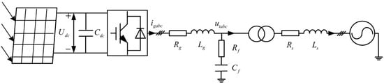
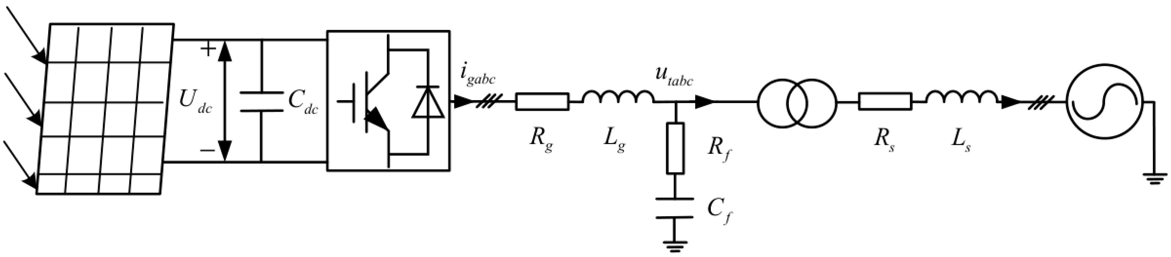
The PV system under study consists of a controlled direct-current source, DC-link capacitor, voltage-source converter (VSC), inductor–capacitor (LC) filter, transformer, grid line, and infinite bus, as shown in Figure 1.

Figure 1. Topology of grid-connected PV system.

Following the multi-time-scale modeling perspective discussed in [25], this study focuses on the converter–grid electromagnetic dynamics and their coupling with the PLL, voltage wcontrol, and current control loops. Under constant irradiance and temperature, the MPPT reference is assumed to remain unchanged over the disturbance interval, and MPPT dynamics are therefore not explicitly modeled. An average-value converter model is adopted, with the PV array represented by an ideal controlled current source while retaining the dynamics of the DC-link capacitor. This approximation retains the converter and grid electromagnetic dynamics while reducing the model order.

In Figure 1, C_dc and U_dc denote the DC-link capacitance and voltage; i_gabc is the VSC output current; L_g and R_g are the filter inductance and its series resistance; C_f and R_f are the filter capacitance and series resistance; L_s and R_s are the grid-line inductance and resistance; and u_tabc is the PCC voltage. The main electrical and control parameters are listed in Table A1 in Appendix A.

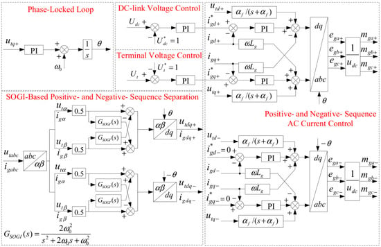
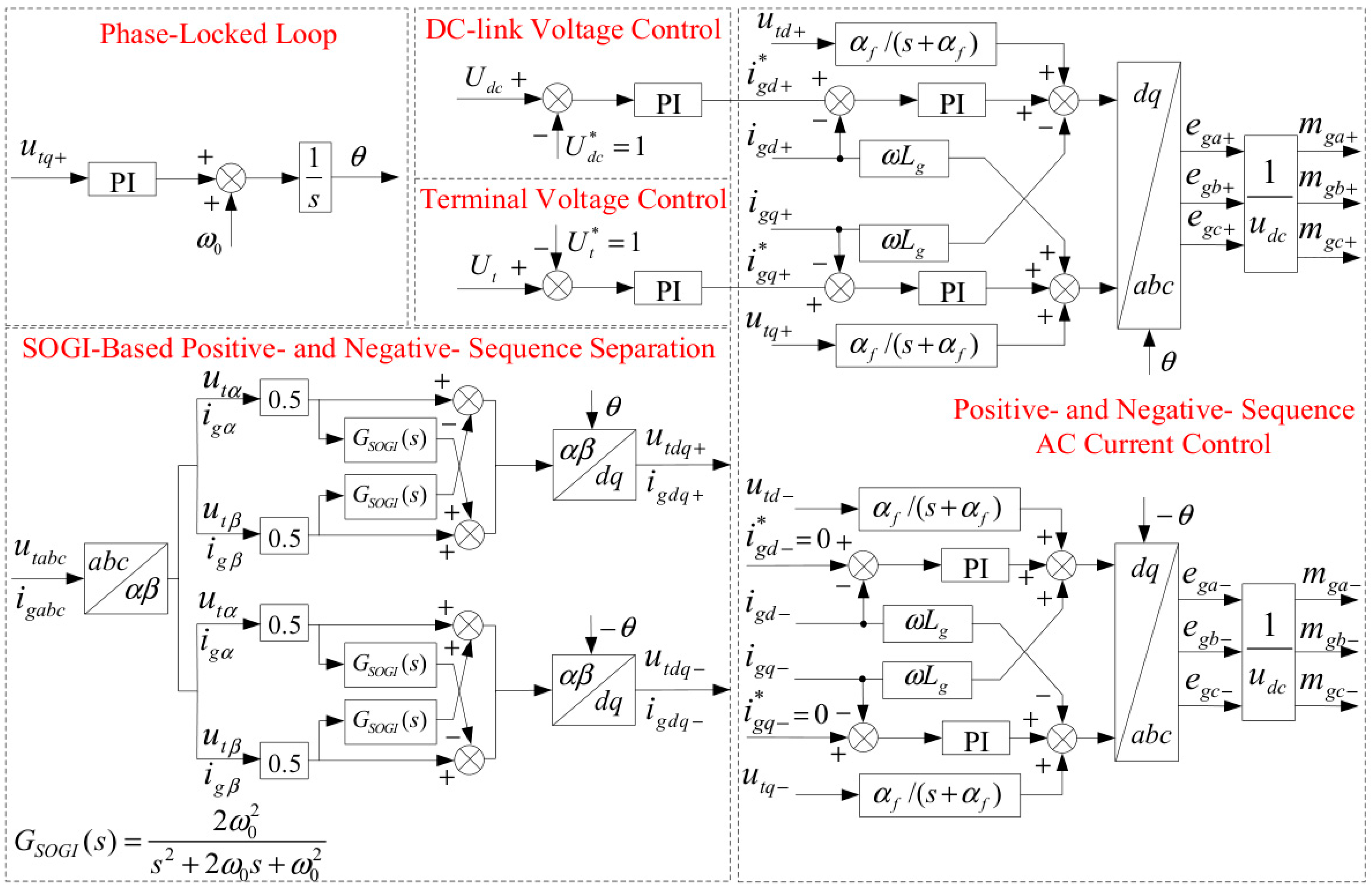
The VSC employs a second-order generalized integrator (SOGI) for positive-/negative-sequence separation. The control architecture also contains the phase-locked loop (PLL), DC-link voltage control (DVC), terminal voltage control (TVC), and positive-/negative-sequence AC current control (ACC), as shown in Figure 2. Positive-/negative-sequence decoupling and coordinate transformations dependent on the PLL angle make the linearized system matrix periodic and time-varying.

Figure 2. Control architecture of grid-connected PV converter.

2.2. Mathematical Relations of Sequence Separation and PLL

The sequence decomposition algorithm (SDA) extracts the positive-/negative-sequence components by combining each stationary-frame αβ signal with its quadrature signal. Following [12], the quadrature operator provides a 90° phase lag at the fundamental frequency. In this paper, this operator is implemented using the second-order generalized integrator G_SOGI(s) shown in Figure 2. For z ∈ {u_t, i_g}, the second-integrator state x₂ is defined as one half of the complete quadrature signal, thereby incorporating the 0.5 weighting of the quadrature terms in the sequence separation branches. The corresponding SOGI state equations are given by the following:

$${\dot{x}}_1={\omega }_0({\omega }_0{z}_{\alpha \beta }-{\omega }_0{x}_2-2x_1);$$

(1)

$${\dot{x}}_2=x_1,$$

(2)

where ω₀ is the nominal grid angular frequency, z_αβ is the stationary-frame voltage or current vector, and x₁ and x₂ are the corresponding first- and second-integrator state vectors. Accordingly, the complete quadrature signal used for sequence separation is recovered as z_αβ⊥ = 2x₂, and the transfer function from z_αβ to z_αβ⊥ is given by the following:

$$G_{SOGI}(s)={\displaystyle \frac{2{\omega }_0^2}{s^2+2{\omega }_{0}s+{\omega }_0^2}},$$

(3)

At s = jω₀, (3) has unit magnitude and a −90° phase shift. Thus, G_SOGI(s) produces the quadrature signal required by the cross-coupling branches in Figure 2. The positive- and negative-sequence components are then given by the following:

z_α+ = 0.5(z_α − z_β⊥);

(4)

z_β+ = 0.5(z_α⊥ + z_β);

(5)

z_α− = 0.5(z_α + z_β⊥);

(6)

z_β− = 0.5(−z_α⊥ + z_β),

(7)

where z denotes either the terminal voltage quantity u_t or the converter output current i_g; the subscripts + and − denote the positive- and negative-sequence components, respectively; and z_α⊥ and z_β⊥ are the outputs of G_SOGI(s) for the α- and β-axis inputs. The opposite signs in the cross-coupling terms distinguish the two sequences. Applying the same operation to u_tαβ and i_gαβ gives the separated voltage and current components. Their relations between the stationary and rotating frames are expressed as follows:

z_αβ = T_Cz_abc;

(8)

z_dq± = P_±θz_αβ±;

(9)

$$T_C={\displaystyle \frac{2}{3}}\left[\begin{array}{ccc}1& -{\displaystyle \frac{1}{2}}& -{\displaystyle \frac{1}{2}}\\ 0& {\displaystyle \frac{\sqrt{3}}{2}}& -{\displaystyle \frac{\sqrt{3}}{2}}\end{array}\right];$$

(10)

$$P_{\pm \theta }=\left[\begin{array}{cc}\cos (\pm \theta )& \sin (\pm \theta )\\ -\sin (\pm \theta )& \cos (\pm \theta )\end{array}\right].$$

(11)

where T_C is the amplitude-invariant Clarke matrix and P_+θ and P_−θ denote the Park matrices for the positive-/negative-sequence transformations, respectively. The positive-sequence q-axis PCC voltage u_tq+ drives the synchronous reference-frame PLL. By introducing the PLL integrator state x_ω, the PLL dynamics are expressed as follows [10,11]:

$${\dot{x}}_{\omega }=k_{ipll}{u}_{tq+};$$

(12)

ω_s = k_ppllu_tq+ + x_ω;

(13)

$$\dot{\theta }={\omega }_s+{\omega }_0.$$

(14)

where k_ppll and k_ipll are the PLL proportional and integral gains, respectively; x_ω is the integrator state of the PI controller; ω_s is the frequency correction produced by the PI controller; and θ is the estimated grid angle. The DVC, TVC, and ACC are represented by their PI integrator states together with voltage feedforward and current decoupling terms. Linearizing these controller equations, the SOGI relations, and the electrical network along the same periodic steady-state trajectory yields the LTP state-space model used in the subsequent analysis.

2.3. Trajectory Linearization and Floquet Stability Criterion

Let the electrical network states, SOGI states, controller integrator outputs, and filter states be collected in x, and let x₀(t) denote the periodic steady-state solution obtained from the nonlinear EMT model. Following the trajectory linearization framework in [18,19,20], the nonlinear vector field is expanded to the first order at each point along x₀(t). Defining the perturbation as Δx(t) = x(t) − x₀(t), the resulting first-order perturbation dynamics are expressed as follows:

$$\Delta \dot{\mathit{x}}=\mathit{A}(t)\Delta \mathit{x}(t)$$

(15)

where the periodic state matrix is defined as follows:

$$\mathit{A}(t)=\partial f/\partial x{|}_{x_0(t)}=\mathit{A}(t+T)$$

(16)

Here, A(t) is the Jacobian evaluated along x₀(t), A(t + T) = A(t), and T is the fundamental period. The periodicity of A(t) is mainly introduced by the angle-dependent sequence transformations. The resulting state vector contains the electrical network, controller, SOGI, and filter states.

Unlike harmonic expansion, trajectory linearization retains the periodic coefficients directly and does not introduce a truncation order. Let Φ(t,0) denote the state transition matrix initialized by Φ(0,0) = I. Integration over one fundamental period produces the monodromy matrix Φ(T,0); its eigenvalues μ_i are the Floquet characteristic multipliers, and the corresponding characteristic exponents λ_i are given by the following:

μ_i = eig[Φ(T,0)]

(17)

λ_i = ln(μ_i)/T

(18)

Let us define the stability metric η = max[Re(λ_i)]. The periodic solution is asymptotically stable when η < 0, critical when η = 0, and unstable when η > 0 [18,19,21]. The real part of each characteristic exponent measures modal damping. The frequency corresponding to its imaginary part does not directly represent the actual modal oscillation frequency; the two generally differ by an integer multiple of the fundamental frequency.

2.4. Model Validation

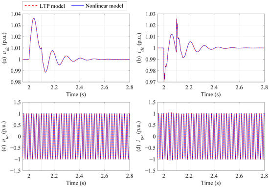
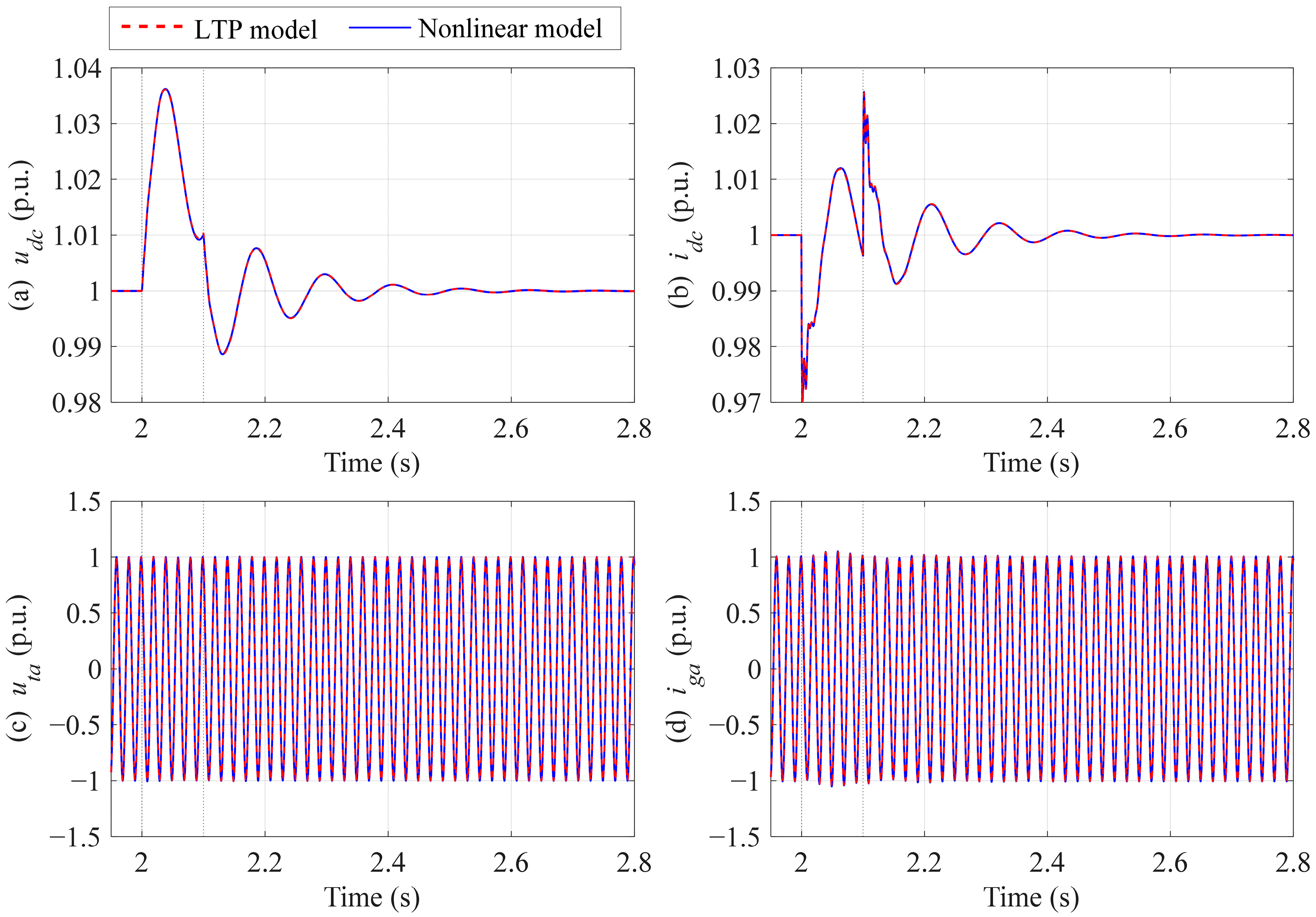
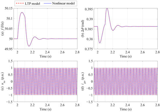
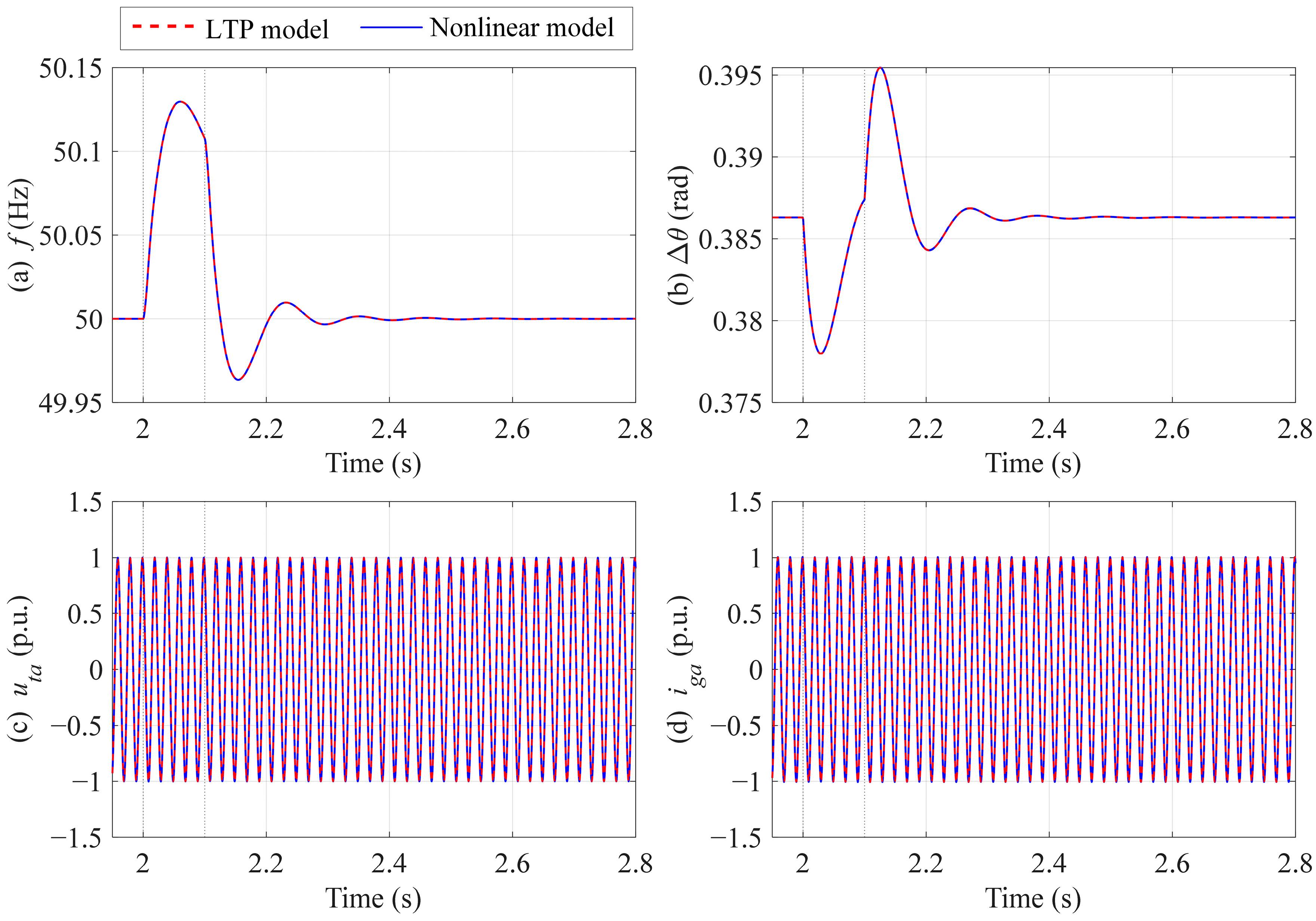
The nonlinear EMT model and its LTP linearization are simulated separately in MATLAB R2024b. To validate the accuracy of the proposed LTP model, three disturbance scenarios are considered: a DC-link voltage reference perturbation, a grid frequency perturbation, and a balanced three-phase voltage sag. In all scenarios, the line inductance is L_s = 0.2 p.u., and the short-circuit ratio, including the line and transformer impedances, is SCR = 2.63. The proportional and integral gains of the PLL are 50 and 2000, respectively. Each disturbance is applied at t = 2 s and removed at t = 2.1 s, while the remaining controller parameters and network settings are held constant. Figure 3, Figure 4 and Figure 5 compare the time-domain responses of the two models over 1.95–2.8 s.

Figure 3. Time-domain response comparison between the LTP and nonlinear EMT models under a DC-link voltage reference perturbation. (a) The DC-link voltage u_dc. (b) The DC-link current i_dc. (c) The phase-A PCC voltage u_ta. (d) The phase-A converter current i_ga.

Figure 4. Time-domain response comparison between the LTP and nonlinear EMT models under a grid frequency perturbation. (a) The PLL frequency f. (b) The PLL angle relative to the grid-source angle Δθ. (c) The phase-A PCC voltage u_ta. (d) The phase-A converter current i_ga.

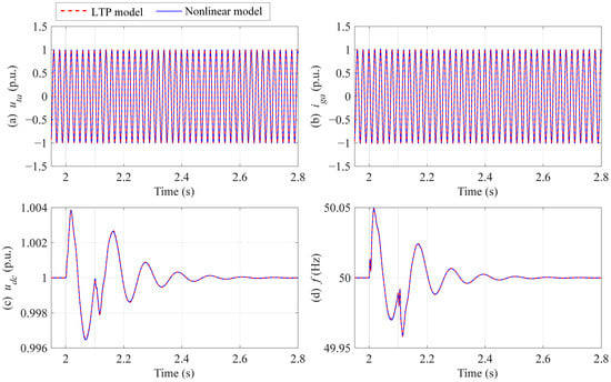
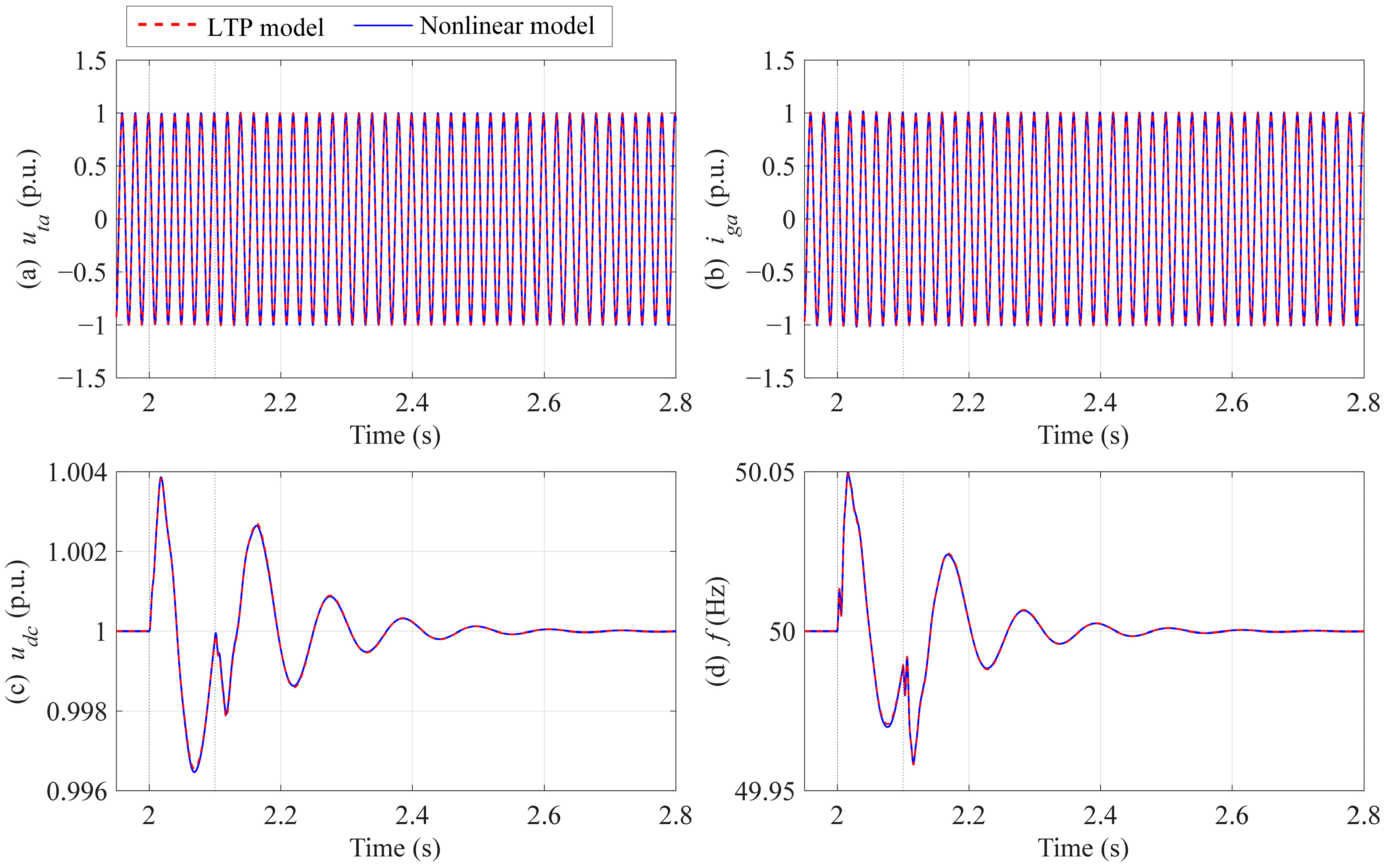
Figure 5. Time-domain response comparison between the LTP and nonlinear EMT models under a balanced three-phase voltage sag. (a) The phase-A PCC voltage u_ta. (b) The phase-A converter current i_ga. (c) The DC-link voltage u_dc. (d) The PLL frequency f.

Disturbance scenario 1: DC-link voltage reference perturbation. Initially, the system operates with a DC-link voltage reference of 1.0 p.u. At t = 2 s, the reference is increased to 1.02 p.u. and then restored to 1.0 p.u. at t = 2.1 s. Figure 3 compares the DC-link voltage u_dc, the DC-link current i_dc, the phase-A PCC voltage u_ta, and the phase-A converter current i_ga. The two models show close agreement in their transient oscillations, damping behavior, and recovery following both the application and removal of the disturbance. These results demonstrate that the LTP model accurately captures the DC-link voltage control dynamics and their coupling with the AC-side response.

Disturbance scenario 2: Grid frequency perturbation. At t = 2 s, the grid frequency is increased from 50 Hz to 50.1 Hz and then restored to 50 Hz at t = 2.1 s. The grid-source phase remains continuous throughout the process. Figure 4 compares the PLL frequency f, the PLL angle relative to the grid source Δθ, the phase-A PCC voltage u_ta, and the phase-A converter current i_ga. Here, θ_PLL denotes the PLL output angle, and θ_grid denotes the phase angle of the grid-source voltage. The frequency and relative angle are defined as f = (1/2π) dθ_PLL/dt and Δθ = θ_PLL − θ_grid, respectively. The two models show close agreement in the PLL frequency, relative angle, and AC electrical responses during the frequency perturbation and subsequent recovery. These results validate the ability of the LTP model to capture the PLL synchronization dynamics and their coupling with the AC-side response.

Disturbance scenario 3: Balanced three-phase voltage sag. At t = 2 s, the three-phase grid-source voltage amplitude is reduced from 1.0 p.u. to 0.99 p.u. and then restored to 1.0 p.u. at t = 2.1 s, while the grid frequency remains at 50 Hz. Figure 5 compares the phase-A PCC voltage u_ta, the phase-A converter current i_ga, the DC-link voltage u_dc, and the PLL frequency f. The two models show close agreement in their transient responses, oscillation decay, and recovery during and after the voltage sag. These results demonstrate that the LTP model effectively captures the AC-side, DC-side, and PLL dynamics induced by a grid voltage perturbation.

To quantitatively assess the agreement between the two models, the root mean square error (RMSE) and maximum absolute error (MaxAbsError) are calculated for each observed quantity under each disturbance scenario over 2–2.8 s. The error at the kth sampling instant is defined as

e_k = y_LTP(t_k) − y_EMT(t_k).

(19)

The two error metrics are calculated as

$$\mathrm{RMSE}=\sqrt{{\displaystyle \frac{1}{N}}{\displaystyle \sum _{k=1}^N{e}_k^2}},$$

(20)

$$\mathrm{MaxAbsError}=\underset{1\le k\le N}{\max }|e_k|.$$

(21)

Here, N = 80,001 is the number of sampling points within the evaluation interval, with a sampling interval of 1 × 10⁻⁵ s. Both endpoints, 2 s and 2.8 s, are included, and the interval covers the dynamic responses following the application and removal of the disturbance. The quantitative error metrics for all scenarios are reported in Table A2 of Appendix A.

For disturbance scenario 1, the MaxAbsError of the DC-link voltage u_dc is 3.19 × 10⁻⁴ p.u. The largest RMSE among the four observed quantities is 1.93 × 10⁻⁴ p.u., corresponding to the phase-A converter current i_ga. For disturbance scenario 2, the MaxAbsError of the PLL frequency f is 1.15 × 10⁻⁴ Hz. The largest RMSE among the AC electrical quantities is 1.33 × 10⁻³ p.u., corresponding to i_ga. For disturbance scenario 3, the MaxAbsError of the phase-A PCC voltage u_ta is 1.23 × 10⁻⁴ p.u. The largest RMSE among the three electrical quantities is 5.20 × 10⁻⁵ p.u., corresponding to i_ga, while the RMSE of the PLL frequency is 2.67 × 10⁻⁴ Hz.

These results indicate small numerical discrepancies between the two models across all three disturbance scenarios. Under the specified operating conditions, the proposed LTP model accurately captures the system dynamics and shows close agreement with the nonlinear EMT model, providing sufficient model accuracy for the subsequent stability analysis.

3. Stability Analysis of PLL Parameters and Grid Strength

3.1. Floquet Characteristic Exponent Analysis of PLL Parameters

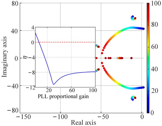
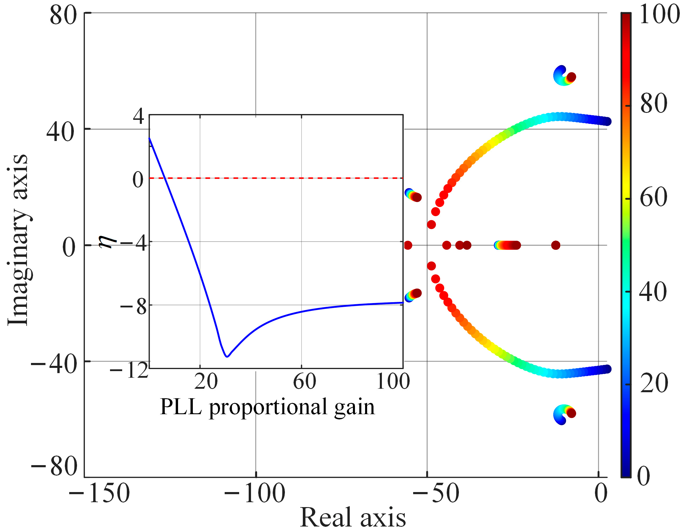
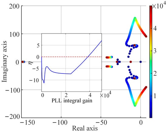
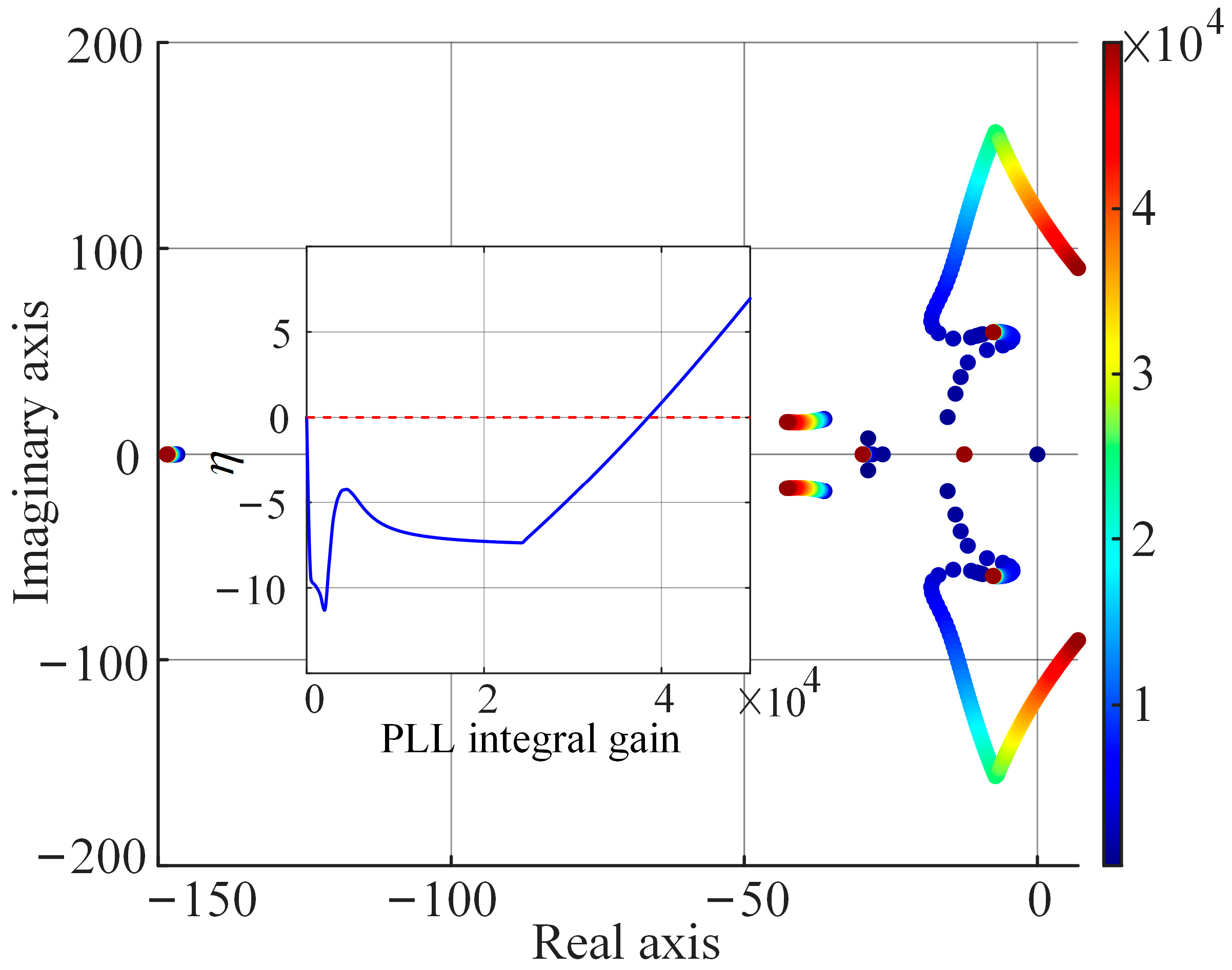
The PLL is a key element affecting synchronization stability in weak grid systems [2,10,11]. At SCR = 2.63, the Floquet characteristic exponent trajectories obtained by separately varying the PLL proportional and integral gains are shown in Figure 6 and Figure 7, respectively. As the proportional gain increases, the critical modes move further into the left half-plane and their damping increases. Variations in the integral gain likewise induce migration of the critical modes; an improper setting may move the corresponding Floquet characteristic exponents into the right half-plane and destabilize the system.

Figure 6. Floquet characteristic exponent trajectories as the PLL proportional gain varies.

Figure 7. Floquet characteristic exponent trajectories as the PLL integral gain varies.

3.2. Impact of Grid Strength on PLL Parameter Stability Region

The preceding subsection separately examines how variations in the PLL proportional and integral gains affect the system’s critical characteristic exponents at a fixed grid strength. In practice, the equivalent grid impedance seen from the PCC varies with network configuration and operating condition. As the grid weakens and its equivalent impedance increases, converter current perturbations produce larger voltage deviations at the PCC. Because the PLL derives its phase information from the positive-sequence PCC voltage, these increased voltage deviations alter the feedback dynamics of the synchronization loop and may shift the critical characteristic exponents. The dependence of the PLL PI parameter stability region on grid strength is therefore evaluated next.

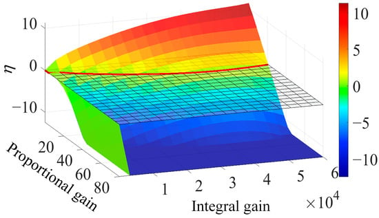
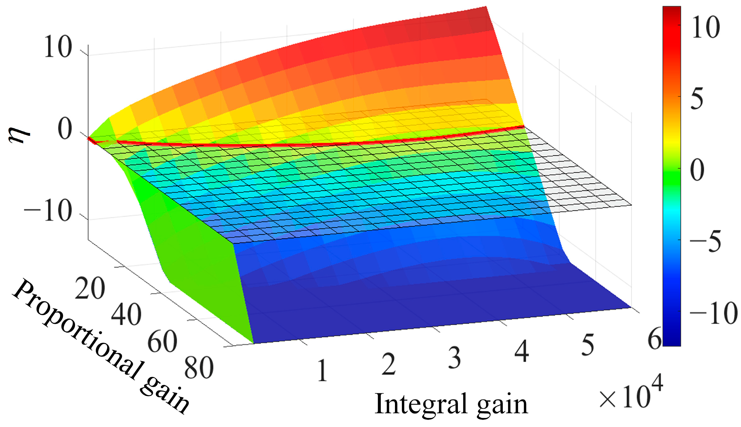
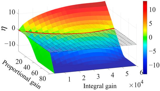
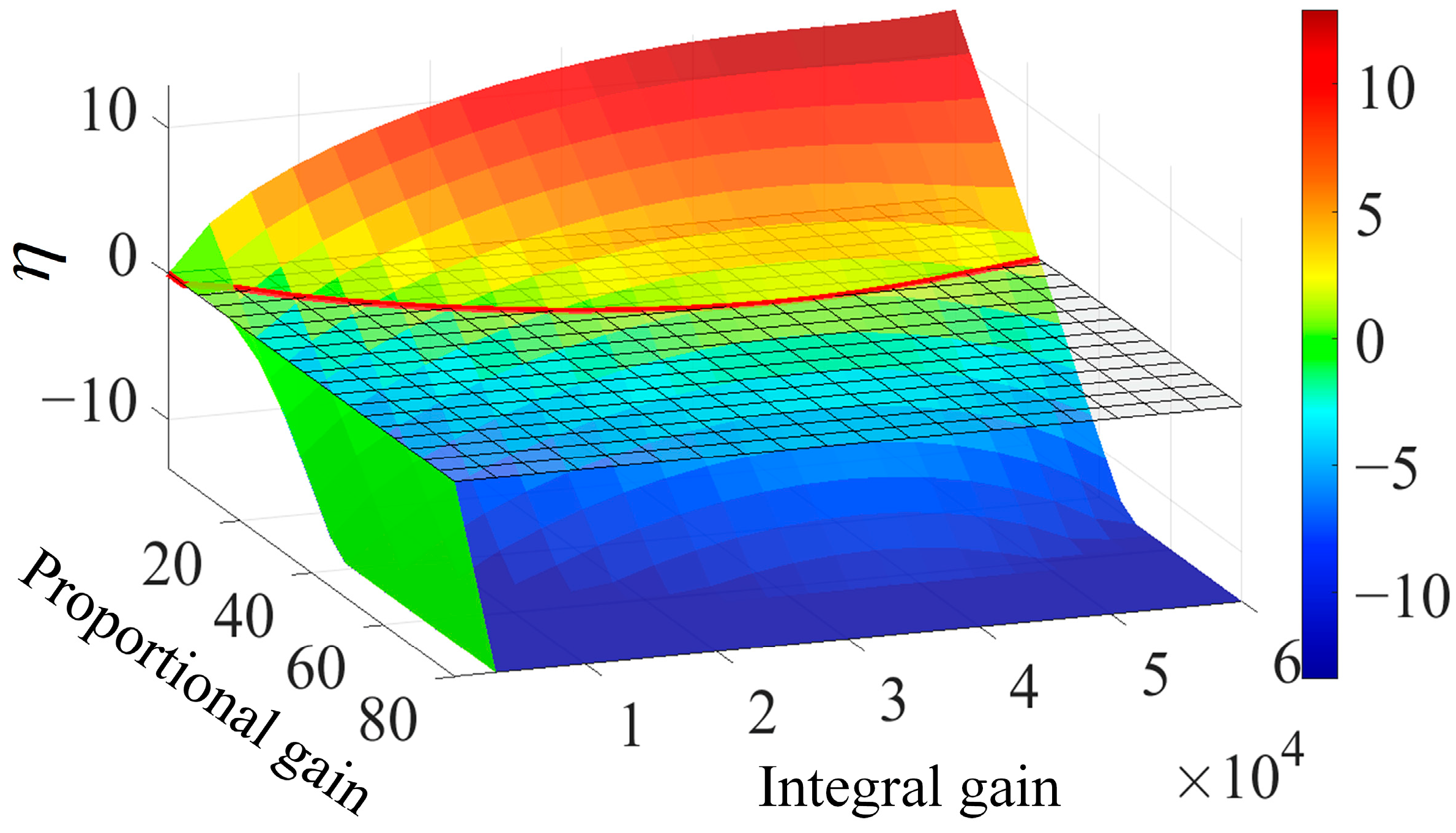
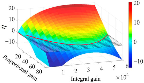
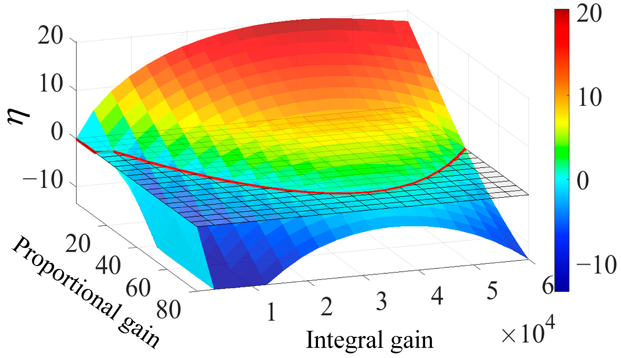
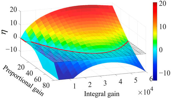
Grid strength is represented by the grid-line inductance L_s. The SCR is calculated using the conventional definition, accounting for both the line and transformer impedances. At L_s = 0.1 p.u., the SCR is approximately 3.57, corresponding to a relatively strong grid; at L_s = 0.2 p.u., the SCR is 2.63, corresponding to a weak grid; at L_s = 0.5 p.u., the SCR is 1.47, which already represents a very weak grid. Accordingly, L_s is increased from 0.2 to 0.5 p.u., with the line resistance adjusted correspondingly and the associated SCR decreasing from 2.63 to 1.47, to examine the PLL parameter stability region under weak to very weak grid conditions. Under each grid condition, k_ppll and k_ipll are swept simultaneously and η is calculated from the complete LTP model. The four three-dimensional stability surfaces corresponding to different grid strengths are shown in Figure 8, Figure 9, Figure 10 and Figure 11 for L_s = 0.2, 0.3, 0.4, and 0.5 p.u., respectively. Parameter combinations satisfying η < 0 form the stable region, while a more negative η indicates a larger distance between the critical exponent and the imaginary axis and hence a greater stability margin.

Figure 8. Stability metric η versus PLL PI parameters for L_s = 0.2 p.u.

Figure 9. Stability metric η versus PLL PI parameters for L_s = 0.3 p.u.

Figure 10. Stability metric η versus PLL PI parameters for L_s = 0.4 p.u.

Figure 11. Stability metric η versus PLL PI parameters for L_s = 0.5 p.u.

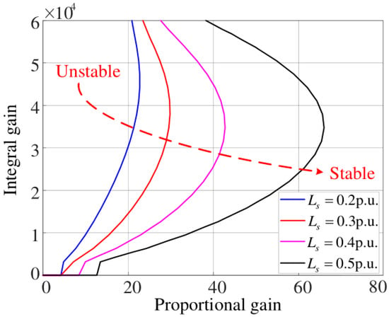
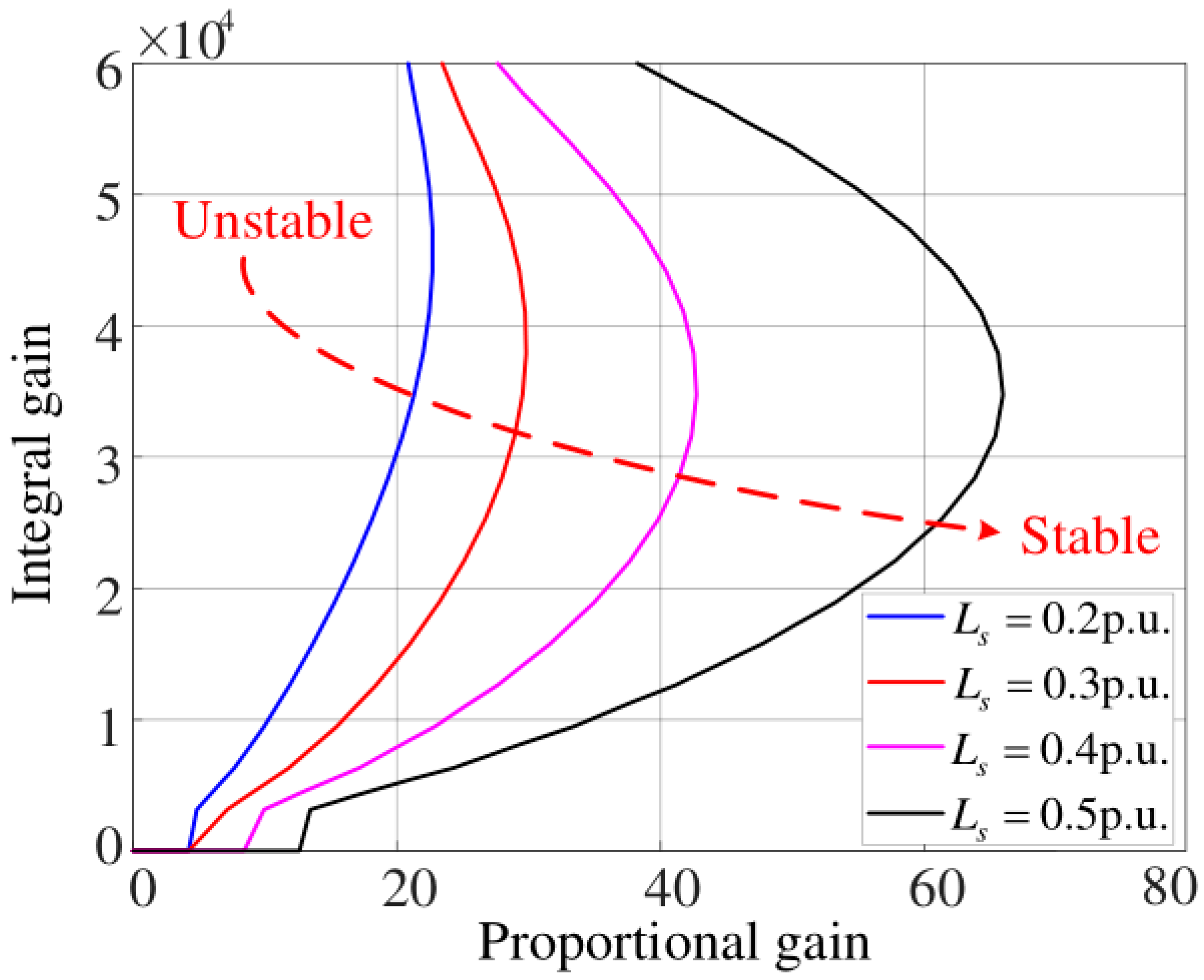
The intersections of the four surfaces with the η = 0 plane are projected onto the PLL PI parameter plane in Figure 12. Each resulting curve corresponds to a specific grid strength and separates the stable and unstable parameter combinations. Within the investigated parameter range, points on the boundary satisfy η = 0, whereas those on the higher-k_ppll side satisfy η < 0 and correspond to asymptotically stable operation. As L_s increases and the SCR decreases, the stability boundary shifts toward higher PLL proportional gains over most of the investigated integral gain range, substantially enlarging the unstable parameter region. Therefore, the PLL gains should be selected according to the minimum anticipated SCR. When the grid strength varies over a specified range, the selected parameter combination should remain within the stability regions corresponding to all anticipated grid conditions, with an appropriate margin from each boundary.

Figure 12. Stability region boundaries of PLL PI parameters under different grid strengths.

4. Virtual Inductance Control Design and Validation

4.1. Identification of the PLL-Dominated Oscillatory Modes

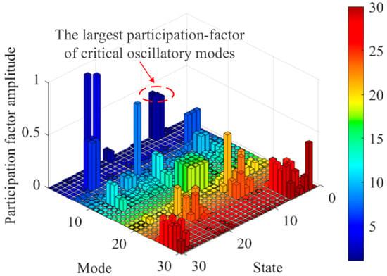
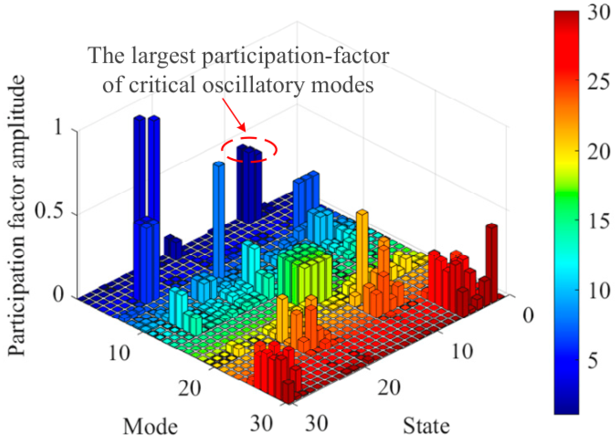
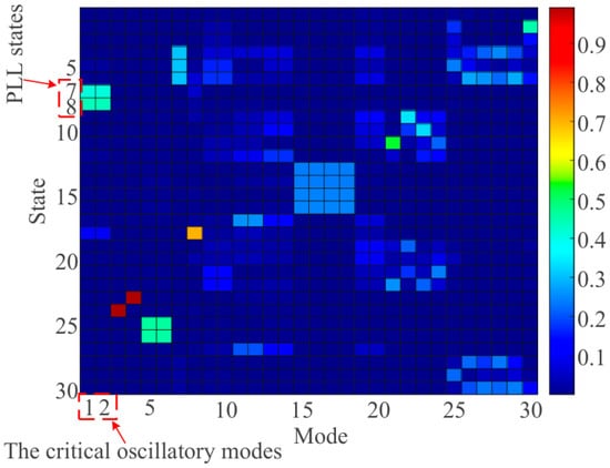
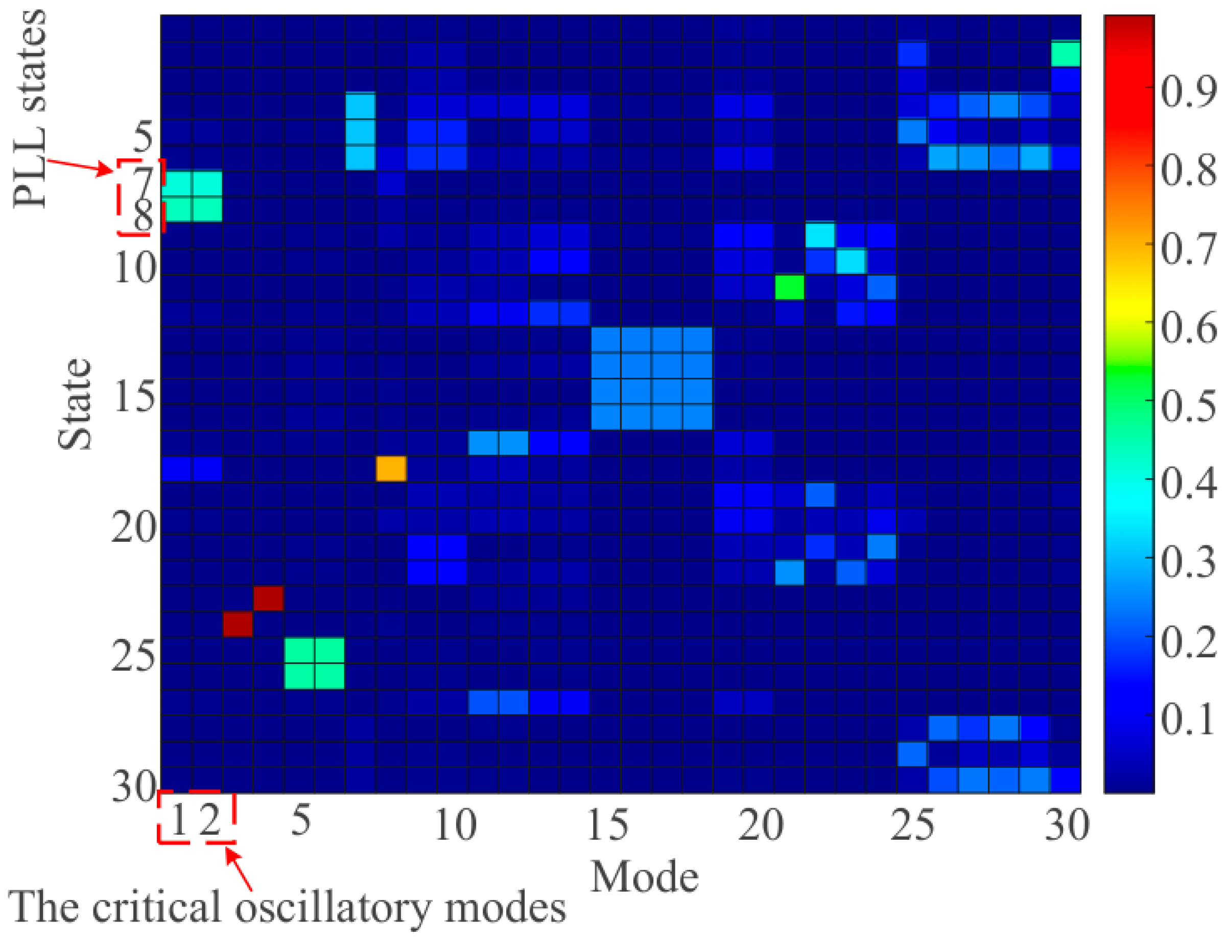
At the weak grid operating point with SCR = 1.47, the participation factors are evaluated to determine the states most strongly associated with the critical oscillatory mode. For the k-th Floquet mode and the i-th state, the participation factor is defined as

p_ik = r_ikl_ki,

(22)

where r_ik and l_ki denote the i-th entries of the right and left eigenvectors associated with mode k, respectively. The magnitudes of the complete participation factor matrix are presented as a three-dimensional distribution in Figure 13 and as a heat map in Figure 14.

Figure 13. Participation factor magnitudes at SCR = 1.47: three-dimensional distribution.

Figure 14. Participation factor magnitudes at SCR = 1.47: heat map.

Specifically, state 7 corresponds to the integrator output of the PLL PI controller, whereas state 8 corresponds to the output of the second PLL integrator and represents the PLL angle state. For the critical conjugate oscillatory modes (modes 1 and 2), the participation factor magnitudes associated with states 7 and 8 are approximately 0.3995 and 0.4330, respectively. For the critical oscillatory modes, the largest participation factor magnitudes are associated with the PLL states, indicating that the modes are dominated by PLL dynamics. This finding provides the basis for modifying the PLL synchronization voltage path to introduce additional damping.

4.2. Virtual PCC Equivalent Circuit and Control Principle

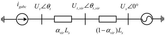
Weak grid operation strengthens the interaction between the converter control system and the physical grid impedance. Several approaches are available to enhance weak grid stability, including virtual inductance control and adaptive gain scheduling. In this study, virtual inductance control is selected to construct a virtual PCC voltage for PLL synchronization. This choice is motivated by the PLL-dominated oscillatory mode identified in Section 4.1. By modifying the PLL synchronization voltage path, this method improves the damping of the identified mode while retaining the existing PLL gains and the original voltage and current control structures. The corresponding equivalent circuit is shown in Figure 15.

Figure 15. The equivalent circuit of the grid-connected PV system using a virtual PCC voltage.

In Figure 15, the measured PCC voltage U_t ∠ θ_t and the virtual voltage U_t,vir ∠ θ_t,vir define an equivalent division of the physical grid inductance L_s into α_virL_s and (1 − α_vir)L_s. This representation does not introduce a physical inductor; instead, it represents an equivalent shift of the PLL synchronization point produced by modifying the measured voltage [10]. The positive-sequence q-axis voltage supplied to the PLL is given by

u_tq+,vir = u_tq+ − ω_pllα_virL_si_gd+,0 ≤ α_vir ≤ 1,

(23)

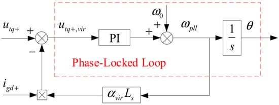
where u_tq+ is the positive-sequence q-axis PCC voltage, i_gd+ is the positive-sequence d-axis component of the converter output current, ω_pll = ω₀ + ω_s is the angular frequency estimated by the PLL, and α_vir is the dimensionless virtual inductance coefficient, with 0 ≤ α_vir ≤ 1. With i_g defined as positive from the converter toward the grid, the current-dependent voltage term in (23) is subtracted from u_tq+. When α_vir = 0, the virtual PCC voltage equals the measured PCC voltage, and the virtual inductance control path is inactive. As α_vir increases, the magnitude of this compensation term grows, reducing the positive-sequence q-axis component of the virtual PCC voltage. Its effect on the damping of the PLL-dominated mode is evaluated in Section 4.3. In the present study, Equation (23) is evaluated under ideal measurement conditions, with sensor noise and delays in the measurement and compensation paths neglected. The effects of these nonidealities on the proposed control are not evaluated, which constitutes a limitation of the present study. The corresponding implications and future research directions are discussed in Section 6.

Figure 16 shows the implementation of the virtual inductance control. Because the added control path acts only on the virtual voltage used for PLL synchronization, the original DVC, TVC, and ACC structures remain unchanged.

Figure 16. Block diagram of virtual inductance control.

4.3. Control Coefficient Selection and Damping Validation

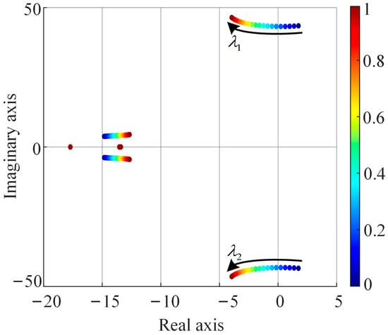
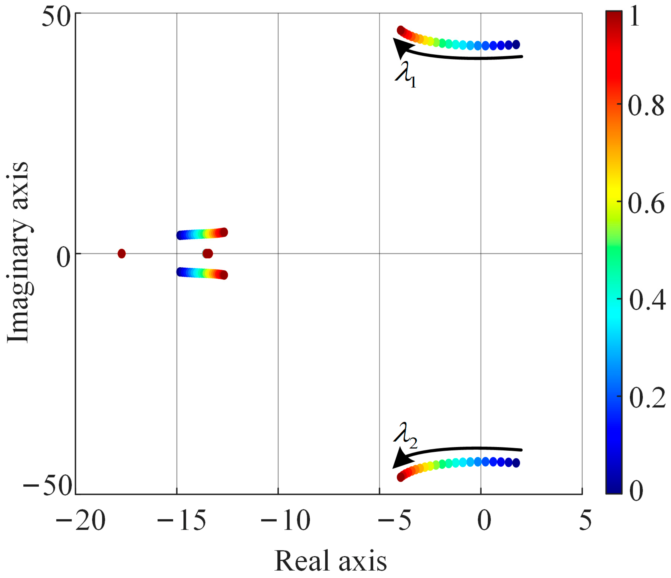
To test the damping mechanism, k_ppll is set to five so that the system is unstable, and α_vir is swept from zero toward unity. As shown in Figure 17, increasing α_vir moves the PLL-associated characteristic exponent pair monotonically toward the left half-plane. The pair crosses the imaginary axis at α_vir ≈ 0.25, indicating recovery of small-signal stability. Although several noncritical modes move slightly rightward, their real parts remain negative throughout the investigated interval and do not determine the stability boundary. Thus, under the investigated operating condition, the stable interval extends from just above α_vir ≈ 0.25 to α_vir = 1. Within the identified stable interval, α_vir = 0.4 is selected as a representative value for subsequent analysis of virtual inductance control and validation of its effectiveness. In this setting, all characteristic exponents have real parts below −1 s⁻¹, indicating a finite small-signal stability margin.

Figure 17. Floquet characteristic exponent trajectories as virtual inductance coefficient α_vir varies.

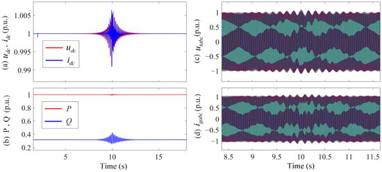
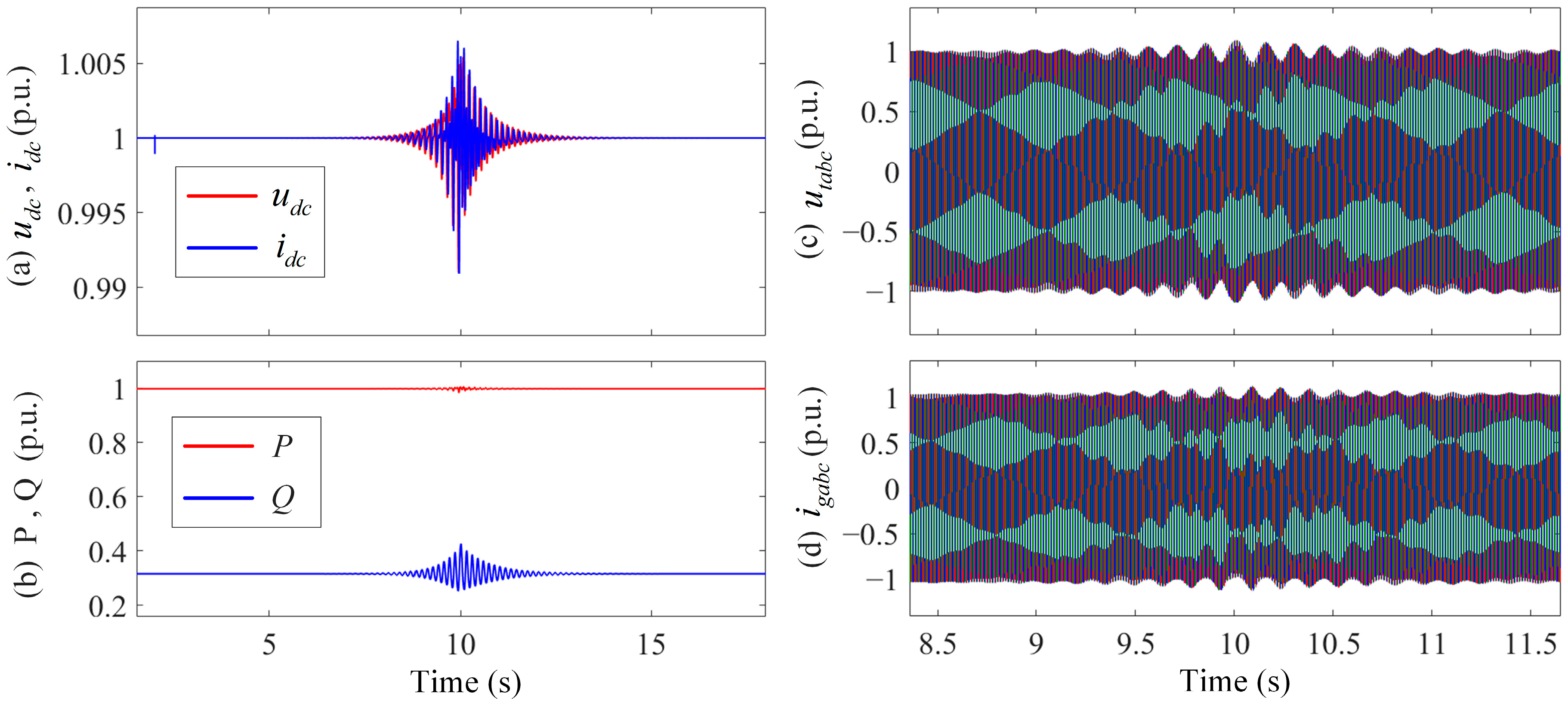
The damping effect of the proposed control is verified with a nonlinear EMT model. At t = 2 s, the PLL proportional gain is changed from a stable operating value to 5, causing instability; the virtual inductance control is activated at t = 10 s. Figure 18 presents the DC-link voltage u_dc, DC-link current i_dc, active power P, reactive power Q, three-phase PCC voltage u_tabc, and three-phase converter current i_gabc. Before activation, the oscillation amplitudes of the DC- and AC-side electrical quantities increase continuously. After the control is activated, all oscillation amplitudes decay and the system returns to its periodic steady state. The nonlinear time-domain response confirms the effectiveness of the proposed virtual inductance control strategy in suppressing PLL-dominated oscillations.

Figure 18. System time-domain responses before and after activation of virtual inductance control during oscillatory instability. (a) The DC-link voltage u_dc and current i_dc. (b) The active power P and reactive power Q. (c) The three-phase PCC voltage u_tabc. (d) The three-phase converter current i_gabc.

4.4. Expansion of the PLL Parameter Stability Region

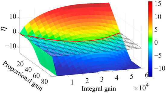
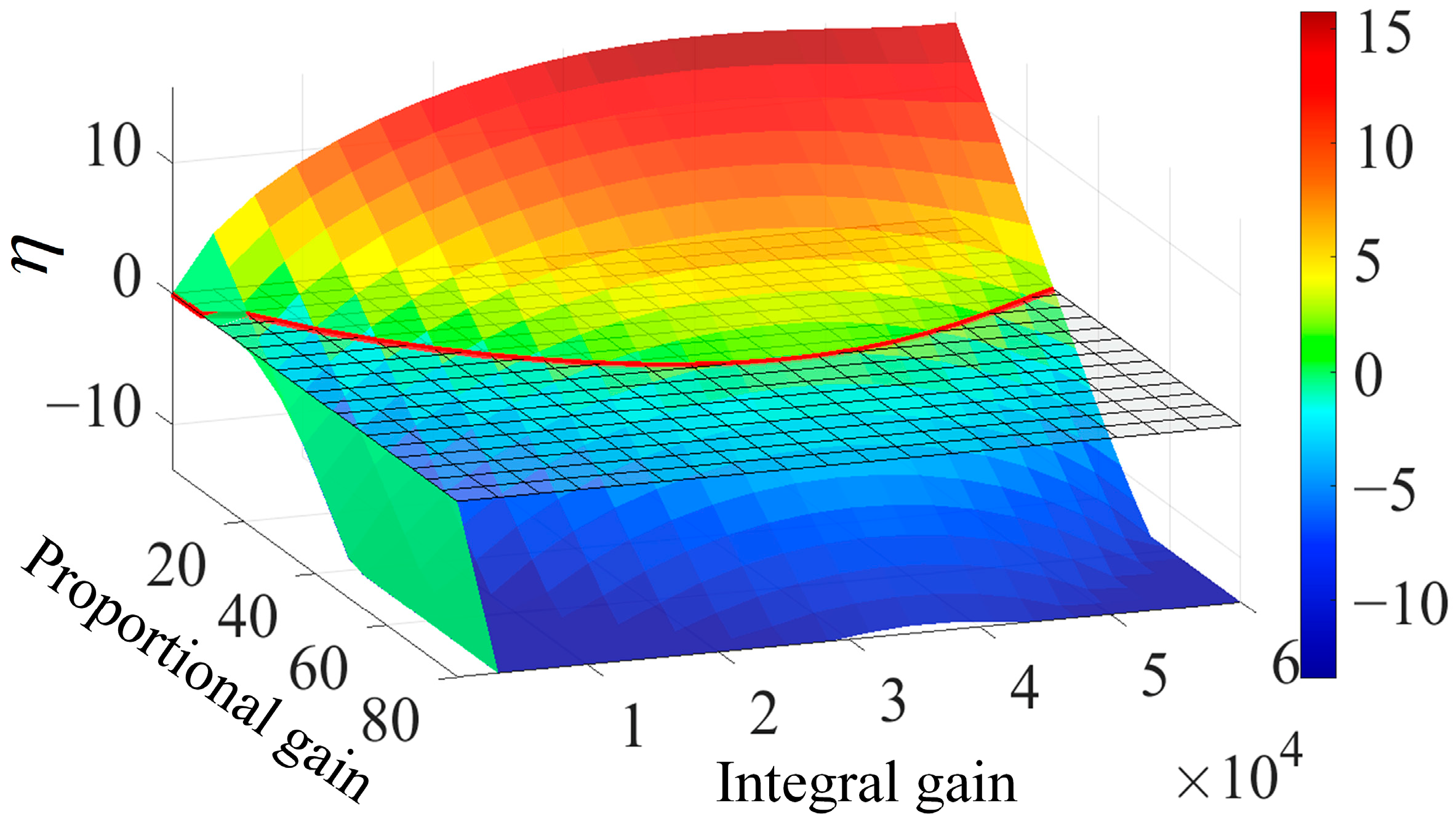
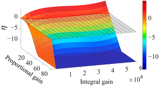
The preceding tests demonstrate damping in one deliberately unstable PLL setting. To assess the PLL parameter stability region over a wider range of gain combinations, k_ppll and k_ipll are swept simultaneously under the same weak grid condition. For the cases without virtual inductance control and with virtual inductance control (α_vir = 0.4), the stability metric η is recalculated for every parameter pair. The two cases are presented separately in Figure 19 and Figure 20.

Figure 19. Stability metric η versus PLL PI parameters without virtual inductance control.

Figure 20. Stability metric η versus PLL PI parameters with virtual inductance control (α_vir = 0.4).

Without virtual inductance control, Figure 19 contains a broad positive-η region and the admissible PLL gains are strongly constrained. With α_vir = 0.4, the negative-η basin in Figure 20 extends over a substantially larger portion of the gain plane. This comparison shows that the control does more than stabilize the single k_ppll = 5 test case: it enlarges the set of PLL proportional and integral gain combinations that yield stable operation under the investigated grid condition.

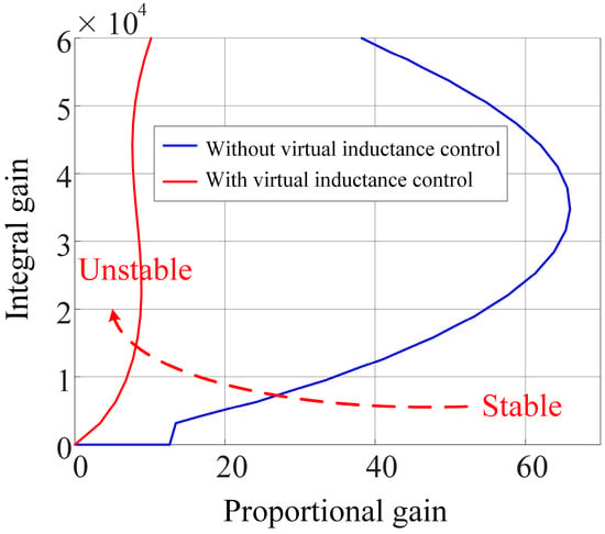
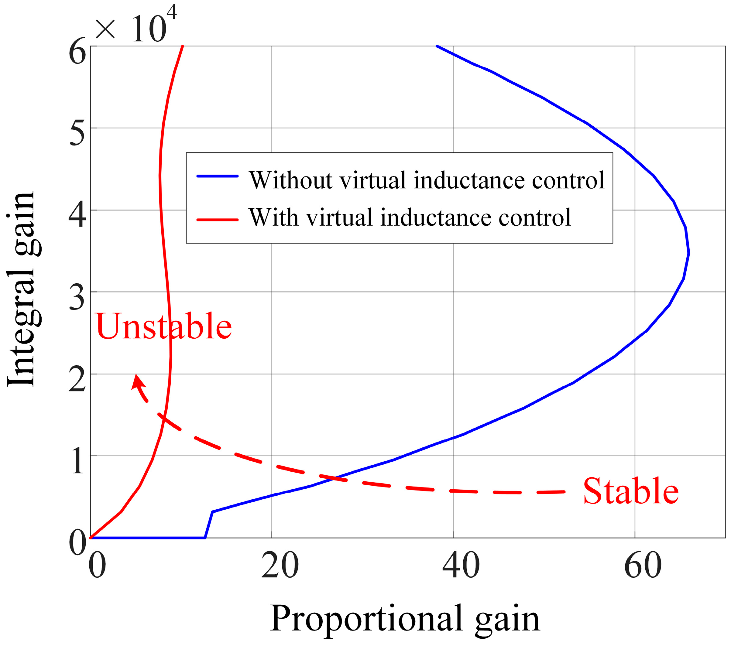
For a direct comparison, the η = 0 intersections of the two surfaces are projected onto the PLL gain plane in Figure 21. The two curves represent the boundaries between stable and unstable parameter combinations before and after activation of virtual inductance control.

Figure 21. Stability region boundaries of PLL PI parameters with and without virtual inductance control.

As Figure 21 shows, activating the virtual inductance control moves the boundary toward lower gains and markedly reduces the unstable portion of the parameter plane. The set of stable PLL gain combinations therefore expands within the investigated parameter range. This enlargement provides greater flexibility in selecting PLL gains under the studied weak grid condition.

5. Results

The numerical results corresponding to the three contributions stated in Section 1 are presented below.

(1)

Quantitative validation of the LTP small-signal model

Figure 3, Figure 4 and Figure 5 compare the time-domain responses of the LTP and nonlinear EMT models under a DC-link voltage reference perturbation of +0.02 p.u., a grid frequency perturbation of +0.1 Hz, and a balanced three-phase voltage sag of 0.01 p.u., respectively. Each disturbance is applied at 2 s and removed at 2.1 s. The validation is conducted at L_s = 0.2 p.u. and SCR = 2.63, with PLL proportional and integral gains of 50 and 2000, respectively. The two models show close agreement during both the application and removal of the disturbances.

The quantitative error metrics evaluated over 2–2.8 s are reported in Table A2 of Appendix A. For the DC-link voltage reference perturbation, the RMSE and MaxAbsError of u_dc are 8.61 × 10⁻⁵ p.u. and 3.19 × 10⁻⁴ p.u., respectively. For the grid frequency perturbation, the corresponding errors of the PLL frequency f are 3.39 × 10⁻⁵ Hz and 1.15 × 10⁻⁴ Hz. For the voltage sag, the corresponding errors of the phase-A PCC voltage u_ta are 2.11 × 10⁻⁵ p.u. and 1.23 × 10⁻⁴ p.u. Overall, the RMSE and MaxAbsError values in Table A2 are small for all observed quantities under the three disturbance scenarios. These results quantitatively validate the accuracy of the developed LTP model in representing the DC-side, PLL, and AC-side dynamic responses under the investigated disturbances.

(2)

Stability analysis of PLL parameters and grid strength, and identification of the critical oscillatory modes

At SCR = 2.63, the characteristic exponent trajectories in Figure 6 and Figure 7 show how variations in the PLL proportional and integral gains affect the critical modes. Within the investigated parameter range, increasing the proportional gain moves the critical modes further into the left half-plane and increases their damping. Changing the integral gain likewise induces migration of the critical modes, while an improper integral gain setting may move the critical characteristic exponents into the right half-plane.

The grid strength analysis considers four conditions with L_s = 0.2, 0.3, 0.4, and 0.5 p.u., with the SCR decreasing from 2.63 to 1.47. Figure 8, Figure 9, Figure 10, Figure 11 and Figure 12 show that, as the grid weakens, the stability boundary shifts toward higher PLL proportional gains over most of the investigated integral gain range, reducing the stable parameter region.

Under the very weak grid condition with SCR = 1.47, the participation factor results in Figure 13 and Figure 14 identify states 7 and 8 as the dominant contributors to the critical conjugate oscillatory modes (modes 1 and 2). Their participation factor magnitudes are approximately 0.3995 and 0.4330, respectively. These magnitudes are substantially higher than those of the other states for the same critical oscillatory mode pair. The two states correspond to the PLL PI integrator output and PLL angle state, respectively, establishing a quantitative association between the critical oscillatory modes and the internal PLL dynamics.

(3)

Oscillation suppression and stability region expansion using virtual inductance control

The PLL proportional gain is set to 5 under the investigated very weak grid condition. Figure 17 shows that increasing α_vir moves the PLL-associated characteristic exponent pair toward the left half-plane. The pair crosses the imaginary axis at approximately α_vir = 0.25, and small-signal stability is maintained for control coefficient values from just above this boundary to α_vir = 1. At the representative setting α_vir = 0.4, all characteristic exponents have real parts below −1 s⁻¹, indicating a positive stability margin.

The nonlinear EMT responses in Figure 18 provide further validation of the control effectiveness. Changing the PLL proportional gain to 5 at 2 s produces oscillations with continuously increasing amplitudes. After virtual inductance control is activated at 10 s, the oscillation amplitudes decay and the system returns to its periodic steady state. Furthermore, Figure 19, Figure 20 and Figure 21 show that, with α_vir = 0.4, the stability boundary shifts toward lower gains and the PLL PI parameter stability region expands. These results demonstrate that virtual inductance control both suppresses the identified PLL-dominated oscillations and enlarges the set of PLL gain combinations that yield stable operation under the investigated grid condition.

6. Discussion

The close agreement between the LTP model developed in this study and the nonlinear EMT model supports Floquet-based stability analysis using the developed model under the investigated operating conditions. The parameter sweep results show that variations in the PLL proportional and integral gains produce different migration patterns of the critical characteristic exponents. As the grid weakens, the stability boundary shifts toward higher proportional gains over most of the investigated integral gain range, reducing the stable parameter region. This finding is consistent with previous research on the influence of grid conditions on the small-signal stability boundaries of grid-following converters [13]. It also indicates that PLL parameters selected under stronger grid conditions may become unsuitable as the SCR decreases.

The participation factor results identify the PLL states as the dominant contributors to the critical oscillatory modes. The importance of internal PLL dynamics is consistent with previous findings on modal resonance between the PLL and DC-link voltage control under weak grid conditions [6]. Accordingly, virtual inductance control is adopted on the basis of the identified PLL-dominated modes to modify the voltage used for PLL synchronization through a current-dependent compensation term. The observed oscillation decay and expansion of the stable parameter region indicate that this voltage modification improves the damping of the PLL-dominated modes while retaining the original voltage and current control structures.

Several limitations should be considered when interpreting these findings. First, the PV array is represented by an ideal controlled current source, and MPPT dynamics are not explicitly modeled. This approximation follows a qualitative multi-time-scale modeling rationale under constant irradiance and temperature [25]. However, the assumed time-scale separation has not been quantitatively verified using a full model incorporating PV array characteristics and MPPT control. Research under rapidly varying irradiance indicates that MPPT dynamics may affect DC-link voltage regulation and transient response [24]. Future studies should therefore incorporate the PV array current–voltage characteristics and explicit MPPT dynamics to assess their coupling with the DC-link voltage controller and PLL.

Second, virtual inductance control is evaluated under ideal measurement conditions, with sensor noise and delays in the measurement and compensation paths neglected. Noise in the measured voltage and current signals may propagate into the virtual PCC voltage and affect PLL synchronization, while delays may introduce phase lag and alter the damping provided by the compensation. Consequently, the present results establish control effectiveness under the adopted ideal conditions, while robustness to these implementation effects remains to be assessed. Future work should incorporate measurement noise and implementation delays into the analysis, evaluate their influence on modal damping and stability boundaries, and investigate appropriate filtering and delay compensation strategies.

Third, the analyses of control effectiveness and the control coefficient are based on the selected system and operating conditions, and the applicability of the findings to broader scenarios requires further evaluation. Related research has examined transient stability between grid-following doubly fed induction generator wind turbines and grid-forming converters on the electromechanical time scale [26], illustrating the broader range of system configurations considered in converter-related stability studies. Future studies should extend the present analysis to a broader range of operating scenarios. The stable range of the virtual inductance coefficient identified in this study is specific to the investigated operating point, and α_vir = 0.4 is a representative selection rather than a universally optimal value. Further research should assess how the control coefficient affects modal damping and stability margins as grid conditions and controller parameters vary, providing a basis for coefficient selection under different operating conditions.

Finally, the relative performance of virtual inductance control against other weak grid stabilization methods has not been quantitatively assessed in this study. A comprehensive comparison of different weak grid stabilization methods is therefore an important direction for future research.

7. Conclusions

The main conclusions of this study are summarized as follows:

(1)

An LTP small-signal model incorporating SOGI-based positive-/negative-sequence separation and negative-sequence current control was developed. Its accuracy was validated against a nonlinear EMT model under three disturbance conditions.

(2)

Floquet characteristic exponent analysis reveals different critical-mode migration patterns as the PLL proportional and integral gains vary. As the SCR decreases, the stable region in the PLL PI parameter plane contracts.

(3)

Participation factor analysis identifies the critical oscillatory modes as PLL dominates. Under the investigated operating conditions, virtual inductance control suppresses PLL-dominated oscillations and enlarges the PLL PI parameter stability region.

References

- Jia, Q.; Yan, G.; Cai, Y.; Li, Y.; Zhang, J. Small-signal stability analysis of photovoltaic generation connected to weak AC grid. J. Mod. Power Syst. Clean Energy 2019, 7, 254–267. [Google Scholar] [CrossRef] [Scilit]
- Huang, Y.; Yuan, X.; Hu, J.; Zhou, P. Modeling of VSC connected to weak grid for stability analysis of DC-link voltage control. IEEE J. Emerg. Sel. Top. Power Electron. 2015, 3, 1193–1204. [Google Scholar] [CrossRef] [Scilit]
- Wang, X.; Blaabjerg, F. Harmonic stability in power electronic-based power systems: Concept, modeling, and analysis. IEEE Trans. Smart Grid 2019, 10, 2858–2870. [Google Scholar] [CrossRef] [Scilit]
- Zhu, L.; Liu, Y.; Wang, P.; Chen, J.; Jia, Q.; Jia, G. Synchronous stability analysis and enhancement method for grid connected inverters in weak grids. Sci. Rep. 2026, 16, 26385. [Google Scholar] [CrossRef] [Scilit] [PubMed]
- Nguyen, T.B.; Arkhincheev, V. Optimal placement of solar photovoltaic systems and electric vehicle charge stations in distribution power grids, considering the constraints of areas and locations. J. Adv. Eng. Comput. 2026, 10, 217–232. [Google Scholar] [CrossRef] [Scilit]
- Wang, D.; Liang, L.; Shi, L.; Hu, J.; Hou, Y. Analysis of modal resonance between PLL and DC-link voltage control in weak-grid tied VSCs. IEEE Trans. Power Syst. 2019, 34, 1127–1138. [Google Scholar] [CrossRef] [Scilit]
- Liao, Y.; Wang, X. Small-signal modeling of AC power electronic systems: Critical review and unified modeling. IEEE Open J. Power Electron. 2021, 2, 424–439. [Google Scholar] [CrossRef] [Scilit]
- Liao, Y.; Wang, X.; Yue, X.; Harnefors, L. Complex-valued multifrequency admittance model of three-phase VSCs in unbalanced grids. IEEE J. Emerg. Sel. Top. Power Electron. 2020, 8, 1934–1946. [Google Scholar] [CrossRef] [Scilit]
- Rygg, A.; Molinas, M.; Zhang, C.; Cai, X. A modified sequence-domain impedance definition and its equivalence to the dq-domain impedance definition for the stability analysis of AC power electronic systems. IEEE J. Emerg. Sel. Top. Power Electron. 2016, 4, 1383–1396. [Google Scholar] [CrossRef] [Scilit]
- Suul, J.A.; D’Arco, S.; Rodríguez, P.; Molinas, M. Impedance-compensated grid synchronisation for extending the stability range of weak grids with voltage source converters. IET Gener. Transm. Distrib. 2016, 10, 1315–1326. [Google Scholar] [CrossRef] [Scilit]
- Golestan, S.; Guerrero, J.M.; Vasquez, J.C. Three-phase PLLs: A review of recent advances. IEEE Trans. Power Electron. 2017, 32, 1894–1907. [Google Scholar] [CrossRef] [Scilit]
- Wu, H.; Wang, X.; Wang, K.; Li, G.; Zhang, B.; Lu, Y. Passivity-based harmonic stability analysis of voltage source converters considering the impact of sequence decomposition algorithms. In Proceedings of the 2020 IEEE 9th International Power Electronics and Motion Control Conference (IPEMC2020-ECCE Asia), Nanjing, China, 29 November–2 December 2020; IEEE: Piscataway, NJ, USA, 2020; pp. 1930–1934. [Google Scholar] [CrossRef] [Scilit]
- Liu, G.; Starke, M. A state-space model for stability boundary analysis of grid-following voltage source converters considering grid conditions. Energies 2026, 19, 1521. [Google Scholar] [CrossRef] [Scilit]
- Daryabak, M.; Filizadeh, S.; Jatskevich, J.; Davoudi, A.; Saeedifard, M.; Sood, V.K.; Martinez, J.A.; Aliprantis, D.; Cano, J.; Mehrizi-Sani, A. Modeling of LCC-HVDC systems using dynamic phasors. IEEE Trans. Power Deliv. 2014, 29, 1989–1998. [Google Scholar] [CrossRef] [Scilit]
- Sakinci, O.C.; Beerten, J. Generalized dynamic phasor modeling of the MMC for small-signal stability analysis. IEEE Trans. Power Deliv. 2019, 34, 991–1000. [Google Scholar] [CrossRef] [Scilit]
- Kwon, J.B.; Wang, X.; Blaabjerg, F.; Bak, C.L.; Sularea, V.-S.; Busca, C. Harmonic interaction analysis in a grid-connected converter using harmonic state-space (HSS) modeling. IEEE Trans. Power Electron. 2017, 32, 6823–6835. [Google Scholar] [CrossRef] [Scilit]
- Zhu, J.; Guo, Z.; Hu, J.; Ma, S.; Guo, J. Truncation number selection of harmonic state-space model based on the Floquet characteristic exponent. IEEE Trans. Ind. Electron. 2023, 70, 3222–3228. [Google Scholar] [CrossRef] [Scilit]
- Salis, V.; Costabeber, A.; Cox, S.M.; Zanchetta, P. Stability assessment of power-converter-based AC systems by LTP theory: Eigenvalue analysis and harmonic impedance estimation. IEEE J. Emerg. Sel. Top. Power Electron. 2017, 5, 1513–1525. [Google Scholar] [CrossRef] [Scilit]
- Yang, H.; Just, H.; Eggers, M.; Dieckerhoff, S. Linear time-periodic theory-based modeling and stability analysis of voltage-source converters. IEEE J. Emerg. Sel. Top. Power Electron. 2021, 9, 3517–3529. [Google Scholar] [CrossRef] [Scilit]
- Li, H.; Liu, C.; Jiang, X.; Zeng, Y.; Guo, Z.; Zheng, T.Q. A time-domain stability analysis method for grid-connected inverter with PR control based on Floquet theory. IEEE Trans. Ind. Electron. 2021, 68, 11125–11134. [Google Scholar] [CrossRef] [Scilit]
- Montagnier, P.; Spiteri, R.J.; Angeles, J. The control of linear time-periodic systems using Floquet–Lyapunov theory. Int. J. Control 2004, 77, 472–490. [Google Scholar] [CrossRef] [Scilit]
- Hu, J.; Guo, Z.; Zhu, J.; Kurths, J.; Hou, Y.; Du, B.; Wu, Z.; Zhao, G.; Liu, Y.; Xin, K.; et al. Electromagnetic dynamic stability analysis of power electronics-dominated systems using eigenstructure-preserved LTP theory. Nat. Commun. 2025, 16, 6852. [Google Scholar] [CrossRef] [Scilit] [PubMed]
- Guo, Z.; Zhu, J.; Hu, J.; Zhao, G.; Wu, Z.; Du, B.; Guo, J. HSS eigenvalue sensitivity for small-signal stability analysis of nonlinear time-periodic system. IEEE Trans. Power Electron. 2025, 40, 4762–4766. [Google Scholar] [CrossRef] [Scilit]
- Big-Alabo, A. Analyses of deep reinforcement learning and conventional MPPT control under fast-changing irradiance. J. Adv. Eng. Comput. 2026, 10, 13–35. [Google Scholar] [CrossRef] [Scilit]
- Yuan, X.; Hu, J.; Cheng, S. Multi-time scale dynamics in power electronics-dominated power systems. Front. Mech. Eng. 2017, 12, 303–311. [Google Scholar] [CrossRef] [Scilit]
- Tang, W.; Zheng, W.; Zhou, B.; Yang, Z.; Zhang, Y. Transient stability analysis between grid-following DFIG-WT and grid-forming converter in electromechanical timescale. IEEE Trans. Energy Convers. 2025, 40, 2485–2495. [Google Scholar] [CrossRef] [Scilit]
Disclaimer/Publisher’s Note: The statements, opinions and data contained in all publications are solely those of the individual author(s) and contributor(s) and not of MDPI and/or the editor(s). MDPI and/or the editor(s) disclaim responsibility for any injury to people or property resulting from any ideas, methods, instructions or products referred to in the content. |
© 2026 by the authors. Licensee MDPI, Basel, Switzerland. This article is an open access article distributed under the terms and conditions of the Creative Commons Attribution (CC BY) license.