Operational Factors Associated with Saline Activated Sludge Performance: Insights from Explainable Machine Learning

Abstract

Numerous studies have explored how environmental and process parameters shape microbial community composition in activated sludge. However, a critical gap remains in identifying which operational and environmental conditions are most strongly associated with microbiome characteristics linked to wastewater treatment performance, particularly under real-world operational conditions where multiple variables exert simultaneous and interacting influences. In this study, we leverage high-throughput metatranscriptomic data combined with machine learning–based feature selection to identify the most informative measured process and environmental parameters associated with activated sludge microbiome structure of highest removal performance. Unlike traditional approaches that rely on controlled laboratory experiments with replicated conditions, our method enables the analysis of complex, full-scale systems without the need for extensive experimental replication, thereby capturing the intrinsic variability of real-world wastewater treatment processes. Using data from a saline wastewater treatment plant which was previously shown to benefit from microbial communities with high functional gene diversity and evenness, we evaluated the relative importance of measured operational variables. Recursive feature elimination, using a Random Forest model with repeated 10-fold cross-validation, identified blower operational load, mixed liquor suspended solids, and temperature as the most informative predictors of functional gene diversity among the operational and environmental variables evaluated.

1. Introduction

The activated sludge microbiome is integral to the functionality of wastewater treatment plants (WWTPs), serving as a dynamic microbial community responsible for organic matter degradation, nutrient removal, and pollutant degradation [1]. However, the operational efficiency of this microbiome is heavily influenced by environmental and process parameters such as temperature, pH, oxygen concentration, and hydraulic retention time [2]. Understanding how these operational and environmental factors relate to microbial community structure and function is critical for optimizing wastewater treatment processes and addressing global water management challenges [3]. Additionally, insights derived from studying these relationships can have broad applications in fields such as bioremediation, agricultural microbiome management, and industrial biotechnology, thereby yielding significant environmental and economic benefits [4,5].

Activated sludge is a well-established biological secondary-treatment process in which wastewater is brought into contact with a concentrated microbial biomass under controlled aeration and mixing. Microorganisms convert biodegradable organic matter and nutrients, after which the biomass is separated from treated water by sedimentation; a fraction of the settled sludge is returned to maintain the active microbial population, while excess sludge is removed [1]. At full scale, treatment performance therefore emerges from the combined effects of influent characteristics, organic and nutrient loading, aeration and dissolved-oxygen conditions, biomass concentration, sludge retention, hydraulic conditions, temperature, and other operating variables. These variables can change simultaneously during routine plant operation, making the biological state of a full-scale activated sludge system considerably more heterogeneous than conditions typically imposed in controlled laboratory experiments [1].

Scientific studies have examined the effects of individual operational and environmental parameters on activated sludge using a range of controlled experimental systems. Prawira Negara et al. [6] investigated glycerol loading in laboratory-scale reactors designed to mimic an industrial saline wastewater treatment plant, assessing COD and nitrogen removal together with changes in microbial community composition. Meynet et al. [7] evaluated long-term temperature shifts (4–40 °C) in sequencing batch reactors, focusing on activated sludge microbial dynamics and micropollutant biotransformation. Aimale-Troy et al. [8] studied dissolved oxygen concentrations of 1–8 mg L⁻¹ in a laboratory-scale sequencing batch reactor supplied with synthetic wastewater, evaluating bacterial community structure, oxygen uptake rate, and COD removal. Similarly, Jin et al. [9] investigated dissolved oxygen effects in integrated fixed-film activated sludge sequencing batch reactors, focusing on simultaneous nitrification–denitrification performance and associated microbial pathways. Collectively, these studies demonstrate the value of controlled reactor and batch systems for resolving the effects of specific variables; however, they generally manipulate one or a limited number of factors at a time. In contrast, full-scale WWTPs operate under simultaneous variation in influent composition, loading, aeration, temperature, biomass concentration, and other process conditions, making it important to determine the relative predictive importance of these variables under real operational conditions. Although the individual effects of operational parameters such as temperature, aeration, organic loading, and biomass concentration are well established, their relative importance under full-scale operating conditions is less clearly resolved. Consequently, an important unresolved question is not simply whether individual parameters affect activated sludge, but which measured variables have the greatest relative predictive importance under real operational conditions. This distinction is important because variables known individually to affect activated sludge do not necessarily have equal predictive importance when they fluctuate concurrently in an industrial treatment system.

Recent advancements in molecular technologies, including high-throughput sequencing and meta’omics, have revolutionized the field by enabling detailed profiling of microbial communities at the species and genus levels [10,11,12]. These techniques enable investigation of how environmental and process parameters are associated with microbial community composition and functional potential [13,14,15,16]. For example, studies have shown that shifts in temperature and dissolved oxygen concentrations can alter the abundance of microbial groups involved in nitrogen and carbon cycling, subsequently influencing microbiome dynamics and treatment efficiency [17,18,19]. In addition, advanced machine learning techniques were employed to elucidate the collective effects of environmental variables on activated sludge microbial communities at a global scale according to the similarity of microbial community structure [20]. Recent full-scale studies have likewise demonstrated that operational factors are associated with variation in activated-sludge community composition [21]. However, identifying whether a parameter affects microbial communities is conceptually different from determining its relative predictive importance when multiple operational and environmental variables vary simultaneously.

In parallel, recent research on activated sludge operational optimization has focused on maintaining effluent quality while reducing energy and resource consumption, particularly through aeration optimization, intelligent process control, pumping-energy reduction, and multi-objective control [22,23,24,25]. These approaches have substantially advanced the operational efficiency of WWTPs, but their main objective is generally to optimize energy consumption through process control actions. Comparatively less attention has been given to determining which measured operational and environmental parameters contain the greatest relative predictive information for microbiome functional characteristics under heterogeneous full-scale operating conditions.

The need to examine microbial function rather than taxonomy alone is also particularly important in activated sludge. Most large-scale microbial surveys have relied primarily on 16S rRNA gene sequencing or metagenomics, whereas metatranscriptomics directly characterizes actively expressed genes and therefore provides a closer representation of microbial functional activity. Metatranscriptomic datasets from full-scale activated sludge systems remain comparatively scarce, particularly for industrial saline wastewater treatment. The publicly available dataset used here comprises 32 metatranscriptomic samples collected over more than two years from a full-scale saline WWTP together with concurrent physicochemical and operational measurements [26]. Such datasets provide an opportunity to investigate functional responses under real operating conditions that are difficult to reproduce experimentally.

While numerous studies have investigated how process and environmental parameters shape the microbial community composition in activated sludge, there remains a gap in identifying which measured operational and environmental variables are most informative of microbiome characteristics associated with wastewater treatment performance under full-scale operating conditions. In this study, we aim to identify the key operational and environmental parameters with the greatest relative predictive importance for an activated sludge microbiome exhibiting high functional gene diversity and evenness. Previous work has demonstrated that microbiomes with greater functional diversity can support enhanced ecosystem multifunctionality defined as removal efficiency [27].

In activated sludge systems, these functions include the degradation of carbonaceous compounds, nitrogen transformation processes such as nitrification and denitrification, and phosphorus removal through biological phosphorus cycling. Consequently, maintaining a functionally diverse microbiome may enhance the capacity of the treatment system to sustain multiple biological processes simultaneously under variable operating conditions.

To identify the operational and environmental variables most informative of these microbiome characteristics, we introduce a machine learning framework based on feature selection and variable-importance analysis to evaluate the relative predictive importance of measured environmental and operational parameters for functional transcript diversity. The methodology is demonstrated using data from a full-scale saline wastewater treatment plant and provides a data-driven approach for prioritizing measured operational variables according to their relative predictive importance for microbiome functional diversity and evenness under heterogeneous real-world operating conditions. The resulting feature rankings therefore describe relative predictive importance within the measured predictor set rather than establishing causal effects or system-wide dominance.

2. Materials and Methods

2.1. Saline Wastewater Treatment Plant and Sampling Campaign

The sampling initiative took place at the Oosterhorn saline wastewater treatment plant (SWWTP), situated within the Oosterhorn industrial park near the harbor area of Delfzijl, Netherlands. This facility is managed by North Water, a partnership between Evides Industrial Water and Waterbedrijf Groningen, and operates under a Design, Build, Finance, and Operate (DBFO) framework. The plant handles industrial wastewater with a pollution load equivalent to 35,000 population equivalents (PE), with maximum daily loads reaching up to 60,000 PE, and has a hydraulic treatment capacity of 250 ${\displaystyle \frac{{\mathrm{m}}^3}{\mathrm{hour}}}$. Although direct salinity measurements were not available, influent electrical conductivity (EC), a widely accepted proxy for salinity, was routinely monitored. Influent EC ranged from 452 to 8632 mS/m (mean: 3460 mS/m; median: 3608 mS/m), indicating a highly variable but consistently elevated ionic strength characteristic of saline industrial wastewater.

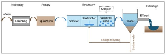
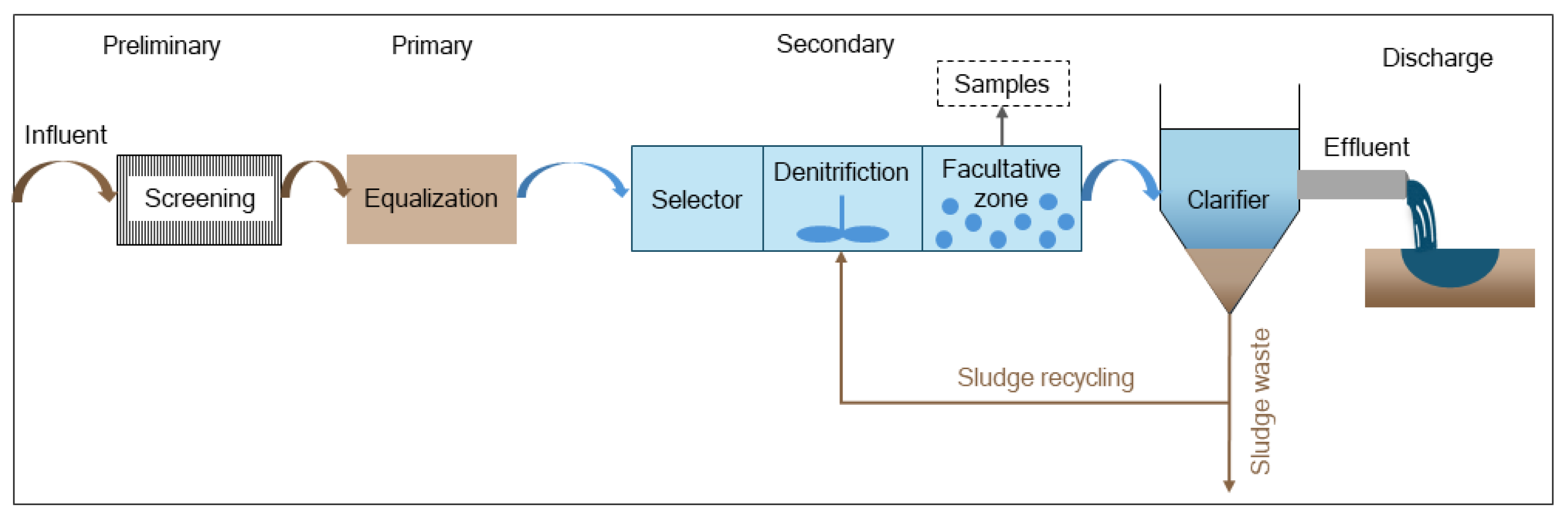
The treatment process at the SWWTP begins with a preliminary screening stage, followed by primary treatment in an equalization tank, and secondary treatment, which involves an activated sludge tank and a settling tank. The activated sludge tank is divided into three distinct zones: the selector, anoxic (for denitrification), and facultative zones, with the aeration volume in the facultative zone ranging from 0 to 3500 ${\displaystyle \frac{{\mathrm{Nm}}^3}{\mathrm{h}}}$. Additionally, the plant features a 2500 m³ equalization tank and a 6700 m³ sludge tank, maintaining a sludge age of 3 to 4 weeks. After treatment, the effluent is released into the Eems River through the Zeehavenkanaal, ultimately flowing into the Wadden Sea [28,29]. A schematic representation of the treatment process is provided in Figure 1.

Figure 1. Schematic representation of the treatment process at the Oosterhorn saline wastewater treatment plant, showing a preliminary treatment step based on screens, a primary treatment step based on an equalization tank, and a secondary treatment step based on an activated sludge tank and a settling tank with sludge recycling. No tertiary treatment is applied; after secondary clarification, the treated effluent is discharged directly to the receiving river (modified from [26]).

The dataset from this previously published sampling campaign spans a duration of two years and four months, with samples collected from 2014 to 2017, specifically targeting the facultative zone of the activated sludge process at the SWWTP. Samples were collected 2–4 weeks apart. A total of 32 activated sludge samples were sequenced. Following metatranscriptome sequencing, these 32 samples underwent analysis using a bioinformatics pipeline to characterize the metabolically active community and their functional transcripts. Comprehensive methodologies for producing the abundance data for the activated sludge microbiome are published in a scientific data paper [26]. Furthermore, this genetic dataset is enriched by various physical, chemical, and biological measurements taken at multiple locations within the SWWTP, thus offering a multi-faceted perspective of the treatment process [30].

2.2. Diversity-Informed Valuation of Ecosystem Functioning

To address the challenges associated with the curse of dimensionality in meta’omics data, we employed Diversity-Informed Valuation of Ecosystem Functioning (DIVE) [31]. DIVE is an algorithmic exploratory framework that links microbiome structure to ecosystem functioning through discrete correlation analysis when samples are unevenly distributed or cross correlation analysis when the samples are evenly distributed, guided by biodiversity-ecosystem functioning (BEF) theory. This deductive research approach was applied to the activated sludge process at the Oosterhorn saline wastewater treatment plant (SWWTP) to identify which microbiome structure, based on functional transcripts abundance data, was most strongly associated with removal performance.

The findings demonstrated that a microbiome characterized by high functional diversity and evenness positively correlated with removal efficiency [31]. Building on these findings, we extended the application of DIVE to determine which process parameters within the SWWTP are most influential in promoting functional diversity in the activated sludge microbiome. The (non-rarefied) Gini-Simpson diversity index of the microbiome was utilized as the response variable, serving as an integrative metric to quantify community diversity. Its values complemented the broader characterization of the microbiome as functionally rich, with abundances distributed relatively evenly among functional features.

2.3. Set of Features

To identify the process parameters that are most predictive of microbiome diversity in the activated sludge process, we analyzed a range of variables, including process control, influent water quality, and sludge quality, which may explain shifts in the microbiome. Table 1 enlists all process parameters used as explanatory variables for the functional diversity in the activated sludge microbiome.

Table 1. Process parameters analyzed for feature importance in predicting activated sludge functional gene diversity.

Acronyms	Measure	Units
BOD5	Biological Oxygen Demand after 5 days	mg_O2/L
Cl	Chlorine	mg/L
COD	Chemical Oxygen Demand	mg_O2/L
EC	Electrical Conductivity	mS/m
K	Potassium	mg/L
N	Total Nitrogen	mg_N/L
Na	Sodium	mg/L
${\mathrm{NH}}_4^{+}$	Ammonium	mg_N/L
Nkj	Total Kjeldahl Nitrogen (TKN)	mg_N/L
${\mathrm{NO}}_2^{-}$	Nitrite	mg_N/L
NO3-	Nitrate	mg_N/L
pH	pH	-
PO4	Phosphate in terms of phosphorus (P) content	mg_P/L
PO4o_P	Orthophosphate Phosphate in terms of phosphorus (P) content	mg_P/L
PO4o	Orthophosphate Phosphate as a whole compound	mg/L
SO4	Sulphate	μg/L
TOD	Total Oxygen Demand	mg_O2/L
TSS	Total suspended solids	mg/L
Temperature	Average temperature	°C
Total_P	Total phosphorus in the inflow stream	kg/day
Sludge_load	Sludge load	kg_COD/kg_DW/day
Glycerol	Glycerol load	kg
Methanol	Methanol load	kg
Return_sludge	Flow rate of the return sludge stream	m3/h
Vol_aeration	Volume of aeration	Nm3/h
Inflow	Inflow	m3/h
Blowers_capacity	Operational load of blowers based on their maximum capacity	%
DW_AT	Dry weight of the activated sludge in the tank; also known as: mixed liquor suspended solids (MLSS)	g/L

2.4. Feature Importance Analysis

To investigate the relationship between process data and functional diversity within the activated sludge microbiome, we employed an explainable machine learning approach. This methodology is grounded in feature importance analysis, where the operational data from the wastewater treatment plant serves as explanatory variables influencing the functional diversity of the activated sludge microbiome. The pipeline encompasses data preprocessing and feature importance analysis, with preprocessing involving the elimination of collinearity and multicollinearity. The feature importance analysis is executed through recursive feature elimination for feature selection in regression modeling. Each component of this process is elaborated upon in the following sections.

2.4.1. Pearson Correlation Coefficient for Eliminating Collinearity

To assess collinearity and eliminate redundancy, the Pearson correlation coefficient (ρ) was calculated to quantify the linear relationships between pairs of variables. The coefficient ranges from −1 to 1, where a positive value indicates that both variables move in the same direction, a negative value indicates an inverse relationship, and a value of 0 signifies no linear dependence. Values of 1 or −1 denote a perfect linear relationship. Statistically, the Pearson correlation coefficient is essentially the covariance of the two variables divided by the product of their standard deviations [32]. For any given pair of i, j ∈ {1, 2, 3, …, p}, where p is the number of explanatory variables, the Pearson correlation coefficient between two independent variables x_i and x_j (denoted by ρ(x_i,x_j)) is defined by:

$$\rho \left(x_i,x_j\right)={\displaystyle \frac{{\displaystyle {\sum }_{k=1}^n}\left(x_{i,k}-{\overline{x}}_i\right)\left(x_{j,k}-{\overline{x}}_j\right)}{\sqrt{{\displaystyle {\sum }_{k=1}^n}{\left(x_{i,k}-{\overline{x}}_i\right)}^2}·\sqrt{{\displaystyle {\sum }_{k=1}^n}{\left(x_{j,k}-{\overline{x}}_j\right)}^2}}},$$

(1)

where n is the sample size, p is the number of explanatory variables in the dataset, x_i,k and x_j,k denote the k-th observation of the variables x_i and x_j, respectively and ${\overline{x}}_i={\displaystyle \frac{1}{n}}{\displaystyle {\sum }_{k=1}^n}{x}_{i,k}$ is the sample mean of x_i; and analogously for ${\overline{x}}_j$. Based on these Pearson correlation coefficients ρ(x_i,x_j) for all i, j = 1, 2, 3, …, p, a Pearson correlation coefficient matrix r is given by:

$$\mathit{r}=\left[\begin{array}{ccc}\begin{array}{cc}\mathbf{1}& \rho (x_1,x_2)\\ \rho (x_2,x_1)& \mathbf{1}\end{array}& \dots & \begin{array}{cc}\rho (x_1,x_{p-1})& \rho (x_1,x_p)\\ \rho (x_2,x_{p-1})& \rho (x_2,x_p)\end{array}\\ ⋮& \ddots & ⋮\\ \begin{array}{cc}\rho (x_{p-1},x_1)& \rho (x_{p-1},x_2)\\ \rho (x_p,x_1)& \rho (x_p,x_2)\end{array}& \dots & \begin{array}{cc}\mathbf{1}& \rho (x_{p-1},x_p)\\ \rho (x_p,x_{p-1})& \mathbf{1}\end{array}\end{array}\right].$$

(2)

The matrix r is symmetric because ρ(x_i,x_j) = ρ(x_j,x_i) and has ones on the diagonal, as each variable is perfectly correlated with itself.

Variables exhibiting strong pairwise correlations (|r| > 0.7) were considered potentially redundant. For correlated variable pairs, the final selection was based on process interpretation and operational relevance, retaining the variable that provided the most direct and actionable representation of the underlying process while excluding redundant predictors from subsequent feature selection.

2.4.2. Variance Inflation Factor for Eliminating Multi-Collinearity

Multi-collinearity occurs when two or more independent variables in a multiple regression are highly linearly related, impacting the reliability of coefficient estimates and interpretability. Statistically, multi-collinearity inflates the standard errors of the estimates of the regression coefficients, often reducing the statistical significance of individual predictors and causing instability in coefficient estimates. Computationally, multi-collinearity can lead to numerical instability, as small changes in data may lead to large fluctuations in coefficient estimates.

The Variance Inflation Factor (VIF) quantifies the inflation in variance of a regression coefficient estimate due to multicollinearity [33]. For each independent variable X_i, VIF is computed by regressing X_i on all other explanatory variables, as shown in Equation (3). The coefficient of determination $R_i^2$ from this regression is then used in Equation (5) to calculate VIF, which expresses the factor by which the variance of X_i ‘s coefficient estimate is inflated due to collinearity with other predictors.

$$X_i={\alpha }_0+\sum _{j\ne i}{\alpha }_j{X}_j+e_i\hspace{1em}\hspace{1em}\hspace{1em}\hspace{1em}\hspace{1em}\hspace{1em}\forall i\in \left\{1,2,3,\dots ,p\right\},$$

(3)

where α₀ is a coefficient, x_i is an independent variable, e_i is an error term and i is the index, and p is the number of explanatory variables in the dataset.

$$R_i^2=1-{\displaystyle \frac{\mathit{RSS}}{\mathit{TSS}}}=1-{\displaystyle \frac{{\displaystyle {\sum }_{j=1}^n}{\left(x_{i,j}-{\widehat{x}}_i\right)}^2}{{\displaystyle {\sum }_{j=1}^n}{\left(x_{i,j}-{\overline{x}}_i\right)}^2}}\hspace{1em}\hspace{1em}\hspace{1em}\forall i\in \left\{1,2,3,\dots ,p\right\},$$

(4)

where $R_i^2$ is the coefficient of determination for regression of the i-th independent variable (X_i) on the remaining variables (from Equation (3)), RSS is the residual sum of squares for the i-th independent variable, TSS is the total sum of squares for the i-th independent variable, x_i,j is an observation of X_i, ${\overline{x}}_i={\displaystyle \frac{1}{n}}{\displaystyle {\sum }_{j=1}^n}{x}_{i,j}$ is the mean value of variable x_i (sample mean), ${\widehat{x}}_i$ is the estimated/fitted value of the independent variable x_i, p is the number of explanatory variables in the dataset, and n is the sample size.

$${\mathit{VIF}}_i={\displaystyle \frac{1}{1-R_i^2}}\hspace{1em}\hspace{1em}\hspace{1em}\hspace{1em}\hspace{1em}\hspace{1em}\forall i\in \left\{1,2,3,\dots ,p\right\}.$$

(5)

A VIF of 1 indicates no multicollinearity, as the variable is uncorrelated with others. A VIF between 1 and 5 suggests moderate multicollinearity, while a VIF greater than 5 often indicates high multicollinearity, warranting closer examination. VIF_i > 5 is commonly used as a cutoff to exclude the respective variable X_i.

Here, multi-collinearity was eliminated by eliminating explanatory variables with missing data-points in the composite dataset and by reaching a resulting mean VIF less than 2.5 [34].

2.4.3. Recursive Feature Elimination for Feature Selection in Regression Modeling

Recursive Feature Elimination (RFE) is a powerful wrapper algorithm utilized for feature selection in regression modeling [35]. RFE can leverage various machine learning models as base estimators, allowing for the incorporation of hyperparameters throughout the feature selection process. During this iterative selection, the base model functions as an external estimator that assigns importance scores to features.

RFE employs a backward selection methodology, initially fitting the model to the entire dataset to compute the importance scores of each feature. It then recursively removes the least important predictors, refining the feature set while continuously assessing the model’s performance. This process effectively identifies the optimal subset of features that contribute most significantly to predicting the target variable based on their importance rankings.

While RFE evaluates all possible feature combinations in a greedy manner, it is essential to note that this approach may lead to overfitting and reduced generalizability [36]. Nevertheless, RFE remains a robust feature selection technique, particularly in regression modeling, model individualization [37], and reverse engineering applications [38]. In this study, RFE is employed as a greedy search method to identify key features within a biological system, focusing on significant explanatory variables for our machine learning model.

2.4.4. Regression Trees in Bagged Trees and Random Forests

Decision tree methods are supervised learning approaches applicable to both classification and regression tasks. In the context of regression, these trees predict the value of a target variable based on multiple input features [39]. The dataset D for regression trees is structured as follows:

D = (X₁, X₂, X₃, … , X_P, Y).

(6)

Here, Y is the dependent variable (target), and X₁, X₂, X₃, … , X_P are the independent variables (features).

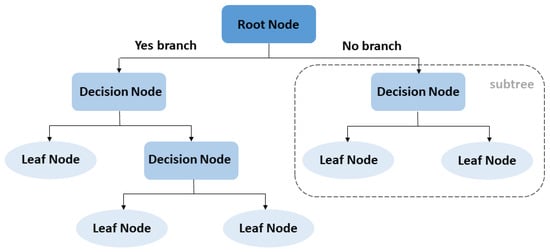
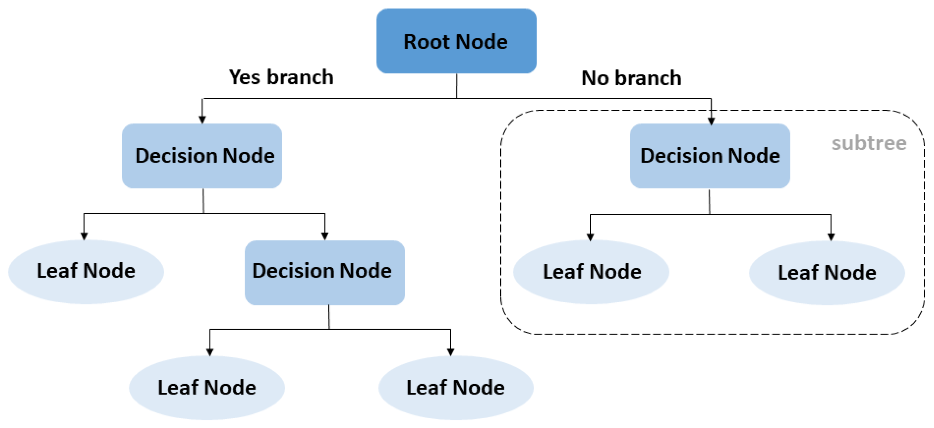
Decision trees visually map features to target values, consisting of two primary phases: tree growth and pruning as illustrated in Figure 2. During the tree growth phase, the predictor space is segmented, and target values are estimated using the mean of training observations within each segment. The resulting tree structure can be visualized as an upside-down tree, with the root node at the top and terminal nodes at the bottom.

Figure 2. Simplified conceptual diagram of regression trees.

The objective of a regression tree is to construct a model f(x) that fits the dataset D while minimizing a loss function. For instance, when a regression tree divides the input space X into J regions $R_1{,R_2,\dots ,R}_J$, the aim is to minimize the residual sum of squares (RSS):

$$\min {\displaystyle \sum _{j=1}^J}\sum _{{{i:x}_i\in R}_j}{\left({y_i-\widehat{y}}_{R_j}\right)}^2,$$

(7)

where ${\widehat{y}}_{R_j}$ is the mean response for training observations within the j-th region:

$${\widehat{y}}_{R_j}=\mathrm{avg}\left(y_i|x_i\in R_j\right).$$

(8)

Recursive binary splitting employs a top-down greedy approach to evaluate all predictors X₁, X₂, X₃, … ,X_P and their potential cut points s, constructing a decision tree that minimizes RSS.

To mitigate the risk of overfitting to the training data, cost-complexity pruning is applied. Initially, the tree is allowed to grow without restrictions using the training data. The resulting tree T₀ is then pruned, grouping regions to reduce variance while introducing a controlled bias. Cost-complexity pruning addresses the overfitting observed in the training set by correcting for it, ensuring the decision tree’s generalizability through the removal of certain branches. The choice of subtree that results in the minimum penalized error (SSE_λ) is determined by estimating penalized error for subtrees via cross-validation, represented as:

$${\mathit{SSE}}_{\mathrm{\lambda }}={\displaystyle \sum _{j=1}^{\left|T\right|}}\sum _{{{i:x}_i\in R}_j}{\left({y_i-\widehat{y}}_{R_j}\right)}^2+\mathrm{\lambda }\left|T\right|.$$

(9)

In this equation, λ is a non-negative tuning parameter that balances the trade-off between tree complexity and overfitting, while |T| signifies the number of terminal nodes in the respective tree or subtree.

The resulting regression tree model is expressed as:

$$f\left(x\right)={\displaystyle \sum _{j=1}^J}{\widehat{y}}_{R_j}\mathbb{l}\left(x\in R_j\right),$$

(10)

where $R_1{,R_2,\dots ,R}_J$ denote the partitions of the feature space corresponding to the input space X₁, X₂, X₃, …, X_P.

While decision trees offer simplicity and interpretability, they may also suffer from high variance, which can negatively impact prediction accuracy. To enhance predictive performance, ensemble methods such as bagged trees and random forests are employed.

2.4.5. Bagged Trees

Bagging, or bootstrap aggregating, involves generating B distinct tree models using B bootstrapped training sets, sampled with replacement from the original dataset [40]. Each tree is grown without pruning, resulting in high variance and low bias. The final prediction is obtained by averaging the outputs of these trees:

$${\widehat{f}}_{\mathit{bag}}\left(x\right)={\displaystyle \frac{1}{B}}{\displaystyle \sum _{b=1}^B}{f}^b\left(x\right),$$

(11)

where B represents the number of bootstrapped training datasets, f^b(x) is the individual regression tree model trained on the b-th bootstrapped dataset, and f^b(x) is the resulting bagged tree from averaging all individual regression trees.

2.4.6. Random Forest

The random forest algorithm extends the bagging approach by randomly selecting subsets of features at each split within the trees, further reducing prediction variance through decorrelation of the trees. By considering approximately $m\approx \sqrt{p}$ predictors at each split, random forests enhance the diversity of tree structures [41].

While both bagged trees and random forests improve predictive performance, they may compromise model interpretability. However, variable importance can still be assessed by averaging the reductions in RSS attributable to splits across all trees.

2.4.7. Performance Measurement: Root Mean Square Error (RMSE)

To evaluate the predictive performance of the proposed model, we calculate the root mean square error (RMSE) as follows [42]:

$$\mathit{RMSE}=\sqrt{{\displaystyle \frac{1}{m}}{\displaystyle \sum _{i=1}^m}{(y_i-{\widehat{y}}_i)}^2}.$$

(12)

In this equation, m denotes the number of predictions, y_i represents the actual target value, and $\widehat{y}$ is the predicted value.

The relevant data and the algorithmic implementation for the machine learning pipeline are available through a publicly accessible repository on GitHub [43].

3. Results and Discussion

Prior to data preprocessing, an automated exploratory data analysis (EDA) report was generated for the raw dataset (Supplementary Material Files S1–S4). The complete EDA reports are provided in the Supplementary Material. These reports include descriptive summary statistics (e.g., the number of observations and variables, variable types, missing and complete observations, and memory allocation), providing an overview of dataset completeness and structure. They also summarize the proportions of continuous and discrete variables and quantify missing data, facilitating the identification of potential data quality issues. Graphical visualizations include data structure plots to assess the organization of observations, missing data profiles for each process parameter to identify patterns of missingness, univariate histograms to examine variable distributions, and quantile–quantile (Q–Q) plots to evaluate departures from normality and detect potential outliers. In addition, principal component analysis (PCA) is included to summarize the multivariate structure of the dataset, including the proportion of variance explained by each principal component and the contribution of individual process parameters to each component. Together, these analyses provide a comprehensive assessment of data quality, distributional characteristics, missing data patterns, and multivariate relationships before subsequent preprocessing and machine learning analyses.

Exploratory data analysis (EDA) revealed significant data misalignment and disparity, stemming from inconsistent sampling frequencies across datasets: hourly for online measurements, daily for methanol loading and glycerol loading, and sporadic intervals for influent water quality, all of which were misaligned with microbiome sampling times. Hence, data pre-processing was conducted prior to data harmonization in order to maximize the informative content of the dataset while eliminating redundancy.

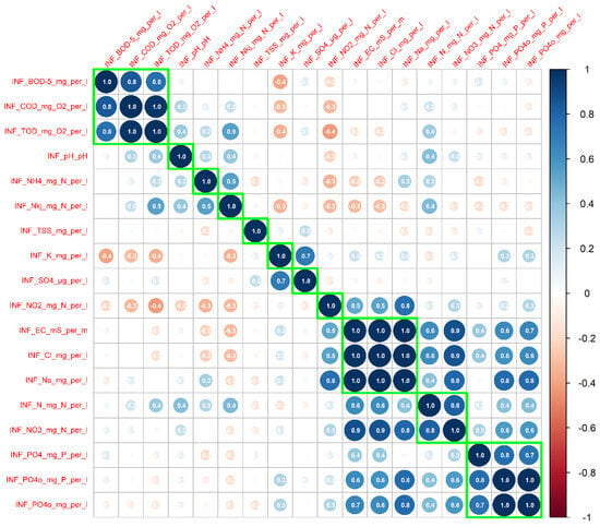
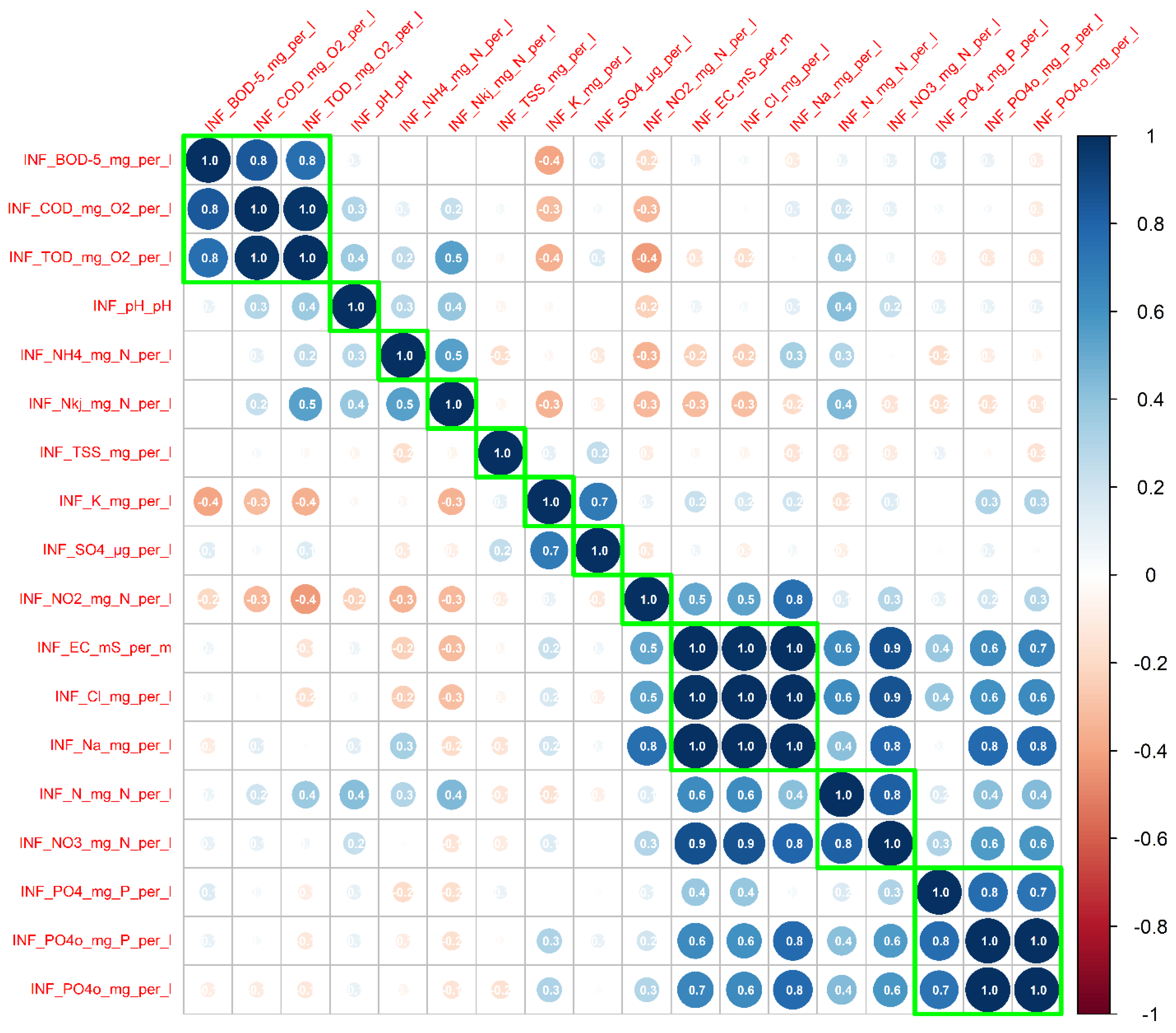
To maximize the knowledge potential from the original dataset, we conducted a collinearity analysis to eliminate redundant parameters prior to integrating the original dataset into a composite dataset aligned with microbiome samples. As illustrated in Figure 3, Pearson correlation analysis primarily clusters four groups of parameters. Notably, strong correlations are observed among total oxygen demand (TOD), biological oxygen demand (BOD), and chemical oxygen demand (COD), which aligns with established definitions and underscores their collective dependence on organic matter for measurement. Additionally, the analysis reveals a strong correlation between electrical conductivity (EC) and the concentrations of sodium (Na) and chloride (Cl) ions in solution, attributable to the fundamental properties of ionic solutions and the behavior of dissolved salts.

Figure 3. Pearson correlation heatmap showing pairwise relationships among influent water-quality parameters based on 2520 observations. Green boxes delineate clusters of strongly correlated variables. Circle size represents the absolute magnitude of the Pearson correlation coefficient, while circle color indicates its sign and value according to the color scale.

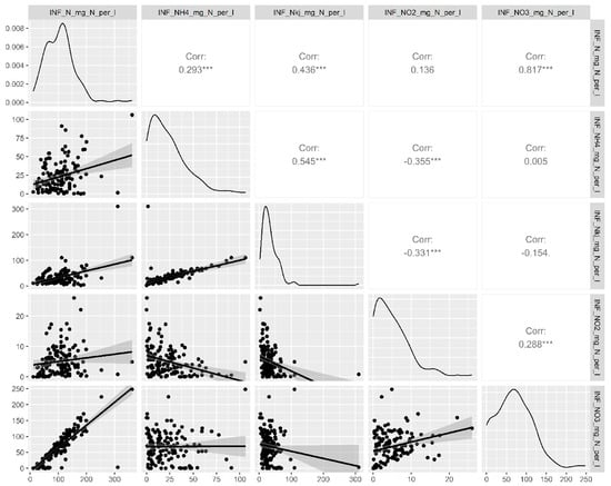
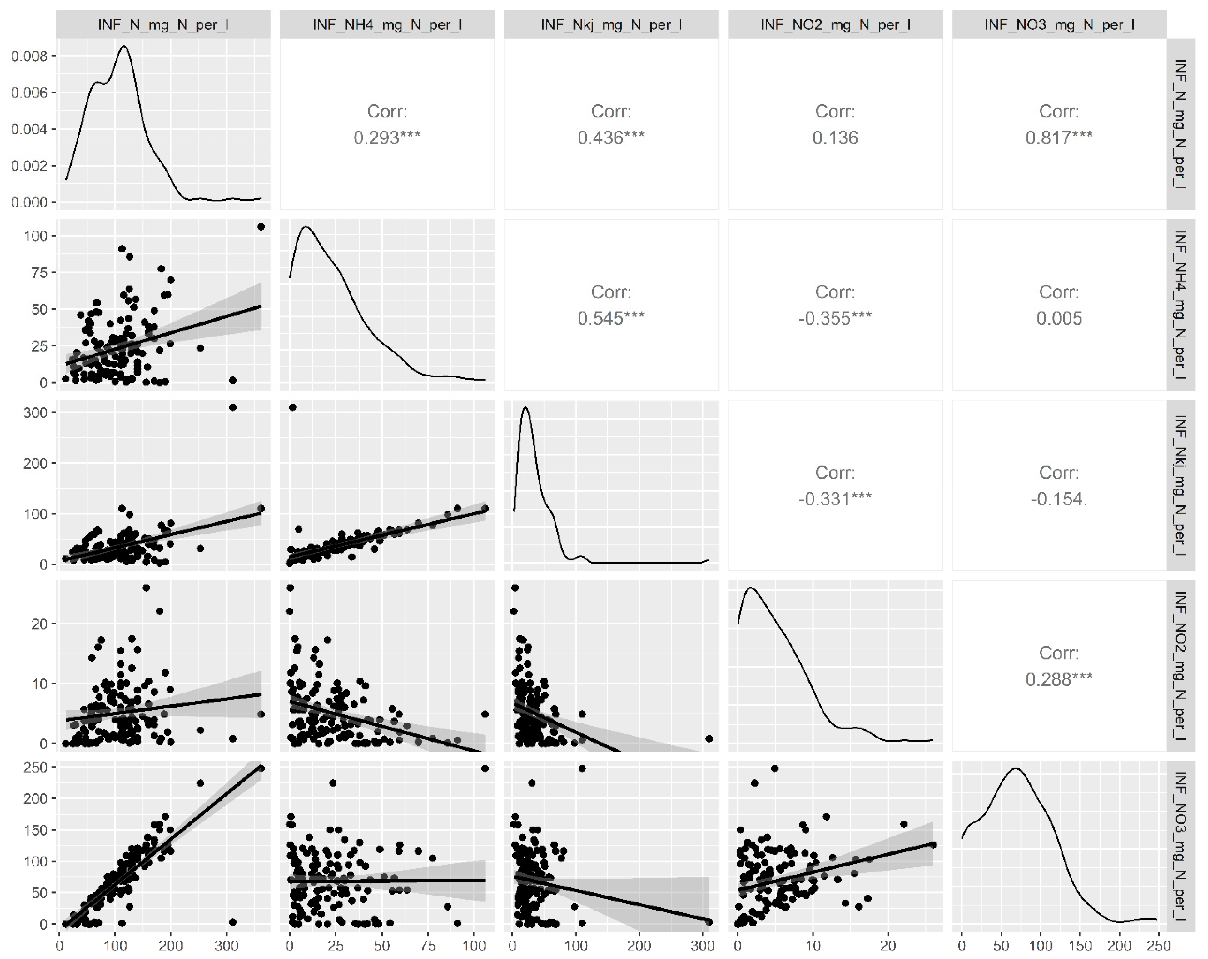
Taking into account physical principles, we observed limited collinearity among various nitrogen forms using Pearson correlation analysis. To address the limitations of this method for collinearity elimination, we employed multiple data visualization techniques during the data pre-processing phase. Specifically, pair plots were utilized to reveal relationships among nitrogen speciation that were missed by Pearson correlation alone. As demonstrated in Figure 4, a strong relationship between ammonium (NH₄) and Kjeldahl nitrogen (Nkj) became evident following visual inspection of the data, despite being obscured in the Pearson correlation analysis by the influence of a single extreme outlier. Recognizing this effect enabled the underlying collinearity between the two variables to be appropriately considered during variable selection. This example illustrates the value of combining statistical analyses with exploratory data visualization and domain knowledge when interpreting relationships among explanatory variables.

Figure 4. Pairs plot illustrating relationships among nitrogen forms. Upper-right panels report Pearson correlation coefficients; *** indicates (p < 0.001). Lower-left panels show pairwise scatterplots with fitted trend lines and shaded confidence bands. Diagonal panels show the distribution of each variable.

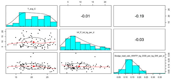
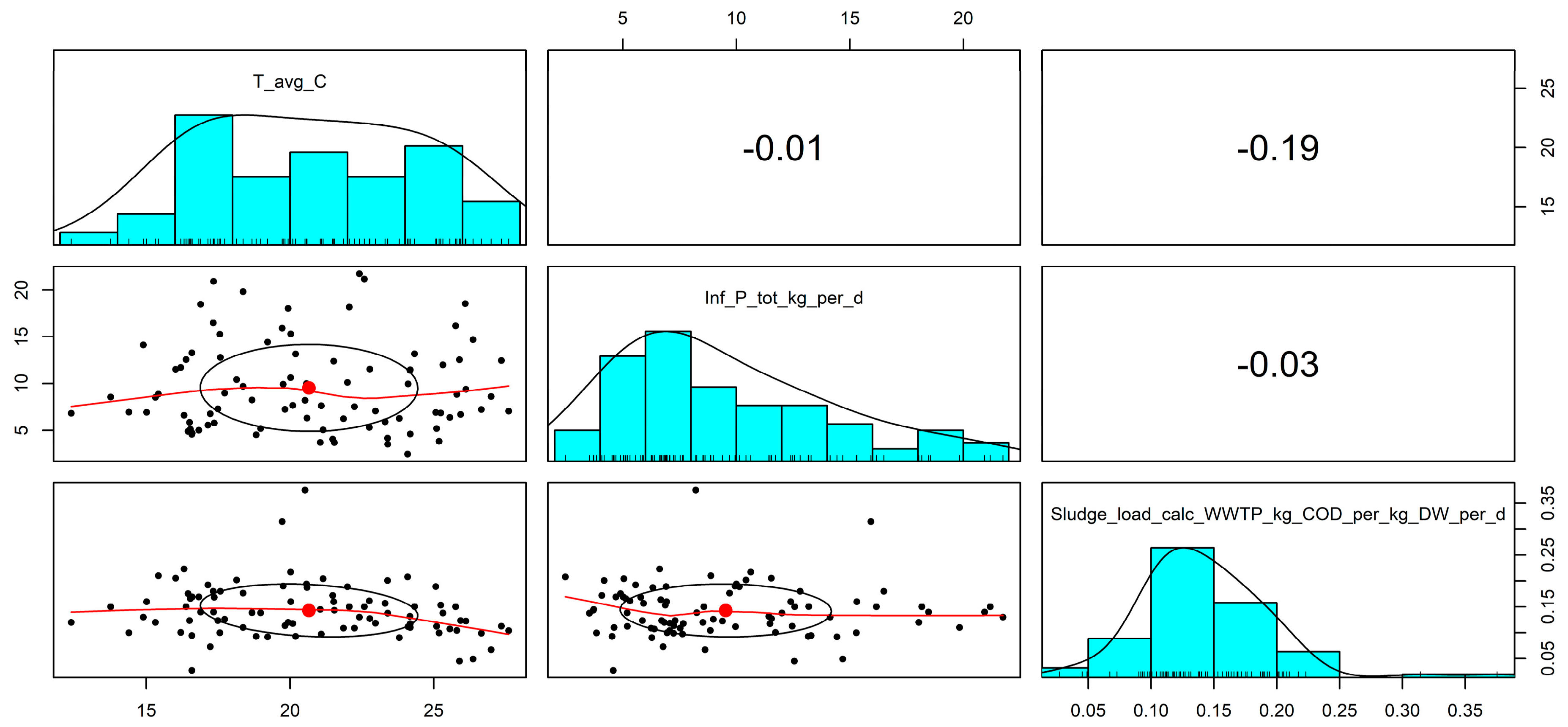
Figure 5 presents a pairs plot illustrating the relationships among the operational and environmental variables retained for further analysis, including temperature, total phosphorus in the inflow, and sludge load. Visual inspection of the pairwise relationships, together with the corresponding correlation coefficients, indicated that no strong collinearity was present among these variables. Consequently, all variables were retained for the subsequent recursive feature elimination analysis.

Figure 5. Pairs plot illustrating relationships among temperature, influent total phosphorus, and sludge load based on 445 observations. Upper-right panels report Pearson correlation coefficients. Lower-left panels show pairwise scatterplots with red fitted trend lines, black ellipses summarizing the bivariate spread, and red dots indicating the centers of the distributions. Diagonal panels display histograms with overlaid density curves. Pairwise correlations were weak, and all three predictors were retained for subsequent recursive feature elimination.

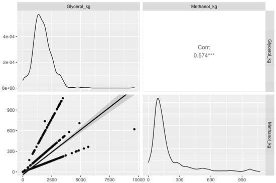
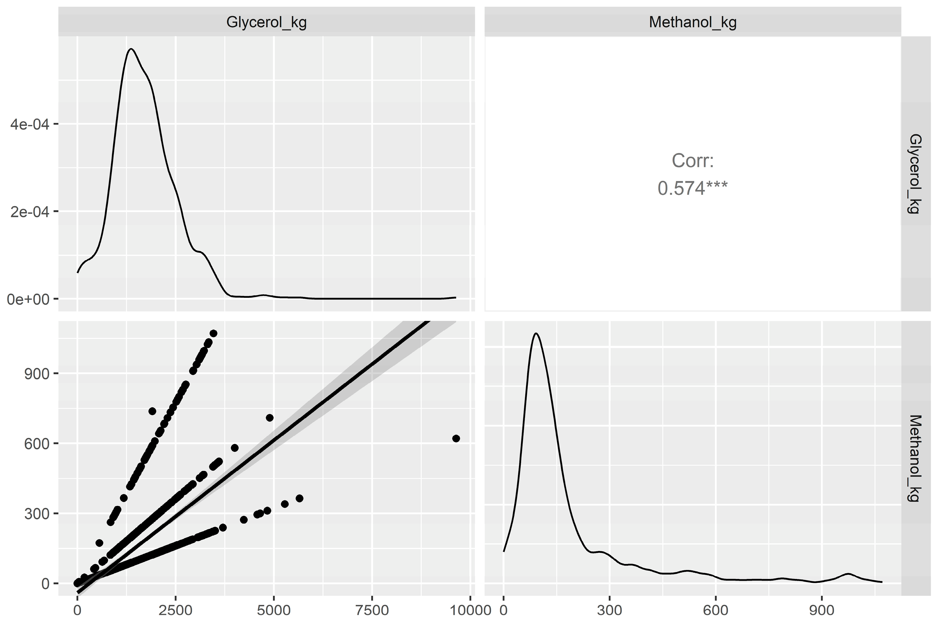
Figure 6 presents a pairs plot illustrating the relationship between methanol load and glycerol load. Although the Pearson correlation coefficient indicated only a weak overall linear association, the scatterplot revealed three distinct linear trends originating near the origin and characterized by different slopes. This pattern indicates the presence of multiple proportional relationships between the two carbon-source loads rather than a single global linear relationship. Such structure may reflect the facultative operation of the treatment process, in which different operational modes or treatment objectives, including changes in denitrification requirements, result in different methanol-to-glycerol dosing ratios. Accordingly, the low overall Pearson correlation should not be interpreted as complete independence between the variables, but as the combined effect of several operationally distinct relationships.

Figure 6. Pairs plot illustrating the relationship between methanol and glycerol loads in the wastewater treatment plant based on 1744 observations. The upper-right panel reports the Pearson correlation coefficient (*** denotes p < 0.001). The lower-left panel shows the paired observations, a fitted trend line, and a shaded band representing uncertainty around the fitted trend. Although the Pearson correlation coefficient indicates a weak overall linear association, the scatterplot reveals three distinct linear trends originating near the origin, suggesting that the relationship may vary under different operational modes or treatment objectives within the wastewater treatment process.

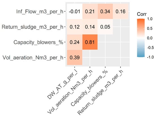
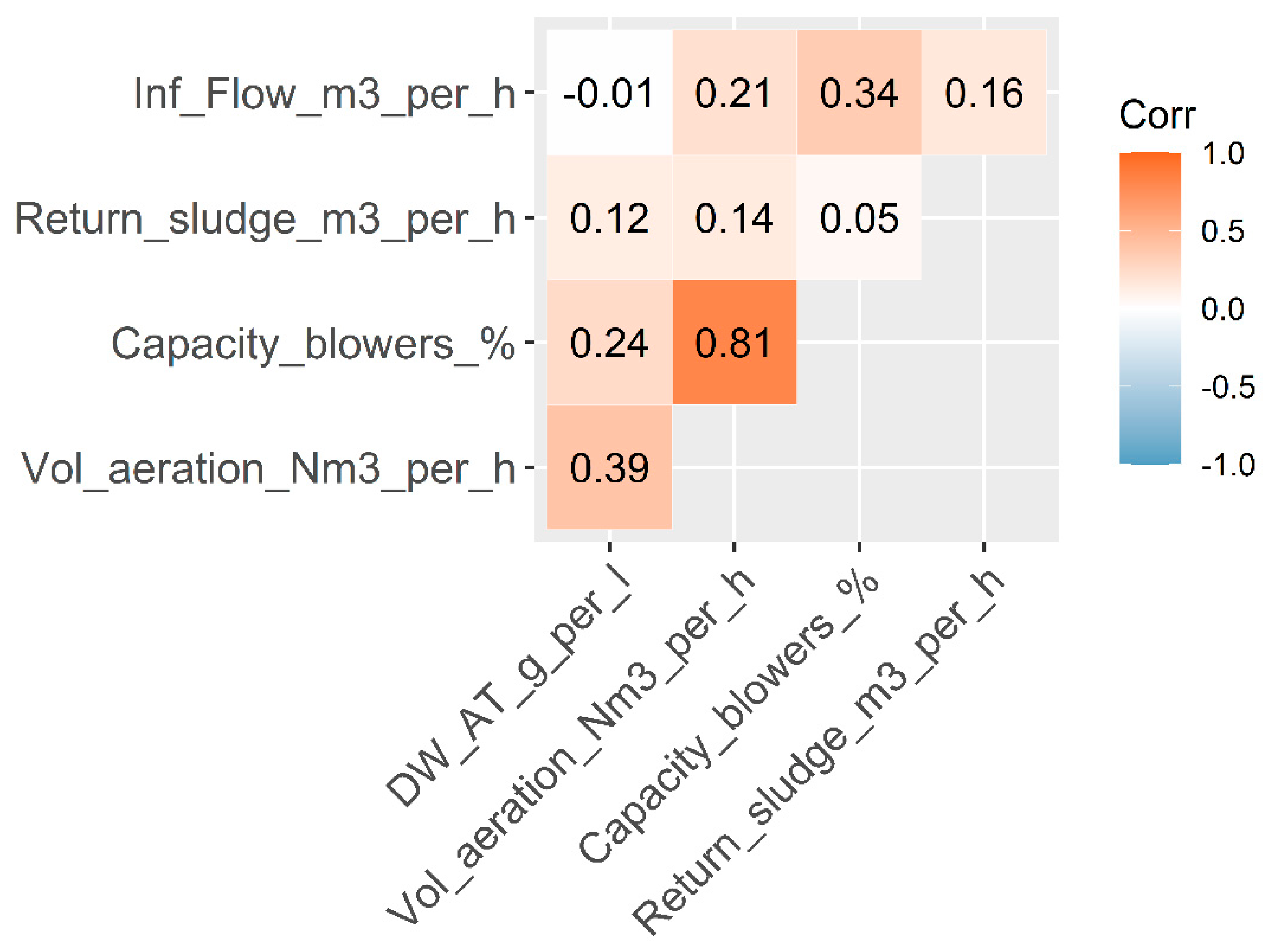
Figure 7 presents a correlation heatmap of the operational variables, including the operational load of blowers based on their maximum capacity, volume of aeration, mixed liquor suspended solids (MLSS; dry weight of activated sludge in the aeration tank), and the return sludge flow rate. A strong correlation was observed between blower operational load and aeration volume, indicating that both variables describe closely related aspects of the aeration process. To reduce collinearity, blower operational load was retained for subsequent analyses because it represents a directly controllable operational parameter that can be adjusted by plant operators to optimize process performance.

Figure 7. Correlation heatmap illustrating the relationships among the operational variables: blower operational load based on maximum capacity, aeration volume, mixed liquor suspended solids (MLSS), and return sludge flow rate based on 259,200 observations. Color intensity represents the strength and direction of the Pearson correlation coefficient. A strong positive correlation was observed between blower operational load and aeration volume, whereas the remaining variables exhibited weak to moderate correlations. Blower operational load was retained for subsequent analyses because it represents a directly controllable operational parameter that can be adjusted to optimize process performance.

Following the collinearity analysis, data harmonization was performed to reconcile the differences between the process data and the microbiome samples. The datasets used in this study were collected at different temporal resolutions, reflecting the practical constraints associated with routine wastewater treatment plant monitoring and metatranscriptomic analyses. Operational process parameters, such as blower load, were continuously monitored online and recorded hourly, while methanol and glycerol loading were recorded daily. Influent water quality parameters were measured at irregular intervals. In contrast, metatranscriptomic data required activated sludge sampling, RNA extraction, sequencing, and bioinformatic analysis, making frequent sampling impractical because of the associated cost and analytical complexity. Consequently, microbiome samples were collected at intervals of several weeks.

To integrate measurements collected at different frequencies, available process measurements were averaged within the calendar week corresponding to each activated-sludge sample. This provided a common temporal reference for exploring associations between functional diversity and weekly operational conditions. However, the sampling design did not consistently provide environmental and process measurements coinciding with microbial collection. Weekly averages may therefore obscure short-lived disturbances and differ from conditions at the time of sampling, particularly where transcriptional responses occur over shorter timescales. They may also include observations collected after the microbial sample and consequently cannot establish exposure precedence. The resulting associations are interpreted as relationships with weekly operational context rather than immediate microbial responses, precise response delays, or causal effects. This limitation constrains temporal interpretation but does not preclude descriptive exploration of the available observations.

The integrated dataset was then assessed for multicollinearity prior to the feature selection phase. To mitigate multicollinearity which is characterized by significant linear relationships among explanatory variables in multiple regression, we removed variables with missing data points and ensured that the mean Variance Inflation Factor (VIF) remained below 2.5. This approach effectively prevents inflated standard errors and preserves the statistical significance of independent variables.

Following data preprocessing, which included feature selection after collinearity analysis, data harmonization, and a second feature selection step following multicollinearity analysis, an analysis-ready dataset was generated for subsequent machine learning analyses. The resulting composite dataset and its respect EDA report are attached as Supplementary Material Files S5 and S6. This machine learning-ready dataset comprised the subset of environmental and operational variables considered most suitable for predictive modeling after the removal of redundant and highly correlated features. The selected predictor variables are summarized in Table 2. These variables served as the input features for the recursive feature elimination and Random Forest modeling procedures described in the subsequent sections.

Table 2. Predictor variables retained in the analysis-ready dataset after collinearity assessment, data harmonization, and multicollinearity-based feature selection. These variables were used as input features for the recursive feature elimination and Random Forest analyses.

Acronyms	Measure	Units
Cl	Chlorine	mg/L
COD	Chemical Oxygen Demand	mg_O2/L
N	Total Nitrogen	mg_N/L
Nkj	Total Kjeldahl Nitrogen (TKN)	mg_N/L
PO4o	Orthophosphate Phosphate in terms of phosphorus (P) content	mg_P/L
SO4	Sulphate	μg/L
TSS	Total suspended solids	mg/L
Temperature	Average temperature	°C
Glycerol	Glycerol load	kg
Return_sludge	Flow rate of the return sludge stream	m3/h
Inflow	Inflow	m3/h
Blowers_capacity	Operational load of blowers based on their maximum capacity	%
DW_AT	Dry weight of the activated sludge in the tank; also known as: mixed liquor suspended solids (MLSS)	g/L

Recursive feature elimination (RFE) was applied to identify a parsimonious subset of predictors associated with functional gene diversity. Random forest regression was selected as the base learner because of its ability to model complex non-linear relationships, its robustness to correlated predictors, and its intrinsic estimation of variable importance. The RFE procedure was implemented using repeated 10-fold cross-validation with five repetitions, resulting in 50 resampling iterations for each candidate feature subset [44].

The random forest model was constructed using 500 trees, a commonly adopted value that provides stable estimates of prediction error and variable importance while maintaining computational efficiency [41]. At each decision node, one predictor was selected as a candidate for splitting. This setting increases diversity among the trees within the ensemble and reduces the likelihood of overfitting by introducing additional stochasticity into the model-building process [41,45].

Repeated cross-validation was used to evaluate both predictive performance and the stability of feature selection. During each repetition, the dataset was partitioned into ten folds, with nine folds used for model training and the remaining fold used for validation. The procedure was repeated until each fold had served once as the validation set, after which a new random partitioning was generated for the next repetition. Consequently, every candidate feature subset was evaluated across 50 independent resampling iterations. This resampling strategy reduces the dependence of the estimated prediction error on a single partition of the data and provides a more robust assessment of model generalizability and feature-selection stability [46,47].

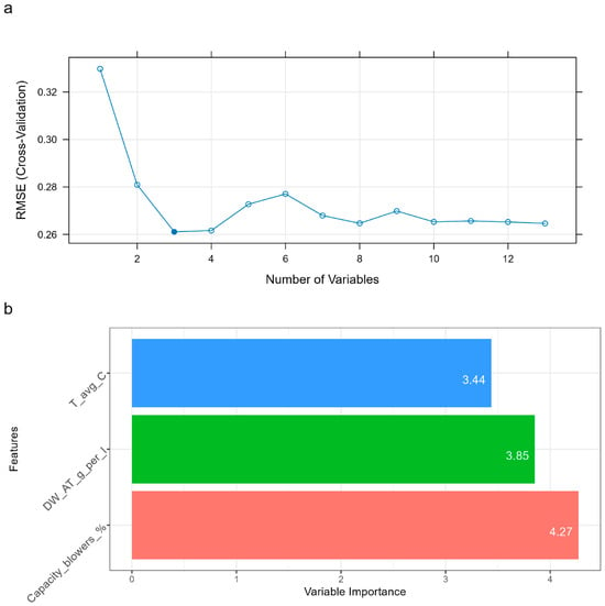
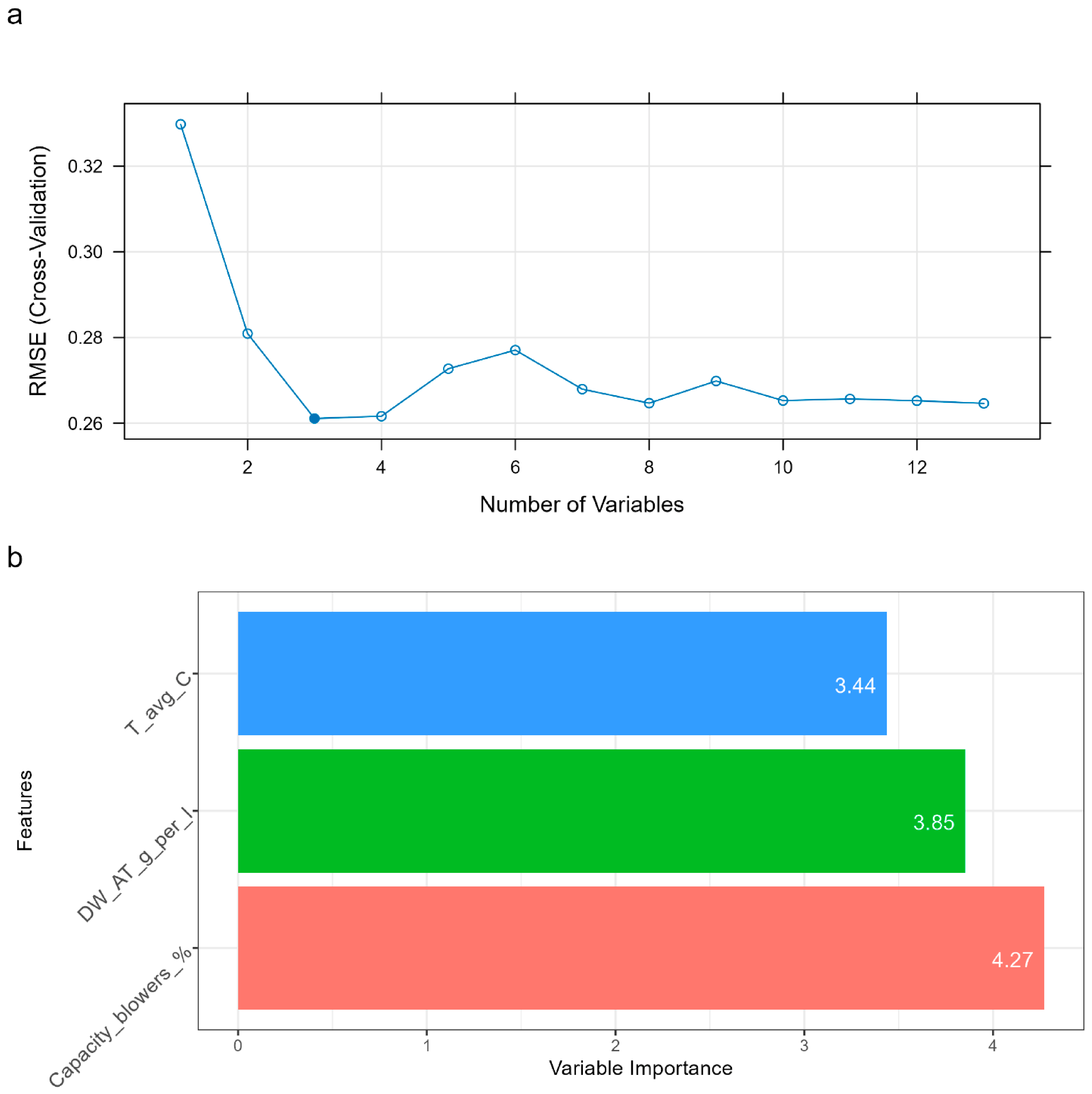
The RFE resampling profile is presented in Figure 8a. The model containing three predictors achieved the lowest mean cross-validated root mean square error (RMSE) among the evaluated feature subsets. However, the reduction in RMSE relative to models containing additional predictors was small. Therefore, the three-feature model was selected as the most parsimonious model achieving the minimum cross-validated prediction error rather than being interpreted as uniquely superior to all larger candidate models.

Figure 8. (a) Mean cross-validated root mean square error (RMSE) as a function of the number of predictors evaluated during recursive feature elimination using random forest regression with 10-fold cross-validation. The filled dot identifies the selected three-predictor model, representing the most parsimonious subset achieving the minimum mean cross-validated prediction error. (b) Permutation-based variable importance from the selected random forest model, expressed as the percentage increase in out-of-bag mean squared error after randomly permuting each predictor. Higher values indicate greater predictive importance within the fitted model. Blower operational load (% of maximum capacity) had the highest importance, followed by activated-sludge dry weight in the aeration tank (DW_AT; also termed mixed liquor suspended solids, MLSS) and temperature (T).

The observed Gini–Simpson diversity index ranged from 0.049 to 0.988 across the 32 samples (mean = 0.604; standard deviation = 0.271). The final three-predictor random forest model produced an out-of-bag RMSE of approximately 0.264 and explained 5.5% of the observed variance. The modest explained variance is not unexpected given the complexity of full-scale activated sludge systems, where functional gene diversity may reflect the combined effects of numerous measured and unmeasured environmental, operational, ecological, and temporal factors. Importantly, the objective of the analysis was not to account for the majority of the total variance, but to determine which measured variables contained the greatest relative predictive information. Within the evaluated predictor set, blower operational load, mixed liquor suspended solids, and temperature formed the most informative and parsimonious subset identified by recursive feature elimination. Thus, the low overall explained variance limits the predictive scope of the model but does not, by itself, invalidate the relative ranking of the predictors.

Figure 8b presents the permutation-based variable importance obtained from the final random forest model. The operational load of the blowers relative to their maximum capacity exhibited the highest permutation importance, followed by mixed liquor suspended solids and temperature. These values indicate the relative contribution of the retained predictors to the predictive signal captured by the model. Accordingly, blower operational load can be interpreted as the highest-ranked predictor among the variables evaluated, although this does not imply that it explains the majority of variation in functional transcripts diversity in the full-scale system.

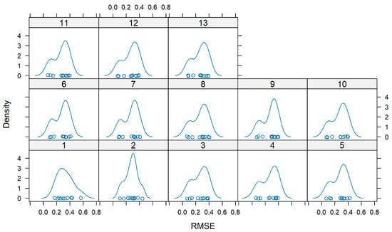
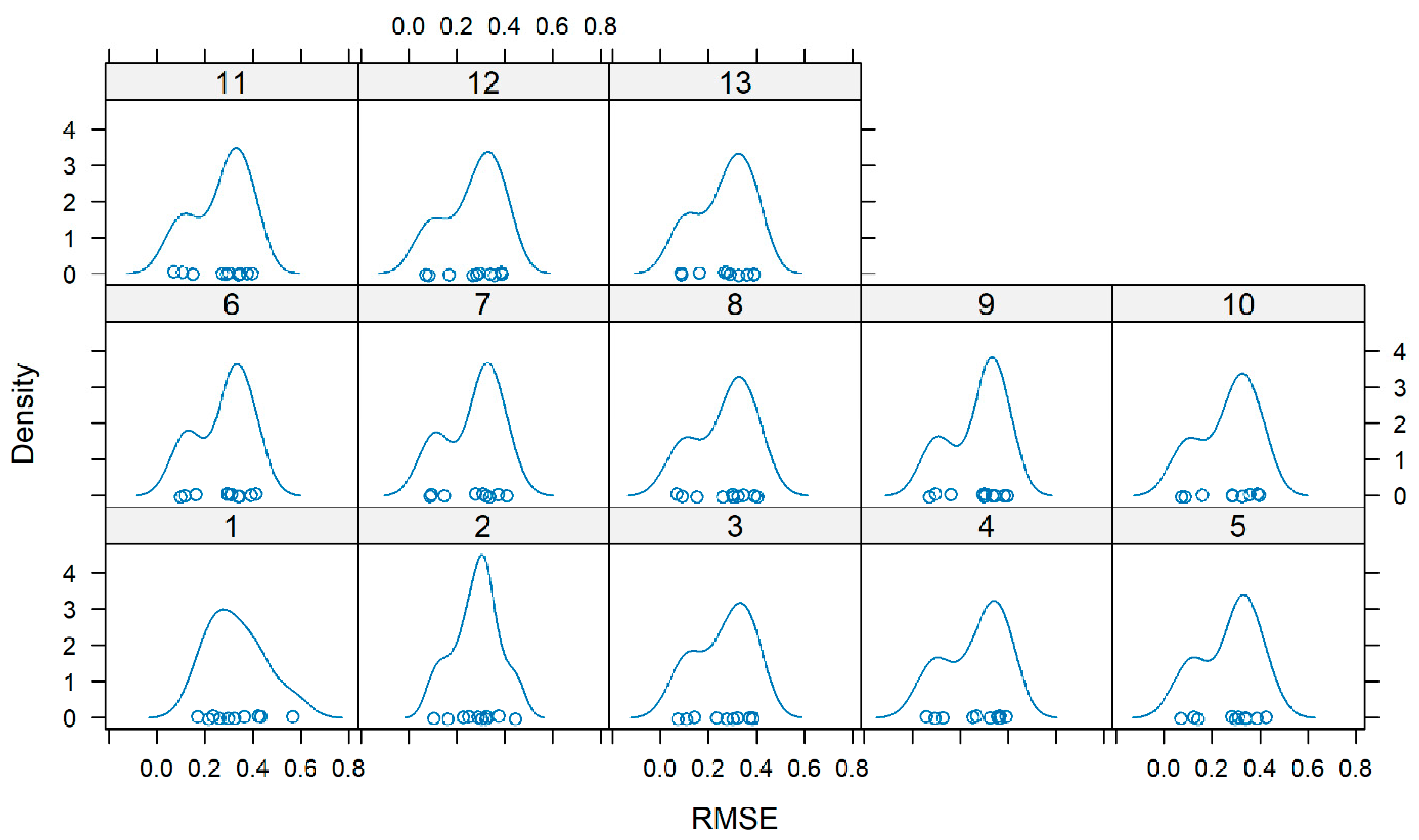
To further evaluate the robustness of the feature-selection procedure, Figure 9 presents the density distributions of the RMSE estimates obtained across all 50 resampling iterations for each candidate feature-subset size. Considerable overlap is observed among the RMSE distributions for models containing three or more predictors, indicating that these models exhibit broadly comparable predictive performance under the applied resampling framework. Although the three-feature model consistently achieved the lowest mean RMSE, the overlap of the distributions indicates that the practical differences in predictive performance among models containing three or more predictors are small. Accordingly, the three-feature model was retained because it achieved the minimum estimated mean cross-validated RMSE while representing the simplest model.

Figure 9. Density distributions of cross-validated root mean square error (RMSE) estimates for Random Forest regression models using different numbers of predictor variables during recursive feature elimination. Each density curve represents the distribution of RMSE values obtained across the cross-validation resamples for a given predictor subset.

To further assess the robustness of the identified predictors, a second RFE analysis was performed using the same composite dataset but with an alternative modelling configuration. In this analysis, bagged trees were used as the base learner and Leave-One-Out Cross-Validation (LOOCV) served as the resampling strategy. Bagged trees employ bootstrap aggregation to reduce prediction variance, whereas LOOCV evaluates model performance by iteratively using each observation as an independent validation sample. Owing to the limited sample size (n = 32), LOOCV provides an efficient means of maximizing training data while assessing predictive performance [48].

The alternative RFE configuration identified a single predictor, the operational load of the blowers relative to their maximum capacity, as the feature subset associated with the minimum prediction error. Although the optimal number of predictors differed from that obtained using repeated cross-validation with random forest, blower operational load was retained as the highest-ranked predictor under both modelling configurations. This consistency across different base learners and resampling strategies supports the robustness of its relative ranking within the measured predictor set, while also demonstrating that the exact number of retained predictors is sensitive to the modelling framework. Importantly, this agreement should be interpreted as evidence of consistent relative predictive importance rather than as evidence that blower operational load explains the majority of variation in functional transcripts diversity.

From a process perspective, the repeated identification of blower operational load as an informative predictor is consistent with the established role of aeration in regulating oxygen availability and microbial activity in activated sludge systems. Thus, blower operational load may serve as an operational proxy for variation in aeration conditions within this dataset.

4. Conclusions

This study demonstrates that combining high-throughput metatranscriptomic data with machine learning–based feature selection provides an exploratory framework for identifying and comparatively ranking measured environmental and operational variables associated with activated-sludge microbiome functional characteristics in a full-scale saline wastewater treatment plant. Recursive feature elimination identified blower operational load, expressed as a percentage of maximum capacity, mixed liquor suspended solids, and temperature as the variables with the greatest relative predictive importance for functional diversity among the predictors evaluated. Given the modest proportion of variance explained, these rankings reflect relative importance within the measured predictor set rather than evidence that any single variable dominates microbiome behavior.

The framework provides a practical means of examining complex datasets generated under real-world operating conditions, where environmental variables, operational settings, influent characteristics, and microbial community states vary simultaneously. It prioritizes candidate variables for hypothesis-driven investigation while complementing, rather than replacing, controlled experiments. The identified relationships remain associations and do not establish causal mechanisms.

A central lesson is that sampling design should be guided by the modeling question. Measurement timing, frequency, and averaging windows should match the biological response timescales and relationships under investigation. In particular, synchronized microbial and process measurements are needed to distinguish short-term responses from broader operational associations. Integrating molecular data with interpretable machine learning can thus guide subsequent mechanistic studies, provided that conclusions remain consistent with the sampling design and explanatory capacity of the model.

References

- Federation, W.E. Activated Sludge and Nutrient Removal, 3rd ed.; Water Environment Federation: Alexandria, VA, USA, 2018; Available online: https://app.knovel.com/hotlink/toc/id:kpASNRE001/activated-sludge-and?kpromoter=marc (accessed on 1 August 2026).
- Mąkinia, J.; Zaborowska, E. Mathematical Modelling and Computer Simulation of Activated Sludge Systems, 2nd ed.; IWA Publishing: Ashland, OH, USA, 2020; Available online: https://public.ebookcentral.proquest.com/choice/publicfullrecord.aspx?p=6132576 (accessed on 1 August 2026).
- Nielsen, P.H.; Daims, H.; Lemmer, H. FISH Handbook for Biological Wastewater Treatment: Identification and Quantification of Microorganisms in Activated Sludge and Biofilms by FISH; IWA Publishing: London, UK; New York, NY, USA, 2009. [Google Scholar]
- Contreras-Salgado, E.A.; Sánchez-Morán, A.G.; Rodríguez-Preciado, S.Y.; Sifuentes-Franco, S.; Rodríguez-Rodríguez, R.; Macías-Barragán, J.; Díaz-Zaragoza, M. Multifaceted Applications of Synthetic Microbial Communities: Advances in Biomedicine, Bioremediation, and Industry. Microbiol. Res. 2024, 15, 1709–1727. [Google Scholar] [CrossRef] [Scilit]
- Olga, M. Current Trends in Bioaugmentation Tools for Bioremediation: A Critical Review of Advances and Knowledge Gaps. Microorganisms 2023, 11, 710. [Google Scholar] [CrossRef] [Scilit] [PubMed]
- Negara, M.A.P.; Jayawardhana, B.; Euverink, G.J.W. The Effect of Glycerol on Microbial Community in Industrial Wastewater Treatment Plant. bioRxiv 2023. [Google Scholar] [CrossRef] [Scilit]
- Meynet, P.; Joss, A.; Davenport, R.J.; Fenner, K. Impact of long-term temperature shifts on activated sludge microbiome dynamics and micropollutant removal. Water Res. 2024, 258, 121790. [Google Scholar] [CrossRef] [Scilit] [PubMed]
- Aimale-Troy, A.; Guwy, A.; Massanet-Nicolau, J. Effect of dissolved oxygen concentration on activated sludge bacterial community and oxygen uptake rate in a SBR using co-produced oxygen from a PEM hydrogen electrolyser. J. Water Process Eng. 2024, 59, 105045. [Google Scholar] [CrossRef] [Scilit]
- Jin, Y.; Ding, J.; Zhan, W.; Du, J.; Wang, G.; Pang, J.; Ren, N.; Yang, S. Effect of dissolved oxygen concentration on performance and mechanism of simultaneous nitrification and denitrification in integrated fixed-film activated sludge sequencing batch reactors. Bioresour. Technol. 2023, 387, 129616. [Google Scholar] [CrossRef] [Scilit] [PubMed]
- Mahajna, A.; Dinkla, I.J.T.; Euverink, G.J.W.; Keesman, K.J.; Jayawardhana, B. Clean and Safe Drinking Water Systems via Metagenomics Data and Artificial Intelligence: State-of-the-Art and Future Perspective. Front. Microbiol. 2022, 13, 832452. [Google Scholar] [CrossRef] [Scilit] [PubMed]
- Negara, M.A.P.; Cornelissen, E.; Geurkink, A.K.; Euverink, G.J.W.; Jayawardhana, B. Next Generation Sequencing Analysis of Wastewater Treatment Plant Process via Support Vector Regression. IFAC Pap. 2019, 52, 37–42. [Google Scholar] [CrossRef] [Scilit]
- Wu, L.; Ning, D.; Zhang, B.; Li, Y.; Zhang, P.; Shan, X.; Zhang, Q.; Brown, M.R.; Li, Z.; Van Nostrand, J.D.; et al. Global diversity and biogeography of bacterial communities in wastewater treatment plants. Nat. Microbiol. 2019, 4, 1183–1195. [Google Scholar] [CrossRef] [Scilit] [PubMed]
- Zheng, Z.; Liao, C.; Chen, Y.; Ming, T.; Jiao, L.; Kong, F.; Su, X.; Xu, J. Revealing the functional potential of microbial community of activated sludge for treating tuna processing wastewater through metagenomic analysis. Front. Microbiol. 2024, 15, 1430199. [Google Scholar] [CrossRef] [Scilit] [PubMed]
- Peces, M.; Dottorini, G.; Nierychlo, M.; Andersen, K.S.; Dueholm, M.K.D.; Nielsen, P.H. Microbial communities across activated sludge plants show recurring species-level seasonal patterns. ISME Commun. 2022, 2, 18. [Google Scholar] [CrossRef] [Scilit] [PubMed]
- Victoria, P.M.; Leandro, D.G.; Esteban, O.; Eva, L.F.; Leonardo, E. Time Series Genome-Centric Analysis Unveils Bacterial Response to Operational Disturbance in Activated Sludge. mSystems 2019, 4, e00169-19. [Google Scholar] [CrossRef] [Scilit] [PubMed]
- Jiang, X.-T.; Ye, L.; Ju, F.; Li, B.; Ma, L.-P.; Zhang, T. Temporal dynamics of activated sludge bacterial communities in two diversity variant full-scale sewage treatment plants. Appl. Microbiol. Biotechnol. 2018, 102, 9379–9388. [Google Scholar] [CrossRef] [Scilit] [PubMed]
- Zhang, X.; Zheng, S.; Wang, R. Effect of dissolved oxygen concentration (microaerobic and aerobic) on community structure and activity of culturable heterotrophic nitrifying bacteria in activated sludge. Chem. Ecol. 2020, 36, 953–966. [Google Scholar] [CrossRef] [Scilit]
- Wang, X.; Yang, H.; Su, Y.; Liu, X. Effect of the form of granular sludge and temperature on anammox immobilized fillers: From performance to microbial community analysis. Sci. Total Environ. 2022, 803, 149754. [Google Scholar] [CrossRef] [Scilit] [PubMed]
- Deng, J.; Kang, D.; Zhang, Y.; Chen, B.; Xia, C.; Yu, C.; Peng, Y. Genome-resolved metagenomics reveals the nitrifiers enrichment and species succession in activated sludge under extremely low dissolved oxygen. Water Res. 2024, 266, 122420. [Google Scholar] [CrossRef] [Scilit] [PubMed]
- Wang, L.; Lu, W.; Song, Y.; Liu, S.; Fu, Y.V. Using machine learning to identify environmental factors that collectively determine microbial community structure of activated sludge. Environ. Res. 2024, 260, 119635. [Google Scholar] [CrossRef] [Scilit] [PubMed]
- Zhang, Y.; Deng, Y.; Wang, C.; Li, S.; Lau, F.T.; Zhou, J.; Zhang, T. Effects of operational parameters on bacterial communities in Hong Kong and global wastewater treatment plants. Msystems 2024, 9, e01333-23. [Google Scholar] [CrossRef] [Scilit] [PubMed]
- Abunama, T.; Dellieu, A.; Nonet, S. Advancements in machine learning modelling for energy and emissions optimization in wastewater treatment plants: A systematic review. Water Environ. J. 2024, 38, 554–572. [Google Scholar] [CrossRef] [Scilit]
- Wang, Y.-Q.; Wang, H.-C.; Song, Y.-P.; Zhou, S.-Q.; Li, Q.-N.; Liang, B.; Liu, W.-Z.; Zhao, Y.-W.; Wang, A.-J. Machine learning framework for intelligent aeration control in wastewater treatment plants: Automatic feature engineering based on variation sliding layer. Water Res. 2023, 246, 120676. [Google Scholar] [CrossRef] [Scilit] [PubMed]
- Croll, H.C.; Ikuma, K.; Ong, S.K.; Sarkar, S. Systematic performance evaluation of reinforcement learning algorithms applied to wastewater treatment control optimization. Environ. Sci. Technol. 2023, 57, 18382–18390. [Google Scholar] [CrossRef] [Scilit] [PubMed]
- Croll, H.C.; Ikuma, K.; Ong, S.K.; Sarkar, S. Unified control of diverse actions in a wastewater treatment activated sludge system using reinforcement learning for multi-objective optimization. Water Res. 2024, 263, 122179. [Google Scholar] [CrossRef] [Scilit] [PubMed]
- Mahajna, A.; Geurkink, B.; Gacesa, R.; Keesman, K.J.; Euverink, G.-J.W.; Jayawardhana, B. Metatranscriptomes of activated sludge microbiomes from saline wastewater treatment plant. Sci. Data 2025, 12, 348. [Google Scholar] [CrossRef] [Scilit] [PubMed]
- Le Bagousse-Pinguet, Y.; Gross, N.; Saiz, H.; Maestre, F.T.; Ruiz, S.; Dacal, M.; Asensio, S.; Ochoa, V.; Gozalo, B.; Cornelissen, J.H.C.; et al. Functional rarity and evenness are key facets of biodiversity to boost multifunctionality. Proc. Natl. Acad. Sci. USA 2021, 118, e2019355118. [Google Scholar] [CrossRef] [Scilit] [PubMed]
- North Water Saline Wastewater Treatment Plant. Available online: https://northwater.nl/wp-content/uploads/2018/10/Leaflet-ZAWZI-English.pdf (accessed on 1 August 2026).
- de Boks, P.A.; de Wit, M.; Menkveld, W. Purification of Salty Wastewater from Companies Near Delfzijl. Handel & Industrie—North Water & Witteveen + Bos. Available online: https://edepot.wur.nl/341746 (accessed on 26 September 2026).
- Mahajna, A.; Mahajna, A. All process data of Oosterhorn SWWTP case study. Figshare. Dataset. 2024, 10, m9. [Google Scholar] [CrossRef]
- Mahajna, A. DIVE: Diversity-Informed Valuation of Ecosystem Functioning. 2024. Available online: https://github.com/AMahajna/dive (accessed on 1 August 2026).
- Pearson, K. Mathematical Contributions to the Theory of Evolution. III. Regression, Heredity, and Panmixia. Philos. Trans. R. Soc. A 1896, 187, 253–318. [Google Scholar] [CrossRef] [Scilit]
- Belsley, D.A. Conditioning Diagnostics: Collinearity and Weak Data in Regression; Wiley Series in Probability and Mathematical Statistics; Wiley: New York, NY, USA, 1991; Available online: https://books.google.nl/books?id=FwmEQgAACAAJ&redir_esc=y (accessed on 1 August 2026).
- Johnston, R.; Jones, K.; Manley, D. Confounding and collinearity in regression analysis: A cautionary tale and an alternative procedure, illustrated by studies of British voting behaviour. Qual. Quant. Int. J. Methodol. 2018, 52, 1957–1976. [Google Scholar] [CrossRef] [Scilit] [PubMed]
- Guyon, I.; Weston, J.; Barnhill, S.; Vapnik, V. Gene Selection for Cancer Classification using Support Vector Machines. Mach. Learn. 2002, 46, 389–422. [Google Scholar] [CrossRef] [Scilit]
- Butcher, B.; Smith, B.J. Feature Engineering and Selection: A Practical Approach for Predictive Models. Am. Stat. 2020, 74, 308–309. [Google Scholar] [CrossRef] [Scilit]
- Lu, J.; Qi, X. Pre-Trained-Based Individualization Model for Real-Time Spatial Audio Rendering System. IEEE Access 2021, 9, 128722–128733. [Google Scholar] [CrossRef] [Scilit]
- Villaverde, A.F.; Banga, J.R. Reverse engineering and identification in systems biology: Strategies, perspectives and challenges. J. R. Soc. Interface 2014, 11, 20130505. [Google Scholar] [CrossRef] [Scilit] [PubMed]
- Breiman, L. Classification and Regression Trees; Wadsworth International Group: Belmont, CA, USA, 1984; Available online: https://books.google.nl/books?id=uxPvAAAAMAAJ&redir_esc=y (accessed on 1 August 2026).
- Breiman, L. Bagging Predictors. Mach. Learn. 1996, 24, 123–140. [Google Scholar] [CrossRef] [Scilit]
- Breiman, L. Random Forests. Mach. Learn. 2001, 45, 5–32. [Google Scholar] [CrossRef] [Scilit]
- Hodson, T.O. Root-mean-square error (RMSE) or mean absolute error (MAE): When to use them or not. Geosci. Model Dev. 2022, 15, 5481–5487. [Google Scholar] [CrossRef] [Scilit]
- Mahajna, A. Recursive Feature Elimination for Oosterhorn SWWTP Sampling Campaign, Version 0.1.1; GitHub: Groningen, The Netherlands, 2024; Available online: https://github.com/AMahajna/Oosterhorn_SWWTP_RFE (accessed on 1 August 2026).
- Stone, M. Cross-Validatory Choice and Assessment of Statistical Predictions. J. R. Stat. Soc. Ser. B 1974, 36, 111–147. [Google Scholar] [CrossRef] [Scilit]
- Boulesteix, A.-L.; Bender, A.; Bermejo, J.L.; Strobl, C. Random forest Gini importance favours SNPs with large minor allele frequency: Impact, sources and recommendations. Brief. Bioinform. 2012, 13, 292–304. [Google Scholar] [CrossRef] [Scilit] [PubMed]
- Kuhn, M.; Johnson, K. Applied Predictive Modeling; Springer: New York, NY, USA, 2013; Available online: https://search.ebscohost.com/login.aspx?direct=true&scope=site&db=nlebk&db=nlabk&AN=2541600 (accessed on 1 August 2026).
- James, G.; Witten, D.; Hastie, T.; Tibshirani, R. An Introduction to Statistical Learning: With Applications in R, 2nd ed.; Springer: New York, NY, USA, 2021; Available online: https://search.ebscohost.com/login.aspx?direct=true&scope=site&db=nlebk&db=nlabk&AN=2985424 (accessed on 1 August 2026).
- Arlot, S.; Celisse, A. A survey of cross-validation procedures for model selection. Stat. Surv. 2010, 4, 40–79. [Google Scholar] [CrossRef] [Scilit]
- Ewels, P.; Magnusson, M.; Lundin, S.; Käller, M. MultiQC: Summarize analysis results for multiple tools and samples in a single report. Bioinformatics 2016, 32, 3047–3048. [Google Scholar] [CrossRef] [Scilit] [PubMed]
- Westreich, S.T.; Treiber, M.L.; Mills, D.A.; Korf, I.; Lemay, D.G. SAMSA2: A standalone metatranscriptome analysis pipeline. BMC Bioinform. 2018, 19, 175. [Google Scholar] [CrossRef] [Scilit] [PubMed]
Disclaimer/Publisher’s Note: The statements, opinions and data contained in all publications are solely those of the individual author(s) and contributor(s) and not of MDPI and/or the editor(s). MDPI and/or the editor(s) disclaim responsibility for any injury to people or property resulting from any ideas, methods, instructions or products referred to in the content. |
© 2026 by the authors. Licensee MDPI, Basel, Switzerland. This article is an open access article distributed under the terms and conditions of the Creative Commons Attribution (CC BY) license.