


Abstract
Deep salt–gypsum formations undergo pronounced creep under high temperature and nonuniform in situ stresses, transferring time-dependent loads through the cement sheath and causing casing ovalization. The constant viscosity of the classical Nishihara model limits its ability to simultaneously represent weakly activated and strongly nonstationary creep responses. An exponentially time-varying viscosity was therefore introduced into the Bingham viscoplastic branch and coupled with a reference-normalized Heard factor to develop a nonstationary Nishihara–Heard model. Five 8 h triaxial creep tests at a confining pressure of 30 MPa, with deviatoric stresses of 15–65 MPa and temperatures of 25–90 °C, were used for multi-condition parameter identification. The proposed model increased the pooled R2 from 0.582 to 0.907 and substantially reduced systematic medium-to-late-stage residuals under strongly activated conditions while retaining the near-stationary response under weak activation. The model was implemented in Abaqus/Standard through a user material subroutine (UMAT) and coupled with a casing–cement sheath–formation finite-element model. Calibration using well X1 reproduced the measured one-year casing ovality, and fixed-parameter predictions for wells X2 and X3 yielded relative errors below 8%. These results demonstrate preliminary cross-well engineering applicability within the investigated 1–2-year observation window.
1. Introduction
Rock salt, anhydrite-bearing salt rock, and interbedded salt–gypsum formations in deep oil and gas wells have low permeability, high ductility, and pronounced time-dependent deformation. Wellbore excavation and completion-pressure loading disturb the in situ stress equilibrium, causing salt–gypsum rock to creep toward the wellbore under sustained deviatoric stress. When the horizontal principal stresses differ, the surrounding rock creeps anisotropically and transfers nonuniform external loads to the casing through the cement sheath. This loading causes cross-sectional ovalization, local stress concentrations, and plastic strain accumulation. Experimental, theoretical, and field studies have established the long-term creep behavior of salt–gypsum rock and its effects on casing deformation and damage [1,2,3]. Willson et al. [4] and subsequent studies [5,6,7] showed that salt rheology, cement-sheath confinement, initial wellbore geometry, and casing internal pressure jointly govern the timing and orientation of casing damage. Reliable predictions of long-term casing integrity therefore require a constitutive relation that covers the relevant temperature, stress, and time scales.
Deep formations are characterized not only by high confining pressure but also by increasing formation temperature and in situ stress with depth. Stress redistribution around the wellbore produces an additional deviatoric stress. Heard [8] described the steady-state flow of polycrystalline halite using an Arrhenius thermal-activation term and a stress function. Subsequent experiments and mechanistic studies identified deformation-mechanism regimes below 200 °C and strong temperature–deviatoric-stress sensitivity [9,10,11,12]. For example, the steady-state creep rate at 110 °C can be approximately 35 times that at 35 °C [13]. At 80 °C, increasing the deviatoric stress from 15 to 25 MPa increased the average steady-state creep rate from 5.66 × 10⁻⁵ to 4.60 × 10⁻⁴ h−1 [14]. Thermal activation and deviatoric-stress amplification are therefore essential controls in analyses of casing response within deep salt–gypsum formations.
Existing creep models for rock salt can be grouped into three categories. The first comprises empirical power-law, hyperbolic-sine, and Arrhenius flow laws. These models require few parameters and describe steady-state creep effectively, but they cannot simultaneously capture post-loading attenuation, viscoplastic activation, and transitions among creep stages. The second category comprises rheological-element models, including the Kelvin, Burgers, and Nishihara models. Their physical interpretation is clear, their parameters are meaningful, and they are readily implemented in finite-element codes. However, their classical forms generally use linear elements and constant viscosity, limiting their ability to describe coupled temperature–deviatoric-stress effects and medium-to-late-stage acceleration. The third category comprises internal-variable, multi-mechanism, and thermodynamic models that can represent hardening, recovery, damage, and competition among deformation mechanisms [15,16,17,18,19,20,21]. These models generally require more parameters, are more difficult to identify experimentally, and incur higher engineering computation costs. Models for long-term casing deformation induced by deep salt–gypsum formations must therefore balance descriptive capability, parameter identifiability, and computational efficiency.
Previous improvements to classical rheological-element models have primarily introduced fractional-order elements [22,23], temperature–damage coupling [24,25,26], and thermodynamic multi-mechanism frameworks [27]. These approaches extend the representation of transient creep, temperature effects, and damage evolution. However, because temperature and deviatoric stress remain constant during each constant-load creep test, their combined activation effect may be difficult to separate from the contribution of viscoplastic viscosity using a single creep curve. Reliable identification of the additional parameters therefore requires multiple stress–temperature conditions, together with branch-activation checks and residual-structure analysis. A further question is whether creep curvature identified in hour-scale laboratory tests can reproduce long-term casing deformation at the engineering scale. This question requires field-constrained engineering analysis.
To address these issues, five triaxial creep tests (A–E) were conducted at a confining pressure of 30 MPa to examine temperature and deviatoric-stress effects. An exponentially time-varying viscosity was introduced into the Bingham branch of the classical Nishihara model. A reference-normalized Heard factor represented temperature–deviatoric-stress activation. Model applicability across the five conditions was evaluated using a common error definition, comparison with the classical model, auxiliary AICc assessment, time-binned residual analysis, and one-at-a-time sensitivity analysis. Field response from well X1 was then used to calibrate an engineering-equivalent parameter. Wells X2 and X3 provided independent validation with that parameter fixed. The resulting constitutive model and analysis procedure provide a basis for casing-deformation assessment in the investigated and geologically similar salt–gypsum intervals, with longer-term application subject to further verification.
2. Triaxial Creep Tests and Temperature–Deviatoric-Stress Response
This section characterizes the time-dependent response of deep salt–gypsum rock under different deviatoric stresses and temperatures through triaxial creep tests. The results provide the experimental basis for constructing and identifying the nonstationary Nishihara–Heard model. The test program and axial strain histories are described first, followed by comparisons of the stable low-stress response, enhanced medium-to-late-stage curvature at high deviatoric stress, and thermal activation.
2.1. Specimen Preparation and Triaxial Creep Testing
Core was recovered from the target deep salt–gypsum interval and machined into cylindrical specimens with a nominal diameter of 25 mm and height of 50 mm to establish a traceable, comparable multi-condition dataset. The specimens were tested in their natural state. Constant-load creep tests were conducted in a temperature-controlled triaxial system, as summarized in Figure 1. The confining pressure was fixed at 30 MPa for every condition. Each of the five test conditions was represented by a single specimen. Creep time was measured from the start of the constant-load stage after the target axial stress and temperature had stabilized. Axial strain was continuously recorded for 8 h. Conditions A–C in Table 1 were used to compare deviatoric-stress effects at 25 °C, whereas conditions C–E compared temperature effects at q = 30 MPa. Conditions B–D established weak-activation and near-stationary baselines. Conditions A and E constrained the enhanced curvature at high deviatoric stress and elevated temperature, respectively.
Figure 1.
Experimental workflow for salt–gypsum specimen preparation and triaxial creep testing.
Table 1.
Triaxial creep conditions for specimens A–E.
The workflow in Figure 1 integrates in situ coring, standardized specimen preparation, temperature-controlled triaxial loading, and post-test characterization. Uniform specimen dimensions, a common constant-load time origin, and a consistent acquisition procedure improved comparability among conditions A–E. This integrated workflow also provided a consistent and traceable basis for subsequent multi-condition parameter identification.
At the same nominal dimensions, the specimens had a mean mass of approximately 61.891 g and a mass coefficient of variation of approximately 1.14%. This relatively consistent mass provides supplementary information for comparison across test conditions. The study focused on the creep responses of natural-state specimens under different temperature and stress conditions. Mineral composition and initial moisture content were not quantitatively characterized in this test programme.
2.2. Time-Dependent Creep Response Under Temperature and Deviatoric Stress
Five 8 h triaxial creep tests were compared to determine the effects of deviatoric stress and temperature on the short-term response of deep salt–gypsum rock. The analysis considered axial strain magnitude, temporal evolution, and medium-to-late-stage curvature. These comparisons identified characteristic weak-activation, near-stationary, and strong-activation responses that guided model design and parameter identification.
Figure 2 compares the effects of deviatoric stress and temperature on the original axial strain histories using a common constant-load time origin. Subsequent parameter identification used the axial creep-strain increment relative to the start of constant loading. This transformation separated temperature–deviatoric-stress-driven temporal evolution from differences in the initial strain among specimens.
Figure 2.
Axial creep responses of salt–gypsum rock: (a) different axial stresses at 25 °C; (b) different temperatures at an axial stress of 60 MPa.
In Figure 2a, axial stresses of 45, 60, and 95 MPa correspond to deviatoric stresses of 15, 30, and 65 MPa, respectively. As q increased, the curves transitioned from rapid post-loading attenuation to slower evolution. Condition A showed sustained curvature enhancement after approximately 5 h, providing a clear constraint on the nonstationary viscoplastic branch. The original absolute strains in Figure 2b contained identifiable differences in specimen initial state. After conversion to strain increments from the constant-load origin, condition E exhibited substantially stronger medium-to-late-stage curvature than conditions C and D. The transformation therefore distinguished thermal activation from initial specimen differences. Together, tests A–E supplied complementary near-stationary baselines and strong-activation curvature information at a 30 MPa confining pressure and an over an 8 h observation window.
The initial total strain includes the instantaneous elastic response, equipment stabilization, and creep after constant loading begins. To prevent initial offsets from being incorrectly assigned to viscous elements, parameter identification used the axial creep-strain increment relative to the start of constant loading, as defined in Equation (1):
Δε1(t) = ε1(t) − ε1(0)
(Δε1(t)) denotes the axial creep-strain increment. Strain is dimensionless, but is reported in percent throughout the experimental plots and error calculations. Here, ε1(t) is the dimensionless axial strain at creep time t, ε1(0) is the dimensionless axial strain at the start of constant loading, and t is the creep time measured from that point in h.
The classical and proposed models used identical test sequences, time origins, observation windows, and error definitions. Evaluation was performed at three levels. Curves and error metrics compared descriptive performance within the A–E identification range. Time-binned residuals determined whether systematic bias was reduced. Because all A–E tests contributed to parameter identification, they represent multi-condition calibration and structural-state assessment rather than held-out predictions.
3. Development of the Nonstationary Nishihara–Heard Creep Model
This section modifies the Bingham branch to address the limited ability of the classical Nishihara model to represent medium-to-late-stage curvature at high deviatoric stress and temperature. The basic structure for instantaneous elasticity, transient creep, and viscoplastic flow is retained. A reference-normalized Heard factor is then introduced to describe coupled temperature–deviatoric-stress effects. Finally, a three-dimensional rate formulation for general stress states and its triaxial specialization are derived.
3.1. Nonstationary Modification of the Bingham Branch Using Exponentially Time-Varying Viscosity
The classical Nishihara model comprises Hooke, Kelvin, and Bingham bodies connected in series. They represent instantaneous elasticity, transient creep, and irreversible viscoplastic flow above the activation threshold, respectively. The present modification is confined to the Bingham viscoplastic branch. Its yield-activation structure is retained, while the constant viscosity η2 of the Newtonian dashpot is replaced by an exponential viscosity η2(t) that evolves with loading time. A reference-normalized Heard factor modulates its temperature–deviatoric-stress response. The Bingham branch is thereby extended from constant-viscosity linear flow controlled by a single stress to nonstationary viscoplastic flow governed by threshold activation, time evolution, temperature, and deviatoric stress. The Bingham viscosity is defined in Equation (2). Figure 3 compares the rheological-element structures of the classical and proposed models.
where η2(t) is the time-varying viscoplastic viscosity in MPa·h, η2 is its value at the start of constant loading, a is the nonstationarity parameter in h−1, and t is the loading time in h. For a > 0, η2(t) decreases over the finite observation window, increasing the medium-to-late-stage flow rate. For a = 0, η2(t) = η2, and the model reduces exactly to stationary Bingham flow. The exponential relation is a phenomenological representation over a finite time domain.
η2(t) = η2exp(−at),a ≥ 0
Figure 3.
Rheological structures of (a) the classical Nishihara model and (b) the nonstationary Nishihara–Heard model. The slashed dashpot in (b) denotes time-dependent viscosity; F (q, T) is the reference-normalized Heard factor.
3.2. Heard Factor and Coupled Temperature–Deviatoric-Stress Regulation
The Heard relation represents thermal activation with an Arrhenius term and deviatoric-stress amplification with a hyperbolic-sine term. A normalized Heard factor is introduced to couple temperature and deviatoric stress to the nonstationary Bingham branch. The resulting model accounts jointly for time, temperature, and deviatoric stress rather than viscosity evolution alone. To remove proportional redundancy between an independent amplitude coefficient and η2, the reference state is defined by qref = 30 MPa and Tref = 298.15 K. The explicit ratio form is given in Equation (3).
where F(q,T) is the normalized Heard factor; Q is the activation energy in J·mol−1; R = 8.314 J·mol−1·K−1 is the universal gas constant; T and Tref are the current and reference temperatures in K; q and qref are the current and reference deviatoric stresses in MPa; and B is the deviatoric-stress sensitivity coefficient in MPa−1. At the reference condition, F(qref,Tref) = 1.
After introducing the viscoplastic activation stress σs, the equivalent viscoplastic strain rate is written as Equation (4):
where is the equivalent viscoplastic strain rate in h−1; H is the Heaviside function; and σs is the viscoplastic activation stress in MPa. The viscoplastic branch is inactive when q ≤ σs and active when q > σs. Under constant q and T with a ≠ 0, integration of Equation (4) gives Equation (5).
As a → 0, [exp(at) − 1]/a → t, and Equation (5) continuously reduces to stationary linear viscoplastic flow. The model can therefore transition continuously among an inactive viscoplastic branch, near-stationary evolution, and enhanced nonstationary curvature. Branch contributions vary with the loading condition, avoiding forced additional curvature under every condition.
Figure 3 shows that the proposed model retains the Hooke–Kelvin–Bingham series framework of the classical Nishihara model. Only the Bingham branch is modified by introducing time-varying viscosity and the Heard factor. This structure preserves distinct physical functions for the rheological elements while adding coupled time–temperature–deviatoric-stress dependence. It continuously returns to the classical response as the nonstationarity parameter approaches zero or the activation function closes the branch, combining extensibility with structural simplicity. The diagonal stroke in Figure 3b identifies the dashpot governed by Equation (2); the activation factor F (q, T) is defined in Equation (3).
3.3. Three-Dimensional Consistent Extension and Triaxial Specialization
Finite-element implementation requires extending the one-dimensional rheological structure to a general stress state. A spherical–deviatoric decomposition of the stress tensor establishes corresponding elastic, viscoelastic, and viscoplastic components. The spherical stress, deviatoric stress, and equivalent deviatoric stress are defined in Equation (6):
where σij is the stress tensor in MPa; σm is the mean stress in MPa; sij is the deviatoric stress tensor in MPa; and δij is the dimensionless Kronecker delta. Repeated subscripts imply summation according to the Einstein convention, and q is the equivalent deviatoric stress in MPa. Using the J2-associated flow direction, the total strain under a constant stress direction can be expressed as Equation (7):
where K and G0 are the bulk modulus and instantaneous shear modulus, respectively, both in MPa. G1 and η1 are the shear modulus and viscosity of the Kelvin branch, in MPa and MPa·h, respectively. Conventional triaxial compression satisfies σ1 > σ2 = σ3 and q = σ1 − σ3, and the corresponding axial creep increment is given in Equation (8).
For general incremental loading, the UMAT does not directly apply the constant-stress analytical solution. Instead, it stores the Kelvin strain and viscoplastic strain as tensor-valued state variables. Their rate equations are given in Equations (9a) and (9b):
The parameter η2 is defined according to the shear-viscosity convention for a Newtonian dashpot. The coefficient in the three-dimensional rate equation is therefore 1/2, while the equivalent strain rate and triaxial axial increment use a coefficient of 1/3. If an equivalent-viscosity definition is adopted, the constant factor must instead be absorbed into η2; the two conventions must not be mixed. Within each increment, the Kelvin component is updated exactly using the constant trial deviatoric stress. The viscoplastic component is updated semi-explicitly using the end-of-increment viscosity. The flow term is disabled as q approaches zero, and an upper numerical bound is imposed on the exponential argument.
4. Multi-Condition Parameter Identification and Model Performance Evaluation
This section identifies parameters from tests A–E using common data, observation windows, and error definitions, and compares the results with the classical Nishihara model. The evaluation considers curve shape, pooled and condition-specific errors, the auxiliary AICc metric, residual structure, and parameter states. A subsequent one-at-a-time analysis identifies how each parameter controls the creep history and establishes priorities for engineering calibration.
4.1. Multilevel Parameter-Identification Strategy and Model-Evaluation Criteria
The elastic parameters E = 34,433 MPa, G0 = 12,539 MPa, K = 45,195 MPa, and Poisson’s ratio ν = 0.37 were obtained from independent triaxial compression tests. These parameters were fixed during inversion. Values are rounded for presentation, while the full numerical inputs are retained in the calculations; the displayed digits do not imply equivalent experimental precision. The parameter system comprised three levels. E, ν, G0, and K described the elastic response. Q, B, and σs were shared temperature–deviatoric-stress activation parameters across conditions A–E. G1, η1, η2, and a were identified conditionally according to the branches that contributed to each response. Constrained fitting produced shared values of Q = 83.68 kJ·mol−1, B = 5.335 × 10⁻³ MPa−1, and σs = 20.57 MPa. Condition-specific parameters were obtained by multistart searches in logarithmic space. A Huber loss first reduced the influence of local fluctuations on the trend parameters [28], after which the best starting point was refined using an ordinary residual objective. Model performance was evaluated using R2, RMSE, MAE, and the small-sample-corrected Akaike information criterion (AICc) [29,30], as defined in Equations (10)–(13):
where εi, ε̂i, and ε̄ are the observed value, predicted value, and mean observation, respectively. All are dimensionless strains reported as percentages. RSS is the residual sum of squares, n is the number of observations, and k is the number of free parameters. Adjacent observations in the high-frequency sequences may be autocorrelated. AICc was therefore used only as an auxiliary descriptive metric under identical sampling and error definitions, not as a substitute for error magnitude and residual-structure assessment.
4.2. Multi-Condition Fitting Performance and Recovery of the Classical-Model Limit
The classical Nishihara model and the proposed model were fitted to conditions A–E using identical observation windows and error definitions. Figure 4 summarizes the normalized histories, observed–fitted relations, condition-specific RMSE and MAE, and ΔAICc. The comparison tests whether the proposed model improves curvature fitting under the strongly activated A and E conditions while preserving the B–D weak-activation baselines. In Figure 4a, each observed series and its two fitted curves share min–max normalization based on that condition’s observed extrema and are vertically offset for readability. All quantitative error metrics are evaluated on the original strain scale using Equations (10)–(13). Conditions A–E are defined in Table 1. In Figure 4e, ΔAICc is the classical-model AICc minus the proposed-model AICc; positive and negative values favor the proposed and classical models, respectively.
Figure 4.
Model fitting across conditions A–E (Table 1): (a) within-condition min–max-normalized creep histories with vertical offsets; (b) classical-model and (c) proposed-model observed–fitted relations, with dashed 1:1 lines; (d) condition-specific RMSE and MAE; (e) ΔAICc = AICc (classical)—AICc (proposed) on a symmetric logarithmic scale. Positive ΔAICc favors the proposed model. Normalization uses the observed extrema; error metrics use the original strain scale.
Figure 4a shows that both models captured the principal trends under conditions B–D. The proposed model more closely reproduced the medium-to-late-stage upward curvature under the high-deviatoric-stress condition A and high-temperature condition E. This combination of stronger response under strong activation and preservation under weak activation indicates that the nonstationary term adapts its contribution to the degree of temperature and deviatoric-stress activation.
The observed–fitted relations in Figure 4b and Figure 4c show that the proposed-model points were generally closer to the 1:1 line. Across all valid observations from the five tests, R2 increased from 0.582 to 0.907. RMSE decreased from 2.070 × 10⁻³% to 9.765 × 10⁻⁴%, while MAE decreased from 1.237 × 10⁻³% to 6.759 × 10⁻⁴%. These changes correspond to reductions of 52.82% and 45.34%, respectively.
Figure 4d shows that most of the improvement occurred under conditions A and E. RMSE decreased from 4.538 × 10⁻³% to 1.785 × 10⁻³% for condition A and from 1.074 × 10⁻³% to 0.751 × 10⁻³% for condition E. Errors under conditions B–D remained similar. The added mechanism therefore improved the strongly activated responses while preserving the stable weak-activation baselines.
Under the current sampling sequence and error assumptions, Figure 4e gives ΔAICc values of +16,047 and +6831 for conditions A and E, respectively. Together with RMSE, MAE, and the residual diagnostics, these values support the proposed model for those conditions. The two models overlap under condition B. Values of approximately −2 under conditions C and D indicate similar model support, consistent with preservation of the B–D response baselines. AICc is used here only as an auxiliary comparison under an identical sampling sequence and error definition.
Taken together, Figure 4a–e demonstrate two complementary advantages. The proposed model substantially improved medium-to-late-stage curvature fitting under the strongly activated A and E conditions while retaining the classical baseline under the weakly activated B–D conditions. The model can therefore regulate the additional-term contribution according to the nonstationary features in each test curve, balancing enhanced response representation with stability across conditions.
4.3. Condition-Specific Parameter Identification and Structural Adaptability
The five tests jointly constrained the shared parameters. Condition-specific parameters were then identified using bounded multistart optimization in logarithmic space, with initial screening by the Huber loss and final refinement by the ordinary residual objective. Table 2 reports the condition-specific parameters associated with the branches that contributed to the observed response under each condition. Blank entries indicate that the corresponding branch was not sufficiently activated. Within the prescribed parameter bounds, the fitting objective provides the criterion for selecting the condition-specific parameter sets reported in Table 2. Multiple starting points are used to explore the admissible parameter space. This treatment links the selected parameters to the observed curve characteristics and branch-participation state under each condition. The resulting estimates characterize the tested temperature–stress conditions and observation windows.
Table 2.
Condition-specific parameters identified for the nonstationary Nishihara–Heard model. Values are rounded for presentation; unrounded inputs are retained in the calculations. Values near numerical bounds should be interpreted with appropriate caution.
Conditions A and E were activated by high deviatoric stress and elevated temperature, respectively. Finite η2 and positive a jointly represented their enhanced medium-to-late-stage curvature. Both error magnitude and residual structure improved substantially, indicating that the data constrained the nonstationary branch over the observation window. This branch was the main source of improved curve representation under conditions A and E.
Under condition B, the deviatoric stress was below the activation threshold, so the activation function closed the viscoplastic branch. The response was governed by the elastic and Kelvin branches. The proposed model therefore coincided with the classical model without additional adjustment, showing that the activation threshold preserved the low-stress baseline. Under conditions C and D, the nonstationary flow coefficient approached its numerical lower bound, and the model was nearly stationary over the observation window. Its response was almost identical to that of the classical model. Thus, when nonstationary features were weak, the additional term diminished naturally rather than introducing unsupported medium-to-late-stage upward curvature.
Overall, differences in the condition-specific parameters reflected changes in branch participation. Conditions A and E activated the nonstationary viscoplastic branch. The activation threshold closed this branch under condition B, while conditions C and D approached a stationary response. The proposed model therefore adjusted the contribution of each branch to the temperature–deviatoric-stress condition and observed curve features. It naturally returned to the classical form when nonstationary behavior was weak, indicating structural adaptability.
4.4. Common-Scale Residual Structure and Systematic-Bias Diagnostics
Residual histories, absolute-residual reductions, scale–location relations, and paired box plots were evaluated using a common robust scale (Figure 5). This analysis tested whether the improvement persisted throughout the creep history and reduced systematic bias beyond the pooled fitting error. Dividing the records into 64 equal-duration intervals produced 314 valid time bins, allowing both models to be compared with consistent temporal weighting.
Figure 5.
Common-scale residual diagnostics: (a) classical-model and (b) proposed-model time-binned median standardized residuals z*; (c) reduction in absolute standardized residuals, with positive values favoring the proposed model; (d,e) scale–location plots for conditions A and E, with bin-wise medians and interquartile bands; (f) Tukey box plots of valid time-bin medians of |z*|. Hatched regions indicate unavailable bins. Box centers, boxes, whiskers, and circles denote medians, interquartile ranges, values within 1.5 interquartile ranges, and outliers, respectively.
Residuals, the robust scale, and standardized residuals were calculated using Equations (14a) and (14b) to compare both models on a common scale. Figure 5a–c summarize residuals in equal-duration intervals; hatched regions are terminal intervals that did not satisfy the common binning criterion. The bands in Figure 5d,e are quantile intervals rather than confidence intervals. The statistical units in Figure 5f are equal-duration bins rather than individual high-frequency observations.
where ri is the residual at sampling point i; εi and ε̂i are the observed and predicted values; s is the robust scale based on the median absolute deviation (MAD); and zi* is the dimensionless common-scale standardized residual. The median operator denotes the sample median. The coefficient 1.4826 is the normal-consistency correction for MAD. For each test condition, s was calculated from the pooled residuals of both models, placing their residuals on a common scale. For Figure 5c, the bin-wise absolute-residual reduction is Δ|z*| = median(|z*classical| − |z*proposed|), evaluated within each valid time bin. Positive values indicate smaller absolute standardized residuals for the proposed model. The loading period spans 0–8 h, and only bins satisfying the common binning criterion are included in the box plots. The lines and bands in Figure 5d,e show bin-wise medians and interquartile ranges, not confidence intervals.
Figure 5a,b show that the proposed model substantially reduced the contiguous medium-to-late-stage bias under condition A and consistently reduced residual magnitudes under condition E. The positive bin-wise improvements in Figure 5c agree with these temporal patterns. Under condition A, the 95th percentile of the absolute residual decreased from 0.008038 to 0.003456, and the maximum absolute residual decreased from 0.011755% to 0.005350%. The proposed model therefore reduced both large residuals and extreme deviations.
Figure 5d,e further show that the proposed model reduced the overall residual scale and suppressed the increase in residual spread with fitted strain under conditions A and E. Its advantage therefore extended beyond lower pooled errors to reduced medium-to-late-stage systematic bias and heteroscedasticity. This improvement provides a more stable error basis for analyzing long-term accumulation of nonuniform external loads.
Using equal-duration bins as statistical units, Figure 5f shows that the median |z*| under condition A decreased from 1.7108 to 0.3875. Absolute residuals were lower in 55 of 58 valid bins. Under condition E, the median decreased from 0.9617 to 0.5290, with improvement in 58 of 64 bins. Residuals under conditions B–D were unchanged between models, corroborating the weak-activation baselines shown in Figure 4.
To examine sensitivity to perturbations of the laboratory records, both models were refitted to 60 residual-scaled block-sign perturbations per condition for each of two block durations, 0.125 and 0.50 h. For condition A, the 2.5th–97.5th percentile ranges of the relative RMSE reduction were 40.3–61.7% and 39.6–75.4%, respectively; the corresponding ranges for E were 14.6–24.7% and 13.6–36.6% (Supplementary Table S3). These conditional scenario ranges describe sensitivity to the assumed perturbations and should be distinguished from measurement-based confidence intervals or between-specimen variability.
4.5. Sensitivity Analysis of Key Parameters
Figure 6 compares five levels of the nonstationarity parameter a, initial viscoplastic viscosity η2, temperature T, activation stress σs, and stress-sensitivity coefficient B. The resulting 25 simulations covered 0–8 h. Signed logarithmic sensitivities were calculated at 7 h for the 20 adjacent level intervals. Combining complete response curves with interval sensitivities identified response trends, local control strengths, and parameter-calibration priorities.
Figure 6.
One-at-a-time parameter sensitivity: creep-strain increments versus (a) a, (b) η2, (c) T, (d) σs, and (e) B; (f) signed logarithmic sensitivities at 7 h (Equation (15)). Panels (a–d) use condition E and (e) uses condition A as the reference. L1–L5 denote ascending parameter levels. Panel (f) uses a zero-centered symmetric logarithmic color scale; positive and negative values indicate increasing and decreasing responses. Panels (a–e) have independent vertical scales; compare sensitivity magnitudes using (f).
Five levels were assigned to a, η2, T, σs, and B, with all other parameters fixed. The reference for a, η2, T, and σs was condition E. The reference for B was condition A at q = 65 MPa, avoiding cancellation of the B effect by reference-state normalization when q = qref. Sensitivity between adjacent levels at 7 h was calculated using Equation (15). Condition E corresponds to q = 30 MPa and T = 90 °C, except when temperature is varied; condition A corresponds to q = 65 MPa and T = 25 °C. The five B levels span 0.005335–0.050 MPa−1 (Bq = 0.347–3.250), covering the near-linear to strongly nonlinear regimes of the Heard hyperbolic-sine term.
The effect of changing a parameter between adjacent levels was quantified using a signed logarithmic sensitivity defined as the logarithmic response ratio divided by the logarithmic parameter ratio:
where Sp,k is the dimensionless signed logarithmic sensitivity of parameter p between the kth and k + 1th adjacent ascending levels. pk and pk+1 are adjacent levels of parameter p, where p represents a, η2, T, σs, or B. εp,k and εp,k+1 are the axial creep-strain increments at 7 h when the parameter equals pk and pk+1, respectively. Temperature was expressed in K when its sensitivity was calculated. A value of Sp,k > 0 indicates that the response increases with the parameter, whereas Sp,k < 0 indicates a decrease. A larger |Sp,k| denotes greater response sensitivity within that interval.
As shown in Figure 6, the overall ranking by mean absolute sensitivity was temperature T, activation stress σs, nonstationarity parameter a, initial viscoplastic viscosity η2, and stress-sensitivity coefficient B.
Figure 6a shows that the sensitivity to the nonstationarity parameter increased from +1.04 to +2.74, indicating stronger late-stage dependence as nonstationarity increased. In Figure 6b, sensitivities to η2 remained close to −1.00 across all intervals, reflecting the approximately inverse control of viscous resistance on viscoplastic flow. Figure 6c shows the strongest and consistently positive sensitivity for temperature, with values between +28.31 and +32.67 across the four adjacent intervals.
Figure 6d shows a distinct threshold-control effect for σs. Increasing σs from 25.71 to 30.86 MPa crossed the activation condition at q = 30 MPa, changing the viscoplastic branch from active to nearly inactive. The interval sensitivity reached −68.54 and directly identified the transition near the activation boundary. This value is interpreted primarily as a threshold-boundary signal. Its engineering implication is that σs should be constrained more accurately when the near-wellbore deviatoric stress approaches the activation threshold.
Figure 6e shows that under the high-deviatoric-stress condition A, increasing B from 0.005335 to 0.050 MPa−1 raised Bq from 0.347 to 3.250. The 7 h creep strain increased from 0.02074% to 0.05698%, and the interval sensitivity increased from +0.10 to +1.27. As the Heard hyperbolic-sine term moved from the near-linear to the strongly nonlinear regime, control by B strengthened continuously. Together with time-varying viscosity, B regulated medium-to-late-stage curvature under high deviatoric stress.
Figure 6f summarizes signed logarithmic sensitivities between adjacent levels at 7 h and establishes priorities for parameter calibration and field-data acquisition. Downhole temperature and the relation between deviatoric stress and the activation threshold should be constrained first. The a–η2 combination and B should then be identified jointly in high-stress-concentration regions. These priorities apply to the reference conditions, discrete parameter ranges, and one-at-a-time perturbation scheme used here.
5. Engineering-Scale Calibration and Cross-Well Validation of Creep-Induced Casing Deformation
Based on the laboratory tests and constitutive-parameter identification, the nonstationary Nishihara–Heard model was implemented in Abaqus/Standard through a UMAT. A two-dimensional plane-strain finite-element model of the casing–cement sheath–salt–gypsum system was then established. Field response from well X1 was used to calibrate the engineering-equivalent parameter. With this parameter fixed, wells X2 and X3 provided independent cross-well validation. The two stages evaluated calibration closure in X1 and cross-well applicability in X2 and X3 within the same geological setting, respectively.
5.1. Numerical Implementation in a UMAT
The proposed constitutive model was implemented in Abaqus/Standard through the user material subroutine UMAT [31]. State variables included the Kelvin strain, viscoplastic strain, accumulated equivalent creep strain, current deviatoric stress q, temperature, Heard factor, current η2(t), and accumulated time. Before structural analysis, single-integration-point tests were conducted for the linear-elastic, classical Nishihara, and nonstationary Nishihara–Heard materials. These tests checked the analytical response under a constant stress direction, activation and deactivation of the viscoplastic branch, temperature acquisition, and state-variable evolution. All numerical results remained finite, and the strain evolution followed the expected theoretical direction.
The constitutive equations were integrated using a partitioned semi-explicit stress-update scheme. At each increment, an elastic trial stress was first evaluated from the end-of-increment total strain and the creep strains stored at the beginning of the increment. The Kelvin strain was updated using its closed-form exponential solution under the trial deviatoric stress. When the equivalent deviatoric stress exceeded the activation threshold, the Bingham–Heard viscoplastic strain was advanced along the trial deviatoric direction using the current time-dependent viscosity and temperature–deviatoric-stress activation factor. The end-of-increment stress was then recomputed from the updated elastic strain. The material Jacobian DDSDDE was defined using the symmetric isotropic elastic stiffness matrix, while derivatives associated with the internal creep-variable updates were not included.
Automatic time incrementation was adopted to maintain numerical stability during the creep calculations. For the single-integration-point verification, the initial, minimum, and maximum time increments were 0.01, (1.0 × 10⁻⁶), and 0.1 h, respectively. For the field-scale simulations, the maximum time increment was limited to 24 h, with up to 1000 increments allowed within each analysis step.
The numerical analysis used a consistent MPa–mm–h unit system, and the X1 calibration period was tm = 8760 h = 365 d. The parameters η1 and η2 were entered in MPa · h, while the engineering-equivalent nonstationarity parameter Aₑ was entered in h−1. The one-year outer-diameter ovality of X1 was included in parameter calibration. Agreement between the calculated and measured values assessed reproduction of the calibration response. With Aₑ fixed, results for X2 and X3 assessed cross-well applicability.
5.2. Finite-Element Model of the Casing-Cement Sheath-Salt-Gypsum System
A two-dimensional plane-strain finite-element model of the casing–cement sheath–salt–gypsum system was constructed to represent wellbore deformation under nonuniform horizontal principal stresses and casing internal pressure. Figure 7a shows the angular distribution of casing external pressure under nonuniform loading, explaining the mechanical origin of casing ovalization. Figure 7b shows the model geometry, material regions, and boundary conditions. Table 3 and Table 4 summarize the finite-element material properties and well-specific engineering inputs, respectively. Interface treatment, boundary constraints, and the numerical procedure were identical for all wells, providing a consistent basis for cross-well comparison. In Figure 7, pi is the casing internal pressure; p(θ), pmin, and pmax denote the angle-dependent, minimum, and maximum external pressures; σh and σH are the minimum and maximum horizontal principal in situ stresses; and T is the temperature load used in the salt–gypsum creep calculation.
Figure 7.
Wellbore loading and finite-element model: (a) angular distribution of casing external pressure; (b) quarter-symmetry casing–cement sheath–salt–gypsum model. U1 = 0 and U2 = 0 constrain normal displacement at the vertical and horizontal symmetry boundaries, respectively. Loading symbols are defined in Section 5.2.
Table 3.
Finite-element material properties.
Table 4.
Engineering parameters for the target intervals in wells X1–X3.
The symmetric loading and boundary conditions permitted a two-dimensional plane-strain quarter model. This domain retained the nonuniform horizontal principal stresses, casing internal pressure, and interface load transfer while reducing the cost of long-term parameter scans. For X1, the casing inner and outer radii were 59.31 and 69.85 mm, the cement-sheath outer radius was 99.85 mm, and the outer radius of the salt–gypsum domain was 1000 mm. CPE4R elements were used for the casing and cement sheath, while CPE4 elements were used for the salt–gypsum formation. The three regions contained 1000, 2000, and 6400 elements, respectively, for a total of 9400 elements. Both interfaces used tie constraints, and the two symmetry boundaries constrained normal displacement. The first analysis step established geostatic equilibrium for the in situ stress state. A geometrically nonlinear long-term creep analysis was then performed with constant far-field horizontal principal stresses and casing internal pressure.
Table 3 summarizes the constitutive properties of the casing–cement sheath–salt–gypsum system. Properties of the salt–gypsum formation were obtained from the preceding multi-condition creep identification and implemented through the UMAT. For cross-well validation, the constitutive framework, interface treatment, and numerical procedure remained unchanged. Well-specific casing geometry, formation temperature, horizontal in situ stresses, and casing internal pressure were updated using the field conditions in Table 4.
The classical and proposed models used identical geometry, mesh, casing and cement-sheath materials, interface conditions, temperature, and loading. Nodal radial displacement and casing ovality were calculated using Equations (16) and (17), respectively.
where ur is the nodal displacement along the local radial direction in mm. The variables ux and uy are the nodal displacement components along the global x and y directions, respectively. The variables x and y are the corresponding nodal coordinates relative to the wellbore center. All displacement components and coordinates are expressed in mm.
where Ω is the casing ovality, expressed as a percentage; Dmax and Dmin are the maximum and minimum diameters of the deformed casing cross-section in mm; and D0 is the initial casing diameter in mm.
5.3. Laboratory-to-Engineering Time-Scale Mapping and Equivalent Nonstationarity Parameter
The laboratory triaxial creep tests lasted 8 h. The identified alab characterizes viscosity evolution in the Bingham branch over this test period at the specified temperature and deviatoric stress. The time term in the exponential viscosity has a pronounced scale dependence. Direct extrapolation of the hour-scale parameter to long durations would cause excessive accumulation in the exponential term and would not preserve the evolution observed in the laboratory. Accordingly, alab is not used directly as a long-term engineering parameter. Instead, it defines a dimensionless evolution reference that is combined with an engineering-scale correction factor to obtain a field-equivalent nonstationarity parameter. This mapping provides an engineering calibration convention; its applicability over longer periods is assessed through field observations rather than established by the mapping alone.
Condition E was selected as the laboratory reference, with alab = 0.36252 h−1 and tlab = 8 h. A dimensionless evolution index Λ was defined to compare the degree of nonstationary evolution at laboratory and field scales, as given in Equation (18).
where Λ is the dimensionless nonstationary evolution index, a is the nonstationarity parameter in h−1, and t is the corresponding time scale in h.
Λ = at
This gives Λlab = alabtlab = 2.90016. For the X1 calibration period tm = 8760 h, the engineering-equivalent parameter Ae is used in Equation (2) instead of the laboratory-scale nonstationarity parameter a, such that η2(t) = η2exp(−Aet). Under equal dimensionless evolution, the field reference parameter Aₑ,0 is defined in Equation (19):
Aₑ,0 establishes only the order of magnitude and scan reference for the engineering parameter; it does not imply a unique conversion from the laboratory parameter to the field parameter. A time-scale correction factor γₜ is therefore introduced in Equation (20):
The parameter γt is used as the actual finite-element scan variable, and the engineering-equivalent nonstationarity parameter is obtained from Aₑ = γₜAₑ,0. This treatment explicitly separates the laboratory-scale shape parameter from the field-scale equivalent parameter, avoiding direct unbounded extrapolation of alab in long-term calculations. Here, γt is the dimensionless time-scale correction factor, and both Ae and Ae, 0 have units of h−1.
5.4. Engineering-Equivalent Calibration and Response Closure for Well X1
The measured one-year casing ovality of 4.6% in X1 was used as the field constraint. A two-stage coarse and refined scan of γt was performed while all other material, load, and boundary parameters remained fixed. Figure 8a–d show the separation of time histories, target deviation, coarse and refined scan results, and the deformation contour at the optimum, respectively. Figure 9 shows the objective-function distribution. Together, these figures establish the engineering-equivalent calibration and X1 response closure, yielding the single fixed parameter used for independent validation in X2 and X3.
Figure 8.
Engineering-equivalent calibration using γt: (a) casing-ovality histories, with filled and open symbols indicating direct Abaqus output database values and temporal interpolation, respectively; (b) target deviation in the γt–time domain; (c) one-year ovality from coarse and refined scans; (d) initial and one-year casing contours at the optimum, shown at true deformation scale.
Figure 9.
Objective function for engineering-equivalent calibration. Circles and squares denote coarse and refined finite-element cases; the star marks the best computed case. The inset enlarges the optimum interval.
Figure 8a shows similar casing ovalities during the early simulation period for different γt values, indicating that time-scale correction did not disturb the short-term response baseline. The curves gradually separated after approximately 180 d, showing that γt primarily controlled the long-term accumulation rate of casing ovalization caused by salt–gypsum creep. This selectivity allowed the engineering-equivalent parameter to regulate long-term deformation while preserving the initial response.
Figure 8b and Figure 8c show a nonmonotonic relation between one-year ovality and γt, with a distinct low-deviation interval. Ovality initially decreased at small γt, subsequently increased, and rose rapidly above γt = 0.5. The coarse scan located candidate low-deviation regions, and the refined scan supported selection of the lowest-error point among the cases evaluated within the prescribed range.
The coarse and refined scans showed that the finite-element result at γt = 0.3125 was closest to the observation. The corresponding engineering-equivalent nonstationarity parameter is given in Equation (21):
Ae = 1.03459 × 10⁻⁴h−1
At the optimum scan point, the one-year ovality was 4.598%, which was 0.002 percentage points lower than the measured value of 4.6%. The relative error was −0.043%. This close agreement represents the minimum terminal-ovality mismatch among the computed scan points under the prescribed calibration conditions. It also establishes a fixed parameter basis for independent validation in X2 and X3.
Figure 8d shows the casing outer contour after one year at the optimum point. The maximum and minimum outer diameters were 142.73 and 136.31 mm, respectively, giving a diameter difference of 6.42 mm and a mean diameter of 139.52 mm. The maximum-diameter direction was approximately 90°, and the minimum-diameter direction was near 0°. The deformation orientation indicates vertical elongation and horizontal contraction driven by the nonuniform horizontal principal stresses, consistent with the loading directions in Figure 7a.
The objective function used to quantify the deviation of each scan point from the target ovality is defined in Equation (22):
where J is the objective function; ΩFE is the finite-element ovality at one year, expressed as a percentage; and Ωobs is the measured X1 ovality at the same time, set to Ωobs = 4.6%.
For evaluation of the reported objective, ovalities are entered as percentage-valued numbers, such as 4.598 and 4.6. Their difference is therefore in percentage points, and J is in squared percentage points.
Figure 9 presents J as a function of γₜ on a logarithmic vertical axis. Among all finite-element scan points, γₜ = 0.3125 corresponds to Jmin = 4.0 × 10⁻⁶, giving the smallest error within the specified loads, boundaries, and discrete scan range.
The objective function was nonmonotonic and contained multiple low-value regions. The coarse scan located a low-value region near γt = 0.30, and the refined scan evaluated additional candidate points in this region. The two-stage strategy therefore balanced search efficiency and calibration accuracy.
The multiple low-value regions indicate that several candidate parameters can produce similar one-year terminal ovalities. The simulated time histories in Figure 8 illustrate the candidate responses, while the discrete objective-function distribution in Figure 9 provides the minimum-error selection within the prescribed loads, boundaries, and scan range. The parameter γt = 0.3125 is retained because its prediction of 4.598% is closest to the observed value of 4.6% and gives the smallest objective value among the evaluated candidates. It is therefore interpreted as the best discrete calibration under these constraints. The X1 calibration result is given in Equation (23):
This parameter combination reproduced the magnitude of the one-year X1 ovality while all other in situ stresses, material properties, and boundary conditions remained unchanged. It was the only nonstationary scale parameter fixed for subsequent independent validation in X2 and X3.
Supplementary Table S1 compares all 17 archived scan points. An illustrative screening was then performed around the observed ovality of 4.6%, using assumed tolerance half-widths of 0.05, 0.10 and 0.20 percentage points. A candidate was included when its absolute terminal-ovality mismatch did not exceed the assumed half-width. The respective tolerance bands contained 4, 6 and 10 computed candidates (Supplementary Table S2). The prediction at γt = 0.3125 remains closest to the observed central value and retains the smallest objective value. Other candidates within a tolerance band do not change this minimum-error selection, although they indicate that the terminal observation may accommodate alternative parameters. The bands are illustrative assumptions, and the listed candidates are discrete results rather than continuous parameter confidence intervals.
5.5. Independent Cross-Well Validation of Casing Ovality in Wells X2 and X3
Wells X2 and X3 were selected to test the applicability of the X1-calibrated nonstationary Nishihara–Heard model under different combinations of well conditions and observation periods. Measured ovality was available at one year for X2 and two years for X3. The engineering-equivalent nonstationarity parameter calibrated from X1, Ae* = 1.035 × 10⁻⁴ h−1, remained fixed. No constitutive or engineering-equivalent parameter was recalibrated using the measured ovality of X2 or X3. Only the temperature, horizontal principal stresses, casing internal pressure, steel grade, wall thickness, and geometry were updated according to Table 4. Each well was simulated to its corresponding observation time. Table 5 reports the quantitative errors, and Figure 10 compares the radial-displacement distributions and ovalization patterns at the two observation times. The cylindrical radial displacement plotted in Figure 10 is obtained by projecting the nodal displacement vector onto the local radial direction using Equation (16).
Table 5.
Independent validation of casing ovality in wells X2 and X3 at their respective observation times.
Figure 10.
Casing radial displacement in the validation wells: (a) X2 at one year; (b) X3 at two years. Positive and negative radial displacements denote outward and inward motion, respectively. Both panels use the same −1.5 to 1.5 mm color scale.
The signed and relative errors in casing ovality are defined in Equation (24):
where eΩ is the signed prediction error in casing ovality, expressed in percentage points; REΩ is the relative prediction error, expressed as a percentage; and Ωpred and Ωact are the predicted and measured casing ovalities, respectively. A value of eΩ < 0 indicates underprediction, whereas eΩ > 0 indicates overprediction.
Figure 10 shows the casing radial-displacement distributions for X2 at one year and X3 at two years. After calibration in X1, the model predicted ovalities of 2.4% and 3.9% for X2 and X3, respectively. The measured values were 2.6% and 4.1%, giving relative errors of −7.69% and −4.88%, both below 8% in magnitude. The model also reproduced the greater ovality of X3 relative to X2 and the corresponding radial-deformation patterns. With the engineering-equivalent parameter fixed, these results provide a preliminary, site-specific assessment for the investigated salt–gypsum intervals, based on observations at 1 year in X2 and 2 years in X3. Application to independent regions or substantially different formations remains to be assessed.
6. Discussion
6.1. Model Advancement and Physical Interpretation
The central constitutive advance is the separation of time-dependent viscosity evolution from temperature–deviatoric-stress activation within the viscoplastic branch. The exponentially varying viscosity controls the progressive change in flow resistance during constant loading, whereas the reference-normalized Heard factor controls the relative activation produced by temperature and deviatoric stress. Their combination therefore addresses two distinct features of the experiments rather than adding an undifferentiated curvature parameter. This interpretation is consistent with the stronger medium-to-late-stage curvature under conditions A and E and with the near-stationary responses under conditions B–D.
The activation threshold and stationary limit are equally important to the model behavior. Under condition B, the viscoplastic branch remained inactive because the deviatoric stress was below the activation threshold. Under conditions C and D, the nonstationarity parameter approached its lower numerical bound, so the proposed model returned to a response close to the classical form. The additional branch contribution was therefore expressed only when the temperature–stress condition and the observed curve supported it. This conditional participation explains why the model reduced the systematic medium-to-late-stage bias under conditions A and E without imposing unsupported upward curvature on the weak-activation baselines.
Fractional-derivative models have been used to represent the memory and nonlinear transient response of rock salt [22,23]. Temperature–damage, hardening–damage, and thermodynamic formulations introduce additional internal mechanisms for thermal degradation, irreversible evolution, or competition among deformation processes [24,25,26,27]. These approaches address broader aspects of salt-rock rheology and are not replaced by the present formulation. The nonstationary Nishihara–Heard model instead provides a compact engineering representation based on the familiar Hooke–Kelvin–Bingham structure. Its parameters can be constrained from conventional creep curves, and the model can be implemented directly in a long-term finite-element workflow. Its exponential viscosity evolution should consequently be interpreted as a phenomenological description over the investigated response range, rather than as direct evidence of microcrack growth, damage, or a unique deformation mechanism.
6.2. Multi-Condition Identification and Evidential Strength
The five creep tests provide complementary structural constraints because they sample different branch-participation states. Conditions A and E activate the nonstationary viscoplastic branch through high deviatoric stress and elevated temperature, respectively, whereas condition B represents a case in which the activation branch remains closed. Conditions C and D provide near-stationary reference responses. The five conditions provide complementary response information under the adopted shared activation parameters, while the remaining parameters are selected according to the rheological branches active under each condition. Within the prescribed parameter bounds, the fitting objective is used to select the reported condition-specific parameter sets. Application beyond these tested conditions and observation windows would benefit from further validation. Therefore, the resulting parameter sets should be interpreted as condition-dependent rather than as a single universal set independent of temperature and stress.
The increase in pooled R2 and the reductions in RMSE and MAE show that the proposed model provides a better description of the combined calibration dataset. The condition-level errors and common-scale residual diagnostics further locate the improvement in the strongly activated A and E curves, where the classical model showed contiguous medium-to-late-stage bias. AICc supplies an additional complexity-penalized comparison under the same sampling and error assumptions, but it remains an auxiliary indicator because the high-frequency creep observations are temporally ordered rather than independent replicates. Moreover, all A–E curves contributed to parameter identification. These laboratory results therefore support improved multi-condition calibration and structural consistency.
The local sensitivity analysis provides a practical ordering for data acquisition and calibration. Temperature and the position of the deviatoric stress relative to the activation threshold dominate the transition between inactive, near-stationary, and strongly activated responses. The approximately inverse influence of the initial viscoplastic viscosity and the increasing influence of the nonstationarity parameter support joint identification of these parameters when medium-to-late-stage curvature is pronounced. However, parameter coupling between stress activation and time evolution may remain when only one constant-temperature, constant-stress creep curve is available.
6.3. Engineering Implications for Creep-Induced Casing Deformation and Cross-Well Transferability
The engineering relevance of the constitutive model lies in converting condition-dependent salt–gypsum creep into a time-dependent casing response. Creep of the surrounding formation does not deform the casing in isolation; it redistributes external pressure around the wellbore and transfers the resulting nonuniform load through the cement sheath. Under unequal horizontal principal stresses, this transfer produces direction-dependent radial displacement, horizontal contraction, vertical extension, and ultimately cross-sectional ovalization. The casing–cement sheath–salt–gypsum finite-element model preserves this load path, so casing ovality provides an observable engineering endpoint for evaluating the consequences of the constitutive response.
A direct extrapolation of the laboratory nonstationarity parameter from an 8 h test to a one-year or two-year simulation would amplify the exponential time term beyond the scale on which it was identified. The laboratory-to-engineering mapping therefore retains the dimensionless degree of viscosity evolution while introducing a time-scale correction and an engineering-equivalent nonstationarity parameter. This parameter should not be interpreted as an intrinsic salt–gypsum material constant. It is an engineering calibration quantity conditioned on the constitutive form, observation period, wellbore model, loading assumptions, interface treatment, and field response used for calibration. Short-term fluctuations in the laboratory records may also include contributions from temperature, stress or creep-rate stabilization. These effects place some limitations on interpreting the fitted viscosity evolution over periods far beyond the laboratory observation window.
The X1 analysis establishes calibration closure rather than independent validation. The one-year measured ovality constrains the time-scale correction, and the nonmonotonic objective function indicates that terminal ovality alone can admit more than one low-error parameter region. The coarse and refined scans support minimum-error selection within the prescribed range. The simulated deformation histories illustrate candidate responses, while additional measured time points would provide further constraints on parameter selection. The terminal observation and illustrative tolerance screening leave some scope for alternative parameter values. X2 and X3 therefore provide the stronger test of engineering applicability. The X1-calibrated engineering-equivalent parameter was held fixed, while temperature, horizontal stresses, casing pressure, steel grade, wall thickness, geometry, and observation time were updated independently for each well.
With this fixed-parameter protocol, the model reproduced both the ordering and approximate magnitude of the measured casing ovalities. The predicted values for X2 and X3 were 2.4% and 3.9%, compared with measured values of 2.6% and 4.1%, and the relative errors remained below 8% in magnitude. The radial-displacement contours also retained the expected inward–outward deformation pattern associated with nonuniform horizontal loading. Previous numerical and case-based studies have examined wellbore shrinkage, casing stress, stability, and deformation in creeping salt formations [32,33,34,35]. Relative to this body of engineering analysis, the present workflow emphasizes a traceable link from multi-condition laboratory creep characterization to constitutive implementation, field calibration, and fixed-parameter cross-well validation. The evidence is limited to a preliminary engineering assessment within the studied geological setting. Broader regional applicability would benefit from observations in independent salt–gypsum formations.
6.4. Limitations and Future Validation
The experimental evidence is bounded by five 8 h creep records obtained at a single confining pressure of 30 MPa, deviatoric stresses of 15–65 MPa, and temperatures of 25–90 °C. The use of one specimen per condition places some limitations on separating specimen-to-specimen variability from the effects of temperature and stress. The identified parameters should therefore be interpreted in relation to the tested specimens and experimental conditions. The condition-specific parameters should be re-evaluated before application to formations with different mineral composition, bedding, impurity content, confining pressure, or loading history. Longer tests, repeated specimens, additional confining pressures, and multistep temperature–stress paths would provide stronger constraints on parameter stability and on the transition between stationary and nonstationary responses.
The specimen dimensions, natural-state condition and mass records provide additional context for comparing the available specimens. Because mineral composition and initial moisture were not quantitatively characterized, the present results principally characterize the tested specimens under the corresponding conditions. Additional composition and moisture information would help refine the interpretation of specimen differences and their influence on creep.
Finally, the field evidence comprises one calibration well and two validation wells from geologically similar intervals, with measured ovality observed at 1 year in X2 and 2 years in X3. The validation therefore supports preliminary cross-well transferability for casing radial deformation and ovalization within this setting. The available evidence is therefore specific to these intervals and observation periods. Extension to the decades-long service life of a well would require further verification, particularly where loading, temperature or deformation mechanisms evolve over time. Errors in the fitted time-dependence may become more influential during continued extrapolation. Additional monitoring times, wells from independent blocks, deformation-profile measurements, and uncertainty-aware calibration would be required to test the durability and generality of the engineering framework.
The supplementary analyses complement the reported point estimates by showing how the model comparison and candidate selection respond to the stated perturbation assumptions. The laboratory scenarios use fitted residuals, and the field screening assumes observation-tolerance bands; these assumptions should be distinguished from independently characterized measurement-error distributions. The candidate comparisons remain conditional on the archived numerical settings (Supplementary Table S2). Additional measurement-error characterization and numerical verification would help build on these analyses to support a more comprehensive evaluation of parameter and field prediction uncertainty.
7. Conclusions
This study developed a nonstationary Nishihara–Heard constitutive model and an experimental–numerical–field workflow for assessing creep-induced casing deformation in deep salt–gypsum formations. The main conclusions are as follows:
- (1)
- Introducing an exponentially time-varying viscosity and a reference-normalized Heard factor into the Bingham viscoplastic branch separates time-dependent flow resistance from temperature–deviatoric-stress activation. The activation threshold closes the branch under weak loading, and the formulation returns continuously toward the classical stationary response as nonstationarity diminishes. The model can therefore represent inactive, near-stationary, and strongly activated creep responses within one constitutive structure.
- (2)
- Across conditions A–E, the proposed model increased the pooled R2 from 0.582 to 0.907 and reduced RMSE and MAE by 52.82% and 45.34%, respectively. The main improvement occurred under the high-deviatoric-stress condition A and high-temperature condition E, where medium-to-late-stage systematic residuals were reduced. Conditions B–D retained the weak-activation and near-stationary baselines. The sensitivity results further indicate that temperature and the relation between deviatoric stress and the activation threshold should be constrained before jointly identifying the nonstationarity–viscosity combination in strongly activated regimes.
- (3)
- The constitutive model was implemented in a user material subroutine and coupled to a casing–cement sheath–salt–gypsum finite-element model. A dimensionless laboratory evolution reference and time-scale correction were used to define an engineering-equivalent nonstationarity parameter without directly extrapolating the 8 h laboratory parameter to year-scale simulations. This framework transfers the time-dependent nonuniform load generated by salt–gypsum creep through the cement sheath and resolves the resulting casing radial displacement and cross-sectional ovalization.
- (4)
- Calibration against the one-year casing ovality of X1 produced a calculated value of 4.598%, compared with the measured 4.6%. With the engineering-equivalent parameter fixed and only the well-specific conditions updated, the predicted ovalities of X2 and X3 were 2.4% and 3.9%. The measured values were 2.6% and 4.1%, and the corresponding relative errors were −7.69% and −4.88%. The reproduced cross-well ordering, approximate magnitudes, and radial-deformation patterns provide a preliminary assessment of engineering applicability within the studied geological setting, based on observations at 1 year in X2 and 2 years in X3.
Supplementary Materials
The following supporting information can be downloaded at: https://www.mdpi.com/article/10.3390/pr14213405/s1, Table S1: Comparison of archived X1 calibration candidates; Table S2: Discrete candidate sets under illustrative observation tolerances; Table S3: Relative RMSE reduction under residual-scaled laboratory perturbations.
Author Contributions
Author Contributions: Conceptualization, Z.W. (Zhiguo Wan) and Y.D.; methodology, Z.W. (Zhiguo Wan) and Z.W. (Zhenyan Wang); software, Y.F.; validation, J.X.; formal analysis, Y.F.; investigation, Z.W. (Zhiguo Wan); resources, J.X.; data curation, Y.F.; writing—original draft preparation, Y.F.; writing—review and editing, Z.W. (Zhiguo Wan), J.X., Z.W. (Zhenyan Wang) and Y.D.; visualization, Y.F.; supervision, J.X., Z.W. (Zhenyan Wang) and Y.D.; project administration, J.X. and Z.W. (Zhenyan Wang); funding acquisition, Z.W. (Zhiguo Wan) and Y.D. All authors have read and agreed to the published version of the manuscript.
Funding
This research was funded by the National Natural Science Foundation of China, grant numbers 52274006 and 52674018, and the Natural Science Basic Research Program of Shaanxi Province, grant number 2026JC-YBMS-0599.
Data Availability Statement
The data presented in this study are available from the corresponding author upon reasonable request. Field data are not publicly available due to confidentiality restrictions.
Conflicts of Interest
Authors Jie Xu and Zhenyan Wang were employed by the No. 2 Mud Logging Company, BHDC, CNPC. The remaining authors declare that the research was conducted in the absence of any commercial or financial relationships that could be construed as a potential conflict of interest. The No. 2 Mud Logging Company, BHDC, CNPC had no role in the design of the study; in the collection, analyses, or interpretation of data; in the writing of the manuscript; or in the decision to publish the results.
References
- Liu, H.X.; Zhang, P.; Gai, F. Study on creep rule of salt rock in Sichuan region. Chin. J. Rock Mech. Eng. 2002, 21, 1290–1294. (In Chinese) [Google Scholar]
- He, K.P.; Zhang, L.W.; Zhang, Z.L.; Zhang, G.F.; Xie, G.M. Viscous and elastic flow module for gypseous salt creep and finite element analyses. Acta Pet. Sin. 2002, 23, 102–106. (In Chinese) [Google Scholar] [CrossRef]
- Song, S.L.; Wang, H.T.; Ma, H.T.; Song, M.; Jiang, X.M. Creeping regularity of salt bed and measures for avoiding casing damage in Zhongyuan Oilfield. Acta Pet. Sin. 2005, 26, 119–121. (In Chinese) [Google Scholar] [CrossRef]
- Willson, S.M.; Fossum, A.F.; Fredrich, J.T. Assessment of salt loading on well casings. SPE Drill. Complet. 2003, 18, 13–21. [Google Scholar] [CrossRef] [Scilit]
- Lao, K.; Bruno, M.S.; Serajian, V. Analysis of salt creep and well casing damage in high pressure and high temperature environments. In Proceedings of the Offshore Technology Conference, Houston, TX, USA, 30 April–3 May 2012. [Google Scholar] [CrossRef] [Scilit]
- Wang, H.; Samuel, R. 3D geomechanical modeling of salt-creep behavior on wellbore casing for presalt reservoirs. SPE Drill. Complet. 2016, 31, 261–272. [Google Scholar] [CrossRef] [Scilit]
- Taheri, S.R.; Pak, A.; Shad, S.; Mehrgini, B.; Razifar, M. Investigation of rock salt layer creep and its effects on casing collapse. Int. J. Min. Sci. Technol. 2020, 30, 357–365. [Google Scholar] [CrossRef] [Scilit]
- Heard, H.C. Steady-state flow in polycrystalline halite at pressure of 2 kilobars. In Flow and Fracture of Rocks; Heard, H.C., Borg, I.Y., Carter, N.L., Raleigh, C.B., Eds.; American Geophysical Union: Washington, DC, USA, 1972; Volume 16, pp. 191–209. [Google Scholar] [CrossRef] [Scilit]
- Wawersik, W.R.; Zeuch, D.H. Modeling and mechanistic interpretation of creep of rock salt below 200 °C. Tectonophysics 1986, 121, 125–152. [Google Scholar] [CrossRef] [Scilit]
- Carter, N.L.; Horseman, S.T.; Russell, J.E.; Handin, J. Rheology of rocksalt. J. Struct. Geol. 1993, 15, 1257–1271. [Google Scholar] [CrossRef] [Scilit]
- Hunsche, U.; Hampel, A. Rock salt—The mechanical properties of the host rock material for a radioactive waste repository. Eng. Geol. 1999, 52, 271–291. [Google Scholar] [CrossRef] [Scilit]
- Gao, X.P.; Yang, C.H.; Wu, W.; Liu, J. Experimental studies on temperature dependent properties of creep of rock salt. Chin. J. Rock Mech. Eng. 2005, 24, 2054–2059. (In Chinese) [Google Scholar]
- Li, H.R.; Xu, Z.; Wei, Q.; Liu, J.F.; Zhuo, C.Y. Experimental study on salt rock creep damage rupture mechanism in high temperature triaxial conditions. Chin. J. Rock Mech. Eng. 2023, 42, 2945–2956. (In Chinese) [Google Scholar] [CrossRef]
- Zhang, S.L.; Xu, S.G.; Xiao, N.; Li, J.; Li, C. Creep damage model for deep salt rock under temperature and stress coupling effect. J. China Coal Soc. 2024, 49, 3425–3438. (In Chinese) [Google Scholar] [CrossRef]
- Yang, C.H.; Daemen, J.J.K.; Yin, J.H. Experimental investigation of creep behavior of salt rock. Int. J. Rock Mech. Min. Sci. 1999, 36, 233–242. [Google Scholar] [CrossRef] [Scilit]
- Aubertin, M.; Gill, D.E.; Ladanyi, B. An internal variable model for the creep of rocksalt. Rock Mech. Rock Eng. 1991, 24, 81–97. [Google Scholar] [CrossRef] [Scilit]
- Munson, D.E. Constitutive model of creep in rock salt applied to underground room closure. Int. J. Rock Mech. Min. Sci. 1997, 34, 233–247. [Google Scholar] [CrossRef] [Scilit]
- Bérest, P.; Gharbi, H.; Brouard, B.; Brückner, D.; DeVries, K.; Hévin, G.; Hofer, G.; Spiers, C.; Urai, J. Very slow creep tests on salt samples. Rock Mech. Rock Eng. 2019, 52, 2917–2934. [Google Scholar] [CrossRef] [Scilit]
- Li, S.Y.; Urai, J.L. Rheology of rock salt for salt tectonics modeling. Pet. Sci. 2016, 13, 712–724. [Google Scholar] [CrossRef] [Scilit]
- Firme, P.A.L.P.; Roehl, D.; Romanel, C. An assessment of the creep behaviour of Brazilian salt rocks using the multi-mechanism deformation model. Acta Geotech. 2016, 11, 1445–1463. [Google Scholar] [CrossRef] [Scilit]
- Marketos, G.; Spiers, C.J.; Govers, R. Impact of rock salt creep law choice on subsidence calculations for hydrocarbon reservoirs overlain by evaporite caprocks. J. Geophys. Res. Solid Earth 2016, 121, 4249–4267. [Google Scholar] [CrossRef] [Scilit]
- Zhou, H.W.; Wang, C.P.; Han, B.B.; Duan, Z.Q. A creep constitutive model for salt rock based on fractional derivatives. Int. J. Rock Mech. Min. Sci. 2011, 48, 116–121. [Google Scholar] [CrossRef] [Scilit]
- Wu, F.; Liu, J.F.; Bian, Y.; Zhou, Z.W. Fractional derivative creep model of salt rock. J. Sichuan Univ. Eng. Sci. Ed. 2014, 46, 22–27. (In Chinese) [Google Scholar]
- Hu, Q.Z.; Feng, X.T.; Zhou, H. Study of creep model of rock salt with thermal damage considered. Rock Soil Mech. 2009, 30, 2245–2248. (In Chinese) [Google Scholar]
- Yang, Y.L.; Liang, W.G.; Yang, X.Q.; Cao, M.T.; Li, J.; Xiao, N. Temperature effect on creep of glauberite salt rock under multi-field coupling. J. China Coal Soc. 2020, 45, 1070–1080. (In Chinese) [Google Scholar] [CrossRef]
- Yang, J.T.; Song, Y.Q.; Ma, H.F.; Yang, J.K.; Shao, Z.X.; Bao, W. A creep constitutive model of salt rock considering hardening and damage effects. Rock Soil Mech. 2023, 44, 2953–2966. (In Chinese) [Google Scholar] [CrossRef]
- Cirone, A.; Vargas, E., Jr. A thermodynamic modeling of creep in rock salt. Int. J. Rock Mech. Min. Sci. 2023, 162, 105298. [Google Scholar] [CrossRef] [Scilit]
- Huber, P.J. Robust estimation of a location parameter. Ann. Math. Stat. 1964, 35, 73–101. [Google Scholar] [CrossRef] [Scilit]
- Akaike, H. A new look at the statistical model identification. IEEE Trans. Autom. Control 1974, 19, 716–723. [Google Scholar] [CrossRef] [Scilit]
- Burnham, K.P.; Anderson, D.R. Model Selection and Multimodel Inference: A Practical Information-Theoretic Approach, 2nd ed.; Springer: New York, NY, USA, 2002. [Google Scholar] [CrossRef] [Scilit]
- Dassault Systèmes. Abaqus 2022 Documentation: User-Defined Mechanical Material Behavior; Dassault Systèmes: Providence, RI, USA, 2022. [Google Scholar]
- Liu, J.; Zhang, L.; Zhao, J. Numerical simulation on open wellbore shrinkage and casing equivalent stress in bedded salt rock stratum. Sci. World J. 2013, 2013, 718196. [Google Scholar] [CrossRef] [Scilit] [PubMed]
- Taheri, S.R.; Pak, A. Casing failure in salt rock: Numerical investigation of its causes. Rock Mech. Rock Eng. 2020, 53, 3903–3918. [Google Scholar] [CrossRef] [Scilit]
- Mohammadi, S.; Sedaghatzadeh, M.; Pourafshary, P. Solid-geo-mechanical investigation of the effect of salt creep on casing stability using finite element method: A case study. SN Appl. Sci. 2020, 2, 1262. [Google Scholar] [CrossRef] [Scilit]
- Yang, S.Y.; Zeng, B.; Yan, Y.; Cao, J.; Han, L.H.; Wang, J.J. Research on casing deformation mechanism and prevention technology in salt rock creep formation. J. Pet. Sci. Eng. 2023, 220, 111176. [Google Scholar] [CrossRef] [Scilit]
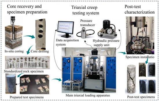
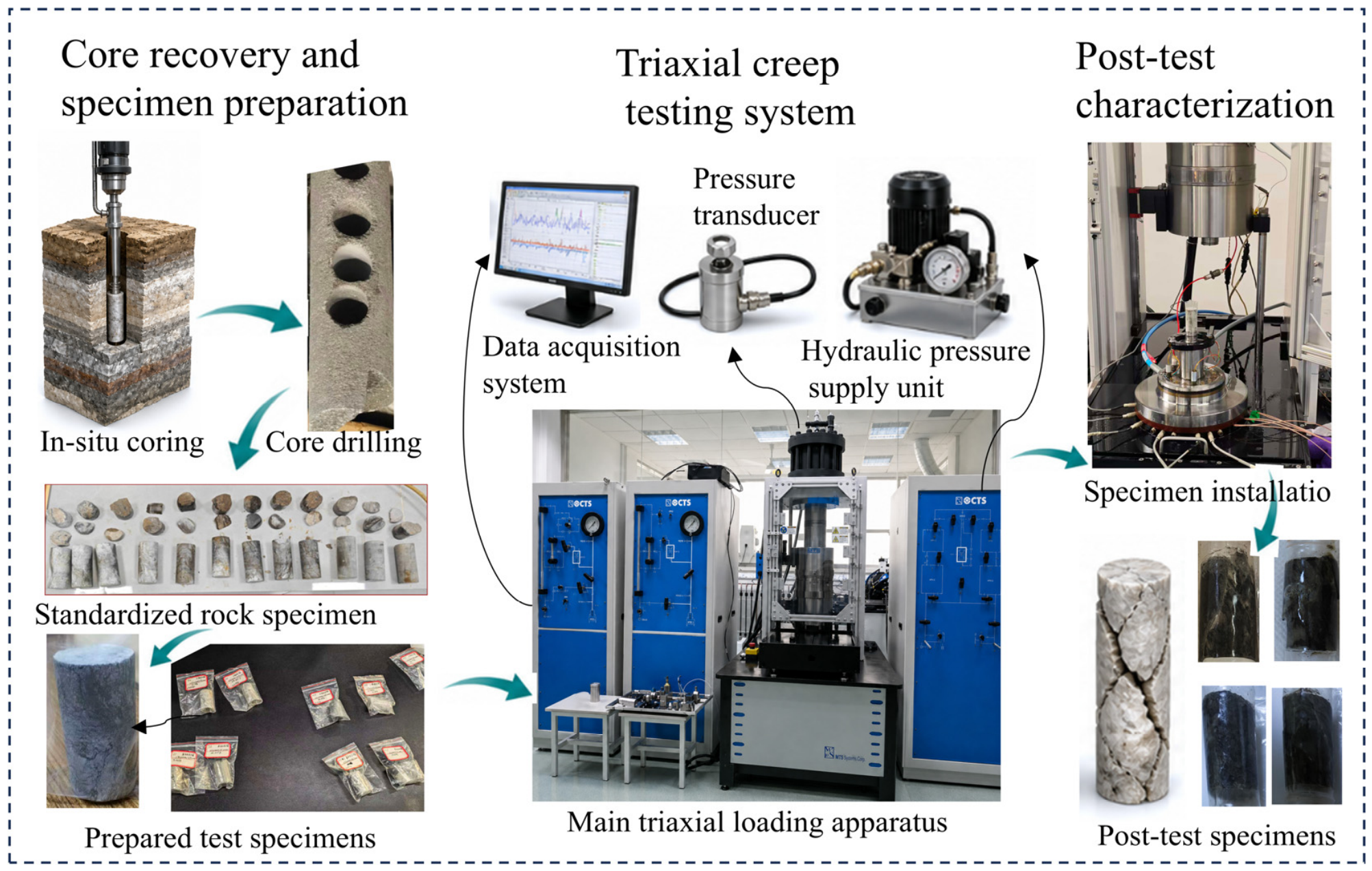
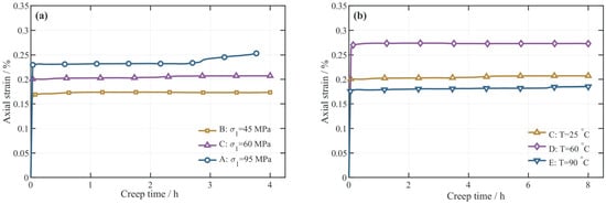
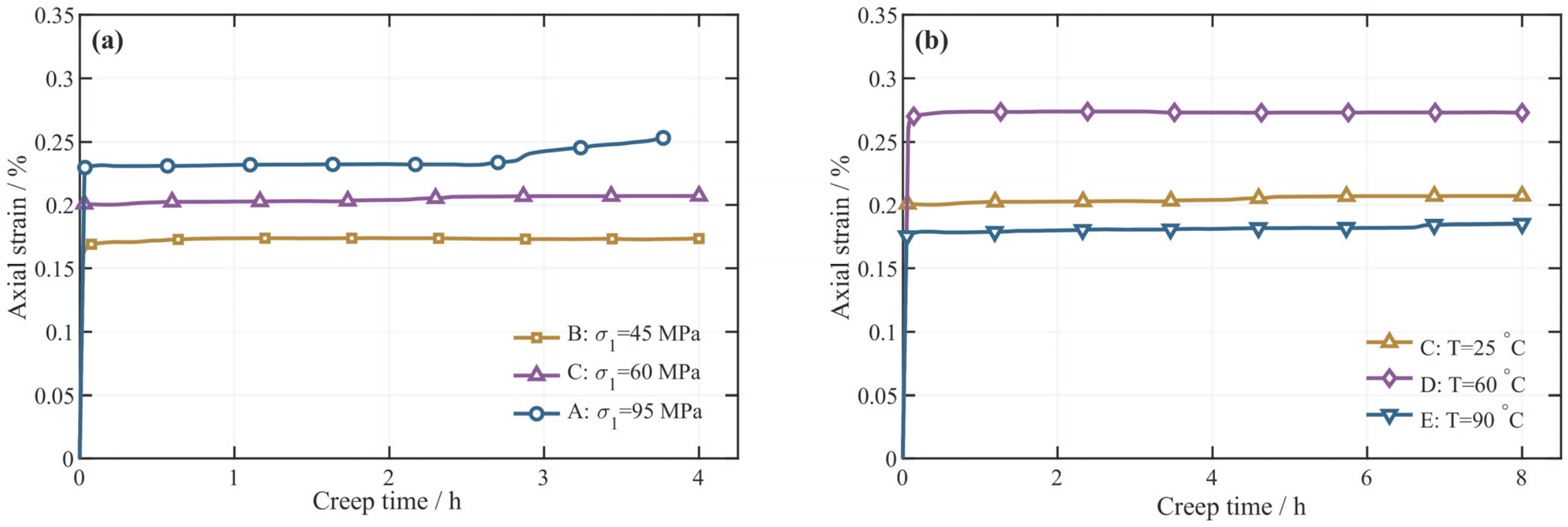
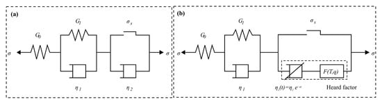
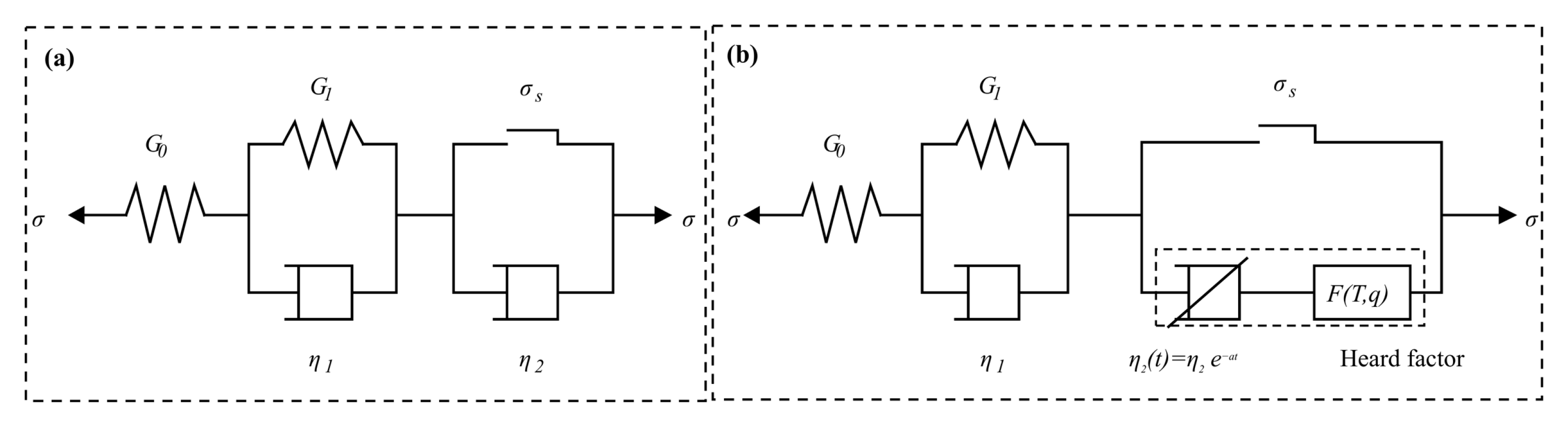
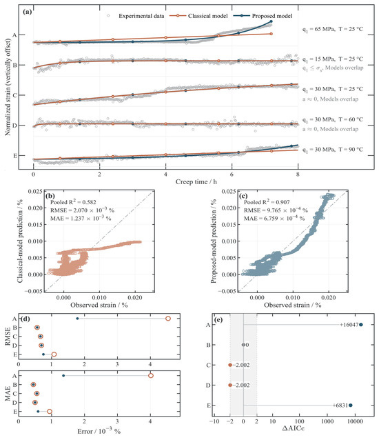
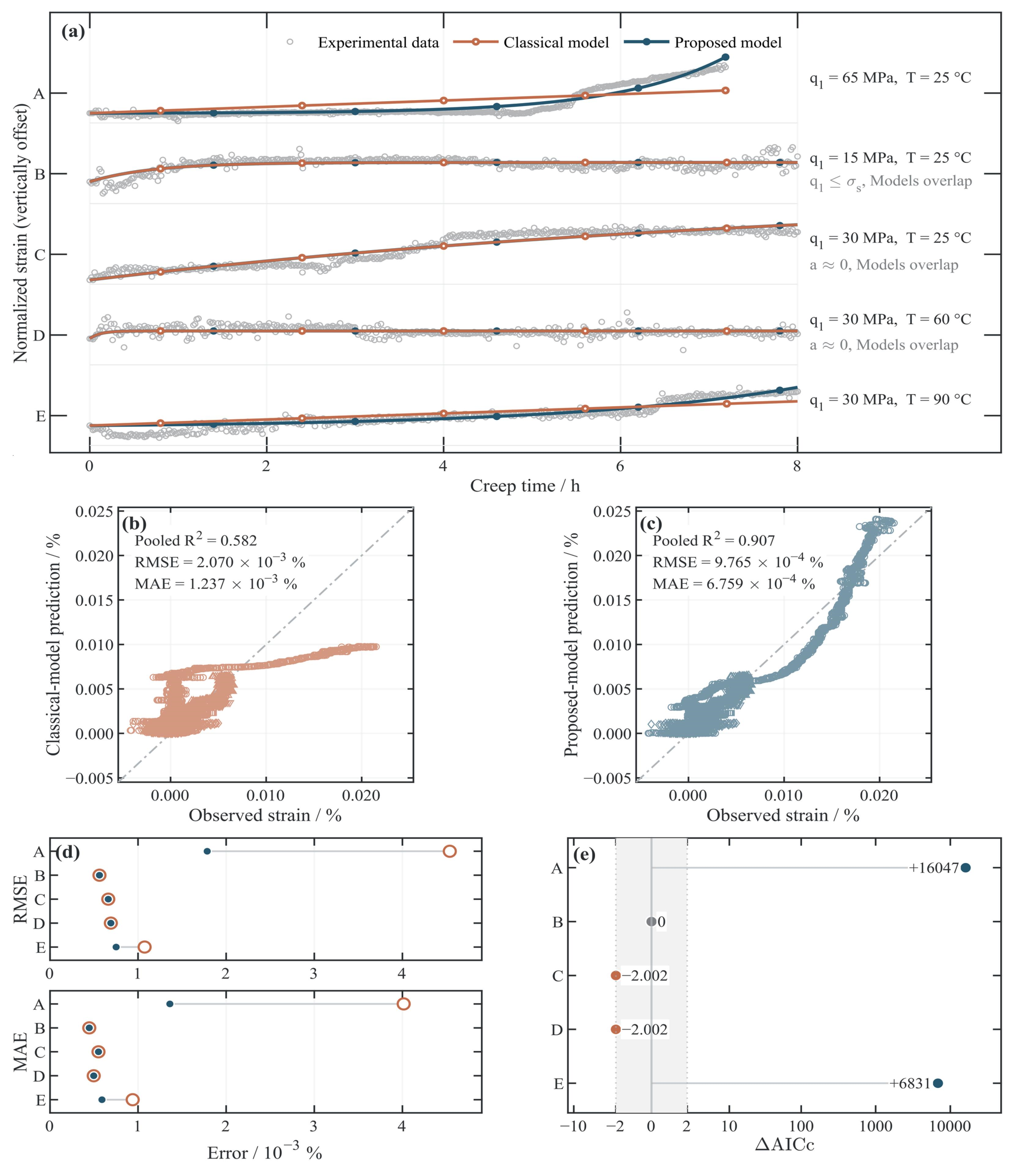
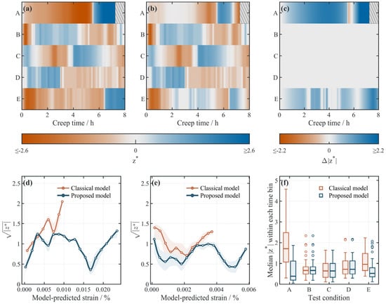
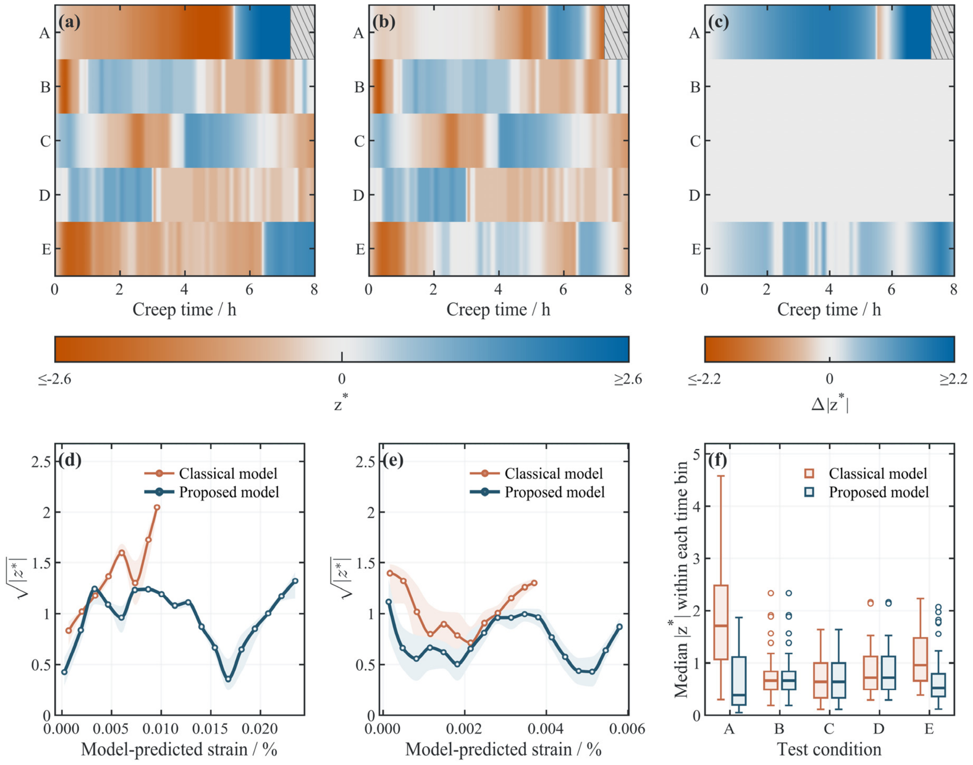
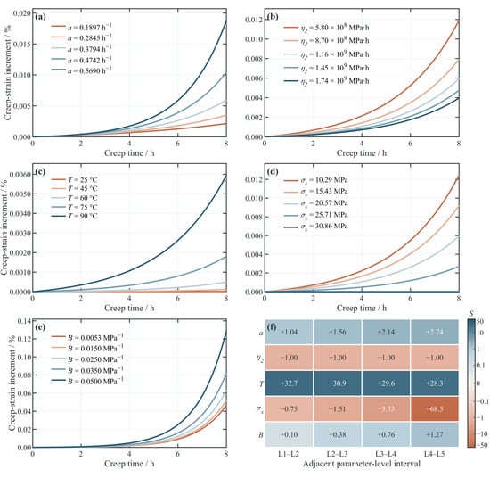
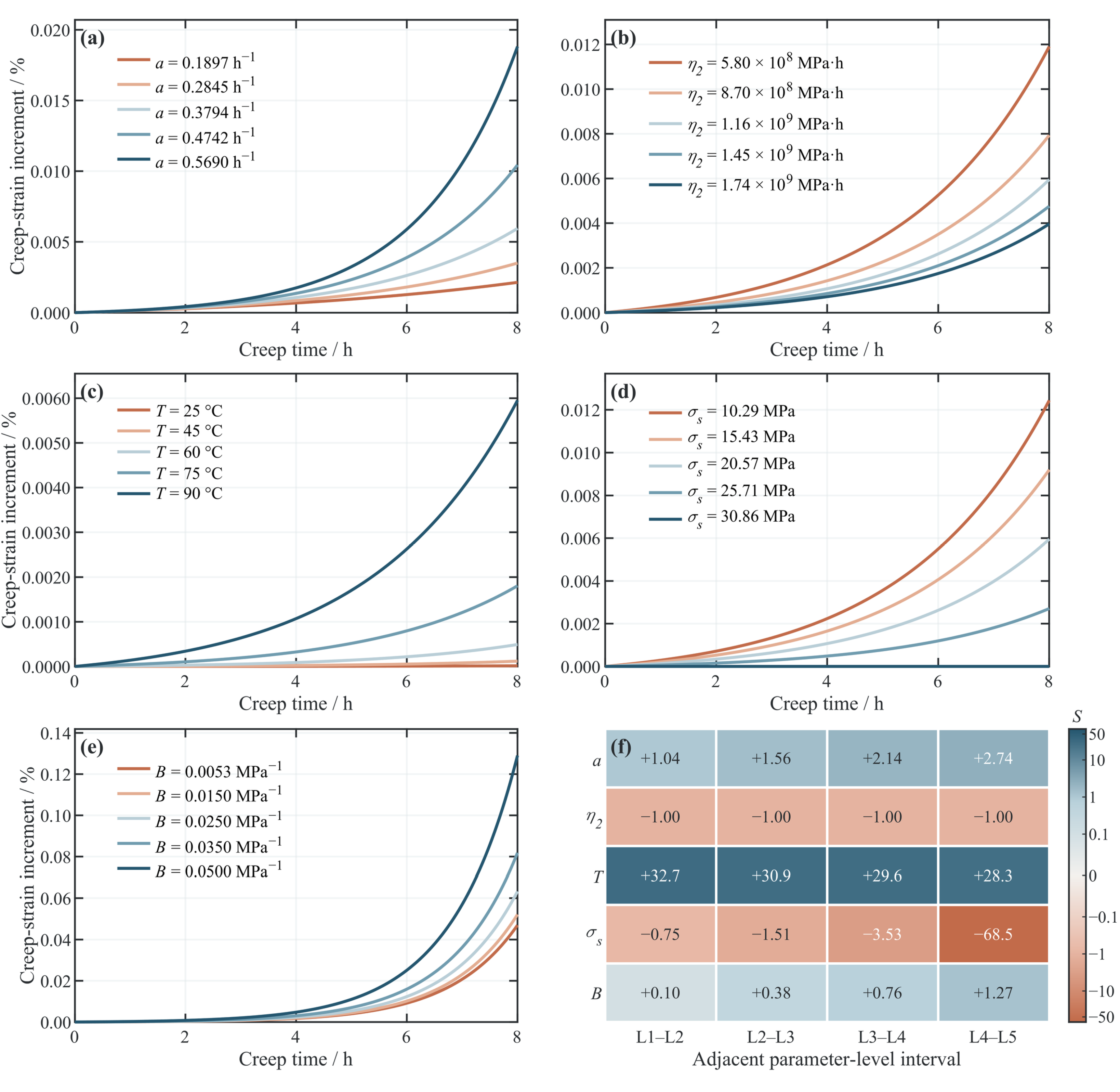
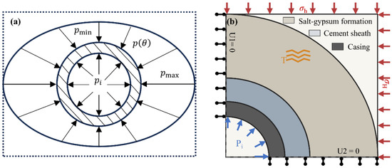
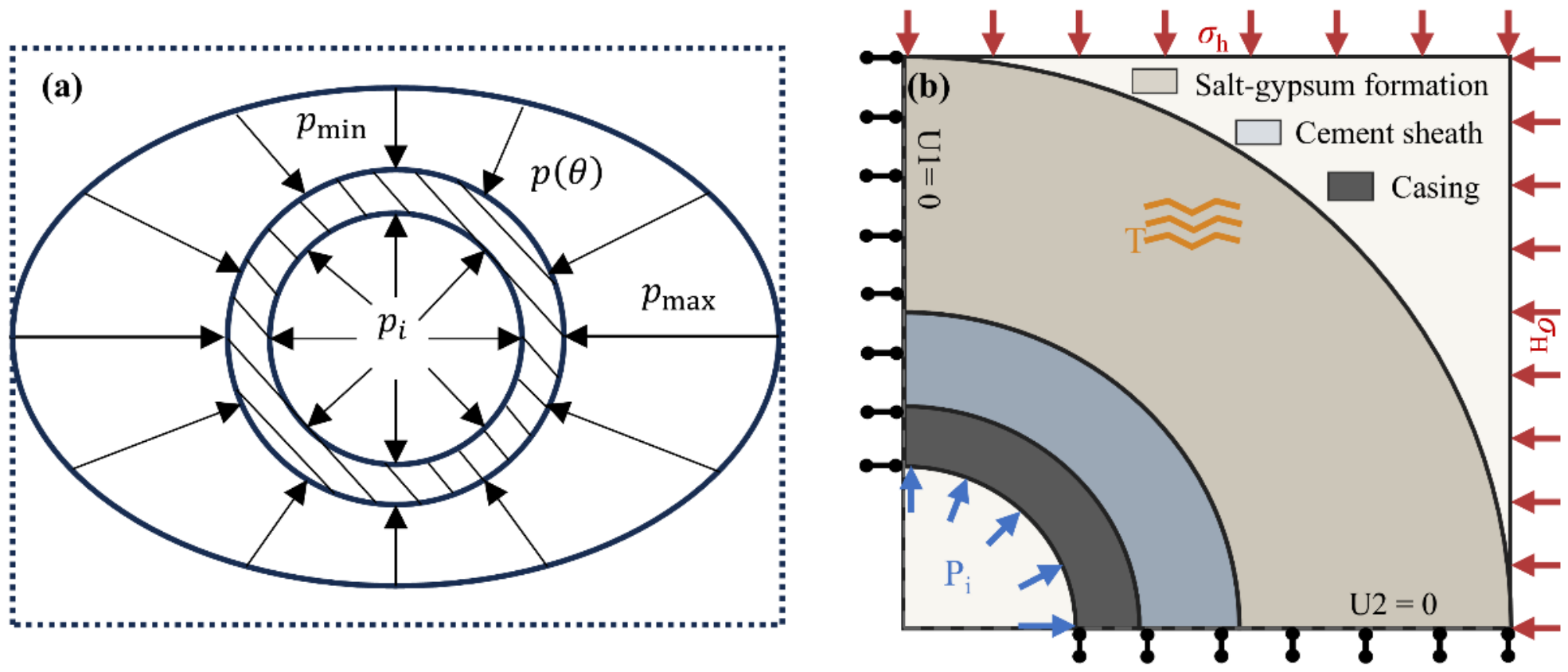
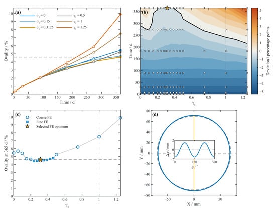
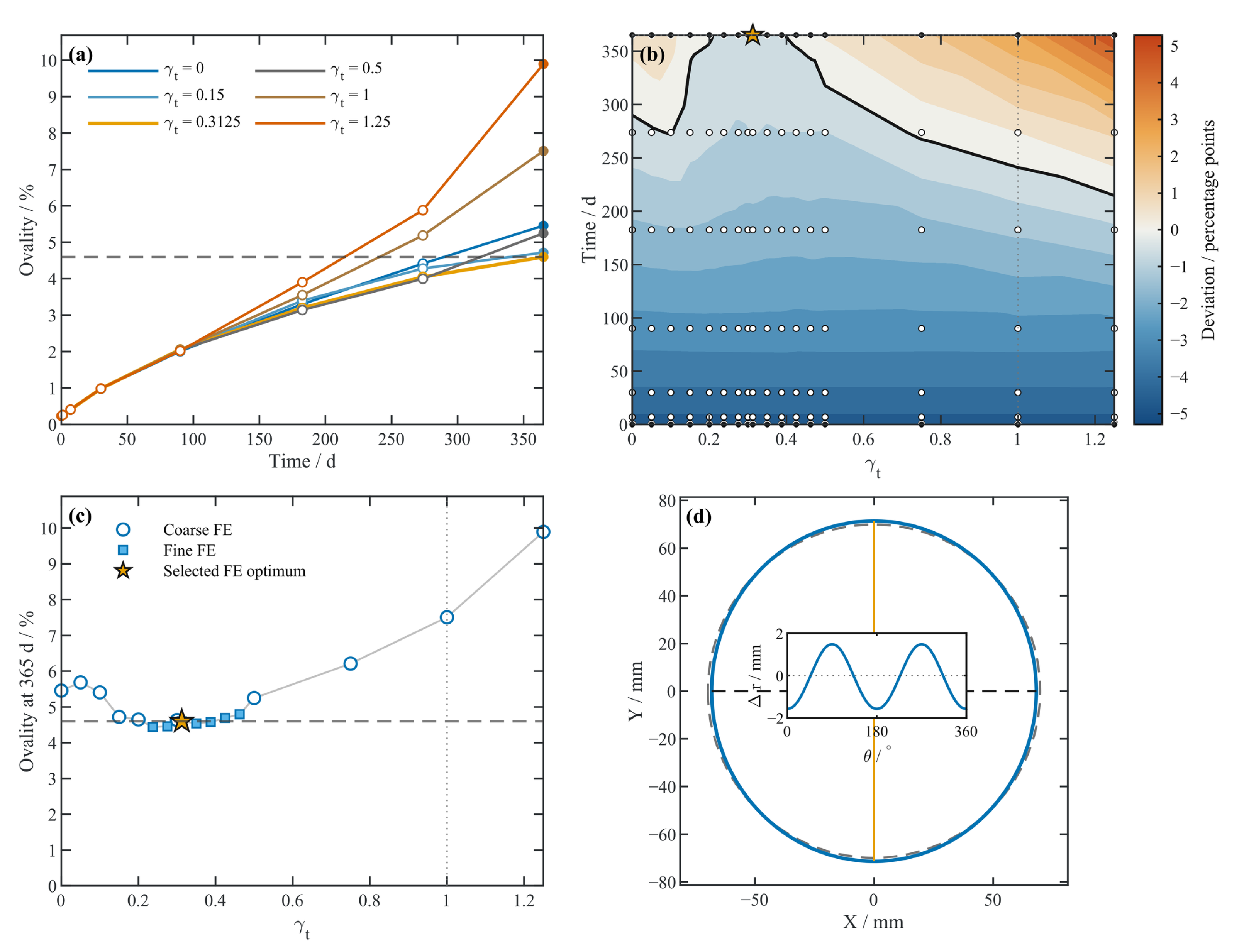
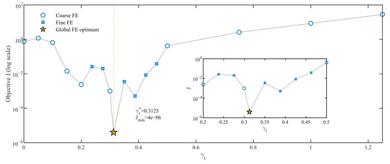
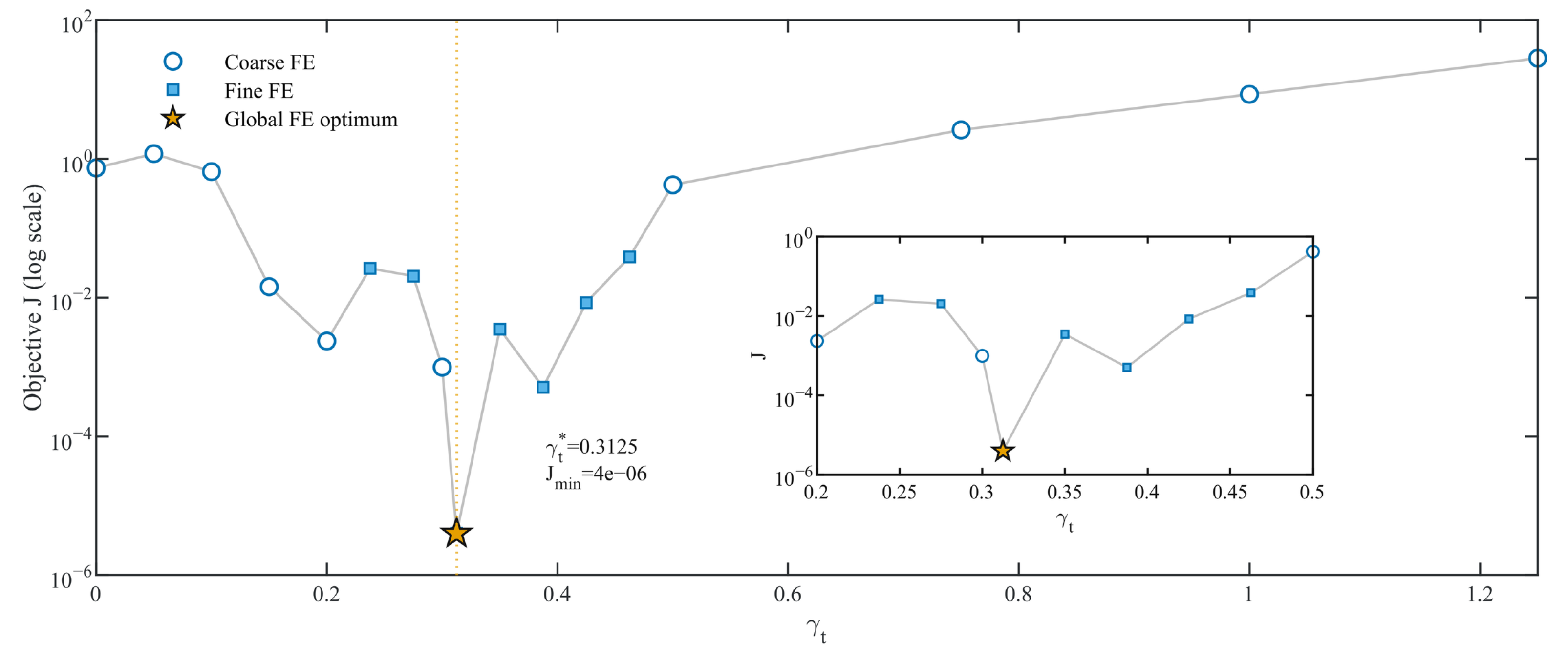
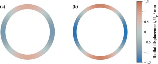
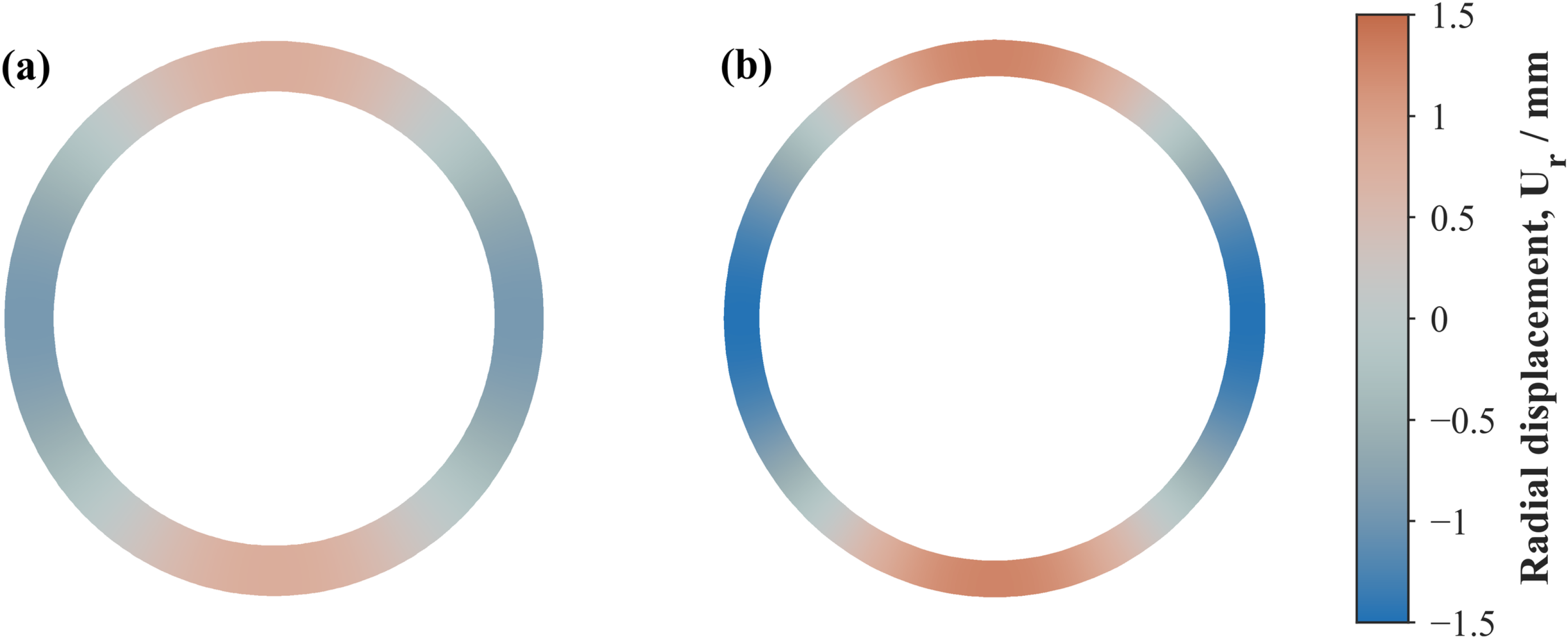

Disclaimer/Publisher’s Note: The statements, opinions and data contained in all publications are solely those of the individual author(s) and contributor(s) and not of MDPI and/or the editor(s). MDPI and/or the editor(s) disclaim responsibility for any injury to people or property resulting from any ideas, methods, instructions or products referred to in the content. |
© 2026 by the authors. Licensee MDPI, Basel, Switzerland. This article is an open access article distributed under the terms and conditions of the Creative Commons Attribution (CC BY) license.