


Abstract
Wind power forecasting under transitional weather conditions is crucial for the secure operation and dispatch of power systems. However, existing methods have limited ability to perceive and adapt to the rapid, nonstationary changes in the weather–power mapping caused by transitional weather, resulting in substantially increased forecasting errors and uncertainty. To address this issue, this paper proposes a day-ahead probabilistic wind power forecasting method based on a weather-transition-aware mixture-of-experts network. First, based on numerical weather prediction (NWP) sequences of wind speed and temperature, a progressive analysis of trends and abrupt changes and a turning-point localization mechanism based on symmetric-ratio minimization are introduced to identify potential transitional periods and generate a weather-transition mask. The binary transition indicator is then concatenated with the NWP features at each time step, and cross-attention is employed to fuse meteorological forecasts with historical power information. Finally, a gated mixture-of-experts (MoE) network dynamically fuses conventional-weather and transitional-weather experts according to the daily transition fraction. Quantile regression is subsequently used to generate prediction intervals at multiple coverage levels. A case study of a wind farm shows that the proposed method achieves a normalized mean absolute error (NMAE) of 5.79%, a coefficient of determination () of 0.88, and a 21.36% reduction in the normalized average width of the 95% prediction interval relative to the baseline with the lowest mean normalized average interval width.
1. Introduction
With the continuous expansion of wind power capacity, the challenges associated with integrating wind power into the grid have become increasingly prominent. Transitional weather characterized by abrupt meteorological changes, such as frontal passages and sudden severe convection, can cause rapid shifts in wind speed and direction, leading to sharp short-term power fluctuations [1,2]. Such sudden increases or decreases in wind power output are known as ramp events [3,4]. These abrupt power changes can reduce the effectiveness of forecasting models trained under conventional conditions, significantly increasing prediction errors. They may also lead to operational risks, such as grid frequency fluctuations and insufficient reserve capacity, threatening power system security [5,6]. Therefore, improving wind power forecasting accuracy under transitional weather conditions is essential for ensuring the secure and stable operation of power systems.
To improve the accuracy and stability of wind power forecasting under transitional weather conditions, existing studies have mainly focused on small-sample modeling, transitional-feature representation, and model adaptability to transitional weather, as discussed below.
Because transitional-weather samples are scarce and typical transitional processes are insufficiently represented, forecasting models may fail to adequately learn rare weather states [7]. Existing research has largely focused on extreme weather. Extreme weather and transitional weather differ in their defining emphasis: the former emphasizes the rarity of an event, whereas the latter emphasizes the evolution of meteorological conditions. Some extreme weather events also involve rapid meteorological changes; therefore, both research areas share challenges in modeling and adaptation under limited-sample conditions. Existing studies have addressed this scarcity through data augmentation and transfer learning. Data-augmentation methods generate large numbers of synthetic power samples using statistical models, including Monte Carlo sampling [8], error-bootstrap oversampling [9], and stratified oversampling [10]. However, because these generated samples depend on the distribution of the original data, they may be affected by sampling bias and other limitations. Consequently, deep generative models, particularly Generative Adversarial Networks (GANs), have been introduced for transitional-scenario modeling [11,12,13], further improving the quality of the generated samples. Reference [14] employs cross-task meta-learning to transfer knowledge acquired by conventional-weather models to extreme-weather forecasting tasks. Reference [15] uses feature transfer by first extracting data features through autoencoder pretraining and then fine-tuning the model with a small number of samples to adapt it to power characteristics under extreme weather. These studies alleviate the problem of insufficient samples, but mainly improve the training-data foundation of the models and still lack a direct description of when future weather will undergo a transition and how intense that transition will be.
Transitional weather is often accompanied by pronounced short-term changes in meteorological variables such as wind speed and wind direction, which can further alter wind power variation patterns. Therefore, accurately identifying transitional periods in future meteorological sequences and enhancing their feature representation are important for improving forecasting performance [16]. Transitional weather describes the evolution of meteorological conditions, whereas wind power ramps represent a possible power response to this process. Ramp event identification studies therefore provide useful insights into characterizing power variations under transitional weather. Related studies on wind power ramp event identification commonly use the Swinging Door Algorithm (SDA) as a foundational framework [17,18]. Reference [19] dynamically adjusts gating parameters and screening mechanisms through a parameter-adaptive strategy to improve the generalization of the identification algorithm, whereas Reference [20] introduces dynamic programming to identify and merge trends in SDA segmentation results, thereby improving identification accuracy. Another line of research focuses on signal segmentation, which adaptively divides continuous power signals according to their fluctuation trends to accurately locate ramp events [21]. Reference [22] combines moving-window trend extraction with pseudo-turning-point identification, whereas Reference [23] develops a two-step segmentation algorithm based on the joint selection of multiple parameters to achieve accurate segmentation and localization of power signals. For key-feature extraction, Reference [24] employs deep architectures, including Convolutional Neural Networks (CNNs), Long Short-Term Memory (LSTM) networks, and Transformers, to extract latent temporal patterns from power sequences and meteorological fields, thereby providing higher-quality input representations for subsequent forecasting models. Reference [25] proposes a Semi-supervised Contrastive Regression Framework (SCRF) that combines pretraining and regression and uses feature-matrix extraction from power sequences to improve forecasting performance. These studies provide a foundation for identifying transition periods and extracting temporal features. However, they differ in their identification targets and the ways in which the extracted information is utilized. Wind power ramp detection primarily characterizes changes in power output and cannot directly substitute for transitional-weather identification. Research on transitional weather, therefore, needs to further clarify how the identified transition information is incorporated into subsequent forecasting models.
Accurate identification and representation of transitional weather provide the basis for improving forecasting performance, whereas continuous optimization of the weather–power mapping is key to further improving forecasting accuracy. Existing model-optimization studies can be broadly classified into physics-informed fusion and segmented optimization strategies [26]. Reference [27] examined diurnal and monthly variations in wind shear coefficients and differences across sites, suggesting that modeling the weather–power relationship should account for temporal variability and site characteristics. Reference [28] embeds NWP model selection and meteorological pattern analysis into the forecasting framework to enhance the use of meteorological forcing information, whereas Reference [29] integrates theoretical power curves with deep architectures to improve forecasting accuracy. Segmented forecasting strategies model different regimes according to the degree of power fluctuations, typically using point forecasting for stable periods and probabilistic forecasting for extreme periods [30,31]. Reference [32] develops a dual-model forecasting system that combines Light Gradient Boosting Machine (LightGBM) and Random Forest (RF) with LSTM, with separate regional models constructed according to regional characteristics. Reference [33] integrates deterministic forecasting with wind power ramp events to develop an LSTM–WPRE–PF framework for day-ahead probabilistic forecasting. It employs wavelet packet variance entropy to analyze uncertainty in power fluctuations, demonstrating progress in combining ramp information with probabilistic forecasting. Overall, existing research has gradually evolved from meteorological feature fusion toward weather-state awareness and uncertainty modeling. However, most existing methods rely on predefined categories for model selection or switching, making it difficult to capture the dynamic evolution of forecasting patterns and uncertainty as weather conditions continuously transition from conventional to transitional weather states. Further research is needed to extract potential transition indicators from future meteorological sequences, incorporate them throughout feature encoding and prediction fusion, and evaluate their effects on forecasting accuracy and prediction interval coverage.
Although the aforementioned studies have made progress in transitional-weather identification accuracy and forecasting performance, several issues remain worthy of further investigation:
- (1)
- Existing methods primarily use transition-identification results for sample partitioning or as ordinary input features. However, how to jointly exploit this information in temporal feature extraction and prediction fusion to enhance the representation of meteorological changes and corresponding power responses during transitional periods remains to be investigated.
- (2)
- Wind power ramp detection and transitional-weather identification focus on different targets, and labels derived from the former cannot directly substitute for those of the latter. How to jointly characterize trends, abrupt changes, and fluctuations using NWP sequences available for day-ahead forecasting, thereby accurately identifying transitional periods, is a key challenge in developing transition-aware forecasting models.
- (3)
- Existing segmented forecasting methods can select or switch between different models according to predefined weather categories. However, they struggle to capture the gradual evolution of forecasting patterns as weather conditions continuously shift from conventional to transitional weather states. Furthermore, they have difficulty dynamically adjusting the contributions of different forecasting models according to the daily transition fraction, resulting in insufficient adaptability of forecasting results and prediction intervals during transitional weather conditions.
To address these issues, this paper proposes a transition-aware method for day-ahead probabilistic wind power forecasting. Weather-transition information extracted from the NWP forecast sequence is used as an explicit input feature to guide the model in adaptively adjusting the weather–power mapping and forecasting strategy, thereby enabling accurate prediction of wind power and its uncertainty under complex weather conditions.
The main contributions of this paper are threefold:
- (1)
- A transitional-weather identification method based on the synergistic coupling of multidimensional meteorological features is proposed. Through progressive analysis of trend and abrupt-change features and symmetric-ratio-minimization-based turning-point localization, potential transitional-weather periods in future meteorological sequences are identified, providing explicit transition indicators for weather-state representation and subsequent power forecasting.
- (2)
- A transition-indicator-driven feature-enhancement mechanism for transitional-weather processes is developed. The binary transition indicator is concatenated with the NWP features at each time step, providing explicit information about potential transitional periods, and cross-attention is used to strengthen the coupled representation of meteorological evolution and historical power responses during transitional periods, thereby improving forecasting accuracy under transitional weather.
- (3)
- A probabilistic wind power forecasting method based on a mixture of forecasting experts for different weather types is proposed. Dedicated experts are constructed for conventional and transitional weather, expert weights are adaptively assigned according to the daily transition fraction, and joint multi-quantile forecasting is used to dynamically characterize power uncertainty, enabling adaptive construction of prediction intervals under different weather states.
2. Method
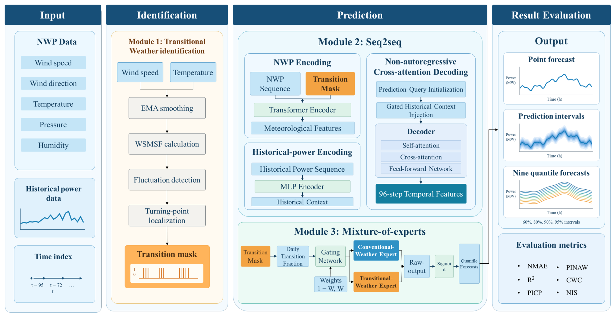
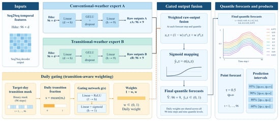
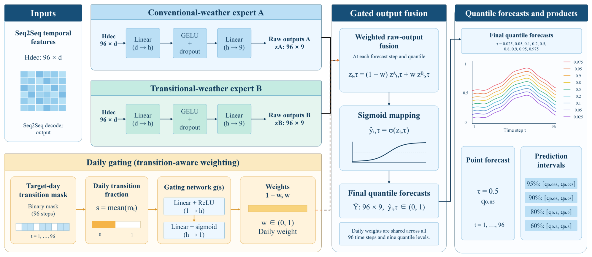
This paper constructs the forecasting framework at three progressive levels: weather-state identification, temporal dependency modeling, and adaptive uncertainty quantification. The overall framework is shown in Figure 1.
Figure 1.
Overall framework.
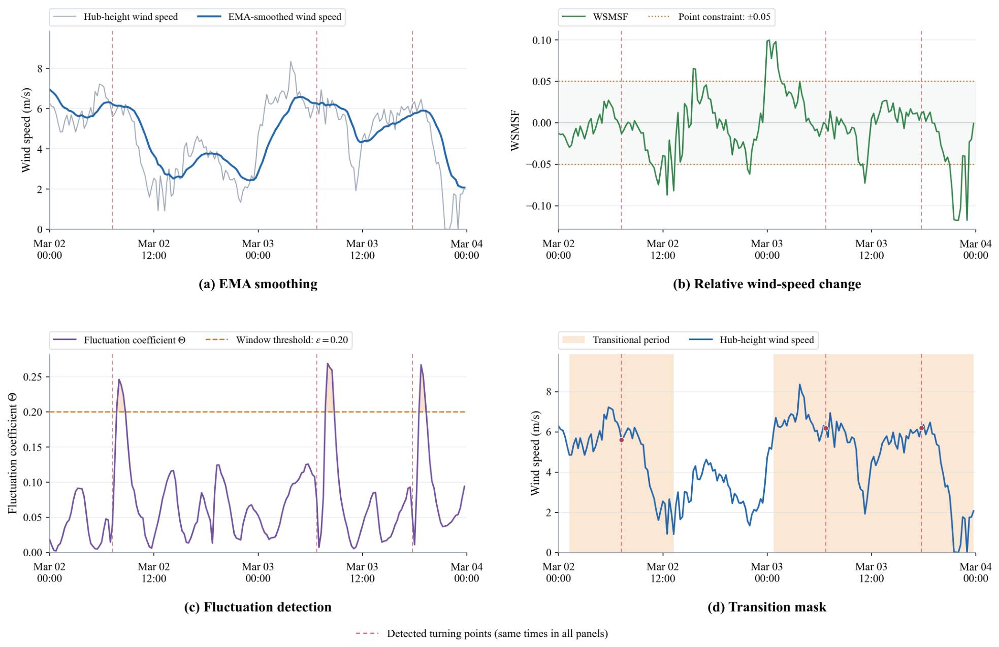
The first module takes the NWP wind-speed and temperature sequences for the target forecasting day as inputs and generates a transition mask through four sequential steps: EMA smoothing for trend extraction, WSMSF calculation for relative wind-speed change quantification, fluctuation-coefficient calculation for detecting potential transitional-weather intervals, and turning-point localization for generating the final mask. The binary transition indicator is then concatenated with the NWP features at each time step as an additional encoder input feature. The second module constructs an NWP-driven non-autoregressive Sequence-to-Sequence (Seq2Seq) architecture: a Transformer encoder extracts the global context of multidimensional meteorological sequences, a Multilayer Perceptron (MLP) encoder compresses historical power into a context vector, and a cross-attention decoder generates temporal representations for the next 96 steps in parallel. The third module introduces a transition-aware mixture-of-experts network, which dynamically fuses the outputs of conventional-weather and transitional-weather expert branches according to the daily transition fraction and outputs prediction intervals at multiple nominal coverage levels through quantile regression.
2.1. Transitional-Weather Identification
Transitional weather in this study refers to processes in which the trends or statistical characteristics of meteorological conditions change significantly over a timescale of several hours, with an emphasis on meteorological evolution. Because transitional weather involves changes in multiple meteorological factors [34], a transitional-weather identification module based on the joint assessment of multidimensional meteorological features is developed. To balance the complexity and reliability of the identification module, wind speed and temperature are selected as transition detection variables to jointly characterize wind field variations and their thermal background. Wind speed is directly related to power variations, while temperature provides supplementary information on meteorological evolution. The identified transitions represent potential transitional weather from a forecasting perspective, reflecting weather-state changes that may occur based on the meteorological forecast information available at the prediction time.
2.1.1. Trend Extraction and Fluctuation Quantification
To suppress high-frequency disturbances in the NWP sequence while preserving its overall trend, an exponential moving average (EMA) with a span of N is applied to the wind-speed and temperature sequences:
where t denotes the current time step and is the smoothing coefficient. On this basis, the wind-speed mutation sensitivity factor (WSMSF) is defined to quantify the instantaneous relative rate of change in the wind-speed sequence:
where denotes the EMA-smoothed wind speed at time t, and is a small constant introduced to avoid division by zero. The sign of the WSMSF indicates whether wind speed is increasing or decreasing, whereas its absolute value reflects the severity of the change in wind speed.
2.1.2. Multidimensional Sliding-Window Fluctuation Coefficient
The EMA or WSMSF of a single variable cannot fully describe the multidimensional coupling characteristics of a weather system. Transitional weather is often accompanied by coordinated changes in multiple variables. Therefore, a multidimensional sliding-window fluctuation coefficient is constructed. The smoothed wind-speed and temperature sequences are arranged into a data matrix using windows of length L. For the kth window, the mean vector and standard-deviation vector are calculated for each feature, and the range of each feature over the full sequence, denoted by , is used for normalization. The inter-window differences in the means and standard deviations are defined as follows:
The sliding-window fluctuation coefficient is defined as the larger of the normalized inter-window differences in the mean and standard deviation:
When the coefficient exceeds the preset threshold , the window is marked as a potential transitional-weather interval containing a potential abrupt turning point and is included in the candidate set for subsequent turning-point localization.
2.1.3. Turning-Point Localization and Transition Mask Generation
Within each candidate interval, potential turning-point positions are evaluated using two adjacent subwindows immediately before and after each position. Each subwindow has a length of . The symmetric ratio (SR) between the two subwindows is defined as follows:
where and denote the EMA-smoothed wind-speed values at the jth position in the left and right subwindows, respectively.
A smaller SR indicates a smaller normalized difference between the wind-speed values at corresponding positions in the two subwindows. Candidate positions are restricted to those satisfying , and the position with the minimum SR is selected as the turning point within each candidate interval.
After all turning points have been identified, a potential transitional-weather period is generated around each turning point by extending H time steps in each direction. The covered time steps are labeled as transitional states to form the transition mask, which provides explicit transition indicators for subsequent forecasting. The parameter settings of the identification module are listed in Table 1.
Table 1.
Parameter settings of the transitional-weather identification module.
These parameters are mainly determined by the data sampling frequency, the timescale of weather transitions, and the requirements for smoothing, fluctuation detection, and event coverage. The EMA span is set to 16 (smoothing coefficient: 0.118) to suppress short-term noise while preserving overall trends. The 24-step sliding window (6 h) captures representative local variations and supports statistical feature extraction. The fluctuation threshold is set to 0.20 to balance detection sensitivity and false positives, and its impact on forecasting performance is assessed through sensitivity analysis. Each detected turning point is extended by 24 steps (6 h) in both directions to capture the full transition process and avoid missing relevant changes.
2.2. Transition-Aware Seq2Seq-MoE Forecasting Model
A Seq2Seq-MoE forecasting model is proposed. The multidimensional NWP sequence serves as the primary driving signal, historical power serves as an auxiliary condition, and the transition mask provides an explicit transition indicator as an additional encoder input feature. The Seq2Seq architecture generates temporal representations for the future prediction horizon, while the mixture-of-experts network uses separate expert branches for conventional and transitional weather. A gating network dynamically fuses the outputs of the two branches according to the daily transition fraction, enabling adaptive characterization of prediction intervals under different weather patterns.
2.2.1. Seq2Seq Architecture
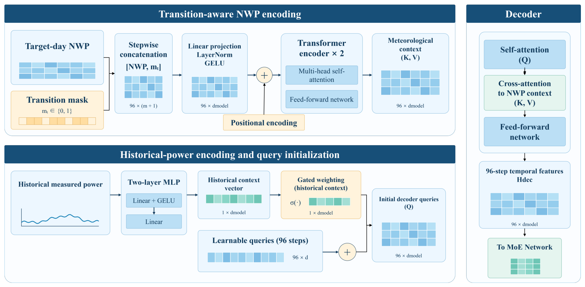
An NWP-driven, non-autoregressive Seq2Seq architecture is adopted to forecast wind power over the next 96 time steps. The model consists of an NWP encoder, a historical-power encoder, and a cross-attention decoder. The NWP encoder extracts temporal features from the meteorological data, the historical-power encoder provides auxiliary information about the previous day’s power variations, and the decoder generates forecasts from these two sources of information. The overall Seq2Seq architecture is shown in Figure 2.
Figure 2.
Schematic of the Seq2Seq architecture.
The NWP encoder is built around a Transformer and extracts global temporal context from the meteorological sequence for the target forecasting day. At each time step, multidimensional NWP features are concatenated with the corresponding transition mask value to form a transition-aware input vector. This preserves the temporal alignment between meteorological features and transition indicators while retaining information from all time steps, allowing the model to learn their relationships. The concatenated features undergo linear projection, layer normalization, and nonlinear transformation, followed by positional encoding and Transformer encoding. The mask thus explicitly indicates potential transitional periods during temporal feature extraction. The historical power encoder uses a two-layer MLP to compress the historical measured power sequence available at the forecast issuance time into a context vector, which is added to the learnable query vector at each forecast step after gated weighting to form the initial decoder queries.
The decoder adopts a non-autoregressive structure. Through cross-attention, it extracts meteorological information relevant to each forecasting time step from the NWP encoder outputs while incorporating the historical-power context to generate temporal features for the next 96 steps. The decoder output is then fed into the mixture-of-experts network, which fuses forecasts under different weather states.
2.2.2. Mixture-of-Experts Network
To enable the model to adjust its forecasting strategy according to the weather state, a weather-state-driven mixture-of-experts network is introduced after the Seq2Seq decoder. Two separately parameterized forecasting branches are established: a conventional-weather expert () and a transitional-weather expert (). The two experts are dynamically fused according to the daily transition fraction. The structure is shown in Figure 3.
Figure 3.
Schematic of the mixture-of-experts network.
Let the stepwise transition mask sequence for the target day be denoted by , where 1 indicates a transitional period. The daily transition fraction s is defined as the mean of the mask sequence, representing the proportion of forecast time steps identified as transitional:
The input s is fed into a two-layer fully connected gating network. After ReLU activation and sigmoid mapping, the gating weight w is obtained as follows:
Given the temporal features produced by the decoder, the conventional-weather and transitional-weather experts independently generate raw outputs and for each forecast time step t and quantile level . These outputs are combined using the daily gating weight w, and the fused raw output is then mapped to the normalized power range by a sigmoid function:
Here, denotes the fused raw output, denotes the sigmoid function, and denotes the final normalized quantile forecast. The same daily gating weight is shared across all forecast time steps and quantile levels. The forecasting network is jointly trained by applying quantile loss to the final forecasts , and prediction intervals are constructed from the corresponding lower and upper quantile forecasts.
This network propagates the transitional-weather identification results from the input features to the forecasting output, thereby establishing a direct link between the weather state and the expert forecasting strategy. The conventional-weather expert is designed to capture power variations under stable weather, whereas the transitional-weather expert is designed to capture the stronger power fluctuations and greater forecasting uncertainty associated with transitional weather. By dynamically fusing the two experts, the model maintains point-forecasting accuracy while adaptively adjusting the predicted quantiles and prediction-interval width according to the daily transition fraction, thereby improving uncertainty characterization under transitional weather.
2.3. Training Strategy and Loss Function
The Seq2Seq-MoE forecasting network is trained end-to-end using the precomputed transition mask as a fixed input feature. The transition mask is generated by the transitional-weather identification algorithm and is directly concatenated with the NWP encoder input as a fixed feature during training. The Seq2Seq-MoE forecasting model is jointly optimized, with the quantile loss serving as the primary objective for multi-quantile prediction:
where denotes the asymmetric quantile-regression loss at the qth quantile level , and Q is the number of quantiles. A gating-entropy regularization term is also introduced to prevent the gating weight from collapsing to 0 or 1:
where is a small constant to avoid taking the logarithm of zero.
The final training loss is obtained by linearly combining the primary loss and the gating-entropy regularization term:
An entropy regularization coefficient is introduced to prevent the gating weights from prematurely approaching 0 or 1 and reduce the risk of one expert branch consistently receiving low weights. This regularization encourages both branches to participate in training. An excessively large coefficient may drive the weights toward 0.5, weakening the gate’s response to the daily transition fraction, whereas an excessively small coefficient may increase the risk of gate saturation and imbalanced branch training. During training, the gating weight w dynamically adjusts the learning contributions of the two experts according to the daily transition fraction, allowing the two expert branches to develop differentiated forecasting capabilities through iterative optimization. The model is optimized using Adam with decoupled weight decay (AdamW), with an initial learning rate of and a cosine-annealing schedule with warm restarts. The core hyperparameter settings are listed in Table 2.
Table 2.
Hyperparameter settings.
The model outputs nine quantiles, , with the quantile used as the point forecast. The quantile pairs , , , and form the 95%, 90%, 80%, and 60% prediction intervals, respectively.
3. Case Study
3.1. Evaluation Metrics
To comprehensively evaluate the proposed method in terms of point-forecasting accuracy and probabilistic prediction-interval quality, an evaluation framework is established from three perspectives: forecast error, interval coverage, and interval width.
3.1.1. Point-Forecasting Metrics
The normalized mean absolute error (NMAE) is defined as follows:
where T denotes the number of forecast time steps per sample; denotes the installed capacity of the wind farm; denotes the measured power; denotes the corresponding median forecast.
The coefficient of determination () is defined as follows:
where denotes the mean of all measured power values; is the number of forecast samples, and and are the measured power and median forecast for sample i at time step t, respectively.
3.1.2. Probabilistic-Forecasting Metrics
The prediction interval coverage probability (PICP) measures the proportion of actual power values that fall within the prediction interval:
where is an indicator variable that takes a value of 1 if the actual value falls between the lower and upper bounds of the prediction interval and 0 otherwise.
The prediction interval normalized average width (PINAW) measures the average width of the prediction interval and reflects the sharpness of the interval forecast:
where and denote the upper and lower bounds of the prediction interval, respectively.
The coverage width-based criterion (CWC) jointly evaluates the balance between interval coverage and interval width:
where denotes the nominal coverage level, and denotes the penalty coefficient.
The Normalized Interval Score (NIS) jointly evaluates prediction interval width and the deviation of observations falling outside the intervals.
where is the nominal coverage level. and are indicator functions that determine whether the actual power falls below or above the prediction interval, respectively. Specifically, when , and 0 otherwise; when , and 0 otherwise. Both indicators are 0 when the actual power lies within the prediction interval. NIS penalizes observations outside the prediction interval while evaluating interval width, thereby capturing the severity of undercoverage and complementing CWC.
3.2. Dataset
Historical measured data from a 99 MW wind farm and NWP data provided by the European Centre for Medium-Range Weather Forecasts (ECMWF) are used. The data have a temporal resolution of 15 min and a spatial resolution of 9 km. All NWP forecasts used for prediction are available before forecast issuance. Each forecast uses a fixed NWP forecast vintage for the target horizon, without incorporating meteorological observations, measured power, or subsequent NWP updates obtained after issuance.
First, the data are sorted chronologically, duplicate timestamps are removed while retaining the first record, and a complete time series is reconstructed at 15-min intervals. Power and meteorological variables are clipped to physically reasonable ranges, and missing values are handled by temporal interpolation. Records with remaining missing values are removed, and temporal continuity is checked during sample construction. The dataset is then divided by using the data from four months in 2020—March (spring), June (summer), September (autumn), and December (winter)—as the test set, while data from all remaining months are used for training. The power data are normalized by the installed capacity, whereas the NWP features are normalized using min–max normalization. The minimum and maximum values are determined exclusively from the training data, and the same normalization parameters are applied to the test set. Finally, the processed data are divided into samples using a sliding-window approach, with one day serving as the basic sampling unit.
3.3. Transitional-Weather Identification Result
Following Section 2.1, windows with fluctuation coefficients above 0.2 are identified as candidate transitional-weather intervals. Within each interval, the position with the minimum symmetric ratio is selected as the turning point. Extending 24 time steps in each direction from each turning point defines potential transitional periods and generates the transition mask. The training and test sets contain 205 and 42 turning points, respectively, with transitional periods covering 13.4% and 12.9% of their time steps.
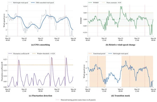
Figure 4 illustrates the four-stage transitional-weather identification process using 2–3 March 2020, as an example: EMA smoothing for trend extraction, WSMSF for quantifying relative wind-speed changes, the fluctuation coefficient for detecting potential transitional-weather intervals, and turning-point localization for generating the final mask.
Figure 4.
Four-stage transitional-weather identification process.
3.4. Overall Forecasting Performance Comparison
To evaluate the contributions of transitional-weather identification, the transition mask, and the mixture-of-experts mechanism to forecasting accuracy and uncertainty characterization, the proposed method is compared with eight baseline models: MLP, CNN, LSTM, CNN-LSTM, Transformer, Informer, XGBoost, and bidirectional long short-term memory (BiLSTM). These baselines cover five major architectural categories: fully connected, convolutional, recurrent, self-attention, and tree-based models. All models use the same inputs as the proposed method, output probabilistic forecasts for 96 time steps and nine quantiles, and are trained using quantile loss.
3.4.1. Point-Forecasting Results
The point-forecasting metrics of all models are summarized in Table 3.
Table 3.
Point-forecasting results of the models.
Table 3 presents the point-forecasting results of each model across three different random seeds, reported as mean ± standard deviation. The experimental results show that the proposed method achieves the best performance on both point-forecasting metrics, with an NMAE of 5.79% and an of 0.88. The proposed method achieves a lower NMAE than the best-performing Transformer model, reducing the NMAE from 6.07% to 5.79%, corresponding to a reduction of 4.61%. This result demonstrates the effectiveness of the proposed method in reducing forecasting errors. The proposed method also achieves a higher than the CNN-LSTM, Transformer, and Informer models, indicating that it not only reduces the average forecasting deviation but also more adequately explains the overall variation in wind power. MLP and XGBoost exhibit larger average forecasting errors and lower values. Although the deep-learning models LSTM, BiLSTM, and CNN improve both metrics, their overall performance remains inferior to that of the proposed method. Overall, the proposed method more effectively captures temporal variations in wind power, reduces forecasting deviations, and achieves superior point-forecasting accuracy compared with all benchmark models.
3.4.2. Probabilistic-Forecasting Results
The 95% prediction-interval results of all models are presented in Table 4. Results are reported as the mean and sample standard deviation across three random seeds. Each metric, including CWC, is calculated separately for each seed before aggregation.
Table 4.
Prediction-interval results of the models for the 95% prediction interval.
The proposed method achieves a mean PICP of 95.38%, close to the nominal 95% level, with the lowest PINAW, CWC, and NIS values of 0.30, 0.30, and 0.38, respectively. XGBoost exhibits undercoverage, with a PICP of 89.95%, whereas the other baseline models exceed the nominal coverage level but produce wider intervals. The proposed method reduces PINAW by 21.36–37.23%, CWC by 21.36–95.38%, and NIS by 14.09–47.08% relative to the baselines, indicating a better balance between coverage and interval sharpness.
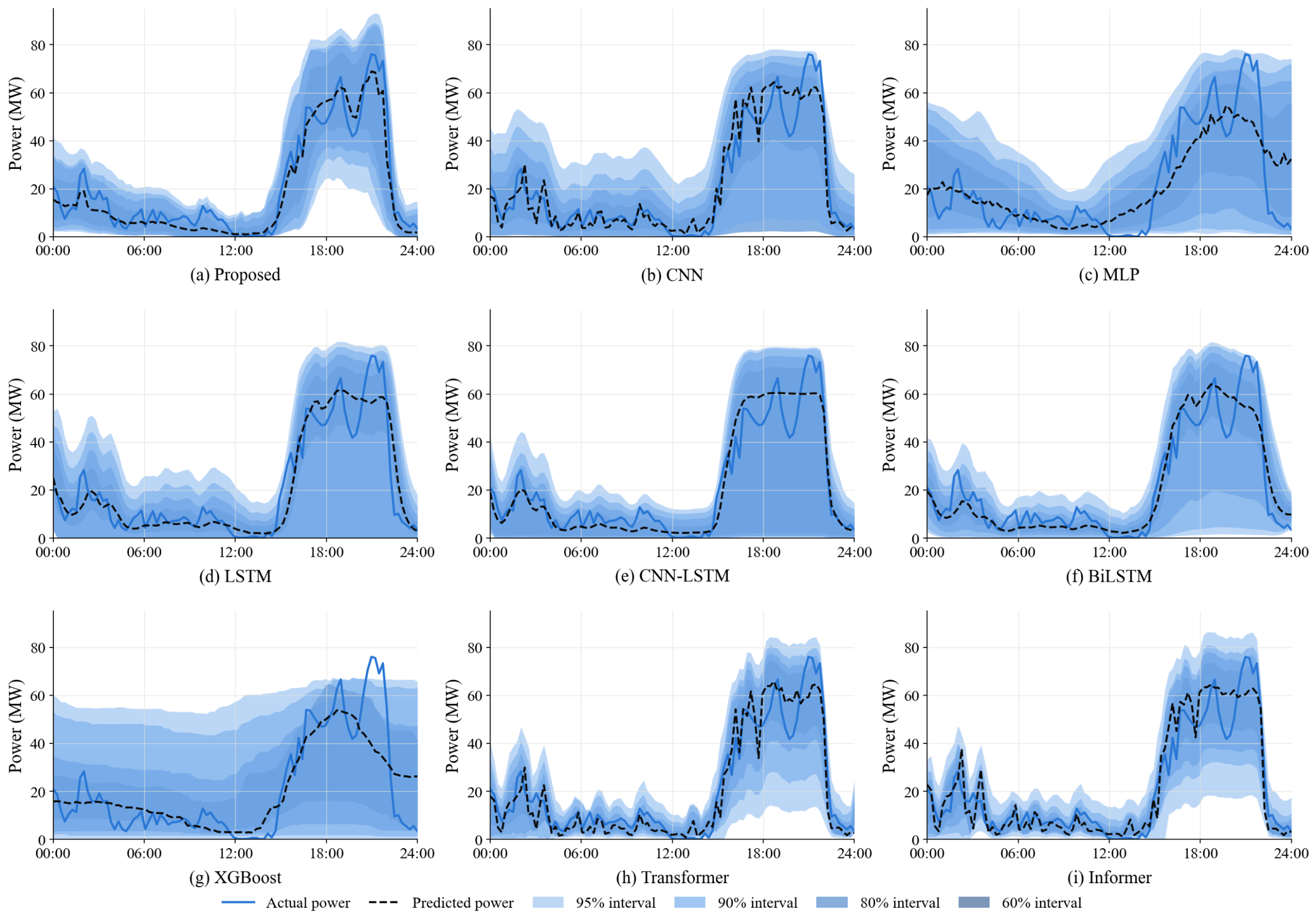
The forecasting data for 21 June 2020 are selected for visualization, as shown in Figure 5.
Figure 5.
One-day probabilistic forecasting results of the models.
Figure 5 presents the one-day probabilistic wind power forecasting results of all models. The blue solid line represents the actual power, the black dashed line represents the point forecast, and blue shaded regions of different intensities represent multi-level prediction intervals ranging from 60% to 95%. Compared with the CNN, MLP, XGBoost, Transformer, Informer, LSTM, BiLSTM, and CNN-LSTM benchmark models, the proposed method tracks wind power variations more accurately and better captures transition processes such as sharp power increases, peak oscillations, and rapid declines. MLP and XGBoost capture only the general power trend and exhibit delayed responses to abrupt power changes. LSTM-based models show noticeable forecasting deviations at peak values. CNN, Transformer, and Informer capture most power-fluctuation trends but exhibit excessively high oscillations. Moreover, the prediction intervals of the benchmark models are excessively wide, resulting in conservative uncertainty estimates. The proposed method adaptively adjusts the interval width according to the degree of power fluctuation, maintaining narrower intervals during stable periods and moderately widening them during intense fluctuations. For this example, the proposed method provides prediction intervals that adapt to the observed power variations while closely tracking the power trajectory.
3.5. Forecasting Performance Under Different Weather Types
The forecasting performance under different weather types is further analyzed by dividing the test samples into transitional-weather days and conventional-weather days for separate statistical evaluation. A day is classified as a transitional-weather day if more than 20% of its time steps are identified as potential transitional weather, reflecting the degree of potential meteorological changes from a forecasting perspective. In the test set, 30 transitional-weather days and 91 conventional-weather days are identified. The interval-forecasting evaluation uses the same weather labels and the same three runs as in Table 4. Each interval metric is calculated separately for each seed within each weather subset and then averaged across the three seeds.
Conventional-weather days have an NMAE of 5.42% and an of 0.89, compared with 6.90% and 0.84 on transitional-weather days. The larger errors on transitional-weather days indicate that their power variations remain more difficult to predict. To evaluate the model’s ability to adaptively characterize forecasting uncertainty under transitional weather, interval-forecasting metrics are calculated for the 95%, 90%, 80%, and 60% prediction intervals, as summarized in Table 5.
Table 5.
Mean prediction-interval performance under different weather types.
On transitional-weather days, the mean coverage rates of the 95% and 90% prediction intervals are 94.33% and 89.11%, respectively, falling below their nominal levels by 0.67 and 0.89 percentage points. The 80% and 60% intervals have mean coverage rates of 83.00% and 60.20%. Compared with conventional-weather days, transitional-weather days have wider intervals at all four levels, with PINAW ranging from 0.14 to 0.33 and NIS from 0.26 to 0.45. Despite meeting their nominal coverage levels on average, the 60% interval on transitional-weather days and the 90% interval on conventional-weather days exhibit undercoverage in some runs, indicating variability in coverage reliability across random seeds.
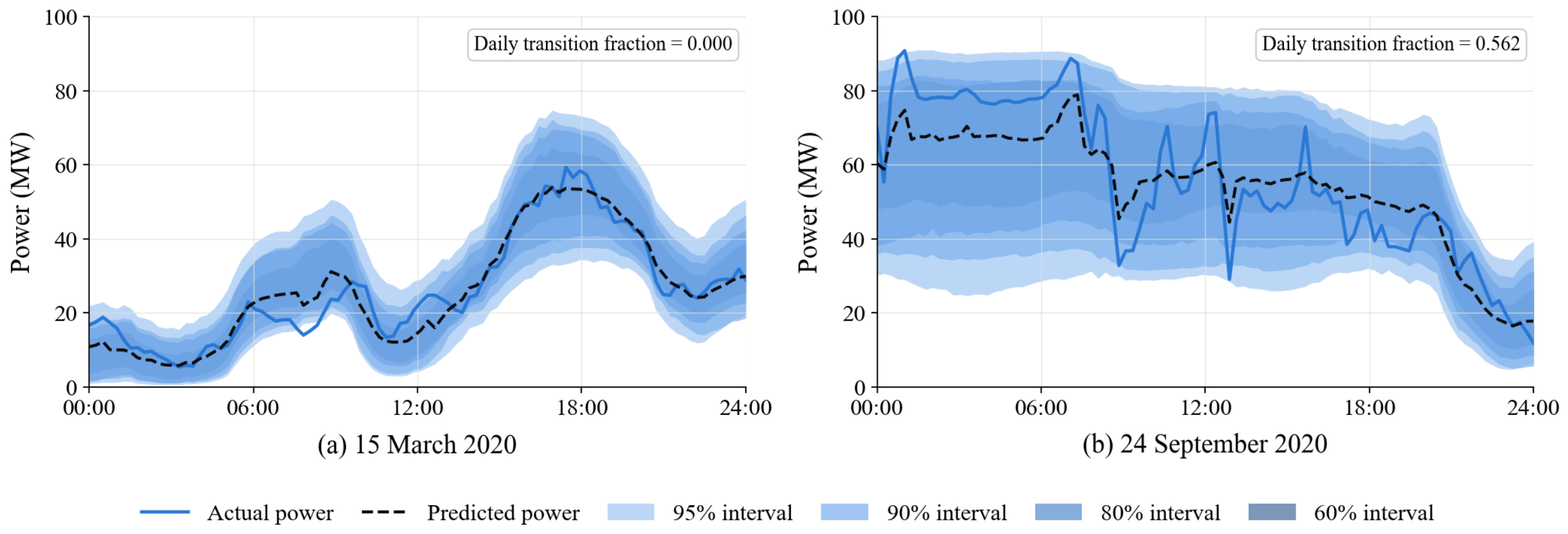
To demonstrate forecasting performance under different weather types more intuitively, Figure 6 presents the forecasts for a conventional-weather day (15 March 2020) and a transitional-weather day (24 September 2020). On the conventional-weather day, the power curve varies relatively smoothly, and the point forecast captures most power fluctuations, with relatively compact prediction intervals. On the transitional-weather day, power fluctuations are larger. Although the point forecast follows the overall power trend, it exhibits a relatively large error at the peak. The prediction intervals are wider than those on the conventional-weather day, adapting to the increased uncertainty during the transitional period.
Figure 6.
One-day forecasting results for different weather types.
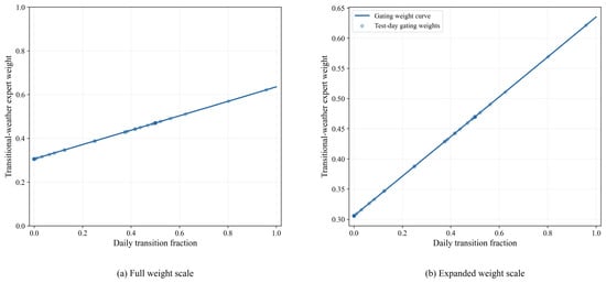
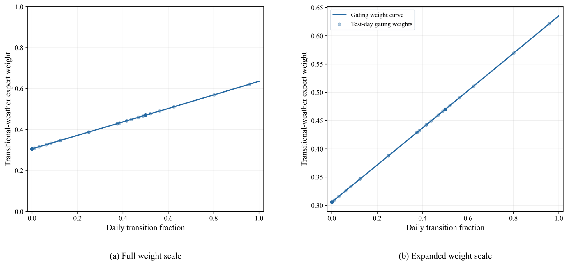
Figure 7 illustrates the relationship between the daily transition fraction and the fusion weight assigned to the transitional-weather expert. The solid line represents the learned gating function, while the scatter points indicate the corresponding weights for the test days. The two subplots display the weights on the full scale and a locally enlarged scale, respectively. Within the displayed range, the weight assigned to the transitional-weather expert increases with the daily transition fraction, rising from approximately 0.31 to 0.63. This indicates that the model increases the relative contribution of this branch when transitional-weather conditions account for a larger proportion of the forecast day. Meanwhile, the weights do not approach either 0 or 1, indicating that both branches retain a certain degree of contribution.
Figure 7.
Relationship between gating weights and daily transition fraction.
3.6. Parameter Sensitivity Analysis
To evaluate the robustness of the proposed model to hyperparameter selection, one-factor-at-a-time sensitivity analyses are conducted from three perspectives: model architecture and regularization, transitional-weather identification, and expert gating. Specifically, six parameters are investigated: the model dimension , dropout rate, transition identification threshold , sliding window length L, one-sided extension length H, and entropy regularization coefficient .
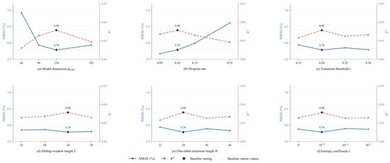
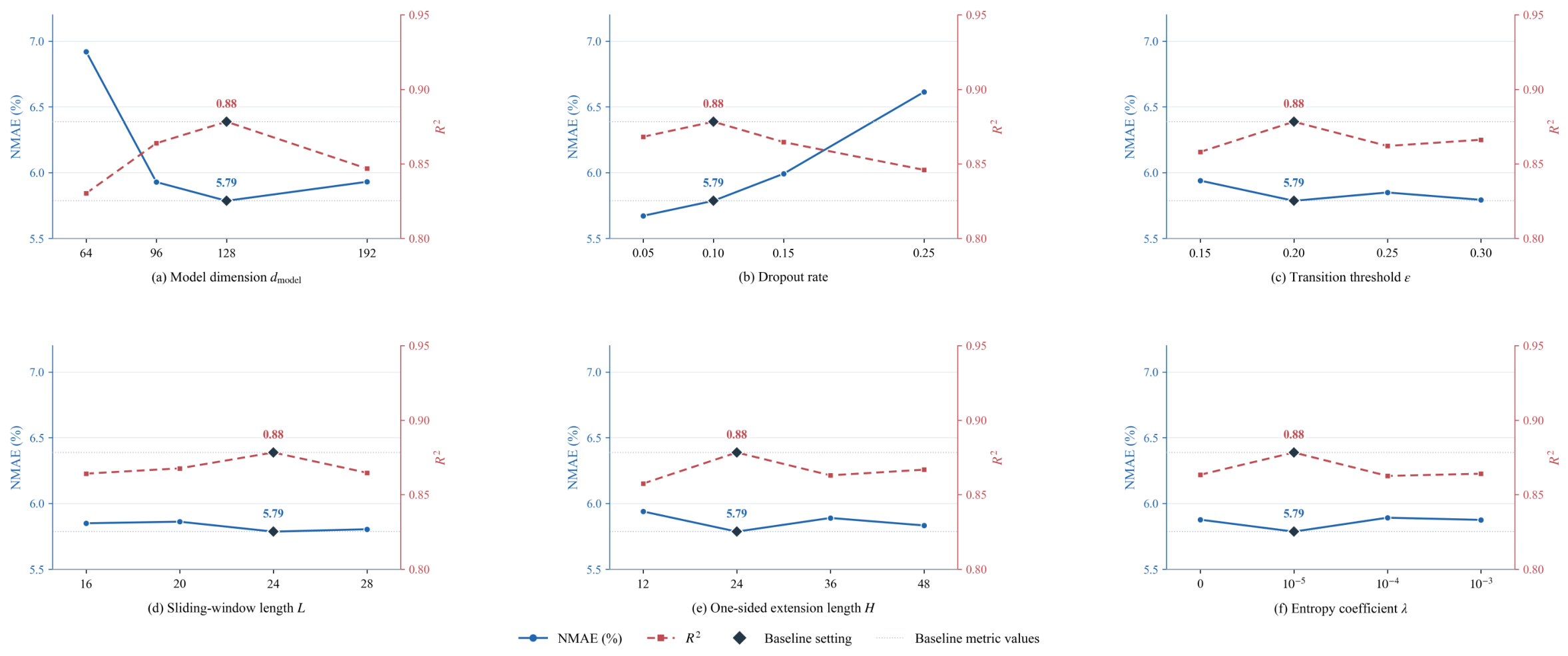
Table 6 shows that, within the examined parameter ranges, has the greatest impact on point forecasting performance. Reducing it from 128 to 64 increases NMAE from 5.79% to 6.92% and decreases from 0.88 to 0.83, suggesting limited feature representation at smaller dimensions. At 96 or 192, NMAE is 5.93%, slightly above the baseline. Increasing the Dropout rate from 0.05 to 0.25 raises NMAE from 5.68% to 6.61% and lowers from 0.87 to 0.85, suggesting that excessive dropout may impair the fitting of meteorological–power relationships. In contrast, changes to the transition detection and gating parameters have relatively small effects on point forecasting performance within the examined ranges. Figure 8 visualizes these parameter-dependent changes.
Table 6.
Forecasting results under different parameter settings.
Figure 8.
Parameter sensitivity results.
The baseline configuration is not optimal across all metrics: a Dropout rate of 0.05 yields a lower NMAE than the baseline, but a lower . Parameter selection should therefore consider both error reduction and the ability to explain power variations.
3.7. Ablation Study
To verify the contributions of the modules in the proposed model, ablation experiments are conducted. The experiments focus on three core modules: the transitional-weather identification module (Trans), the cross-attention decoder (CA), and the mixture-of-experts network (MoE). The complete model is denoted as A0, and five additional ablation configurations are denoted as A1–A5. Specifically, A1 removes MoE, A2 replaces the cross-attention branch with a concatenation-based MLP that retains stepwise encodings and global context, A3 removes transition information, A4 removes both MoE and transition information, and A5 removes all three modules.
The ablation results in Table 7 show that MoE mainly improves forecasting accuracy and interval sharpness. Removing MoE raises overall NMAE from 5.79% to 6.52%, with a 12.75% relative increase on transitional weather days, indicating that the dual-expert structure better captures power variations across weather conditions. On transitional-weather days, removing MoE increases PINAW from 0.33 to 0.38 while lowering PICP from 94.33% to 93.75%. CWC and NIS increase from 0.70 to 1.08 and from 0.45 to 0.48, respectively, indicating poorer interval quality despite the wider intervals.
Table 7.
Ablation study results.
Cross-attention and transition information support information fusion and weather-state guidance, respectively. Replacing cross-attention with a concatenation-based MLP raises NMAE to 6.08%, while NIS decreases slightly from 0.38 to 0.37. This indicates a loss of point-forecasting accuracy, although interval quality does not deteriorate according to NIS. Removing transition information narrows the intervals on transitional-weather days, with PINAW decreasing from 0.33 to 0.31, but lowers PICP from 94.33% to 90.80%. CWC increases from 0.70 to 2.87, and NIS rises from 0.45 to 0.52. These results indicate that transition information improves the balance between interval coverage and width.
Removing both MoE and transition information requires wider intervals to maintain coverage. Removing all three modules raises NMAE to 12.45% and lowers to 0.50, demonstrating their combined contribution. The full model achieves a better balance among forecasting accuracy, interval coverage, and interval sharpness.
4. Discussion and Conclusions
4.1. Discussion
Weather transition detection in this study relies on NWP wind speed and temperature forecasts. Errors in their timing and magnitude may lead to misidentified transition periods and affect power forecasts through the masks and meteorological inputs. Although wind direction, air pressure, and other variables are used in downstream forecasting, they are not included in the transition detection criteria. Future work could assess detection robustness through forecast perturbation and variable combination experiments. Expert fusion uses daily gating. Although stepwise masks indicate intraday transition locations, the fusion weights shared throughout the day cannot readily adapt to local weather changes. Stepwise gating could therefore be explored to improve intraday adaptability.
Some prediction intervals remain undercovered during transitional weather. Adding representative transition samples and applying conditional calibration by weather type or daily transition fraction on an independent calibration set could improve the balance between coverage and interval width. Validation is limited to a single wind farm, so the generalizability of the findings is constrained by site conditions and the sampling period. Data from multiple wind farms and years are needed to assess the transferability of the transition detection parameters and forecasting model.
4.2. Conclusions
To address the limited forecasting accuracy of wind power under transitional weather conditions, a transition-aware day-ahead probabilistic wind power forecasting method based on a mixture-of-experts network is proposed. The method is developed from three complementary components: weather-state identification, temporal dependency modeling, and adaptive uncertainty quantification. Validation using measured data from a wind farm leads to the following conclusions:
- (1)
- The transitional-weather identification process provides explicit meteorological change information through a transition mask. Ablation results show that incorporating this information improves forecasting accuracy and the balance between prediction interval coverage and width, particularly on transitional-weather days.
- (2)
- The proposed framework improves both point and probabilistic wind power forecasting performance. The point-forecasting NMAE is 5.79%, corresponding to a 4.61–31.88% reduction relative to the baseline models. The CWC of the 95% prediction interval is 21.36% lower than that of the baseline with the lowest mean CWC.
- (3)
- The dynamic fusion mechanism of the MoE adjusts the forecasting strategy according to different weather states, improving forecasting accuracy and uncertainty quantification under transitional weather. The model achieves an NMAE of 6.90% on transitional-weather days, which is 11.31% lower than that of the model without the MoE network. Across the four nominal coverage levels, prediction intervals on transitional-weather days are approximately 10.00–16.67% wider than those on conventional-weather days.
Author Contributions
Conceptualization, W.S. and Y.W.; methodology, W.S. and J.H.; software, J.H.; validation, Y.W., Y.D. and S.H.; formal analysis, J.H.; investigation, Y.D.; resources, S.Y.; data curation, J.H.; writing—original draft preparation, J.H.; writing—review and editing, W.S., Y.W. and S.H.; visualization, J.H.; supervision, W.S.; project administration, Y.W.; funding acquisition, Y.W. All authors have read and agreed to the published version of the manuscript.
Funding
This research was supported by the China Huaneng Group Technology Project (HNKJ24-H130).
Data Availability Statement
The data presented in this study are available on request from the corresponding author.
Acknowledgments
The authors thank those who provided valuable comments and suggestions on this manuscript.
Conflicts of Interest
Authors Yimei Wang and Yifei Dou were employed by the company Huaneng Clean Energy Research Institute (CERI). Author Shaoyi Yang was employed by the company Hebei Hanfeng Power Generation Co., Ltd. The remaining authors declare that the research was conducted in the absence of any commercial or financial relationships that could be construed as a potential conflict of interest. The authors declare that this study was supported by China Huaneng Group Technology Project (HNKJ24-H130). The funder had the following involvement with the study: manuscript review during the writing stage and approval of the submission of this article.
Abbreviations
The following abbreviations are used in this manuscript:
| NWP | Numerical Weather Prediction |
| WSMSF | Wind Speed Mutation Sensitivity Factor |
| EMA | Exponential Moving Average |
| MLP | Multilayer Perceptron |
| CNN | Convolutional Neural Network |
| LSTM | Long Short-Term Memory |
| BiLSTM | Bidirectional Long Short-Term Memory |
| GAN | Generative Adversarial Network |
| MoE | Mixture-of-Experts |
| SDA | Swinging Door Algorithm |
| SCRF | Semi-supervised Contrastive Regression Framework |
| LightGBM | Light Gradient Boosting Machine |
| RF | Random Forest |
| NMAE | Normalized Mean Absolute Error |
| PICP | Prediction Interval Coverage Probability |
| PINAW | Prediction Interval Normalized Average Width |
| CWC | Coverage Width-based Criterion |
| NIS | Normalized Interval Score |
| AdamW | Adam with Decoupled Weight Decay |
References
- Wang, B.; Feng, S.L.; Liu, X.L.; Wang, Z. Short-Term Wind Power Forecasting Considering Transitional Weather Process Identification and Verification. South. Power Syst. Technol. 2023, 17, 52–62. [Google Scholar] [CrossRef]
- Cui, Y.; Chen, Z.; He, Y.; Xiong, X.; Li, F. An Algorithm for Forecasting Day-Ahead Wind Power via Novel Long Short-Term Memory and Wind Power Ramp Events. Energy 2023, 263, 125888. [Google Scholar] [CrossRef] [Scilit]
- Sun, R.F.; Zhang, T.; He, Q.; Xu, H.X. A Review of Key Technologies and Applications of Wind Power Forecasting. High Volt. Eng. 2021, 47, 1129–1143. [Google Scholar] [CrossRef]
- Zhang, D.Y.; Dai, Y.; Zhang, X.; Zhang, J.; Wang, Z.C.; Xue, L. Review and Prospect of Wind Power Ramp Event Research. Power Syst. Technol. 2018, 42, 1783–1792. [Google Scholar] [CrossRef]
- Liu, Y.T.; Yang, M.; Yu, Y.X.; Li, M.L.; Wang, B. Day-Ahead Wind Power Forecasting for Transitional Weather Based on Multi-Scenario Sensitive Meteorological Factor Selection and Small-Sample Learning and Augmentation. High Volt. Eng. 2023, 49, 2972–2982. [Google Scholar] [CrossRef]
- Ye, L.; Pei, M.; Yang, J.B.; Song, X.R.; Luo, Y.D.; Zhang, Z.Y.; Yu, Y.J.; Tang, Y. Power and Energy Balance System of Renewable Energy Power System under Extreme Weather. Autom. Electr. Power Syst. 2025, 49, 2–18. [Google Scholar]
- Zhang, Z.Y.; Lan, L.; Bai, J.S.; Yang, T.Y.G.; Kong, H.; Liu, H. Research on Wind Power Forecasting Methods under Small-Sample Conditions. Power Syst. Prot. Control 2025, 53, 120–130. [Google Scholar]
- Ran, H.J.; Yang, J.F.; Dong, J.H.; Huang, X. Short-Term Wind Power Scenario Generation Method Based on Combined Forecasting Models. Mod. Electron. Tech. 2026, 49, 114–120. [Google Scholar] [CrossRef]
- Fujimoto, Y.; Takahashi, Y.; Hayashi, Y. Alerting to Rare Large-Scale Ramp Events in Wind Power Generation. IEEE Trans. Sustain. Energy 2019, 10, 55–65. [Google Scholar] [CrossRef] [Scilit]
- Ren, G.; Wan, J.; Wang, Y.; Yao, K.; Fu, J.; Yu, J. A Direct Prediction Method for Wind Power Ramp Events Considering the Class Imbalanced Problem. Energy Sci. Eng. 2023, 11, 1705–1715. [Google Scholar] [CrossRef] [Scilit]
- Zhou, B.; Duan, H.; Wu, Q.; Wang, H.; Or, S.W.; Chan, K.W.; Meng, Y. Short-Term Prediction of Wind Power and Its Ramp Events Based on Semi-Supervised Generative Adversarial Network. Int. J. Electr. Power Energy Syst. 2021, 125, 106411. [Google Scholar] [CrossRef] [Scilit]
- Meng, A.; Chen, S.; Ou, Z.; Xiao, J.; Zhang, J.; Chen, S.; Zhang, Z.; Liang, R.; Zhang, Z.; Xian, Z.; et al. A Novel Few-Shot Learning Approach for Wind Power Prediction Applying Secondary Evolutionary Generative Adversarial Network. Energy 2022, 261, 125276. [Google Scholar] [CrossRef] [Scilit]
- Meng, A.; Zhang, H.; Yin, H.; Xian, Z.; Chen, S.; Zhu, Z.; Zhang, Z.; Rong, J.; Li, C.; Wang, C.; et al. A Novel Multi-Gradient Evolutionary Deep Learning Approach for Few-Shot Wind Power Prediction Using Time-Series GAN. Energy 2023, 283, 129139. [Google Scholar] [CrossRef] [Scilit]
- Xu, C.; Cui, S.; Wei, L.; Zhu, B.; Ai, X.; Fang, J.; Wen, J. Wind Power Forecasting Under Extreme Weather: A Novel Few-Shot Learning Architecture. IEEE Trans. Sustain. Energy 2026, 17, 788–803. [Google Scholar] [CrossRef] [Scilit]
- Li, Y.J.; Chen, F.H.; Yan, J.; Ge, C.; Han, S.; Liu, Y.Q. Extreme Weather Adaptive Short-Term Wind Power Forecasting Based on Transfer Learning and Autoencoder. Autom. Electr. Power Syst. 2025, 49, 85–95. [Google Scholar] [CrossRef]
- Wang, E.R.; Su, X.J.; Gong, J.H.; Liu, Z.Y.; Fu, Y. Typhoon-Oriented Offshore Wind Power Ramp Event Prediction Method. Zhejiang Electr. Power 2026, 45, 80–90. [Google Scholar] [CrossRef]
- Liang, Z.; Zhang, Z.; Shi, Y.; Liu, L. Identification Method and Characteristic Analysis of Wind Speed and Wind Power Ramp Events Based on Swinging Door Algorithm. J. Univ. Chin. Acad. Sci. 2024, 41, 821–829. [Google Scholar]
- Lochmann, M.; Kalesse-Los, H.; Schäfer, M.; Heinrich, I.; Leinweber, R. Analysing Wind Power Ramp Events and Improving Very Short-Term Wind Power Predictions by Including Wind Speed Observations. Wind Energy 2023, 26, 573–588. [Google Scholar] [CrossRef] [Scilit]
- Xiong, Y.H.; Peng, X.S.; Yang, Z.M.; Wei, P.J.; Deng, W.S.; Dai, Z.F. Wind Power Ramp Event Identification Based on Parameter-Adaptive Swinging Door and Bump Event Screening. South. Power Syst. Technol. 2023, 17, 101–110. [Google Scholar]
- Cui, Y.; He, Y.; Xiong, X.; Chen, Z.; Li, F.; Xu, T.; Zhang, F. Algorithm for Identifying Wind Power Ramp Events via Novel Improved Dynamic Swinging Door. Renew. Energy 2021, 171, 542–556. [Google Scholar] [CrossRef] [Scilit]
- Song, W.; Yan, J.; Han, S.; Liu, S.; Wang, H.; Dai, Q.; Huo, X.; Liu, Y. A Multi-Task Spatio-Temporal Fusion Network for Offshore Wind Power Ramp Events Forecasting. Renew. Energy 2024, 237, 121774. [Google Scholar] [CrossRef] [Scilit]
- Yu, G.Z.; Lu, L.; Tang, B.; Wang, S.Y.; Chung, C.Y. Ultra-Short-Term Wind Power Subsection Forecasting Method Based on Extreme Weather. IEEE Trans. Power Syst. 2023, 38, 5045–5056. [Google Scholar] [CrossRef] [Scilit]
- Lyners, D.; Vermeulen, H.; Groch, M. Wind Power Ramp Event Detection Using a Multi-Parameter Segmentation Algorithm. Energy Rep. 2021, 7, 5536–5548. [Google Scholar] [CrossRef] [Scilit]
- Jing, H.T.; Han, L.; Gao, Z.Y. Wind Power Ramp Prediction Based on Convolutional Neural Network Feature Extraction. Autom. Electr. Power Syst. 2021, 45, 98–105. [Google Scholar] [CrossRef]
- Zhu, N.; Dai, Z.; Wang, Y.; Zhang, K. A Contrastive Learning-Based Framework for Wind Power Forecast. Expert Syst. Appl. 2023, 230, 120619. [Google Scholar] [CrossRef] [Scilit]
- Couto, A.; Estanqueiro, A. Enhancing Wind Power Forecast Accuracy Using the Weather Research and Forecasting Numerical Model-Based Features and Artificial Neuronal Networks. Renew. Energy 2022, 201, 1076–1085. [Google Scholar] [CrossRef] [Scilit]
- Resen, A.K.; Khamees, A.B.; Yaseen, S.F. Determination of Wind Shear Coefficients and Conditions of Atmospheric Stability for Three Iraqi Sites. IOP Conf. Ser. Mater. Sci. Eng. 2020, 881, 012161. [Google Scholar] [CrossRef] [Scilit]
- Okada, M.; Yamaguchi, K.; Kodama, R.; Ogasawara, N.; Kato, H.; Doan, V.Q.; Ishizaki, N.N.; Kusaka, H. Development of a Wind Power Ramp Forecasting System via Meteorological Pattern Analysis. Wind Energy 2022, 25, 1900–1916. [Google Scholar] [CrossRef] [Scilit]
- Michalakopoulos, V.; Zakynthinos, A.; Sarmas, E.; Marinakis, V.; Askounis, D. Hybrid Short-Term Wind Power Forecasting Model Using Theoretical Power Curves and Temporal Fusion Transformers. Renew. Energy 2026, 256, 124008. [Google Scholar] [CrossRef] [Scilit]
- Yu, G.Z.; Lu, L.; Tang, B.; Wang, S.Y.; Dong, Q. Ultra-Short-Term Subsection Forecasting Method for Offshore Wind Power Considering Transitional Weather. Proc. CSEE 2022, 42, 4859–4870. [Google Scholar] [CrossRef]
- Hu, J.; Luo, Q.; Tang, J.; Heng, J.; Deng, Y. Conformalized Temporal Convolutional Quantile Regression Networks for Wind Power Interval Forecasting. Energy 2022, 248, 123497. [Google Scholar] [CrossRef] [Scilit]
- Shi, S.; Zhang, H.; Huang, D.M.; Li, Y.Y.; Mi, Y.; Yang, X.D. Short-Term Zonal Power Prediction of Offshore Wind Power Considering Ramp Characteristics. Acta Energiae Solaris Sin. 2024, 45, 258–268. [Google Scholar] [CrossRef]
- Cui, Y.; Cheng, C.; Zhu, Y.; Meng, D.; Chen, Z. A Novel Two-Step Framework for Day-Ahead Wind Power Probabilistic Forecasting Considering Uncertainties and Ramp Events. Int. J. Electr. Power Energy Syst. 2025, 169, 110780. [Google Scholar] [CrossRef] [Scilit]
- Zhang, W.; Sun, H.; Gao, J.; Yan, G.; Yang, M. A Two-Stage Ultra-Short-Term Wind Power Forecasting Method Based on Transitional Weather Identification and Meteorological Prediction Error Propagation. IEEE Trans. Sustain. Energy 2026, 17, 295–306. [Google Scholar] [CrossRef] [Scilit]

Disclaimer/Publisher’s Note: The statements, opinions and data contained in all publications are solely those of the individual author(s) and contributor(s) and not of MDPI and/or the editor(s). MDPI and/or the editor(s) disclaim responsibility for any injury to people or property resulting from any ideas, methods, instructions or products referred to in the content. |
© 2026 by the authors. Licensee MDPI, Basel, Switzerland. This article is an open access article distributed under the terms and conditions of the Creative Commons Attribution (CC BY) license.