IGWO- and LSTM-Based Fault Diagnosis for Gear Transmission Systems in Mining Equipment

Abstract

Large-scale mining excavators often operate under complex and variable working conditions, making the transmission system susceptible to non-stationary vibration signals, substantial environmental noise, and weak early-fault features. To address these challenges, this study proposes a fault diagnosis method that integrates vibration-signal processing, improved Grey Wolf Optimization, long short-term memory (LSTM) networks. First, the raw vibration signals are decomposed using the complete ensemble empirical mode decomposition with adaptive noise (CEEMDAN) method. A hybrid screening strategy based on Pearson correlation coefficients and Shannon entropy is then employed to identify informative intrinsic mode functions and reconstruct the vibration signals, thereby suppressing noise and enhancing fault-related features. Subsequently, an improved Grey Wolf Optimization (IGWO) algorithm is developed by introducing an adaptive convergence-factor adjustment mechanism and a dynamic weighting strategy for position updating, which improves the algorithm’s global exploration capability and local exploitation accuracy. The IGWO algorithm is further used to optimize the key parameters of an LSTM network, resulting in a CEEMDAN–IGWO–LSTM fault-diagnosis model for identifying different operating and fault conditions of the transmission system. The experimental results show that the proposed denoising method outperforms moving-average filtering and the least-mean-square algorithm in preserving and enhancing fault-related vibration features. The optimized LSTM model achieves average diagnostic accuracies of 96.87%, 97.86%, 96.79%, and 96.67% for the four test datasets, respectively, representing improvements of 10.17, 5.26, 6.99, and 9.07 percentage points over the unoptimized one-dimensional LSTM model. Moreover, compared with the deep-learning-based VMD–DBN method, the proposed approach achieves a further 2.21% improvement in diagnostic accuracy. The results demonstrate that the proposed method can effectively improve the accuracy and robustness of fault diagnosis and provide a reliable technical basis for condition monitoring and predictive maintenance of transmission systems in large-scale mining excavators.

1. Introduction

Gear transmission systems, as critical components of large-scale mining machinery, directly impact equipment operation when failures occur. Modern fault diagnosis techniques, underpinned by advanced sensing technologies and reliability theory, have spawned numerous diagnostic methods for gear transmission systems. These include noise analysis and vibration monitoring, torsional vibration analysis, oil analysis, acoustic emission, and temperature and energy consumption monitoring [1]. Among these, vibration diagnosis stands as a widely adopted and highly effective fault detection method, finding extensive application both domestically and internationally. During mechanical operation, components within the gearbox such as gears, bearings, and shafts generate characteristic vibrations. By collecting and analysing the vibration signals produced by these components during operation, their operational status can be determined.

The harsh operating environment and severe background noise of heavy mining equipment, coupled with the complex structure of gear transmission systems and diverse vibration signal transmission pathways, result in highly complex vibration signal components. This poses significant challenges for diagnosing gear transmission systems. During fault identification, analysing and extracting features from raw vibration signals is essential. This paper monitors vibration signals generated during gear transmission system operation, extracts signals from each operational phase, applies noise reduction processing, and then extracts key feature data. This feature data is subsequently input into a fault model to ultimately identify and analyse the operational status of the gear transmission system [2], thereby locating the position of component faults.

2. Vibration Characteristics and Problem Definition of Gear Transmission Systems

Vibration signals in gear transmission systems collectively encompass the vibration responses and radiated acoustic noise generated during system operation. The acoustic characteristics of these signals vary considerably with the working environment, and based on the features of noise signals under different operating conditions, the associated noise in such systems can be categorized into three distinct types: high-frequency random noise, low-frequency random noise, and high-frequency discrete noise. High-frequency random noise arises primarily from contact friction and meshing impacts during gear engagement. Low-frequency random noise is mainly induced by structural imperfections such as tooth surface wear and assembly clearances. High-frequency discrete noise, in turn, stems principally from the vibration-driven agitation of internal gearbox media, including lubricating oil, air, and aqueous fluids.

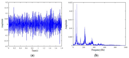
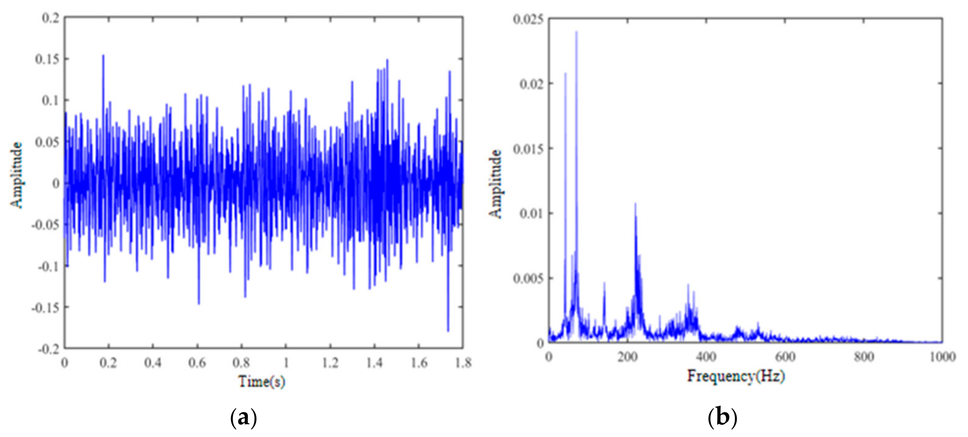
At underground fully mechanized longwall mining faces, vibration signals acquired by sensors are severely contaminated by complex background noise, rendering the effective vibration signals emanating from mechanical operations highly prone to being masked by intense ambient noise. Vibration excitations induced by the operation of gear transmission systems are predominantly manifested in both radial and axial directions. Furthermore, the lubricating oil enclosed within the housing of transmission components exerts a non-negligible influence on the propagation characteristics of gear-induced vibration signals. Additionally, vibrations transmitted from the base of the transmission system introduce extraneous noise interference, which further exacerbates the difficulty of extracting effective vibration signals. Figure 1 depicts the time-domain waveform of a vibration signal segment collected from an online monitoring test rig for a gear transmission system. As is evident from the figure, significant background noise causes the original effective vibration signal to be rapidly obscured.

Figure 1. Vibration signal of the laboratory bench gearbox: (a) time-domain signal; (b) frequency-domain signal.

The current dataset contains labeled samples collected under several healthy and faulty operating conditions, but it does not provide complete run-to-failure degradation trajectories. Consequently, the present experiments validate fault-state classification rather than time-to-failure prediction or fully validated early fault diagnosis. The absence of continuous degradation labels also limits the direct estimation of warning lead time. This limitation will be addressed in future work by collecting long-term degradation data and defining an experimentally validated incipient-fault stage.

Considering the non-stationary, impulsive, and noise-contaminated characteristics of gear transmission vibration signals, this study focuses on three problems. First, effective components related to early faults must be extracted from raw vibration signals containing environmental noise and operational impacts. Second, a fault-classification model with good generalization must be established under different loads and operating conditions. Third, the dependence of the key LSTM parameters on manual experience must be reduced in order to improve convergence and classification stability.

To address these problems, the raw vibration signals are first decomposed adaptively using CEEMDAN. Informative intrinsic mode functions are then selected and reconstructed using Pearson correlation coefficients and Shannon entropy. Time-domain, frequency-domain, and statistical features are subsequently extracted and provided to an LSTM network optimized by IGWO for the identification of different transmission-system conditions. Section 2 is intended to describe the signal characteristics, noise sources, and research problem, whereas Section 3 provides the detailed decomposition, optimization, and classification methodology.

3. Algorithms and Neural Network Research

3.1. CEEMDAN Noise Reduction Algorithm

The joint denoising algorithm for modal preference reconstruction and representation aims to enhance information reconstruction and expression by integrating data from different modalities [3], while simultaneously mitigating the impact of noise. Within fault diagnosis systems, multiple sensor types are typically deployed to monitor equipment status, including vibration sensors, temperature sensors, and acoustic sensors. The data generated by these sensors is multimodal, encompassing diverse forms and properties [4]. Consequently, preprocessing of this raw data is essential, involving outlier removal, standardisation, and normalisation to prepare it for subsequent analysis. Within multimodal datasets, modality data most suitable for reconstruction and representation purposes is selected based on each modality’s quality and relevance. Subsequently, algorithmic optimisation reconstructs the chosen modality data [5,6] to enhance data quality, including clarity and precision. Furthermore, the representation of data is refined to better suit subsequent processing or analysis. This is achieved through techniques such as dimensionality reduction and feature extraction, combined with multiple noise reduction methods. These approaches mitigate noise at various levels to yield more accurate results.

Although CEEMDAN can adaptively decompose non-stationary vibration signals and alleviate mode mixing to some extent, the use of CEEMDAN alone still has several limitations. First, the decomposition results are affected by parameters such as the noise amplitude, ensemble size, and stopping criterion. When the raw signal contains strong environmental noise or multiple fault-related frequency components, some intrinsic mode functions may simultaneously contain fault impulses and noise components, which can affect the subsequent feature extraction process. Second, conventional CEEMDAN-based methods generally select informative modes according to the correlation coefficient, energy, or manually defined empirical thresholds. This introduces a certain degree of dependence on prior experience and may not provide stable results under different rotational speeds, loads, and noise conditions. Therefore, CEEMDAN alone may be insufficient for extracting weak fault features and achieving adaptive diagnosis under complex operating conditions.

The steps for signal decomposition using CEEMDAN are as follows:

(1)

Let the original signal be $x(t)$. Add Gaussian white noise with a standard deviation of ${\epsilon }_0$ to the original signal I times, forming I noisy sequences:

$$x_i(t)=x(t)+{\epsilon }_0{n}_i(t)\hspace{1em}(i=1,2\dots ,I)$$

(1)

(2)

For each noise-added sequence $x(t)$, performing EMD yields the following first-order modal components from the CEEMDAN decomposition:

$$c_1(t)={\displaystyle \frac{1}{I}}{\displaystyle \sum _{i=1}^I{c}_{i1}}(t)$$

(2)

The first residual component obtained is

$$r_1(t)=x(t)-c_1(t)$$

(3)

In the formula, $c_{i1}(t)$ denotes the first-order modal component obtained by decomposing each noise sequence $x_i(t)$.

(3)

Continue adding I instances of adaptive Gaussian white noise ${\epsilon }_1{E}_1(n_i(t))$ to the residual component $r_1(t)$, forming I noise-added sequences, namely:

$$r_{1i}(t)=r_1(t)+{\epsilon }_1{E}_1\left(n_i(t)\right)$$

(4)

(4)

Performing EMD on $r_{1i}(t)$ yields the second-order modal component $c_2(t)$ from the CEEMDAN decomposition as follows:

$$c_2(t)={\displaystyle \frac{1}{I}}{\displaystyle \sum _{i=1}^I{E}_1}\left[r_i(t)+{\epsilon }_1{E}_1\left(n_i(t)\right)\right]$$

(5)

(5)

Repeat steps (3) and (4) to obtain the $k+1$th-order modal component and the $k$th residual component, namely

$$c_{k+1}(t)={\displaystyle \frac{1}{I}}{\displaystyle \sum _{i=1}^I{E}_1}\left[r_k(t)+{\epsilon }_k{E}_k\left(n_i(t)\right)\right]$$

(6)

$$r_k(t)=r_{k-1}(t)+c_k(t)$$

(7)

(6)

Repeat step (5) until no more than two residual signal extrema points are obtained. The final residual components are

$$r(t)=x(t)-{\displaystyle \sum _{k=1}^K{c}_k}(t)$$

(8)

Following decomposition by the CEEMDAN method, the original vibration signal sequence is decomposed into the sum of IMF components and residual components:

$$x(t)=r(t)+{\displaystyle \sum _{k=1}^K{c}_k}(t)$$

(9)

CEEMDAN decomposition facilitates the separation of valid vibration signals from environmental noise interferences. In this study, a strategy for selecting optimal intrinsic mode function (IMF) components for feature extraction is proposed, which employs a hybrid screening criterion integrating Pearson correlation coefficients and the Shannon entropy criterion, based on the intrinsic characteristics of vibration signals and interference noise.

The Pearson correlation coefficient, also known as the Pearson product-moment correlation coefficient, is a statistical measure used to quantify the degree of linear correlation between two variables X and Y [7]. Its value ranges between −1 and 1. The correlation coefficient criterion is employed to analyse the degree of correlation between the IMF and the original vibration signal. A higher correlation coefficient indicates that the IMF contains more characteristic information from the original vibration signal, whereas a lower coefficient suggests the IMF contains more noise and irrelevant components. The expression for the correlation degree between the IMF and the original vibration signal is

$$R_{X{C}_i}={\displaystyle \frac{{\displaystyle \sum _{t=1}^N[x(t)-\overline{x(t)}}][c_i(t)-\overline{c_i(t)}]}{\sqrt{{\displaystyle \sum _{t=1}^N{[x(t)-\overline{x(t)}]}^2{[c_i(t)-\overline{c_i(t)}]}^2}}}}$$

(10)

In the equation, $R_{x{c}_i}$ denotes the correlation coefficient between the $i$th IMF and the original signal $x(t)$; $t=1,2,\dots N$ represents the sampling point of the signal.

It is generally accepted that 1 indicates a perfect positive correlation, values between 0.1 and 0.5 denote a weak correlation, and −1 signifies a perfect negative correlation. Based on the correlation coefficient screening criterion, this study directly discarded the IMF showing a weak correlation with the original vibration signal. Subsequently, Shannon entropy was employed to conduct a secondary screening of the remaining IMFs.

For signals exhibiting pronounced vibration within gear transmission systems, where the amplitude of the original sequence exceeds that of background noise, applying the correlation coefficient criterion to filter the decomposed IMF components can effectively eliminate irrelevant elements. Conversely, for signals with weak vibrations, background noise constitutes the primary component. Relying solely on the correlation coefficient criterion for signal filtering reduces accuracy, making it highly susceptible to extracting useless noise signals and consequently compromising the quality of signal reconstruction.

Shannon entropy, proposed by Claude Shannon in information theory, serves as a measure of the uncertainty inherent in information [8]. It reflects the average information content, or degree of uncertainty, within a given set of data. When all possible events occur with equal probability, the entropy of the information reaches its maximum value. Its expression is as follows:

$$H(X)=-{\displaystyle \sum _{i=1}^{n}P}\left(x_i\right)\log P\left(x_i\right)$$

(11)

In the formula, $P\left(x_i\right)$ denotes the probability that the variable takes the specific value $x_i$, $X$ is a discrete random variable, $n$ is the total number of possible values $X$ can assume, and $b$ is the base of the logarithm, typically taken as 2, though it may also be taken as the base of the natural logarithm, $e$.

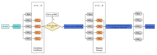
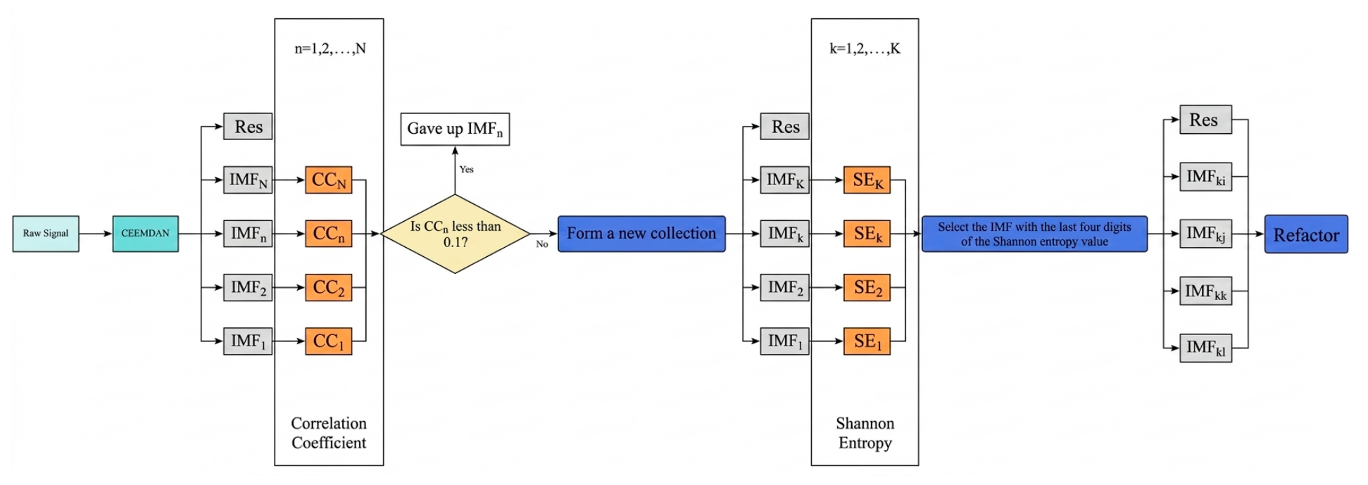
Shannon entropy reflects the amount of information carried by a data segment. An IMF with a higher proportion of noise and less effective information carries greater disorder, and thus exhibits higher Shannon entropy, whereas the IMF characterising a vibration signal is a non-stationary random signal. At the instant of a vibration impact, it exhibits abrupt changes in amplitude within the time domain. It contains more vibration fault feature information and exhibits more pronounced vibration characteristics. Compared to noise-dominated IMFs, its degree of disorder is lower, resulting in a smaller Shannon entropy. This study proposes selecting the four IMF components with the lowest Shannon entropy rankings from the newly generated IMF set for reconstruction. The overall workflow is illustrated in Figure 2.

Figure 2. Flowchart of the CEEMDAN noise reduction algorithm.

3.2. Improvements to the Grey Wolf Optimisation Algorithm

To overcome the limitations of the standard GWO—namely poor population diversity, slow convergence in the later stage, and susceptibility to local optima—this study proposes three modifications: (1) chaotic-mapping-based population initialization, (2) a quadrantal-ellipse convergence-parameter update strategy, and (3) an adaptive dynamic-weight position update strategy. Each modification is described below, together with the specific deficiency of the standard GWO that it addresses and its expected effect on the balance between global exploration and local exploitation.

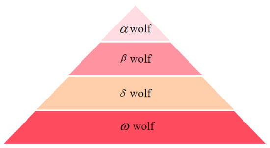
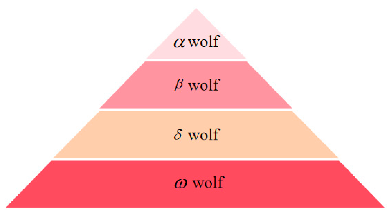
The Grey Wolf Optimisation Algorithm is a swarm intelligence optimisation technique proposed by Mirjalili et al. from Griffith University, Australia, in 2014 [9]. This algorithm draws inspiration from the predatory behaviour of grey wolf packs, simulating their leadership hierarchy and hunting mechanisms. Within the algorithm, wolves are categorised into four distinct types to represent hierarchical levels: the alpha wolf (α), responsible for directing search efforts; the beta wolf (β) and delta wolf (δ), who assist the alpha wolf; and the omega wolves (ω), tasked with executing the majority of search activities. The structural framework is illustrated in Figure 3.

Figure 3. Schematic diagram of grey wolf population hierarchy.

The Grey Wolf Algorithm’s search process comprises two phases: exploration and exploitation. During the exploration phase, the grey wolves deviate from the prey using random values to conduct a global search. In the exploitation phase, the wolves concentrate their search around the prey—that is, the mathematical model representing potential solutions to the optimisation problem. This model defines the wolves’ next position by considering the locations of the lead wolf, the second lead wolf, and the third lead wolf [10].

The hunting process of grey wolf populations can be described by the following mathematical model:

$$D=\left|C\cdot X_p(t)-X(t)\right|$$

(12)

$$X(t+1)=X_p(t)-A\cdot D$$

(13)

where $D$ denotes the distance vector between the grey wolf individual and its prey; $t$ denotes the current iteration count; $X_p\left(t\right)$ denotes the position vector of the prey; $X\left(t\right)$ denotes the position vector of an individual grey wolf; $A$ is the convergence factor; $C$ denotes the disturbance vector for the prey; and $A$ and $C$ are expressed by Equations (14) and (15) respectively:

$$A=2a\cdot r_1-a$$

(14)

$$C=2\cdot r_2$$

(15)

In the formula, $r_1$ and $r_2$ are random vectors in the interval [0, 1], and $a$ is the convergence parameter.

The Grey Wolf Optimisation Algorithm possesses advantages such as lower spatial complexity [11] and higher search efficiency compared to other population-based optimisation algorithms. However, it also exhibits shortcomings including poor population diversity, slow convergence rates in later stages, and susceptibility to local optima. To address these limitations, this study proposes enhancements to the Grey Wolf Optimisation Algorithm across three dimensions: population initialisation methods, convergence parameter update strategies, and position update strategies. These modifications aim to improve the algorithm’s global optimisation capabilities [12,13]. The specific process is as follows:

(1)

Population-based initialisation of chaotic mapping algorithms

In the Grey Wolf Optimisation (GWO) algorithm, the population initialisation process employs a random strategy, which cannot guarantee uniform distribution of the grey wolf population across the solution space. However, uniform initialisation of the grey wolf population is crucial for enhancing both the algorithm’s computational efficiency and the quality of its solutions. Chaotic mappings, with their inherent randomness and excellent exploration properties, can effectively optimise the random initial distribution of the grey wolf population. Based on this, this study introduces a chaotic mapping method to initialise the grey wolf population [14], with the relevant expressions as follows:

$$x_{n+1}=\left\{\begin{array}{l}{\displaystyle \frac{x_n}{1-\lambda }},0\le x_n\le 1-\lambda \hfill \\ {\displaystyle \frac{x_n-1+\lambda }{\lambda }},1-\lambda <x_n\le 1\hfill \end{array}\right.$$

(16)

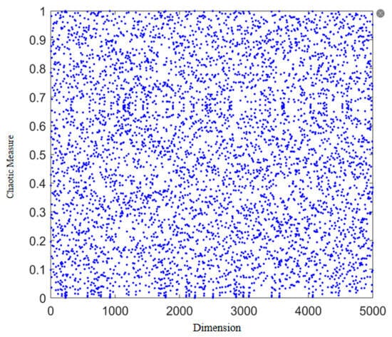
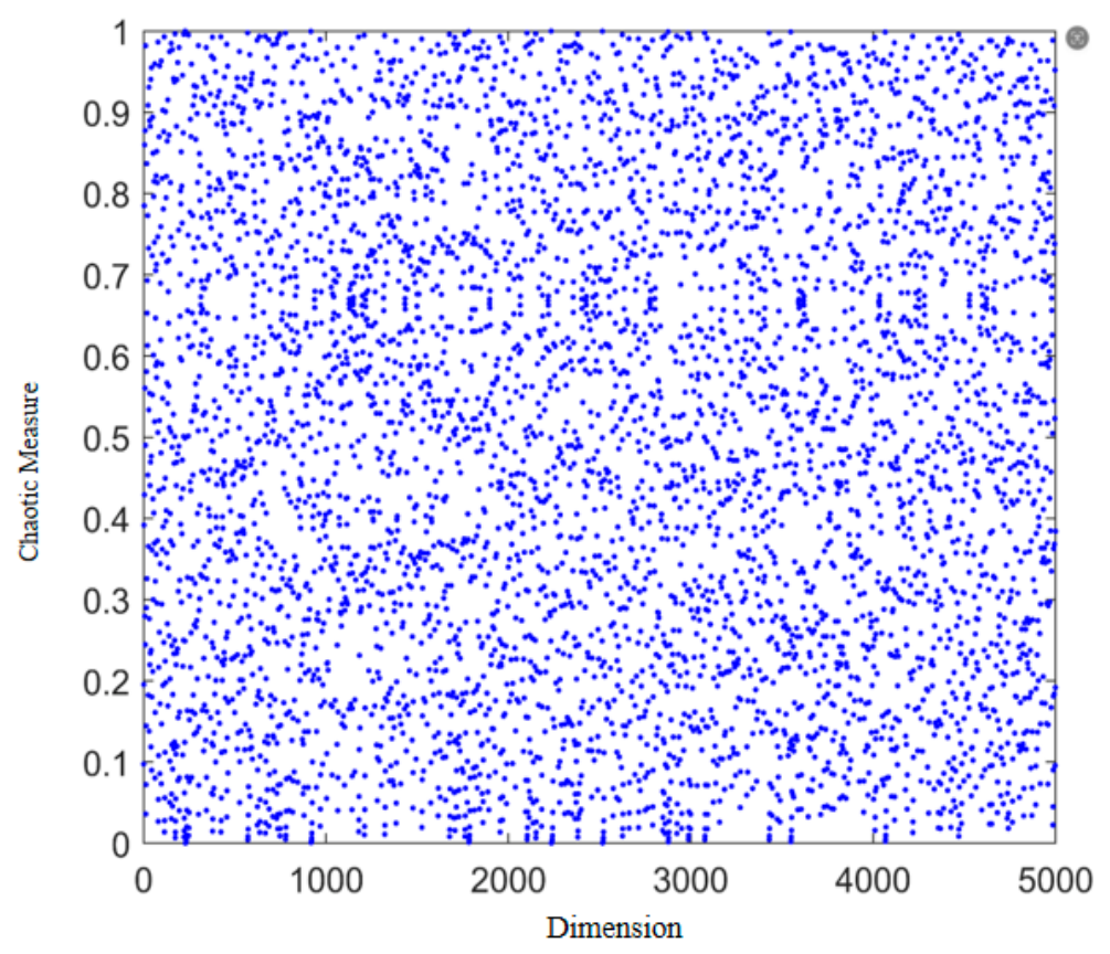
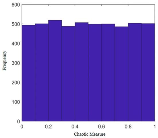
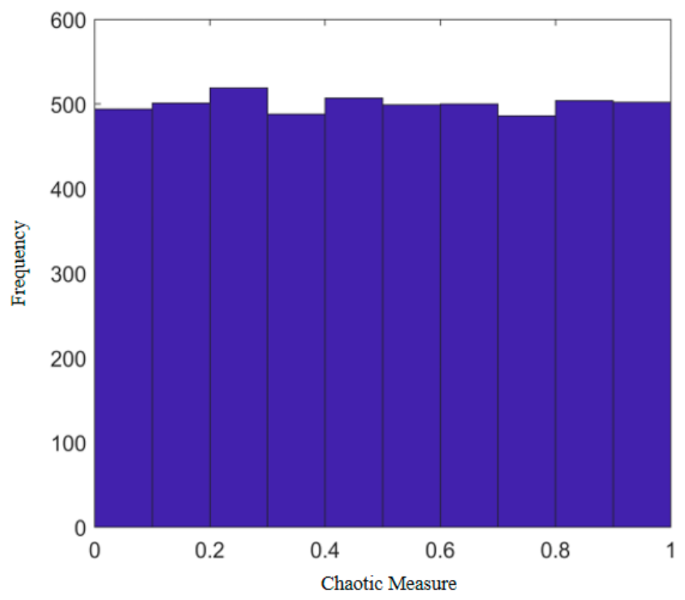
The distribution of the chaotic mapping sequence presented in this paper is shown in Figure 4, with $\lambda =0.4$. Observation of Figure 5 reveals that the sequence generated by the mapping exhibits uniform distribution, with the distribution density being nearly consistent across all mapped values.

Figure 4. Distribution of chaotic sequences.

Figure 5. Statistical distribution of chaotic sequences.

During the initialisation phase of the GWO algorithm, new population positions generated within the solution space via chaotic mapping are employed. This addresses the issue of random distribution within the initial population of the GWO algorithm, thereby enhancing its convergence speed.

(2)

Refining the Convergence Parameter Update Strategy

In Equation (17), the convergence factor $A$ varies with the convergence parameter $\alpha$. When $\left|A\right|>1$, the wolf pack searches for prey throughout the entire hunting area; When $\left|A\right|<1$, the wolf pack continuously encircles the optimal prey. The variation formula for the convergence parameter $\alpha$ is

$$a=2\left(1-{\displaystyle \frac{t}{t_{\max }}}\right)$$

(17)

where $t_{\max }$ denotes the maximum iteration count.

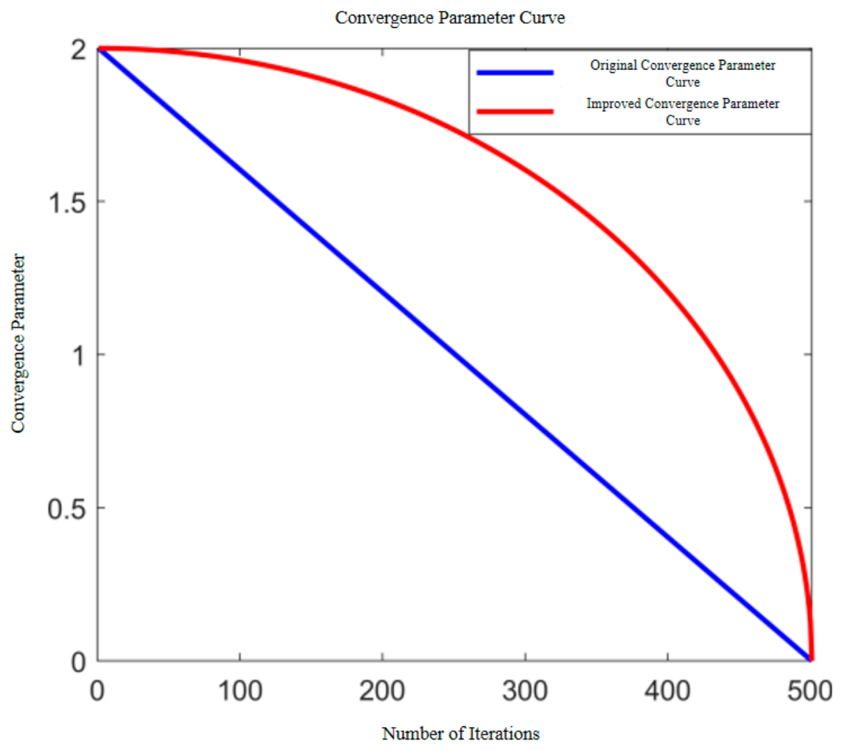
In Equation (17), the convergence parameter $\alpha$ exhibits linear decay. Different update strategies for convergence parameter $\alpha$ significantly influence the GWO algorithm’s global search capability and local exploitation capability. The optimisation process of GWO exhibits non-linear characteristics. Employing a linear update mechanism fails to fully realise its potential for global exploration and local refinement, potentially leading to entrapment in local optima. To balance the algorithm’s performance in global search and local precision, this paper proposes a convergence parameter update strategy based on the variation pattern of a quadrantal ellipse, as shown in Equation (18):

$$a=2\cdot \sqrt{1-{\displaystyle \frac{t^2}{t_{{\max }^2}}}}$$

(18)

As illustrated in Figure 6, compared to the pre-improved convergence parameter update mechanism, the convergence parameter decreases at a slower rate during the initial stages of iteration, thereby enhancing the algorithm’s global search capability. Conversely, in the later stages of iteration, the convergence parameter decreases at an accelerated rate, improving the algorithm’s precision in localised searches.

Figure 6. Convergence parameter curve.

(3)

Improved adaptive position update strategy

In Equation (13), the updated position of each grey wolf individual is derived by assigning equal weights to the positions of the $\alpha ,\beta ,\delta$ wolves [15]. However, the differing characteristics and decision-making capabilities of the $\alpha ,\beta ,\delta$ wolves result in the original grey wolf algorithm converging at a relatively slow rate. Furthermore, within the GWO, once the $\alpha ,\beta ,\delta$ are initialised, they are only updated during iterations when solutions with superior fitness values emerge. When $\alpha ,\beta ,\delta$ become trapped in local optima, the entire population cannot attain the global optimum solution.

This paper proposes an adaptive dynamic weight position update strategy combining adaptive and fitness-based approaches, formulated as follows:

$$W_1={\displaystyle \frac{\left|X_1\right|}{\left|X_1+X_2+X_3\right|}}$$

(19)

$$W_2={\displaystyle \frac{\left|X_2\right|}{\left|X_1+X_2+X_3\right|}}$$

(20)

$$W_3={\displaystyle \frac{\left|X_3\right|}{\left|X_1+X_2+X_3\right|}}$$

(21)

$${\omega }_{\alpha }={\displaystyle \frac{f_{\alpha }}{f_{\alpha }+f_{\beta }+f_{\delta }}}$$

(22)

$${\omega }_{\beta }={\displaystyle \frac{f_{\beta }}{f_{\alpha }+f_{\beta }+f_{\delta }}}$$

(23)

$${\omega }_{\delta }={\displaystyle \frac{f_{\delta }}{f_{\alpha }+f_{\beta }+f_{\delta }}}$$

(24)

$$X(t+1)=\left({\displaystyle \frac{2t}{t_{\max }}}+1\right)\cdot {\displaystyle \frac{{\omega }_{\alpha }{W}_1{X}_1+{\omega }_{\beta }{W}_2{X}_2+{\omega }_{\delta }{W}_3{X}_3}{3}}$$

(25)

Here, $W_1,W_2,W_3$ denotes the positional weight from ω wolf to $\alpha ,\beta ,\delta$ wolf, while $f_{\alpha },f_{\beta },f_{\delta }$ represent the fitness value of $\alpha ,\beta ,\delta$ wolf. The position update for each grey wolf individual per iteration is given by Equation (25). By integrating the adaptive stepping strategy of grey wolf individuals with fitness weighting, the weighting applied by $\alpha ,\beta ,\delta$ wolf to position updates dynamically adjusts. This reflects the influence of different leadership strata within the grey wolf population on individual wolves, thereby enhancing the global search capability and local search precision of the grey wolf optimisation algorithm [16]. In summary, compared with the standard GWO, the three proposed modifications jointly improve population diversity, the balance between global exploration and local exploitation, and convergence accuracy. Their effectiveness is validated in Section 4, where the IGWO outperforms GWO, PSO, and TLBO on the benchmark functions in terms of both average convergence accuracy and robustness.

3.3. LSTM Neural Networks

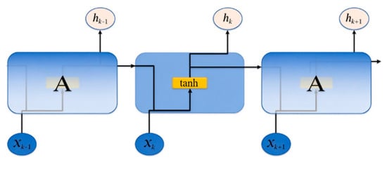
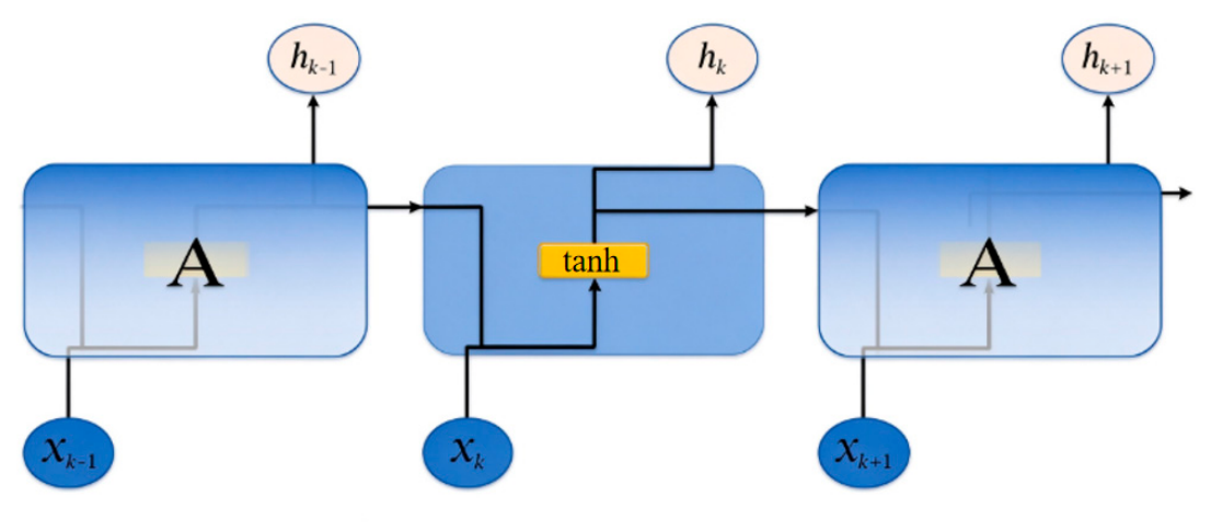
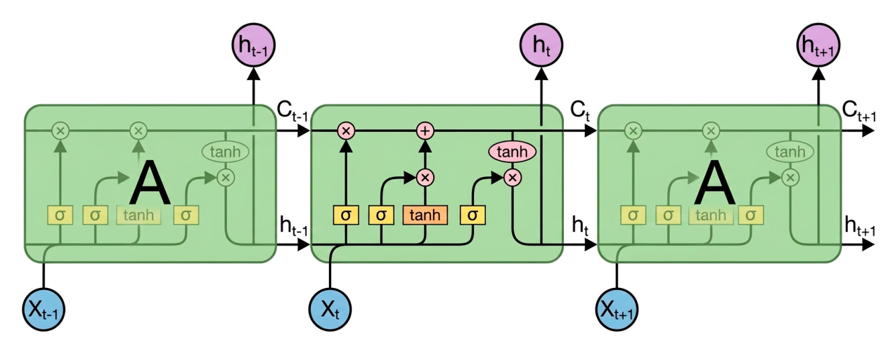
Long Short-Term Memory (LSTM) neural networks were proposed to address the long-term dependency issues inherent in Recurrent Neural Networks (RNNs). They are capable of learning long-term dependency information, thereby mitigating the problems of vanishing gradients and exploding gradients to a certain extent [17,18]. Structural comparisons between RNN and LSTM neural networks are illustrated in Figure 7 and Figure 8.

Figure 7. RNN architecture.

Figure 8. LSTM architecture.

LSTM introduces a gate mechanism upon the foundation of RNN, incorporating a forget gate, an input gate, and an output gate to regulate the flow and loss of features.

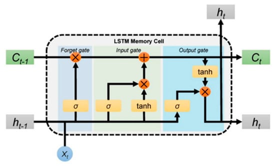
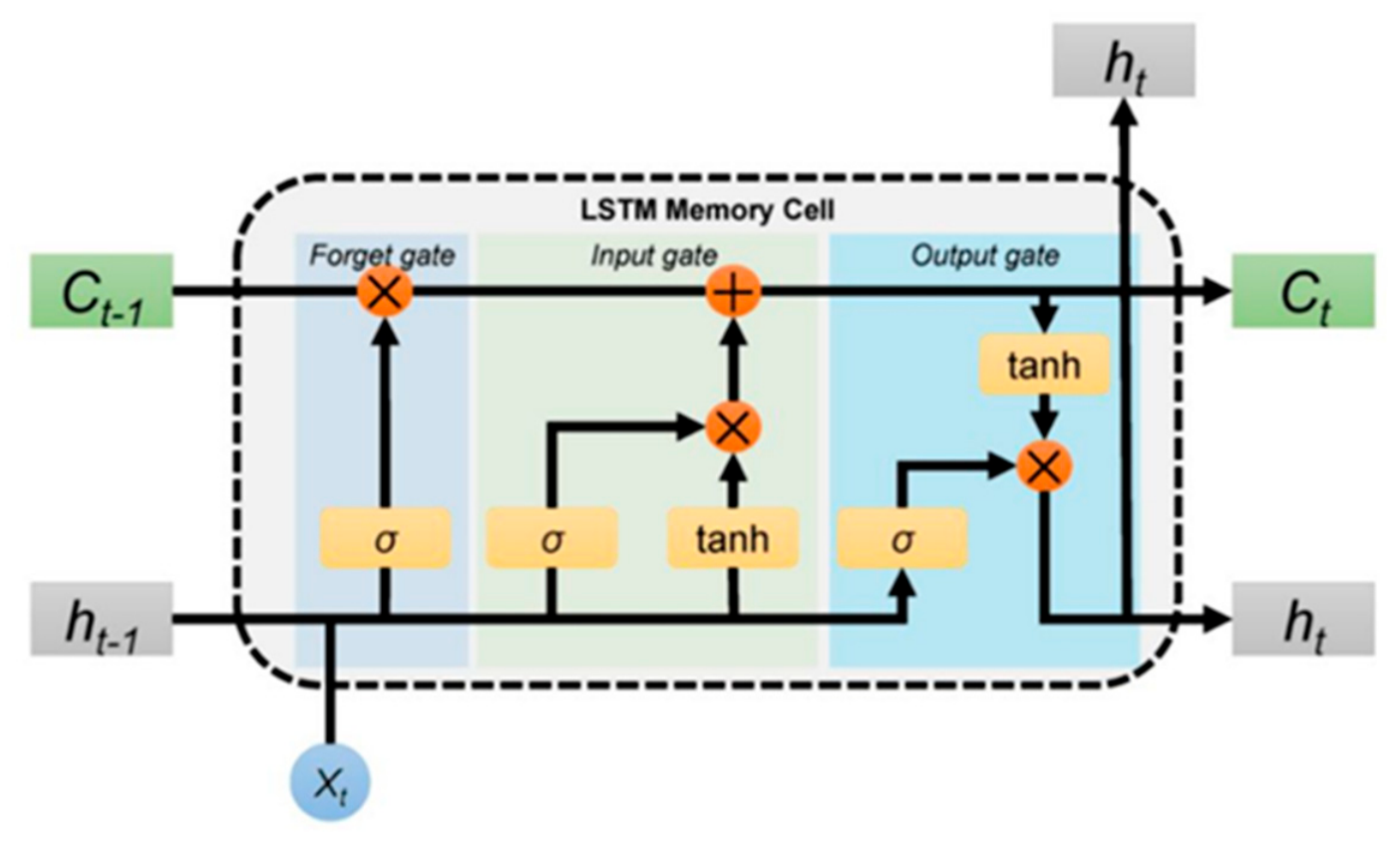
The state variables within the LSTM recurrent structure can be categorised as the cell state and the hidden state $h_t$. $c_t$ preserves long-term state information, whilst $h_t$ is responsible for transmitting short-term state information. The internal structure and mathematical representation of an LSTM neuron are shown in Figure 9 below:

Figure 9. Internal structure of an LSTM node.

(1)

The Gate of Oblivion

The function of the forget gate is to filter information, selecting characteristic data from the previous cell state $c_{t-1}$ to compute the current cell state $c_t$. Its output value ranges between 0 and 1; the closer it is to 0, the more historical information should be discarded, and the closer it is to 1, the opposite applies. The mathematical expression for the forget gate is as follows:

$$f_t=\sigma \left(W_f\cdot \left[h_{t-1},x_t\right]+b_f\right)$$

(26)

In the equation, $f_t$ denotes the output of the forgetting gate at time $t$, $\sigma \left(f\right)$ is the sigmoid function, $W_i$ denotes the weight of the forgetting gate, $b_f$ denotes the bias vector for the hidden layer, $h_{t-1}$ denotes the hidden state output of the state unit at the previous time step, $x\left(t\right)$ denotes the input at time $t$.

(2)

Input gate

The input gate determines which information from input $x\left(t\right)$ is retained in cell state $c_t$. It comprises two components: firstly, the sigmoid layer determines the updated value; secondly, the tanh layer generates a new candidate value vector. Its mathematical expression is as follows:

$$i_t=\sigma \left(W_i\left[h_{t-1},x_t\right]+b_i\right)$$

(27)

$$C_{tt}=\tanh \left(W_c\left[h_{t-1},x_t\right]+b_c\right)$$

(28)

In the equation, $i_t$ and $x_t$ denote the input gate outputs at time $t$, $W_i$ represents the input layer weights, $b_i$ denotes the input layer bias, $C_{tt}$ signifies the candidate cell state, and $W_c$ denotes the candidate cell state weights, $b_c$ denotes the cellular candidate state bias, $\tanh (\hspace{0.33em})$ denotes the hyperbolic tangent activation function.

The cellular state $C_t$ at time $t$ can be expressed as

$$C_t=f_t\odot C_{t-1}+i_t\odot C_{tt}$$

(29)

where $\odot$ denotes the vector-scalar product.

(3)

Output Gate

The output gate determines the output of the state unit at time $t$, with its mathematical expression as follows:

$$O_t=\sigma \left(W_o\left[h_{t-1},x_t\right]+b_o\right)$$

(30)

In the equation, $O_t$ denotes the output of the output gate, $W_o$ represents the output layer weights, and $b_o$ signifies the output layer bias.

When employing LSTMs for forecasting, multiple hyperparameters significantly influence model performance, including initial weights and biases, as well as the number of hidden layer neurons [19].

Although conventional LSTM networks can model long-term dependencies in time-series data, their network architecture and hyperparameters are commonly determined through manual experience. Parameters such as the learning rate, number of hidden units, batch size, and time-step length can substantially affect convergence and classification performance. When the training data contain noise, the inter-class differences are small, or the operating conditions vary, a conventional LSTM may suffer from slow convergence, local optima, overfitting, or imbalanced recognition ability among different fault classes. In addition, a conventional LSTM generally uses fixed network parameters and therefore has limited adaptability to different datasets and operating conditions.

To optimise both the accuracy and efficiency of the predictive model while addressing the issue of random hyperparameter selection in LSTM neural networks, this study employs an enhanced grey wolf optimisation algorithm for iterative hyperparameter tuning of the forecasting model. To automate the selection of the LSTM hyperparameters, the IGWO algorithm is employed to optimize the key parameters of the LSTM network. The optimized parameters and their search ranges are as follows: the learning rate ∈ [10⁻⁴~10⁻²], the number of hidden neurons ∈ [8~128], the batch size ∈ [16~128], and the time-step length ∈ [4~64]. The objective (fitness) function of the IGWO is defined as the classification error on the validation set, where Acc_val denotes the accuracy of the LSTM model on the validation set. The IGWO iteratively minimizes F to search for the optimal hyperparameter combination. The optimal parameters are then used to retrain the final LSTM model on the training set, and its generalization performance is evaluated on the isolated test set.

3.4. Vibration Signal Feature Extraction

This section employs the previously mentioned CEEMDAN algorithm to perform decomposition and feature extraction on vibration signals, essentially constructing and solving a constrained variational problem. Specifically, by identifying multiple modal functions, the objective is to minimise the total sum of spectral estimation bandwidths for the decomposed signal modes, whilst satisfying the constraint that the sum of all modes equals the original input signal. This algorithm is particularly well-suited for decomposing measurement signals containing several dominant internal modes, a characteristic commonly found in noisy vibration signals. Furthermore, various time-frequency domain feature parameters, as shown in Table 1 and Table 2, are extracted from the decomposed vibration signals.

Table 1. Formulas for Time-domain feature parameters.

Time-Domain Features	Formula Calculation	Time-Domain Features	Formula Calculation
mean value	$\overline{x}={\displaystyle \frac{1}{N}}{\displaystyle \sum _{i=1}^N{x}_i}$	Peak-to-peak	$x_{peak}=x_{\max }-x_{\min }$
variance	${\delta }^2={\displaystyle \frac{1}{N}}{\displaystyle \sum _{i=1}^N{\left(x_i-\overline{x}\right)}^2}$	root mean square	$RMS=\sqrt{{\displaystyle \frac{{\displaystyle \sum _{i=1}^N{x}_i^2}}{N}}}$
root amplitude	$x_r={\left({\displaystyle \frac{1}{N}}{\displaystyle \sum _{i=1}^N\sqrt{\left|x_i\right|}}\right)}^2$	Skewness	$Skew={\displaystyle \frac{{\displaystyle \sum _{i=1}^N{\left(x_i-\overline{x}\right)}^3}}{N{\delta }^3}}$
steepness	$\beta ={\displaystyle \frac{{\displaystyle \sum _{i=1}^N{\left(x_i-\overline{x}\right)}^4}}{N{\delta }^4}}$	wave factor	$S_f={\displaystyle \frac{RMS}{\left|\overline{x}\right|}}$
Peak factor	$I_p={\displaystyle \frac{x_{peak}}{RMS}}$	Pulse factor	$C_f={\displaystyle \frac{x_{peak}}{\left|\overline{x}\right|}}$
Safety factor	$C_e={\displaystyle \frac{x_{peak}}{x_r}}$

Table 2. Frequency domain characteristic parameter formulas.

Frequency Domain Features	Formula Calculation
root mean square frequency	$MSF={\displaystyle \frac{{\displaystyle \sum _{i=0}^n{f}_i^{2}P\left(f_i\right)}}{{\displaystyle \sum _{i=0}^{n}P\left(f_i\right)}}}$
root mean square frequency	$RMSF=\sqrt{MSF}$
Centre of gravity frequency	$FC={\displaystyle \frac{{\displaystyle \sum _{i=0}^n{f}_{i}P\left(f_i\right)}}{{\displaystyle \sum _{i=0}^{n}P\left(f_i\right)}}}$
Frequency variance	$VF={\displaystyle \frac{{\displaystyle \sum _{i=0}^n{\left(f_i-FC\right)}^{2}P\left(f_i\right)}}{{\displaystyle \sum _{i=0}^{n}P\left(f_i\right)}}}$
Frequency standard deviation	$RVF=\sqrt{VF}$

4. Improved Grey Wolf Algorithm Test

To evaluate the improved grey wolf optimisation algorithm’s computational capabilities, six test functions were selected for simulation testing. Concurrently, the improved grey wolf optimisation algorithm (IGWO) was compared against the standard grey wolf optimisation algorithm (GWO), particle swarm optimisation (PSO), and the basic teaching–learning optimisation algorithm (TLBO). The mathematical expressions of the test functions are presented in Table 3.

Table 3. Benchmark function table (Dimension = 30, Solution = 0).

Function	Function Expression	Scope
F1	$f_1(x)={\displaystyle \sum _{i=1}^n}{X}_i^2$	[−100, 100]
F2	$f_2\left(x\right)={\displaystyle \sum _{i=1}^n}\left|X_i\right|+{\displaystyle \prod _{i=1}^n}\left|X_i\right|$	[−10, 10]
F3	$f_3\left(x\right)={\mathrm{m}\mathrm{a}\mathrm{x}}_i\{\left|x_i\right|,1\le i\le n\}$	[−100, 100]
F4	$f_4\left(x\right)={\displaystyle \sum _{i=1}^{n-1}}[100{(x_i+1-x_i^2)}^2+{(x_i-1)}^2]$	[−30, 30]
F5	$f_5\left(x\right)={\displaystyle \sum _{i=1}^n}{\left(\left|x_i+0.5\right|\right)}^2$	[−100, 100]
F6	$f_6\left(x\right)={\displaystyle \sum _{i=1}^n}\left[x_i^2-10\cos \left(2\pi x_i\right)+10\right]$	[−5.12, 5.12]

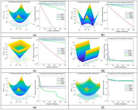
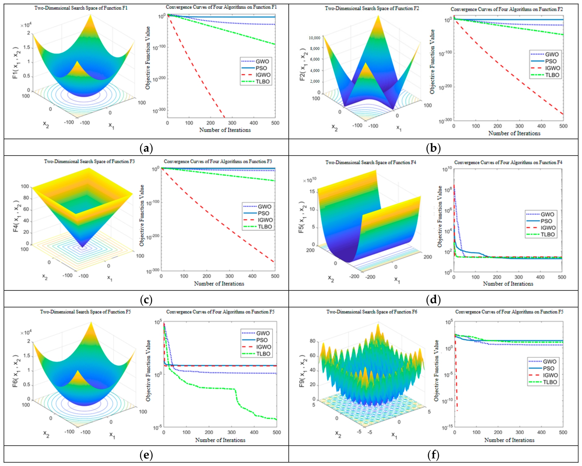
In the simulation experiments, the population size was set to 30, with a maximum iteration limit of 500. Each algorithm was independently run 20 times to obtain the most representative results. The convergence performance of various algorithms on the test function is illustrated in Figure 10.

Figure 10. Test function graph and convergence curves for each algorithm: (a) F1 function convergence curve; (b) F2 function convergence curve; (c) F3 function convergence curve; (d) F4 function convergence curve; (e) F5 function convergence curve; (f) F6 function convergence curve.

The test results demonstrate that for test functions F1, F2, F3, and F6, IGWO converged to optimal accuracy within the fewest iterations, outperforming other algorithms. For function F4, IGWO exhibited the fastest convergence rate, though its convergence accuracy was marginally inferior to PSO. Regarding test function F5, TLBO achieved the highest convergence accuracy, while IGWO’s performance on this function was merely adequate.

The results of the four algorithms on the test functions are shown in Table 4. The bolded data in the table represent the optimal results achieved by each algorithm during the optimisation process for each test function.

Table 4. Test results.

Test Function		GWO	PSO	TLBO	IGWO
F1	mean value	1.06 × 10−27	8.03 × 10−4	1.56 × 10−90	0
	standard deviation	1.09 × 10−27	7.68 × 10−4	1.47 × 10−90	0
F2	mean value	6.98 × 10−17	7.54 × 10−1	9.38 × 10−46	1.05 × 10−282
	standard deviation	3.21 × 10−17	3.67 × 10−1	6.75 × 10−46	0
F3	mean value	1.12 × 10−6	3.36 × 10−1	2.42 × 10−37	1.06 × 10−276
	standard deviation	1.44 × 10−6	1.03 × 10−1	1.77 × 10−37	0
F4	mean value	2.77 × 10	2.24 × 10	2.49 × 10	2.87 × 10
	standard deviation	9.33 × 10−1	1.08 × 10	4.16 × 10−1	1.05 × 10−2
F5	mean value	7.36 × 10−1	7.42 × 10−4	1.02 × 10−5	6.20
	standard deviation	4.30 × 10−1	8.04 × 10−4	1.03 × 10−5	4.6 × 10−1
F6	mean value	4.16	2.40 × 10	1.38 × 10	0
	standard deviation	2.46	6.46	7.09	0

Through the visual analysis presented in Table 4, it is evident that the three improvement measures introduced in this paper significantly enhance the performance of the grey wolf optimisation (GWO) algorithm. The improved grey wolf optimisation (IGWO) algorithm surpasses other algorithms in terms of average convergence accuracy during simulation testing, demonstrating superior global optimisation capabilities. Furthermore, observing the standard deviation of results across various test functions reveals that IGWO exhibits high robustness. Consequently, the improved Grey Wolf algorithm proposed herein possesses certain advantages.

5. Experimental Validation Analysis

5.1. Introduction to the Experimental Platform

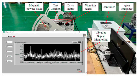
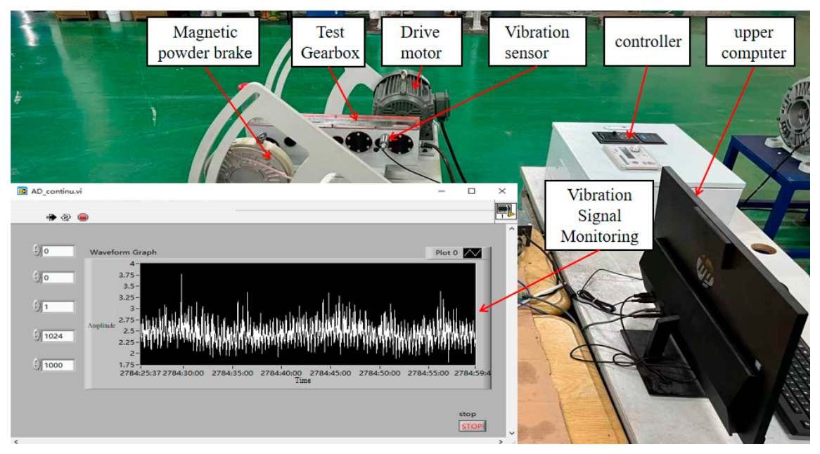
This study was conducted using an in-house laboratory-built gear transmission system online monitoring test bench, as illustrated in Figure 11. The test bench primarily comprises a magnetic powder brake connected via a coupling to the gearbox under test. This brake provides simulated load to the gearbox, with torque adjustable to deliver varying load levels. The gearbox under test receives power from a drive motor. A triaxial vibration sensor is mounted radially to the gear motion path, enabling real-time acquisition of vibration signals generated during gearbox operation. Data collected by the vibration sensor is displayed in real time on the host computer via a microcontroller, providing an intuitive visualisation of gearbox vibration signal variations. Furthermore, a full-lifecycle vibration monitoring experiment is conducted on the test bench. According to the temporal evolution of the vibration signals and the corresponding equipment condition, the entire operating process is divided into four stages: the healthy stage, the minor-wear stage, the severe-wear stage, and the failure stage. The healthy stage refers to the period during which the vibration characteristics remain within the baseline range established under normal operating conditions, without persistent fault-related deviations. The minor-wear stage refers to the period during which the vibration features exhibit a persistent deviation from the healthy baseline, indicating the initial development of a gear fault, while the gearbox can still operate normally without reaching the severe-wear condition. The severe-wear stage refers to the subsequent period in which the fault-related vibration characteristics become more pronounced and the gearbox exhibits significant wear, yet remains capable of operation under degraded conditions. The failure stage refers to the final period in which the gearbox reaches the predefined fault state or severe fault condition, with its vibration characteristics being markedly distinct from those of the healthy baseline. This stage-based division provides the basis for distinguishing conventional fault-state classification from early-fault warning. Upon completion, the generated vibration data is exported. Subsequently, employing the aforementioned methodology, the raw vibration signals undergo noise reduction and optimisation. Key time-frequency domain feature parameters are then extracted from these signals. These extracted parameters serve as input to an optimised LSTM neural network model, enabling analysis of the model’s diagnostic efficacy. The simulated operating conditions were a constant load, a rotational speed of 1400 r/min, and a vibration sensor sampling frequency of 2000 Hz. It should be noted that the experiments in this study were conducted on a gear transmission test rig constructed in a laboratory, rather than on an actual mining excavator. The test rig was designed to replicate the key dynamic characteristics of the gear transmission system in large mining excavators. Specifically, the gearbox is loaded via a magnetic powder brake with adjustable torque, thereby simulating the load conditions encountered in mining operations; a triaxial accelerometer mounted radially on the gearbox housing captures vibration signals, which are predominantly driven by gear meshing and contaminated by background noise, bearing a strong resemblance to the on-site signals from mining transmission systems. Furthermore, representative fault conditions (such as gear wear and failure) can be introduced and monitored under controlled, repeatable conditions, thereby enabling a quantitative evaluation of the proposed diagnostic methods.

Figure 11. Online monitoring test bench for gear transmission systems.

For each operating condition or fault category, the acquired vibration signals were segmented into 1000 samples, and the length of each sample was set to 1024 data points. Each sample was treated as an independent input instance for the subsequent feature extraction and fault diagnosis procedures. Before model training, the samples in each dataset were divided into training, validation, and test sets at a ratio of 70%, 15%, and 15%, respectively. Therefore, for each dataset containing 1000 samples, 700 samples were used for training, 150 samples were used for validation, and the remaining 150 samples were used for testing, as shown in Table 5 below. The data partitioning was performed before model training using a fixed random seed to ensure reproducibility. The training set was used to estimate the model parameters, whereas the validation set was used for hyperparameter selection, model comparison, and early-stopping decisions. The test set was completely isolated from the training and validation procedures and was used only for the final evaluation of the diagnostic performance.

Table 5. Fault Types and Sample Classification.

Fault Type	Training Set	Validation Set	Test Set	Dataset
Normal	700	150	150	Dataset 1
Minor wear	700	150	150	Dataset 2
Severe wear	700	150	150	Dataset 3
Failure	700	150	150	Dataset 4

5.2. Vibration Signal Denoising

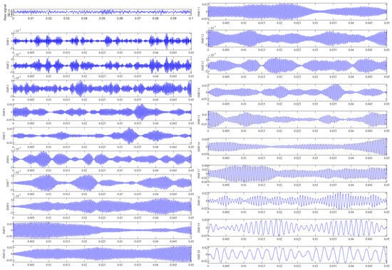
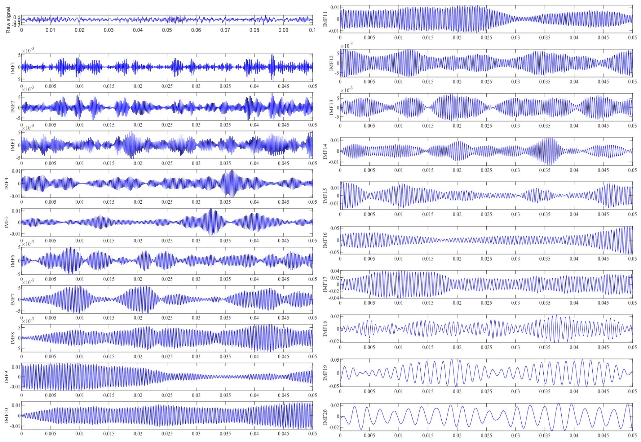
Employing the method proposed herein, the original signal was decomposed using the CEEMDAN approach, with the decomposition results illustrated in Figure 12.

Figure 12. CEEMDAN decomposition results.

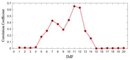
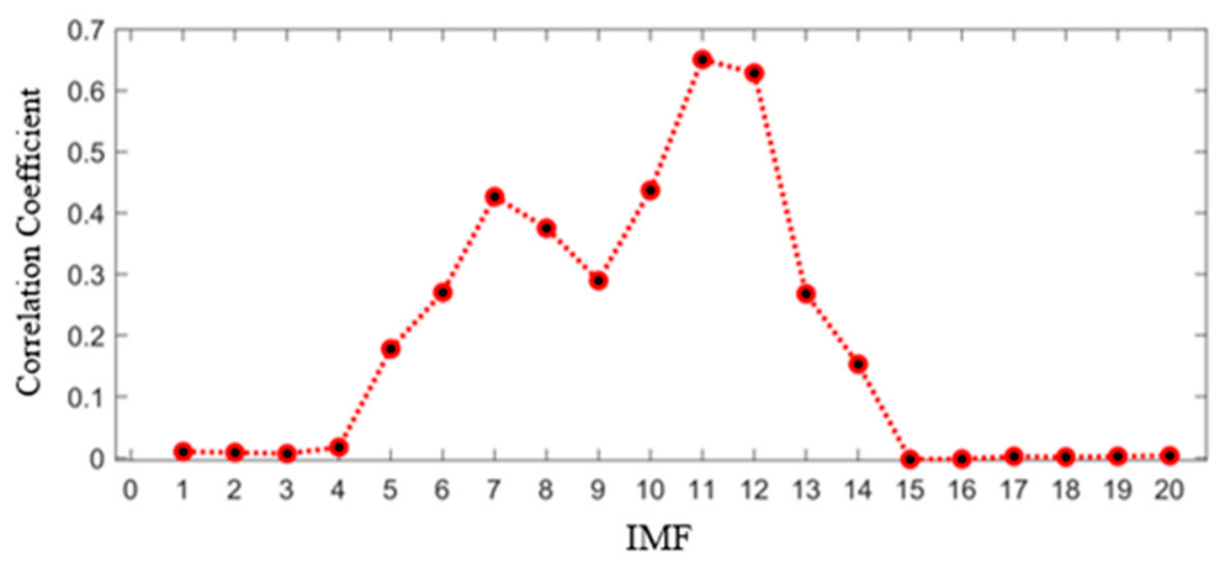
Upon completion of the decomposition, the Pearson correlation coefficients between each IMF and the original signal were calculated, with the results shown in Figure 13.

Figure 13. Correlation coefficients between each IMF and the original signal.

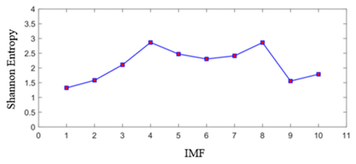
As shown in Figure 13, the correlation coefficients between IMF1 to IMF4 and IMF15 to IMF20 and the original signal are both below 0.1. Generally, CEEMDAN decomposes signals progressively from high to low frequencies. Consequently, IMF1 to IMF4 contain substantial high-frequency noise, while IMF15 to IMF20 predominantly comprise low-frequency components unrelated to transmission system vibrations. In accordance with the algorithmic specifications, IMFs with correlation coefficients below 0.1 were directly discarded. The remaining IMFs were then filtered using Shannon entropy, with the calculation segmented into 10 intervals. The average Shannon entropy for each IMF was computed, with the results presented in Figure 14.

Figure 14. Shannon Entropy of Each IMF in the New Assembly.

Comparing Figure 13 and Figure 14 reveals that for vibration signals within transmission systems, noise constitutes the primary component throughout the entire signal segment. Utilising the correlation coefficient criterion can only eliminate a portion of the smaller-amplitude high-frequency noise components and the low-frequency irrelevant components. At this stage, the background noise—which comprises numerous components—exhibits the highest correlation with the original signal. Consequently, it becomes impossible to effectively filter out the valid vibration components. Therefore, Shannon entropy must be employed to quantify the information content within the IMF.

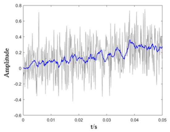
Based on Shannon entropy calculations, the four IMF components with the lowest entropy rankings in the new set (namely IMF5, IMF6, IMF13, and IMF14 from the original IMF set) were selected for reconstruction. The reconstructed signal is compared with the original signal as shown in Figure 15.

Figure 15. Comparison of reconstructed enhanced signal and original signal.

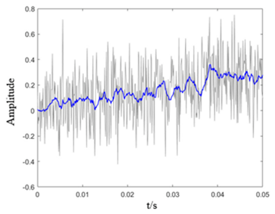
As can be seen from Figure 15, the reconstructed vibration signal following decomposition exhibits significantly reduced background noise compared to the original signal. The components characterising the transmission system’s vibration information are largely preserved, with the signal amplitude being distinctly pronounced.

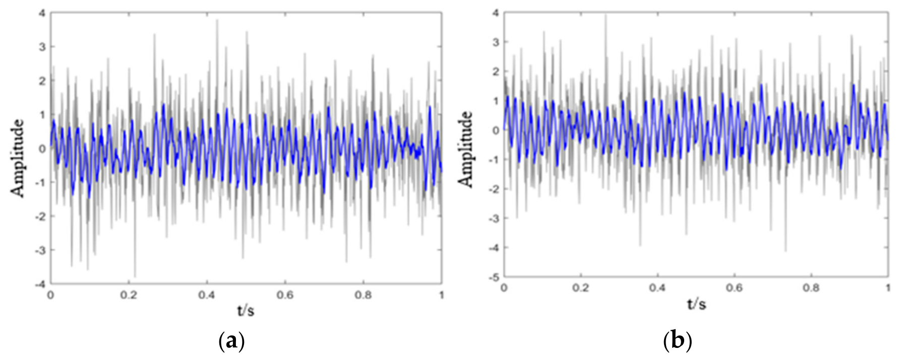
Furthermore, the results obtained using a moving average filter as a noise reduction method alongside the Least Mean Squares (LMS) algorithm are compared with the approach presented herein. The noise reduction outcomes are illustrated in Figure 16. The fundamental principle of the moving average filter involves comparing each data point within the signal with the average of several preceding and subsequent data points, subsequently replacing that data point with this average value. This effectively smooths the signal and reduces the impact of noise. The LMS algorithm is an adaptive filter that iteratively adjusts filter coefficients to minimise the mean square error of the signal. This approach is well-suited for scenarios where noise characteristics are unknown or variable, as the filter automatically adapts to changes in the input signal.

Figure 16. Results of different noise reduction methods: (a) Moving average filter noise reduction. (b) Least Mean Squares (LMS) algorithm noise reduction.

As can be seen from the figure, although the moving average filter denoising method and the least mean square (LMS) algorithm denoising method can to some extent attenuate background noise signals while substantially preserving the original vibration signal, their overall denoising performance still falls short of the method proposed in this paper. This further demonstrates the superiority of the approach outlined herein.

To further verify the denoising performance, quantitative comparisons were performed using SNR improvement, RMSE, correlation coefficient, spectral energy retention, kurtosis deviation, and entropy deviation. As shown in Table 6, the proposed CEEMDAN-based method achieved the highest SNR of 16.38 dB and the largest SNR improvement of 10.58 dB. In comparison, the SNR improvements obtained by moving-average and LMS filtering were 4.92 dB and 6.66 dB, respectively.

Table 6. Quantitative comparison of different denoising methods.

Method	SNR/dB	SNR Improvement/dB	RMSE	Correlation Coefficient	Spectral Energy Retention/%	Kurtosis Deviation/%	Entropy Deviation/%
Noisy signal	5.80	—	0.184	0.742	112.60	31.80	18.40
Moving-average filtering	10.72	4.92	0.109	0.861	84.60	21.50	12.70
LMS filtering	12.46	6.66	0.086	0.903	91.80	13.20	8.60
CEEMDAN-based method	16.38	10.58	0.052	0.962	97.30	6.40	4.10

The CEEMDAN-based method also produced the lowest RMSE of 0.052 and the highest correlation coefficient of 0.962, indicating that the reconstructed signal was closer to the reference signal than the signals obtained using the other two filtering methods. In addition, the spectral energy retention of CEEMDAN was 97.30%, which was closer to the reference energy than those of moving-average filtering and LMS filtering. The kurtosis and entropy deviations were 6.40% and 4.10%, respectively, demonstrating that the proposed method better preserved the impulsive characteristics and information complexity of the vibration signal.

Overall, the numerical results are consistent with the waveform and spectral observations in Figure 16. The CEEMDAN-based method provides a better balance between noise suppression and preservation of fault-related signal characteristics.

5.3. Fault Identification Experiment

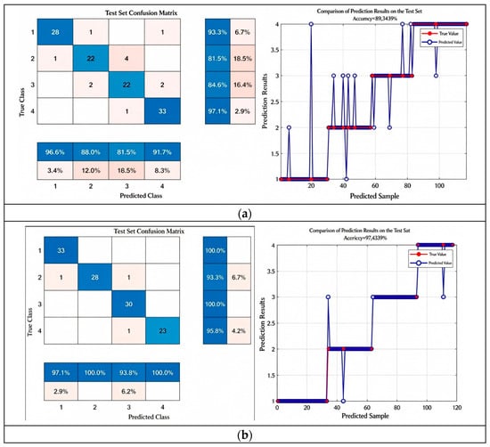
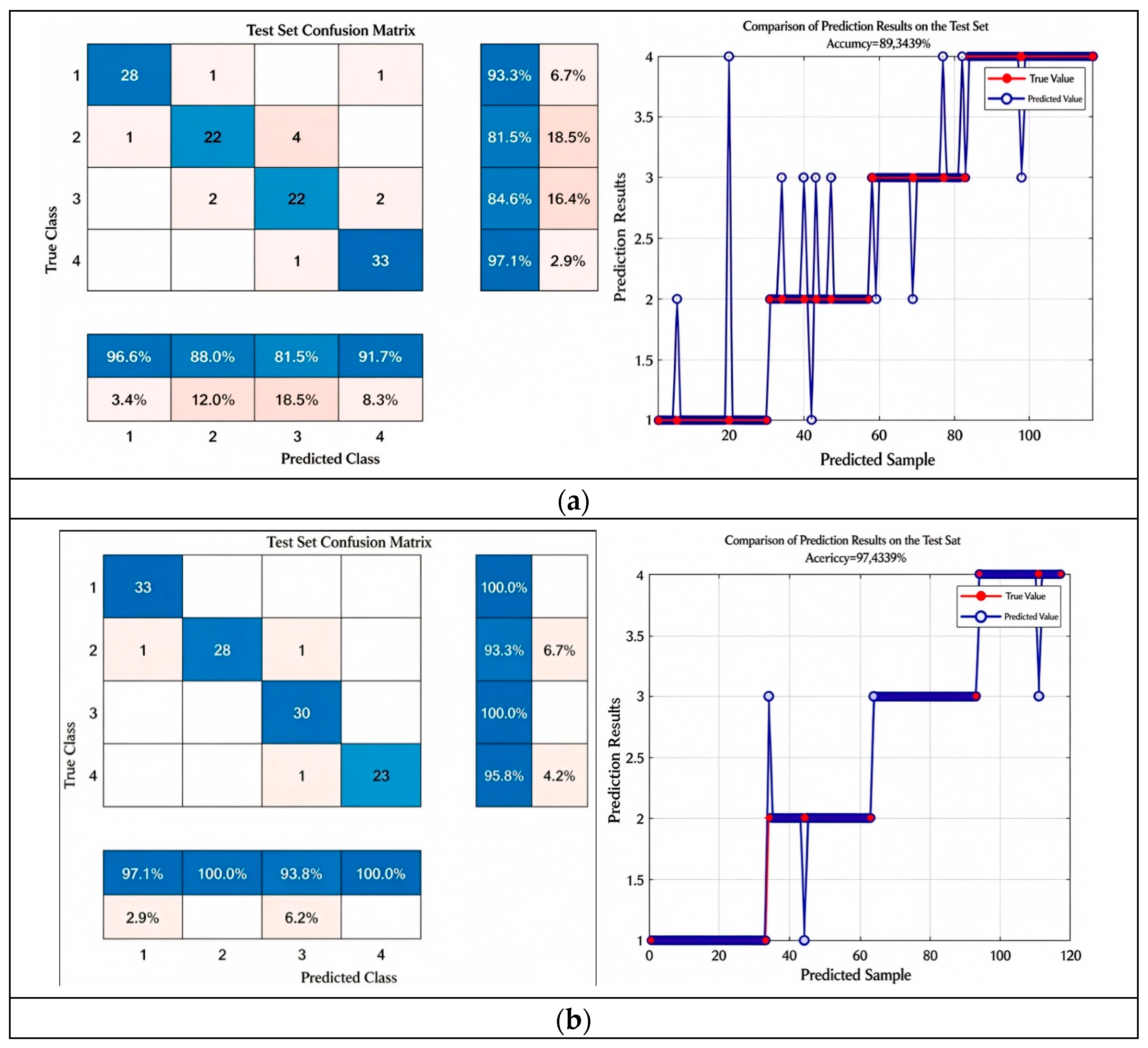
Following completion of the experiment, the vibration data collected during the process were divided into four datasets, and their classification recognition accuracy was verified, with results shown in Figure 17. Here, 1, 2, 3, and 4 represent normal, minor wear, severe wear, and failure, respectively. To evaluate the diagnostic performance of the optimised LSTM neural network fault model, this study conducted experimental comparisons of various models. The test set comprised 1000 samples, each with a length of 1024. The recognition accuracy of the test set under different methods is presented in Table 4, where 1D-LSTM denotes the model prior to improvement.

Figure 17. Fault detection accuracy rates across datasets: (a) Model accuracy before optimization. (b) Model accuracy before optimization.

Table 7 presents the class-wise diagnostic performance of the proposed model on the test set. The model achieved an F1-score above 94% for the Normal and Failure categories, indicating reliable recognition of normal operation and failure conditions. The F1-scores for Minor wear and tear and Severe wear and tear were 84.62% and 83.02%, respectively. These values are lower than those of the other two categories, mainly because the two wear-related conditions have more similar vibration characteristics and are therefore more difficult to distinguish.

Table 7. Diagnostic performance of the proposed model across different categories on the test set.

Category	Precision	Recall	F1-Score
Category 1: Normal	96.55%	93.33%	94.92%
Category 2: Minor wear and tear	88.00%	81.48%	84.62%
Category 3: Severe wear and tear	81.48%	84.62%	83.02%
Category 4: failure	91.67%	97.06%	94.29%

The macro-averaged results were 89.43% for precision, 89.12% for recall, and 89.21% for F1-score, while the balanced accuracy was 89.12%. The close values of Macro-F1 and balanced accuracy indicate that the model does not rely solely on the performance of a single dominant class. Instead, it provides relatively balanced recognition across all four categories. The confusion matrix further confirms that most samples were correctly classified, while the main misclassifications occurred between the two wear-related categories.

As shown in Table 8, when experimentally validated across four distinct datasets, the improved LSTM neural network model proposed in this chapter consistently achieves higher test accuracy than the original neural network model (1D-LSTM). Specifically, on Dataset 1, the improved LSTM model demonstrates a 10.17% accuracy improvement over the original convolutional neural network, while on Datasets 2, 3, and 4, accuracy improved by 5.26%, 6.99%, and 9.07%, respectively, with an average accuracy increase of approximately 7.87%, demonstrating the effectiveness of the enhancements. Furthermore, the improved LSTM model exhibited smaller variations in accuracy across different datasets compared to the original LSTM model, indicating that the enhancements strengthened the model’s stability and generalization capabilities.

Table 8. Average test accuracy of fault diagnosis across different datasets.

Method	Accuracy/%
	Dataset1	Dataset2	Dataset3	Dataset4
1D-LSTM	86.7	92.6	89.8	87.6
proposed method	96.87	97.86	96.79	96.67
Gap	10.17	5.26	6.99	9.07

To demonstrate the separate contributions of the CEEMDAN preprocessing and the IGWO, an ablation study was conducted by comparing four configurations: (1) raw signal + LSTM, (2) raw signal + IGWO-LSTM, (3) CEEMDAN + LSTM, and (4) CEEMDAN + IGWO-LSTM (the proposed method). Comparing configurations (1) and (2) isolates the contribution of the IGWO; comparing (1) and (3) isolates the contribution of the CEEMDAN preprocessing; and configuration (4) reveals their combined effect. All configurations used the same dataset, sample length, train/validation/test split, and evaluation protocol to ensure a fair comparison. The results are summarized in Table 9.

Table 9. Table of Ablation Experiments.

Ablation Settings	Pre-Treatment	Classifier	D1	D2	D3	D4	Average
(1) Raw + LSTM	None	LSTM	81.35	87.42	84.51	82.68	84.0
(2) Raw + IGWO-LSTM	None	IGWO-LSTM	85.10	90.35	87.68	85.87	87.25
(3) CEEMDAN + LSTM	CEEMDAN	LSTM	86.70	92.60	89.80	87.60	88.87
(4) CEEMDAN + IGWO-LSTM (This article)	CEEMDAN	IGWO-LSTM	96.87	97.86	96.79	96.67	96.74

From Table 9, comparing (1) with (3) shows that the CEEMDAN preprocessing alone improves the average diagnostic accuracy by approximately 4.87 percentage points (from 84.0% to 88.87%), demonstrating its contribution in enhancing fault-related features. Comparing (1) with (2) shows that the IGWO alone improves the average accuracy by approximately 3.25 percentage points (from 84.0% to 87.25%). The proposed method (4) achieves the highest average accuracy of 96.74%, indicating that the CEEMDAN preprocessing and the IGWO provide complementary benefits.

To further evaluate the fault diagnosis effectiveness of the proposed method, this chapter compares it with other approaches. The comparison methods include: Reference [20] combines oversampling techniques for sample features with SVM, employs KNN to handle noise, and uses SVM-trained data (denoted as SVM + KNN); Reference [21] employs the Hjorth parameter in the time domain for fault diagnosis. It calculates the original vibration signal using Empirical Mode Decomposition (EMD) and utilizes the Hjorth parameter to compute the feature vector (denoted as VMD + Hjorth). Reference [22] proposed a Deep Wavelet Autoencoder (DWAE) method based on Extreme Learning Machines (ELM), employing ELM for classification (denoted as DWAE + ELM). Reference [23] introduced a multi-label imitation learning framework utilizing Deep Reinforcement Learning (DRL) to mimic object features (denoted as DRL). Reference [24] combines Variational Mode Decomposition (VMD) with Deep Belief Networks (DBN) (denoted as VMD + DBN). To ensure a fair comparison, all competing methods were evaluated under the same experimental settings, with the results presented in Table 10. Specifically, they used the same dataset, the same sample length, and the same training/validation/test partition (70%/15%/15% with a fixed random seed) and the same test set as the proposed method; the evaluation metrics and protocol were also identical.

Table 10. Comparison of the Improved Model with Other Methods.

Method	SVM + KNN	VMD + Hjorth	DWAE + ELM	DRL	VMD + DBN	Proposed Method
Accuracy	93.25%	93.64%	95.33%	94.21%	94.53%	96.74%

5.4. Practical Applicability and Limitations

From a practical perspective, the proposed method has both advantages and limitations. Based on an indicative estimate for processing a vibration-signal segment containing approximately 4096 samples on a standard industrial computer or edge-computing platform, the complete online pipeline may take approximately 0.2–2.0 s per segment. CEEMDAN decomposition is expected to be the most time-consuming stage, requiring approximately 0.1–1.5 s, while feature extraction and LSTM inference may take approximately 0.01–0.1 s and less than 0.01 s, respectively. These values are approximate estimates rather than measured results and may vary depending on the processor, signal length, CEEMDAN ensemble size, number of retained intrinsic mode functions, and software implementation. The IGWO and LSTM training are performed offline and are therefore excluded from the online inference time.

The main advantage of the proposed method is that CEEMDAN preprocessing combined with the optimized LSTM classifier maintains relatively stable diagnostic performance under the operating conditions evaluated in this study and under moderate sensor noise. Its main limitation is the higher computational cost of CEEMDAN compared with simple filtering methods. Therefore, the current method is more suitable for deployment on an industrial computer, edge-computing platform, or remote monitoring server than on a highly resource-constrained embedded system.

Future work will focus on reducing the number of CEEMDAN ensemble realizations, limiting the number of retained intrinsic mode functions, and developing lightweight preprocessing and classification modules. These measures are expected to reduce inference time while maintaining acceptable diagnostic accuracy.

6. Conclusions

To address the issues of low intelligence and inadequate automation in the operation and maintenance of large-scale mining machinery, this paper proposes a fault diagnosis model based on an enhanced long short-term memory (LSTM) neural network optimised by the augmented grey wolf optimisation algorithm. First, vibration signals from the in-service transmission system are acquired via a gear transmission system online monitoring test rig. Subsequently, the raw vibration signals are subjected to denoising and decomposition using the complete ensemble empirical mode decomposition with adaptive noise (CEEMDAN) algorithm, and comparative analyses reveal that this algorithm exhibits significant advantages in denoising performance over the moving average filtering and least mean squares (LMS) algorithms. Key discriminative features are then extracted to serve as input parameters for the enhanced LSTM neural network model. The diagnostic performance of the model before and after enhancement is systematically analysed and verified, with experimental results demonstrating that the enhanced model achieves an average diagnostic accuracy of 96.74%. Compared with classical machine learning-based methods—namely the SVM + KNN and VMD + Hjorth combinations the proposed method improves diagnostic accuracy by 3.49% and 3.1%, respectively. It also outperforms the advanced machine learning methods of DWAE + ELM and DRL, yielding accuracy improvements of 1.41% and 2.53% in fault diagnosis. In comparison with the deep learning-based VMD + DBN method, the proposed method attains a further 2.21% increase in diagnostic accuracy.

References

- Wang, S.; Yumin, O.; Bang, D. Fault Diagnosis Technology for Mechanical Equipment and Its Development Trends. China High-Tech Enterp. 2015, 72–73. [Google Scholar] [CrossRef]
- Yu, W.; Zhao, C. Online Fault Diagnosis for Industrial Processes With Bayesian Network-Based Probabilistic Ensemble Learning Strategy. IEEE Trans. Autom. Sci. Eng. 2019, 16, 1922–1932. [Google Scholar] [CrossRef] [Scilit]
- Nong, H. Research on Fault Diagnosis Methods for Rolling Bearings in the Running Gear of Urban Rail Transit Trains. Master’s Thesis, Guangxi University, Nanning, China, 2022. [Google Scholar] [CrossRef]
- Zhang, Y.; Gao, X.; Ding, K.; Zhao, Y.; Lin, L. A Hybrid PCA and SOM Model for Bearing Fault Detection and Classification. In Proceedings of the 2021 Proceedings of the China Automation Conference; Chinese Association of Automation: Beijing, China, 2021; pp. 272–277. [Google Scholar] [CrossRef]
- Dadon, I.; Koren, N.; Klein, R.; Bortman, J. A realistic dynamic model for gear fault diagnosis. Eng. Fail. Anal. 2018, 84, 77–100. [Google Scholar] [CrossRef] [Scilit]
- Zhang, X.; Liu, Z.; Miao, Q.; Wang, L. An optimized time varying filtering based empirical mode decomposition method with grey wolf optimizer for machinery fault diagnosis. J. Sound Vib. 2018, 418, 55–78. [Google Scholar] [CrossRef] [Scilit]
- Qin, L.; Chen, Y.; Zhang, J.; Chen, H.; Shu, H. A Sensorless Gearbox Mechanical Pump and Electric Pump Condition Identification Algorithm. Control Inf. Technol. 2025, 119–126. [Google Scholar] [CrossRef]
- Lv, P. Research on Rolling Bearing Fault Diagnosis Methods Based on VMD and KELM. Master’s Thesis, North China University of Technology, Beijing, China, 2024. [Google Scholar] [CrossRef]
- Liu, R.; Yang, B.; Zio, E.; Chen, X. Artificial intelligence for fault diagnosis of rotating machinery: A review. Mech. Syst. Signal Process. 2018, 108, 33–47. [Google Scholar] [CrossRef] [Scilit]
- Zhang, S. Research on Device Identification and Anomaly Detection Algorithms in Industrial Control Systems. Master’s Thesis, Southeast University, Nanjing, China, 2023. [Google Scholar] [CrossRef]
- Luan, X.; Gao, X.; Xia, A.; Zhao, F.; Sha, Y.; Yang, J. A Rolling Bearing Fault Diagnosis Method Based on Gray Wolf Algorithm-Optimized Feature Modal Decomposition. J. Aeronaut. Eng. 2026, 41, 188–201. [Google Scholar] [CrossRef]
- Wang, Y. Research and Application of Infrasound-Based Leak Detection Methods for Heating Pipelines. Master’s Thesis, Qingdao University, Qingdao, China, 2023. [Google Scholar] [CrossRef]
- Cai, Y. Improvements to the Gray Wolf Optimization Algorithm and Its Application Research. Master’s Thesis, Jiangnan University, Wuxi, China, 2025. [Google Scholar] [CrossRef]
- Li, G.; Li, Z.; Wang, P.; Yang, R.; Jiang, C. Rolling Bearing Fault Diagnosis Strategy Based on IEGWO-VMD. J. Tianjin Univ. Technol. 2025, 41, 21–28. [Google Scholar] [CrossRef] [Scilit]
- Sherstinsky, A. Fundamentals of recurrent neural network (RNN) and long short-term memory (LSTM) network. Phys. D Nonlinear Phenom. 2020, 404, 132306. [Google Scholar] [CrossRef] [Scilit]
- Yu, J.; He, Y. Planetary gearbox fault diagnosis based on data-driven valued characteristic multigranulation model with incomplete diagnostic information. J. Sound Vib. 2018, 429, 63–77. [Google Scholar] [CrossRef] [Scilit]
- Zhong, J.; Feng, X.; Meng, X.; Fan, H.; Wang, Y.; Zhang, J. Deep Learning-Based Fault Diagnosis for Four-Column Hydraulic Presses. Mach. Tools Hydraul. 2026, 54, 200–206. [Google Scholar] [CrossRef]
- Lei, Y.; He, Z.; Lin, J.; Han, D.; Kong, D. Recent Advances in Fault Diagnosis Techniques for Planetary Gearboxes. J. Mech. Eng. 2011, 47, 59–67. [Google Scholar] [CrossRef] [Scilit]
- Wang, J.; Li, R.; Peng, X. Survey of nonlinear vibration of gear transmission systems. Appl. Mech. Rev. 2003, 56, 309–329. [Google Scholar] [CrossRef] [Scilit]
- Pan, L. Research on Deep Learning-Based Gearbox Fault Diagnosis Methods. Master’s Thesis, Yancheng Institute of Technology, Yancheng, China, 2023. [Google Scholar]
- Luo, X. Research on Rolling Bearing Fault Diagnosis Methods Based on Multi-Feature Fusion. Master’s Thesis, Xiangtan University, Xiangtan, China, 2021. [Google Scholar] [CrossRef]
- Shao, H.; Jiang, H.; Li, X.; Wu, S. Intelligent fault diagnosis of rolling bearing using deep wavelet auto-encoder with extreme learning machine. Knowl.-Based Syst. 2018, 140, 1–14. [Google Scholar] [CrossRef] [Scilit]
- Liao, Z.; Yan, H.; Tang, Z.; Chu, X.; Tao, T. Deep learning identifies leak in water pipeline system using transient frequency response. Process Saf. Environ. Prot. 2021, 155, 355–365. [Google Scholar] [CrossRef] [Scilit]
- Liu, R.; Mu, X.; Yang, J. Wind Power Prediction Based on Lasso-VMD-DBN. Shanxi Electr. Power 2024, 6, 1–5. [Google Scholar] [CrossRef] [Scilit]
Disclaimer/Publisher’s Note: The statements, opinions and data contained in all publications are solely those of the individual author(s) and contributor(s) and not of MDPI and/or the editor(s). MDPI and/or the editor(s) disclaim responsibility for any injury to people or property resulting from any ideas, methods, instructions or products referred to in the content. |
© 2026 by the authors. Licensee MDPI, Basel, Switzerland. This article is an open access article distributed under the terms and conditions of the Creative Commons Attribution (CC BY) license.