


Abstract
Precise lithofacies identification is essential for efficient deep shale gas exploration and predictive targeting of reservoir “sweet spots.” However, deep shale reservoirs exhibit strong heterogeneity. In addition, well-log signals are inherently susceptible to environmental noise, instrumental limitations, and acquisition anomalies, which further complicate facies classification and fine-scale characterization. Traditional facies recognition methods rely heavily on expert interpretation and qualitative assessment, resulting in low automation and limited quantitative accuracy. Moreover, because of the strong nonlinearity of well-log data and the complex coupling among geological features, existing machine learning models remain limited in deep feature extraction, adaptive representation, and generalization, making them insufficient for complex subsurface conditions. To address these challenges, this study proposes a novel intelligent facies identification framework, ZOA-PCNN-AT-SVM, which integrates the Zebra Optimization Algorithm (ZOA), Parallel Convolutional Neural Networks (PCNN), and a multi-head attention mechanism. Through multidimensional collaborative optimization, the framework enables accurate deep-feature extraction and efficient facies recognition. First, Gramian Angular Fields (GAF) are used to convert one-dimensional well-log sequences into two-dimensional topological images, thereby leveraging the image-learning capability of CNNs. A parallel dual-branch convolutional architecture is then designed to enhance feature extraction through multi-branch complementarity. Subsequently, a multi-head attention mechanism is introduced to adaptively weight critical features and strengthen the capture of complex geological correlations. Finally, ZOA searches for the initial learning rate and convolutional kernel sizes within predefined bounds, selecting the configuration with the lowest observed validation-set classification error. Using data from 10 cored wells in the ZG block, the dataset was divided into training, testing, and validation sets at a ratio of 7:2:1. On the held-out test set comprising 120 samples from two wells, the ZOA-PCNN-AT-SVM model achieved an overall accuracy of 96.67% and a macro-F1 score of 96.72%. In a separate field evaluation, the model achieved an accuracy of 92.6% on Well L1. Application to an additional deep shale gas well in the LZ block achieved an accuracy of 91.7%, providing preliminary support for the model’s cross-block applicability.
1. Introduction
Lithofacies—the comprehensive manifestation of rock types, lithological assemblages, and sedimentary structures within a specific depositional environment—dictates the distribution of “sweet spots” in shale reservoirs. It fundamentally governs the hydrocarbon generation potential, storage capacity, and fracability of the shale [1]. Constrained jointly by depositional conditions and diagenetic evolution, distinct shale lithofacies exhibit pronounced heterogeneities in these critical parameters; thus, the optimal “sweet spot” lithofacies directly controls the spatial architecture of highly productive reservoir intervals [2]. As domestic deep shale gas exploration escalates, geoscientists increasingly recognize that lithofacies fundamentally dictate reservoir petrophysics, hydraulic stimulation responses, and underlying gas flow mechanisms [3,4,5]. Consequently, rigorous lithofacies classification has emerged as an indispensable cornerstone for the successful exploration and commercial development of deep shale gas resources.
Conventional log-based lithofacies identification relies on qualitative curve interpretation, cross-plots, and rock-texture parameters [6]. These methods use variations in logging responses [7], relationships among petrophysical measurements [8], or models calibrated against core observations [9]. However, overlapping log responses and geological heterogeneity can make lithofacies boundaries difficult to resolve consistently.
Machine learning offers a means of extracting patterns from well logs, and deep learning has expanded the range of features available for classification [10,11]. Previous studies have used BP and PCA-BP networks [12,13], multilayer perceptrons and Bayesian neural networks [14,15], and PCA combined with particle-swarm-optimized random forests [16]. Other approaches have coupled wavelet transforms with CNNs [17], applied one-dimensional CNNs to logging data [18], or combined CNNs with LSTMs and ensemble learning [19,20]. Physics-constrained LSTMs have also been explored for the related task of geomechanical-log prediction [21]. Together, these studies demonstrate the potential of data-driven methods, while leaving room to examine how complementary log features can be represented and classified in deep shale intervals.
Well logs from deep reservoirs may contain nonlinear relationships, redundant measurements, and overlapping lithofacies responses. CNNs primarily capture local patterns, RNNs model depth-dependent sequences but can be difficult to train, and KNN is sensitive to feature scaling and local data distribution [22]. These limitations motivate a framework that combines complementary feature extraction and classification methods.
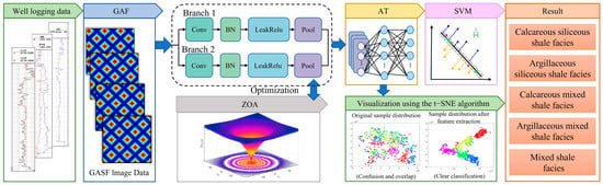
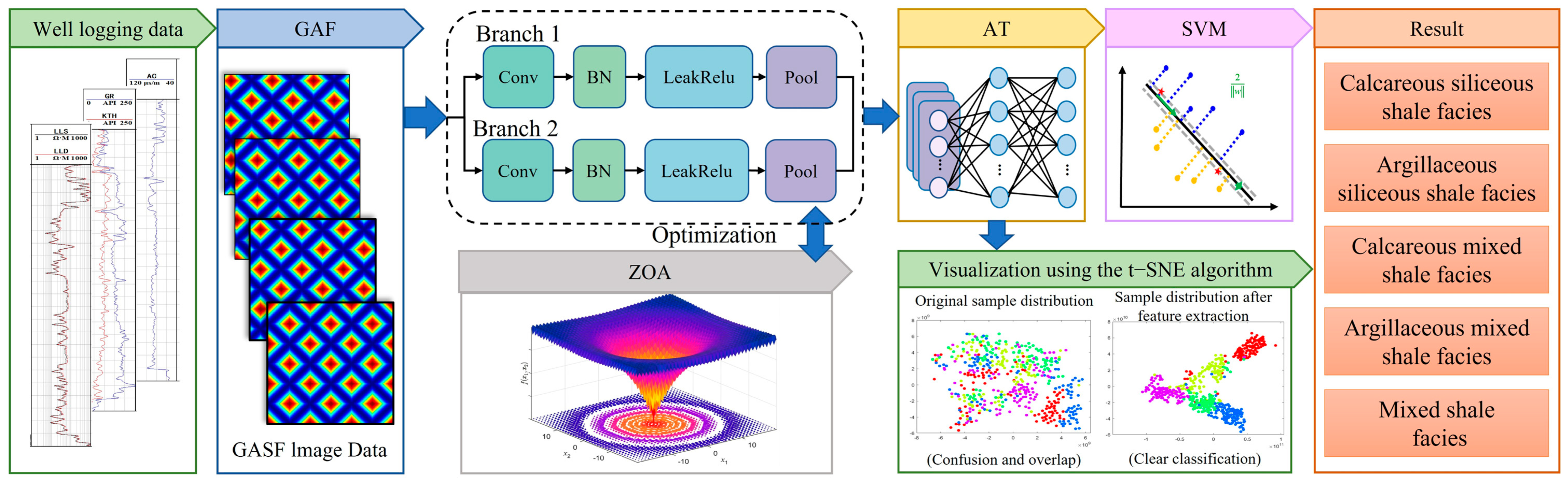
Lithofacies identification in deep shale reservoirs is complicated by heterogeneous rock properties and overlapping well-log responses. This study proposes ZOA-PCNN-AT-SVM, which combines the Zebra Optimization Algorithm (ZOA), parallel convolutional neural networks (PCNN), multi-head attention, and support vector machine classification. The workflow comprises four steps. First, Gramian Angular Field (GAF) mapping converts one-dimensional well-log sequences into two-dimensional images. Second, two parallel convolutional branches extract complementary features. Third, a multi-head attention mechanism reweights the fused features. Finally, ZOA selects the initial learning rate and convolutional kernel sizes, and an SVM classifies the extracted features. The model is evaluated using test wells and separate field applications to assess its performance and limitations.
2. Geological Characteristics and Data Extraction
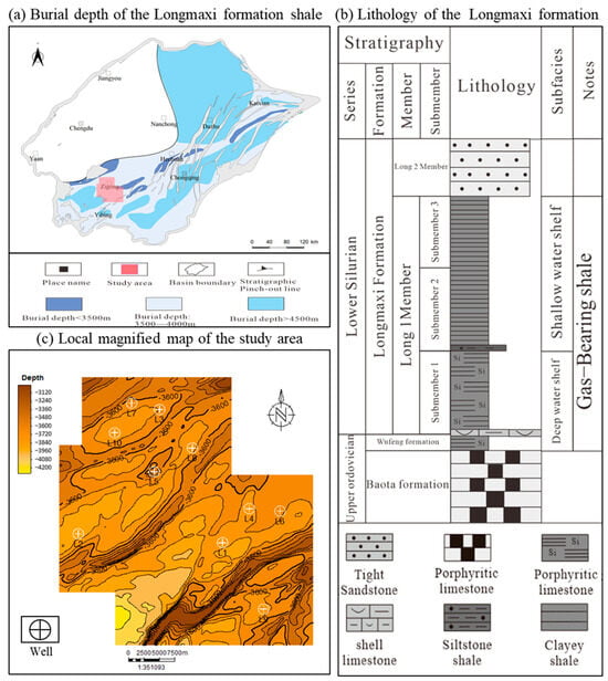
The Sichuan Basin is a major region for marine shale gas exploration and development in China. Located in the western Yangtze Craton, the basin has undergone multiple phases of sedimentary and tectonic evolution. Marine deposition dominated its early history, whereas fluvial and lacustrine deposition became increasingly prevalent from the Late Triassic onward, resulting in successions of marine carbonates and shales as well as continental clastic rocks [23]. The Upper Ordovician Wufeng Formation–Lower Silurian Longmaxi Formation is an important marine shale gas target. The Wufeng Formation and lower Longmaxi Formation were deposited mainly in a relatively deep, low-energy shelf environment, where dysoxic to anoxic bottom waters favored organic-matter preservation and black shale accumulation. As the water shallowed and terrigenous input increased, silty and clay-rich deposits became more abundant in the upper intervals. These changes in depositional environment contributed to vertical variations in mineral composition and shale lithofacies and created favorable conditions for the development of high-quality shale [24,25].
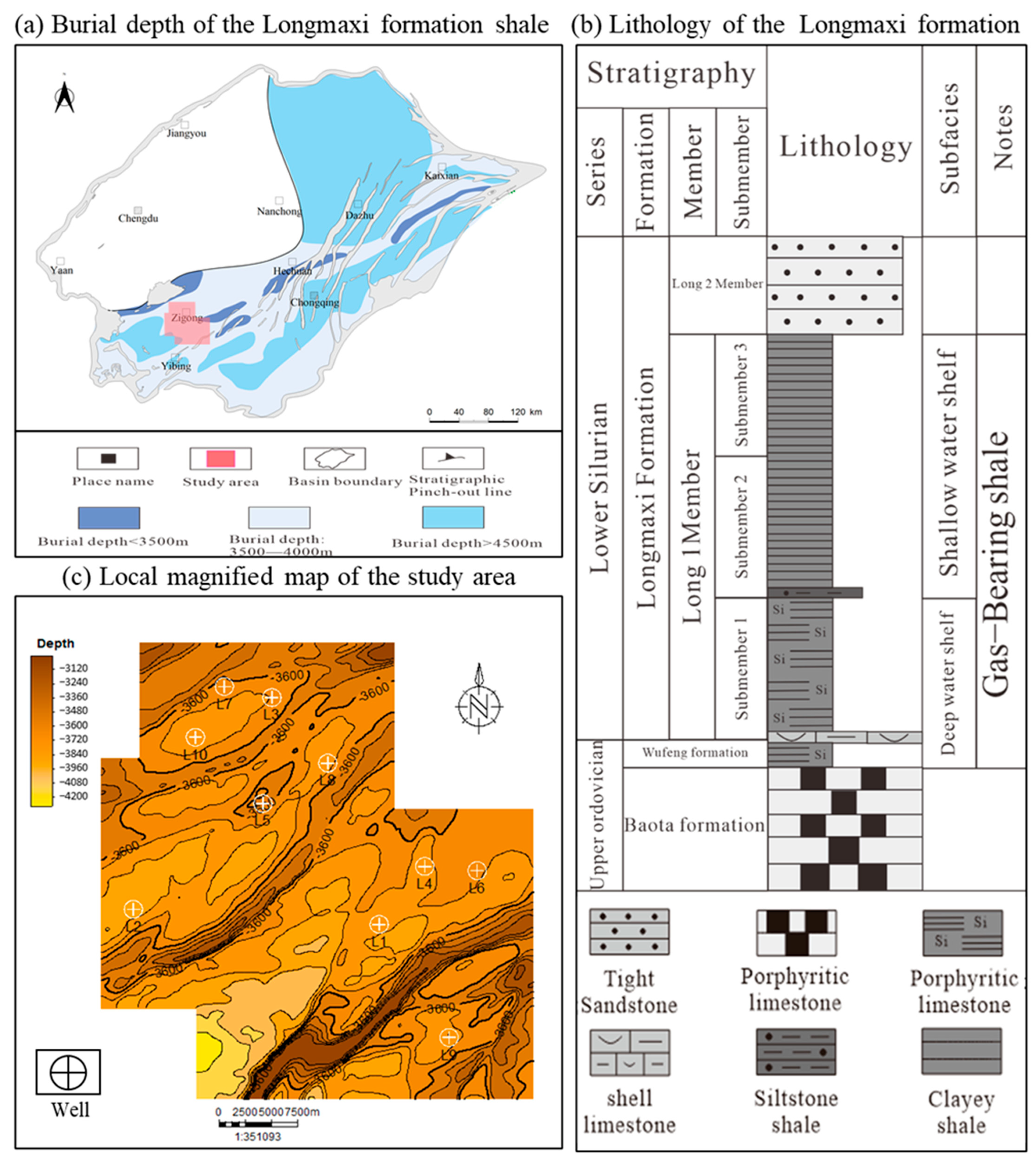
The Zigong area is located in the southwestern Sichuan Basin, within the administrative boundaries of Zigong and Yibin, Sichuan Province. It covers 2458 km2 and is characterized predominantly by hilly terrain (Figure 1). Tectonically, the area occupies a transfer zone at the junction of the Weiyuan and Huayingshan fold systems in southern Sichuan and straddles two tectonic belts: the Zigong low-fold tectonic belt and the Luzhou broom-shaped tectonic belt. The intensity of fold deformation increases progressively from northwest to southeast. Southern Sichuan has undergone multiphase tectonic deformation. Consequently, the strata occur across a broad range of burial depths, from medium-deep to deep, exhibit high thermal maturity, and show marked variations in preservation conditions. These factors have resulted in diverse shale gas reservoir types and complex gas-enrichment patterns.
Figure 1.
Location and structural schematic map of the study area [26,27].
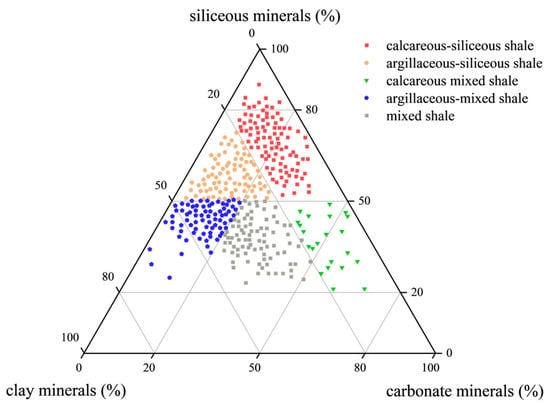
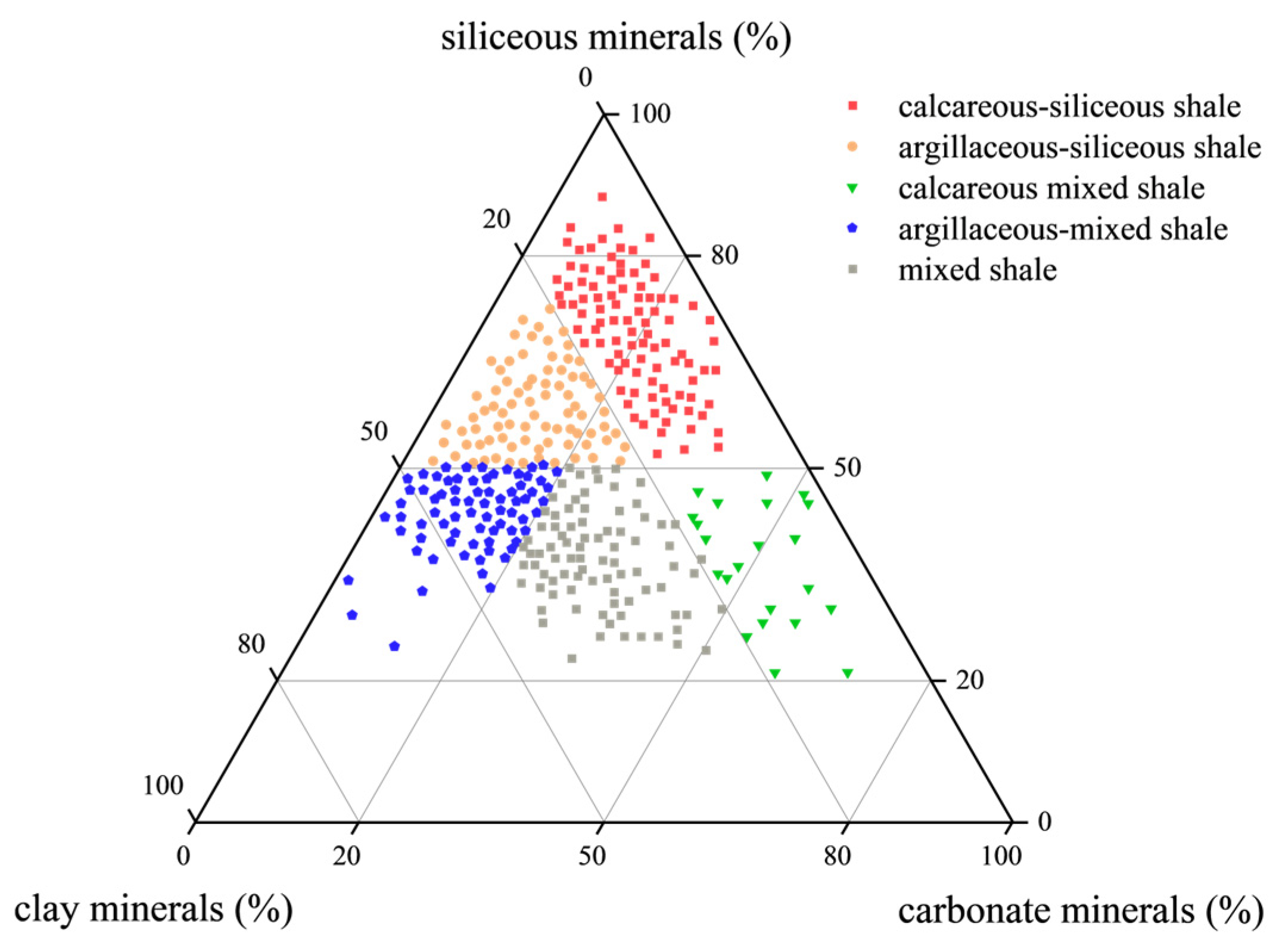
Whole-rock mineralogical analyses were performed on the core samples to determine the mineral composition of the deep shales. A ternary diagram was constructed using siliceous minerals (quartz, feldspar, and pyrite), carbonate minerals (calcite and dolomite), and clay minerals as its three end members. Following an established shale lithofacies classification method and considering the distribution of samples from the study area, a 10% threshold was applied to exclude non-shale lithologies, such as siliceous rock, claystone, and limestone [28]. The remaining samples were plotted on the ternary diagram and classified according to their distribution. Five lithofacies were identified: calcareous siliceous shale (I), argillaceous siliceous shale (II), calcareous mixed shale (III), argillaceous mixed shale (IV), and mixed shale (V) (Figure 2). These five lithofacies encompass the principal combinations and transitional types of siliceous, carbonate, and clay minerals in the study area. Differences in mineral composition are associated with variations in shale pore structure, mechanical properties, and well-log responses. Identifying these lithofacies can therefore inform assessments of reservoir quality.
Figure 2.
Mineral composition ternary diagram.
We compiled core and well-log data from 10 wells in the Zigong block of the deep shale gas region in southern Sichuan. The sampled interval extends from the Wufeng Formation to the first submember of the first member of the Longmaxi Formation, at burial depths of 3500–4500 m. Whole-rock mineral compositions were quantified using X-ray diffraction (XRD), and the samples were assigned to five lithofacies: calcareous siliceous shale (I), argillaceous siliceous shale (II), calcareous mixed shale (III), argillaceous mixed shale (IV), and mixed shale (V) [29,30]. To obtain a class-balanced dataset, 12 labeled samples from each lithofacies were selected from each well. Thus, each well contributed 60 samples, yielding 600 samples in total and 120 samples per lithofacies (Table 1). Based on previous studies and regional geological characteristics, nine well-log variables were selected as input features: acoustic transit time (AC), natural gamma ray (GR), bulk density (DEN), compensated neutron (CNL), potassium (K), uranium (U), thorium (TH), deep laterolog resistivity (RD), and flushed-zone resistivity (RXO). The RD and RXO values were log-transformed to compress their dynamic ranges before model training. The dataset was partitioned at the well level into training, test, and validation sets at a ratio of 7:2:1. Seven wells provided 420 training samples, two wells provided 120 test samples, and one well provided 60 validation samples. All samples from a given well were assigned to the same subset, and the partition was fixed throughout model development. Because each well contributed equal numbers of samples from the five lithofacies, the training, test, and validation sets contained 84, 24, and 12 samples per lithofacies, respectively. The training set was used to fit the models, the validation set to select hyperparameters, and the test set exclusively for final evaluation. This procedure maintained class balance and prevented samples from the same well from appearing in different subsets, reducing the risk of leakage associated with adjacent logging depths.
Table 1.
Part of the original data.
3. Methods
This section describes GAF encoding, parallel convolutional feature extraction, multi-head attention, ZOA-based hyperparameter selection, and SVM classification.
3.1. Visualization of Logging Data Based on GAF
A Gramian Angular Field (GAF) transformation was used to encode one-dimensional well-log sequences as two-dimensional image matrices [31]. The method first normalizes each sequence and maps it from Cartesian coordinates to a polar representation. Trigonometric sum and difference operations then encode relationships between depth-indexed observations. The resulting matrices provide two complementary representations: the Gramian Angular Summation Field (GASF) and the Gramian Angular Difference Field (GADF) [32,33].
Defining the well-logging data X = {x1,x2,…xn} as a time-series array comprising discrete elements, the dataset is subsequently normalized and mathematically formalized via the following governing equations:
where xi denotes the raw well-logging data, and represents the normalized data, constrained within the interval [−1, 1].
The normalized 1D sequence is subsequently projected from the Cartesian domain into a polar coordinate system via the following formulation:
where ϕi denotes the polar angle corresponding to the i sampling point, constrained within the interval [0, π]; ti represents the sequential index; and r defines the polar radius.
By exploiting distinct trigonometric identities, the GAF framework bifurcates into two complementary topological representations: the Gramian Angular Summation Field (GASF) and the Gramian Angular Difference Field (GADF).
GASF is calculated from the cosine of the sum of the polar angles. Its matrix elements are defined as:
GASFi,j = cos(ϕi + ϕj)
Consequently, the corresponding global matrix form is expressed as:
Conversely, the GADF is constructed by evaluating the sine of the difference between the encoded polar angles. Accordingly, the individual elements of this complementary spatial matrix are formulated as:
the corresponding global matrix form is expressed as:
GADFi,j = sin(ϕi − ϕj)
Deep marine shale reservoirs commonly contain millimeter- to centimeter-scale interbeds [34,35]. These may produce rapid changes in natural gamma ray, acoustic transit time, and other well-log responses over short depth intervals. Similar responses can occur in different lithofacies, while the same lithofacies can exhibit different responses [36]. This ambiguity can complicate the identification of thin lithological transitions from one-dimensional signals [37].
The Gramian Angular Field (GAF) overcomes this fundamental bottleneck by retaining the full fidelity of the original logs’ dynamic signatures, effectively eradicating information loss during dimensionality transformation. By mathematically mapping 1D depth-sequential arrays into 2D spatial matrices, GAF intuitively visualizes latent petrophysical correlations, establishing a robust paradigm for the preprocessing and explicit feature visualization of highly complex logging sequences.
3.2. Parallel Convolutional Neural Network
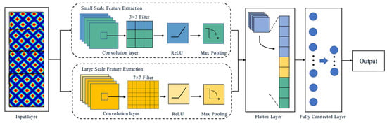
Convolutional neural networks (CNNs) are widely used for image processing and other representation-learning tasks [38,39,40]. Common architectures include convolutional, pooling, and fully connected layers [41]. Parallel convolutional neural networks (PCNNs) use multiple branches to extract and combine complementary features from the input [42].
Within the CNN architecture, the convolutional layer occupies a pivotal role, functioning as the primary engine for feature extraction. Its computational operations not only distill critical latent features from the raw data but also selectively amplify specific target signatures within the original signal while effectively reducing the overall feature dimensionality. Guided by predefined hyperparameters, the convolutional kernel executes a systematic sliding-window operation across the input feature map to generate the output representations [43]. The fundamental mathematical formulation of this convolution is expressed as:
where Wk denotes the convolutional kernel, and Xt−k+1 represents the 1D time-series array.
Subsequent to convolution, the pooling layer functions as a crucial downsampling mechanism that further distills the output features, retaining only the most salient representations while achieving spatial dimensionality reduction [44]. This operation not only significantly mitigates computational overhead but also minimizes the total number of trainable parameters within the model. Pooling mechanisms are predominantly bifurcated into Max Pooling and Average Pooling: the former extracts the maximum activation value within a predefined spatial window, whereas the latter computes the arithmetic mean of the values within that same range. Finally, serving as the terminal component of the architecture, the fully connected layer comprehensively integrates the high-level features extracted through the preceding convolutional and pooling stages to generate the ultimate predictive output (Figure 3).
Figure 3.
Flowchart of the PCNN.
3.3. Multi-Head Self-Attention Mechanism
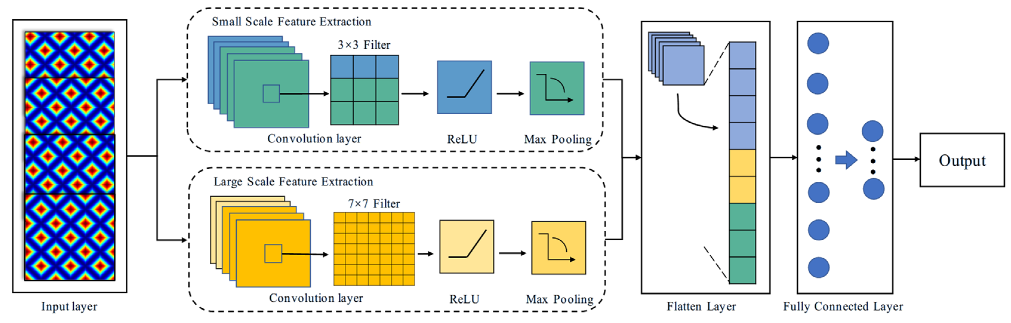
Attention assigns weights to input features according to their contribution to the learned representation. Multi-head self-attention (MHSA) applies attention in multiple learned representation subspaces [45]. The query, key, and value matrices are projected separately for each of the h heads. Attention is computed within each head, and the outputs are concatenated and transformed by a learnable linear projection (Figure 4). The formulation is:
where MultiHead denotes the final output of the Multi-Head Self-Attention mechanism; Concat represents the concatenation operation; headi corresponds to the i individual attention head; and the transformation matrices , , , constitute the learnable weight parameters within the network.
MultiHead(Q,K,V) = Concat(head1,head2,…,headh)W0
Figure 4.
Flowchart of Multi-Head Self-Attention mechanism.
To overcome the profound heterogeneity and complex in situ stress coupling inherent in deep-reservoir lithofacies identification, we integrate a Multi-Head Self-Attention (MHSA) mechanism into the foundational Parallel Convolutional Neural Network (PCNN) architecture. By executing multi-scale feature clustering and attention-driven weighting on raw petrophysical measurements, this framework effectively mitigates the disruptive interference of redundant noise. Consequently, it constructs a highly discriminative feature space for the terminal Support Vector Machine (SVM) classifier, ensuring robust, high-fidelity lithofacies discrimination and accurate classification decisions even within exceedingly complex geological environments.
In the archived implementation, each input image has dimensions of 50 × 40 × 3. The two parallel convolutional branches each contain one convolutional layer with eight filters and same padding, followed by batch normalization, a leaky ReLU activation (slope 0.2), and 2 × 2 max pooling with a stride of one. The branch outputs are concatenated along the second spatial dimension and flattened before entering a self-attention layer configured with one attention head and a key dimension of 50. A fully connected layer with six outputs, a Softmax layer, and a classification layer are used to train the feature extractor. Training uses Adam for 10 epochs with a mini-batch size of 20; the initial learning rate is selected by ZOA, the learning-rate schedule is disabled, and training samples are shuffled every epoch. Network weights are initialized using MATLAB R2024b layer defaults; no custom initializer is specified.
3.4. Hyperparameter Optimization via the Zebra Optimization Algorithm
The Zebra Optimization Algorithm (ZOA), introduced by Trojovska et al. (2022) [46], is a population-based metaheuristic with foraging and defense phases. During foraging, agents update their positions relative to the best-performing current agent, termed the pioneer zebra. During defense, alternative position updates provide additional exploration of the search space. Candidate solutions are evaluated using the specified objective function. The implementation proceeds as follows:
Step 1: Initialization. A population of N agents is initialized randomly within the bounds of a d-dimensional search space. The initial position of agent i is defined as:
where Xi,j denotes the spatial coordinate of the i-th zebra along the j-th dimension; UB and LB define the lower and upper boundaries of the search space, respectively; r is a stochastic scalar uniformly distributed within the interval [0, 1]; and Fi represents the evaluated fitness value for the i-th agent.
Xi,j = LB + r ⋅ (UB − LB)
Fi = F(Xi), i = 1, 2, …, N
Step 2: Foraging Phase (Global Exploration)
The agent with the best current fitness is designated as the pioneer zebra (PZ). Other agents update their positions relative to this agent. A candidate position is accepted only if it improves the objective function; otherwise, the previous position is retained. The update is defined as:
where denotes the newly computed spatial coordinate of the agent subsequent to the foraging maneuver; PZj represents the position of the Pioneer Zebra along the j-th dimension; and I serves as a regulatory control parameter—specifically, a stochastic scalar drawn from the interval [1,2]—introduced to inject stochasticity into the population’s spatial transitions.
Step 3: Defense Strategy Phase (Local Exploitation)
During the local exploitation phase, the algorithm simulates two distinct defensive paradigms governed by a specific probabilistic mechanism. When confronted with a proximal ambush analogous to a lion attack (Ps ≤ 0.5), the agent executes high-frequency, erratic local evasive maneuvers centered strictly around its current spatial coordinates. Conversely, in the event of a sustained long-range pursuit (Ps > 0.5), the population triggers synchronized formation adjustments and collective evasion mechanisms, thereby driving a macroscopic spatial displacement. Within this defensive framework, the positional update equations for the agents are formulated as follows:
where signifies the updated position of the zebra post-defense; t and T correspond to the current iteration and the maximum number of iterations, respectively; R is a random constant within [0, 1]; Ps defines the randomly generated probability value within [0, 1] controlling the defensive strategy selection; and AZj indicates the state of the attacked zebra, with its j-th dimensional component denoted by AZj.
Optimization Problem and Implementation Settings
ZOA optimizes three hyperparameters of the PCNN-AT feature extractor, represented by the decision vector:
where η is the initial learning rate, and k1 and k2 define the square convolutional kernels of the two branches. The learning rate is continuous, whereas the kernel sizes are integer variables; no categorical variable is optimized. The feasible search space is:
x = (η,k1,k2)
= [10−4, 10−2] × {1, 2, 3, 4, 5} × {2, 3, 4, 5, 6}
For each candidate, the PCNN-AT network is trained on the training set, and features extracted from its fully connected layer are used to train an RBF-kernel SVM. The SVM parameters remain fixed at C = 16 and γ = 10−5 and are not included in the optimization vector.
All samples from the same well remain in one subset, and the partition is fixed throughout optimization. For each candidate configuration, the PCNN-AT network and the subsequent SVM are fitted using only the training set. The ZOA fitness function is the classification error of the complete PCNN-AT-SVM pipeline on the 60 samples from the validation well. The optimization objective is:
where yi is the reference lithofacies label derived from XRD analysis, and is the SVM prediction for validation sample i. The indicator function equals one for an incorrect prediction and zero otherwise. Fitness therefore represents the proportion of misclassified validation samples, with lower values indicating better performance. This objective differs from the cross-entropy loss used to train the PCNN-AT network. Accuracy, precision, recall, and F1-score are reported separately as performance measures; precision, recall, and F1-score are not included in the ZOA objective. The same validation well is used throughout the search. The test wells are excluded from model fitting, fitness calculation, and hyperparameter selection and are evaluated only after the best-found configuration has been selected.
ZOA uses two search agents initialized randomly within the specified bounds and runs for a maximum of 10 iterations. Kernel-size coordinates are rounded to integers before network construction. Candidates outside the search bounds are repaired by clipping each coordinate to its corresponding boundary, followed by integer rounding of the kernel sizes. The search terminates after the tenth iteration, without an additional early-stopping criterion. The candidate with the lowest validation error among all evaluated solutions is retained as the best-found configuration.
The complete ZOA optimization and model-training procedure was repeated independently 10 times using random seeds 1–10. At the beginning of each run, the random-number generator was initialized with the corresponding seed to control stochastic operations, including ZOA population initialization, network parameter initialization, and training data shuffling. The well-level training, validation, and test partition remained fixed across all runs. Each run used two ZOA search agents and a maximum of 10 iterations. Candidate configurations were selected exclusively using validation-set classification error, while the test set was reserved for final evaluation.
3.5. The Integrated ZOA-PCNN-AT-SVM Framework
Figure 5 presents the ZOA-PCNN-AT-SVM workflow. First, GAF converts one-dimensional well-log sequences into GASF and GADF images. Second, two parallel convolutional branches extract features from these representations. ZOA selects the learning rate and kernel sizes, as described below. Third, multi-head self-attention reweights the extracted features. Features extracted from the PCNN-AT fully connected layer are supplied to a Support Vector Machine (SVM) classifier, which performs classification using a maximum-margin decision boundary.
Figure 5.
Flowchart of deep shale lithofacies identification based on ZOA-PCNN-AT-SVM.
ZOA optimizes only three hyperparameters of the PCNN-AT feature extractor: the initial learning rate and the convolutional kernel sizes of its two branches, represented by x = (η,k1,k2). The network weights are learned using Adam rather than updated directly by ZOA. The SVM hyperparameters are explicitly fixed at C = 16 and γ = 10−5; they are neither default values nor variables optimized by ZOA. For each candidate configuration, the PCNN-AT network is trained on the training set, and its fully connected features are used to train an RBF-kernel SVM on the same training samples. The resulting PCNN-AT-SVM pipeline is evaluated on the validation well, and its classification error serves as the ZOA fitness value. Thus, although the search variables belong to the feature extractor, candidate selection is based on the performance of the complete classification pipeline. The configuration with the lowest observed validation error is retained, and the test wells are used exclusively for final evaluation. This relationship explains the designation ZOA-PCNN-AT-SVM: ZOA tunes the PCNN-AT hyperparameters, while the SVM is trained with fixed hyperparameters on the resulting features. Furthermore, the t-SNE algorithm visually confirms the model’s classification efficacy by demonstrating highly cohesive intra-class clustering and distinct inter-class boundaries post-dimensionality reduction.
The PCNN-AT feature extractor accepts images of size 50 × 40 × 3. Each of its two parallel branches comprises a convolutional layer with eight filters, batch normalization, a leaky ReLU activation with a negative slope of 0.2, and a 2 × 2 max-pooling layer with a stride of one. The convolutional kernel sizes are determined by ZOA. Same padding is applied to the convolutional and pooling layers to preserve the spatial dimensions. The branch outputs are concatenated and flattened before being supplied to a multi-head self-attention module with two attention heads and a total key dimension of 50, corresponding to 25 dimensions per head. A fully connected layer with five outputs, followed by Softmax and a classification layer, is used for supervised training of the feature extractor. The network is trained using Adam for 10 epochs with a mini-batch size of 20. The initial learning rate is selected by ZOA within the range specified in Section Optimization Problem and Implementation Settings and remains constant during each candidate training run. Training samples are shuffled at every epoch. Features extracted from the five-output fully connected layer are subsequently supplied to an RBF-kernel SVM with fixed hyperparameters C = 16 and γ = 10−5. These SVM hyperparameters are not optimized by ZOA.
4. Results and Discussion
4.1. Logging Data Visualization
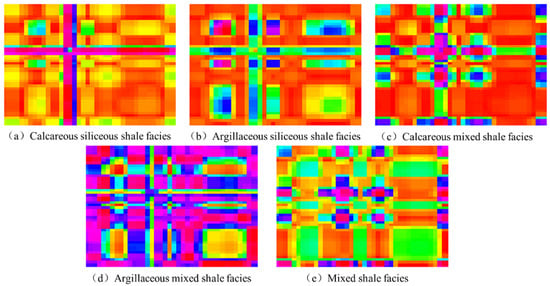
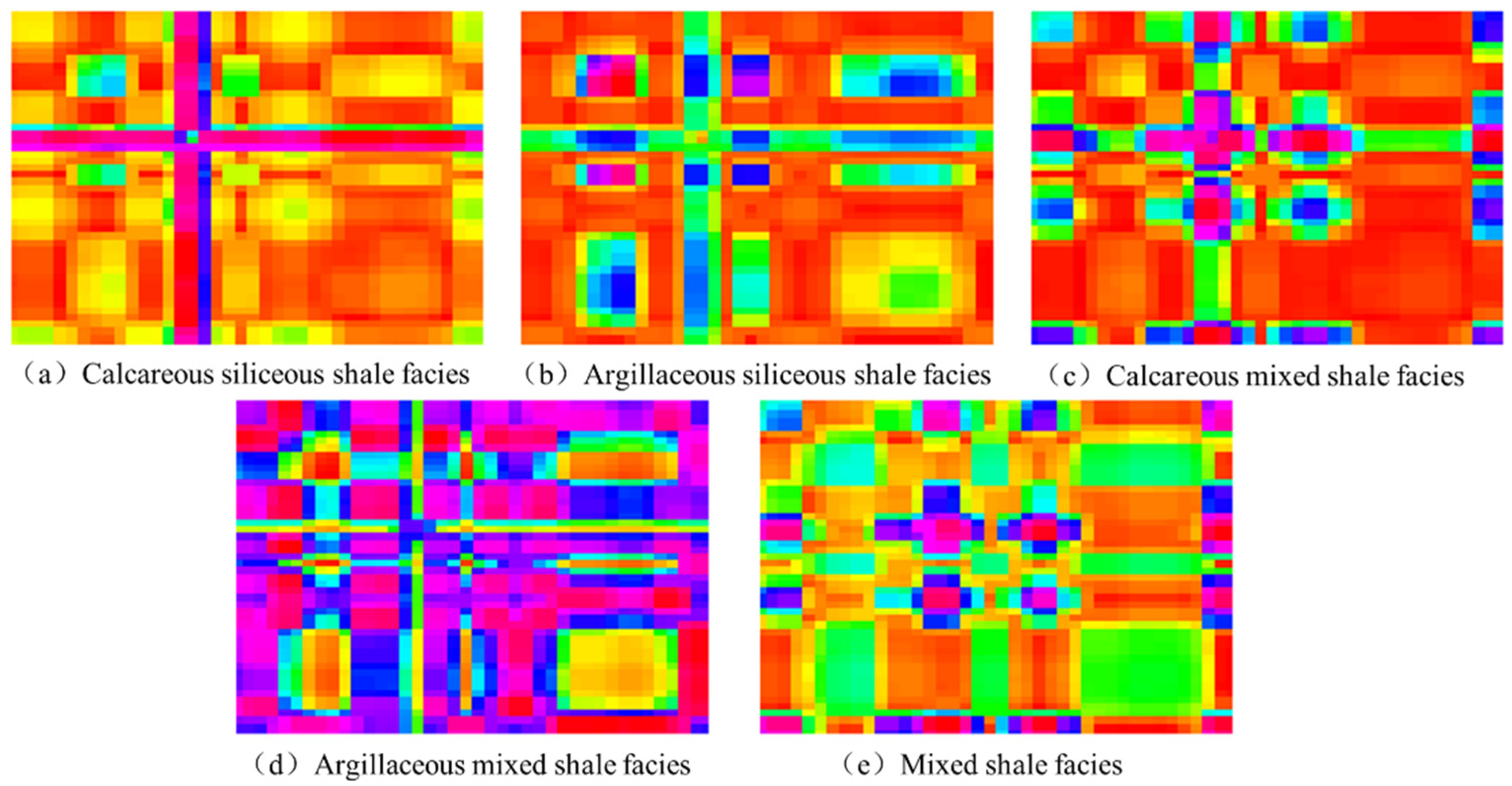
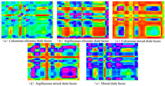
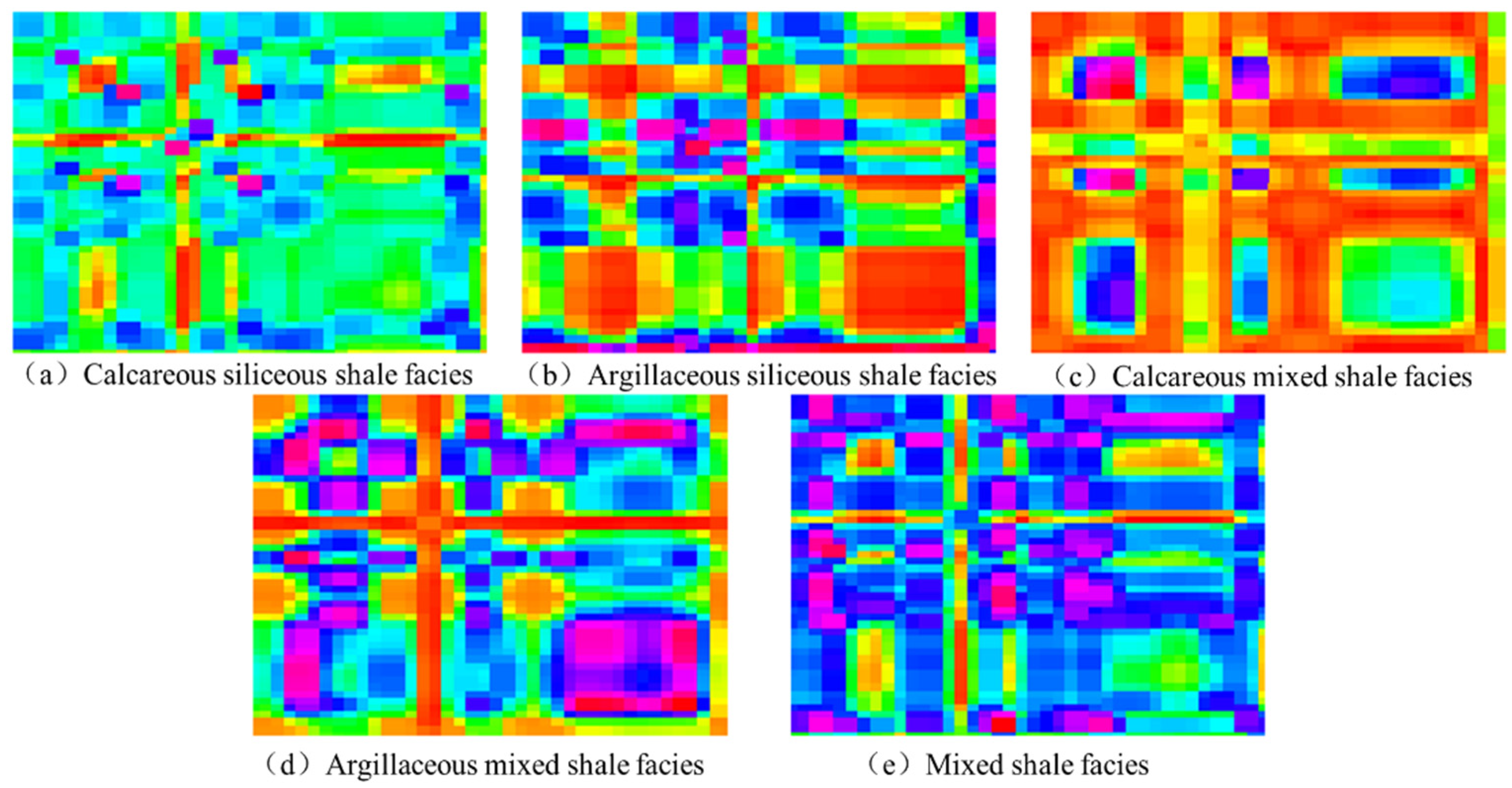
To surmount the engineering bottlenecks dictated by the profound heterogeneity and pervasive thin intercalations of deep shale reservoirs—where conventional 1D well logs inherently fail to resolve micro-scale lithological transitions—this study further leverages the Gramian Angular Field (GAF) transformation for advanced feature reconstruction across all data subsets [47]. By mathematically mapping the rapidly oscillating, discrete logging sequences from the 1D depth domain into 2D Gramian Angular Summation Field (GASF) and Gramian Angular Difference Field (GADF) images (Figure 6 and Figure 7), the latent geological signatures and non-linear dynamics embedded within the raw data are explicitly materialized into highly discriminative visual representations.
Figure 6.
GASF diagram under five lithofacies.
Figure 7.
GADF maps of the five lithofacies.
4.2. Performance of ZOA-PCNN-AT-SVM
Hyperparameter settings influence the performance of the PCNN-AT feature extractor. In this study, ZOA searches for the initial learning rate and the convolutional kernel sizes of the two branches within the predefined bounds. Each candidate configuration is evaluated using the validation-set classification error of the complete PCNN-AT-SVM pipeline. The configuration with the lowest observed validation error is retained as the best-found solution within the specified search budget.
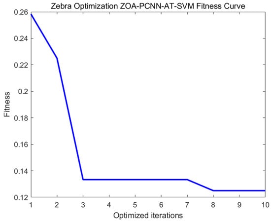
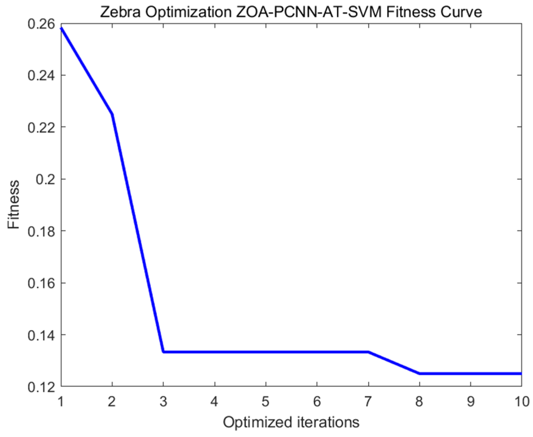
Leveraging the robust global exploration and local-minima escape mechanisms inherent in the Zebra Optimization Algorithm (ZOA), the model conducted an exhaustive search within the high-dimensional hyperparameter space. Figure 8 shows the fitness trajectory of the reported ZOA run. The lowest observed validation error was first reached by approximately the eighth iteration, and the search continued to its preset limit of 10 iterations. The best-found configuration in the reported run used an initial learning rate of 0.00018 and convolutional kernel sizes of 1 × 1 and 2 × 2. The standalone PCNN-AT module had a reported validation accuracy of 85.83%, and its extracted features were subsequently supplied to the SVM classifier. These results describe the observed search behavior and do not establish a mathematical global optimum. To assess sensitivity to stochastic initialization, the complete ZOA optimization and model-training procedure was repeated independently 10 times using random seeds 1–10. Each run used two search agents, random initialization within the bounds defined in Equation (17), and a maximum of 10 iterations. The well-level training, validation, and test partition remained unchanged across runs. Hyperparameter selection was based exclusively on validation-set classification error, with the test set excluded from the optimization procedure.
Figure 8.
Best-so-far validation error across ZOA iterations for the reported run.
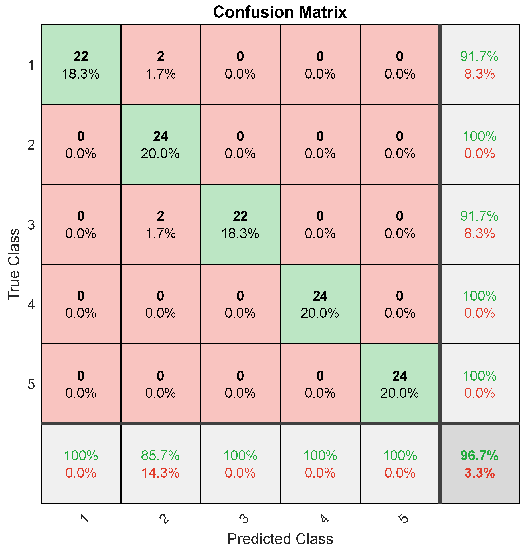
After conversion into 2D images, the data were input to the ZOA-PCNN-AT-SVM model for lithofacies classification. A confusion matrix was used to evaluate classification performance for the five lithofacies. The diagonal entries indicate correct classifications, expressed as sample counts or normalized proportions, depending on how the matrix is displayed. The confusion matrix (Figure 9) shows that most test samples were correctly classified across the five lithofacies. Approximately 14.3% of the argillaceous siliceous shale samples were misclassified. For calcareous siliceous shale, calcareous mixed shale, argillaceous mixed shale, and mixed shale, all test samples were correctly classified.
Figure 9.
Confusion matrix.
In this study, a comprehensive suite of evaluation metrics—namely accuracy, precision, recall, and the F1-score—was employed to systematically assess model performance. The classification results demonstrate that the model correctly classified 116 samples, yielding an overall accuracy of 96.67%. The macro-averaged precision, recall, and F1-score were 97.14%, 96.67%, and 96.72%, respectively. Table 2 reports the corresponding lithofacies-specific metrics. Performance varied among facies: calcareous siliceous and calcareous mixed shale each had a recall of 91.67%, while argillaceous siliceous shale had a precision of 85.71%.
Table 2.
The evaluation index.
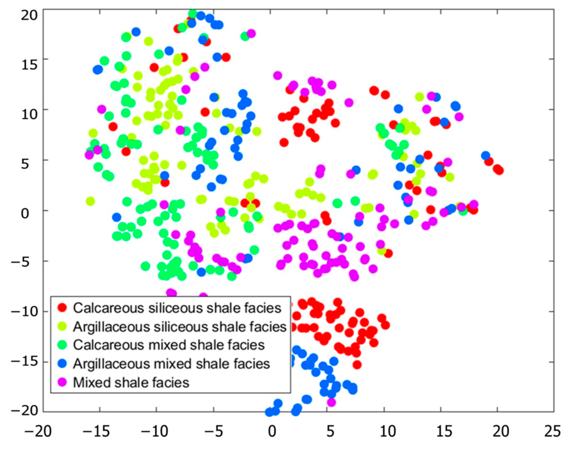
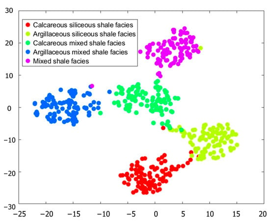
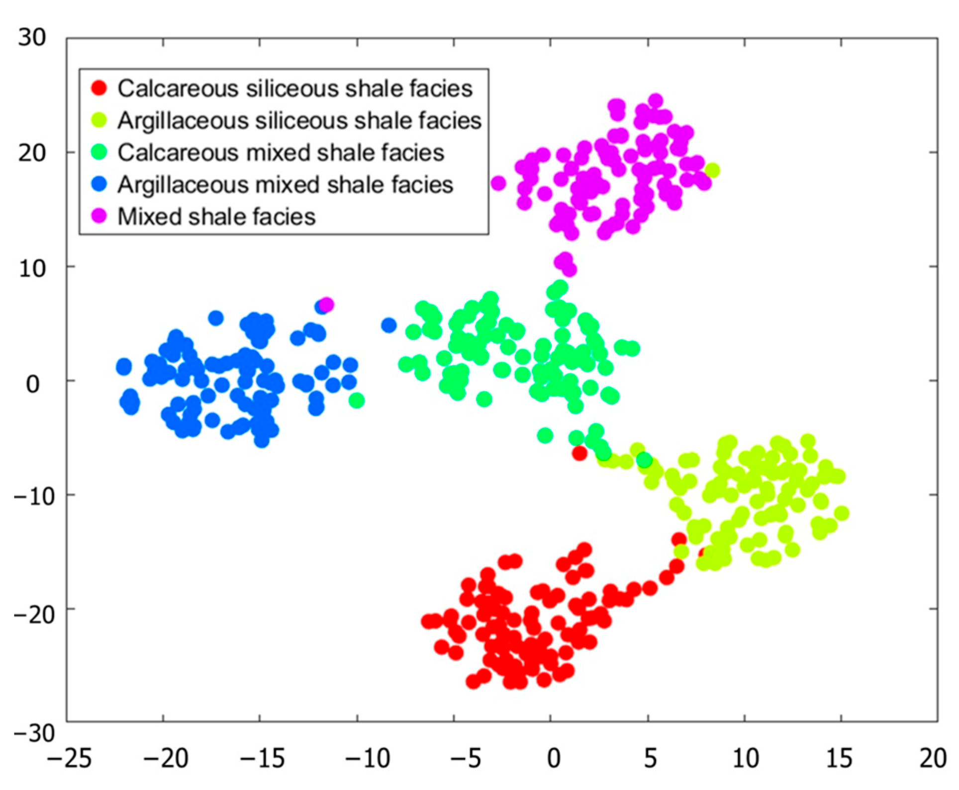
The t-SNE algorithm was used to visualize the raw inputs and extracted features (Figure 10 and Figure 11). The raw inputs showed substantial overlap among lithofacies. In the extracted feature representation, samples formed more distinct clusters, although some dispersion remained for argillaceous siliceous shale.
Figure 10.
Distribution of lithofacies samples before identification.
Figure 11.
Distribution of lithofacies samples after identification.
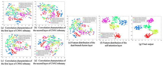
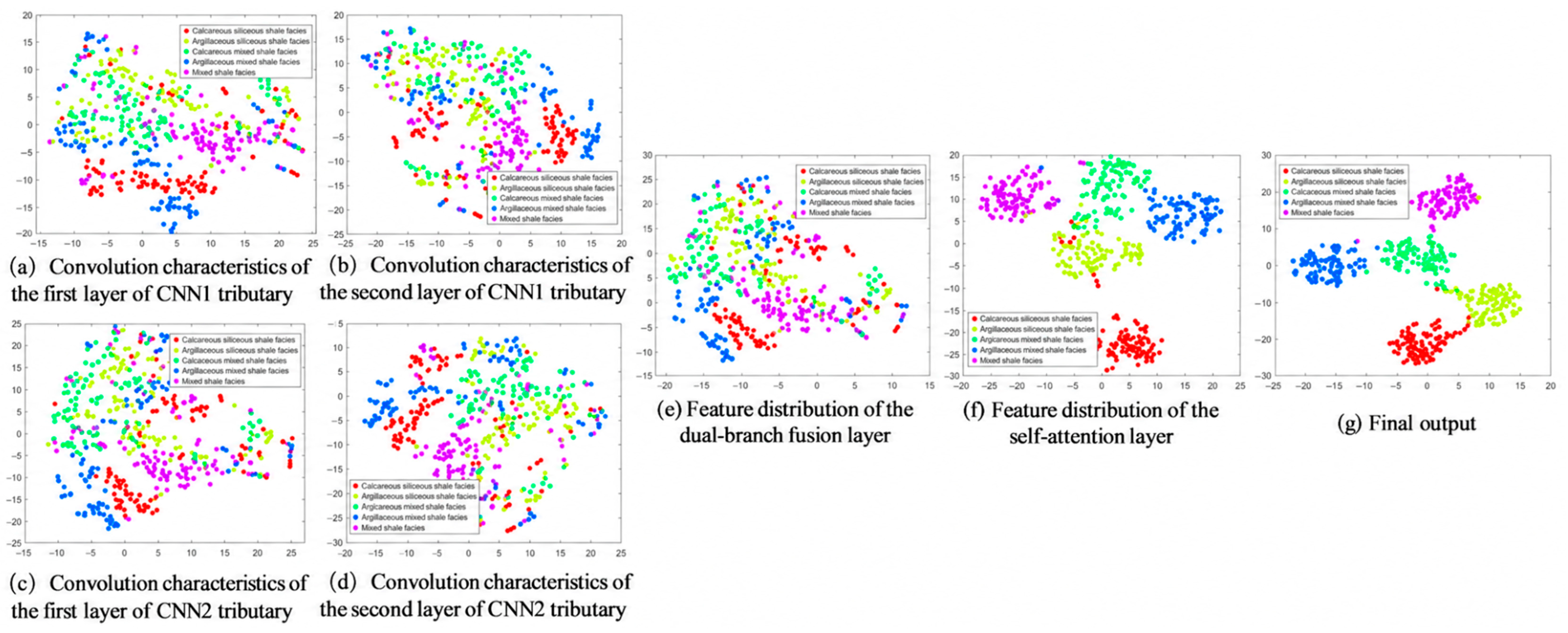
As illustrated in Figure 12a,c, the initial dual-branch convolutional and pooling layers produced dispersed features across the five lithofacies categories. This pattern suggests limited class separability at the early feature-extraction stage. Although subsequent convolutional layers reduced feature overlap between classes (Figure 12b,d), samples remained dispersed. Well-logging data can contain noise and uncertainties associated with instrument characteristics, signal propagation, and acquisition procedures. These factors may contribute to the limited clustering observed after dual-branch feature fusion (Figure 12e). After the introduction of the multi-head attention (AT) mechanism, the features showed clearer separation between lithofacies categories (Figure 12f). This pattern is consistent with AT enhancing discriminative features, although the visualization alone does not establish noise suppression. The final model output showed more compact and distinct lithofacies clusters (Figure 12g). Overall, these visualizations suggest that hierarchical feature extraction and AT provide more discriminative representations than the initial convolutional features in the proposed ZOA-PCNN-AT-SVM architecture.
Figure 12.
Visualization of t-SNE convolution process.
4.3. Comparative Experiment
4.3.1. Ablation Experiment
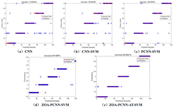
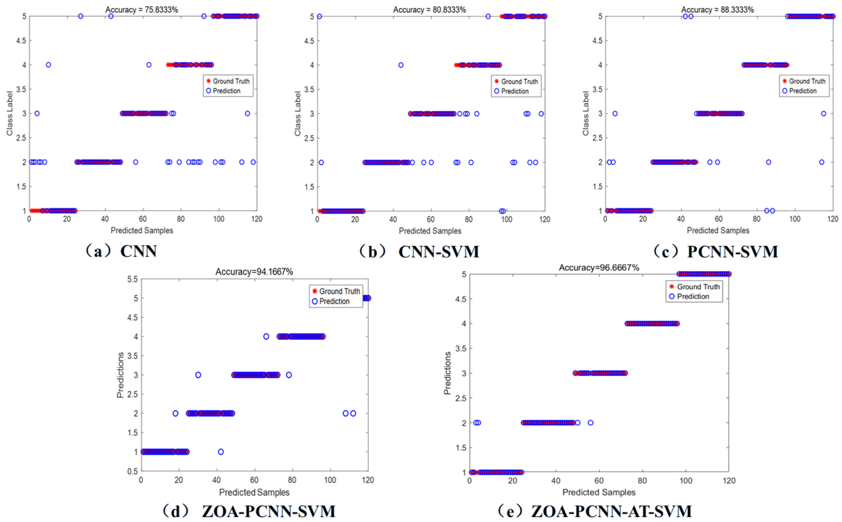
A stepwise ablation study was conducted to assess the contributions of the core modules to deep shale lithofacies identification. These modules comprised the support vector machine (SVM) classifier, dual-branch parallel convolution, multi-head self-attention (MHSA) mechanism, and Zebra Optimization Algorithm (ZOA). Using a common dataset, we compared five model configurations: CNN, CNN-SVM, PCNN-SVM, ZOA-PCNN-SVM, and the full ZOA-PCNN-AT-SVM model. Macro-averaged precision, recall, and F1-score were used to evaluate all models. The predictive scatter distributions in Figure 13a–e illustrate changes in model predictions as successive modules were incorporated. Overall, the results suggest that combining these modules improves lithofacies identification compared with the simpler configurations evaluated in this study.
Figure 13.
Prediction results of different schemes in the ablation experiment test set.
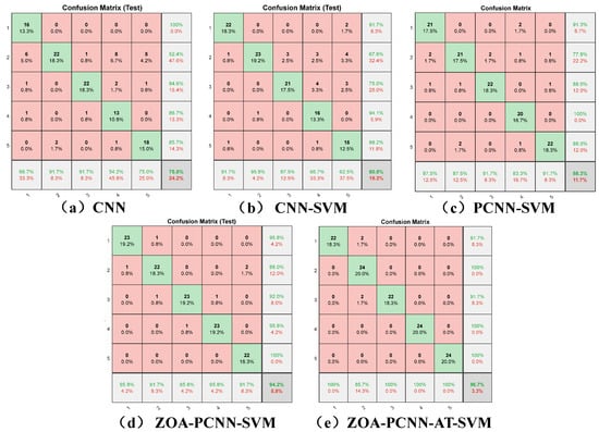
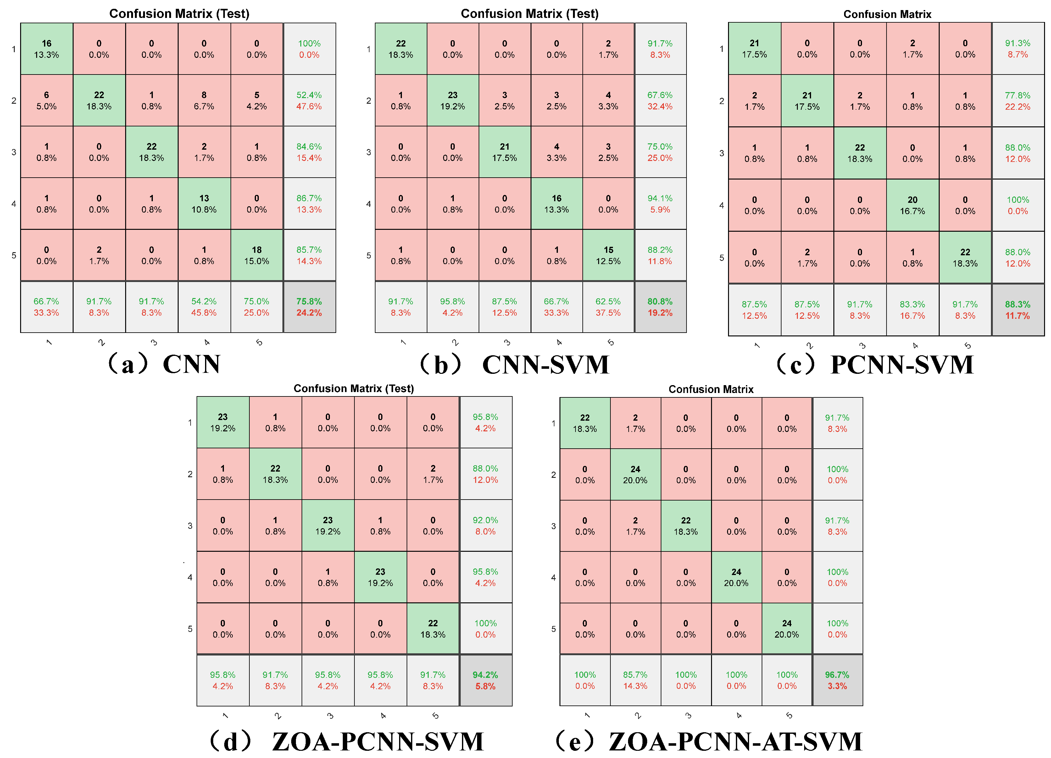
The confusion matrices and evaluation metrics for the compared models are presented in Figure 14 and Table 3. The baseline CNN achieved an accuracy of 75.83%. Replacing the CNN decision layer with an SVM increased accuracy to 80.83%. This improvement suggests that the SVM classifier was better suited to the extracted features in this comparison. With the addition of a parallel dual-branch structure, PCNN-SVM achieved an accuracy of 88.33%. The two branches are designed to capture complementary features from broader trends and local variations in well-log responses. In the full ZOA-PCNN-AT-SVM model, ZOA was used for hyperparameter optimization, while AT reweighted features. The performance gains suggest that this combined architecture improves lithofacies classification on the evaluated dataset.
Figure 14.
Confusion matrices of different models.
Table 3.
Evaluation indicators of different models.
4.3.2. Performance Comparison Between ZOA-PCNN-AT-SVM and Baseline Models
To evaluate the performance of the ZOA-PCNN-AT-SVM model in lithofacies identification, we compared it with four baseline algorithms. These comprised a convolutional neural network (CNN), a long short-term memory (LSTM) network, Light Gradient Boosting Machine (LightGBM), and a standard SVM. Model parameters were optimized using ZOA, and all models were evaluated on the test set. Performance was assessed using accuracy and the macro-averaged values of precision, recall, and F1-score.
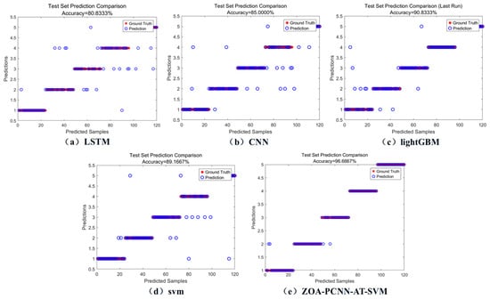
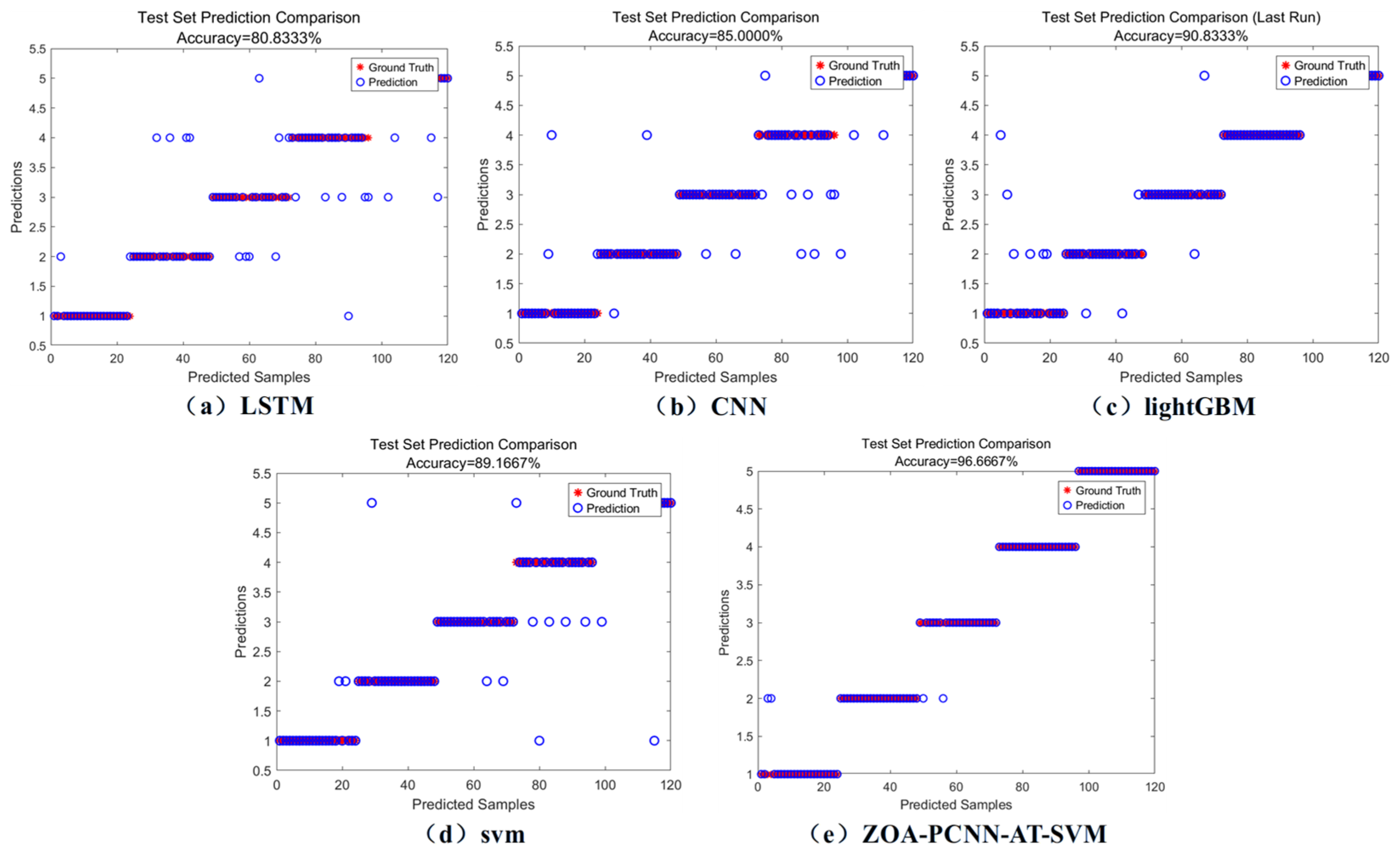
The test-set predictions in Figure 15 illustrate the classification performance of the five models. LSTM and CNN achieved accuracies of 80.83% and 85.00%, respectively, with misclassified samples visible in their scatter plots. SVM and LightGBM achieved higher accuracies of 89.17% and 90.83%, respectively, although some samples remained misclassified. These comparisons suggest that the proposed ZOA-PCNN-AT-SVM model improves lithofacies identification relative to the evaluated baselines. On the same held-out test set, the ZOA-PCNN-AT-SVM model achieved an accuracy of 96.67%, compared with 90.83% for LightGBM, the best-performing baseline. This corresponds to an improvement of approximately 5.8 percentage points.
Figure 15.
Predictive results on the test set.
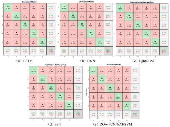
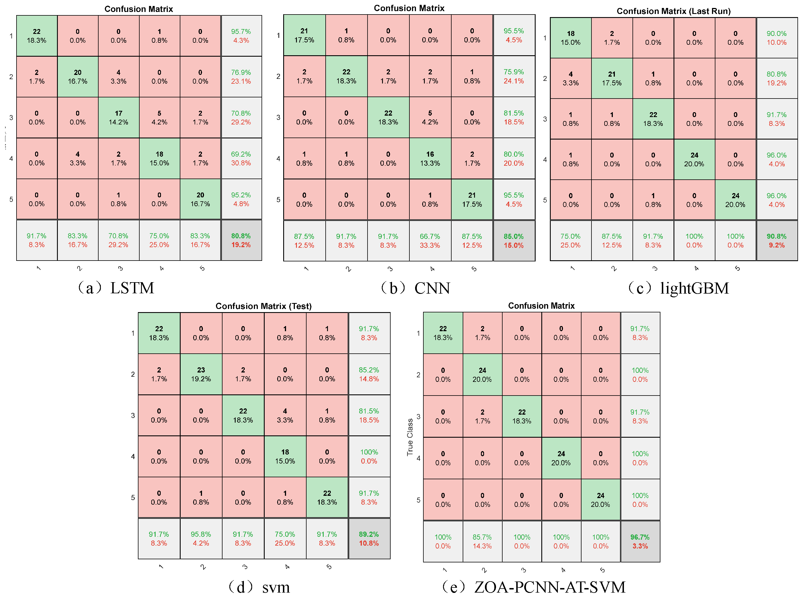
An analysis of the confusion matrices (Figure 16) and evaluation metrics (Table 4) shows that LSTM and CNN achieved F1-scores of 81.07% and 84.93%, respectively. These results suggest limitations of the evaluated network configurations in distinguishing lithofacies with complex petrophysical responses. LightGBM and SVM showed better classification performance than LSTM and CNN in this comparison. Nevertheless, these algorithms remain constrained by pronounced localized confusion and boundary ambiguity among specific lithofacies categories.
Figure 16.
Confusion matrices for the evaluated models.
Table 4.
Performance metrics for the evaluated models.
In deep shale formations, measurement uncertainty and geological complexity can complicate lithofacies identification using well-log data. These factors may contribute to overlapping feature distributions among lithofacies.
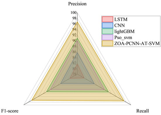
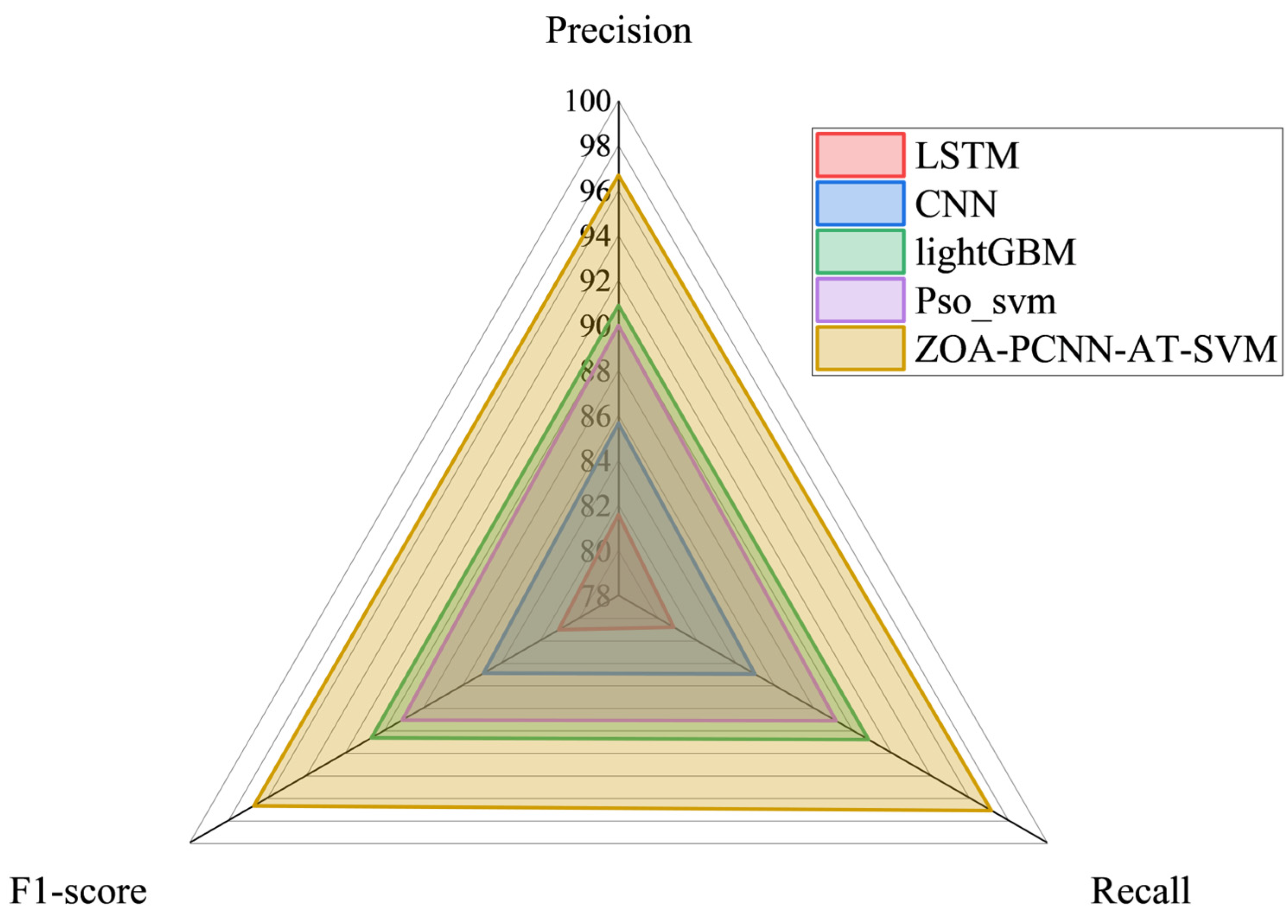
To address this nonlinear multiclass classification problem, the ZOA-PCNN-AT-SVM model combines ZOA-based hyperparameter optimization with multi-head self-attention (MHSA). The results suggest that this combination improves discrimination between lithofacies with overlapping feature distributions (Figure 17).
Figure 17.
Radar chart of evaluation indicators for different models.
4.4. Field Case Validation
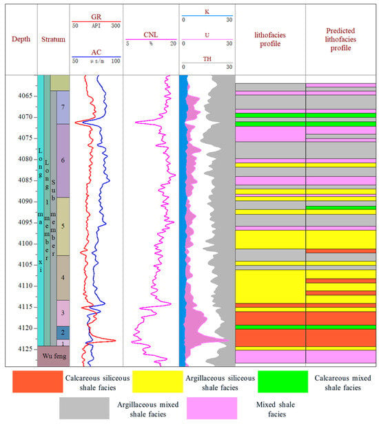
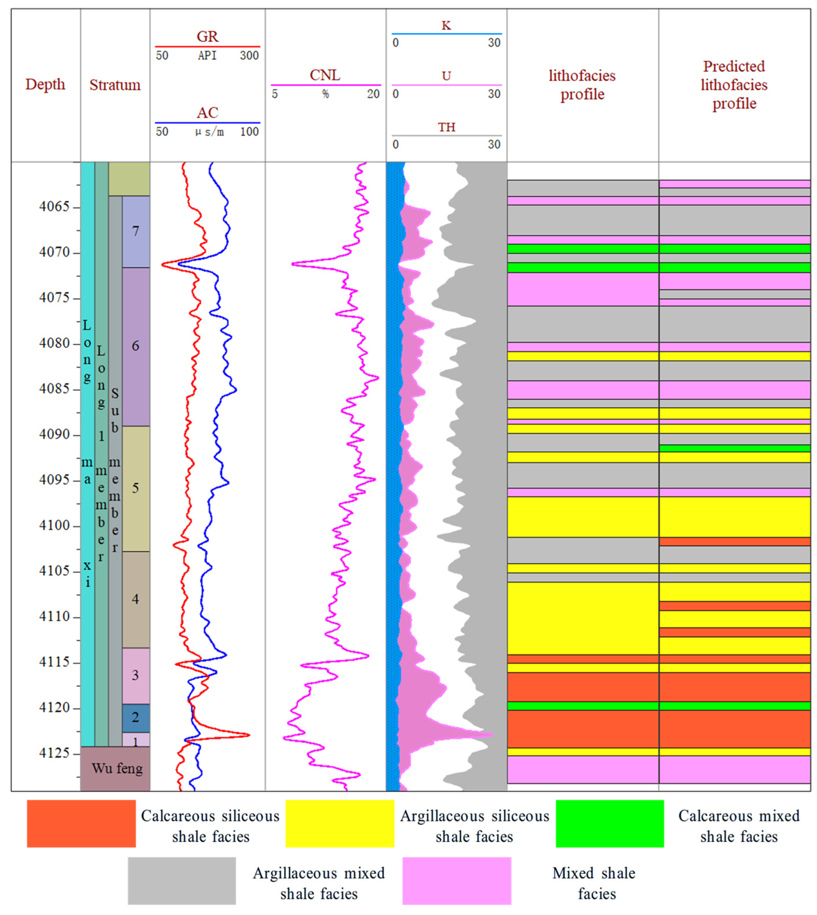
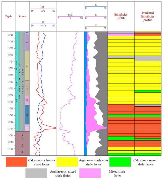
To assess generalization to an independent well, the ZOA-PCNN-AT-SVM model was applied to the target interval of deep shale gas well L1. The interval contains five lithofacies: calcareous siliceous shale, argillaceous siliceous shale, calcareous mixed shale, argillaceous mixed shale, and mixed shale. Calcareous siliceous shale and calcareous mixed shale together account for approximately 10% of the target interval. The predictions in Figure 18 generally agree with the reference lithofacies distributions for four of the five categories. However, predictions for calcareous siliceous shale show discrepancies with its reference distribution.
Figure 18.
Single-well log comparison of identified and actual lithofacies profiles.
Table 5 reports the precision, recall, and F1-score for each lithofacies classified by the ZOA-PCNN-AT-SVM model. Precision exceeded 0.9 for all lithofacies except calcareous siliceous shale, for which it was 0.67. This lower precision indicates that some samples from other lithofacies were incorrectly predicted as calcareous siliceous shale. All five lithofacies had F1-scores above 0.8. The model achieved an overall accuracy of 92.6% on Well L1. This result provides encouraging evidence of its applicability to the evaluated well.
Table 5.
Performance metrics for individual lithofacies.
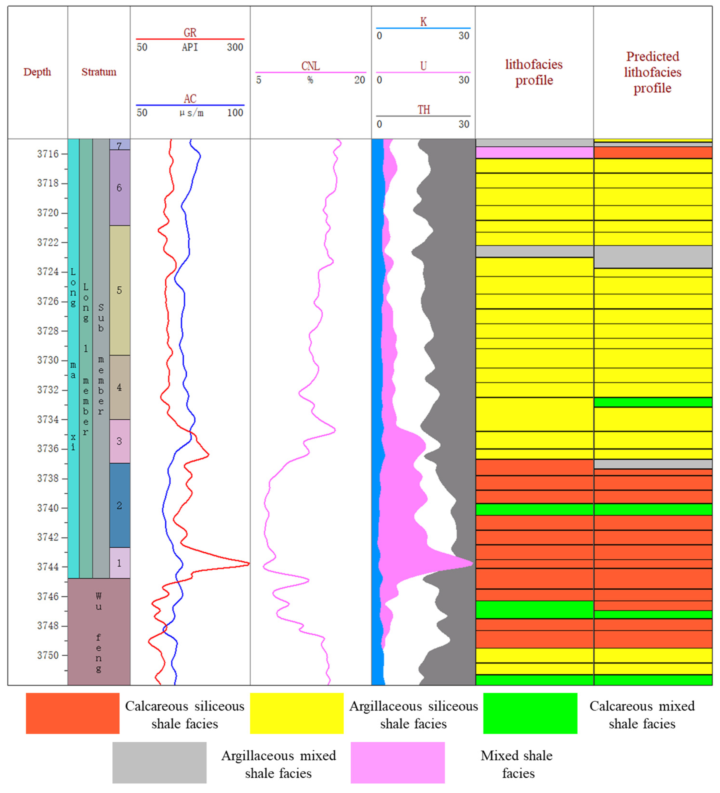
To further evaluate the cross-block applicability of the ZOA-PCNN-AT-SVM model, lithofacies prediction was performed for a deep shale gas well in the LZ block. As shown in Figure 19, the predicted profile generally agrees with the reference lithofacies distribution, capturing the predominance of argillaceous siliceous shale in the upper interval and calcareous siliceous shale in the lower interval. The model achieved an accuracy of 91.7%, although local discrepancies remained in thinner interbeds and near some lithofacies boundaries. The successful application to the evaluated well in the LZ block provides preliminary support for the model’s cross-block applicability.
Figure 19.
Single-well log comparison of identified and actual lithofacies profiles.
Given the limited dataset currently available, this study provides a preliminary evaluation of the proposed framework rather than a comprehensive assessment of its applicability across geological settings. The method is intended to support lithofacies-based reservoir characterization and provide complementary information for future well planning, together with geological and engineering assessments. As additional wells are drilled, new core-derived lithofacies labels and well-log data will be used to independently evaluate predictive accuracy and identify class-specific limitations.
5. Conclusions
Addressing the critical bottlenecks associated with accurate facies recognition in highly heterogeneous deep shale gas reservoirs and complex, non-linear well-log responses, this study introduces and empirically validates an advanced intelligent identification model: the ZOA-PCNN-AT-SVM. By deeply integrating the Zebra Optimization Algorithm, parallel convolutions, and a multi-head attention mechanism, this hybrid framework delivers a robust solution to these geological complexities. The primary findings of this research are as follows:
1. By implementing Gramian Angular Fields (GAF), one-dimensional depth-domain well sequences are profoundly reconfigured into two-dimensional topological feature maps. Synergized with the dual-branch architecture of the Parallel Convolutional Neural Network (PCNN), the framework concurrently captures multi-scale spatial weights. This mechanism facilitates the synergistic integration of high-dimensional features, decisively overcoming the inherent limitations of monolithic neural networks in extracting complex lithological signatures from deep marine shales.
2. To help mitigate acquisition errors and redundant information in empirical well-log data, the Multi-Head Self-Attention (MHSA) mechanism is integrated into the framework. By dynamically weighting the relative contributions of hierarchical features, this module aims to emphasize signatures relevant to lithofacies variations. As indicated by the ablation analysis, this feature weighting yields an accuracy improvement of over 3% under the evaluated experimental conditions, suggesting its potential to improve lithofacies classification in complex subsurface reservoir environments.
3. The ZOA-PCNN-AT-SVM model achieved an accuracy of 96.67% and a macro-F1 score of 96.72% on the held-out test set. A separate evaluation on Well L1 yielded an accuracy of 92.6%, while application to a deep shale gas well in the LZ block achieved an accuracy of 91.7%. The successful application to the evaluated LZ well provides preliminary support for the model’s cross-block applicability. Future work will focus on using the framework to support well planning and on further validating and refining its predictions with newly acquired drilling, core, and well-log data.
Author Contributions
Conceptualization, Y.-Q.L., J.W., C.-Y.L.; Validation, Y.L.; Data curation, J.W. and Y.W.; Writing—original draft, Y.-Q.L.; Writing—review and editing, F.D.; Visualization, Y.-C.T. and R.-H.Z.; Supervision, C.-Y.L. All authors have read and agreed to the published version of the manuscript.
Funding
This research was funded by the Science and Technology Project of China National Petroleum Corporation (CNPC), “Research on Shale Oil and Gas Development Mechanisms and Volumetric Development Technologies,” grant number 2023ZZ08.
Data Availability Statement
The original contributions presented in this study are included in the article. Further inquiries can be directed to the corresponding author.
Conflicts of Interest
Author Jing Wu and Yang Wan were employed by PetroChina Research Institute of Petroleum Exploration & Development. Author Yi Liu was employed by Zhenhua Oil Co., Ltd. Author Run-Hua Zhu was employed by Zhanjiang branch of China National Offshore Oil Corporation (CNOOC). The authors declare that the research was conducted in the absence of any commercial or financial relationships that could be construed as a potential conflict of interest. The authors declare that this study received funding from China National Petroleum Corporation (CNPC). The funder was not involved in the study design, collection, analysis, interpretation of data, the writing of this article or the decision to submit it for publication.
Abbreviations
The following abbreviations are used in this manuscript:
| ZOA | Zebra Optimization Algorithm |
| PCNN | Parallel Convolutional Neural Networks |
| GAF | Gramian Angular Fields |
| SVM | Support Vector Machine |
| MHSA | Multi-Head Self-Attention |
| GASF | Gramian Angular Summation Field |
| GADF | Gramian Angular Difference Field |
| CNN | Convolutional Neural Networks |
References
- Wu, J.; Wang, H.; Shi, Z.; Wang, Q.; Zhao, Q.; Dong, D.; Li, S.; Liu, D.; Sun, S.; Qiu, Z. Favorable lithofacies types and genesis of marine-continental transitional black shale: A case study of Permian Shanxi Formation in the eastern margin of Ordos Basin, NW China. Pet. Explor. Dev. 2021, 48, 1315–1328. [Google Scholar] [CrossRef] [Scilit]
- Wu, J.; Guo, W.; Guo, W.; Zhao, S.; Gou, Q.; Zeng, F.; Liu, Y.; Zou, X.; Wang, Y.; Liu, Z. The petrophysical characteristics and formation mechanism of “sweet spots” for the three-dimensional development of deep marine shale gas: A case study of the first sub-segment of the Longmaxi Formation in the Luzhou block, southern Sichuan Basin. Acta Pet. Sin. 2024, 45, 1219–1233. [Google Scholar] [CrossRef]
- Chen, W.; Wang, B.; Jiang, Z.; Wang, D.; Long, H.; Liu, W.; Liu, D. Characteristics of shale reservoir development under the influence of sedimentary differentiation: A case study of the Cambrian Qiongzhusi Formation in the Deyang-Anyue rift trough of the Sichuan Basin. Nat. Gas. Ind. B 2025, 12, 251–263. [Google Scholar] [CrossRef] [Scilit]
- He, X.; He, G.; Gao, Y.; Zhang, L.; He, Q.; Zhang, P.; Wang, W.; Huang, X. Progress in and research direction of key technologies for normal-pressure shale gas exploration and development. Nat. Gas. Ind. B 2023, 10, 555–569. [Google Scholar] [CrossRef] [Scilit]
- Wang, D.; Jiang, Z.; Du, W.; Liu, D.; Shao, X.; Feng, X.; Chen, Y.; Chen, W.; Yang, Y. Fluid activity characteristics of shallow shale veins in the Wufeng–Longmaxi Formation in the Shixi syncline in northern Guizhou and their significance for shale gas preservation. Nat. Gas. Ind. B 2024, 11, 511–524. [Google Scholar] [CrossRef] [Scilit]
- Tian, M.; Zhu, C.; Li, S.; Xia, Z.; Song, G.; Wang, Y.; Gong, Q.; Li, Y.; Liu, Z. Application of logging lithofacies identification technology of lacustrine carbonate rocks: A case study of Yingxi area, Qaidam Basin. China Pet. Explor. 2023, 28, 135–143. [Google Scholar] [CrossRef]
- Yang, S.; Qiu, L.; Liu, K.; Xu, N.; Yang, Y.; Han, X.; Jiang, J. Lithology logging interpretation model for lacustrine carbonate rocks of the Es4 in Shaojia Sub Sag, Jiyang Depression, Bohai Bay Basin. Xinjiang Pet. Geol. 2015, 36, 708–713. [Google Scholar]
- Cheng, D.; Yuan, X.; Zhou, C.; Tan, C.; Wang, S. Logging-lithology identification methods and their application: A case study on Chang 7 Member in central-western Ordos Basin, NW China. China Pet. Explor. 2016, 21, 117–126. [Google Scholar] [CrossRef]
- Chang, L.I.; Feng, Q.Z.; Liang, D.X.; Feng, Y.H.; Rui, D.C.; Ling, H. Application of the apparent rock fabric number calculation technique in logging identification of the carbonate rock type. Pet. Geophys. 2017, 15, 29–35. [Google Scholar]
- Lyons, M. Ceramic Fabric Classification of Petrographic Thin Sections with Deep Learning. J. Comput. Appl. Archaeol. 2021, 4, 188–201. [Google Scholar] [CrossRef] [Scilit]
- Tang, H.B. Research on Rock Phase Recognition Method Based on Residual Recurrent Neural Network. Master’s Thesis, Northeast Petroleum University, Daqing, China, 2023. [Google Scholar]
- Luo, H.; Lai, F.; Dong, Z.; Xia, X. A lithology identification method for continental shale oil reservoir based on BP neural network. J. Geophys. Eng. 2018, 15, 895–908. [Google Scholar] [CrossRef] [Scilit]
- Liu, Y.; Liu, S.; Ma, Q.; Yao, Z.; She, J. Application of BP Neural Network Method in Shale Lithofacies Recognition of Lucaogou Formation in Sanchanghu Basin. Lithol. Oil Gas. Reserv. 2019, 31, 101–111. [Google Scholar]
- Ameur-Zaimeche, O.; Zeddouri, A.; Heddam, S.; Kechiched, R. Lithofacies prediction in non-cored wells from the Sif Fatima oil field (Berkine basin, southern Algeria): A comparative study of multilayer perceptron neural network and cluster analysis-based approaches. J. Afr. Earth Sci. 2020, 166, 103826. [Google Scholar] [CrossRef] [Scilit]
- Feng, R. A Bayesian Approach in Machine Learning for Lithofacies Classification and Its Uncertainty Analysis. IEEE Geosci. Remote Sens. Lett. 2021, 18, 18–22. [Google Scholar] [CrossRef] [Scilit]
- Zhao, M.; Li, Y.; Fan, C.; Wang, H.; Di, X.; Xu, S. Lithofacies Identification by a Particle Swarm–Optimized Random Forest Algorithm in a Shale Oil Reservoir. SPE J. 2025, 30, 3083–3103. [Google Scholar] [CrossRef] [Scilit]
- Zhang, G.; Wang, Z.; Chen, Y. Deep Learning for Seismic Lithology Prediction. Geophys. J. Int. 2018, 215, 1368–1387. [Google Scholar] [CrossRef] [Scilit]
- Imamverdiyev, Y.; Sukhostat, L. Lithological Facies Classification Using Deep Convolutional Neural Network. J. Pet. Sci. Eng. 2019, 174, 216–228. [Google Scholar] [CrossRef] [Scilit]
- Liu, J.-J.; Liu, J.-C. Integrating Deep Learning and Logging Data Analytics for Lithofacies Classification and 3D Modeling of Tight Sandstone Reservoirs. Geosci. Front. 2022, 13, 101311. [Google Scholar] [CrossRef] [Scilit]
- Liu, Y.; Wu, J.; Zhang, B.; Li, C.; Deng, F.; Chen, B.; Yang, C.; Yang, J.; Tong, K. Lithofacies Identification by an Intelligent Fusion Algorithm for Production Numerical Simulation: A Case Study on Deep Shale Gas Reservoirs in Southern Sichuan Basin, China. Processes 2025, 13, 4040. [Google Scholar] [CrossRef] [Scilit]
- Chen, Y.; Zhang, D. Physics-Constrained Deep Learning of Geomechanical Logs. IEEE Trans. Geosci. Remote Sens. 2020, 58, 5932–5943. [Google Scholar] [CrossRef] [Scilit]
- Li, C.; Wang, X.; Feng, Z.; Song, L.T. Comprehensive identification of microbial dolomite lithofacies based on KNN classification algorithm: A case study of dengsi member in GM area of Sichuan basin. Mar. Orig. Pet. Geol. 2023, 28, 433–440, (In Chinese with English Abstract). [Google Scholar]
- Jiang, S.; Peng, Y.; Gao, B.; Zhang, J.; Cai, D.; Xue, G.; Bao, S.; Xu, Z.; Tang, X.; Dahdah, N. Geology and shale gas resource potentials in the Sichuan Basin, China. Energy Explor. Exploit. 2016, 34, 689–710. [Google Scholar] [CrossRef] [Scilit]
- Zhao, J.; Jin, Z.; Jin, Z.; Wen, X.; Geng, Y.; Yan, C.; Nie, H. Depositional environment of shale in Wufeng and Longmaxi Formations, Sichuan Basin. Pet. Res. 2017, 2, 209–221. [Google Scholar] [CrossRef] [Scilit]
- Guo, W.; Li, X.; Zhang, X.; Lan, C.; Liang, P.; Shen, W.; Zheng, M. Sedimentary microfacies and microrelief of organic-rich shale in deep-water shelf and their control on reservoirs:A case study of shale from Wufeng-Longmaxi formations in southern Sichuan Basin. Acta Pet. Sin. 2022, 43, 1089–1106. [Google Scholar]
- Wang, Y.; Yang, H.; Huang, H.; Fu, L.; Chen, G.; Zhang, H.; Wang, Z.; Guo, K. Geomechanical study of deep shale gas and application in Luzhou block, Sichuan Basin. China Pet. Explor. 2023, 28, 68–83. [Google Scholar]
- Ma, X.; Wang, H.; Zhou, S.; Shi, Z.; Zhang, L. Deep shale gas in China: Geological characteristics and development strategies. Energy Rep. 2021, 7, 1903–1914. [Google Scholar] [CrossRef] [Scilit]
- Wu, J. Microscopic Pore Characteristics and Controlling Factors of Shanxi Formation Shales in the Daning–Jixian Block, Ordos Basin. Ph.D. Thesis, Chengdu University of Technology, Chengdu, China, 2020. [Google Scholar]
- Mou, Y.; Xia, P.; Zhu, L.; Fu, Y.; Wang, K.; Zhao, L.; Qin, C. Geochemical characteristics of the shale gas reservoirs in Guizhou Province, South China. Arab. J. Chem. 2024, 17, 105616. [Google Scholar] [CrossRef] [Scilit]
- Zhao, L.; Xia, P.; Fu, Y.; Wang, K.; Mou, Y. Types of lithofacies in the Lower Cambrian marine shale of the Northern Guizhou Region and their suitability for shale gas exploration. Nat. Gas. Ind. B 2024, 11, 469–481. [Google Scholar] [CrossRef] [Scilit]
- Li, Z.; Chen, Q.; Qian, B.; Niu, Y.; Zhang, Z. Health Diagnosis of Switching Tubes in Grid-connected Inverters Based on Gram Angle Field and Parallel CNN. Electr. Power Autom. Equip. 2024, 44, 153–159. [Google Scholar]
- Wang, Z.; Oates, T. Imaging time-series to improve classification and imputation. In Proceedings of the 24th International Conference on Artificial Intelligence (IJCAI’15); AAAI Press: Washington, DC, USA, 2015; pp. 3939–3945. [Google Scholar]
- Zheng, W.; Lin, R.; Wang, J.; Li, Z.J. Power quality disturbance classification based on GAF and convolution neural network. Power Syst. Prot. Control 2021, 49, 97–104. [Google Scholar]
- Zou, C.; Dong, D.; Wang, Y.; Li, X.; Huang, J.; Wang, S.; Guan, Q.; Zhang, C.; Wang, H.; Liu, H.; et al. Shale gas in China: Characteristics, challenges and prospects (I). Pet. Explor. Dev. 2015, 42, 689–701. [Google Scholar] [CrossRef] [Scilit]
- Liu, Y.; Lai, F.; Xu, H.; Wang, R.; Zhang, X.; Luo, T.; Yang, B. Intelligent identification methods for shale lithology based on the coupling deeply of logging curves. Geol. Sci. Technol. Bull. 2025, 44, 308–320. [Google Scholar]
- Wang, M.; Yang, J.; Wang, X.; Li, J.; Xu, L.; Yan, Y. Identification of Shale Lithofacies by Well Logs Based on Random Forest Algorithm. Earth Sci. 2023, 48, 130–142. [Google Scholar]
- Yang, Y.; Shi, W.; Zhang, X.; Wang, R.; Xu, X.; Liu, Y.; Bai, L.; Cao, S.; Feng, Q. Identification method of shale lithofacies by logging curves: A case study from Wufeng-Longmaxi Formation in Jiaoshiba area, SW China. Reserv. Prop. Oil Gas. 2021, 33, 135–146. [Google Scholar]
- Chen, L.; Zhang, H.; Xiao, J.; Nie, L.; Shao, J.; Liu, W.; Chua, T.-S. SCA-CNN: Spatial and Channel-wise Attention in Convolutional Networks for Image Captioning. In Proceedings of the 30th IEEE Conference on Computer Vision and Pattern Recognition (CVPR 2017), Honolulu, HI, USA, 21–26 July 2017; pp. 6298–6306. [Google Scholar]
- Cheng, G.; Zhou, P.; Han, J. Learning Rotation-Invariant Convolutional Neural Networks for Object Detection in VHR Optical Remote Sensing Images. IEEE Trans. Geosci. Remote Sens. 2016, 54, 7405–7415. [Google Scholar] [CrossRef] [Scilit]
- Krizhevsky, A.; Sutskever, I.; Hinton, G.E.H. ImageNet classification with deep convolutional neural networks. Commun. ACM 2017, 60, 84–90. [Google Scholar] [CrossRef] [Scilit]
- Zhao, Y.; Tang, W.; Nie, Y.; Wang, Z. A classification method of broadband oscillation based on Gram angle difference field and convolution neural network. Power Syst. Technol. 2022, 46, 4364–4372. [Google Scholar]
- Zhu, Z.; Hou, G.; Huang, C.; Sun, G.; Hao, W.; Liang, J. Resource Allocation Algorithm for RIS-Assisted D2D Secure Communication System Based on Parallel CNN. J. Commun. 2022, 43, 172–179. [Google Scholar]
- Li, J. Research on Short-Term Power Load Forecasting Based on Parallel CNN-LSTM Spatial-Temporal Feature Extraction and Enhancement. Master’s Thesis, Nanchang University, Nanchang, China, 2023. [Google Scholar]
- Ma, J.; Wang, F.; Sheng, G.; Qian, Y.; Zhang, J.; Wang, F.; Liu, Y. Fault Diagnosis of GIS Disconnectors Based on Synchronous Extrusion Transformation and Deep Transfer Learning. Electr. Power Autom. Equip. 2024, 44, 218–224. [Google Scholar] [CrossRef]
- Huo, J. Research on Image Semantic Description Algorithm Based on Transformer Architecture. Master’s Thesis, Lanzhou University of Technology, Lanzhou, China, 2024. [Google Scholar]
- Trojovská, E.; Dehghani, M.; Trojovský, P. Zebra optimization algorithm: A new bio-inspired optimization algorithm for solving optimization algorithm. IEEE Access 2022, 10, 49445–49473. [Google Scholar] [CrossRef] [Scilit]
- Li, H.; Huang, X.; Li, L.; Li, F.; Chen, T. Elastic anisotropy differentiation of thin shale beds and fractures using a novel hybrid rock physics model. Solid Earth 2025, 16, 315–332. [Google Scholar] [CrossRef] [Scilit]

Disclaimer/Publisher’s Note: The statements, opinions and data contained in all publications are solely those of the individual author(s) and contributor(s) and not of MDPI and/or the editor(s). MDPI and/or the editor(s) disclaim responsibility for any injury to people or property resulting from any ideas, methods, instructions or products referred to in the content. |
© 2026 by the authors. Licensee MDPI, Basel, Switzerland. This article is an open access article distributed under the terms and conditions of the Creative Commons Attribution (CC BY) license.