


Abstract
Chemical flooding commonly exhibits a non-monotonic oil-production response characterized by an initial increase, peak formation, and subsequent decline. Quantitatively characterizing this response with limited field data remains challenging. This study develops a characteristic-parameter-based framework for reconstructing annual oil-production dynamics during polymer and alkaline–surfactant–polymer (ASP) flooding in Class I reservoirs. The production-response function is parameterized using peak time, maximum annual oil production, and a curve-shape parameter. Empirical regression models are then established to relate these characteristics to reservoir and injection variables. Data from nine polymer-flooding blocks and eight ASP-flooding blocks were used for regression analysis. Model performance was assessed through historical fitting and representative production reconstructions using annual weighted absolute percentage error (WAPE) and cumulative production error (CPE). For the polymer-flooding case, WAPE and CPE were 19.87% and 3.05%, respectively, while the corresponding errors for the ASP-flooding case were 22.85% and 7.37%. The results demonstrate that the framework captures the principal production-response trends and provides quantitative relationships between production characteristics and development conditions. This approach supports interpretable production-response analysis under the investigated reservoir and injection conditions.
1. Introduction
Oil production dynamic prediction is an essential basis for development scheme optimization, production strategy adjustment, and evaluation of enhanced oil recovery (EOR) performance. After long-term water flooding, high-water-cut and ultra-high-water-cut reservoirs usually exhibit increasingly complex remaining oil distributions, limiting further improvement of oil recovery through conventional water flooding. Chemical flooding technologies, including polymer flooding and alkaline-surfactant-polymer (ASP) flooding, can improve remaining oil mobilization by improving the oil–water mobility ratio, expanding swept volume, and reducing oil–water interfacial tension, and have become important EOR techniques for mature oilfields [1,2,3,4,5,6,7]. Field applications have demonstrated that polymer properties, reservoir heterogeneity, and injection strategies significantly affect development performance. Although ASP flooding can enhance displacement efficiency through synergistic effects, its performance is also constrained by system stability and reservoir conditions, requiring prediction methods capable of describing its complex staged production behavior.
Existing oil and gas production prediction methods mainly include decline curve models, probability distribution models, growth curve models, water-flooding characteristic curve methods, and numerical simulation approaches. The exponential, hyperbolic, and harmonic decline models proposed by Arps are among the most widely applied production forecasting methods in petroleum engineering; however, they are mainly suitable for production prediction after entering a relatively stable decline stage [8]. Fetkovich combined decline curve analysis with type curves to improve the identification of different flow regimes, but the method is still primarily focused on decline behavior analysis [9]. The Weibull distribution function provides flexible curve-shape adjustment capability and has been applied to describe production processes with staged variations [10]. Valkó and Lee, Duong, and Clark et al. proposed stretched exponential decline models, fracture-dominated reservoir decline models, and Logistic growth models, respectively, improving the description of unconventional reservoir decline behavior and cumulative production growth processes [11,12,13]. Furthermore, general decline equations established based on production behavior have further expanded the mathematical description capability for complex production dynamics [14].
Although existing approaches can describe different types of production behavior, many classical decline or growth models focus on particular stages of production. Their application to the complete chemical-flooding response, including production increase, peak formation, and subsequent decline, may require appropriate treatment of functional structure, time coordinates, and parameter definitions. Moreover, some empirical model parameters primarily control mathematical curve shape and are not directly related to reservoir development conditions. Consequently, extracting engineering-interpretable production characteristics and establishing quantitative relationships between these characteristics and reservoir or injection conditions represent important directions for chemical-flooding response characterization and parameter estimation.
In recent years, researchers have conducted extensive studies on development indicator prediction and characteristic parameter analysis, establishing various methods for production prediction, reserve evaluation, and development performance assessment [15,16]. Meanwhile, EOR theories and engineering practices have provided important theoretical foundations for chemical flooding applications and development evaluation [17,18]. With the development of polymer flooding and combination flooding technologies, studies have shown that chemical properties, injection parameters, and reservoir conditions jointly influence flooding performance [19,20,21]. Further investigations have demonstrated that polymer viscoelasticity, mobility control capability, and the interfacial tension reduction mechanism of surfactants play important roles in improving sweep efficiency and mobilizing residual oil [22,23,24].
Previous studies have incorporated engineering-interpretable characteristic parameters into the quantitative characterization of chemical-flooding production performance. Hou et al. developed a polymer-flooding production-response model using characteristic cumulative injection points associated with response initiation, peak production, and response termination, together with the peak incremental production. The model was applied to 23 polymer-flooding units in Shengli Oilfield to examine production-response patterns among different reservoir types [25]. Subsequently, Hou et al. combined characteristic-response modeling with genetic algorithms and support vector machines to estimate polymer-flooding production performance from reservoir and development factors [26]. These investigations demonstrate that peak-characteristic-based description and development-variable-based parameter estimation have established precedents. Further methodological investigation is therefore needed to clarify differences in predicted production quantities and independent coordinates and to distinguish retrospective fitting with observed peak constraints from characteristic-parameter estimation based on reservoir and injection information.
With the development of data-driven methods, chemical-flooding performance estimation has expanded from empirical curve fitting toward statistical modeling based on reservoir properties, experimental observations, and field-development data. Amirian et al. investigated data-driven performance forecasting for polymer flooding using experimental and field datasets and incorporated cross-validation into model-configuration assessment [27]. In the related field of petroleum production forecasting, Ruiz Maraggi et al. used leave-one-out and leave-future-out cross-validation to evaluate the predictive performance and uncertainty of rate–time models [28]. Although the reservoir systems and modeling objectives differ, these studies highlight the need to distinguish goodness of historical fit from predictive performance on withheld observations. For chemical-flooding applications involving limited numbers of field blocks, regression sample size, correlations among input variables, and consistent data definitions must also be considered when evaluating characteristic-parameter estimates.
Building on these studies, this work investigates a characteristic-parameter-based framework for analyzing annual oil-production dynamics during polymer flooding and ASP flooding in Class I reservoirs. First, the mathematical relationship between the Weibull-type function and the peak-parameterized production-response function is clarified, while differences in production quantities and independent coordinates between existing incremental-response and annual-production models are identified. Second, empirical relationships are established between peak time, maximum annual oil production, curve shape, and reservoir or injection variables. Finally, historical fitting, representative block reconstruction, and regression-error assessment are used to examine model performance and applicability. The contribution lies in integrating engineering-interpretable production characteristics with parameter-estimation procedures and evaluating their reliability under limited field-data conditions.
2. Materials and Methods
2.1. Field Data Sources and Quality Control
The field data used in this study were derived from historical development records and production databases for polymer and ASP flooding in Class I reservoirs. The raw dataset comprises historical production sequences, reservoir and injection characteristics, and calculated characteristic parameters.
To ensure data reliability, strict quality control procedures were applied. Blocks with incomplete injection-production histories, missing critical parameter records, or evident data anomalies were excluded from the analysis. Based on specific analytical requirements, the data were further organized into two subsets. The first subset, used for model comparison and production reconstruction, consists of 14 blocks with relatively complete production records. The second subset, used for characteristic-parameter regression, comprises 9 polymer-flooding blocks and 8 ASP-flooding blocks, as regression analysis requires stricter completeness of the independent variables. It should be noted that these subsets are derived from the same pool of field blocks rather than representing three independent datasets; specifically, the 14 blocks used for production reconstruction include those 9 and 8 blocks used for regression.
2.2. Weibull-Type Production Response Model
The Weibull-type function is an empirical statistical model that has been widely applied for describing non-monotonic production behavior. In this study, it was used as a representative existing production-response model for comparison. The production rate and cumulative production can be expressed as:
where a is the amplitude coefficient; b is the shape parameter of the Weibull model and controls the curve shape; c is the scale parameter of the Weibull model; Qo(t) is the oil production rate at time t, t/d; and Np(t) is the cumulative oil production up to time t.
As expressed in Equation (1), its production rate depends on an amplitude parameter, a power-law term, and an exponential attenuation term. For positive values of the shape parameter b and scale-related parameter c, the function increases initially, reaches a single maximum, and subsequently declines.
Equation (2) represents the time integral of Equation (1), assuming that cumulative production is measured from the same time origin. The asymptotic cumulative production is ac/(b + 1), provided that the model assumptions and parameter constraints are satisfied. When time is measured in days, the parameter c has units of time raised to the power b + 1, so that the exponential argument is dimensionless. The characteristic time scale is therefore c1/(b+1).
The peak production time of Equation (1) can be obtained by differentiation:
which gives:
Therefore, although the Weibull-type function does not directly use peak production parameters as independent variables, its peak characteristics can be derived from the fitted model coefficients.
The cumulative production in Equation (2) is obtained by integrating Equation (1):
which provides the relationship between instantaneous production behavior and accumulated production.
Considering key development nodes such as chemical-flooding response time, peak time, and injection end time, previous studies established an oil production prediction model for chemical flooding:
where ∆Q(x) is monthly incremental oil production; ΔQmax is the maximum monthly incremental oil production, t/month; x0 is the injected pore volume (PV) at which chemical flooding begins to be effective; xm is the injected PV at the peak response of chemical flooding; and b is the curve shape parameter. The model requires xm > x0 and is applied over the response interval x ≥ x0. The response reaches its maximum value ΔQmax at x = xm.
Introducing the normalized injection coordinate:
Equation (3) can be expressed as:
The end-of-injection coordinate may define the practical evaluation interval but is not an independent parameter in Equation (3). Consequently, the function does not automatically constrain incremental production to zero at the injection endpoint.
2.3. Peak-Parameterized Oil Production Response Model
The chemical-flooding oil production curve can be divided into a response rise stage, a transition stage near the peak, and a post-peak decline stage. To characterize this behavior, an empirical unimodal response function was adopted for the parameterized representation of annual oil production dynamics.
where Q(t) denotes the oil-production response corresponding to annual reporting period t, which is represented by a numerical time coordinate referenced to the selected starting period. a, b, and c are model constants. The constraints a > 0, b > 0, and c > 0 ensure a positive response with a unique internal maximum. The coordinate t in Equation (4) is treated as a dimensionless numerical time variable referenced to a one-year interval, ensuring consistent definitions of the exponential and power terms.
Q(t) = atbec(1 − t)
Normalizing Equation (4) by the peak time and maximum production response gives:
After peak normalization, Equation (4) shares the same mathematical form as Equation (3). However, their fundamental distinction lies in the physical parameterization. Equation (4) explicitly incorporates peak time and maximum annual oil production as characteristic parameters. This structural difference provides practical engineering value: the shape parameter b can be directly regressed against reservoir and injection variables. This study focuses on estimating peak and shape parameters via operational variables to construct a semi-empirical prediction method for chemical flooding, advancing from curve fitting to physically constrained prediction.
For the three unknowns in the formula, two different solution methods can be used, and their production fitting accuracies are different.
Method 1: Least-squares method. The undetermined coefficients a, b, and c in the formula are fitted using actual production data.
To determine the model constants a, b, and c, let c = b/tm. Then the above equation can be processed as follows:
where
β = b
Equation (5) can then be expressed in linear regression form:
where
lnQi = α + βXi
When the peak time tm is fixed, the transformed predictor Xi is independent of candidate values of the unknown shape parameter b. Therefore, the intercept α and slope β can be estimated directly by ordinary least squares, without searching for the value of b that maximizes the correlation coefficient. The regression objective is:
The model parameters a, b, and c are finally determined:
b = β
This method requires positive production values and positive time coordinates. Missing observations are excluded, and zero-production values cannot be directly logarithmically transformed. The fitted coefficients must also satisfy the unimodal requirement b > 0. Because the objective is defined in logarithmic production space, this method does not necessarily minimize annual absolute production errors in the original production scale.
Method 2: Peak-Constrained Parameter Estimation Method. According to the formula derivation, the relationship among the undetermined coefficients a, c, and b is obtained. The undetermined coefficient b is selected by minimizing the error of recoverable reserves.
To determine the model parameters a, b, and c, differentiating both sides of Equation (4) with respect to t gives:
When dQ/dt = 0, production reaches the maximum Q = Qmax, that is:
Substituting this into the improved oil production model gives the maximum production formula:
According to the formula derivation, the undetermined coefficients a and c can be calculated from the undetermined coefficient b:
These relationships indicate that once peak time and maximum production are specified, the remaining unknown is the shape parameter b. To avoid cancellation between positive and negative annual production residuals, the revised retrospective fitting procedure employs weighted absolute production error as its objective:
Here, Ω denotes the set of valid annual observation periods. Under the specified observed peak constraints, the reconstructed production is given by:
The optimal shape parameter is determined by:
For recalculation using the available production records, the parameter search may be restricted to 0.05 ≤ b ≤ 30, followed by bounded numerical optimization. This interval represents a numerical search constraint rather than a universal physical range for the shape parameter. When a revised objective is adopted, the associated retrospective fitting parameters and errors must be recalculated consistently.
Importantly, this procedure directly uses the observed peak time and maximum annual oil production of the target block. Its zero theoretical peak error therefore follows from the imposed constraints and does not demonstrate the ability to predict the peak characteristics of an unseen block independently. Genuine block-level prediction requires estimation of all three characteristic parameters from reservoir and injection information.
2.4. Variable Normalization
The main characteristic parameters of the improved oil production model include peak time tm, maximum annual oil production Qmax, and shape coefficient b. These parameters are jointly affected by reservoir conditions, pre-production development status, and chemical agent injection mode. The main variables include chemical agent injection rate v, PV/a; water cut before chemical flooding fw0, %; cumulative polymer dosage Mp, mg/L·PV; cumulative surfactant dosage Ms, mg/L·PV; formation permeability k, mD; effective thickness h, m; and well-pattern density characterization parameter D, wells/km2.
Chemical-flooding input variables have different units and orders of magnitude. Direct linear regression may cause variables with large orders of magnitude to occupy a large weight in parameter solution. Therefore, logarithmic normalization is used to convert the original variables into dimensionless variables:
where xg is the geometric mean of variable x; Sx is the standard deviation of the logarithmic relative variable; and n is the number of samples.
The characteristic parameters are expressed by an exponential empirical formula:
where Y is the characteristic parameter to be predicted; Yg is the geometric mean of the characteristic parameter; βj is the regression coefficient; and p is the number of variables entering the empirical formula.
The exponential form can ensure that the predicted peak time, maximum annual oil production, and shape parameters are positive, and it reduces the influence of parameter unit changes on formula coefficients.
2.5. Polymer-Flooding Characteristic-Parameter Regression Model
For Class I oil-layer polymer-flooding blocks, pre-production water cut, cumulative polymer injection, effective thickness, permeability, and chemical-flooding injection rate were selected as regression independent variables. These variables represent the pre-production development status of the block, the scale of chemical agent input, reservoir physical properties, and injection intensity, respectively, and have good field data availability. On this basis, multiple regression was used to analyze the relationships among variables. The formulas are:
In Equation (22), the coefficients of cumulative polymer dosage, permeability, and effective thickness are all positive, indicating that within the existing sample range, when the scale of chemical agent action and effective reservoir thickness increase, the oil production peak time generally shifts later. Equation (23) indicates that cumulative polymer dosage and effective thickness are important influencing factors of maximum annual oil production. The shape parameter in Equation (24) reflects the peak width of the oil production curve and the post-peak decline rate, and its variation is jointly affected by injection intensity, pre-production development status, and reservoir permeability.
2.6. ASP-Flooding Characteristic-Parameter Regression Model
ASP flooding simultaneously involves polymer viscosity enhancement, surfactant interfacial-tension reduction, reaction between alkali and acidic components of crude oil, and emulsification and migration. Its production dynamics are affected not only by reservoir conditions and injection intensity but also by chemical-agent compatibility, adsorption loss, alkali consumption, scaling, and system stability. The oil production response is more complex than that of polymer flooding. This study adopts the same characteristic-parameter modeling approach as that for polymer flooding. Cumulative polymer injection, cumulative surfactant injection, injection rate, pre-production water cut, effective thickness, permeability, and well-pattern density were selected as regression independent variables. A characteristic-parameter regression model for Class I oil-layer ASP flooding was established. The formulas are:
Equation (25) indicates that within the existing sample range, when injection rate and cumulative surfactant dosage increase, the oil production peak time generally shifts later; when cumulative polymer dosage and permeability increase, the peak response is relatively earlier. After the surfactant reduces oil–water interfacial tension, the migration of the low-interfacial-tension system in the reservoir and the mobilization of remaining oil may last for a longer time, thus delaying the oil production peak. Equation (26) shows that maximum annual oil production generally increases with cumulative polymer dosage and well-pattern density, and is negatively correlated with pre-production water cut. The absolute value of the regression coefficient of cumulative surfactant dosage is relatively small, indicating that after controlling for polymer dosage, pre-production water cut, and well-pattern density, its independent statistical contribution to maximum annual oil production is limited. This negative coefficient reflects a partial regression relationship under the combined action of multiple factors, and it does not mean that increasing surfactant dosage will necessarily reduce oil production. In Equation (27), the shape parameter b is jointly affected by reservoir permeability, effective thickness, well-pattern density, and cumulative surfactant dosage. The regression coefficient corresponding to cumulative surfactant dosage is small, indicating that its influence on peak width is weaker than that of reservoir physical properties and well-pattern conditions. As the surfactant action time is prolonged, the oil production response may be distributed over a longer time range, making the peak shape flatter.
2.7. Model Evaluation and Error Metrics
To distinguish the interpretations of different model results, production-response assessment was divided into three settings: retrospective peak-constrained fitting, in-sample characteristic-parameter-based reconstruction, and held-out block prediction assessment.
Retrospective fitting reconstructs historical production using observed peak constraints from the target block. In-sample reconstruction estimates characteristic parameters using regressions calibrated with data that include the target block. Held-out assessment excludes the target block from regression training. Only the third setting, when information leakage is adequately controlled, can assess internal cross-block predictive performance.
The weighted absolute percentage error (WAPE) was used to quantify annual oil-production deviations:
where T denotes the number of valid annual reporting periods, and Qipred and Qiobs represent predicted or reconstructed and observed production in period i, respectively. Production quantities must have consistent units and reporting definitions, and the observed cumulative production over the evaluation period must be positive.
The cumulative production error (CPE) was used to quantify the net difference between predicted and observed cumulative production over the same evaluation period:
WAPE and CPE characterize different aspects of model performance. WAPE uses absolute annual residuals and does not permit cancellation of positive and negative deviations. In contrast, CPE measures the net cumulative discrepancy, which may be small when annual errors compensate for one another. Consequently, a low cumulative production error alone does not establish high accuracy in annual production prediction.
For leave-one-block-out assessment, standardization parameters and regression coefficients must be calculated using training blocks only. The characteristic parameters and production sequence of the held-out block are then estimated independently. If the predictor combinations were previously selected using the complete dataset, the resulting assessment must be identified as exploratory leave-one-block-out evaluation with fixed predictor specifications, rather than fully nested validation of the complete model-selection procedure.
3. Results
3.1. Comparison of Parameter-Estimation Methods
To evaluate the fitting performance of different parameter-estimation procedures for chemical-flooding production dynamics, two least-squares specifications and a peak-constrained derivative method were compared using historical production observations. The three approaches differ in their peak constraints and parameter-estimation procedures. Their peak-production, annual production, and cumulative production errors are summarized in Table 1.
Table 1.
Fitting errors of different parameter solution methods.
As shown in Table 1, the two least-squares specifications yielded annual production errors of 20.11% and 18.70%, with corresponding cumulative errors of 8.17% and 6.13%. The peak-constrained derivative method produced annual and cumulative errors of 17.02% and 3.90%, respectively. Because this method directly incorporates the observed peak characteristics to determine the peak location and amplitude, its zero peak error follows from the parameter constraints. Accordingly, comparisons among these procedures should emphasize annual production deviations outside the constrained peak and overall cumulative production discrepancies.
3.2. Regression Performance of Production Characteristic Parameters
Empirical regression relationships were established for peak time, maximum annual oil production, and production-curve shape using reservoir and injection characteristics from Class I polymer-flooding and ASP-flooding blocks. The polymer-flooding and ASP-flooding datasets comprised nine and eight blocks, respectively. The statistical performance of the characteristic-parameter regressions was evaluated using the coefficient of determination, in-sample mean relative error, and leave-one-block-out cross-validation error, as summarized in Table 2 and Table 3.
Table 2.
Fitting results of empirical formulas for polymer-flooding characteristic parameters.
Table 3.
Fitting results of empirical formulas for ASP-flooding characteristic parameters.
The polymer-flooding shape-parameter regression exhibited relatively high in-sample goodness of fit, with an R2 of 0.930, a mean relative error of 4.82%, and a leave-one-block-out error of 9.42%. In comparison, the peak-time and maximum-production regressions yielded R2 values of 0.649 and 0.523, with corresponding leave-one-block-out errors of 18.81% and 16.82%, respectively. These results indicate that the selected variables characterized in-sample variation in curve shape more effectively, whereas appreciable unexplained variability remained in peak time and maximum annual production.
The ASP regressions exhibited notable differences between in-sample goodness of fit and held-out block errors. The peak-time and maximum-production models achieved R2 values of 0.942 and 0.969, respectively, but their corresponding leave-one-block-out errors reached 15.04% and 30.58%. In particular, the coexistence of high in-sample goodness of fit and appreciable held-out error for maximum annual production indicates sensitivity to the composition of the training dataset. The shape-parameter regression yielded an R2 of 0.786 and a leave-one-block-out error of 19.19%, also indicating uncertainty in cross-block parameter estimation.
Overall, the characteristic-parameter regressions exhibited different degrees of statistical stability for the two flooding systems. Given the limited number of independent blocks, high in-sample coefficients of determination do not necessarily correspond to low cross-block prediction errors. In addition, correlations among some explanatory variables in the ASP regressions may increase coefficient uncertainty. Accordingly, the empirical coefficients primarily characterize statistical associations between reservoir or injection variables and production-response characteristics within the investigated datasets.
3.3. Comparison of Historical Production-Response Fitting
To compare the ability of different production-response models to characterize chemical-flooding production dynamics, the Weibull-type model, the existing modified production-response model, and the peak-constrained parameterized model were applied to 14 block-labeled historical production records. Each method was evaluated using its corresponding parameter-estimation procedure. The annual and cumulative production errors are presented in Table 4. Because the methods differ in their peak constraints and calibration procedures, the comparison primarily characterizes historical fitting performance under the respective estimation conditions.
Table 4.
Comparison of retrospective fitting errors among different oil production response models.
Across the 14 block-labeled records, the mean annual WAPE values of the Weibull-type model, modified production-response model, and peak-constrained model were 47.58%, 25.43%, and 20.65%, respectively. Their corresponding mean cumulative errors were 5.66%, 13.64%, and 5.37%. The median annual WAPE values were 46.51%, 25.03%, and 19.09%, while the sample standard deviations were 12.56%, 5.41%, and 3.85%, respectively. Under the considered retrospective fitting conditions, the peak-constrained model exhibited lower and less dispersed annual production errors.
Annual and cumulative production errors did not exhibit identical patterns across the models. Some fitted responses reproduced cumulative production relatively closely while retaining appreciable deviations in individual reporting periods. This indicates that cumulative production agreement alone is insufficient to evaluate production-response models; their ability to characterize the rising stage, peak formation, and post-peak decline must also be considered.
3.4. Production Reconstruction of Representative Field Blocks
3.4.1. Polymer-Flooding Case
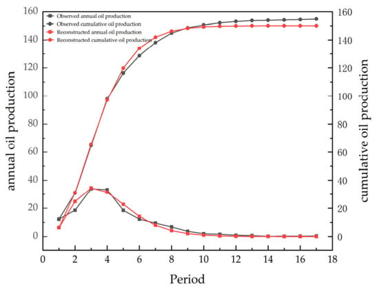
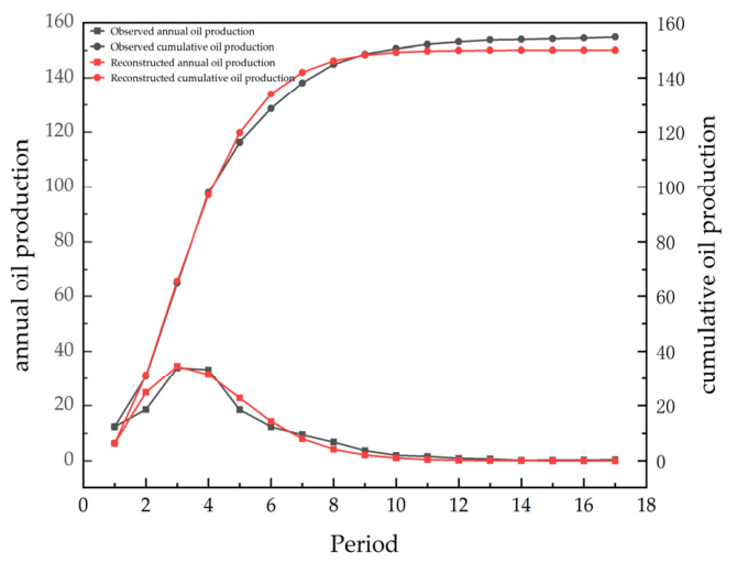
The Xing 4–5 Central polymer-flooding block was selected as a representative application for annual production reconstruction using empirically estimated characteristic parameters. With a peak time of 3.19, maximum annual production of 34.73, and a curve-shape parameter of 3.59, annual and cumulative production were reconstructed over 17 reporting periods. The model parameters and error metrics are summarized in Table 5, and the observed and reconstructed production profiles are compared in Figure 1.
Table 5.
Production reconstruction results for the polymer-flooding block.
Figure 1.
Observed and reconstructed annual and cumulative oil production for the Xing 4–5 Central polymer-flooding block.
Over the 17 periods, observed cumulative production was 154.84, compared with reconstructed cumulative production of 150.11, yielding an annual WAPE of 19.87% and a cumulative CPE of 3.05%. As shown in Figure 1, the reconstructed response captured the overall increase, peak, and subsequent decline in oil production, although deviations remained in certain reporting periods. The cumulative production error was substantially lower than the annual production error, indicating differences between estimating the overall production magnitude and reproducing annual production allocation.
3.4.2. ASP-Flooding Case
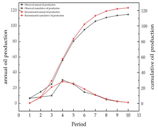
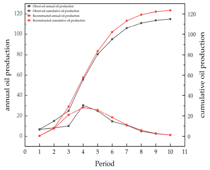
To examine the application of the framework to ASP flooding, the Xing 3–4 East Block II block was selected as a representative case. Using a peak time of 4.20, maximum annual production of 28.56, and a curve-shape parameter of 6.01, annual and cumulative production were reconstructed over 10 periods. The model parameters and error statistics are presented in Table 6, with the corresponding production profiles shown in Figure 2.
Table 6.
Production reconstruction results for the ASP-flooding block.
Figure 2.
Observed and reconstructed annual and cumulative oil production for the Xing 3–4 East Block II ASP-flooding block.
Over the 10 periods, observed cumulative production was 114.96, whereas reconstructed cumulative production was 123.44, resulting in an annual WAPE of 22.85% and a cumulative CPE of 7.37%. Figure 2 shows that the model captured the major characteristics of peak production and subsequent decline, although appreciable deviations occurred during the production-growth stage and certain post-peak periods. Reconstructed cumulative production exceeded the observed value, indicating a positive net accumulation of annual production deviations.
4. Discussion
Chemical-flooding production responses generally exhibit distinct stages, including production increase, peak formation, and post-peak decline. The major contribution of this study is not the construction of an entirely new mathematical curve family, but the introduction of an engineering-oriented peak-constrained parameterization framework based on existing unimodal response functions. By constraining the decay-related parameter using the peak time tm, the model parameters are transformed from purely mathematical fitting coefficients into interpretable characteristic parameters, including peak occurrence time, maximum production capacity, and response persistence. Furthermore, empirical relationships between these characteristic parameters and reservoir/injection variables enable the transition from production-response description to block-level characteristic prediction.
The comparison among different models indicates that cumulative production error alone is insufficient for comprehensively evaluating production-response models. Because production curves exhibit strong temporal variations, annual production error reflects the capability of a model to reproduce production growth and decline stages, whereas cumulative production error represents long-term consistency. Therefore, both annual WAPE and cumulative CPE were adopted in this study to provide complementary evaluations. It should be noted that a low cumulative error may also result from compensation between positive and negative deviations during different periods; thus, cumulative agreement does not necessarily indicate accurate reproduction of annual production dynamics.
The empirical regressions of characteristic parameters were developed using a limited number of field blocks, including nine polymer-flooding blocks and eight ASP-flooding blocks. Because chemical-flooding performance is simultaneously affected by injection scale, reservoir heterogeneity, well-pattern characteristics, and operational conditions, uncertainty in regression coefficients is inevitable under small-sample conditions. Therefore, the empirical relationships established in this study should be regarded as statistical associations applicable to similar development conditions rather than universal physical laws. The results also indicate that high in-sample fitting accuracy does not necessarily guarantee reliable block-level prediction, highlighting the importance of considering sample coverage and variable correlations.
The representative block applications further demonstrate the applicability of the proposed framework for production-response reconstruction. For the Xing 4–5 Central polymer-flooding block, the model achieved an annual WAPE of 19.87% and a cumulative CPE of 3.05% over 17 annual observations. For the Xing 3–4 East Block II ASP-flooding block, the corresponding values were 22.85% and 7.37% over 10 observations. The reconstructed profiles captured the overall unimodal production trends for both flooding methods, although deviations remained during certain periods. These deviations may originate from production adjustments, reservoir heterogeneity, and complex chemical interactions that are not fully represented by the current empirical parameter system.
It should be emphasized that the block evaluations conducted in this study represent dynamic reconstruction and characteristic-parameter application based on available production data rather than fully independent long-term forecasting validation. Due to the limited number of available field blocks, a large-scale independent test dataset could not be established. Future studies should incorporate additional reservoirs with different geological conditions and development stages and perform broader external validation to further improve model generalization.
5. Conclusions
- (1)
- A peak-constrained parameterization framework was proposed for chemical-flooding production dynamics. The method characterizes unimodal production responses using peak time, maximum production, and response-shape parameters, and further establishes empirical relationships between characteristic parameters and reservoir/injection variables. Its major advantage lies in improved engineering interpretability rather than increased mathematical complexity.
- (2)
- Model comparisons demonstrate that annual and cumulative production errors represent different aspects of model performance, reflecting short-term dynamic variations and long-term production consistency, respectively. Therefore, both indicators should be considered for evaluating chemical-flooding production-response models.
- (3)
- The empirical regressions established using limited field blocks can support characteristic-parameter estimation for representative cases; however, their reliability is affected by sample size, variable correlations, and block heterogeneity. Therefore, these relationships should be applied within development conditions comparable to those used for calibration.
- (4)
- Field applications demonstrate that the proposed framework can reproduce the major production trends of polymer flooding and ASP flooding. The polymer-flooding case achieved an annual WAPE of 19.87% and cumulative CPE of 3.05%, while the ASP-flooding case achieved 22.85% and 7.37%, respectively. The framework provides a practical tool for production-response analysis and characteristic evaluation under limited-data conditions.
Author Contributions
Conceptualization, D.W.; Software, J.X.; Validation, J.W. and J.Y.; Data curation, Y.G.; Writing—original draft, J.X.; Validation, J.Y.; Supervision, D.W.; Funding acquisition, D.W. All authors have read and agreed to the published version of the manuscript.
Funding
This research was funded by the National Natural Science Foundation of China (Grant No. 52604045).
Data Availability Statement
The data supporting the conclusions of this study are included within the article. The raw data were provided by the oilfield operator and cannot be publicly shared due to data ownership. A limited portion of the processed data may be available from the corresponding author upon reasonable request.
Conflicts of Interest
Author Jianmin Yan was employed by Oilfield Management Center, No. 11 Oil Production Plant, Daqing Oilfield. The remaining authors declare that the research was conducted in the absence of any commercial or financial relationships that could be construed as a potential conflict of interest.
Abbreviations
The following abbreviations are used in this manuscript:
| ASP | Alkaline–Surfactant–Polymer |
| EOR | Enhanced Oil Recovery |
| PV | Pore Volume |
| WAPE | Weighted Absolute Percentage Error |
| CPE | Cumulative Production Error |
References
- Seright, R.S.; Wang, D. Polymer flooding: Current status and future directions. Pet. Sci. 2023, 20, 910–921. [Google Scholar] [CrossRef] [Scilit]
- Scott, A.J.; Romero-Zerón, L.; Penlidis, A. Evaluation of Polymeric Materials for Chemical Enhanced Oil Recovery. Processes 2020, 8, 361. [Google Scholar] [CrossRef] [Scilit]
- Liao, G.; Wang, Q.; Wang, H.; Liu, W.; Wang, Z. Chemical flooding development status and prospect. Acta Petrol. Sin. 2017, 38, 196–207. [Google Scholar] [CrossRef]
- Sun, C.; Guo, H.; Li, Y.; Song, K. Recent advances of surfactant-polymer (SP) flooding enhanced oil recovery field tests in China. Geofluids 2020, 2020, 1–16. [Google Scholar] [CrossRef] [Scilit]
- Firozjaii, A.M.; Saghafi, H.R. Review on chemical enhanced oil recovery using polymer flooding: Fundamentals, experimental and numerical simulation. Petroleum 2020, 6, 115–122. [Google Scholar] [CrossRef] [Scilit]
- Sheng, J.J.; Leonhardt, B.; Azri, N. Status of polymer-flooding technology. J. Can. Pet. Technol. 2015, 54, 116–126. [Google Scholar] [CrossRef] [Scilit]
- Qin, Q.; Chen, W.; Liang, W. Numerical simulation optimization of injection parameters for ASP flooding in Class III reservoirs in Sannan Development Area of Daqing Oilfield. Pet. Geol. Oilfield Dev. Daqing 2023, 42, 123–129. [Google Scholar]
- Arps, J.J. Analysis of decline curves. Trans. AIME 1945, 160, 228–247. [Google Scholar] [CrossRef] [Scilit]
- Fetkovich, M.J. Decline curve analysis using type curves. In Proceedings of the Fall Meeting of the Society of Petroleum Engineers of AIME, Las Vegas, NV, USA, 30 September–3 October 1973. [Google Scholar] [CrossRef] [Scilit]
- Weibull, W. A statistical distribution function of wide applicability. J. Appl. Mech. 1951, 18, 293–297. [Google Scholar] [CrossRef] [Scilit]
- Valkó, P.P.; Lee, W.J. A better way to forecast production from unconventional gas wells. In Proceedings of the SPE Annual Technical Conference and Exhibition, Florence, Italy, 19–22 September 2010. [Google Scholar] [CrossRef] [Scilit]
- Duong, A.N. Rate-decline analysis for fracture-dominated shale reservoirs. SPE Reserv. Eval. Eng. 2011, 14, 377–387. [Google Scholar] [CrossRef] [Scilit]
- Clark, A.J.; Lake, L.W.; Patzek, T.W. Production forecasting with logistic growth models. In Proceedings of the SPE Annual Technical Conference and Exhibition, Denver, CO, USA, 30 October–2 November 2011. [Google Scholar] [CrossRef] [Scilit]
- Wang, R.; Xue, L.; Dang, D.; Gao, W. Establishment and application of a general production decline equation. Acta Petrol. Sin. 2023, 44, 1693–1705. [Google Scholar] [CrossRef]
- Chen, Y.; Yuan, Z. A new model for predicting production and reserves of oil and gas fields. Acta Petrol. Sin. 1997, 18, 84–88. [Google Scholar] [CrossRef]
- Zhao, Y.; Sun, H.; Zhang, X.; Zhou, C.; Feng, C.; Wang, Z.; Zhou, Z.; Li, Y. Combination prediction method of polymer flooding development indexes based on characteristic parameters. Pet. Geol. Oilfield Dev. Daqing 2023, 42, 57–63. [Google Scholar] [CrossRef]
- Green, D.W.; Willhite, G.P. Enhanced Oil Recovery; Society of Petroleum Engineers: Richardson, TX, USA, 1998. [Google Scholar]
- Sheng, J.J. Modern Chemical Enhanced Oil Recovery: Theory and Practice; Gulf Professional Publishing: Burlington, MA, USA, 2011. [Google Scholar]
- Rellegadla, S.; Prajapat, G.; Agrawal, A. Polymers for enhanced oil recovery: Fundamentals and selection criteria. Appl. Microbiol. Biotechnol. 2017, 101, 4387–4402. [Google Scholar] [CrossRef] [Scilit] [PubMed]
- Gao, C.H. Scientific research and field applications of polymer flooding in heavy oil recovery. J. Pet. Explor. Prod. Technol. 2011, 1, 65–70. [Google Scholar] [CrossRef] [Scilit]
- Seright, R.S. How much polymer should be injected during a polymer flood? Review of previous and current practices. SPE J. 2017, 22, 1–18. [Google Scholar] [CrossRef] [Scilit]
- Clarke, A.; Howe, A.M.; Mitchell, J.; Staniland, J.; Hawkes, L. How viscoelastic polymer flooding enhances displacement efficiency. SPE J. 2016, 21, 675–687. [Google Scholar] [CrossRef] [Scilit]
- Massarweh, O.; Abushaikha, A.S. The use of surfactants in enhanced oil recovery: A review of recent advances. Energy Rep. 2020, 6, 3150–3178. [Google Scholar] [CrossRef] [Scilit]
- Li, J.; Zhao, Z.; Li, X.; Wang, Z.; Li, N. Polymer flooding technology in Daqing oilfield. Acta Petrol. Sin. 2019, 40, 1104–1115. [Google Scholar] [CrossRef]
- Hou, J.; Guo, L.L.; Yuan, F.Q.; Du, Q.J.; Yu, B. Quantitative characterization of polymer flooding production performance in different reservoirs of Shengli Oilfield. Acta Petrol. Sin. 2008, 29, 577–581. [Google Scholar] [CrossRef]
- Hou, J.; Li, Z.Q.; Cao, X.L.; Song, X.W. Integrating genetic algorithm and support vector machine for polymer flooding production performance prediction. J. Pet. Sci. Eng. 2009, 68, 29–39. [Google Scholar] [CrossRef] [Scilit]
- Amirian, E.; Dejam, M.; Chen, Z. Performance forecasting for polymer flooding in heavy oil reservoirs. Fuel 2018, 216, 83–100. [Google Scholar] [CrossRef] [Scilit]
- Ruiz Maraggi, L.M.; Lake, L.W.; Walsh, M.P. Using Bayesian Leave-One-Out and Leave-Future-Out Cross-Validation to Evaluate the Performance of Rate-Time Models to Forecast Production of Tight-Oil Wells. SPE Res. Eval. Eng. 2022, 25, 730–750. [Google Scholar] [CrossRef] [Scilit]

Disclaimer/Publisher’s Note: The statements, opinions and data contained in all publications are solely those of the individual author(s) and contributor(s) and not of MDPI and/or the editor(s). MDPI and/or the editor(s) disclaim responsibility for any injury to people or property resulting from any ideas, methods, instructions or products referred to in the content. |
© 2026 by the authors. Licensee MDPI, Basel, Switzerland. This article is an open access article distributed under the terms and conditions of the Creative Commons Attribution (CC BY) license.