Validated Spatiotemporal Patterns and Drivers of XCH₄ Concentrations East of the Hu Line in China (2010–2024)

Abstract

Most studies on atmospheric methane (CH₄) in China focus on national or provincial scales and short-term observations, while the long-term spatiotemporal characteristics and potential influencing factors of CH₄ concentrations east of the Hu Line remain poorly understood. Understanding these patterns is essential for regional climate mitigation and management. Using GOSAT L3 satellite-derived XCH₄ observations from 2010 to 2024, validated against Total Carbon Column Observing Network (TCCON) measurements from Hefei and Xianghe stations, this study integrated Pearson correlation analysis and the Geodetector model to characterize the spatiotemporal patterns of XCH₄ and quantify the interactive effects of environmental and socioeconomic factors east of the Hu Line. (1) Monthly mean GOSAT XCH₄ showed good agreement with TCCON observations at the Hefei and Xianghe sites, with coefficients of determination (R²) of 0.826 and 0.629 (p < 0.05). Annual mean XCH₄ increased overall from 1.802 ppm in 2010 to 1.919 ppm in 2024, corresponding to a cumulative increase of approximately 6.5% and a compound annual growth rate of approximately 0.45%. Statistically significant increases were concentrated in central, southeastern, and parts of southwestern China, including the middle and lower Yangtze River Plain, the Sichuan Basin, and the eastern Yunnan–Guizhou Plateau. (2) The 2010–2024 climatological seasonal means showed higher XCH₄ in southern than in northern regions in spring and winter, weaker spatial contrasts in summer, and higher values in central and southern regions in autumn. (3) The relationships between XCH₄ and influencing factors showed clear regional heterogeneity. Hydrothermal variables exhibited stronger associations with XCH₄ in major agricultural regions, such as the Northeast Plain and Central China agricultural transition region, whereas socioeconomic indicators showed more heterogeneous spatial patterns. The South China coastal region and low-value sparse region displayed distinct correlation patterns, reflecting regional differences in environmental and anthropogenic influences. (4) Geodetector results showed that temperature (q = 0.880) and precipitation (q = 0.681) were the dominant explanatory factors for XCH₄ spatial differentiation. Anthropogenic activity indicators, including population density (q = 0.528), nighttime lights (q = 0.518), and GDP (q = 0.348), also exhibited considerable explanatory power. (5) Among the 36 factor interactions, 31 exhibited bivariate enhancement and 5 showed nonlinear enhancement. The strongest interactions were observed between EVI and temperature (q = 0.940), temperature and GDP (q = 0.934), and urbanization rate and temperature (q = 0.931). These findings provide a regional multi-factor basis for understanding XCH₄ spatial heterogeneity and support further methane monitoring and differentiated mitigation strategies east of the Hu Line.

1. Introduction

According to the International Energy Agency (IEA) and the World Meteorological Organization (WMO), atmospheric methane (CH₄) concentrations have exceeded historical records, and its global warming potential over a 100-year timescale is approximately 28 times that of carbon dioxide (CO₂) [1,2]. As one of the world’s largest methane emitters, China released approximately 1.692 billion tonnes of CO₂ equivalents of methane emissions in 2020 [3], making its mitigation efforts critical for global climate governance. The Hu Line, also known as the Heihe–Tengchong Line and historically the Aihui–Tengchong Line, is a conceptual northeast–southwest demographic boundary proposed by Hu Huanyong in 1935, distinguishing the densely populated southeast from the sparsely populated northwest of China [4]. China’s methane emission hotspots are predominantly located southeast of the Hu Line, where major national economic hubs, including the Beijing–Tianjin–Hebei Urban Agglomeration, Yangtze River Delta Urban Agglomeration, and Guangdong–Hong Kong–Macao Greater Bay Area, are concentrated. Rapid urbanization and intensive socioeconomic activities have resulted in high energy consumption and complex industrial-urban emission systems, making this region a major hotspot of greenhouse gas emissions in China [5]. Investigating the spatiotemporal evolution and driving mechanisms of methane emissions in this region can not only reveal the coupling relationships between carbon emissions and climate change in highly urbanized areas, but also provide scientific support for developing differentiated mitigation strategies under China’s carbon neutrality and carbon peaking goals, thereby promoting a dynamic balance between economic development and climate governance.

Recent satellite observations and numerical modeling studies have examined methane variability over China using column-averaged, tropospheric, and near-surface concentration products. Based on GOSAT satellite observations, Guo et al. demonstrated that near-surface methane concentrations in China exhibited a distinct east–west gradient from 2009 to 2019, with higher concentrations in eastern China and lower concentrations in western China. The reported growth rate was 8.71 ppb yr⁻¹, and concentrations were higher in summer and autumn than in spring and winter. Temperature, vegetation, and nighttime lights were identified as the dominant driving factors regulating methane variations [6]. Xu et al. estimated near-surface methane concentrations using Gaussian functions based on vertically resolved methane datasets simulated by the Community Atmosphere Model with Chemistry (CAM-chem), and investigated the recent spatiotemporal variations in methane concentrations in China. Their results indicated an overall increasing trend in methane concentrations, with higher concentrations observed in eastern China than in western China and in northern China than in southern China [7]. Xu et al. integrated Aqua satellite AIRS remote sensing observations to characterize the seasonal variations in tropospheric methane concentrations in the permafrost regions of northeastern China and developed a thermos-gas–solid coupled model to elucidate the dynamic mechanisms of methane migration induced by permafrost degradation [8]. Zhou et al. combined ground-based Fourier-transform infrared hyperspectral observations with satellite retrieval algorithms to validate the accuracy of TROPOMI methane concentration products over northern China [1]. Based on C3S satellite remote sensing datasets, Peng et al. found that methane concentrations in China exhibited a southeast–northwest gradient, with significantly increasing trends after 2007. Higher concentrations occurred during summer and autumn than during spring and winter, with eastern and central-southern China showing the highest levels, primarily associated with energy consumption, agricultural activities, and socioeconomic development [9]. Zhang et al. integrated ground-based observations, Sentinel-5P satellite remote sensing data, the Geodetector model, and the EDGAR emission inventory to characterize the spatiotemporal distribution of atmospheric methane concentrations in China. They revealed an east–west gradient with higher concentrations in eastern China and identified anthropogenic emissions as the dominant driver, with energy-related activities contributing the largest proportion [10]. Qin et al. examined national XCH₄ variability during 2003–2021 using multiple satellites [11]. Song et al. investigated methane variability across monsoon Asia using GOSAT and TROPOMI [12], while Wang et al. studied the Sichuan Basin in the context of intensive agriculture and natural gas exploitation [13]. Han et al. reviewed methods for estimating methane reserves in closed coal mines in China, highlighting geological complexity and limited post-closure data [14]. Mehrdad et al. reviewed satellite retrieval approaches and applications across emission sectors [15]. These studies already encompass much of eastern China and provide complementary national, monsoon-region, and basin perspectives.

Although previous national-scale studies have geographically covered much of eastern China, the region east of the Hu Line has received limited attention as a unified analytical domain for examining XCH₄ spatiotemporal heterogeneity and multi-factor spatial associations. In particular, the combined spatial associations of hydrothermal conditions, vegetation, land-use patterns, urban development, and broader socioeconomic activities with XCH₄ remain insufficiently understood. To address these gaps, this study selects the region east of the Hu Line as the study area and integrates satellite observations with statistical methods to investigate XCH₄ spatiotemporal heterogeneity and the individual and interactive spatial associations of environmental and socioeconomic factors. The results provide a regional multi-factor perspective for understanding XCH₄ variability and support further methane monitoring and differentiated mitigation strategies.

2. Data and Methods

2.1. Study Area

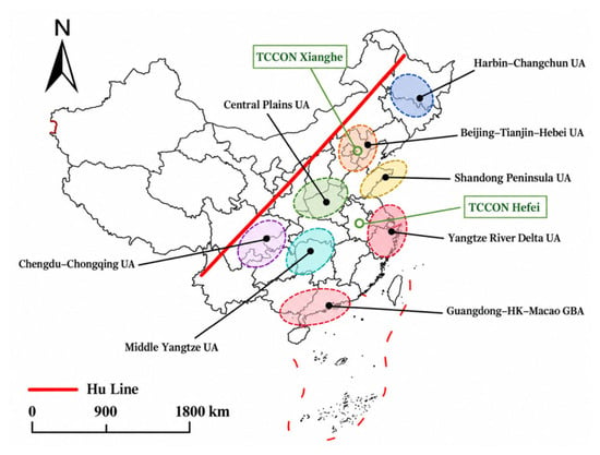
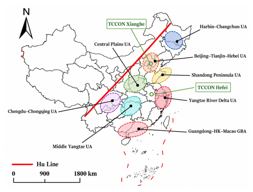
The region east of the Hu Line represents the core concentration area of China’s population, economy, and resources, exhibiting pronounced spatial heterogeneity in its geographical patterns and resource–environmental characteristics. Extending 4318 km along a northeast–southwest axis, this region covers approximately 43.18% of China’s terrestrial area. It is primarily located within the eastern third geomorphic step and the southeastern margin of the second geomorphic step of China, with landscapes dominated by plains and hills, as well as a mosaic distribution of basins and low mountains. The Northeast Plain, North China Plain, Middle and Lower Yangtze Plain, and Sichuan Basin form contiguous agricultural and urban clusters, constituting the largest farming region and urbanized belt in China, with the distribution of major urban agglomerations shown in Figure 1. Meanwhile, mountain ranges such as the Taihang Mountains, Xuefeng Mountains, and Wuyi Mountains intersect with surrounding plains, forming transitional geomorphic zones. These complex landscapes may enhance the complexity of water retention and local atmospheric mixing processes through mountain runoff, fracture infiltration, and terrain-induced ventilation. Under the influence of the East Asian monsoon climate, this region generally receives annual precipitation exceeding 400 mm. The favorable hydrothermal conditions provide suitable environments for agricultural production and ecosystem carbon cycling. In terms of resource distribution, this region contains approximately 80% of China’s cultivated land and 60% of its freshwater resources, while accounting for more than 70% of national energy consumption [16]. As a core region characterized by intensive population concentration, economic activity, and energy consumption in China, the area east of the Hu Line exhibits diverse methane emission sources driven by intensive agricultural activities, dependence on conventional energy resources, and rapid urbanization. Due to limitations in data availability and consistency, Taiwan, Hong Kong, and Macao were not included in the analytical domain of this study.

Figure 1. Geographical setting of the study area east of the Hu Line and locations of TCCON validation sites. Notes: Based on the standard map (Review No. GS(2024)0650) downloaded from the Ministry of Natural Resources Standard Map Service website. No modifications were made to the base map boundaries. The same base map is used in all map figures.

2.2. Satellite Observation Data

The Greenhouse Gases Observing Satellite (GOSAT), developed under the leadership of the Ministry of the Environment of Japan, was successfully launched in 2009. The satellite operates in a sun-synchronous orbit at an altitude of 666 km with a 3-day revisit cycle. The primary scientific payloads onboard GOSAT consist of two complementary sensors: the Fourier Transform Spectrometer (TANSO-FTS), which retrieves greenhouse gas concentrations using observations from the shortwave infrared (SWIR) and thermal infrared (TIR) bands, and the Cloud and Aerosol Imager (TANSO-CAI), which simultaneously acquires cloud distribution and aerosol optical properties to correct radiative interference during the gas retrieval process [17].

Currently, satellite products available for investigating atmospheric column-averaged dry-air mole fractions of methane (XCH₄) mainly include GOSAT, GOSAT-2, and TROPOMI. Although TROPOMI and GOSAT-2 provide higher spatial observation capabilities, their operational periods mainly began around 2018, making them insufficient for independently supporting long-term analyses covering 2010–2024. GOSAT has continuously provided XCH₄ observations since 2009, and its temporal coverage matches the study period considered in this work, making it suitable for constructing a long-term time series based on a consistent data source [18]. Therefore, methane concentration data used in this study were obtained from the official GOSAT Level-3 atmospheric methane concentration product (FTS-SWIR) covering the period 2010–2024 (https://data2.gosat.nies.go.jp/GosatDataArchiveService/usr/download/ProductPage/view, accessed on 28 March 2026). This product is generated from TANSO-FTS observations through rigorous radiometric calibration and gas absorption spectral retrieval algorithms, and is provided as gridded data with a spatial resolution of 2.5° × 2.5°. Spatially averaged methane concentration grid-point data within the study area were extracted using ArcGIS 10.7. The reliability of the satellite-derived observations was evaluated by comparing them with ground-based measurements from TCCON sites.

2.3. Ground-Based TCCON Observations

XCH₄ observations from the TCCON Hefei site (GGG2020.1.R1 version) and the TCCON Xianghe site (GGG2020.1.R0 version) were extracted using Python 3.9 to evaluate the accuracy of GOSAT satellite-derived methane products. TCCON performs solar absorption spectral observations using ground-based Fourier Transform Spectrometers (FTS) and derives column-averaged greenhouse gas concentrations through a standardized retrieval algorithm. Owing to its high measurement accuracy and long-term stability, TCCON has been widely used for the validation and accuracy assessment of satellite-based greenhouse gas products [19]. The temporal resolution of TCCON observations is hourly, and the original measurements are provided in μmol/mol (ppm). To match the temporal scale of the satellite product, the hourly TCCON observations were aggregated into monthly mean XCH₄ concentrations. For each TCCON site, the monthly GOSAT L3 XCH₄ value was extracted from the 2.5° × 2.5° grid cell containing the station coordinates and paired with the corresponding TCCON monthly mean. Thus, the comparison was conducted using spatially collocated satellite grid cells and temporally matched monthly observations. Although this procedure improves spatial and temporal comparability, the GOSAT grid still represents a substantially larger horizontal area than the effective footprint of an individual TCCON station.

2.4. Influence Factors

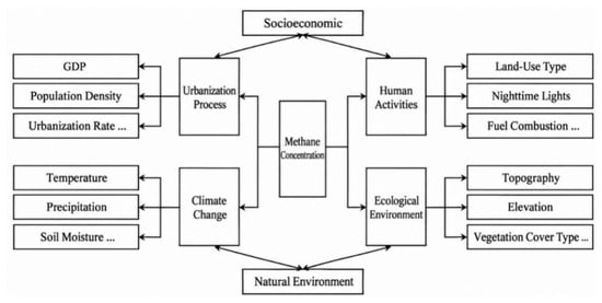
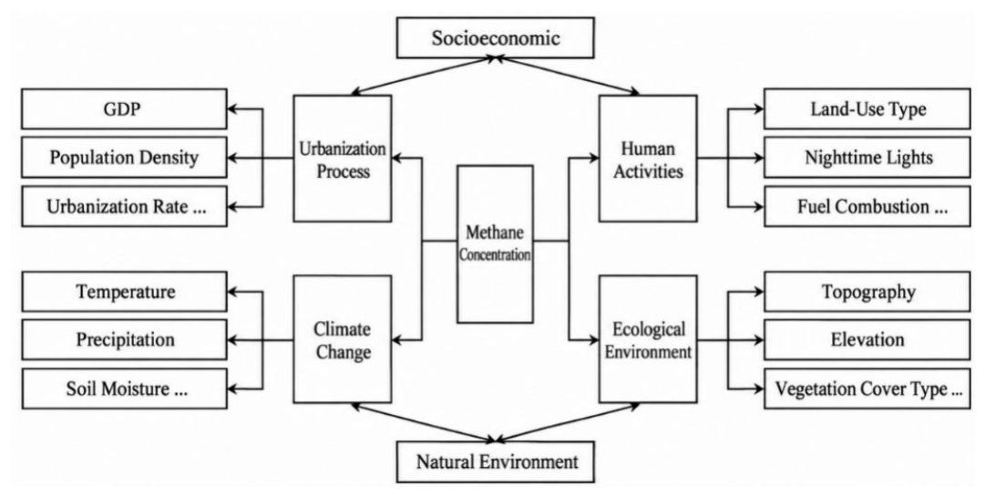
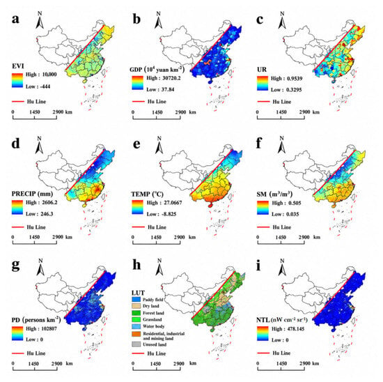
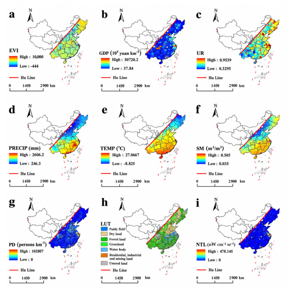
Methane concentrations are jointly influenced by natural environmental conditions and anthropogenic emissions (Figure 2). In this study, data on the Enhanced Vegetation Index (EVI), regional gross domestic product (GDP), population density (PD), land-use type (LUT), and nighttime lights (NTL) were obtained from the Resources and Environmental Science Data Platform. Socioeconomic indicators, including GDP, population density, and nighttime light intensity, were selected to characterize the intensity and spatial distribution of broad anthropogenic activities and urban development [20,21]. The Enhanced Vegetation Index (EVI) is an improved remote sensing index for monitoring vegetation conditions [22], which reduces the limitations of traditional vegetation indices (e.g., NDVI) under atmospheric interference, soil background effects, and high-vegetation-coverage conditions. The original EVI data were stored as scaled integer values and converted using a scale factor of 10⁻⁴. The EVI values shown in Figure 3 represent the original scaled values of the remote sensing product for visualization purposes, whereas the converted EVI values were used in subsequent analyses. Land-use data were obtained from the China Multi-period Land Use and Land Cover Remote Sensing Monitoring Dataset (CNLUCC) [23]. Nighttime light intensity and settlement density data were acquired from the Resources and Environmental Science Data Platform. The GDP dataset was generated through spatial interpolation based on county-level GDP statistics across China and is provided at a spatial resolution of 1 km, with each grid cell representing the total GDP within a 1 km² area, expressed in units of 10⁴ CNY km⁻². Precipitation, temperature, and soil moisture data were obtained from the National Tibetan Plateau Data Center. High-population-density areas are spatially concentrated in urban centers and agglomerations, whereas lower-density areas occupy a larger proportion of the regional land surface. Detailed descriptions of the datasets are provided in Table 1 and Figure 3.

Figure 2. Conceptual framework of potential environmental and socioeconomic controls on CH₄ concentrations.

Figure 3. Spatial distributions of explanatory variables used in this study ((a): EVI, (b): GDP, (c): Urbanization rate, (d): Precipitation, (e): Average temperature, (f): Soil moisture, (g): Population density, (h): Land use type, (i): Night light).

Table 1. Summary of explanatory variables used to characterize potential controls on CH₄ concentrations.

ID	Variable	Abbreviation	Unit	Data Source	Process Category	Proxy Interpretation
X1	Gross domestic product	GDP	104 CNY km−2	Resources and Environmental Science Data Platform	Anthropogenic emission	Proxy for economic activity, energy consumption and anthropogenic emissions
X2	Urbanization rate	UR	-	China Statistical Yearbook	Anthropogenic emission and land change	Proxy for urban development and anthropogenic emission intensity
X3	Land-use type	LUT	-	Resources and Environmental Science Data Platform	Source–sink process	Proxy for surface source–sink characteristics
X4	Population density	PD	persons km−2	Resources and Environmental Science Data Platform	Anthropogenic emission	Proxy for population activity and waste generation
X5	Temperature	TEMP	°C	National Tibetan Plateau Data Center	Source–sink and transport	Proxy for thermal conditions, methane processes and atmospheric transport
X6	Soil moisture	SM	m3 m−3	National Tibetan Plateau Data Center	Source–sink process	Proxy for soil moisture availability and methane oxidation conditions
X7	Enhanced Vegetation Index	EVI	-	Resources and Environmental Science Data Platform	Ecological process	Proxy for vegetation productivity, carbon input and ecosystem conditions
X8	Precipitation	PRECIP	mm	National Tibetan Plateau Data Center	Source–sink and meteorological background	Proxy for hydrothermal conditions and soil moisture availability
X9	Nighttime lights	NTL	nW cm−2 sr−1	Resources and Environmental Science Data Platform	Anthropogenic activity intensity	Proxy for anthropogenic activity intensity and urbanization

Considering the substantial differences in spatial resolution between GOSAT L3 and the explanatory datasets, the native 2.5° × 2.5° GOSAT grid was adopted as the common spatial analysis unit. The finer-resolution explanatory datasets were aggregated to this grid according to variable type, and XCH₄ was not downscaled to finer spatial resolutions. Temperature, precipitation, soil moisture, EVI, population density, and GDP density were aggregated using area-weighted averages based on grid intersections. The urbanization rate was recalculated using population-density-weighted averages within each grid cell. Land-use data were converted into proportional areas of different land-cover categories, and the dominant land-use type within each grid was selected for Geodetector classification analysis. Nighttime light intensity was represented by the mean radiance of valid pixels within each grid cell. All correlation analyses and Geodetector analyses were conducted on the unified 2.5° grid to ensure consistent spatial support between the dependent variable and explanatory factors. Any additional kriging interpolation performed in this study was used only for visualization, not to generate additional samples for the statistical analyses. Due to data availability and the need to maintain consistency and reliability in long-term analyses, correlation calculations and Geodetector analyses were uniformly performed using GOSAT L3 satellite-derived methane data. The year 2023 was selected as the reference year for the cross-sectional factor analysis because of auxiliary-data availability. For the within-grid temporal correlation analysis, complete and consistently matched explanatory-variable datasets were available for 2010, 2015, 2020, and 2023; these four years were therefore used to calculate the temporal correlations.

The atmospheric column-averaged dry-air mole fraction of methane (XCH₄) represents the integrated outcome of surface emissions, atmospheric chemical losses, surface uptake, horizontal transport, and vertical mixing processes. In this study, temperature, precipitation, soil moisture, EVI, and land-use type were selected to characterize hydrothermal conditions and surface ecological backgrounds, whereas GDP, population density, urbanization rate, and nighttime lights were used to represent the intensity of anthropogenic activities. XCH₄ reflects the combined effects of emissions, atmospheric loss, surface uptake, transport, and vertical mixing. In this study, environmental variables characterize hydrothermal and ecological conditions, while GDP, population density, urbanization rate, and nighttime lights represent anthropogenic activity intensity. These indicators are indirect proxies rather than direct measurements of sector-specific methane emissions (Table 1).

2.5. Geodetector Method

Various approaches, including spatial econometric models and geographically weighted regression models, have been developed to investigate the mechanisms underlying geographical phenomena. However, these methods are often insufficient for simultaneously capturing the within-region similarity and between-region heterogeneity of geographical factors. The Geodetector method [24,25,26] is a statistical framework based on the principle of spatial stratified heterogeneity. Unlike conventional statistical models that rely heavily on assumptions of linear relationships and specific data distributions, Geodetector quantifies the explanatory power of individual factors and their interactions, providing an effective tool for analyzing the mechanisms of multidimensional geographical phenomena [24]. Geodetector includes factor detection, which quantifies the spatial stratification of the dependent variable (Y) and evaluates the explanatory power of independent variables (X) by calculating the q-statistic. The q-value ranges from 0 to 1, with larger values indicating stronger explanatory power of X for the spatial differentiation of Y. Interaction detection identifies the synergistic relationship between two factors by comparing the q-values of individual factors with that of their interaction (q(X₁ ∩ X₂)). The corresponding equation is expressed as follows:

$$q=1-{\displaystyle \frac{{\displaystyle {\sum }_{h=1}^L{N}_h{\sigma }_h^2}}{N{\sigma }^2}}=1-{\displaystyle \frac{SSW}{SST}}$$

(1)

$$SSW={\displaystyle \sum _{\mathrm{h}=1}^L{N}_{\mathrm{h}}{{\sigma }^2}_{\mathrm{h}}}$$

(2)

$$SST=N{\sigma }^2$$

(3)

where h represents the stratification of variable Y or factor X; L is the number of strata; N_h denotes the number of units within stratum h; N represents the total number of units in the study area; ${\sigma }_h^2$ is the variance of Y within stratum h; σ² represents the overall variance of Y; SSW is the within-stratum sum of squares; and SST is the total sum of squares for the entire study area. Through stratified variance analysis, Geodetector quantifies the explanatory power of factor X (e.g., land-use type) for the spatial differentiation of variable Y (e.g., methane concentration). The interaction detector in Geodetector is used to evaluate the explanatory power of multiple influencing factors after their interactions. The criteria for identifying different types of interactions are presented in Table 2.

Table 2. Classification criteria for interaction types between two covariates.

Criterion	Interaction Type
q(Xi ∩ Xj) < Min[q(Xi), q(Xj)]	Nonlinear weakening
Min[q(Xi), q(Xj)] < q(Xi ∩ Xj) < Max[q(Xi), q(Xj)]	Univariate weakening
q(Xi) + q(Xj) > q(Xi ∩ Xj) > Max[q(Xi), q(Xj)]	Bivariate enhancement
q(Xi ∩ Xj) = q(Xi) + q(Xj)	Independence
q(Xi ∩ Xj) > q(Xi) + q(Xj)	Nonlinear enhancement

In the Geodetector analysis, a factor-specific discretization strategy was adopted. Continuous variables, including temperature, precipitation, soil moisture, EVI, and nighttime lights, were processed using an optimal-parameter Geodetector approach. The optimal discretization scheme was selected from five classification methods (equal interval, natural breaks, quantile, geometric interval, and standard deviation) combined with 3–8 strata, while ensuring that each stratum contained at least five samples. GDP and population density were classified into five and nine strata, respectively, based on empirical thresholds representing economic density and population agglomeration levels. The dominant land-use type was directly incorporated as a categorical variable in the Geodetector analysis. The urbanization rate was classified using a simulated annealing algorithm that optimized four breakpoints by maximizing the Geodetector q-statistic [27], resulting in five strata, with each stratum containing at least five grid cells.

For continuous variables with optimized discretization parameters [28], statistical significance was evaluated using 9999 selection-adjusted permutation tests. Specifically, after each permutation of XCH₄, the stratification parameter search was repeated to account for the uncertainty introduced by parameter optimization. GDP, population density, and land-use type were evaluated using fixed-stratification permutation tests. Interaction detection was conducted by constructing combined strata based on the final discretization schemes. A total of 9999 permutation tests were performed, and the p-values of 36 interaction pairs were corrected using the Benjamini–Hochberg false discovery rate (FDR) procedure. For interaction pairs involving urbanization rate, the breakpoints of urbanization rate were re-optimized during each permutation to control the potential influence of breakpoint selection on statistical significance.

2.6. Trend Analysis Method

A trend analysis was applied to quantify the long-term variations in XCH₄ concentrations, with the calculation procedure described in Equation (4) [6]. The slope represents the direction and magnitude of temporal changes, where positive and negative slopes indicate increasing and decreasing trends, respectively, while values approaching zero indicate relatively stable concentrations. Based on the slope and significance level (p-value), five trend categories were defined: significant increase (Slope > 0 and p < 0.05), insignificant increase (Slope > 0 and p ≥ 0.05), no obvious change (Slope ≈ 0), insignificant decrease (Slope < 0 and p ≥ 0.05), and significant decrease (Slope < 0 and p < 0.05).

$$slope={\displaystyle \frac{n{\displaystyle {\displaystyle \sum _{i=1}^n}(i{x}_i)}-({\displaystyle {\displaystyle \sum _{i=1}^n}i})({\displaystyle {\displaystyle \sum _{i=1}^n}{x}_i})}{n{\displaystyle \sum _{i=1}^n{i}^2}-{({\displaystyle \sum _{i=1}^{n}i})}^2}}$$

(4)

where slope represents the temporal trend rate of each grid cell over the study period; x_i denotes the XCH₄ concentration value of a given pixel in year i; and n represents the length of the time series.

The Pearson correlation coefficient is a fundamental statistical measure used to quantify the linear relationship between two continuous variables. Its value ranges from −1 to 1, where 1 indicates a perfect positive correlation, −1 indicates a perfect negative correlation, and 0 indicates no linear correlation. It is calculated as the ratio between the covariance of two variables and the product of their standard deviations, reflecting the consistency of their variation trends [6]. The equation is expressed as follows:

$$r={\displaystyle \frac{{\displaystyle {\sum }_{i=1}^n\left(X_i-\overline{X}\right)\left(Y_i-\overline{Y}\right)}}{\sqrt{{\displaystyle {\sum }_{i=1}^n}{\left(X_i-\overline{X}\right)}^2}\sqrt{{\displaystyle {\sum }_{i=1}^n}{\left(Y_i-\overline{Y}\right)}^2}}}$$

(5)

where r represents the Pearson correlation coefficient between satellite-derived XCH₄ observations and influencing factors; X_i and Y_i denote the values of influencing factors and satellite-derived XCH₄ concentrations in the ith grid cell, respectively; $\overline{X}$ and $\overline{Y}$ represent their corresponding mean values. By standardizing covariance with the standard deviations of variables, the equation quantifies the direction (positive or negative) and strength (|r| ∈ [0, 1]) of linear relationships. This approach is particularly suitable for global correlation analysis of normally distributed variables and provides a statistical basis for exploring potential drivers of methane concentrations.

Spearman rank correlation (ρ) was additionally used as a complementary robustness check for the 2023 spatial analysis [29]. It was calculated using the same grid-level observations as the Pearson analysis to examine whether the main associations remained consistent under a rank-based measure. Land-use type was excluded because it is a categorical variable.

Two Pearson correlation procedures were used in this study. First, for the 2023 cross-sectional spatial analysis, the XCH₄ value of each valid grid cell was paired with the corresponding explanatory-variable value, yielding one correlation coefficient for each factor based on 79 spatial observations (n = 79). Second, for the temporal correlations, each grid cell was analyzed separately using four paired annual observations from 2010, 2015, 2020, and 2023 (n = 4 per grid). Repeating this calculation across the 79 grid cells produced the spatial distribution of within-grid temporal correlation coefficients.

3. Results

3.1. Data Validation

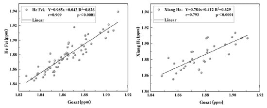
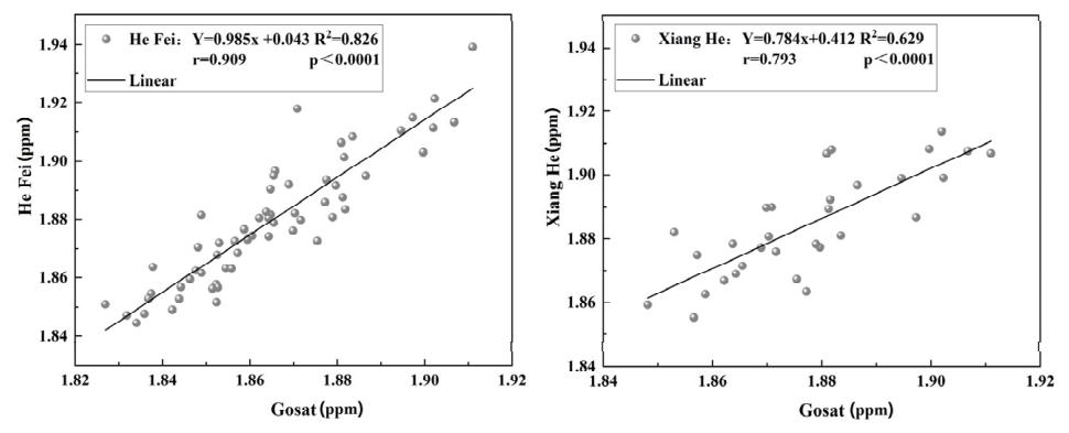
Monthly mean GOSAT XCH₄ concentrations were compared with TCCON observations at the Hefei and Xianghe sites (Figure 4). A total of 91 matched observations were available, comprising 60 samples from Hefei and 31 from Xianghe. The coefficients of determination (R²) were 0.826 and 0.629, and the Pearson correlation coefficients were 0.909 and 0.793, respectively (p < 0.0001). These results indicate positive correspondence between the two datasets at the monthly scale for the matched observations, with closer agreement at Hefei than at Xianghe.

Figure 4. Comparison of monthly GOSAT L3 XCH₄ values from the grid cells containing the Hefei and Xianghe TCCON sites with the corresponding TCCON observations.

3.2. Interannual Variations in XCH₄ Concentrations

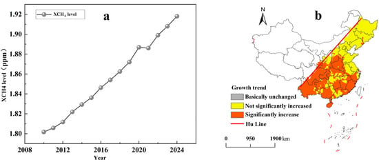
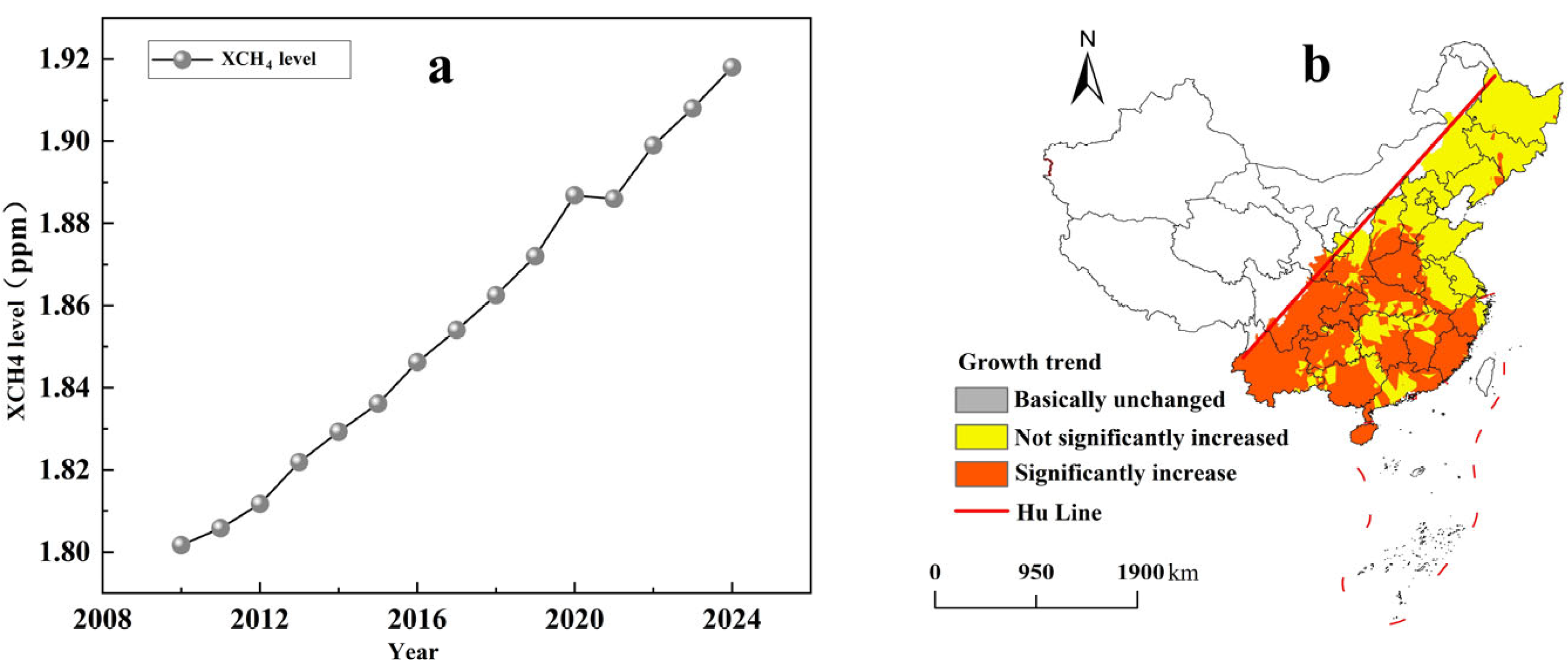
As shown in Figure 5a, annual mean XCH₄ east of the Hu Line increased overall from 1.802 ppm in 2010 to 1.919 ppm in 2024. The cumulative increase was approximately 6.5%, corresponding to a compound annual growth rate of approximately 0.45% and a mean increase rate of approximately 8.36 ppb yr⁻¹. The time series therefore shows an overall upward trend during the study period.

Figure 5. XCH₄ variations east of the Hu Line during 2010–2024: ((a) annual mean concentration; (b) spatial distribution of trend significance).

The spatial significance of this trend varied across the study area (Figure 5b). Significant increases were mainly distributed in southeastern, central, and southwestern China, particularly the middle and lower Yangtze River Plain, the Sichuan Basin, and the eastern Yunnan–Guizhou Plateau. Insignificant increases were mainly observed in the three northeastern provinces, the northern North China Plain, and parts of Shandong, Jiangsu, and Zhejiang. These results distinguish areas with statistically significant increases from those with weaker evidence of an increasing trend.

3.3. Spatial Distribution

3.3.1. Temporal Evolution of XCH₄ Spatial Patterns During 2010–2024

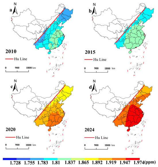
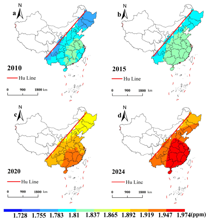
Figure 6 shows the annual mean XCH₄ distributions in 2010, 2015, 2020, and 2024. In 2010, concentrations were generally lower across the study area, with scattered higher-value areas in the middle and lower Yangtze River regions and the Pearl River region. By 2015, higher XCH₄ values had expanded across central and eastern China, particularly in the middle and lower Yangtze River region and parts of the North China Plain, indicating a broader spatial distribution than in 2010. By 2024, relatively high concentrations covered much of the eastern coast and central plains. The maps show a shift toward higher absolute XCH₄ values across much of the study area between 2010 and 2024.

Figure 6. Spatial distribution of annual mean XCH₄ (ppm) east of the Hu Line: ((a) 2010, (b) 2015, (c) 2020, (d) 2024).

3.3.2. Climatological Seasonal Distribution Patterns of XCH₄ from 2010–2024

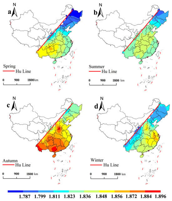
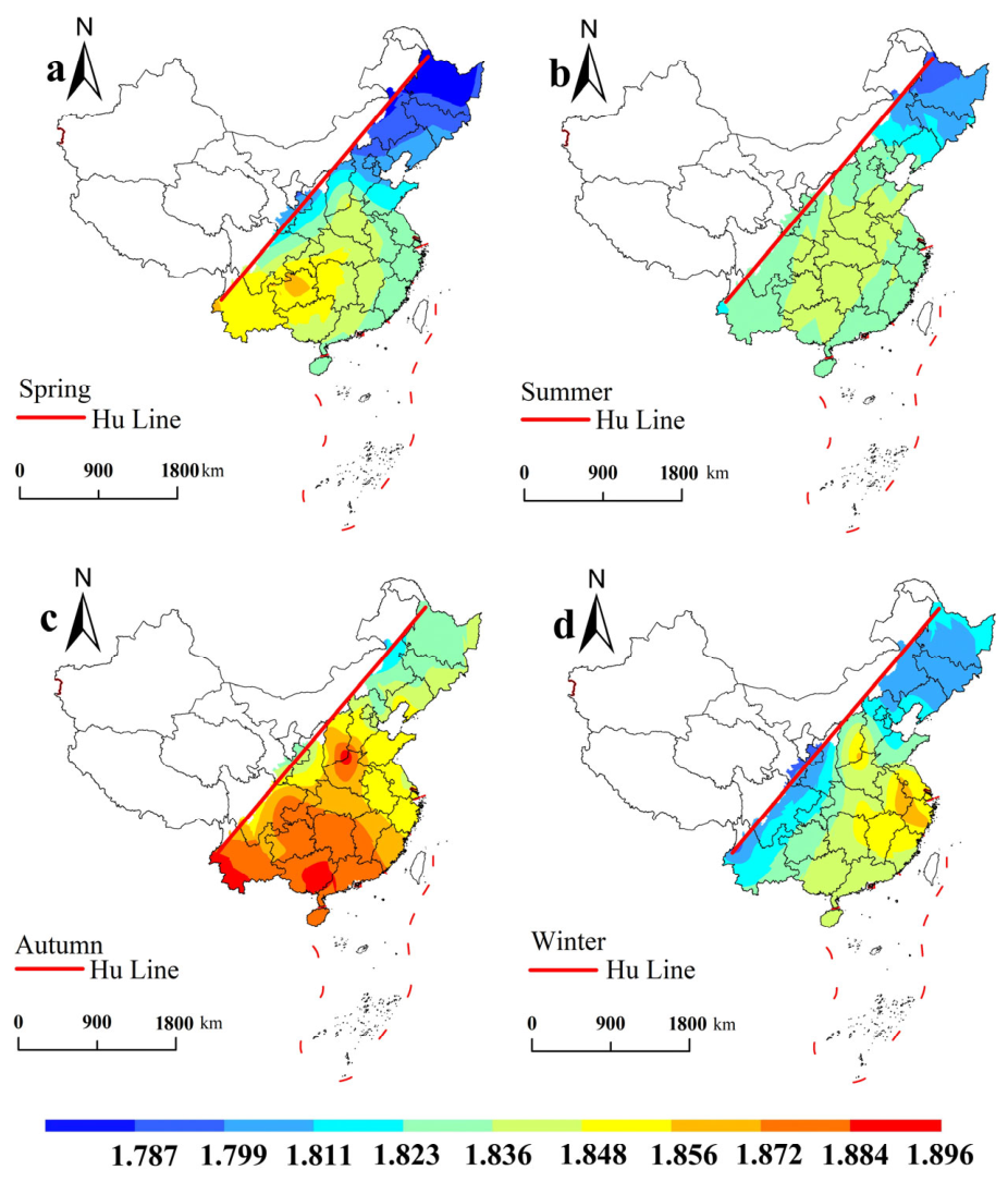
Based on the 2010–2024 multi-year mean values, the climatological seasonal distributions of XCH₄ showed distinct spatial patterns among the four seasons (Figure 7). In spring (March–May), XCH₄ generally exhibited higher concentrations in the south and lower concentrations in the north. In summer (June-August), spatial differences were relatively weaker, and the distribution was more homogeneous than the pronounced south–north pattern observed in spring.

Figure 7. Spatial distribution of seasonal mean XCH₄ (ppm) during 2010–2024: ((a) spring, (b) summer, (c) autumn, (d) winter).

In autumn (September–November), higher XCH₄ concentrations were mainly concentrated in central and southern regions. In winter (January, February, and December), concentrations again exhibited a south–north gradient, with higher values in the south. Overall, the principal seasonal features were the south–north contrasts in spring and winter, relatively weak spatial contrasts in summer, and the concentration of higher values in central and southern regions in autumn.

3.4. Spatial Associations Between XCH₄ and Influencing Factors

3.4.1. Overall Spatial Correlations

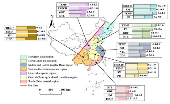
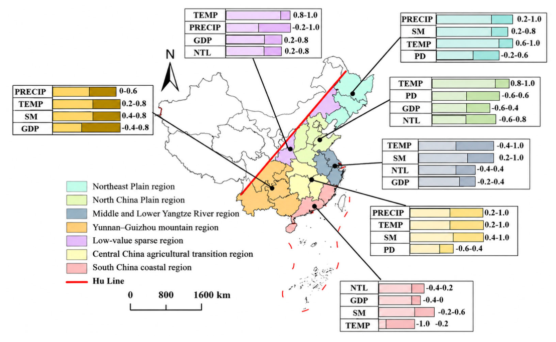
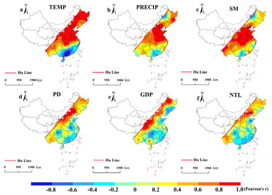
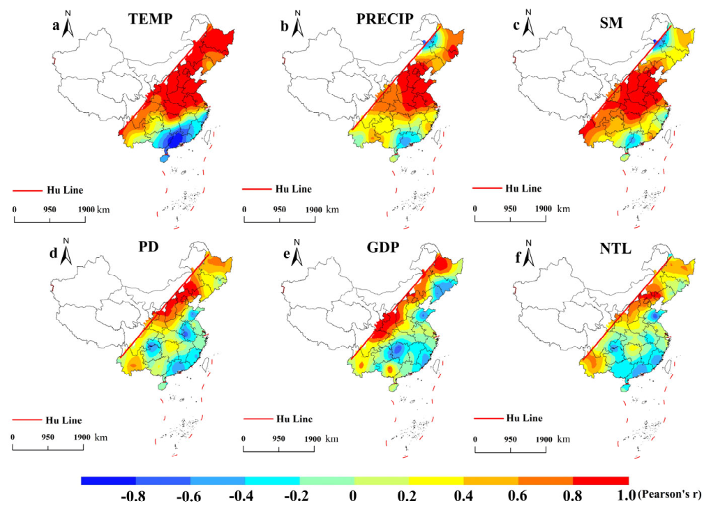
For the representative year 2023, Pearson correlation analysis showed positive associations between XCH₄ and temperature (r = 0.908), precipitation (r = 0.771), soil moisture (r = 0.576), population density (r = 0.546), GDP (r = 0.400), and nighttime lights (r = 0.346). As a complementary robustness check, Spearman rank correlations showed a similar pattern (ρ = 0.884, 0.748, 0.552, 0.487, 0.368, and 0.291, p < 0.05), with temperature and precipitation remaining the two strongest associated factors. The overall consistency between the two measures supports the robustness of the main spatial correlation pattern. Regional summaries and mapped correlation distributions are presented in Figure 8 and Figure 9, respectively.

Figure 8. Representative associated factors and reported correlation-coefficient ranges in different regions. Notes: The dark-colored portions in the figure represent the correlation intervals, and the numbers indicate the correlation magnitudes.

Figure 9. Spatial distribution of correlations between XCH₄ and ((a) temperature, (b) precipitation, (c) soil moisture, (d) population density, (e) GDP, and (f) nighttime lights).

3.4.2. Regional Spatial Association Patterns

In the Northeast Plain region, XCH₄ showed strong positive associations with hydrothermal variables. The correlation ranges of precipitation, temperature, and soil moisture were approximately 0.2 to 1.0, 0.6 to 1.0, and 0.2 to 0.8, respectively. Temperature exhibited the strongest relationship, whereas population density showed a wider range from −0.2 to 0.6, indicating heterogeneous socioeconomic associations.

In the North China Plain, temperature showed the strongest and most consistent correlation with XCH₄, with coefficients ranging from 0.8 to 1.0. In contrast, population density, GDP, and nighttime lights exhibited wider spatial variations, with ranges of −0.6 to 0.6, −0.6 to 0.4, and −0.6 to 0.8, respectively. Compared with hydrothermal factors, socioeconomic indicators showed more heterogeneous spatial patterns.

In the Middle and Lower Yangtze River region, soil moisture showed consistently positive correlations with XCH₄ (0.2 to 1.0), while temperature exhibited substantial spatial variation (−0.4 to 1.0). Nighttime lights and GDP showed relatively weaker and more variable correlations, ranging from −0.4 to 0.4 and −0.2 to 0.4, respectively. This region differed from northern plains by showing stronger variability in temperature and anthropogenic indicators.

In the Central China agricultural transition region, hydrothermal variables showed strong positive relationships with XCH₄. The correlation ranges of precipitation, temperature, and soil moisture were 0.2 to 1.0, 0.2 to 1.0, and 0.4 to 1.0, respectively. Soil moisture exhibited the most stable positive association, whereas population density showed a heterogeneous pattern ranging from −0.6 to 0.4.

In the South China coastal region, XCH₄ exhibited distinct correlation patterns compared with northern and central regions. Temperature showed a strong negative correlation (−1.0 to −0.2), while nighttime lights, GDP, and soil moisture ranged from −0.4 to 0.2, −0.4 to 0, and −0.2 to 0.6, respectively. The opposite temperature relationship highlights the regional differences in XCH₄–climate associations.

In the Yunnan–Guizhou mountain region, precipitation, temperature, soil moisture, and GDP showed correlation ranges of approximately 0.0 to 0.6, 0.2 to 0.8, 0.4 to 0.8, and −0.4 to 0.8, respectively. Compared with plain regions, the correlations were generally moderate, with greater spatial variability among environmental and socioeconomic factors.

In the low-value sparse region, XCH₄ showed strong positive correlations with temperature and socioeconomic indicators. Temperature, precipitation, GDP, and nighttime lights ranged from 0.8 to 1.0, −0.2 to 1.0, 0.2 to 0.8, and 0.2 to 0.8, respectively. Unlike the South China coastal region, this area exhibited consistently positive relationships with temperature and human activity proxies despite its relatively low XCH₄ levels.

Overall, the relationships between XCH₄ and potential explanatory factors exhibited pronounced regional heterogeneity. The Northeast Plain and Central China agricultural transition region showed stronger associations with hydrothermal variables, particularly temperature and soil moisture. The North China Plain was mainly characterized by temperature-related correlations, whereas socioeconomic indicators showed greater spatial variability. The Middle and Lower Yangtze River region, South China coastal region, and low-value sparse region exhibited distinct correlation patterns, including heterogeneous temperature responses and contrasting relationships with anthropogenic indicators. These results highlight the spatially varying roles of hydrothermal conditions, human activities, and regional surface characteristics in shaping XCH₄ distributions.

3.5. Factors Associated with Spatial Heterogeneity in XCH₄

Factor and interaction detection were conducted for 2023 using nine explanatory factors and XCH₄ as the dependent variable. Of the initial 80 satellite grid cells, one boundary grid cell was excluded because of incomplete auxiliary data, leaving 79 grid cells for the analyses.

3.5.1. Factor Stratification and Explanatory Power Assessment

Table 3 summarizes the final stratification schemes. Temperature, precipitation, nighttime lights, and EVI were classified using the quantile method into eight, seven, five, and six strata, respectively. Soil moisture was classified into four strata using the standard-deviation method. GDP and population density were divided into five and nine strata using empirical thresholds [30,31]. The urbanization rate was divided into five strata through simulated-annealing optimization [27]. The four dominant land-use categories were paddy fields, dry croplands, forests, and grasslands.

Table 3. Final stratification schemes and factor-detector results.

Factor	Discretization Method	Number of Strata	q-Statistic	p-Value
Temperature	Quantile	8	0.880	p < 0.05
Precipitation	Quantile	7	0.681	p < 0.05
Population density	Empirical thresholds [30]	9	0.528	p < 0.05
Nighttime lights	Quantile	5	0.518	p < 0.05
Soil moisture	Standard deviation	4	0.401	p < 0.05
EVI	Quantile	6	0.390	p < 0.05
GDP	Empirical thresholds [31]	5	0.348	p < 0.05
Urbanization rate	Simulated annealing optimization [27]	5	0.272	p < 0.05
Land-use type	Original categorical variable	4	0.216	p < 0.05

The single-factor q-statistics followed the order: temperature (0.880) > precipitation (0.681) > population density (0.528) > nighttime lights (0.518) > soil moisture (0.401) > EVI (0.390) > GDP (0.348) > urbanization rate (0.272) > land-use type (0.216). All nine factors were reported as statistically significant (p < 0.05). Temperature and precipitation thus had the greatest explanatory power for the spatial stratification of XCH₄ under the adopted schemes, while population density and nighttime lights ranked highest among the anthropogenic activity proxies.

Temperature-based stratification had the highest single-factor q-statistic (0.880) under the adopted classification scheme. Soil moisture, EVI, and dominant land-use type also differentiated the XCH₄ distribution, although their q-statistics were lower than those of temperature and precipitation.

3.5.2. Interactive Effects Among Explanatory Factors

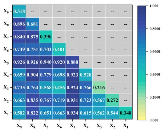
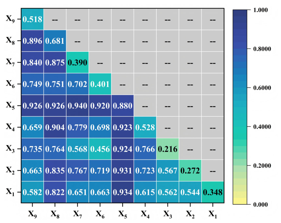
All 36 interaction pairs showed q values exceeding the maximum q value of their corresponding individual factors (Figure 10). Among these pairs, 31 exhibited bivariate enhancement and five exhibited nonlinear enhancement, while no weakening or independence interactions were observed. Following the permutation testing and false discovery rate (FDR) correction procedures described in Section 2.5, all interaction pairs remained statistically significant after Benjamini–Hochberg correction (FDR < 0.05).

Figure 10. Interaction detection results for the explanatory factors.

The largest interaction q-statistic was obtained for temperature ∩ EVI (0.940), followed by temperature ∩ GDP (0.934) and temperature ∩ urbanization rate (0.931). Interactions between temperature and each of the other eight factors ranged from 0.920 to 0.940. Temperature ∩ precipitation and temperature ∩ nighttime lights both had q = 0.926. Precipitation ∩ population density and precipitation ∩ nighttime lights had q-values of 0.904 and 0.896, respectively, and precipitation ∩ EVI had q = 0.875. The ten highest-ranked combinations are listed in Table 4.

Table 4. Top 10 interaction effects among explanatory factors.

Factor Xi	Factor Xj	q(Xi)	q(Xj)	q(Xi ∩ Xj)	Interaction Type
TEMP (X5)	EVI (X7)	0.880	0.390	0.940	Bivariate enhancement
	GDP (X1)		0.348	0.934
	UR (X2)		0.272	0.931
	PRECIP (X8)		0.681	0.926
	NTL (X9)		0.518	0.926
	LUT (X3)		0.216	0.924
	PD (X4)		0.528	0.923
	SM(X6)		0.401	0.920
PRECIP (X8)	PD (X4)	0.681	0.528	0.904
	NTL (X9)		0.518	0.896

These results show that joint stratification by two factors distinguished the XCH₄ distribution more strongly than stratification by either factor alone. Temperature-containing combinations occupied the first eight positions in the interaction ranking.

4. Discussion

XCH₄ integrates source–sink and atmospheric transport processes. The following discussion interprets the observed statistical associations through potential pathways rather than quantitatively attributing source, sink, or transport contributions.

4.1. Spatiotemporal Patterns and Potential Environmental Pathways

The long-term increase in XCH₄ east of the Hu Line is consistent in direction with previous methane studies over China [6,7,9]. In this study, annual mean XCH₄ increased by 117 ppb between 2010 and 2024, corresponding to an endpoint-based mean increase of approximately 8.36 ppb yr⁻¹. This value is close in magnitude to the near-surface methane growth rate of 8.71 ± 0.96 ppb yr⁻¹ reported by Guo et al. [6], providing an external consistency check on the plausibility of the estimated long-term increase. Their numerical similarity supports the general reasonableness of the estimated increase but should not be interpreted as direct quantitative validation.

The expansion of higher-concentration areas may reflect overlapping agricultural, urban, and atmospheric influences. Agricultural land use and rice cultivation provide a possible source context [32,33], while municipal waste disposal provides an additional anthropogenic pathway [34].

Earlier spring warming may advance agricultural activity and microbial processes in southern regions. During summer, greater soil moisture can alter methane production and oxidation in paddy fields, wetlands, and terrestrial soils, while microbial responses depend on anaerobic conditions and substrate availability [35]. Autumn agricultural inputs may sustain methane-producing conditions. Straw incorporation is one pathway through which agricultural management can affect substrate availability in rice paddies [36]. In winter, low temperatures and freeze–thaw processes may restrict or modify microbial activity in northern regions [37,38], whereas agricultural and urban activities continue under the relatively warmer conditions of southern China.

Temperature can affect both methane production and methane oxidation in soils [39], and its net influence depends on water availability, substrate supply, and aeration. Precipitation affects saturation, while drainage and land use determine water retention. Their joint stratification is consistent with combined hydrothermal influences.

EVI characterizes vegetation productivity and carbon input, and vegetation itself responds to climatic conditions [40]. Increased plant productivity, litter input, and root-derived carbon can modify substrate availability, providing a plausible link between vegetation and methane processes [41]. Aerated forest, grassland, and upland soils can consume atmospheric methane [42], whereas wetland vegetation can participate in methane transport from source environments [43]. Methanogenic activity also depends jointly on temperature, substrate availability, and anaerobic conditions [44]. Consequently, a higher EVI does not universally imply a larger methane source. The strong temperature–EVI stratification may therefore reflect complementary vegetation-related and climatic information. The enhanced precipitation-EVI association provides a basis for considering vegetation and water availability together [45]. The interpretation of vegetation-related associations also depends on regional water availability and soil conditions [46,47]. Low-oxygen conditions do not necessarily exclude all methane oxidation [48].

4.2. Anthropogenic Activity and Regional Transport

Population density characterizes population agglomeration, nighttime lights reflect the intensity of illuminated human activities, GDP represents economic activity [49], and the urbanization rate describes urban development. These are proxies rather than direct sector-specific emission measurements. Landfill methane emissions depend on operational and management practices [50,51], while urban wastewater networks contain methane-producing microbial communities [52]. Agricultural sources can occur around urban agglomerations, where rice cultivation and straw incorporation introduce a further source pathway [33,36]. The strong temperature–GDP and temperature–urbanization interactions are consistent with the spatial co-occurrence of relatively warm environments and intensive human activities.

Regional contexts further modify these associations. In the Northeast Plain, wetland and agricultural landscapes provide a setting in which precipitation, soil moisture, and freeze–thaw conditions may be particularly relevant [37]. Rice-management processes offer an additional agricultural pathway [53]. Coastal wetland methane pathways also depend on water level, salinity, vegetation, and substrate availability [54]. Differences in topography and vegetation can also be relevant to ecosystem methane uptake [55].

A 2.5° grid cell can contain local source and uptake signals together with upwind and background contributions. Ventilation may differ among open plains, enclosed basins, coastal areas, and mountain valleys, and urban development can modify regional thermal patterns [56].

4.3. Limitations and Future Perspectives

The spatial resolution of the GOSAT L3 product limits the scale of interpretation. A 2.5° × 2.5° grid cell may contain urban areas, croplands, forests, wetlands, and water bodies, while localized sources such as coal mines, landfills, and oil and gas facilities may be diluted by spatial averaging. The identified patterns therefore characterize regional-scale variability rather than city-scale or individual-source emissions. Kriging was used only for visualization and does not increase the independent spatial information contained in the satellite observations. In addition, representing land use by the dominant category simplifies the coexistence of multiple source and sink environments within a single grid cell.

The TCCON validation is also limited in spatial representativeness. Although the Hefei and Xianghe stations provide independent column-averaged XCH₄ observations and were spatially matched to the corresponding GOSAT grid cells, the two stations represent only two local environments and do not constitute a terrain- or environment-stratified validation network covering the diverse mountainous, basin, transitional, surface, and aerosol conditions within the study area. Therefore, the validation results should be interpreted as site-specific consistency checks rather than as evidence of uniform GOSAT performance across the entire region. Similarly, the annual-scale analysis and coarse spatial resolution cannot resolve short-lived localized changes; therefore, the 2020 XCH₄ pattern should not be directly attributed to temporary emission changes associated with COVID-19 restrictions.

The temporal scopes and sample sizes of the analyses also differ. Long-term XCH₄ trends and seasonal patterns cover 2010–2024, whereas the cross-sectional Pearson, Spearman, and Geodetector analyses use 2023 because of auxiliary-data availability. In contrast, the within-grid temporal correlations shown in Figure 9 are based only on 2010, 2015, 2020, and 2023, for which complete and consistently matched explanatory datasets were available. With only four paired observations per grid, these temporal correlation coefficients are interpreted descriptively and may be sensitive to individual years. The long-term trend analysis also uses a single full-period linear slope based on 15 annual observations per grid. Consequently, temporary reversals, structural breakpoints, and changes in trend rate may not be fully captured. No additional seasonal decomposition or pre-whitening was applied; annual aggregation reduces explicit within-year seasonality but does not guarantee the absence of residual temporal dependence.

The selected explanatory variables are proxies rather than direct observations of methane emission fluxes, ecosystem uptake, atmospheric chemical loss, or transport. Sector-specific methane inventories, atmospheric OH concentrations, wind speed and direction, boundary-layer height, and vertical motions were not included. Accordingly, the present analysis cannot quantitatively separate methane contributions from agriculture, industry, coal mining, or other anthropogenic sectors, nor distinguish the relative effects of local emissions, surface uptake, chemical loss, and regional transport. Pearson and Spearman coefficients describe statistical associations, while Geodetector q-statistics describe spatial stratification and interaction; none of these quantities should be interpreted as sectoral emission fractions or causal contributions. The potential mechanisms discussed in this study therefore require independent process-based evidence.

Future work could integrate sector-resolved inventories for coal mining, oil and gas systems, livestock, rice cultivation, landfills, and wastewater treatment with wetland and soil flux observations, OH-related information, and meteorological datasets such as ERA5 wind fields and boundary-layer height. Finer-resolution satellite observations and additional ground-based validation sites would also improve spatial representativeness. Chemical transport models or atmospheric inversion could then be used to better distinguish source, sink, and transport contributions and to evaluate shorter-term or event-specific methane variability.

5. Conclusions

By integrating a long-term GOSAT L3 satellite record from 2010 to 2024 with ground-based TCCON validation and multi-factor spatial analysis, this study characterized the spatiotemporal variability of XCH₄ east of the Hu Line and examined its associations with environmental and socioeconomic factors. This regional assessment complements previous national-scale studies by treating the region east of the Hu Line as a unified analytical domain. The principal findings are as follows.

(1)

Annual mean XCH₄ increased overall from 1.802 ppm in 2010 to 1.919 ppm in 2024, a cumulative increase of approximately 6.5% and a compound annual growth rate of approximately 0.45%. Significant increases were concentrated in central, southeastern, and parts of southwestern China, including the middle and lower Yangtze River Plain, the Sichuan Basin, and the eastern Yunnan–Guizhou Plateau.

(2)

Higher-concentration areas expanded from scattered distributions toward the eastern coast and central plains. By 2024, prominent higher-value regions included the Yangtze River Delta, Pearl River Delta, North China Plain, and middle and lower Yangtze River region. Seasonal mean patterns showed higher concentrations in the south in spring and winter, weaker spatial contrasts in summer, and a concentration of higher values in central and southern regions in autumn.

(3)

The 2023 cross-sectional correlation analysis across 79 grids showed positive spatial associations between XCH₄ and temperature, precipitation, soil moisture, population density, GDP, and nighttime lights, with temperature and precipitation showing the strongest associations. The supplementary Spearman analysis showed a broadly consistent pattern. In contrast, the within-grid correlations based on four selected years revealed pronounced regional heterogeneity in temporal co-variation, particularly between hydrothermal and socioeconomic factors. Because these within-grid correlations contain only four annual observations, they are interpreted descriptively.

(4)

Temperature (q = 0.880) and precipitation (q = 0.681) had the highest single-factor explanatory power for XCH₄ spatial stratification in 2023. Population density (q = 0.528), nighttime lights (q = 0.518), soil moisture (q = 0.401), EVI (q = 0.390), GDP (q = 0.348), urbanization rate (q = 0.272), and land-use type (q = 0.216) also showed significant explanatory power. All 36 pairwise combinations enhanced spatial explanatory power, with 31 classified as bivariate enhancement and five as nonlinear enhancement. The highest q-values were obtained for temperature ∩ EVI (0.940), temperature ∩ GDP (0.934), and temperature ∩ urbanization rate (0.931).

These findings provide a regional basis for understanding XCH₄ spatial heterogeneity and support further methane monitoring and differentiated mitigation strategies east of the Hu Line.

References

- Zhou, M.Q.; Ni, Q.C.; Wang, J.X.; Cai, Z.N.; Nan, W.D.; Wang, P.C. Retrieval and validation of atmospheric methane column concentration based on infrared hyperspectral remote sensing. Natl. Remote Sens. Bull. 2024, 28, 1968–1985. [Google Scholar]
- Xu, Z.J.; Sun, H.J. Global methane concentrations are rising. Ecol. Econ. 2022, 38, 5–8. [Google Scholar]
- Ministry of Ecology and Environment of the People’s Republic of China. The Fourth Biennial Update Report on Climate Change of the People’s Republic of China; Ministry of Ecology and Environment of the People’s Republic of China: Beijing, China, 2020. [Google Scholar]
- Hu, H.Y. The distribution of population in China, with statistics and maps. Acta Geogr. Sin. 1935, 2, 33–74. [Google Scholar]
- Wang, X.; Fu, X.C.; Xu, W.T.; Yao, L. Characteristics and driving factors of thermal comfort gradient in urban and rural areas of China from 2000 to 2020. Acta Geogr. Sin. 2024, 79, 1318–1336. [Google Scholar] [CrossRef]
- Guo, H.H.; Zhu, W.X.; Zhang, X.Y.; Zhang, H.; Wei, Y.X.; Hou, X.; Xun, N.N. Spatiotemporal distribution characteristics and influencing factors of near-surface methane concentration in China. China Environ. Sci. 2024, 44, 593–601. [Google Scholar]
- Xu, J.H.; Liu, Q.F.; Wang, K.; Wang, Q.L.; Wang, L.; Liu, Y.C.; Li, M.Y. Spatiotemporal variation in near-surface CH4 concentrations in China over the last two decades. Environ. Sci. Pollut. Res. 2021, 28, 47239–47250. [Google Scholar] [CrossRef] [Scilit]
- Xu, Z.C.; Chen, Y.S.; Shan, W.; Deng, C.; Liu, Z.J.; Ji, J. Study on the temporal and spatial distribution of atmospheric methane concentration and the impact of geological emissions in the troposphere in Northeast China during 2003–2022. Clim. Environ. Res. 2025, 30, 77–93. [Google Scholar]
- Peng, Y.Q.; Cai, H.K.; Cai, Z.N. Spatiotemporal characteristics of methane in China during 2003–2018 based on satellite remote sensing monitoring. Remote Sens. Technol. Appl. 2024, 39, 841–849. [Google Scholar]
- Zhang, S.Q. Spatiotemporal Distribution of Atmospheric Methane Concentration in China Based on Ground Monitoring and Satellite Remote Sensing and Its Response to Anthropogenic Emissions. Master’s Thesis, East China Normal University, Shanghai, China, 2022. [Google Scholar]
- Qin, J.; Zhang, X.; Zhang, L.; Cheng, M.; Lu, X. Spatiotemporal variations of XCH4 across China during 2003–2021 based on observations from multiple satellites. Atmosphere 2022, 13, 1362. [Google Scholar] [CrossRef] [Scilit]
- Song, H.; Sheng, M.; Lei, L.; Guo, K.; Zhang, S.; Ji, Z. Spatial and temporal variations of atmospheric CH4 in Monsoon Asia detected by satellite observations of GOSAT and TROPOMI. Remote Sens. 2023, 15, 3389. [Google Scholar] [CrossRef] [Scilit]
- Wang, T.; Wang, Y. XCH4 spatiotemporal variations in a natural-gas-exploiting basin with intensive agriculture activities using multiple remote sensing datasets: Case from Sichuan Basin, China. Remote Sens. 2025, 17, 2695. [Google Scholar] [CrossRef] [Scilit]
- Han, Y.; Wang, C.; Zhang, F.; Li, Q. Research progress and prospects of methods for estimating methane reserves in closed coal mines in China. Processes 2025, 13, 2586. [Google Scholar] [CrossRef] [Scilit]
- Mehrdad, S.M.; Du, K. Satellite-based methane emission monitoring: A review across industries. Remote Sens. 2025, 17, 3674. [Google Scholar] [CrossRef] [Scilit]
- Song, W.F.; Hu, B.B.; Li, H.L.; Yuan, X.S.; Xiao, Z.S.; Hou, X.S. Spatiotemporal pattern evolution and influencing factors of O3 east of the Hu Huanyong Line. Chin. J. Ecol. 2025, 44, 1334–1342. [Google Scholar] [CrossRef]
- National Institute for Environmental Studies. GOSAT Data Products: FTS SWIR Level 3 Products; National Institute for Environmental Studies: Tsukuba, Japan, 2026; Available online: https://www.gosat.nies.go.jp/en/about_5_products.html (accessed on 28 March 2026).
- Qu, Z.; Jacob, D.J.; Shen, L.; Lu, X.; Zhang, Y.; Scarpelli, T.R.; Nesser, H.; Sulprizio, M.P.; Maasakkers, J.D.; Bloom, A.A.; et al. Global distribution of methane emissions: A comparative inverse analysis of observations from the TROPOMI and GOSAT satellite instruments. Atmos. Chem. Phys. 2021, 21, 14159–14175. [Google Scholar] [CrossRef] [Scilit]
- Laughner, J.L.; Toon, G.C.; Mendonca, J.; Petri, C.; Roche, S.; Wunch, D.; Blavier, J.F.; Griffith, D.W.T.; Heikkinen, P.; Keeling, R.F.; et al. The Total Carbon Column Observing Network’s GGG2020 data version. Earth Syst. Sci. Data 2024, 16, 2197–2260. [Google Scholar] [CrossRef] [Scilit]
- Feng, X.H.; Li, Y.; Wang, S.Y.; Yu, E.; Yang, J.Y.; Wu, N.J. Impacts of urban form on carbon emissions under the goal of carbon emission peak and carbon neutrality: A case study of the Yangtze River Economic Belt. Environ. Sci. 2024, 45, 3389–3401. [Google Scholar] [CrossRef] [Scilit]
- Tan, D.; Rao, J.Y. Analysis of influencing factors of urban waterfront space vitality in Shenzhen. J. Geo-Inf. Sci. 2023, 25, 809–822. [Google Scholar] [CrossRef]
- Huete, A.; Didan, K.; Miura, T.; Rodriguez, E.P.; Gao, X.; Ferreira, L.G. Overview of the radiometric and biophysical performance of the MODIS vegetation indices. Remote Sens. Environ. 2002, 83, 195–213. [Google Scholar] [CrossRef] [Scilit]
- Xu, X.L.; Liu, J.Y.; Zhang, S.W. Multi-Period Land Use and Land Cover Remote Sensing Monitoring Dataset of China (CNLUCC); Institute of Geographic Sciences and Natural Resources Research; Chinese Academy of Sciences: Beijing, China, 2018. [Google Scholar] [CrossRef]
- Wang, J.F.; Li, X.H.; Christakos, G.; Liao, Y.L.; Zhang, T.; Gu, X.; Zheng, X.Y. Geographical detectors-based health risk assessment and its application in the neural tube defects study of the Heshun region, China. Int. J. Geogr. Inf. Sci. 2010, 24, 107–127. [Google Scholar] [CrossRef] [Scilit]
- Wang, J.F.; Zhang, T.L.; Fu, B.J. A measure of spatial stratified heterogeneity. Ecol. Indic. 2016, 67, 250–256. [Google Scholar] [CrossRef] [Scilit]
- Wang, J.F.; Ge, Y.; Li, L.F.; Meng, B.; Wu, J.L.; Bai, Y.C.; Du, S.H.; Liao, Y.L.; Hu, M.G.; Xu, C.D. Geographic spatiotemporal data analysis methods. Acta Geogr. Sin. 2014, 69, 1326–1345. [Google Scholar] [CrossRef]
- Karacan, I.; Senvar, O.; Bulkan, S. A novel parallel simulated annealing methodology to solve the no-wait flow shop scheduling problem with earliness and tardiness objectives. Processes 2023, 11, 454. [Google Scholar] [CrossRef] [Scilit]
- Song, Y.; Wang, J.; Ge, Y.; Xu, C. An optimal parameters-based geographical detector model enhances geographic characteristics of explanatory variables for spatial heterogeneity analysis: Cases with different types of spatial data. GISci. Remote Sens. 2020, 57, 593–610. [Google Scholar] [CrossRef] [Scilit]
- Godwin, P.; Tian, S.; Duvert, C.; Wurm, P.; Riwu Kaho, N.; Edwards, A. Detecting groundwater dependence and woody vegetation restoration with NDVI and moisture trend analyses in an Indonesian karst savanna. Front. Remote Sens. 2024, 5, 1280712. [Google Scholar] [CrossRef] [Scilit]
- Yang, Q.; Li, L.; Wang, Y.D.; Wang, X.Y.; Lu, Y.C. Spatial pattern of China’s population distribution and its evolution characteristics from 1935 to 2010. Geogr. Res. 2016, 35, 1547–1560. [Google Scholar]
- Jing, B.; Li, T.S.; Wen, B.Q.; Cheng, W.H. Study on the population-economic spatial pattern and its influencing mechanism in the Qinba Mountain area based on terrain factors. Sci. Geogr. Sin. 2020, 40, 793–803. [Google Scholar] [CrossRef]
- Xu, W.B.; Rao, L.Y. Impacts of land use and climate change on ecosystem services in agro-pastoral ecotone. Environ. Sci. 2023, 44, 5114–5124. [Google Scholar] [CrossRef] [Scilit]
- Li, S.Q.; Hua, E.S.; Chen, M.P. Evolution of spatial pattern and technical mitigation potential of methane emissions from rice in China. China Environ. Sci. 2025, 45, 1218–1230. [Google Scholar] [CrossRef]
- Zhan, J.F.; Wang, S.S. Prediction and assessment of methane source carbon emissions from municipal solid waste landfills in China. Environ. Sci. Technol. 2022, 45, 147–155. [Google Scholar] [CrossRef]
- Liu, S.J.; Liu, C.P.; Fang, L.P.; Chen, G.H.; Li, F.B. Analysis of arsenic methylation characteristics and mechanisms of butyrate-dependent methanogenic microbial communities in paddy soils. Ecol. Environ. Sci. 2024, 33, 1580–1589. [Google Scholar]
- Yan, X.; Yagi, K.; Akiyama, H.; Akimoto, H. Statistical analysis of the major variables controlling methane emission from rice fields. Glob. Change Biol. 2005, 11, 1131–1141. [Google Scholar] [CrossRef]
- Zhang, C.F.; Sheng, L.X.; Gong, C.; He, C.G.; Zhang, J. Effects of freeze-thaw processes on soil carbon emissions and soil microorganisms in wetlands of Northeast China. Chin. J. Ecol. 2018, 37, 304–311. [Google Scholar] [CrossRef]
- Yang, T.; Duan, Y.T.; Liu, Y.Q.; Sun, F.H.; Liu, X.S.; Zheng, C.L.; Wang, Z. Effects of freeze-thaw cycles on soil bacterial community structure and metabolic function. J. Anhui Agric. Sci. 2024, 52, 62–66. [Google Scholar] [CrossRef]
- Ding, W.X.; Cai, Z.C. Effects of temperature on methane production and oxidation in soils. Chin. J. Appl. Ecol. 2003, 14, 604–608. [Google Scholar]
- Yang, M.X.; Li, J.; Tong, X.J.; Yu, P.Y.; Wang, Y.T.; Shi, Q.; Wang, Y. Response of EVI to climate factors in forest vegetation in China from 2001 to 2020. Acta Ecol. Sin. 2024, 44, 10850–10863. [Google Scholar]
- Girkin, N.T.; Siegenthaler, A.; Lopez, O.; Stott, A.; Ostle, N.; Gauci, V.; Sjögersten, S. Plant root carbon inputs drive methane production in tropical peatlands. Sci. Rep. 2025, 15, 3244. [Google Scholar] [CrossRef] [Scilit]
- Cai, Y.F.; Jia, Z.J. Research progress of atmospheric methane-oxidizing bacteria in soils. Acta Microbiol. Sin. 2014, 54, 841–853. [Google Scholar] [CrossRef]
- Vroom, R.J.E.; van den Berg, M.; Pangala, S.R.; van der Scheer, O.E.; Sorrell, B.K. Physiological processes affecting methane transport by wetland vegetation: A review. Aquat. Bot. 2022, 182, 103547. [Google Scholar] [CrossRef] [Scilit]
- Conrad, R. Complexity of temperature dependence in methanogenic microbial environments. Front. Microbiol. 2023, 14, 1232946. [Google Scholar] [CrossRef] [Scilit]
- Brooks, P.D.; Troch, P.A.; Durcik, M.; Gallo, E.; Schlegel, M. Quantifying regional scale ecosystem response to changes in precipitation: Not all rain is created equal. Water Resour. Res. 2011, 47, W00J08. [Google Scholar] [CrossRef] [Scilit]
- Chen, S.; Zhao, W.W.; Han, Y. Spatiotemporal variation characteristics and influencing factors of vegetation precipitation use efficiency in arid and semi-arid regions of China. Acta Ecol. Sin. 2023, 43, 10295–10307. [Google Scholar] [CrossRef]
- Zhou, L.; Du, M.; Yang, X.N.; Zhang, A.J.; Rong, G.H.; Li, B.W. Responses of soil physicochemical properties to different vegetation structures in gully areas of the Loess Plateau. For. Ecol. Sci. 2025, 40, 182–188. [Google Scholar] [CrossRef]
- Ma, R.C.; Wei, X.M.; He, R. Research progress on hypoxia tolerance mechanisms and community structure of aerobic methanotrophs in oxygen-limited environments. Chin. J. Appl. Ecol. 2017, 28, 2047–2054. [Google Scholar] [CrossRef]
- Xu, X.L. Chinese GDP Spatial Distribution Kilometer Grid Dataset; Resource and Environmental Science Data Registration and Publishing System: Beijing, China, 2017. [Google Scholar] [CrossRef]
- Scharff, H.; Soon, H.Y.; Taremwa, S.R.; Zegers, D.; Dick, B.; Villas Bôas Zanon, T.; Shamrock, J. The impact of landfill management approaches on methane emissions. Waste Manag. Res. 2024, 42, 1052–1064. [Google Scholar] [CrossRef] [Scilit]
- Xu, H.Y. Control of greenhouse gas emissions and development prospects of landfills in China. Environ. Sanit. Eng. 2024, 32, 13–18. [Google Scholar]
- Sun, G.X.; Jin, P.K.; Song, J.N.; Wang, X.B.; Yang, K.Y. Distribution characteristics of methanogens in urban sewer networks. Environ. Sci. 2016, 37, 2252–2258. [Google Scholar] [CrossRef]
- Feng, Y.F.; Xia, L.; Yin, K.Y. Research on methane emission in paddy fields and countermeasures: A case study of Liaoning Province. Agric. Technol. 2025, 45, 103–106. [Google Scholar] [CrossRef]
- Wang, J.; Yuan, J.J.; Liu, D.Y.; Xiang, J.; Ding, W.X.; Jiang, X.J. Research progress on methane production pathways and methanogens in coastal wetlands. Chin. J. Appl. Ecol. 2016, 27, 993–1001. [Google Scholar] [CrossRef]
- Li, Y. Effects of Topography and Vegetation Cover on Respiration and Methane Uptake in Alpine Meadow Ecosystems. Master’s Thesis, University of Chinese Academy of Sciences, Beijing, China, 2020. [Google Scholar]
- Xu, L.L.; Wang, J.; Zhou, W.Q. Influence of urban agglomeration development on the evolution of regional heat island spatial patterns. Acta Ecol. Sin. 2024, 44, 11035–11048. [Google Scholar] [CrossRef]
Disclaimer/Publisher’s Note: The statements, opinions and data contained in all publications are solely those of the individual author(s) and contributor(s) and not of MDPI and/or the editor(s). MDPI and/or the editor(s) disclaim responsibility for any injury to people or property resulting from any ideas, methods, instructions or products referred to in the content. |
© 2026 by the authors. Licensee MDPI, Basel, Switzerland. This article is an open access article distributed under the terms and conditions of the Creative Commons Attribution (CC BY) license.