A Hybrid CNN–iTransformer Framework with Physics-Informed Regularization for Accurate MOSFET RUL Estimation

Abstract

Accurate forecasting of MOSFET on-state resistance drift can support remaining useful life (RUL) estimation under thermal overstress. Existing methods seldom combine local degradation patterns, long-range feature interactions, and a failure-mode-specific prior in one forecasting framework. We propose a CNN–iTransformer model that uses on-state resistance drift as its health indicator and includes a finite-difference sensitivity constraint. On the four test records reported in this study, the average mean absolute error (MAE), root mean square error (RMSE), and relative error (RE) were 2.996 × 10⁻⁴ Ω, 3.988 × 10⁻⁴ Ω, and 3.110 × 10⁻³, respectively. For Test 37, the predicted RUL was 850 sampling steps versus 843 observed steps, producing a seven-step absolute error. These results concern within-record forecasting on one accelerated-aging dataset; generalization to unseen devices remains to be established.

1. Introduction

Metal-oxide-semiconductor field-effect transistors (MOSFETs) are key components of modern power conversion systems [1,2], including electric vehicle inverters, grid-connected photovoltaic converters, and industrial motor drives [3]. As these high-power applications expand, MOSFET reliability becomes increasingly important for system safety, energy-conversion efficiency, and maintenance planning [4,5,6]. During prolonged operation under harsh conditions, including high voltage, large load current, and cyclic junction-temperature variations, MOSFETs undergo irreversible degradation [7]. Among the candidate precursor parameters, the on-state resistance is particularly relevant to die-attach degradation induced by thermal and power cycling. Its applicability is, therefore, failure-mode-dependent and should not be generalized to gate-oxide-related degradation without additional electrical indicators [8]. The resistance’s deviation from its initial value has been widely validated in the literature [9,10,11] as a sensitive, non-invasive, and quantifiable health indicator (HI) [12]. Its evolution exhibits a strong correlation with accumulated device wear, making the accurate modeling and forecasting of $\Delta R_{ds\left(on\right)}$ the cornerstone of remaining useful life (RUL) estimation for power electronics [13]. Notably, RUL estimation is the core of prognostics and health management (PHM) [14], which further highlights the significance of $\Delta R_{ds\left(on\right)}$ in device reliability analysis.

Existing MOSFET lifetime prediction methods can be categorized into three main paradigms, each with inherent advantages and non-negligible limitations. Physics-based models rely on fundamental degradation mechanisms, such as hot-carrier injection (HCI) [15], time-dependent dielectric breakdown (TDDB) [16], and negative bias temperature instability (NBTI) [17]. These mechanisms mainly concern die-intrinsic gate-oxide degradation; they are not the degradation modes modeled in the present study, which focuses on die-attach degradation under thermal-overstress conditions. These models excel in interpretability and extrapolation under known stress conditions, as they directly map physical processes to device degradation [18]. However, their practical application is constrained by strict prerequisites: they require precise knowledge of material properties, defect evolution kinetics, and real-time operating profiles [19]. This makes them difficult to generalize across different device generations or adapt to real-world mission profiles with complex load transients [20,21], ultimately limiting their scalability in industrial scenarios.

In response to the above challenges, data-driven machine learning techniques have gained increasing attention in recent years [22,23], including artificial-neural-network-based prognosis of power MOSFET resistance degradation trends [24]. Their key advantage lies in learning complex degradation patterns directly from operational or experimental data, without relying on explicit physical assumptions. Early data-driven efforts focused on traditional machine learning algorithms, such as support vector regression (SVR) [25] and Gaussian process regression (GPR) [26]. While these methods achieved reasonable performance for short-term prediction, they struggled to capture long-term temporal dependencies and handle high-dimensional input features—two critical requirements for MOSFET RUL prediction.

With the advancement of deep learning, recurrent neural networks (RNNs), such as long short-term memory (LSTM) and gated recurrent units (GRUs), were introduced to MOSFET RUL prediction. These models effectively address the vanishing gradient problem of traditional RNNs, enabling more accurate modeling of sequential degradation dynamics [27]. Baharani et al. [28] introduced a deep learning framework employing stacked LSTM networks to assess the collective reliability of MOSFET converter arrays, experimental validation across five distinct devices demonstrates a low average prediction error of 8.9%, significantly outperforming established classical methods. Ibrahim et al. [29] proposed a novel data-driven framework that employs LSTM and GRU networks to translate dominant failure precursor data into long-term lifetime projections for power MOSFETs. The developed prognostic model was shown to yield accurate and actionable predictions, directly addressing real-world reliability challenges by providing an effective estimation tool. However, they still face two key limitations: poor performance in modeling very long prediction horizons and lack of parallel computing capability, which restricts their efficiency for large-scale datasets. More recently, transformer-based models have emerged as a powerful alternative, leveraging parallelization and global attention mechanisms to capture long-range dependencies [30,31] and have been applied to SiC MOSFET lifetime prediction across working conditions [32]. Gao et al. [9] proposed a robust predictive framework, which was constructed by merging the global search prowess of a genetic algorithm for hyperparameter tuning with the comprehensive attention scope of a Transformer. The proposed model substantially outperforms conventional particle filter benchmarks, achieving a significantly lower average absolute percentage error. This corresponds to an improvement by a factor of three to five in predictive accuracy. Luo et al. [33] proposed a hybrid prediction model, autoformer-regularized extreme learning machine, resulting in significantly improved prediction accuracy. Despite this progress, pure transformer models often overlook local temporal patterns and are prone to overfitting on small-scale degradation datasets-a common issue in MOSFET aging experiments, where obtaining large amounts of data is costly and time-consuming.

Physical consistency has been extensively studied in battery prognostics and health management. Hybrid physics-informed neural networks have combined reduced-order electrochemical models with neural correction terms for battery modeling and prognosis [34], physics-informed LSTM frameworks have coupled calendar- and cycle-aging models with operational data for online RUL prediction [35], and PINN-based schemes have fused semi-empirical degradation dynamics with data-driven representations [36]. More directly, monotonic relationships between battery health factors and state of health have been converted into physical constraints within the learning objective [37]. These studies establish that physics-informed learning and monotonic regularization are well-developed ideas in battery health management.

The corresponding problem in power MOSFET prognostics is less developed. Among the representative studies considered here, existing approaches primarily rely on feedforward neural networks [24], LSTM/GRU models [29], transformer-based forecasting [9,32,33], or deep reinforcement learning [38]. These methods have advanced device lifetime prediction, but the explicit integration of a failure-mode-specific monotonic prior with a hybrid local–global forecasting architecture has received limited attention. For die-attach-dominated thermal-overstress aging, the relevant physical quantity is the irreversible increase in ΔR_ds(on), rather than battery capacity fade; the constraint must, therefore, be linked to the package-level failure mechanism, the selected health indicator, the forecast trajectory, and the end-of-life threshold.

To address this device-specific gap, this work combines a one-dimensional CNN and an iTransformer to forecast on-state resistance drift under thermal overstress. The CNN extracts local patterns from the univariate health-indicator sequence, while the iTransformer models interactions among learned latent channels. A finite-difference sensitivity constraint expresses the prior that a higher historical degradation level should not lower the average forecast. The use of a CNN, iTransformer, or monotonic prior is not individually new; the study examines their combination for MOSFET prognosis. The constraint acts on sensitivity to input perturbation and does not guarantee that every predicted future step is non-decreasing.

2. Proposed Model

The proposed framework for MOSFET RUL prediction is built upon a hybrid deep learning architecture that integrates a CNN with an inverted Transformer, enhanced by a physics-informed regularization term. The input to the model is a standardized univariate sequence of the LOWESS-smoothed on-state resistance drift, denoted by $\tilde{s}(t)$. For an observation window of length L, the input is expressed as $X_t={[\tilde{s}(t-L+1),\dots ,\tilde{s}(t)]}^{\mathrm{T}}$. The CNN converts this input into a multichannel latent feature sequence, which is subsequently processed by the iTransformer to predict the next H values of the resistance-drift trajectory. After inverse standardization, the model output represents the predicted on-state resistance drift in ohms and is used to estimate the time to the predefined failure threshold. The following section outlines the three core components of the proposed methodology, with particular focus on the iTransformer architecture and the physics-informed constraint.

2.1. CNN Feature Extractor

In the proposed framework, a CNN [39] is integrated at the input stage. It extracts local temporal features from the preprocessed degradation signal and suppresses measurement noise along with spurious transients. Let the input sequence be denoted as follows:

$$x={[x_1,x_2,\dots ,x_L]}^T\in R^L,$$

(1)

where $x_t$ represents the on-resistance drift at time step t, and L is the length of the observation window.

The CNN processes x through stacked convolutional operations, each applying learnable filters to capture short-range dependencies. The transformation in a generic layer can be expressed as

$$z=\sigma (w\ast x+b),$$

(2)

where w and b are the learnable kernel and bias, ∗ denotes the 1D convolution operator, and σ(⋅) is a non-linear activation function. This operation enables the network to adaptively highlight degradation-relevant patterns-such as monotonic trends or acceleration points while attenuating high-frequency artifacts.

The CNN preserves the temporal structure of the input and transforms the univariate degradation sequence, $X_t$, into a latent feature sequence, $F_{\mathrm{CNN}}$. Each output channel represents a learned numerical descriptor of the local degradation pattern, such as the local slope, curvature, or short-term variation. These channels are latent features and do not correspond one to one to separately measured physical quantities. The resulting feature sequence is subsequently passed to the iTransformer to model longer-range dependencies and generate the future on-state resistance-drift trajectory.

2.2. iTransformer Module

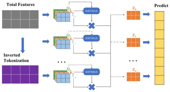
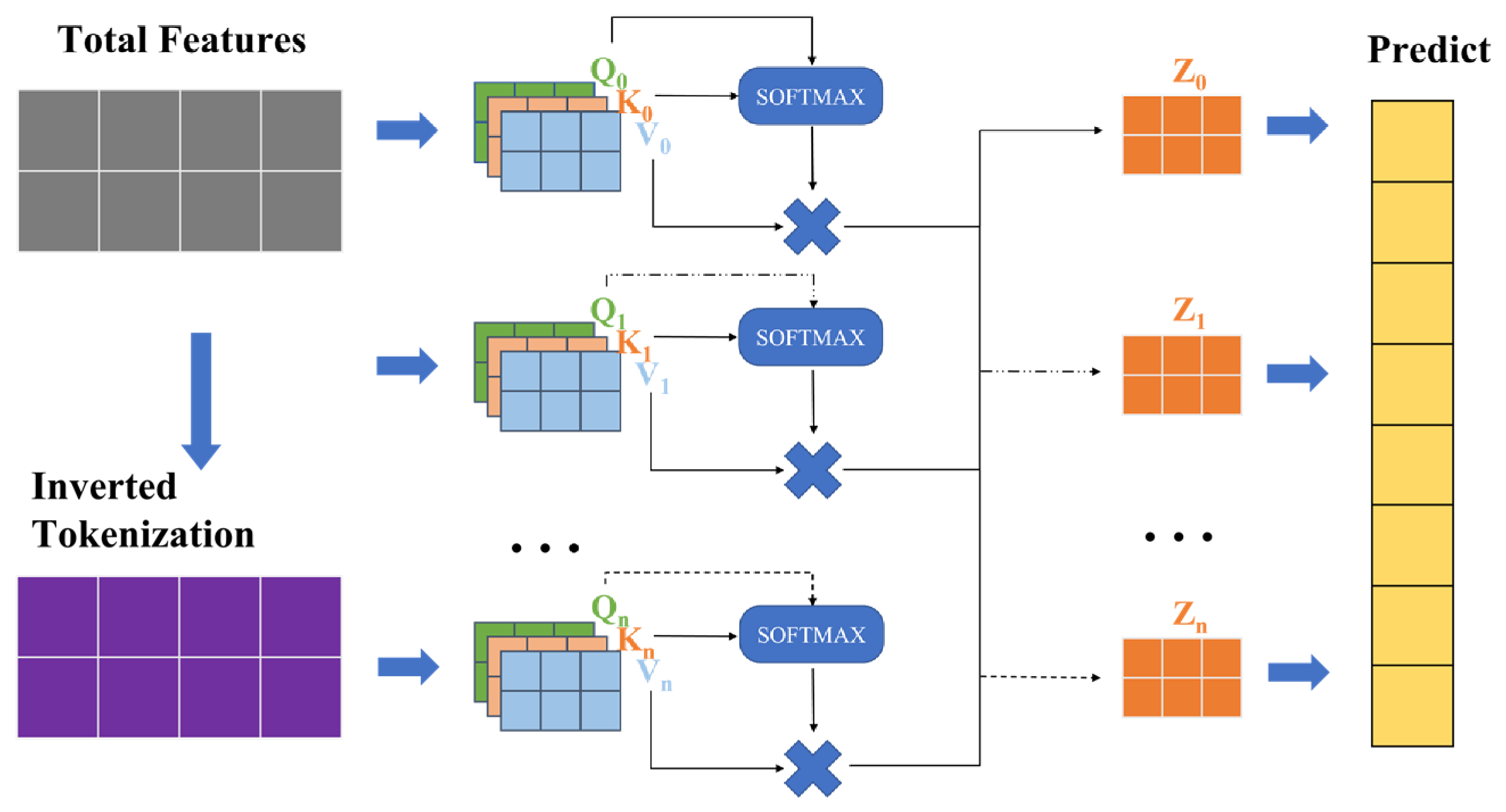
The iTransformer architecture rethinks the role of Transformer components in multivariate time-series forecasting by inverting the conventional tokenization and attention axes [40]. The structure of the iTransformer is shown in Figure 1. In standard Transformers, every time step is represented as a token, and self-attention operates over the temporal dimension to model long-range temporal dependencies. However, this design may conflate distinct physical variables into a single fused representation per timestamp, leading to ambiguous attention maps and reduced forecasting accuracy, especially when the variates exhibit asynchronous dynamics or delayed relationships.

Figure 1. Diagram of the proposed iTransformer architecture. Arrows indicate information flow. Q, K, and V denote query, key, and value matrices, respectively, and Z denotes an attention output. Multiplication signs denote matrix multiplication; ellipses in-dicate repeated attention branches.

To address this problem, iTransformer proposes a simple yet effective inversion: each variate is embedded as a separate token, and the sequence of its historical observations forms the feature vector of that token. Formally, given a multivariate time-series input,

$$X={\left[x_1,x_2,\dots ,x_T\right]}^T\in R^{T\times N},$$

(3)

where T is the lookback window length and N is the number of variates, iTransformer transposes the input to obtain

$$\tilde{X}=X^T\in R^{N\times T},$$

(4)

where each row, ${\tilde{x}}_i$, now represents the full temporal history of the i-th variate and is treated as a variate token.

These N tokens are then passed through a standard Transformer encoder. The self-attention mechanism operates across the N variable tokens to learn multivariate correlations explicitly. Consequently, the model captures the dynamic interactions among the different CNN latent feature channels. Simultaneously, the feed-forward network (FFN) is applied independently to each token, operating along the temporal dimension, T. This allows the FFN to model complex, non-linear temporal dynamics within each individual variate, effectively functioning as a per-series temporal learner.

Mathematically, after the optional linear projection and positional encoding, the Transformer encoder computes

$$Attention\left(Q,K,V\right)=softmax({\displaystyle \frac{Q{K}^T}{\sqrt{d}}})V,$$

(5)

where $Q,K,V$ are derived from the N variate tokens, and d is the embedding dimension. The subsequent FFN applies a two-layer MLP to each row of the attention output. By processing each feature vector independently, it captures intra-variate temporal patterns.

For forecasting, the final representation of each variate token is projected to the prediction horizon H via a learnable linear head:

$$\widehat{Y}=W_{out}\cdot Encoder{(\tilde{X})}^T+b_{out}\in R^{T\times H},$$

(6)

and the output is reshaped to yield the forecast, $\widehat{Y}$.

This inverted design decouples inter-variate correlation modeling from intra-variate temporal modeling, aligning the Transformer’s strengths with the inherent structure of multivariate time series. This design retains standard Transformer components while separating inter-variate correlation modeling from intra-variate temporal modeling. It also supports extended look-back windows and provides more interpretable attention maps.

2.3. Physics-Informed Constraint

To encourage consistency with the expected long-term degradation trend, a finite-difference sensitivity term is included in the training objective. It provides a limited prior for the thermal-overstress records studied here.

In the thermal-overstress dataset considered in this study, the increase in R_ds(on) is mainly associated with irreversible die-attach degradation induced by repeated power cycling. Accordingly, the predicted lifetime refers to package-level degradation rather than die-intrinsic gate-oxide degradation. As the die-attach degradation accumulates, the long-term $\Delta R_{ds\left(on\right)}(t)$ trend is expected to be non-decreasing. Denoting the degradation state at time t as s(t), we have the following physical constraint:

$${\displaystyle \frac{d\Delta R_{ds\left(on\right)}}{ds}}\ge 0.$$

(7)

This prior regularizes the model response to an increase in the historical degradation level.

The model maps a historical resistance-drift sequence to a future prediction. Here the constraint concerns the forecast response to an upward perturbation of the input sequence, rather than the temporal differences between successive predicted future values.

$${\displaystyle \frac{\partial {\widehat{y}}_{\tau }}{\partial x_t}}\ge 0,\hspace{1em}\forall t\in \{1,\dots ,L\}, \tau \in \{1,\dots ,H\}.$$

(8)

However, directly computing this Jacobian is computationally expensive for long sequences and high-dimensional outputs.

We use a scalarized measure of forecast sensitivity to a uniform perturbation of the historical input. This directional finite difference is defined using the perturbed inputs:

$$x_{enc}^{+}=x_{enc}+\epsilon 1,\hspace{1em}{x}_{enc}^{-}=x_{enc}-\epsilon 1,$$

(9)

where ε is a small constant. The numerical derivative of the model’s prediction is then approximated via the central difference formula:

$${\displaystyle \frac{d\widehat{y}}{d{x}_{enc}}}\approx {\displaystyle \frac{f_{\theta }(x_{enc}^{+},\cdot )-f_{\theta }(x_{enc}^{-},\cdot )}{2\epsilon }}\in {ℝ}^{H\times 1},$$

(10)

This quantity represents the average forecast sensitivity to an increase in the historical degradation level. It is not the time derivative of the future degradation trajectory.

To enforce the non-negativity of this derivative, we introduce a hinge loss that penalizes only violations of the physical prior:

$${\mathcal{L}}_{\mathrm{phy}}={\displaystyle \frac{1}{H}}{\displaystyle \sum _{\tau =1}^H}\max \left(0,-{\left[{\displaystyle \frac{d\widehat{y}}{d{x}_{enc}}}\right]}_{\tau }\right),$$

(11)

The penalty is zero when the finite-difference sensitivity is non-negative. This does not by itself enforce a non-decreasing forecast across time.

The total training loss combines this physics-informed term with the standard forecasting loss:

$$\mathcal{L}={\displaystyle \frac{1}{H}}{\displaystyle \sum _{\tau =1}^H}{\left({\widehat{y}}_{\tau }-y_{\tau }\right)}^2+{\lambda }_{\mathrm{phy}}{\mathcal{L}}_{\mathrm{phy}},$$

(12)

where ${\lambda }_{phy}$ is a tunable hyperparameter that balances data fidelity and physical consistency.

The perturbed forward passes retain gradient tracking, allowing the physics-informed penalty to contribute to parameter updates. The input perturbation magnitude was ε = 0.001 in standardized input units, and the physics-informed loss weight was λ_phy = 1. These settings were fixed for the reported experiments; their sensitivity was not assessed.

The constraint provides a limited prior for the studied die-attach-dominated aging process. It does not constitute a complete physical degradation model or a hard guarantee of temporal monotonicity.

3. Experimental Workflow

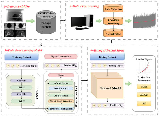
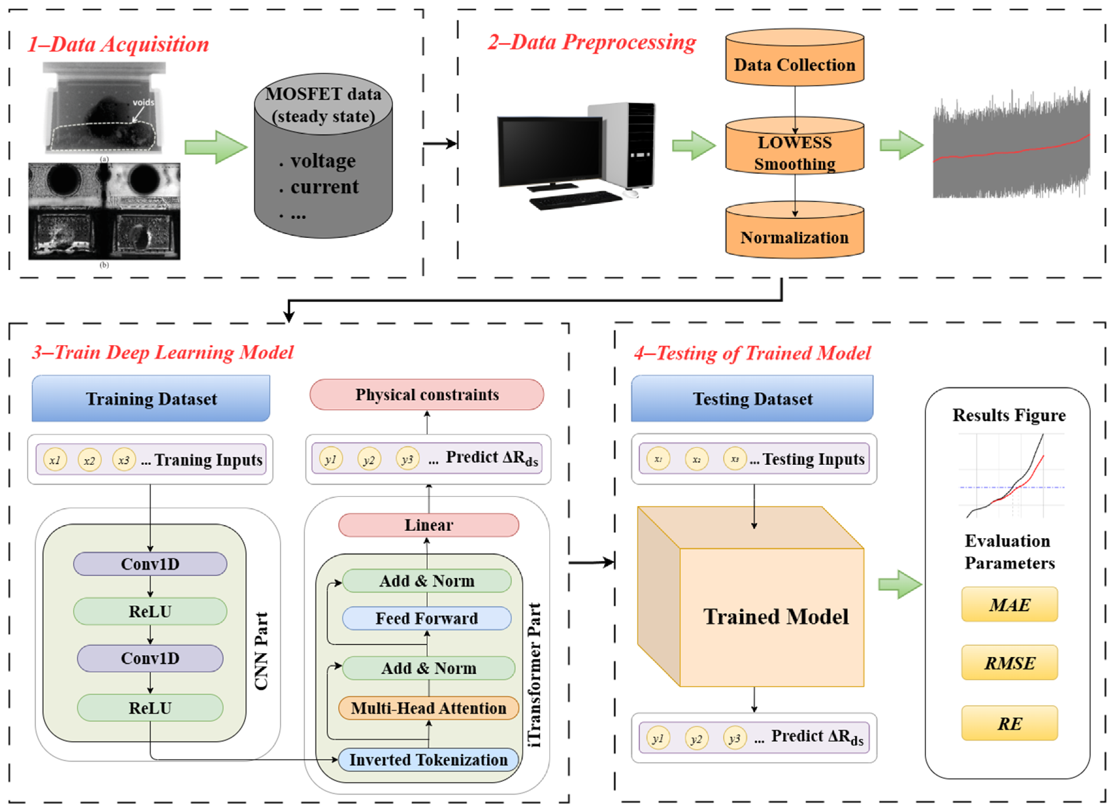
The overall workflow of the proposed MOSFET RUL prediction framework is illustrated in Figure 2 and consists of four sequential steps: (1) The drain-source voltage, drain current, flange temperature, and package temperature are extracted from the original aging records. The on-state resistance is calculated from the drain-source voltage and drain current, and its signed drift relative to the initial baseline is subsequently smoothed using LOWESS. (2) The smoothed resistance-drift sequence is standardized using statistics calculated from the training partition. (3) The standardized univariate sequence is supplied to the CNN–iTransformer model to predict its future evolution. (4) The predicted values are transformed back to the original resistance unit and compared with the 0.05 Ω failure threshold for RUL estimation. Each step is detailed below.

Figure 2. CNN–iTransformer prediction framework. (a) X-ray microscopy and (b) scanning acoustic microscopy images of a degraded device, repro-duced from. Black and green arrows indicate workflow and data flow. Gray and red curves illustrate raw and smoothed data; colors distinguish processing blocks. The acquisition block lists recorded voltage, current, and temperature channels; only resistance drift is supplied to the prog-nostic model.

3.1. Dataset Construction

In this study, we utilize the publicly available MOSFET Thermal Overstress Aging dataset provided by NASA’s Prognostics Center of Excellence (PCoE) [41]. In this study, the on-state resistance drift is employed as a failure-mode-specific health indicator for die-attach-dominated degradation under thermal-overstress conditions. The NASA aging experiments used here were conducted through repeated power cycling, under which degradation of the die-attach layer increases the junction-to-case thermal resistance and produces a measurable increase in R_ds(on). In addition, R_ds(on) can be obtained non-invasively from the in situ drain-source voltage and drain current measurements available in the dataset. Therefore, its selection is based on both its physical relationship with the dominant failure mechanism and its availability in the experimental records.

The original accelerated-aging experiments were conducted on IRF520Npbf power MOSFETs in TO-220 packages. Thermal cycling was induced by repeated power cycling without an external heat sink, while the device case temperature was measured and used as the control variable. The gate was driven by an approximately 15 V square-wave signal at 1 kHz with a duty cycle of 40%. The drain-source terminals were biased at 4 V DC, and a 0.2-Ω resistive load was used. The drain-source voltage and drain current were measured in situ, and R_ds(on) was calculated from their ratio during the on state. The original study describes the device temperature as varying from room temperature to a high-temperature setting; however, a fixed numerical ambient temperature and the complete numerical temperature-cycle profile were not reported. Therefore, the applicability of the present model is limited to degradation conditions represented by this public thermal-overstress dataset.

The device-run records in the public archive differ in signal-channel completeness, continuity, recording duration, and acquisition end point; consequently, not every nominal run supports a directly comparable RUL label under a common failure definition. Before model training, the records were, therefore, screened using model-independent data-suitability criteria: (1) sufficiently complete and synchronized drain-source voltage and drain-current measurements to reconstruct a continuous on-state-resistance trajectory; (2) adequate sequence length for the common historical and forecast windowing protocol without substantial missing intervals or acquisition discontinuities; and (3) after baseline correction and LOWESS preprocessing, a physically plausible degradation evolution covering the threshold-relevant region of the adopted ΔR_ds(on) = 0.05 Ω EOL definition, so that a consistent RUL target could be assigned. Based on these criteria, Test_26, Test_36, Test_37, and Test_38 were retained for model evaluation. No record was selected according to forecasting accuracy, and each retained record corresponds to a distinct device-run experiment rather than a segment extracted from a common record.

The analysis is restricted to the four retained records. Because record-level exclusions are not quantified here, possible selection bias should be considered when interpreting the reported accuracy.

3.2. Denoising and Normalization

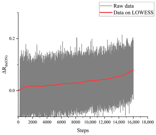
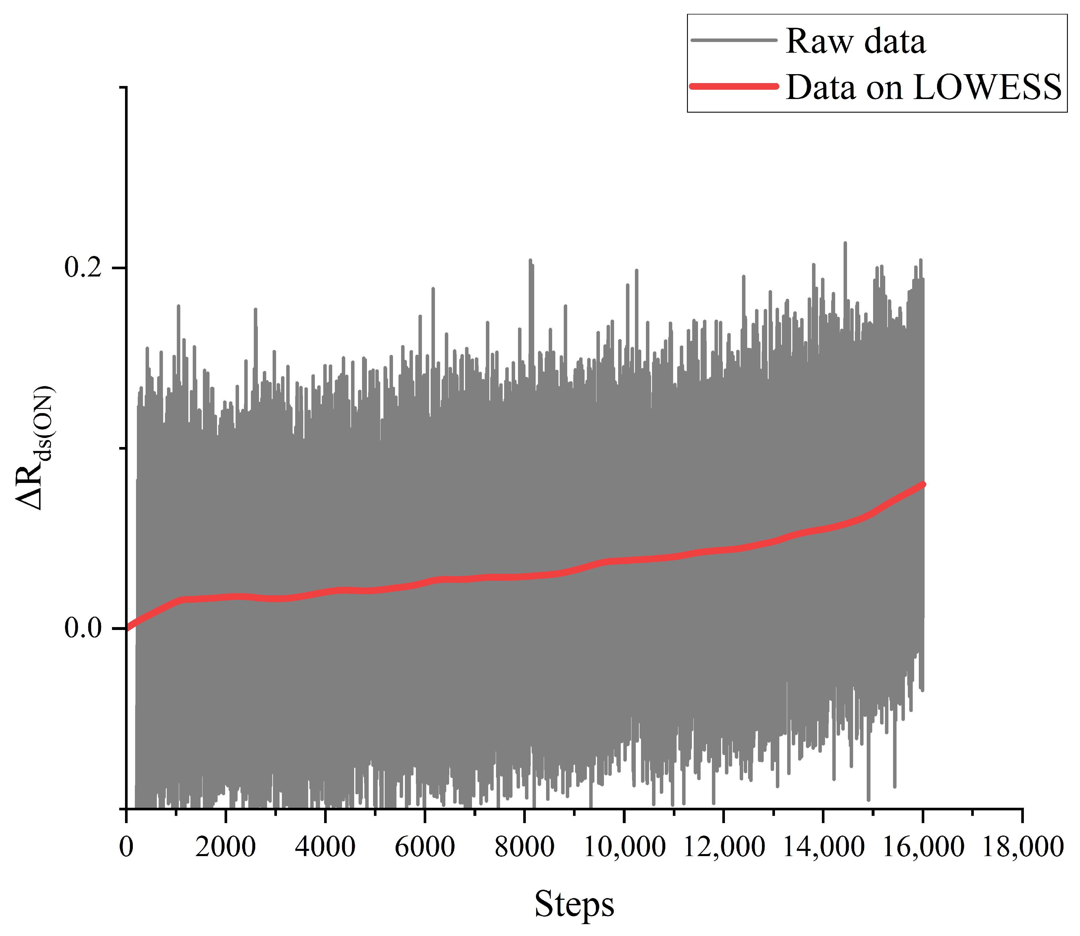
Raw measurements of the on-resistance, $R_{ds\left(on\right)}$, from accelerated-aging tests are often contaminated by high-frequency noise arising from sensor limitations, electromagnetic interference, or transient thermal effects. Such artifacts can obscure the intrinsic degradation trend and mislead data-driven models into capturing spurious short-term variations rather than the underlying physical aging process. To address this, we apply Locally Weighted Scatterplot Smoothing (LOWESS)—a robust non-parametric regression technique—to each device’s time series. Given an observation, $x_j=\Delta R_{ds\left(on\right)}\left(t_j\right)$, the smoothed value, ${\tilde{x}}_j$, is computed as

$${\tilde{x}}_j={\displaystyle \sum _{k=1}^N}{w}_{jk}{x}_k,$$

(13)

where the weights, $w_{jk}$, are derived from a tricube kernel that emphasizes temporally proximate points, with a smoothing bandwidth that controls the local neighborhood. The schematic diagram after filtering is shown in Figure 3. LOWESS effectively suppresses measurement noise while preserving the monotonic and gradually accelerating nature of MOSFET degradation, which is essential for reliable long-term forecasting.

Figure 3. Comparison of the filtered data trajectories. The gray curve shows raw data, and the red curve shows the LOWESS-smoothed trajectory.

Following the denoising, the entire dataset undergoes global standardization using statistics computed solely from the training partition:

$${\widehat{x}}_t={\displaystyle \frac{{\overline{x}}_t-{\mu }_{\mathrm{train}}}{{\sigma }_{\mathrm{train}}}},$$

(14)

where ${\mu }_{train}$ and ${\sigma }_{train}$ denote the mean and standard deviation of the training data. This normalization ensures that input features are centered and scaled consistently across all devices, thereby improving numerical stability during optimization and supporting consistent scaling across the selected records. By jointly mitigating noise and aligning data distributions, this preprocessing stage yields a clean, standardized degradation signal that serves as a robust foundation for physics-informed deep learning.

3.3. Model Training

The CNN consists of two one-dimensional convolutional layers with channel sizes 1, 64, and 64, a kernel size of 3, a stride of 1, and padding of 1. A ReLU activation follows each convolutional layer. The iTransformer uses an embedding dimension of 64, 4 attention heads, 2 encoder layers, a feed-forward dimension of 128, and a dropout rate of 0.1. The observation-window length is L = 32 samples, and the prediction horizon is H = 10 samples.

The core learning component of the framework is trained to perform direct multi-step forecasting of the normalized degradation signal. Given a historical segment of $x_{1:L}={[{\widehat{x}}_1,{\widehat{x}}_2,\dots ,{\widehat{x}}_L]}^T$, extracted from the preprocessed time series of a device, the model learns a mapping of $f_{\theta }:R^L\to R^H$ that predicts the next H values of the sequence:

$${\widehat{y}}_{L+1:L+H}=f_{\theta }\left(x_{1:L}\right),$$

(15)

where θ denotes the learnable parameters. The training dataset is constructed by sliding a window of length L + H across all available device trajectories, yielding input-target pairs $\left(x_{1:L}, y_{L+1:L+H}\right)$. The model is optimized to minimize the mean squared error (MSE) between predicted and ground-truth future values:

$${\mathcal{L}}_{\mathrm{MSE}}={\displaystyle \frac{1}{H}}{\displaystyle \sum _{\tau =1}^H}{\left({\widehat{y}}_{L+\tau }-y_{L+\tau }\right)}^2,$$

(16)

this formulation enables the network to capture both short-term fluctuations and long-term drift patterns in a single forward pass, supporting efficient and coherent multi-step prediction without recursive error accumulation. Training uses the Adam optimizer with an initial learning rate of 0.001 and a batch size of 32, together with learning-rate decay. Early stopping uses a patience of 10 epochs, and the checkpoint with the lowest validation loss is retained. Validation-based selection can reduce overfitting, but it does not establish performance on devices absent from model development. The present study does not claim an exhaustive hyperparameter search.

3.4. RUL Estimation

At inference time, the trained model takes the most recent L-step window of normalized $\Delta R_{ds\left(on\right)}$ as input and predicts the next τ values. Under the online rolling-evaluation protocol, non-overlapping τ-step forecast blocks are updated using the most recent observed history and concatenated to form the predicted test trajectory. RUL is then estimated as the number of sampling steps from the prediction origin to the first predicted resistance-drift value that reaches the EOL threshold. The monotonicity constraint promotes a physically plausible degradation trajectory during this threshold-based inference.

For RUL evaluation, let $t_{i,0}$ denote the first forecasted sample of test record i, and let $y_i(t)$ and ${\widehat{y}}_i(t)$ denote the measured and predicted on-state resistance drift, respectively. With the EOL threshold ${\delta }_{\mathrm{EOL}}$ = 0.05 Ω, the measured and predicted failure indices are defined by the first threshold-crossing samples of the two trajectories. The saved test trajectories are concatenations of non-overlapping forecasts that are updated after each forecast block, consistent with the online rolling-evaluation protocol used for the trajectory metrics.

$$t_{i,\mathrm{EOL}}=\min \left\{t\ge t_{i,0}\mid y_i(t)\ge {\delta }_{\mathrm{EOL}}\right\},{\widehat{t}}_{i,\mathrm{EOL}}=\min \left\{t\ge t_{i,0}\mid {\widehat{y}}_i(t)\ge {\delta }_{\mathrm{EOL}}\right\},$$

(17)

$${\mathrm{RUL}}_i=t_{i,\mathrm{EOL}}-t_{i,0},{\widehat{\mathrm{RUL}}}_i={\widehat{t}}_{i,\mathrm{EOL}}-t_{i,0}.$$

(18)

4. Experimental Results and Analysis

To validate the effectiveness of the proposed CNN–iTransformer framework with physics-informed constraints, we conducted comprehensive experiments on the public MOSFET Thermal Overstress Aging dataset from NASA. This section presents a detailed analysis of the experimental setup, evaluation metrics, and performance results, highlighting both the quantitative accuracy and physical consistency.

4.1. Introduction of Experimental Data

For each of the four selected device records, the first 70% of the sequence was used for model development and the final 30% for testing in chronological order, as in the original evaluation. The original manuscript does not specify a separate validation allocation within the first 70%. The test portions, therefore, represent later observations from records already used in model development. This is within-record temporal forecasting, not a strict test on completely unseen devices.

The experimental study utilizes the publicly available MOSFET thermal overstress aging dataset from NASA’s Prognostics Center of Excellence (PCoE). This dataset records the degradation behavior of commercial IRF520Npbf power MOSFETs under accelerated-aging conditions. Devices are subjected to repeated thermal–electrical stress cycles. The repeated thermal–electrical cycling primarily induces progressive degradation of the die-attach layer. Consequently, the on-state drain-source resistance exhibits a measurable and monotonic increase. This resistance shift serves as a well-established health indicator in power electronics.

The model input is the signed on-state resistance drift relative to an initial baseline, derived from on-state voltage and current and then smoothed. It is the only measured feature supplied to the prognostic model. The CNN channels are learned latent descriptors, not independent measurements of threshold voltage, gate leakage current, junction temperature, or switching behavior.

A critical aspect of the experimental setup is the EOL definition. Following established practice in semiconductor reliability studies, a device is considered to have failed when the health indicator reaches or exceeds 0.05 Ω. This threshold corresponds to a physically meaningful degradation level. Such degradation significantly impacts switching performance and thermal management in practical applications. All predictive evaluations in this study are anchored to this failure criterion. This ensures consistency in RUL estimation across devices.

4.2. Evaluation Metrics

The accuracy of predicted on-resistance drift is evaluated using three standard regression metrics: mean absolute error (MAE), root mean squared error (RMSE), and relative error (RE). For the i-th time step in the forecast window, let ${\widehat{y}}_i$ and $y_i$ denote the predicted and ground-truth values, respectively. These metrics are formally defined as:

$$\mathrm{MAE}={\displaystyle \frac{1}{n}}{\displaystyle \sum _{i=1}^n}\left|\Delta {\widehat{R}}_{\mathrm{ds}\left(\mathrm{on}\right)}^{\left(i\right)}-\Delta R_{\mathrm{ds}\left(\mathrm{on}\right)}^{\left(i\right)}\right|,$$

(19)

$$\mathrm{RMSE}=\sqrt{{\displaystyle \frac{1}{n}}{\displaystyle \sum _{i=1}^n}{\left(\Delta {\widehat{R}}_{\mathrm{ds}\left(\mathrm{on}\right)}^{\left(i\right)}-\Delta R_{\mathrm{ds}\left(\mathrm{on}\right)}^{\left(i\right)}\right)}^2},$$

(20)

$$\mathrm{RE}={\displaystyle \frac{1}{n}}{\displaystyle \sum _{i=1}^n}{\displaystyle \frac{\left|\Delta {\widehat{R}}_{\mathrm{ds}\left(\mathrm{on}\right)}^{\left(i\right)}-\Delta R_{\mathrm{ds}\left(\mathrm{on}\right)}^{\left(i\right)}\right|}{\Delta R_{\mathrm{ds}\left(\mathrm{on}\right)}^{\left(i\right)}}}.$$

(21)

MAE reports the mean absolute error in the original unit of $\Delta R_{\mathrm{ds}\left(\mathrm{on}\right)}$. RMSE emphasizes large-magnitude discrepancies, serving as an indicator of prediction robustness. RE normalizes error by the true degradation level, which is particularly informative during early aging stages when the health indicator exhibits low amplitude. All metrics are calculated using the inverse-transformed resistance-drift trajectories. MAE and RMSE are expressed in ohms, whereas RE is dimensionless. These metrics evaluate the accuracy of the predicted degradation trajectory and do not represent errors in the CNN latent features or temperature measurements.

In addition to the trajectory-level MAE, RMSE, and RE, direct RUL performance is evaluated using the absolute RUL error (AE_RUL), relative RUL error (RE_RUL), and RUL prediction precision (P_RUL):

$${\mathrm{AE}}_{\mathrm{RUL},i}=\left|{\widehat{\mathrm{RUL}}}_i-{\mathrm{RUL}}_i\right|,$$

(22)

$${\mathrm{RE}}_{\mathrm{RUL},i}={\displaystyle \frac{\left|{\widehat{\mathrm{RUL}}}_i-{\mathrm{RUL}}_i\right|}{{\mathrm{RUL}}_i}}\times 100\%,$$

(23)

$${\mathrm{P}}_{\mathrm{RUL},i}=\left(1-{\displaystyle \frac{\left|{\widehat{\mathrm{RUL}}}_i-{\mathrm{RUL}}_i\right|}{{\mathrm{RUL}}_i}}\right)\times 100\%.$$

(24)

The direct RUL comparison is limited to Test 37, using the same prediction origin, end-of-life threshold, and evaluation protocol for the six listed methods.

In addition to the preceding accuracy metrics, residual analysis was used to characterize the deterministic forecast error. For device record i, let T_i denote the set of valid test indices and let N_i = |T_i| denote the corresponding number of samples. The pointwise residual, mean residual, and residual standard deviation are defined as follows:

$$e_i(t)=y_i(t)-{\widehat{y}}_i(t), t\in {\mathcal{T}}_i,$$

(25)

$${\overline{e}}_i={\displaystyle \frac{1}{N_i}}{\displaystyle \sum _{t\in {\mathcal{T}}_i}{e}_i}(t),$$

(26)

$$s_{e,i}=\sqrt{{\displaystyle \frac{1}{N_i-1}}{\displaystyle \sum _{t\in {\mathcal{T}}_i}{\left(e_i(t)-{\overline{e}}_i\right)}^2}}.$$

(27)

A positive residual indicates underestimation of the degradation magnitude. Because consecutive samples originate from rolling time-series forecasts, the residual statistics are used descriptively and the sampling points are not treated as independent replicates.

4.3. Experimental Results and Discussion

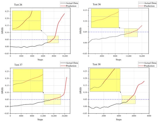
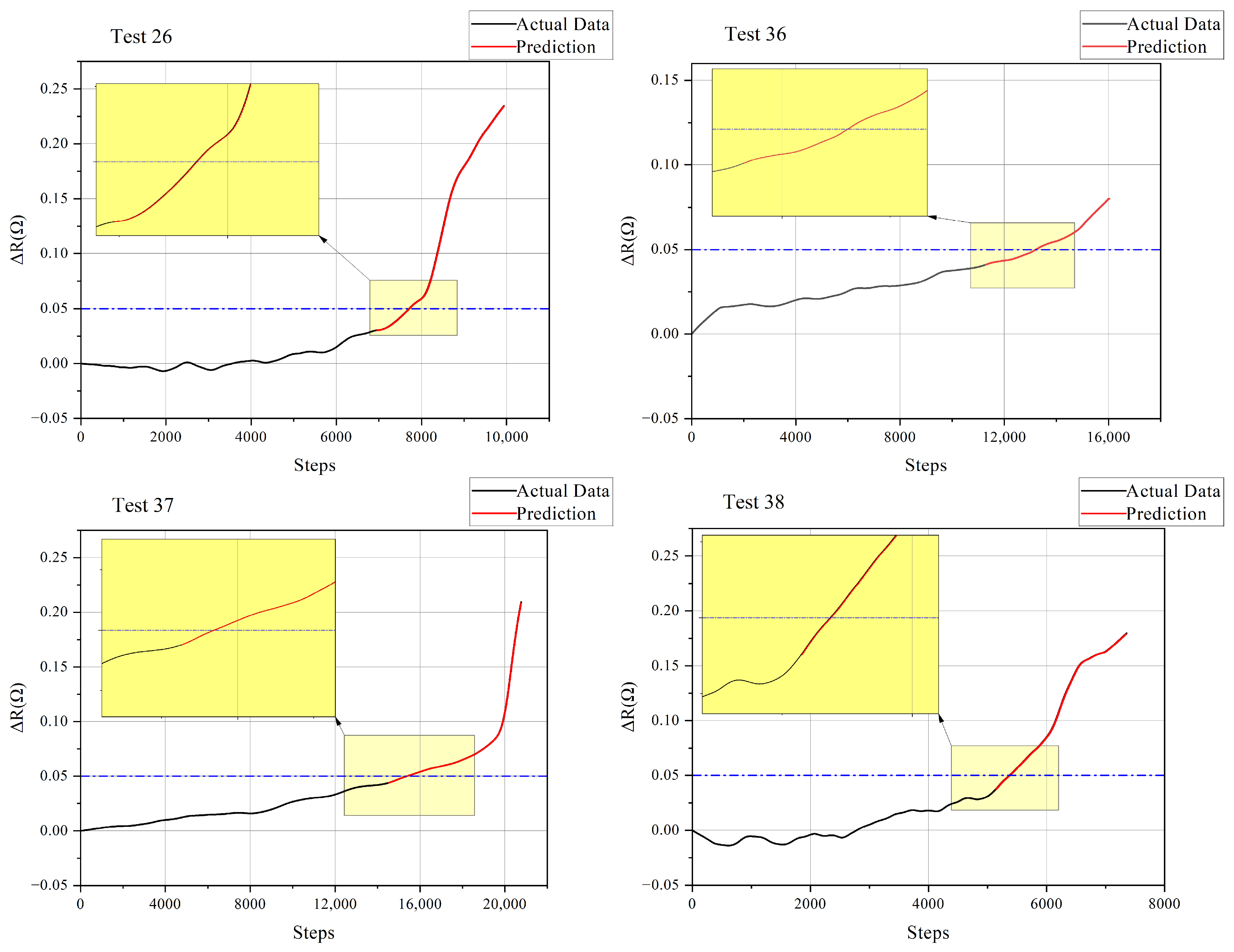
The prediction results for the four MOSFET test devices are presented in Figure 4. The measured $\Delta R_{\mathrm{ds}\left(\mathrm{on}\right)}$ trajectories are shown together with the multi-step forecasts generated by the proposed CNN–iTransformer model. The horizontal dashed lines denote the EOL criterion of $\Delta R_{\mathrm{ds}\left(\mathrm{on}\right)}$ = 0.05 Ω, and the insets enlarge the neighborhood around the threshold crossing so that the RUL-relevant region can be inspected more clearly. Both the measured and predicted curves in Figure 4 represent the signed on-state resistance drift after inverse standardization, expressed in ohms.

Figure 4. Model prediction results for different datasets. Black curves show observed history, and red curves show model predictions for Tests 26, 36, 37, and 38. Blue dashed lines mark the 0.05 Ω end-of-life threshold; yellow boxes and insets highlight the threshold-crossing regions.

Across the four reported records, the predicted trajectories generally follow the long-term increase in on-state resistance drift. Their agreement near the 0.05 Ω threshold supports the reported RUL estimate for Test 37. Because the sensitivity constraint is not a direct temporal-monotonicity constraint, local decreases in a forecast cannot be ruled out by the present formulation.

The quantitative results in Table 1 confirm the visual observations. Across the four test devices, the proposed model achieves an average MAE of 2.996 × 10⁻⁴, RMSE of 3.988 × 10⁻⁴, and RE of 3.110 × 10⁻³. This indicates that the model can provide highly accurate forecasts when the degradation trajectory evolves smoothly.

Table 1. Performance metrics of the proposed CNN–iTransformer model on four MOSFET test devices.

Test Device	MAE	RMSE	RE
Test 26	4.657 × 10−4	5.951 × 10−4	4.714 × 10−3
Test 36	1.127 × 10−4	1.205 × 10−4	1.166 × 10−3
Test 37	1.846 × 10−4	3.557 × 10−4	1.775 × 10−3
Test 38	4.353 × 10−4	5.240 × 10−4	4.784 × 10−3
Average	2.996 × 10−4	3.988 × 10−4	3.110 × 10−3

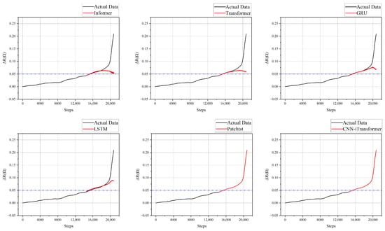
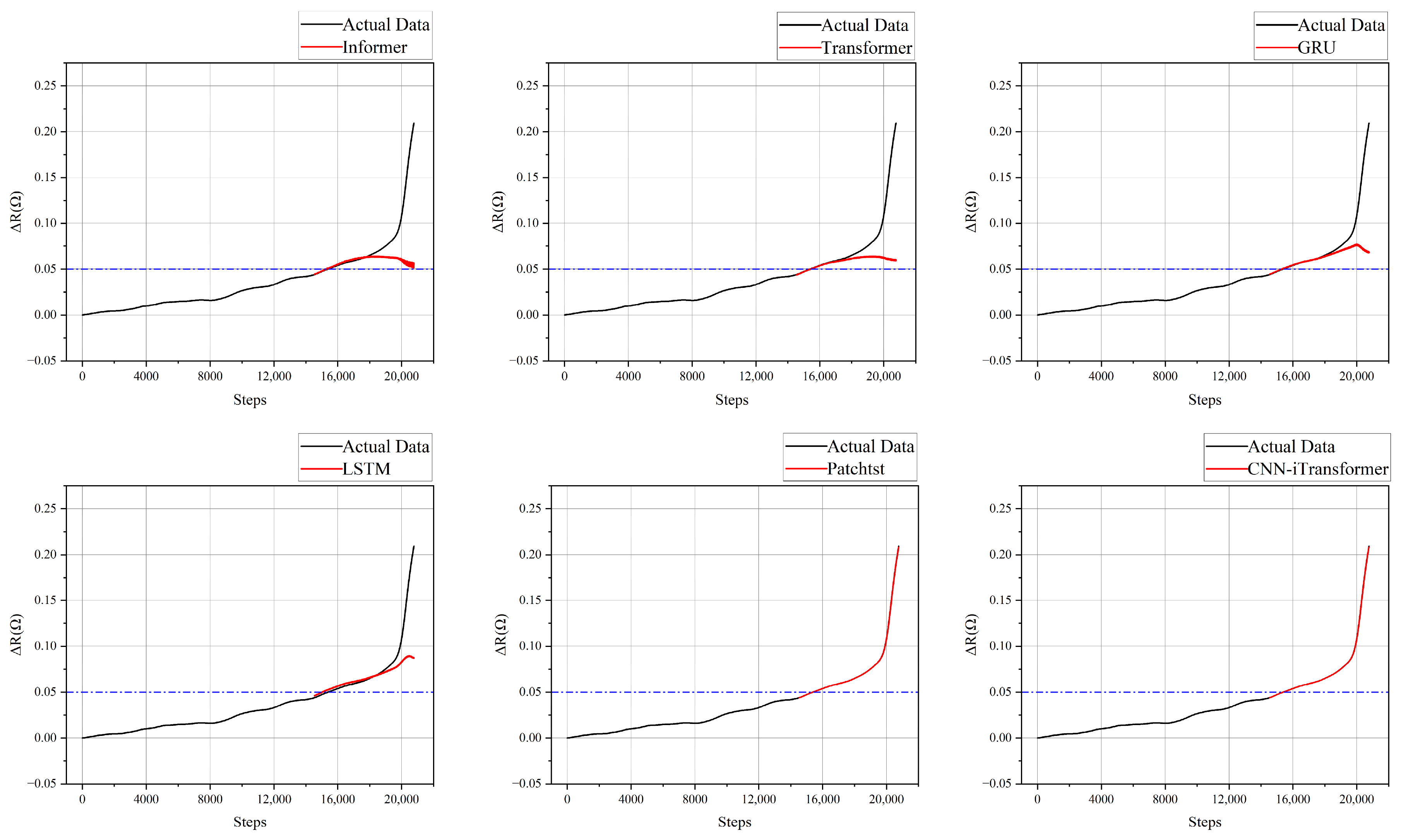
To further evaluate model competitiveness, the proposed method is compared with Informer, Transformer, GRU, LSTM, and PatchTST under the same prediction setting. The visual comparison in Figure 5 shows that conventional recurrent and attention-based baselines can approximate the mid-life trend but tend to underestimate or delay the final acceleration region. PatchTST provides the strongest baseline behavior, yet the proposed CNN–iTransformer more closely tracks the rapid rise of $\Delta R_{ds\left(on\right)}$ near the failure threshold.

Figure 5. Prediction results of the proposed method and the comparison methods. Black curves show measured data, and red curves show predictions. Blue dashed lines mark the 0.05 Ω end-of-life threshold.

Table 2 presents a quantitative comparison for the reported prediction setting. Relative to PatchTST, the proposed model has a lower reported MAE, RMSE, and RE in the shown comparison.

Table 2. Comparison of the different prediction methods.

Model	MAE	RMSE	RE
Informer	1.811 × 10−2	3.957 × 10−2	1.445 × 10−1
Transformer	1.759 × 10−2	3.810 × 10−2	1.410 × 10−1
GRU	1.358 × 10−2	3.361 × 10−2	9.859 × 10−2
LSTM	1.192 × 10−2	2.801 × 10−2	9.610 × 10−2
PatchTST	2.239 × 10−4	4.674 × 10−4	1.969 × 10−3
CNN–iTransformer	1.846 × 10−4	3.557 × 10−4	1.775 × 10−3

The direct RUL comparison in Table 3 is presented for Test 37. Its true RUL is 843 sampling steps, and the proposed model predicts 850 steps, corresponding to an absolute error of 7 steps, relative error of 0.83%, and precision of 99.17%. These values are specific to this record and prediction origin; the original manuscript does not provide direct RUL results for the other three reported records.

Table 3. RUL comparison of the different prediction methods.

Model	Predicted RUL	AERUL	RERUL (%)	PRUL (%)
Informer	702	141	16.73	83.27
Transformer	870	27	3.20	96.80
GRU	739	104	12.34	87.66
LSTM	450	393	46.62	53.38
PatchTST	852	9	1.07	98.93
CNN–iTransformer	850	7	0.83	99.17

The residual analysis of the four selected device-run records is summarized in Table 4. The complete test segments were evaluated to characterize the systematic bias and dispersion of the deterministic forecast errors across the datasets.

Table 4. Residual statistics of the CNN–iTransformer predictions.

Test Record	Mean Residual ($\overline{{\mathit{e}}_{\mathit{i}}}$)	Residual SD (${\mathit{s}}_{\mathit{e}\mathbf{,}\mathit{i}}$)
Test 26	4.66	3.70
Test 36	1.13	0.43
Test 37	1.85	3.04
Test 38	4.35	2.92

The mean residuals for Test 26, Test 36, Test 37, and Test 38 were 4.66 × 10⁻⁴, 1.13 × 10⁻⁴, 1.85 × 10⁻⁴, and 4.35 × 10⁻⁴ Ω, respectively. Their positive signs indicate a small but consistent tendency to underestimate the degradation magnitude. The corresponding residual standard deviations were 3.70 × 10⁻⁴, 0.43 × 10⁻⁴, 3.04 × 10⁻⁴, and 2.92 × 10⁻⁴ Ω. Thus, the deterministic forecast errors remain on the order of 10⁻⁴ Ω across the four records, although the observed positive residual bias should be considered when interpreting the point forecasts and derived RUL estimates. These empirical residual statistics characterize observed point-forecast errors and should not be interpreted as calibrated probabilistic prediction intervals.

The four selected records show small trajectory errors under the within-record evaluation. The reported comparison does not isolate gains from individual model components or establish transfer to new devices and operating conditions.

4.4. Discussion

The combination of convolutional feature extraction and attention over learned channels may help the model follow both local and longer-range degradation patterns. The reported comparisons do not establish which component produces the performance difference. The separate effects of LOWESS preprocessing and the physics-informed penalty have not been evaluated in a controlled comparison. The sensitivity penalty does not directly enforce temporal monotonicity of individual forecast steps.

The validation uses only four records from one accelerated-aging dataset, and the training portions of those same records are seen during model development. The results for independent experiments, different MOSFET technologies, and other operating conditions remain unknown. The model, therefore, remains dependent on the characteristics of the available training data, and device-disjoint validation is needed to assess transfer.

5. Conclusions

This work presents a physics-informed CNN–iTransformer framework for remaining useful life prediction of power MOSFETs using on-state resistance drift as the health indicator. The model combines a 1D convolutional module for local degradation pattern extraction with an iTransformer backbone for long-range sequence dependency modeling. A differentiable input-sensitivity penalty is incorporated into the training objective. The predicted $\Delta R_{ds\left(on\right)}$ trajectories are not guaranteed to be temporally monotonic.

On the four reported NASA thermal-overstress test records, the average MAE, RMSE, and RE were 2.996 × 10⁻⁴ Ω, 3.988 × 10⁻⁴ Ω, and 3.110 × 10⁻³, respectively. For Test 37, the reported predicted RUL was 850 sampling steps against the true value of 843, corresponding to a seven-step absolute error and 0.83% relative error. The comparisons indicate promising within-record forecasting under the studied conditions.

These findings support within-record forecasting on the studied thermal-overstress dataset. The current study is limited to univariate $\Delta R_{ds\left(on\right)}$ measurements from a single public accelerated-aging platform and has not yet been validated using an independent experimental setup. Other parameters, including threshold voltage, gate leakage current, and switching characteristics, may be more sensitive to gate-oxide-related degradation mechanisms. These parameters were not recorded in the selected thermal-overstress dataset and, therefore, cannot be included in the present feature-sensitivity analysis. Accordingly, the proposed framework should be interpreted as a prognostic method for die-attach-dominated degradation rather than as a universal model for all intrinsic and package-level MOSFET failure mechanisms. To address these limitations, future studies will establish an independent accelerated-aging test platform and expand the experimental matrix across additional devices by systematically varying thermal-cycling profiles, drain-current and drain-voltage stress levels, gate-drive voltage, frequency, and duty cycle, ambient temperature, and cooling conditions. The resulting datasets will be used to evaluate the robustness and cross-condition generalizability of the proposed framework.

The reported 99.17% RUL precision pertains only to Test 37 and is not the overall model accuracy. Future work should add a matched component ablation, device-disjoint validation, broader stress conditions, and additional health indicators when available.

References

- Chandel, M.; Rosenkranz, A.; Moraru, D.; Woźniak, A.; Jastrzębska, A.M. Measuring the Future—Nanometrology for Advanced Manufacturing of Miniaturized Devices. Adv. Funct. Mater. 2025, 35, 2501663. [Google Scholar] [CrossRef] [Scilit]
- Shao, L.; Xu, G.; Wei, W. Estimation Method for the Remaining Useful Life of Silicon Mosfets Based on Degradation Models and Deep Reflections on Its Technical Educational Requirements. J. Power Electron. 2026, 1–12. [Google Scholar] [CrossRef] [Scilit]
- Islam, R.; Rafin, S.M.S.H.; Mohammed, O.A. Comprehensive Review of Power Electronic Converters in Electric Vehicle Applications. Forecasting 2023, 5, 22–80. [Google Scholar] [CrossRef] [Scilit]
- Chandran, D.R.; Kumar, S.; Sanath, D. Solid State Transformers: A Comprehensive Review of Technology, Topologies, Applications, Research Gaps, and Future Directions. J. Power Energy Eng. 2025, 13, 30–64. [Google Scholar] [CrossRef]
- Handschuh-Wang, S.; Wang, T.; Gancarz, T.; Liu, X.; Wang, B.; He, B.; Dickey, M.D.; Wimmer, G.W.; Stadler, F.J. The Liquid Metal Age: A Transition from Hg to Ga. Adv. Mater. 2024, 36, 2408466. [Google Scholar] [CrossRef] [Scilit]
- Chaturvedi, A.; Sarma, M.; Chaturvedi, S.K.; Bernstein, J. Performance Assessment and RUL Prediction of Power Converters under the Multiple Components Degradation. Microelectron. Reliab. 2023, 144, 114958. [Google Scholar] [CrossRef] [Scilit]
- Zhang, J.F.; Gao, R.; Duan, M.; Ji, Z.; Zhang, W.; Marsland, J. Bias Temperature Instability of MOSFETs: Physical Processes, Models, and Prediction. Electronics 2022, 11, 1420. [Google Scholar] [CrossRef] [Scilit]
- Wang, P.; Zhao, Z. A Gate Oxide Degradation and Junction Temperature Evaluation Method for SiC MOSFETs Based on an On-State Resistance Model. Electronics 2025, 14, 2278. [Google Scholar] [CrossRef] [Scilit]
- Gao, L.; Liu, C.; Wu, F.; Qin, Y.; Wang, Y.; Huo, M. Prediction Method for the Remaining Useful Life of Power MOSFETs Based on Deep Learning. IEEE Trans. Power Electron. 2025, 40, 16676–16686. [Google Scholar] [CrossRef] [Scilit]
- Yi, J.; Ma, C.; Wang, H. A Data-Driven Remaining Useful Life Prediction Method for Power MOSFETs Considering Nonlinear Dynamical Behaviors. IEEE Trans. Electron Devices 2025, 72, 1885–1892. [Google Scholar] [CrossRef] [Scilit]
- Dusmez, S.; Duran, H.; Akin, B. Remaining Useful Lifetime Estimation for Thermally Stressed Power MOSFETs Based on On-State Resistance Variation. IEEE Trans. Ind. Appl. 2016, 52, 2554–2563. [Google Scholar] [CrossRef] [Scilit]
- Ni, Z.; Lyu, X.; Yadav, O.P.; Singh, B.N.; Zheng, S.; Cao, D. Overview of Real-Time Lifetime Prediction and Extension for SiC Power Converters. IEEE Trans. Power Electron. 2020, 35, 7765–7794. [Google Scholar] [CrossRef] [Scilit]
- Witczak, M.; Mrugalski, M.; Lipiec, B. Remaining Useful Life Prediction of MOSFETs via the Takagi–Sugeno Framework. Energies 2021, 14, 2135. [Google Scholar] [CrossRef] [Scilit]
- Wang, D.; Tsui, K.-L.; Miao, Q. Prognostics and Health Management: A Review of Vibration Based Bearing and Gear Health Indicators. IEEE Access 2018, 6, 665–676. [Google Scholar] [CrossRef] [Scilit]
- Mahapatra, S.; Sharma, U. A Review of Hot Carrier Degradation in N-Channel MOSFETs—Part I: Physical Mechanism. IEEE Trans. Electron Devices 2020, 67, 2660–2671. [Google Scholar] [CrossRef] [Scilit]
- Hou, X.; Luo, R.; Liu, Q.; Chi, Y.; Zhang, J.; Ma, H.; Zhang, Q.; Fan, J. High-Temperature Time-Dependent Dielectric Breakdown of 4H-SiC MOS Capacitors. Case Stud. Therm. Eng. 2024, 63, 105371. [Google Scholar] [CrossRef] [Scilit]
- Hu, Y.; Ge, H.; Ren, Z.; Yin, Y.; Zhao, R.; Chen, J. Threshold Voltage and Mobility Extraction of Negative Bias Temperature Instability in 22nm FD SOI MOSFETs. In Proceedings of the 2024 IEEE 17th International Conference on Solid-State & Integrated Circuit Technology (ICSICT); IEEE: New York, NY, USA, 2024; pp. 1–3. [Google Scholar]
- Ding, Y.; Liu, W.; Bai, W.; Tang, X.; Tang, N.; Yun, T.; Bai, Y.; Wang, Y.; Peng, Y.; Ma, Y.; et al. Modelling of SiC MOSFET Power Devices Incorporating Physical Effects. J. Power Electron. 2025, 25, 520–529. [Google Scholar] [CrossRef] [Scilit]
- Kao, M.-Y.; Kam, H.; Hu, C. Deep-Learning-Assisted Physics-Driven MOSFET Current-Voltage Modeling. IEEE Electron Device Lett. 2022, 43, 974–977. [Google Scholar] [CrossRef] [Scilit]
- Rajakumar, P.S.; Satheesh Kumar, S. A Comprehensive Review of Single Event Transients on Various MOS Devices. IEEE Access 2024, 12, 154760–154777. [Google Scholar] [CrossRef] [Scilit]
- He, Y.; Sang, L.; He, F.; Niu, X.; Li, X.; Dong, S.; Hao, X.; Li, Z.; Jin, R. SiC Hybrid Channel MOSFET with Low ON-Resistance and Low OFF-State Oxide Field. J. Power Electron. 2026, 1–7. [Google Scholar] [CrossRef] [Scilit]
- Kim, M.-K.; Yoon, Y.-D.; Yoon, S.W. Actual Maximum Junction Temperature Estimation Process of Multichip SiC MOSFET Power Modules with New Calibration Method and Deep Learning. IEEE J. Emerg. Sel. Top. Power Electron. 2023, 11, 5602–5612. [Google Scholar] [CrossRef] [Scilit]
- Liao, X.; Zhang, Q.; Du, W.; He, C.; Li, Y.; Wu, H. Switching Behavior Model for a SiC MOSFET Module Based on a Finite-State Machine. J. Power Electron. 2026, 26, 670–683. [Google Scholar] [CrossRef] [Scilit]
- Pugalenthi, K.; Park, H.; Raghavan, N. Prognosis of Power MOSFET Resistance Degradation Trend Using Artificial Neural Network Approach. Microelectron. Reliab. 2019, 101, 113467. [Google Scholar] [CrossRef] [Scilit]
- Chen, S.; Zhu, Y.; Konstantinou, G. Support Vector Regressor-Based SiC MOSFET Junction Temperature Prediction Based on Temperature Sensitive Electrical Parameters and External Dependencies. In Proceedings of the 2025 IEEE 16th International Symposium on Power Electronics for Distributed Generation Systems (PEDG); IEEE: New York, NY, USA, 2025; pp. 1187–1192. [Google Scholar]
- Hong, S.; Zhou, Z.; Lv, C.; Guo, H. Prognosis for Insulated Gate Bipolar Transistor Based on Gaussian Process Regression. In Proceedings of the 2013 IEEE Conference on Prognostics and Health Management (PHM); IEEE: New York, NY, USA, 2013; pp. 1–5. [Google Scholar]
- Murat Sezer, M.; Akici, F.; Afshar, M.; Teja Vankayalapati, B.; Akin, B. Gate Leakage Current Characterization and Remaining Useful Lifetime Prediction in Silicon Carbide MOSFETs. IEEE Trans. Transp. Electrif. 2025, 11, 8948–8958. [Google Scholar] [CrossRef] [Scilit]
- Baharani, M.; Biglarbegian, M.; Parkhideh, B.; Tabkhi, H. Real-Time Deep Learning at the Edge for Scalable Reliability Modeling of Si-MOSFET Power Electronics Converters. IEEE Internet Things J. 2019, 6, 7375–7385. [Google Scholar] [CrossRef]
- Ibrahim, M.S.; Abbas, W.; Waseem, M.; Lu, C.; Lee, H.H.; Fan, J.; Loo, K.-H. Long-Term Lifetime Prediction of Power MOSFET Devices Based on LSTM and GRU Algorithms. Mathematics 2023, 11, 3283. [Google Scholar] [CrossRef] [Scilit]
- Cheng, J.; Zhang, Y.; Cheng, X.; Guo, K.; Wang, Y.; Jiang, M.; Wang, Y.; Liu, Y. Thermal Behavior and Switching Losses of MOSFET in High-Frequency Transformer Circuits. Case Stud. Therm. Eng. 2025, 73, 106643. [Google Scholar] [CrossRef] [Scilit]
- Huang, J.; Wang, Y.; Li, Z.; Zhu, H.; Li, K. A Si IGBT/SiC MOSFET Hybrid Isolated Bidirectional DC–DC Converter for Reducing Losses and Costs of DC Solid State Transformer. Electronics 2024, 13, 801. [Google Scholar] [CrossRef] [Scilit]
- Chen, Y.; Zhou, Y.; Chen, J.; Ding, Q.; Yuan, H. Lifetime Prediction of SiC MOSFETs across Working Conditions Using Arrhenius and ProbSparse Transformer Residual Imputation. Microelectron. Reliab. 2026, 182, 116177. [Google Scholar] [CrossRef] [Scilit]
- Luo, W.; Liu, Y.; Pan, Y.; Bai, L. Remaining Useful Life Prediction of SiC MOSFETs Using the Autoformer-RELM Model. IEEE Trans. Instrum. Meas. 2025, 74, 2536811. [Google Scholar] [CrossRef] [Scilit]
- Nascimento, R.G.; Corbetta, M.; Kulkarni, C.S.; Viana, F.A.C. Hybrid Physics-Informed Neural Networks for Lithium-Ion Battery Modeling and Prognosis. J. Power Sources 2021, 513, 230526. [Google Scholar] [CrossRef] [Scilit]
- Shi, J.; Rivera, A.; Wu, D. Battery Health Management Using Physics-Informed Machine Learning: Online Degradation Modeling and Remaining Useful Life Prediction. Mech. Syst. Signal Process. 2022, 179, 109347. [Google Scholar] [CrossRef] [Scilit]
- Wen, P.; Ye, Z.-S.; Li, Y.; Chen, S.; Xie, P.; Zhao, S. Physics-Informed Neural Networks for Prognostics and Health Management of Lithium-Ion Batteries. IEEE Trans. Intell. Veh. 2024, 9, 2276–2289. [Google Scholar] [CrossRef] [Scilit]
- Ye, J.; Xie, Q.; Lin, M.; Wu, J. A Method for Estimating the State of Health of Lithium-Ion Batteries Based on Physics-Informed Neural Network. Energy 2024, 294, 130828. [Google Scholar] [CrossRef] [Scilit]
- Xie, Y.; Zhang, Y.; Miao, Q. Remaining Useful Life Prediction of Power MOSFETs Based on Deep Reinforcement Learning. IEEE Sens. J. 2025, 25, 35090–35100. [Google Scholar] [CrossRef] [Scilit]
- Alzubaidi, L.; Zhang, J.; Humaidi, A.J.; Al-Dujaili, A.; Duan, Y.; Al-Shamma, O.; Santamaría, J.; Fadhel, M.A.; Al-Amidie, M.; Farhan, L. Review of Deep Learning: Concepts, CNN Architectures, Challenges, Applications, Future Directions. J. Big Data 2021, 8, 53. [Google Scholar] [CrossRef] [Scilit]
- Liu, Y.; Hu, T.; Zhang, H.; Wu, H.; Wang, S.; Ma, L.; Long, M. iTransformer: Inverted Transformers Are Effective for Time Series Forecasting. arXiv 2024, arXiv:2310.06625. [Google Scholar]
- Celaya, J.R.; Saxena, A.; Saha, S.; F. Goebel, K. Prognostics of Power MOSFETs under Thermal Stress Accelerated Aging Using Data-Driven and Model-Based Methodologies. Annu. Conf. Progn. Health Manag. Soc. 2011, 3, 1–10. [Google Scholar] [CrossRef] [Scilit]
Disclaimer/Publisher’s Note: The statements, opinions and data contained in all publications are solely those of the individual author(s) and contributor(s) and not of MDPI and/or the editor(s). MDPI and/or the editor(s) disclaim responsibility for any injury to people or property resulting from any ideas, methods, instructions or products referred to in the content. |
© 2026 by the authors. Licensee MDPI, Basel, Switzerland. This article is an open access article distributed under the terms and conditions of the Creative Commons Attribution (CC BY) license.