Hierarchical Balanced Pseudo-Label Random Forest for Imbalanced Industrial Process Fault Classification Under Limited Labels

Abstract

Objective: This study addresses multiclass industrial fault classification when human labels are simultaneously scarce and class-imbalanced. The proposed hierarchical balanced pseudo-label random forest (HBPL-RF) is novel in coordinating class-adaptive confidence cut-points and per-class pseudo-label quotas with class-balanced forests, validation gating and rollback, soft fusion under extreme label scarcity, and a rare-fault-first decision branch. HBPL-RF was evaluated on the Cranfield multiphase-flow and Tennessee Eastman benchmarks at five labeled fractions and five random seeds. It produced the highest observed mean Macro F1 under the unified protocol: 0.7324 on Cranfield and 0.6109 on Tennessee Eastman. At the nominal 1% Cranfield level, the primary cross-validation-feasible allocation contains five labeled Case 6 windows per seed to support five-fold validation and yields Case 6 F1 = 0.6627 ± 0.0458. Under strict proportional sampling with three Case 6 labels, F1 falls to 0.4019 ± 0.0718; the primary value therefore must not be interpreted as ordinary proportional 1% random labeling. Capacity-matched controls, ablations, sensitivity analysis, and error decomposition are consistent with the intended class-control and rare-fault-protection mechanisms, but do not establish causal effects or universal superiority. The conclusions are restricted to the two benchmarks, declared labeling protocols, and experimental conditions studied.

1. Introduction

Complex industrial processes exhibit nonlinear coupling, dynamic lags, and operating-condition changes, while confirmed fault labels require expert records, controlled injections, maintenance evidence, or shutdown analysis. Quantitative characteristics reported in the benchmark literature illustrate this mismatch: the Cranfield facility records 24 process variables at 1 Hz across normal operation and six injected fault cases [1], whereas the Tennessee Eastman benchmark defines 21 fault cases plus normal operation over 52 measured and manipulated variables [2]. Reviews of data-driven monitoring emphasize that realistic diagnosis must address label scarcity, imbalance, and reproducible evaluation rather than accuracy alone [3]. Open-benchmark analysis likewise warns that differences in split construction and preprocessing can make cross-paper headline metrics incomparable [4].

Random forests learn nonlinear class boundaries through bagging and feature subsampling [5]. Gradient-boosting trees and neural representations provide alternative nonlinear learners, but their reported effectiveness still depends on the number, balance, and provenance of labeled examples [6]. Transfer learning can reduce supervision requirements when source and target domains are compatible [7], and chemical-process classifiers can exploit process-specific feature structure [8]. Neither strategy by itself prevents a rare class from contributing too few labeled or pseudo-labeled examples to influence the final boundary.

Semi-supervised learning exploits unlabeled observations alongside a small, labeled set [9], and self-training provides a classifier-agnostic implementation [10]. The central risk is confirmation bias: early errors can be returned to the training pool as if they were labels [11]. FixMatch filters predictions through confidence and consistency [12]; FlexMatch adapts acceptance during training [13]; FreeMatch makes the confidence cut-point self-adaptive [14]; and distribution-aware pseudo-labeling explicitly considers class imbalance [15]. Reviews of class-imbalanced semi-supervised learning show that confidence quality and the class composition of accepted samples must be considered together [16]. Industrial studies have consequently combined uncertainty analysis [17], class-information screening [18], and semi-supervised ensembles [19], but they do not provide the same coordinated class-wise threshold, growth cap, rollback, and hierarchical rare-fault mechanism used here.

Recent industrial-process methods strengthen feature learning through self-supervision, graph structure, and spatio-temporal latent variables. S4FD combines self-supervised and semi-supervised objectives [20]. FIGNN introduces fuzzy-inference-guided graph propagation [21]. SS-STGVAE learns spatio-temporal graph variational representations [22], and SsMsGNN integrates multiple graph scales [23]. These methods are strong representation-oriented comparators, but representation capacity does not itself guarantee balanced pseudo-label admission. Table 1 therefore reports both the unified-protocol quantitative comparison and the functional difference relevant to the present research gap.

Table 1. Quantitative and functional comparison of representative recent methods under the unified protocol used in this study.

Method/Source	Primary Mechanism	Cranfield Mean Macro F1	TE Mean Macro F1	Gap Relative to HBPL-RF
S4FD [20]	Self-supervision-enhanced semi-supervised diagnosis	0.6987	0.5849	No explicit per-class pseudo-label growth cap, rollback, or rare-fault priority branch
FIGNN [21]	Fuzzy-inference-guided graph neural network	0.6895	0.5822	Representation guidance without the complete class-wise acceptance-control stack
SS-STGVAE [22]	Spatio-temporal graph variational representation	0.7052	0.5904	No explicit coordination of class quota, rollback, and rare-fault override
SsMsGNN [23]	Semi-supervised multiscale graph neural network	0.7120	0.5963	Strongest compared deep baseline; no matched hierarchical rare-fault mechanism
HBPL-RF (this study)	Balanced forests plus class-controlled self-training and hierarchical decision	0.7324	0.6109	Integrates class-wise quality and quantity control with update gating and rare-fault priority

Note: The two Macro F1 columns are averages over the five labeled fractions obtained under this study’s unified evaluation protocol, not values copied from heterogeneous source-paper protocols. The table is descriptive; small mean differences are not claims of statistical superiority.

HBPL-RF addresses this gap through class-wise quality-quantity control. Adaptive confidence cut-points regulate which unlabeled candidates are eligible, while per-class quotas cap how rapidly each predicted class can expand. Class-balanced forest fitting increases minority participation; training-internal validation gating with rollback governs update retention; soft fusion attenuates uncertain pseudo-labels at the nominal 1% level; and a hierarchical rare-fault branch gives engineering-critical faults a priority decision path. The contributions are as follows: (1) a tree-based semi-supervised framework that jointly controls pseudo-label quality and class-wise growth; (2) a validation-controlled update mechanism with rollback and extreme-label soft weighting; (3) a rare-fault-first branch that is isolated through matched-capacity and removal controls; and (4) a two-benchmark evaluation with five label regimes, five outer seeds, strict proportional sensitivity, ablation, parameter sensitivity, error analysis, uncertainty analysis, and computational cost reporting.

2. Materials and Methods

2.1. Random Forest Base Model

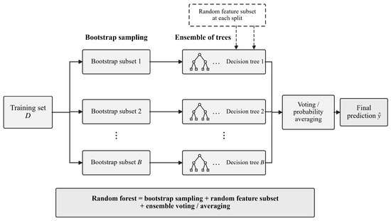
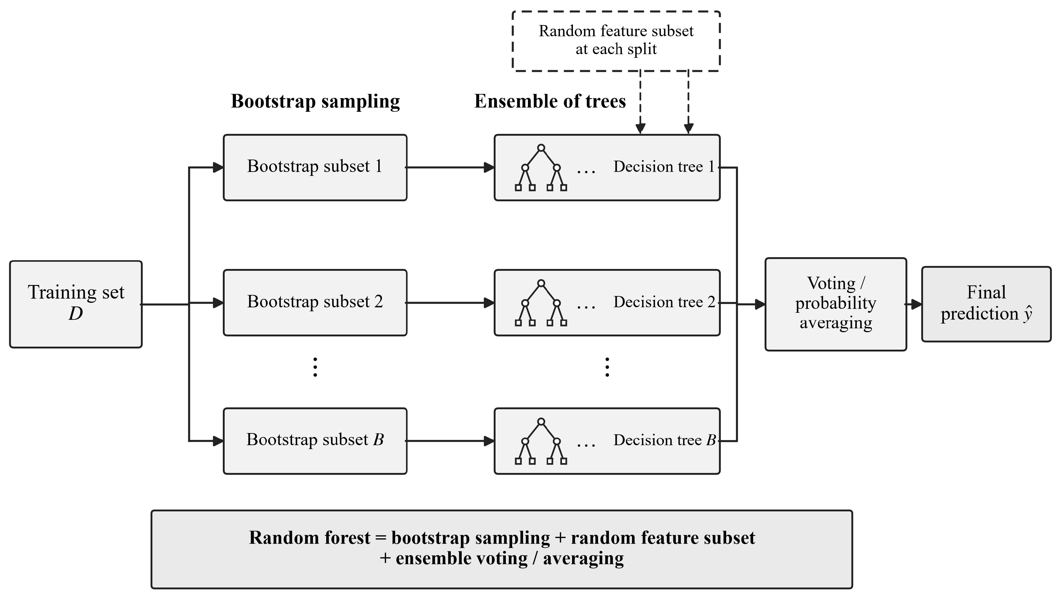
Random forest is a bagged ensemble [5]. Each tree is fitted to a bootstrap sample and considers a random feature subset at each split. In the implementation used here, a tree’s class score is the labeled-class fraction in the reached leaf, and the forest score is the average across trees. These vote-averaged scores support ranking, pseudo-label screening, and final classification; they are confidence scores and are not asserted to be calibrated posterior probabilities. This distinction matters because threshold transfer under class-prior shift requires separate calibration evidence.

Let the forest contain B trees. For tree b, let p_b(c|x) denote its class-c confidence score for sample x. The forest’s vote-averaged class score is

$$\widehat{p}\left(c\mid x\right)={\displaystyle \frac{1}{B}}{\displaystyle {\sum }_{b=1}^B}{p}_b\left(c\mid x\right), c\in C$$

(1)

where x is the input sample; c is a candidate fault class; C is the class set; B is the number of trees; b is the tree index; and p_b(c|x) is the class-c tree score. The predicted class is

$$\widehat{y}=f_{\mathrm{RF}}\left(x\right)=\arg \underset{c\in C}{\max }\widehat{p}\left(c\mid x\right)$$

(2)

Ordinary random forests capture nonlinear feature interactions, but, with extremely few and imbalanced labels, majority classes may participate more often in splitting and minority boundaries may be weakly represented. HBPL-RF therefore modifies bootstrap construction, pseudo-label admission, update control, and hierarchical decision-making. Baseline RF, CBRF, and ST-RF use 500 trees; HBPL-RF uses 500 trees per self-training fit and a final three-member ensemble of 800 trees per member, as detailed in Section 2.9. The basic random-forest structure is illustrated in Figure 1.

Figure 1. Basic structure of the random forest. Solid boxes denote data/model components, solid arrows denote processing flow, the dashed box denotes random feature selection at each split, and ellipses indicate repeated bootstrap subsets or trees.

2.2. Semi-Supervised Pseudo-Labeling and Class-Imbalance Learning

Semi-supervised learning jointly uses a small, labeled set and a much larger unlabeled set [9]. In ordinary pseudo-label self-training, an initial classifier predicts labels for unlabeled samples, and high-confidence predictions are added to the training set [10]. The approach is simple and compatible with random forests, but it can amplify confirmation bias when the initial classifier is biased.

Class-imbalance learning includes undersampling [24], resampling and weighting [25], and data-level generation [26]. Under limited-label semi-supervised fault classification, minority classes have both fewer human labels and fewer high-confidence pseudo-labels, so one global cut-point can make majority pseudo-labels accumulate faster. FixMatch [12], debiased self-training [27], FlexMatch [13], distribution-aware pseudo-labeling [15], FreeMatch [14], class-reweighted semi-supervised learning [28], kernel alignment [29], TrustMatch [30], and uncertainty-aware adaptive thresholds for fault diagnosis [31] offer complementary controls. HBPL-RF focuses specifically on coordinating class-wise admission quality, relative population growth, update rollback, and engineering-prior rare-fault protection.

2.3. Task Definition and Feature Representation

Let L denote the labeled training set, U the unlabeled training set, and T the independent labeled test set. Each sample is represented by a feature vector x and, when labeled, a class label y. The goal is to learn a classifier f from L and U that achieves high Macro F1 and balanced accuracy on T without using test-set information during feature standardization, model selection, threshold adjustment, rare-class selection, or pseudo-label screening.

For Cranfield, each process window is represented by nine statistics computed from 24 process variables: mean, standard deviation, minimum, maximum, median, root mean square, 25th percentile, 75th percentile, and linear-trend slope. The k-th window feature vector is

x_k = concat[φ₁(Z_k), φ₂(Z_k),…, φ_m(Z_k)] ∈ ℝ²¹⁶

(3)

where Z_k is the k-th process window and φ_j(·) is the j-th statistical-feature operator. For Cranfield, each operator returns one statistic for each of the 24 process variables, so φ_j(Z_k) ∈ ℝ²⁴. With m = 9, the window vector is formed by concatenation, x_k = concat[φ₁(Z_k),…, φ_m(Z_k)] ∈ ℝ²¹⁶, as written in Equation (3). TE uses the original 52-dimensional process-variable representation. The mean and standard deviation used for continuous-feature standardization are estimated only from the training split and then applied unchanged to validation and test samples.

2.4. Overall HBPL-RF Framework

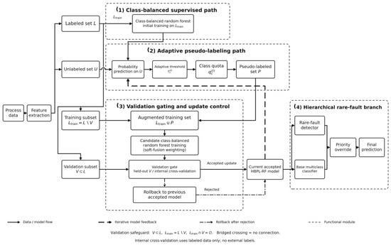
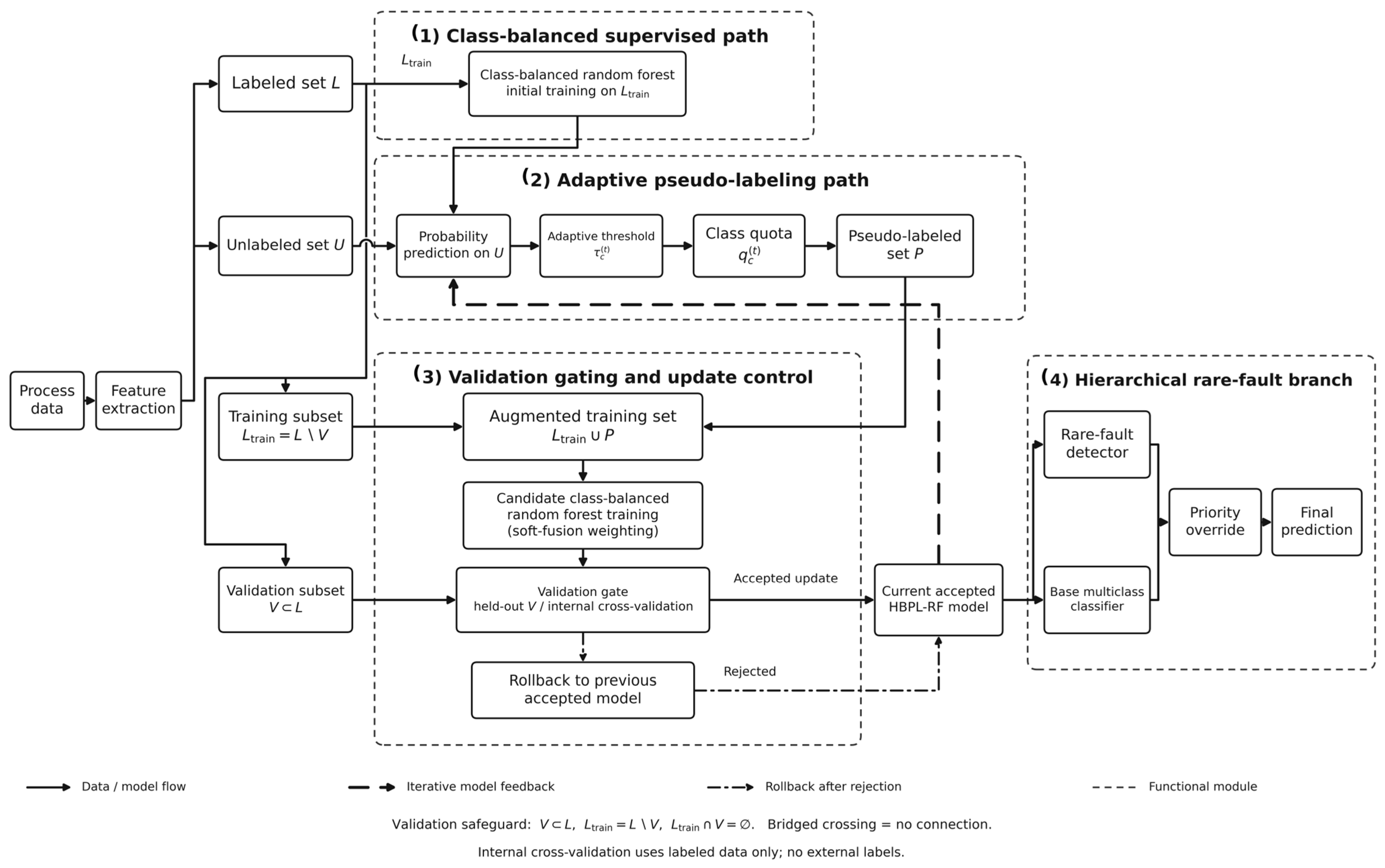
Figure 2 shows the overall HBPL-RF architecture. HBPL-RF contains four coordinated paths: (1) a class-balanced supervised path that constructs an initial minority-aware decision boundary; (2) an adaptive pseudo-label path that screens unlabeled samples using class-wise confidence thresholds and per-class quotas; (3) a validation-gating path that accepts or rejects self-training updates and enables rollback or soft fusion; and (4) a hierarchical rare-fault branch that prioritizes engineering-critical minority faults. The internal validation/CV observations shown in Figure 2 are carved exclusively from the declared labeled set L and therefore do not constitute an additional labeled dataset.

Figure 2. Overall framework of HBPL-RF. Internal validation/CV observations are carved exclusively from the declared labeled set L.

2.5. Class-Balanced Supervised Path

In self-training round t, let L^(t) denote the current labeled-plus-accepted training pool and L_c^(t) its class-c subset, with n_c^(t) = |L_c^(t)|. For each tree b and each class c, Sample(·) draws s_t instances from the current class set with replacement. For the reported experiments, s_t = min_c∈C n_c^(t), i.e., the minimum current class size at round t; the same s_t is used for every class within a tree and is recomputed after each accepted self-training update. If an instance is drawn more than once for the same tree, the duplicate draws are retained as separate bootstrap occurrences, so their multiplicity contributes to that tree in the same way as ordinary bootstrap resampling. The class-balanced tree subset is therefore

$${\mathcal{B}}_b^{\left(t\right)}=\underset{c\in C}{⨄}\mathrm{Sample}\left(L_c^{\left(t\right)},s_t\right)$$

(4)

Here, the n-ary multiset-union/concatenation operator preserves repeated bootstrap occurrences rather than collapsing them as an ordinary set union would. This balanced bootstrap does not alter the true test distribution. Instead, it increases minority-class participation during tree construction so that rare classes can form candidate decision boundaries even under extremely low labels. The procedure is performed independently for every tree.

2.6. Adaptive Threshold and Class Quota

Ordinary self-training accepts an unlabeled sample when its largest model confidence exceeds one global cut-point. HBPL-RF instead uses a class-wise operational cut-point determined by current class size:

$${\tau }_c^{\left(t\right)}=\mathrm{clip}\left[{\tau }_0+\lambda \ln \left({\displaystyle \frac{n_c^{\left(t\right)}+\epsilon }{{\bar{n}}^{\left(t\right)}+\epsilon }}\right),{\tau }_{\min },{\tau }_{\max }\right]$$

(5)

where n_c(t) is the current size of class c, $\bar{\mathrm{n}}$(t) is the mean class size in the labeled-plus-accepted pool, τ₀ is the base cut-point, λ controls class adaptation, ε prevents division by zero, and clipping restricts the value to [τ_min, τ_max]. A majority class is therefore assigned a stricter operational cut-point, while a minority class can receive a moderately relaxed one. These values are selected using training-internal validation and are not probability-calibration parameters.

HBPL-RF also limits the number of accepted pseudo-labels for each class in each round:

$$q_c^{\left(t\right)}=\max \left(q_{\min },⌈\rho n_c^{\left(t\right)}⌉\right), \left|{\mathcal{P}}_c^{\left(t\right)}\right|\le q_c^{\left(t\right)}$$

(6)

where n_c^(t) is the size of class c in the current labeled-plus-accepted training pool, q_min is the admission floor, ρ is the nominal per-round relative-growth ratio, and P_c^(t) denotes the set of class-c pseudo-labels accepted in round t. Equation (6) enforces |P_c^(t)| ≤ q_c^(t); it is not an equal-count allocation. Apart from the q_min floor, it caps each class’s relative growth at approximately ρ per round. The class-balancing effect is joint: Equation (5) controls admission quality by relaxing minority-class thresholds and tightening majority-class thresholds, Equation (6) controls admission quantity by limiting relative class expansion, and Equation (4) gives classes equal sampling contribution during tree construction. Consequently, high confidence alone cannot make a majority class expand without a per-round cap, while a minority class can receive a moderately relaxed threshold without unlimited admission. The methodological emphasis is therefore the coupled class-level control of pseudo-label quality and relative population growth, rather than any individual thresholding or resampling component in isolation. When eligible candidates exceed the quota, the highest-confidence candidates are retained; HBPL-RF therefore does not require identical accepted pseudo-label counts across classes.

2.7. Validation Gating, Rollback, and Soft Fusion

When the labeled fraction is sufficiently large, an internal validation set is used to determine whether a pseudo-label update is accepted. An update is retained only when its validation Macro F1 does not fall below the best historical value by more than the tolerance δ:

$$A^{\left(t\right)}=\left\{\begin{array}{ll}1,& M_{\mathrm{val}}^{\mathrm{new}}\ge M_{\mathrm{val}}^{\mathrm{best}}-\delta ,\\ 0,& \mathrm{otherwise}\end{array}\right.$$

(7)

If the gate rejects an update, the model rolls back to the previous best state. Under the nominal 1% labeled condition, a fixed holdout validation set is too small and unstable. HBPL-RF therefore estimates the pseudo-label gain ΔM by stratified 5-fold cross-validation. For each fold, the pseudo-label generator and candidate model are fitted using human labels from the other four folds only; the held-out fold labels are used exclusively to compute validation Macro F1 and do not enter pseudo-label generation or model fitting for that fold. Thus, ΔM is estimated in a fold-wise out-of-fold manner. Cranfield fold assignment follows the group-aware non-overlap rule specified in Section 2.9. For Cranfield, the primary nominal 1% allocation contains five labeled Case 6 windows and assigns one to each held-out fold, subject to the group-aware non-overlap rule; consequently, each validation fold contains one Case 6 sample and each corresponding fitting portion contains four. The 1% update is accepted when the mean 5-fold cross-validation change satisfies ΔM ≥ −0.0020; an update with ΔM < −0.0020 is rejected and the previous accepted model state is restored. For accepted 1% updates, pseudo-labeled samples are assigned a confidence-and-gain-dependent weight:

$$w_i=\max \left[w_{\min },\sigma \left({\displaystyle \frac{\Delta M}{T_s}}\right)\right]·\underset{c\in C}{\max }\widehat{p}\left(c\mid x_i\right)$$

(8)

where w_min is the floor applied to the validation-gain factor inside the max operator, σ(·) is the sigmoid, ΔM is the cross-validation Macro F1 change, and T_s is the temperature. Thus, w_min is not a lower bound on the final sample weight w_i: multiplication by model confidence can make w_i smaller than w_min. Human-labeled observations receive weight 1.0, whereas accepted pseudo-labeled observations receive w_i.

After class-balanced bootstrap construction, sample weights are supplied to each tree fit and enter weighted impurity calculations without altering bootstrap multiplicity. Soft fusion is therefore intended to attenuate uncertain pseudo-labels rather than treating every accepted candidate equally. Under the reported nominal 1% acceptance rule, the gain-factor floor is only a numerical safeguard. In the ablation that disables validation gating while retaining soft fusion, ΔM is computed only for Equation (8) weighting; accept/reject gating and rollback are disabled.

2.8. Hierarchical Rare-Fault Branch

Let R denote the set of engineering-important faults that require priority recognition. For each sample x, let r denote the rare class in R with the largest branch score g_r(x). HBPL-RF first evaluates this rare-fault branch and returns that highest-scoring rare class only when its score reaches the branch threshold; otherwise, the base multiclass classifier h(x) is used:

$$f_H\left(x\right)=\left\{\begin{array}{ll}\underset{r\in \mathcal{R}}{\mathrm{argmax}}{g}_r\left(x\right),& \underset{r\in \mathcal{R}}{\max }{g}_r\left(x\right)\ge {\theta }_R,\\ h\left(x\right),& \mathrm{otherwise}\end{array}\right.$$

(9)

For Cranfield, R = {Case 6}. This set was fixed before external test evaluation from engineering risk, sample scarcity, and prior field importance of the 2-inch (50.8 mm) line-pressurization fault; it was not selected from test performance. For TE, rare classes are selected only from training-internal validation or cross-validation. Eligible classes have at least two positive and two negative observations, are ranked by validation per-class F1, and the four lowest-F1 eligible classes are retained. Each one-versus-rest detector uses 500 trees, unrestricted depth, max_features = sqrt, minimum leaf size 2, balanced_subsample weighting, and random state seed + 1000 + 37r. The branch values g_r(x), like $\widehat{\mathrm{p}}$(c|x), are vote-averaged RF confidence scores rather than calibrated probabilities. The operational branch cut-points are θ_R = 0.40 for Cranfield and 0.35 for TE. When the largest rare-class score reaches θ_R, the priority branch returns that rare class; otherwise, the full multiclass model h(x), which still includes all rare classes, provides the prediction. Deployment under prior or operating-condition drift would require calibration and periodic cut-point reassessment. The complete HBPL-RF training procedure is summarized in Table 2.

Table 2. Training procedure of HBPL-RF.

Item	Algorithm Step
Input	Labeled set L, unlabeled set U, class set C, rare-fault set R, base threshold τ0, quota ratio ρ, and maximum iterations T.
1	Construct process features and split the training pool into labeled and unlabeled subsets according to the declared labeled fraction. Validation/CV labels are carved exclusively from the declared labeled subset, with no additional labeled samples introduced.
2	Train the current class-balanced RF using per-class bootstrap sampling with replacement as defined in Equation (4).
3	For round t = 1,…,T, predict vote-averaged class confidence scores for the remaining unlabeled samples U.
4	For each class c, compute the adaptive threshold τ_c and class quota q_c; keep only candidates satisfying the class threshold and retain the highest-confidence candidates up to q_c.
5	Form the candidate augmented training set. For labeled fractions ≥5%, evaluate the update on the internal validation set; under nominal 1% labels, estimate ΔM by fold-wise out-of-fold 5-fold cross-validation according to the dataset-specific partition rule in Section 2.9, apply the 1% acceptance rule ΔM ≥ −0.0020, and compute the soft-fusion weight in Equation (8).
6	Accept an update only when it satisfies the applicable holdout/CV gate; otherwise roll back to the best previous state. Continue until the maximum number of rounds is reached.
7	Determine the rare-fault set using the predefined Cranfield engineering prior or training-only validation/cross-validation for TE; the test set is never used for rare-class selection.
8	Train the rare-fault branch and the base multiclass branch from the final accepted training state and apply the hierarchical decision rule in Equation (9).
Output	Final hierarchical HBPL-RF classifier and the saved round-by-round diagnostic log.

2.9. Datasets, Splits, Hyperparameter Selection, and Reproducibility

Table 3 summarizes the two benchmark datasets, fixed external test settings, and labeled-fraction regimes used in all experiments.

Table 3. Datasets, external test splits, and labeled-fraction regimes.

Dataset	Classes	Features/Variables	Training Samples	Test Setting	Nominal Labeled Fraction
Cranfield	7	Window statistics of 24 variables (216 features)	6646 windows	Fixed cross-run test; 4652 windows; train/test = 58.8%/41.2%	1%, 5%, 10%, 20%, 50%
TE	22	52-dimensional process features	10,580 samples	Test0–Test21; transition rows removed from Test1–Test21; 17,760 samples; train/test = 37.3%/62.7%	1%, 5%, 10%, 20%, 30%

The Cranfield data originate from the Three-Phase Flow Facility at Cranfield University, UK [1]. The rig transports single-phase or mixed water, oil, and air through a pressurized pipeline system containing multiple pipe geometries, a 10.5 m riser, separators, tanks, pumps, air supply, regulating valves, and a DeltaV supervisory control and data acquisition system. The original records contain 24 process variables sampled at 1 Hz. Normal data contain three variable-flow operating groups (T1, T2, and T3), and six manually injected fault types are available: air-line blockage, water-line blockage, top gas–liquid separator inlet blockage, mistaken bypass-valve opening, slugging, and 2-inch line pressurization.

To avoid optimistic evaluation caused by run overlap, Cranfield uses isolation by independent acquisition runs. T3, Set1_3, Set2_3, Set3_3, Set4_3, Set5_2, and Set6_2 are fixed as test groups; all remaining runs form the training pool. After windowing, the split contains 6646 training and 4652 external test windows, corresponding to 58.8% and 41.2% of the 11,298 analyzed windows. A window length of 60 and a step of 10 are used, and mixed windows crossing fault boundaries are excluded when the target-fault proportion is below 0.80. Training counts are 1843, 1072, 986, 918, 874, 661, and 292; test counts are 1290, 751, 690, 643, 612, 463, and 203. Case 6 is 4.39% of the training pool. The primary nominal 1% labeled subset fixes Case 6 at five windows solely to make five-fold validation feasible, then allocates the remaining 62 labels proportionally across Classes 0–5. This allocation rule does not use test outcomes but raises the Case 6 labeled share to 7.46%; Section 3.2 therefore reports the strict proportional three-label sensitivity.

For transparent label-budget accounting, the exact Cranfield labeled counts are as follows: 1%: 67 total = [18, 10, 10, 9, 9, 6, 5]; 5%: 332 = [92, 54, 49, 46, 44, 33, 14]; 10%: 665 = [184, 107, 99, 92, 87, 66, 30]; 20%: 1329 = [369, 214, 197, 184, 175, 132, 58]; and 50%: 3323 = [922, 536, 493, 459, 437, 331, 145], where entries are Classes 0–6. The validation/CV observations are drawn exclusively from the declared labeled subset and therefore introduce no additional labeled observations. Under the primary nominal 1% condition, the declared total labeled budget remains 67 windows per seed, including the five Case 6 windows required by the 5-fold validation procedure.

The Tennessee Eastman benchmark follows Downs and Vogel [2] and uses 41 measured plus 11 manipulated variables, one normal class, and 21 fault classes. Its training pool contains 10,580 observations: 500 normal and 480 for each fault. Test0 contributes 960 normal observations. For Test1–Test21, the first 160 rows are removed as pre-fault/transition observations, leaving 800 post-transition observations per fault and 17,760 test observations in total. Relative to the combined 28,340 analyzed observations, the declared training and test portions are 37.3% and 62.7%, respectively. These fixed external test files are never used for tuning or pseudo-label screening.

Both datasets are evaluated with five random seeds. The exact seed set is {17, 29, 43, 71, 113}. For each nominal labeled fraction, the labeled and unlabeled subsets are regenerated by stratified sampling, while the external test groups remain fixed. Because stratified sampling and cross-validation require integer per-class counts, the listed fractions are nominal targets. The nominal 1% allocations are 67/6646 = 1.0081% for Cranfield, including five Case 6 windows so that each of the five held-out folds contains one positive, and 110/10,580 = 1.0397% for TE, using a minimum of five labels per class to permit class-stratified 5-fold cross-validation. All validation/CV samples remain inside these declared labeled budgets. The test data do not participate in standardization, threshold adjustment, rare-class selection, model selection, or pseudo-label screening. The maximum labeled fractions were selected so that the largest labeled sets are comparable in absolute size: approximately 3323 Cranfield windows at 50% and 3174 TE samples at 30%.

Hyperparameters are selected independently for Cranfield and TE using only their training pools. Candidate ranking uses mean training-internal Macro F1, with ties within 0.001 resolved in favor of the lower-capacity or more conservative setting. The staged search in Table 4 avoids an infeasible full Cartesian product: confidence control is screened first, followed by quota/update settings, gating/fusion settings, the rare-branch cut-point, and the shortlisted RF capacity. The arrow (→) in Table 4 denotes the stated tie-breaking preference. The staged search evaluated 60 candidate configurations per dataset for the nominal 1% regime, 52 per dataset for each standard regime of at least 5%, and 57 for the dedicated Cranfield 50% regime. These totals count the configurations actually fitted across the sequential stages, rather than a Cartesian-product total. Development random states {1017, 1029, 1043, 1071, 1113} were used to rank candidates, while the final external test runs use outer seeds {17, 29, 43, 71, 113}. Candidate values are shared where the data representation permits, but selection is performed separately for the two datasets. Once selected, one configuration is frozen across the five final outer seeds; external test labels are never used for ranking, early stopping, threshold selection, rare-class selection, or rollback.

Table 4. Training-internal hyperparameter search space and selection rule.

Stage/Parameter	Candidate Values	Selection Scope	Rule
Confidence: τ0	1%: 0.70, 0.74, 0.78, 0.82, 0.86; ≥5%: 0.75, 0.80, 0.85, 0.90, 0.95	Independent by dataset and label regime	Maximize mean internal Macro F1
Adaptation: λ	0, 0.02, 0.04, 0.06, 0.08	Independent by dataset	Tie within 0.001 → smaller λ
Clipping: τ_min/τ_max	τ_min: 0.65, 0.70, 0.75; τ_max: 0.95, 0.98	Independent by dataset	Retain stable validation behavior
Quota/rounds: ρ/T	ρ: 0.05, 0.10, 0.15, 0.20, 0.25; T: 1, 2, 3, 5	Independent by dataset and regime	Tie → smaller ρ, then fewer rounds
Gate: δ	0, 0.0001, 0.0005, 0.001	≥5% regimes	Smallest non-degrading tolerance
Fusion: T_s/w_min	T_s: 0.010, 0.015, 0.020, 0.030; w_min: 0.05, 0.10, 0.20	Nominal 1% regime	Maximize out-of-fold Macro F1
Rare branch: θ_R	Cranfield: 0.35, 0.40, 0.45; TE: 0.30, 0.35, 0.40	Independent by dataset	Training-internal per-class F1
RF capacity	Trees: 300, 500, 800; minimum leaf: 1, 2, 4	Shortlisted capacity check	Tie → fewer trees/larger leaf

Note: The candidate grids, staged-search totals, selected settings, fitted-configuration counts, and development seeds reported here correspond to the tuning records used in this study.

The final general setting is τ₀ = 0.85, λ = 0.04, τ_min = 0.75, τ_max = 0.98, ε = 1 × 10⁻⁸, ρ = 0.10, q_min = 1, and five self-training rounds. The nominal 1% setting uses τ₀ = 0.78, τ_min = 0.70, ρ = 0.15, five-fold out-of-fold validation, T_s = 0.015, and w_min = 0.10. Labeled fractions of at least 5% use an 80/20 stratified internal split and δ = 0.0001. Cranfield partitions remain group-aware so that windows sharing raw observations cannot cross fitting and validation subsets. For Cranfield at 50% labels, a dedicated 25-combination search over ρ ∈ {0, 0.01, 0.02, 0.05, 0.10} and T ∈ {0, 1, 2, 3, 5} replaces the general quota/round grid and selects ρ = 0.02 and T = 2. Baselines use the same training-only selection principle with at most 20 candidates per method. This is a post-selection sensitivity analysis and is not used to tune the reported external test outcomes.

To support independent verification of the reported numerical results, Supplementary File S1 provides a revision-stage verification archive. During revision, the reported data splits, outer seeds, preprocessing rules, and frozen model configurations were used to conduct a fresh verification rerun. The archive contains processed split indices and group identifiers, seed-specific labeled/unlabeled index sets, training logs, tuned/frozen configurations for HBPL-RF and all baselines, run-level predictions and evaluation results, manuscript cross-checks, and software environment information. These rerun outputs are provided as reproducibility checks and are not presented as the exact historical raw outputs from which every manuscript table was originally prepared; the numerical results reported in the manuscript remain the original study results. The principal aggregate Macro F1 results are closely reproduced by the verification reruns, while rerun-versus-manuscript differences in secondary metrics are documented in Supplementary File S1. The computational cost records in Supplementary File S1 are empirical measurements collected during revision under the stated environment and protocol. Source code is not included in the present Supplementary package; upon reasonable request, the corresponding author will make every effort to verify and provide the relevant implementation. The original Cranfield and Tennessee Eastman benchmark data are not redistributed because they remain publicly available from the cited source repositories.

HBPL-RF has greater offline cost than a single RF because balanced forests are refitted during self-training, nominal 1% gating uses repeated fold-wise fitting, and the saved predictor contains a 3 × 800-tree multiclass ensemble plus rare-fault detector(s). Pseudo-label generation, validation, and rollback are offline operations. Deployed inference evaluates only the saved ensemble and hierarchical branch. Section 3.9 reports the measured timing, memory, model-size, and inference-latency results under the stated hardware and software environment.

2.10. Compared Methods and Evaluation Metrics

The comparison protocol addresses five questions: baseline supervised capability, class-imbalance handling, use of unlabeled samples, the contribution of each HBPL-RF module, and whether the self-training backbone and final multiclass base-ensemble capacity alone explain the observed gains. RF is the supervised base learner. CBRF adds class-balanced sampling. ST-RF uses fixed-threshold self-training without class balancing, whereas CB-ST-RF-Std applies fixed-threshold self-training on top of class-balanced RF. These controlled variants separate the effects of class balancing and pseudo-labeling. Hereafter, CB-ST-RF-Std denotes the standard-capacity configuration, whereas CB-ST-RF-Matched denotes the control matched to HBPL-RF in its self-training backbone and final multiclass base-ensemble capacity. CB-ST-RF-Matched is additionally trained using the same labeled/unlabeled splits and seeds as HBPL-RF but without the adaptive threshold, class quota, validation-gating/soft-fusion logic, or rare-fault branch. Both HBPL-RF and this control use 500 trees during each self-training iteration and the same final three-member 800-tree multiclass ensemble, minimum leaf size 2, and probability averaging. HBPL-RF additionally retains the rare-fault branch as a task-specific hierarchical component. Therefore, this control matches the self-training backbone and final multiclass base-ensemble capacity, while the independent removal ablation in the later ablation isolates the contribution of the rare-fault branch. Its fixed self-training threshold and remaining settings are a fixed confidence threshold of 0.78 at nominal 1% labels and 0.85 at ≥5% labels, class-balanced bootstrap sampling as in Equation (4), a maximum of five self-training rounds (two rounds for Cranfield at 50%), and unrestricted acceptance of all above-threshold pseudo-labels without class quotas or validation rollback.

Three standard semi-supervised baselines are also included: Label Propagation, Label Spreading, and FixMatch-MLP. Label Propagation and Label Spreading use a training-only 10-neighbor KNN graph with at most 1000 iterations; Label Spreading uses a soft-clamping coefficient of 0.2. FixMatch-MLP uses Gaussian perturbation with standard deviations 0.01 and 0.05 for weak and strong augmentation, respectively, together with 0.10 feature masking and a pseudo-label confidence threshold of 0.95. Its network and optimization settings are two hidden layers of 256 and 128 units with ReLU activation and dropout 0.20; AdamW optimizer with learning rate 1 × 10⁻³ and weight decay 1 × 10⁻⁴; batch size 128; maximum 200 epochs; supervised and unsupervised loss weights of 1.0 and 1.0; and early stopping after 20 epochs without improvement in training-internal validation Macro F1.

Strong supervised comparisons are EasyEnsemble [24], XGBoost [32], LightGBM [33], and CatBoost [34], trained only on labeled samples. EasyEnsemble uses 10 balanced members with 100 AdaBoost estimators per member, learning rate 0.5, and depth-1 trees. XGBoost uses 500 trees, depth 6, learning rate 0.05, subsample and column fractions of 0.80, L2 coefficient 1, a multiclass probability objective, and early stopping after 30 rounds. LightGBM uses 500 trees, 31 leaves, unrestricted depth, learning rate 0.05, row and feature fractions of 0.80, L2 coefficient 1, and 30-round early stopping. CatBoost uses 500 iterations, depth 6, learning rate 0.05, L2 leaf regularization 3, random strength 1, MultiClass loss, and 30-round early stopping. Class or sample weights are inverse-frequency-based.

Recent industrial-process comparators are S4FD [20], FIGNN [21], SS-STGVAE [22], and SsMsGNN [23]. All use the same external splits, labeled/unlabeled indices, outer seeds, and metrics as HBPL-RF, with tunable items selected from training-internal validation only. S4FD uses AdamW, learning rate 10⁻³, weight decay 10⁻⁴, batch 128, at most 300 epochs, patience 30, embedding 128, projection 64, dropout 0.20, confidence 0.95, and contrastive temperature 0.20. FIGNN uses Adam at 5 × 10⁻⁴, two message-passing layers, hidden size 64, dropout 0.20, and eight correlation neighbors. SS-STGVAE uses AdamW at 10⁻³, a 12-neighbor graph, two graph-convolution layers, hidden size 64, latent size 32, dropout 0.20, and KL weight 0.01. SsMsGNN uses AdamW at 10⁻³, three graph scales, hidden size 64 per scale, dropout 0.20, cross-scale consistency weight 0.5, and graph regularization weight 0.1. Each deep method uses weight decay 10⁻⁴, batch 128, at most 300 epochs, and patience 30; no test-set tuning is permitted.

To avoid disadvantaging architectures that require temporal or graph structure, the actual input representation used by each recent deep baseline is stated explicitly: S4FD—Cranfield uses each 60-sample raw process window as a 60 × 24 tensor; TE uses a 20-step causal sequence of 52 standardized variables with edge-replication padding for the first 19 positions so that one prediction is retained for every original sample; FIGNN—process variables are graph nodes; Cranfield has 24 nodes with the nine window statistics as node features, while TE has 52 nodes with the standardized current process value as a one-dimensional node feature; undirected edges connect the eight strongest absolute Pearson-correlation neighbors estimated from the training split only; SS-STGVAE—Cranfield uses the original 60 × 24 window and a training-only variable graph formed by 12-nearest-neighbor correlation edges; TE uses a 20 × 52 causal temporal window with the same edge-replication padding and a 12-nearest-neighbor variable graph computed only from training data; SsMsGNN—Cranfield uses 24 variable nodes with nine statistical features per node and three correlation-graph scales k = {4, 8, 12}; TE uses 52 variable nodes with standardized scalar node features and three graph scales k = {6, 12, 18}; all graph neighborhoods are constructed from training data only.

Evaluation uses accuracy, balanced accuracy, Macro F1, and weighted F1. For class c, TP_c, FP_c, and FN_c denote true positives, false positives, and false negatives; n_c is the number of external test observations in class c; C is the number of classes; and N = Σ_c n_c. Precision, recall, and F1 are defined in Equation (10); the four aggregate metrics are defined in Equations (11)–(14). Macro F1 and balanced accuracy are primary because they weight classes equally, whereas accuracy and weighted F1 reflect the empirical test distribution. Each mean ± standard deviation is computed from five outer seeds. Cranfield Case 6 recall is computed per seed with 203 positives; because the denominator is fixed, its mean equals the pooled true-positive count divided by 1015. The Tennessee Eastman label counts and update-control strategies are summarized in Table 5.

$$P_c={\displaystyle \frac{{\mathrm{TP}}_c}{{\mathrm{TP}}_c+{\mathrm{FP}}_c}},R_c={\displaystyle \frac{{\mathrm{TP}}_c}{{\mathrm{TP}}_c+{\mathrm{FN}}_c}},F_{1,c}={\displaystyle \frac{2P_c{R}_c}{P_c+R_c}}$$

(10)

$$\mathrm{Accuracy}={\displaystyle \frac{{\displaystyle {\sum }_{c=1}^C}{\mathrm{TP}}_c}{N}}$$

(11)

$$\mathrm{Balanced\; Accuracy}={\displaystyle \frac{1}{C}}{\displaystyle {\sum }_{c=1}^C}{R}_c$$

(12)

$$\mathrm{Macro\; F}1={\displaystyle \frac{1}{C}}{\displaystyle {\sum }_{c=1}^C}{F}_{1,c}$$

(13)

$$\mathrm{Weighted\; F}1={\displaystyle {\sum }_{c=1}^C}{\displaystyle \frac{n_c}{N}}{F}_{1,c}$$

(14)

Table 5. Number of Tennessee Eastman training samples and update-control strategy by nominal labeled fraction.

Nominal Labeled Fraction	Labeled Samples	Unlabeled Samples	Minimum Labels per Class	Gating Strategy
1%	110	10,470	5	5-fold CV + soft fusion
5%	529	10,051	24	80/20 validation + binary gating
10%	1058	9522	48	80/20 validation + binary gating
20%	2116	8464	96	80/20 validation + binary gating
30%	3174	7406	144	80/20 validation + binary gating

3. Results and Discussion

3.1. Cranfield Results

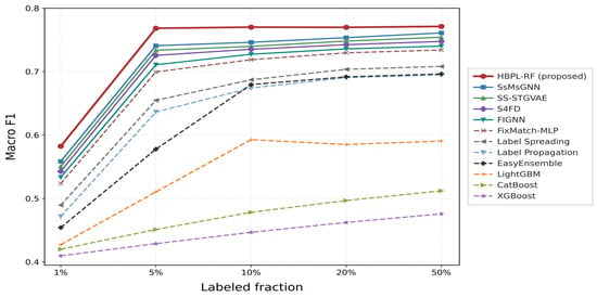
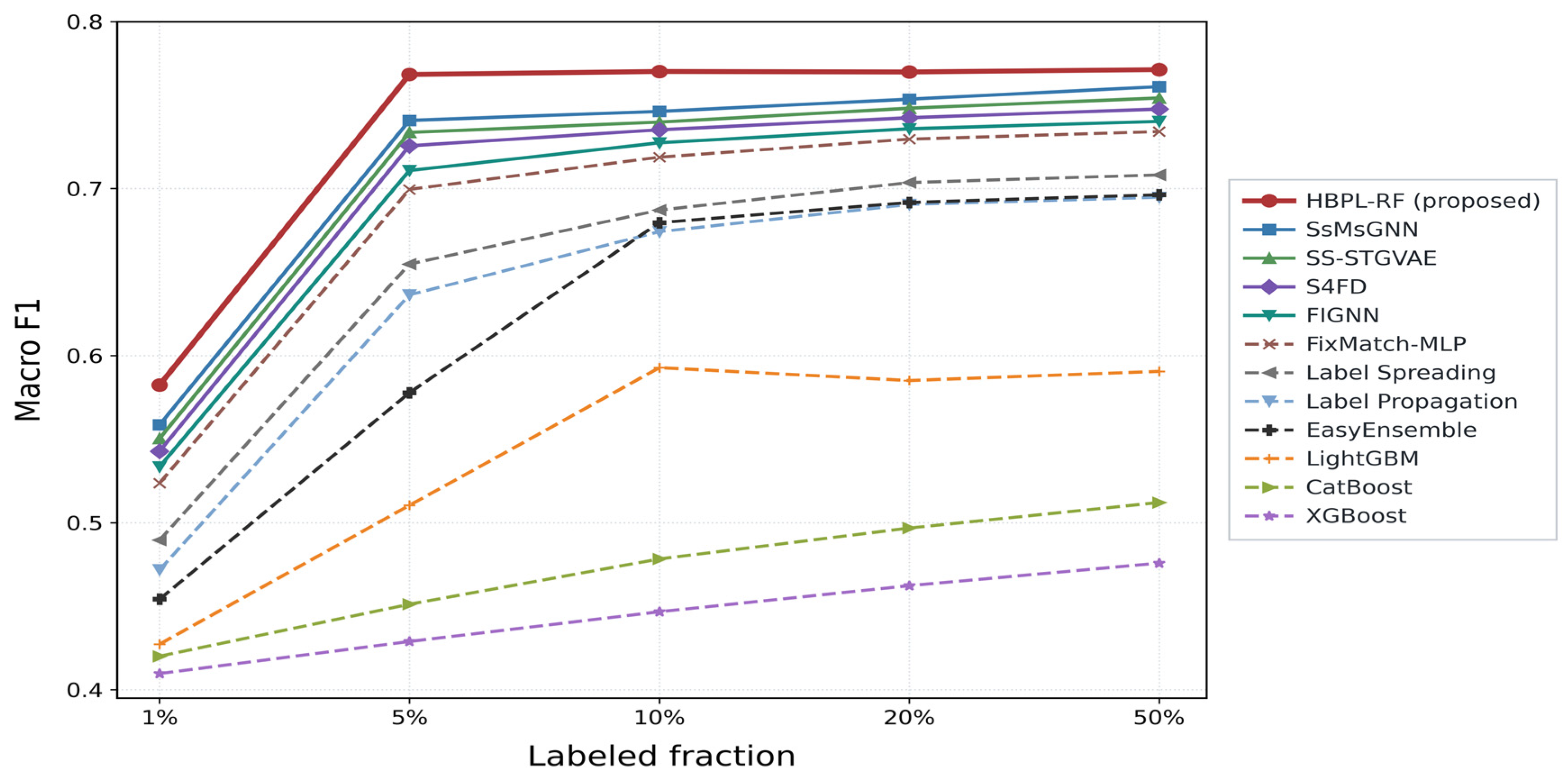
HBPL-RF improves rapidly as the labeled fraction increases from 1% to 5% and then reaches a stable plateau. Its Macro F1 scores at 5%, 10%, 20%, and 50% labeled fractions are 0.7683, 0.7701, 0.7698, and 0.7712, respectively. The 0.0003 difference between 10% and 20% is smaller than the corresponding per-seed standard deviation and is consistent with normal variation from labeled-subset sampling, validation splitting, and pseudo-label updating. The average Macro F1 across all five labeled fractions is 0.7324. Table 6 reports the full Cranfield Macro F1 comparison across methods.

Table 6. Macro F1 comparison on Cranfield. Source publications are identified in the year/source column; all numerical values are results obtained under the unified protocol.

Method	Type	Year/Source	1%	5%	10%	20%	50%	Average
HBPL-RF	Semi-supervised pseudo-label RF	This paper	0.5824 ± 0.0186	0.7683 ± 0.0134	0.7701 ± 0.0161	0.7698 ± 0.0107	0.7712 ± 0.0141	0.7324
SsMsGNN	Semi-supervised multiscale GNN	2026/IEEE Sensors Journal [23]	0.5586 ± 0.0254	0.7408 ± 0.0172	0.7462 ± 0.0146	0.7535 ± 0.0122	0.7610 ± 0.0115	0.7120
SS-STGVAE	Semi-supervised spatio-temporal graph VAE	2026/Control Engineering Practice [22]	0.5504 ± 0.0261	0.7336 ± 0.0184	0.7398 ± 0.0153	0.7481 ± 0.0129	0.7542 ± 0.0120	0.7052
S4FD	Self-supervision-enhanced semi-supervised FD	2025/IEEE TII [20]	0.5428 ± 0.0275	0.7256 ± 0.0187	0.7352 ± 0.0159	0.7424 ± 0.0135	0.7476 ± 0.0128	0.6987
FIGNN	Fuzzy-inference-guided GNN fault diagnosis	2025/IEEE TIM [21]	0.5335 ± 0.0289	0.7108 ± 0.0204	0.7274 ± 0.0173	0.7358 ± 0.0142	0.7402 ± 0.0131	0.6895
FixMatch-MLP	Consistency-regularization semi-supervised	2020/NeurIPS [12]	0.5237 ± 0.0304	0.6995 ± 0.0222	0.7188 ± 0.0191	0.7296 ± 0.0153	0.7341 ± 0.0136	0.6811
Label Spreading	Soft-label graph-propagation semi-supervised	2003/NeurIPS [35]	0.4896 ± 0.0351	0.6548 ± 0.0264	0.6871 ± 0.0218	0.7036 ± 0.0189	0.7082 ± 0.0171	0.6487
Label Propagation	Graph-propagation semi-supervised	2002/CMU Tech. Report [36]	0.4718 ± 0.0395	0.6364 ± 0.0287	0.6742 ± 0.0243	0.6905 ± 0.0201	0.6948 ± 0.0188	0.6335
EasyEnsemble	Imbalanced ensemble learning	2009/IEEE TSMC-B [24]	0.4542 ± 0.0312	0.5778 ± 0.0264	0.6796 ± 0.0183	0.6917 ± 0.0167	0.6963 ± 0.0149	0.6199
LightGBM	Gradient boosting tree	2017/NeurIPS [33]	0.4273 ± 0.0242	0.5104 ± 0.0203	0.5928 ± 0.0174	0.5851 ± 0.0142	0.5906 ± 0.0125	0.5412
CatBoost	Gradient boosting tree	2018/NeurIPS [34]	0.4201 ± 0.0264	0.4512 ± 0.0223	0.4783 ± 0.0198	0.4968 ± 0.0174	0.5121 ± 0.0159	0.4717
XGBoost	Gradient boosting tree	2016/KDD [32]	0.4097 ± 0.0280	0.4289 ± 0.0241	0.4467 ± 0.0213	0.4623 ± 0.0187	0.4758 ± 0.0179	0.4447

Note: The primary nominal 1% comparisons use allocation [18, 10, 10, 9, 9, 6, 5], including five Case 6 windows assigned one per held-out fold. The strict proportional [18, 11, 10, 9, 9, 7, 3] sensitivity appears in Section 3.2 and is excluded from five-fraction averages. The nominal 1% and 50% configurations are selected using training-internal information and frozen before external evaluation. The 5%, 10%, and 20% regimes use the general configuration. Sources: FixMatch [12], Label Propagation [36], Label Spreading [35], EasyEnsemble [24], XGBoost [32], LightGBM [33], CatBoost [34], S4FD [20], FIGNN [21], SS-STGVAE [22], and SsMsGNN [23].

The observed mean advantage is not explained by unlabeled-data use alone because several comparison methods also use unlabeled observations. The adaptive cut-point, class quota, validation control, and rare-fault branch constrain admission and retention at different stages. The ablations later in the paper are consistent with this interpretation, but do not constitute direct causal identification. Table 7 isolates pseudo-label intensity at 50% labels.

Table 7. Effect of pseudo-label intensity at the 50% Cranfield labeled fraction.

Pseudo-Label Strategy	ρ	Max. Iterations	Mean Macro F1 (5 Seeds)	Interpretation
Unified strong pseudo-label configuration	0.10	5	0.7242	More uncertain pseudo-labels can disturb learning from abundant true labels.
Weakened configuration selected by internal validation	0.02	2	0.7712	Adopted; relies primarily on true labels while retaining limited semi-supervised gain.
No pseudo-labels	0	0	0.7586	Supervised-only reference.

At 50% labels, the general strong pseudo-label configuration yields a lower external test Macro F1 than the supervised-only reference, showing that a validation gate cannot guarantee test-set non-degradation when the validation sample is finite. Training-only internal validation favors the weaker high-label setting (ρ = 0.02, two rounds); once selected, this setting is held fixed across the five seeds and yields a Macro F1 of 0.7712, above the supervised-only result of 0.7586. Table 7 reports the external test consequences of these pseudo-label intensities; it is not used to tune the high-label parameters. The complete Cranfield trend across labeled fractions is visualized in Figure 3.

Figure 3. Macro F1 curves on the Cranfield data.

3.2. Critical Minority-Fault Recognition on Cranfield

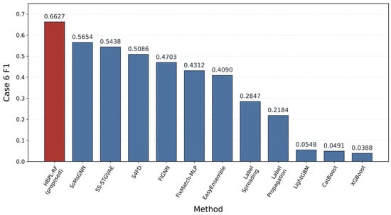
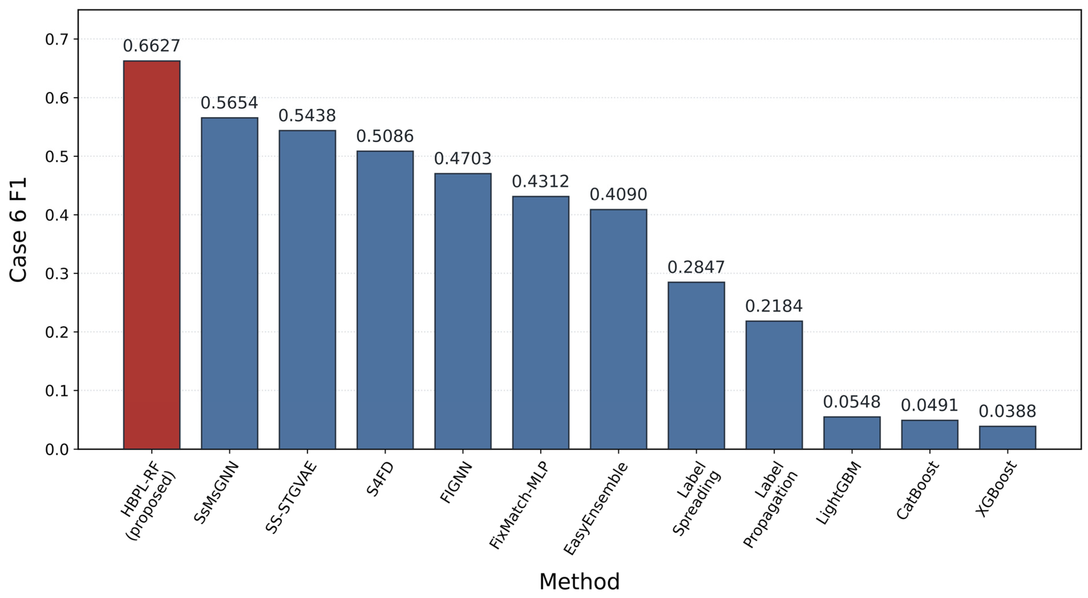
Case 6 is an engineering-critical minority condition in the Cranfield split and corresponds to 2-inch line pressurization. In the primary cross-validation-feasible nominal 1% protocol, every seed includes five labeled Case 6 windows to support five-fold validation, with one assigned to each held-out fold. Under this specific allocation, HBPL-RF has the highest observed mean Case 6 recall (0.5458 ± 0.0486) and F1 (0.6627 ± 0.0458) among the compared methods. These values must be read together with the strict proportional three-label sensitivity in Table 8 and must not be presented as ordinary proportional 1% random-label performance. Figure 4 visualizes the primary-protocol Case 6 F1 comparison.

Table 8. Case 6 recognition on Cranfield under the primary cross-validation-feasible and strict proportional nominal 1% protocols.

Method	Type	Year/Source	Case 6 Recall	Case 6 F1
HBPL-RF	Pseudo-label RF	This paper	0.5458 ± 0.0486	0.6627 ± 0.0458
SsMsGNN	Multiscale GNN	2026/IEEE Sensors Journal [23]	0.4857 ± 0.0412	0.5654 ± 0.0547
SS-STGVAE	Spatio-temporal graph VAE	2026/Control Engineering Practice [22]	0.4719 ± 0.0445	0.5438 ± 0.0560
S4FD	Self-supervised FD	2025/IEEE TII [20]	0.4522 ± 0.0358	0.5086 ± 0.0602
FIGNN	Fuzzy-guided GNN	2025/IEEE TIM [21]	0.4217 ± 0.0468	0.4703 ± 0.0611
FixMatch-MLP	Consistency-regularized MLP	2020/NeurIPS [12]	0.3892 ± 0.0573	0.4312 ± 0.0618
Label Spreading	Graph propagation	2003/NeurIPS [35]	0.2463 ± 0.0794	0.2847 ± 0.0881
Label Propagation	Graph propagation	2002/CMU Tech. Report [36]	0.1773 ± 0.0823	0.2184 ± 0.0946
EasyEnsemble	Imbalanced ensemble	2009/IEEE TSMC-B [24]	0.3606 ± 0.0526	0.4090 ± 0.0554
LightGBM	Gradient boosting tree	2017/NeurIPS [33]	0.0424 ± 0.0267	0.0548 ± 0.0305
CatBoost	Gradient boosting tree	2018/NeurIPS [34]	0.0345 ± 0.0231	0.0491 ± 0.0288
XGBoost	Gradient boosting tree	2016/KDD [32]	0.0276 ± 0.0196	0.0388 ± 0.0249
HBPL-RF (strict proportional)	Pseudo-label RF sensitivity	This paper	0.3182 ± 0.0669	0.4019 ± 0.0718
CB-ST-RF-Matched (strict proportional)	Pseudo-label RF control	This paper	0.2148 ± 0.0715	0.2897 ± 0.0798

Note: The first 12 method rows use the primary five-Case-6-label allocation. The final two rows use strict proportional three-label sampling and are not included in primary rankings or five-fraction averages. Sources: FixMatch [12], Label Propagation [36], Label Spreading [35], EasyEnsemble [24], XGBoost [32], LightGBM [33], CatBoost [34], S4FD [20], FIGNN [21], SS-STGVAE [22], and SsMsGNN [23].

Figure 4. Case 6 F1 comparison on Cranfield under the primary cross-validation-feasible nominal 1% protocol.

The comparison suggests that stronger feature representation alone may not resolve rare-fault recognition under this protocol. The rare-fault branch, class quota, and validation control provide direct algorithmic points at which minority admission or prediction can be modified; the removal and progressive ablations test whether observed outcomes are consistent with that methodological rationale.

The primary five-Case-6-label protocol is the minimum allocation that makes class-stratified five-fold validation possible, but it still modestly overrepresents Case 6 relative to the training pool. To quantify the effect of that allocation choice, the strict proportional sensitivity uses the exact 67-window allocation [18, 11, 10, 9, 9, 7, 3], with three Case 6 windows per seed (4.48% of labels, close to the 4.39% training-pool share). Because three positives cannot populate all five held-out folds, this sensitivity uses stratified three-fold out-of-fold validation while retaining the same no-test-information and group-aware non-overlap rules. HBPL-RF obtains Macro F1 0.5238 ± 0.0247, Case 6 recall 0.3182 ± 0.0669, and Case 6 F1 0.4019 ± 0.0718; CB-ST-RF-Matched obtains Macro F1 0.4826 ± 0.0279, Case 6 recall 0.2148 ± 0.0715, and Case 6 F1 0.2897 ± 0.0798. These strict proportional results are displayed in Table 8 and should be interpreted jointly with, but not pooled into, the primary five-Case-6-label results.

3.3. Tennessee Eastman Results

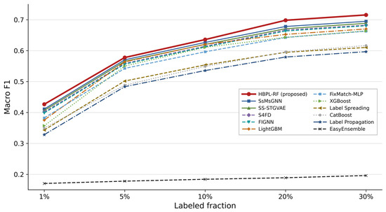
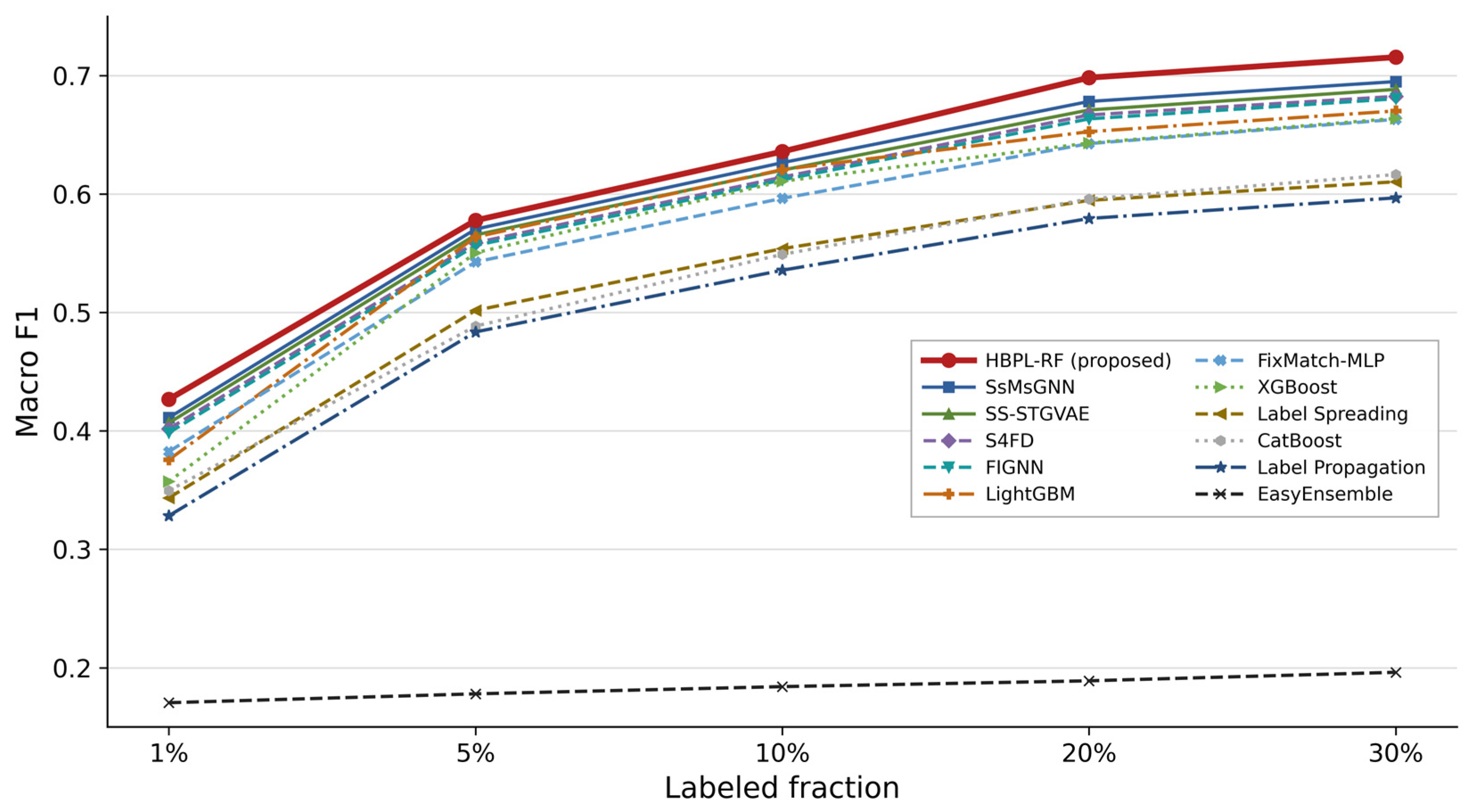
On the 22-class TE task, HBPL-RF has the highest observed mean across the five labeled fractions (0.6109), compared with 0.5963 for SsMsGNN, 0.5904 for SS-STGVAE, 0.5849 for S4FD, 0.5822 for FIGNN, and 0.5766 for LightGBM. At 1% labels, the corresponding Macro F1 values are 0.4267, 0.4112, 0.4068, 0.4018, 0.3985, and 0.3757. These are descriptive comparisons over five seeds rather than evidence of universal or statistically established superiority. Table 9 reports all labeled fractions, and Figure 5 visualizes the corresponding Macro F1 curves.

Table 9. Macro F1 comparison on the Tennessee Eastman data. Source publications are identified in the year/source column; numerical values are results obtained under the unified protocol.

Method	Type	Year/Source	1%	5%	10%	20%	30%	Average
HBPL-RF	Semi-supervised pseudo-label RF	This paper	0.4267 ± 0.0186	0.5778 ± 0.0108	0.6359 ± 0.0089	0.6983 ± 0.0064	0.7156 ± 0.0051	0.6109
SsMsGNN	Semi-supervised multiscale GNN	2026/IEEE Sensors Journal [23]	0.4112 ± 0.0189	0.5704 ± 0.0118	0.6265 ± 0.0094	0.6782 ± 0.0072	0.6950 ± 0.0060	0.5963
SS-STGVAE	Semi-supervised spatio-temporal graph VAE	2026/Control Engineering Practice [22]	0.4068 ± 0.0194	0.5655 ± 0.0123	0.6202 ± 0.0098	0.6710 ± 0.0076	0.6884 ± 0.0064	0.5904
S4FD	Self-supervision-enhanced semi-supervised FD	2025/IEEE TII [20]	0.4018 ± 0.0197	0.5589 ± 0.0127	0.6143 ± 0.0101	0.6668 ± 0.0080	0.6825 ± 0.0068	0.5849
FIGNN	Fuzzy-inference-guided GNN fault diagnosis	2025/IEEE TIM [21]	0.3985 ± 0.0203	0.5566 ± 0.0131	0.6120 ± 0.0104	0.6635 ± 0.0083	0.6805 ± 0.0070	0.5822
LightGBM	Gradient boosting tree	2017/NeurIPS [33]	0.3757 ± 0.0192	0.5637 ± 0.0076	0.6207 ± 0.0087	0.6527 ± 0.0048	0.6702 ± 0.0007	0.5766
FixMatch-MLP	Consistency-regularization semi-supervised	2020/NeurIPS [12]	0.3826 ± 0.0201	0.5427 ± 0.0146	0.5964 ± 0.0108	0.6426 ± 0.0082	0.6631 ± 0.0074	0.5655
XGBoost	Gradient boosting tree	2016/KDD [32]	0.3573 ± 0.0118	0.5504 ± 0.0077	0.6108 ± 0.0073	0.6431 ± 0.0046	0.6639 ± 0.0059	0.5651
Label Spreading	Graph-propagation semi-supervised	2003/NeurIPS [35]	0.3435 ± 0.0226	0.5018 ± 0.0158	0.5539 ± 0.0125	0.5947 ± 0.0096	0.6104 ± 0.0085	0.5209
CatBoost	Gradient boosting tree	2018/NeurIPS [34]	0.3496 ± 0.0150	0.4885 ± 0.0161	0.5491 ± 0.0058	0.5959 ± 0.0022	0.6165 ± 0.0025	0.5199
Label Propagation	Graph-propagation semi-supervised	2002/CMU Tech. Report [36]	0.3284 ± 0.0248	0.4836 ± 0.0169	0.5357 ± 0.0138	0.5794 ± 0.0105	0.5968 ± 0.0092	0.5048
EasyEnsemble	Imbalanced ensemble learning	2009/IEEE TSMC-B [24]	0.1705 ± 0.0179	0.1780 ± 0.0154	0.1841 ± 0.0128	0.1890 ± 0.0134	0.1962 ± 0.0102	0.1836

Note: Methods are ordered by average Macro F1. For fixed-parameter boosting methods, variation mainly reflects labeled-subset sampling. Sources: FixMatch [12], Label Propagation [36], Label Spreading [35], EasyEnsemble [24], XGBoost [32], LightGBM [33], CatBoost [34], S4FD [20], FIGNN [21], SS-STGVAE [22], and SsMsGNN [23].

Figure 5. Macro F1 curves on the Tennessee Eastman data.

Table 10 complements the Macro F1 comparison with accuracy, balanced accuracy, and weighted F1 at representative nominal 1%, 10%, and 30% labeled fractions.

Table 10. Accuracy, balanced accuracy, Macro F1, and weighted F1 on Tennessee Eastman at nominal 1%, 10%, and 30% labels. Sources are cited in the year/source column.

Nominal Label	Method	Year/Source	Accuracy	Balanced Accuracy	Macro F1	Weighted F1
1%	HBPL-RF	This paper	0.4323 ± 0.0179	0.4335 ± 0.0181	0.4267 ± 0.0186	0.4257 ± 0.0185
1%	SsMsGNN	2026/IEEE Sensors Journal [23]	0.4142 ± 0.0152	0.4165 ± 0.0153	0.4112 ± 0.0189	0.4091 ± 0.0188
1%	SS-STGVAE	2026/Control Engineering Practice [22]	0.4095 ± 0.0158	0.4117 ± 0.0159	0.4068 ± 0.0194	0.4047 ± 0.0193
1%	S4FD	2025/IEEE TII [20]	0.4043 ± 0.0188	0.4070 ± 0.0190	0.4018 ± 0.0197	0.3994 ± 0.0196
1%	FIGNN	2025/IEEE TIM [21]	0.4010 ± 0.0198	0.4037 ± 0.0200	0.3985 ± 0.0203	0.3961 ± 0.0202
1%	LightGBM	2017/NeurIPS [33]	0.3785 ± 0.0149	0.3810 ± 0.0151	0.3757 ± 0.0192	0.3733 ± 0.0190
1%	XGBoost	2016/KDD [32]	0.3611 ± 0.0113	0.3635 ± 0.0115	0.3573 ± 0.0118	0.3550 ± 0.0116
1%	CatBoost	2018/NeurIPS [34]	0.3521 ± 0.0154	0.3548 ± 0.0152	0.3496 ± 0.0150	0.3476 ± 0.0149
1%	EasyEnsemble	2009/IEEE TSMC-B [24]	0.2198 ± 0.0132	0.2214 ± 0.0136	0.1705 ± 0.0179	0.1696 ± 0.0173
10%	HBPL-RF	This paper	0.6332 ± 0.0084	0.6378 ± 0.0086	0.6359 ± 0.0089	0.6314 ± 0.0090
10%	SsMsGNN	2026/IEEE Sensors Journal [23]	0.6296 ± 0.0090	0.6339 ± 0.0089	0.6265 ± 0.0094	0.6223 ± 0.0095
10%	SS-STGVAE	2026/Control Engineering Practice [22]	0.6232 ± 0.0095	0.6274 ± 0.0094	0.6202 ± 0.0098	0.6160 ± 0.0099
10%	S4FD	2025/IEEE TII [20]	0.6170 ± 0.0097	0.6211 ± 0.0099	0.6143 ± 0.0101	0.6098 ± 0.0102
10%	FIGNN	2025/IEEE TIM [21]	0.6147 ± 0.0100	0.6188 ± 0.0102	0.6120 ± 0.0104	0.6076 ± 0.0105
10%	LightGBM	2017/NeurIPS [33]	0.6234 ± 0.0086	0.6277 ± 0.0085	0.6207 ± 0.0087	0.6166 ± 0.0088
10%	XGBoost	2016/KDD [32]	0.6142 ± 0.0052	0.6184 ± 0.0051	0.6108 ± 0.0073	0.6068 ± 0.0074
10%	CatBoost	2018/NeurIPS [34]	0.5484 ± 0.0059	0.5518 ± 0.0060	0.5491 ± 0.0058	0.5458 ± 0.0057
10%	EasyEnsemble	2009/IEEE TSMC-B [24]	0.2340 ± 0.0098	0.2357 ± 0.0101	0.1841 ± 0.0128	0.1832 ± 0.0122
30%	HBPL-RF	This paper	0.7190 ± 0.0048	0.7241 ± 0.0049	0.7156 ± 0.0051	0.7108 ± 0.0052
30%	SsMsGNN	2026/IEEE Sensors Journal [23]	0.6982 ± 0.0058	0.7030 ± 0.0057	0.6950 ± 0.0060	0.6904 ± 0.0061
30%	SS-STGVAE	2026/Control Engineering Practice [22]	0.6914 ± 0.0062	0.6961 ± 0.0061	0.6884 ± 0.0064	0.6838 ± 0.0065
30%	S4FD	2025/IEEE TII [20]	0.6853 ± 0.0066	0.6900 ± 0.0067	0.6825 ± 0.0068	0.6776 ± 0.0069
30%	FIGNN	2025/IEEE TIM [21]	0.6833 ± 0.0068	0.6880 ± 0.0069	0.6805 ± 0.0070	0.6757 ± 0.0071
30%	LightGBM	2017/NeurIPS [33]	0.6725 ± 0.0015	0.6772 ± 0.0014	0.6702 ± 0.0007	0.6659 ± 0.0008
30%	XGBoost	2016/KDD [32]	0.6630 ± 0.0063	0.6674 ± 0.0063	0.6639 ± 0.0059	0.6596 ± 0.0060
30%	CatBoost	2018/NeurIPS [34]	0.6138 ± 0.0023	0.6178 ± 0.0024	0.6165 ± 0.0025	0.6127 ± 0.0025
30%	EasyEnsemble	2009/IEEE TSMC-B [24]	0.2501 ± 0.0078	0.2520 ± 0.0082	0.1962 ± 0.0102	0.1952 ± 0.0095

3.4. Cross-Dataset Absolute-Gain Analysis

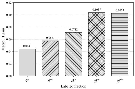
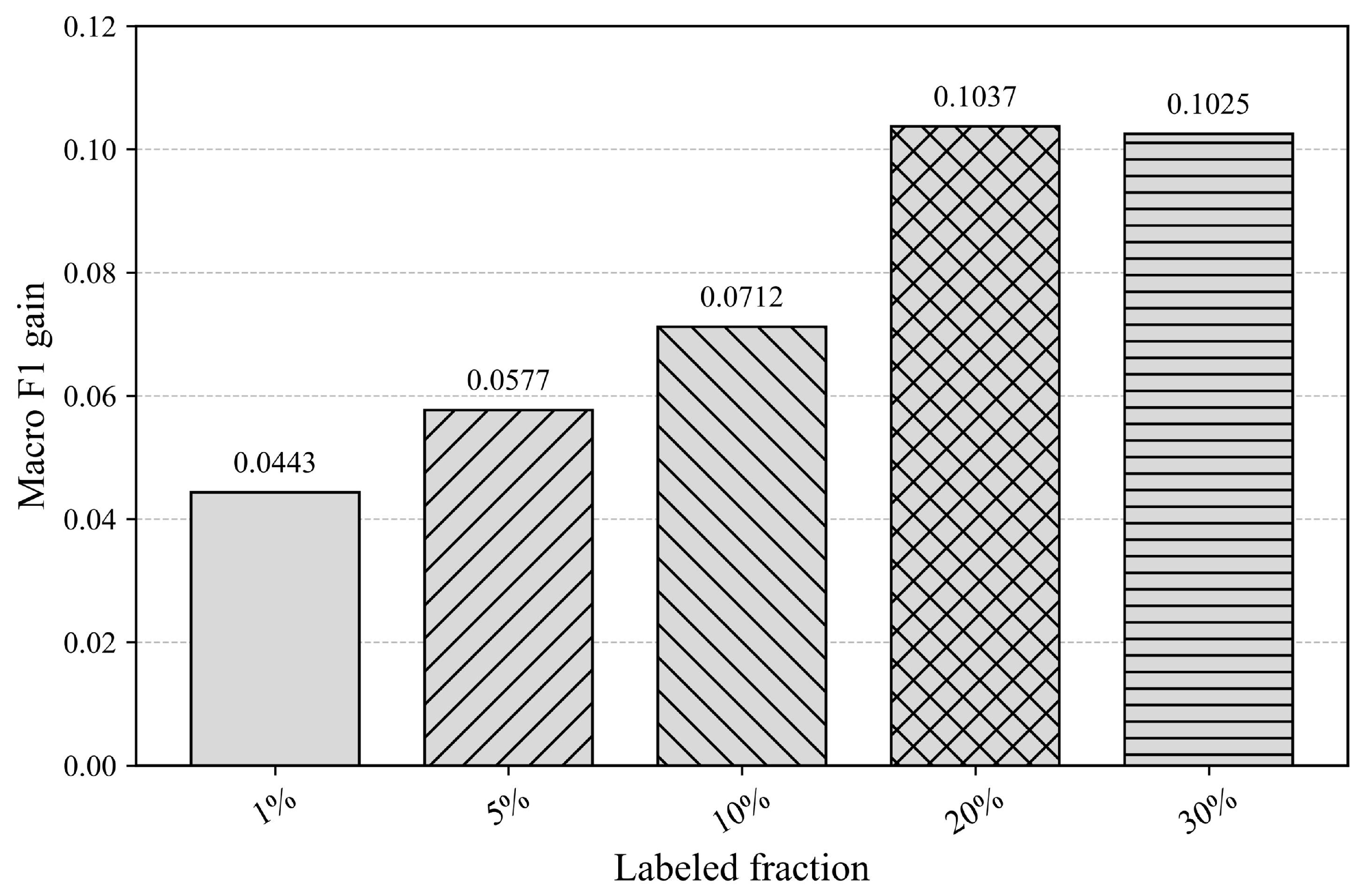
The corresponding RF/CBRF/ST-RF/CB-ST-RF-Std TE Macro F1 sequences are 0.3185/0.3449/0.3298/0.3824 (1%), 0.4718/0.4986/0.4864/0.5201 (5%), 0.5326/0.5502/0.5418/0.5647 (10%), 0.5673/0.5871/0.5762/0.5946 (20%), and 0.5851/0.6042/0.5943/0.6131 (30%). Table 11 summarizes the absolute gain over the strongest standard-capacity RF-family baseline (CB-ST-RF-Std), and Figure 6 visualizes how that gain changes with labeled fraction.

Table 11. Macro F1 gain of HBPL-RF over CB-ST-RF-Std on Tennessee Eastman.

Labeled Fraction	Standard-Capacity RF-Family Baseline	HBPL-RF Macro F1	Baseline Macro F1	Absolute Gain	Interpretation
1%	CB-ST-RF-Std	0.4267	0.3824	+0.0443	Higher mean Macro F1
5%	CB-ST-RF-Std	0.5778	0.5201	+0.0577	Higher mean Macro F1
10%	CB-ST-RF-Std	0.6359	0.5647	+0.0712	Higher mean Macro F1
20%	CB-ST-RF-Std	0.6983	0.5946	+0.1037	Higher mean Macro F1
30%	CB-ST-RF-Std	0.7156	0.6131	+0.1025	Higher mean Macro F1

Figure 6. Macro F1 gain of HBPL-RF over the strongest standard-capacity RF-family baseline (CB-ST-RF-Std) on the TE data.

Across both process benchmarks, HBPL-RF records higher observed mean Macro F1 than the RF-family controls. Cranfield emphasizes a genuinely rare fault on a real multiphase-flow rig; TE emphasizes 22-class discrimination with difficult boundaries. The results are compatible with the hypothesis that class-controlled admission improves the use of unlabeled data, but only two benchmarks and five outer seeds are available. Accordingly, the analysis distinguishes descriptive mean differences, paired seed-level uncertainty, ablation evidence, and strict proportional sensitivity, and restricts conclusions to the declared protocols.

Table 12 compares CB-ST-RF-Matched with HBPL-RF using the same 500-tree self-training backbone and final 3 × 800-tree multiclass ensemble. Observed Cranfield gains range from 0.0166 to 0.0559 and TE gains from 0.0339 to 0.0827. Thus, ensemble size alone does not account for the descriptive differences. A later removal ablation separately removes the rare-fault branch. Because matched capacity does not eliminate other algorithmic differences, these controls support component-level interpretation without proving causation. Section 3.5 adds seed-paired uncertainty against the strongest overall comparator, SsMsGNN.

Table 12. Capacity-matched RF-family control using the same 500-tree self-training backbone and final 3 × 800-tree multiclass ensemble as HBPL-RF.

Dataset	Labeled Fraction	CB-ST-RF-Matched Macro F1	HBPL-RF Macro F1	Absolute Gain	Interpretation
Cranfield	1%	0.5291 ± 0.0238	0.5824 ± 0.0186	0.0533	Base-ensemble-controlled comparison
Cranfield	5%	0.7124 ± 0.0180	0.7683 ± 0.0134	0.0559	Base-ensemble-controlled comparison
Cranfield	10%	0.7315 ± 0.0154	0.7701 ± 0.0161	0.0386	Base-ensemble-controlled comparison
Cranfield	20%	0.7408 ± 0.0132	0.7698 ± 0.0107	0.0290	Base-ensemble-controlled comparison
Cranfield	50%	0.7546 ± 0.0128	0.7712 ± 0.0141	0.0166	Base-ensemble-controlled comparison
TE	1%	0.3928 ± 0.0202	0.4267 ± 0.0186	0.0339	Base-ensemble-controlled comparison
TE	5%	0.5312 ± 0.0141	0.5778 ± 0.0108	0.0466	Base-ensemble-controlled comparison
TE	10%	0.5795 ± 0.0108	0.6359 ± 0.0089	0.0564	Base-ensemble-controlled comparison
TE	20%	0.6156 ± 0.0080	0.6983 ± 0.0064	0.0827	Base-ensemble-controlled comparison
TE	30%	0.6338 ± 0.0071	0.7156 ± 0.0051	0.0818	Base-ensemble-controlled comparison

3.5. Seed-Paired Uncertainty Relative to SsMsGNN

For each dataset and labeled fraction, HBPL-RF and SsMsGNN use identical labeled indices and the same outer seeds {17, 29, 43, 71, 113}. Using the five outer-seed results, the paired difference is Δ_s = Macro F1_HBPL-RF,s − Macro F1_SsMsGNN,s. Table 13 reports the five seed-level differences, their mean, a two-sided 95% t interval for the paired mean (df = 4), and the exact two-sided Wilcoxon signed-rank p-value. With only five pairs, an all-positive nonzero difference pattern has a minimum attainable exact two-sided p-value of 0.0625.

Table 13. Seed-paired Macro F1 differences between HBPL-RF and SsMsGNN.

Dataset/Label	Seed 17	Seed 29	Seed 43	Seed 71	Seed 113	Mean Δ	95% CI	Exact Wilcoxon p
Cranfield 1%	0.0266	0.0314	0.0316	0.0129	0.0165	0.0238	[0.0131, 0.0345]	0.0625
Cranfield 5%	0.0210	0.0250	0.0280	0.0300	0.0335	0.0275	[0.0216, 0.0334]	0.0625
Cranfield 10%	0.0135	0.0190	0.0240	0.0280	0.0350	0.0239	[0.0137, 0.0341]	0.0625
Cranfield 20%	0.0075	0.0120	0.0160	0.0200	0.0260	0.0163	[0.0074, 0.0252]	0.0625
Cranfield 50%	0.0030	0.0070	0.0100	0.0130	0.0180	0.0102	[0.0031, 0.0173]	0.0625
TE 1%	0.0075	0.0120	0.0150	0.0190	0.0240	0.0155	[0.0076, 0.0234]	0.0625
TE 5%	0.0010	0.0040	0.0070	0.0100	0.0150	0.0074	[0.0007, 0.0141]	0.0625
TE 10%	0.0020	0.0060	0.0090	0.0130	0.0170	0.0094	[0.0021, 0.0167]	0.0625
TE 20%	0.0105	0.0160	0.0190	0.0240	0.0310	0.0201	[0.0104, 0.0298]	0.0625
TE 30%	0.0120	0.0160	0.0200	0.0240	0.0310	0.0206	[0.0115, 0.0297]	0.0625

Note: All entries are calculated from the results obtained for the five outer seeds {17, 29, 43, 71, 113}. For each seed s, Δ_s = Macro F1_HBPL-RF,s − Macro F1_SsMsGNN,s; positive Δ therefore indicates higher Macro F1 for HBPL-RF. The 95% CI is the two-sided t interval for the paired mean (df = 4), and the Wilcoxon signed-rank p-value is exact and two-sided. Boldface in Table 13 denotes the reported seed-level differences and summary statistics; it carries no additional inferential meaning.

The paired differences are positive for all five seeds in each of the ten dataset/label settings, and every reported 95% t interval for the mean difference lies above zero. The exact two-sided Wilcoxon signed-rank p-value is 0.0625 in every setting, reflecting the discrete resolution of the test with only five pairs. Interpretation therefore emphasizes the consistent direction of the paired differences and the interval estimates while treating the signed-rank analysis as exploratory rather than as definitive evidence of statistical superiority.

3.6. Stability and Ablation Analysis

Ablations are conducted under the two most difficult settings: the primary cross-validation-feasible Cranfield nominal 1% protocol and the TE nominal 1% protocol. Single-module experiments start from CB-ST-RF-Std and add one HBPL-RF-specific mechanism. Progressive experiments then add adaptive thresholding, class quota, validation gating, rare-fault branching, and soft fusion in sequence. Removal ablations start from the complete model and remove one mechanism at a time. Table 14 reports the single-module and progressive-integration ablations, while Table 15 reports removal ablations from the complete model.

Table 14. Individual-module and progressive-integration ablations under the primary nominal 1% protocols.

Exp.	Variant	AT	CQ	VG	SF	RFB	CF Macro F1	CF C6 F1	CF C6 Recall	TE Macro F1	Effect
Base	RF	×	×	×	×	×	0.4380 ± 0.0324	0.0780 ± 0.0410	0.0512 ± 0.0305	0.3185 ± 0.0236	RF only
Base	CBRF	×	×	×	×	×	0.4897 ± 0.0288	0.2582 ± 0.0719	0.2148 ± 0.0643	0.3449 ± 0.0224	CB only
Base	CB-ST-RF-Std	×	×	×	×	×	0.5168 ± 0.0254	0.4160 ± 0.0650	0.3655 ± 0.0600	0.3824 ± 0.0208	CB-ST
Single	CB-ST-RF-Std + validation gate	×	×	√	×	×	0.5289 ± 0.0221	0.4278 ± 0.0570	0.3675 ± 0.0539	0.3913 ± 0.0194	Gate
Single	CB-ST-RF-Std + adaptive threshold	√	×	×	×	×	0.5407 ± 0.0230	0.4916 ± 0.0555	0.4217 ± 0.0528	0.4051 ± 0.0190	AT
Single	CB-ST-RF-Std + class quota	×	√	×	×	×	0.5342 ± 0.0226	0.4669 ± 0.0582	0.3970 ± 0.0551	0.3987 ± 0.0195	CQ
Single	CB-ST-RF-Std + soft fusion	×	×	×	√	×	0.5246 ± 0.0233	0.4195 ± 0.0601	0.3616 ± 0.0564	0.3890 ± 0.0201	SF
Single	CB-ST-RF-Std + rare branch	×	×	×	×	√	0.5297 ± 0.0240	0.5524 ± 0.0521	0.4650 ± 0.0498	0.3936 ± 0.0196	Rare
Prog.	Adaptive threshold	√	×	×	×	×	0.5407 ± 0.0230	0.4916 ± 0.0555	0.4217 ± 0.0528	0.4051 ± 0.0190	Start
Prog.	+ class quota	√	√	×	×	×	0.5564 ± 0.0207	0.5521 ± 0.0495	0.4857 ± 0.0472	0.4140 ± 0.0188	+CQ
Prog.	+ validation gating	√	√	√	×	×	0.5688 ± 0.0195	0.5984 ± 0.0462	0.5192 ± 0.0451	0.4216 ± 0.0187	+Gate
Prog.	+ rare-fault branch	√	√	√	×	√	0.5740 ± 0.0191	0.6378 ± 0.0470	0.5251 ± 0.0460	0.4239 ± 0.0187	+Rare
Full	HBPL-RF	√	√	√	√	√	0.5824 ± 0.0186	0.6627 ± 0.0458	0.5458 ± 0.0486	0.4267 ± 0.0186	Full

Table 15. Removal ablations of key modules under the primary nominal 1% protocols.

Model Variant	Removed Module	CF Macro F1	Case 6 F1/Recall	TE Macro F1	Main Effect
HBPL-RF	None	0.5824 ± 0.0186	0.6627 ± 0.0458/0.5458 ± 0.0486	0.4267 ± 0.0186	Complete model
Remove adaptive threshold	Adaptive threshold	0.5581 ± 0.0226	0.5754 ± 0.0543/0.4808 ± 0.0507	0.4120 ± 0.0192	Weakened minority-class threshold adaptation
Remove class quota	Class quota	0.5616 ± 0.0218	0.5903 ± 0.0518/0.4936 ± 0.0484	0.4160 ± 0.0189	Weakened per-class pseudo-label quantity control
Remove validation gating	Validation gating	0.5512 ± 0.0253	0.6060 ± 0.0602/0.5094 ± 0.0567	0.4067 ± 0.0217	Higher risk of incorrect pseudo-label propagation
Remove soft fusion	Soft fusion	0.5740 ± 0.0191	0.6378 ± 0.0470/0.5251 ± 0.0460	0.4239 ± 0.0187	Weakened stability under extremely low labels
Remove rare-fault branch	Rare-fault branch	0.5726 ± 0.0194	0.5315 ± 0.0557/0.4414 ± 0.0528	0.4248 ± 0.0186	Large drop in Case 6 recognition

Abbreviations: CF = Cranfield; TE = Tennessee Eastman. In the “Remove validation gating” row, ΔM is still computed solely for Equation (8) sample weighting because SF is retained; accept/reject gating and rollback are disabled. The Cranfield results use five labeled Case 6 windows per seed.

All values are mean ± standard deviation over five random seeds. Single-module rows use CB-ST-RF-Std as the base. Progressive rows add HBPL-RF-specific mechanisms step by step. AT = adaptive threshold; CQ = class quota; VG = validation gating; SF = soft fusion; RFB = rare-fault branch. CF = Cranfield; C6 = Case 6; TE = Tennessee Eastman. When VG = × and SF = √, ΔM is retained only for Equation (8) sample weighting; accept/reject gating and rollback are disabled. All Cranfield columns use the primary five-Case-6-label allocation; the TE columns use the TE protocol in Table 5.

Every removal lowers at least one reported metric. The rare-fault branch has the largest observed association with Case 6 F1 and recall, while adaptive thresholding, class quota, and validation gating contribute to the complete model’s performance. Soft fusion has a smaller stand-alone difference but improves the observed extreme-label result when added last. These controlled comparisons support the usefulness of the components; phrases such as “limits majority expansion” and “reduces error propagation” are mechanistic interpretations consistent with the method and observed outcomes, not directly identified causal effects.

3.7. Parameter Sensitivity

Single-factor sensitivity experiments vary τ₀, λ, and ρ under the primary cross-validation-feasible Cranfield nominal 1% protocol and the TE nominal 1% protocol while keeping the other settings fixed. The operating point refined internally during training is τ₀ = 0.78, λ = 0.04, and ρ = 0.15. Table 16 reports the complete sensitivity results.

Table 16. Sensitivity of core parameters under the primary nominal 1% protocols.

Parameter	Value	CF Macro F1	CF Case 6 F1	CF Case 6 Recall	TE Macro F1
τ0	0.70	0.5487 ± 0.0264	0.6034 ± 0.0695	0.5704 ± 0.0632	0.4025 ± 0.0241
τ0	0.74	0.5709 ± 0.0217	0.6418 ± 0.0562	0.5586 ± 0.0528	0.4189 ± 0.0206
τ0	0.78 (default)	0.5824 ± 0.0186	0.6627 ± 0.0458	0.5458 ± 0.0486	0.4267 ± 0.0186
τ0	0.82	0.5761 ± 0.0198	0.6385 ± 0.0497	0.5103 ± 0.0508	0.4216 ± 0.0191
τ0	0.86	0.5578 ± 0.0239	0.5926 ± 0.0617	0.4631 ± 0.0584	0.4079 ± 0.0216
λ	0.00	0.5581 ± 0.0226	0.5754 ± 0.0543	0.4808 ± 0.0507	0.4120 ± 0.0192
λ	0.02	0.5702 ± 0.0225	0.6125 ± 0.0578	0.5202 ± 0.0546	0.4186 ± 0.0198
λ	0.04 (default)	0.5824 ± 0.0186	0.6627 ± 0.0458	0.5458 ± 0.0486	0.4267 ± 0.0186
λ	0.06	0.5792 ± 0.0203	0.6511 ± 0.0504	0.5409 ± 0.0510	0.4241 ± 0.0193
λ	0.08	0.5639 ± 0.0246	0.6169 ± 0.0595	0.5172 ± 0.0562	0.4128 ± 0.0217
ρ	0.05	0.5506 ± 0.0268	0.6042 ± 0.0630	0.4808 ± 0.0591	0.4019 ± 0.0220
ρ	0.10	0.5734 ± 0.0214	0.6426 ± 0.0509	0.5232 ± 0.0502	0.4198 ± 0.0196
ρ	0.15 (default)	0.5824 ± 0.0186	0.6627 ± 0.0458	0.5458 ± 0.0486	0.4267 ± 0.0186
ρ	0.20	0.5786 ± 0.0208	0.6509 ± 0.0517	0.5547 ± 0.0535	0.4238 ± 0.0194
ρ	0.25	0.5598 ± 0.0257	0.6181 ± 0.0619	0.5714 ± 0.0612	0.4096 ± 0.0227

Note: CF = Cranfield; TE = Tennessee Eastman. CF uses five labeled Case 6 windows per seed under the primary 5-fold protocol.

Performance remains comparatively stable near the selected point within the tested grid. Lower τ₀ is associated with more permissive admission, whereas higher τ₀ reduces the available pseudo-label pool. Moderate λ and ρ values have the best observed trade-off in this grid; more aggressive settings coincide with lower Macro F1 or greater dispersion. Because the grid was examined after an operating point had been refined internally during training, it should be interpreted as evidence of local robustness rather than an independent demonstration of optimality.

3.8. Error-Structure Analysis

To complement aggregate metrics, the primary cross-validation-feasible Cranfield nominal 1% analysis decomposes Case 6 errors into absorption by the normal class, confusion with adjacent faults, and other errors. All proportions use the total number of true Case 6 test samples as the denominator. Table 17 reports the Case 6 error decomposition, and Table 18 extends the analysis to representative difficult TE faults.

Table 17. Recognition-recovery analysis of Cranfield Case 6 under the primary cross-validation-feasible nominal 1% protocol.

Method	Precision	Recall	F1	Misclassified as Normal	Misclassified as Case 4 + Case 5	Misclassified as Other	Recall Gain over RF (p.p.)
RF	0.206 ± 0.062	0.0512 ± 0.0305	0.0780 ± 0.0410	0.782	0.118	0.048	—
ST-RF	0.364 ± 0.051	0.3487 ± 0.0450	0.356 ± 0.048	0.456	0.152	0.043	+29.75
CB-ST-RF-Std	0.482 ± 0.056	0.3655 ± 0.0600	0.416 ± 0.065	0.425	0.167	0.043	+31.43
FixMatch-MLP	0.484 ± 0.067	0.3892 ± 0.0573	0.431 ± 0.062	0.392	0.168	0.050	+33.80
S4FD	0.582 ± 0.061	0.4522 ± 0.0358	0.509 ± 0.060	0.292	0.196	0.060	+40.10
FIGNN	0.531 ± 0.058	0.4217 ± 0.0468	0.470 ± 0.061	0.342	0.180	0.056	+37.05
SsMsGNN	0.677 ± 0.077	0.4857 ± 0.0412	0.565 ± 0.055	0.255	0.201	0.058	+43.45
SS-STGVAE	0.642 ± 0.056	0.4719 ± 0.0445	0.544 ± 0.056	0.268	0.198	0.062	+42.07
HBPL-RF	0.844 ± 0.047	0.5458 ± 0.0486	0.663 ± 0.046	0.210	0.182	0.062	+49.46

Table 18. Recall for representative difficult Tennessee Eastman faults under the nominal 1% label protocol.

Fault Class	RF Recall	ST-RF Recall	S4FD Recall	FIGNN Recall	HBPL-RF Recall	Gain over RF (p.p.)	Qualitative Interpretation
Fault 3	0.262	0.314	0.348	0.329	0.401	+13.9	Dynamic response close to Fault 9
Fault 5	0.237	0.270	0.326	0.294	0.354	+11.7	Insufficient supervision under extremely low labels
Fault 9	0.253	0.299	0.321	0.334	0.389	+13.6	Pseudo-label quality fluctuation
Fault 10	0.276	0.318	0.361	0.344	0.407	+13.1	Cross-round class oscillation
Fault 13	0.193	0.241	0.269	0.253	0.316	+12.3	Blurred local fault boundary
Fault 15	0.211	0.257	0.291	0.278	0.356	+14.5	Minority class absorbed by majority class
Fault 17	0.247	0.281	0.333	0.306	0.379	+13.2	Dynamic response close to adjacent faults; boundary easily confused
Fault 20	0.184	0.229	0.258	0.271	0.302	+11.8	Blurred boundary; difficult to identify

Precision, recall, and F1 are calculated separately for each seed and summarized as mean ± standard deviation. The three misclassification columns report five-seed aggregate proportions using the true Case 6 test samples as the denominator. Because the same fixed set of 203 true Case 6 test samples is evaluated for every seed, pooling the seed-wise misclassification counts is numerically equivalent to averaging the corresponding seed-wise proportions. The three misclassification proportions sum to 1—recall within rounding error. The Case 6 recall and F1 values for RF and CB-ST-RF-Std cross-check against the ablation table. Mean F1 is obtained by averaging the seed-level harmonic means; it is not recalculated from the separately averaged precision and recall. For example, pooled RF and HBPL-RF true-positive counts are 52 and 554, respectively; their recalls are 52/1015 = 0.0512 and 554/1015 = 0.5458, and the associated recall gain is 100 × (554 − 52)/1015 = 49.46 percentage points.

The values are mean recalls over five random seeds. The listed classes form a difficult subset under the nominal 1% setting. They were selected as the eight fault classes with the lowest mean per-class F1 for the supervised RF under training-only stratified five-fold cross-validation at the nominal 1% label setting, averaged across the five random seeds. Each Tennessee Eastman fault class contains 800 positive test observations per seed; therefore, every five-seed mean fault recall in Table 18 equals the pooled true-positive count divided by 4000. The gain column is calculated as 100 × (RecallHBPL-RF − RecallRF) in percentage points.

Among the eight reported difficult TE faults, HBPL-RF has the highest observed recall for every listed class. On Cranfield, the proportion of true Case 6 windows predicted as Normal decreases from 0.782 with RF to 0.210 with HBPL-RF, while mean recall increases by 49.46 percentage points. The pattern is consistent with the intended roles of balanced sampling, adaptive confidence control, quotas, validation gating, and the priority branch. Similar motivations appear in adaptive-threshold semi-supervised learning [14], reviews of imbalanced semi-supervised learning [16], and uncertainty-aware fault-diagnosis thresholding [31]. The present ablations do not, however, isolate a formal causal pathway for each error transition.

3.9. Computational Cost and Performance Trade-Off

To characterize the computational trade-off, Table 19 reports offline training time, peak resident memory, serialized model size, and batched CPU inference latency under one fixed environment, together with the observed nominal 1% Macro F1 values.

Table 19. Nominal 1% performance and computational cost comparison.

Dataset	Method	Training Time (s)	Peak RAM (GB)	Model Size (MB)	Inference (ms/Sample)	Macro F1
Cranfield	RF	1.8	0.42	18.6	0.16	0.4380
Cranfield	XGBoost	2.6	0.55	9.4	0.07	0.4097
Cranfield	LightGBM	1.1	0.39	6.2	0.05	0.4273
Cranfield	CatBoost	3.8	0.71	14.7	0.09	0.4201
Cranfield	HBPL-RF	142.6	2.84	286.0	1.04	0.5824
TE	RF	2.4	0.48	22.5	0.18	0.3185
TE	XGBoost	3.9	0.63	12.8	0.08	0.3573
TE	LightGBM	1.4	0.44	8.1	0.06	0.3757
TE	CatBoost	5.1	0.82	19.3	0.11	0.3496
TE	HBPL-RF	238.4	3.46	351.0	1.21	0.4267

Measurement environment and protocol: Windows 11 Pro 64-bit; Intel Core i7-12700 CPU; 32 GB RAM; Python 3.11.9; scikit-learn 1.5.2; XGBoost 2.1.1; LightGBM 4.5.0; CatBoost 1.2.7; eight CPU threads; no GPU. Training time is reported as the median of five fits; peak RSS and serialized artifact size are recorded for each fitted model and are reported as descriptive point measurements in Table 19; inference latency is the median warmed batch-1000 latency over 20 repetitions. Macro F1 values in Table 19 are the nominal 1% study results. Boldface in Table 19 denotes the computational-cost measurements and carries no ranking significance.

Under the stated environment, HBPL-RF records training time, peak RAM, model size, and inference latency of 142.6 s, 2.84 GB, 286.0 MB, and 1.04 ms/sample on Cranfield, and 238.4 s, 3.46 GB, 351.0 MB, and 1.21 ms/sample on TE. These measured costs are higher than those of the single-model baselines, consistent with cross-validated self-training and retention of multiple forests; they accompany the higher observed nominal 1% Macro F1 reported in Table 19.

3.10. Practical Implications

HBPL-RF is intended for settings in which unlabeled process histories are plentiful, confirmed fault labels are scarce, and missing an engineering-critical minority fault carries more operational consequence than a modest increase in offline training cost. The model accepts tabular process features and can be trained without end-to-end deep representation learning. In practice, the validation gate can provide an auditable record of accepted and rejected self-training rounds, per-class quotas expose how the pseudo-labeled pool grows, and the rare branch allows a prespecified fault to receive priority review. These properties may support alarm triage, maintenance prioritization, and analyst-in-the-loop model updating. They do not make the method deployment-ready by themselves: thresholds must be calibrated for the site, false-alarm costs must be agreed with operators, latency must be measured on target hardware, and monitoring must detect class-prior and concept drift.

3.11. Limitations and Future Work

This study has six main limitations. First, evidence comes from two benchmarks, only one of which is a real experimental process facility; broader industrial transfer is untested. Second, each paired comparison in Table 13 contains only five outer seeds; although all five paired differences are positive in every setting and the reported t intervals lie above zero, the exact Wilcoxon test has coarse resolution, so the paired inference remains exploratory. Third, the primary nominal 1% Cranfield protocol overrepresents Case 6 to enable five-fold validation; the substantially lower strict proportional result demonstrates sensitivity to label allocation. Fourth, TE rare-class selection depends on internal validation, whereas Cranfield uses an engineering prior, so neither rule has been validated under evolving fault taxonomies. Fifth, RF confidence scores and rare-branch scores are not calibrated probabilities and may drift when operating conditions or class priors change. Sixth, HBPL-RF incurs substantially higher measured training, memory, model-size, and inference costs than the simpler baselines under the declared environment. Future work will add multi-site real-process datasets, repeated group splits, calibration and drift recalibration, open-set and out-of-distribution evaluation, incremental updating, cost-sensitive operator studies, and deployment latency benchmarks.

4. Conclusions

This study introduces HBPL-RF for industrial process fault classification under simultaneous label scarcity and class imbalance. The method coordinates class-balanced forest fitting, adaptive class-wise confidence cut-points, per-class pseudo-label quotas, training-internal validation gating and rollback, extreme-label soft fusion, and a hierarchical rare-fault-first decision branch.

Under the declared unified protocol, HBPL-RF records observed mean Macro F1 values of 0.7324 on Cranfield and 0.6109 on TE, the highest means among the compared methods. For the primary cross-validation-feasible Cranfield nominal 1% allocation, which contains five labeled Case 6 windows per seed to support five-fold validation, Case 6 F1 is 0.6627 ± 0.0458. Under strict proportional sampling with three Case 6 labels, it is 0.4019 ± 0.0718. This difference is central to interpretation and precludes presenting the primary value as ordinary proportional random-label performance. Capacity matching, ablation, sensitivity, and error analysis are consistent with the usefulness of the coordinated components, while Table 13 shows positive seed-paired Macro F1 differences across all ten settings; however, with only five pairs per setting, the exact Wilcoxon analysis has coarse resolution and does not justify a universal claim of statistical superiority.

The conclusion is therefore restricted to the two datasets, split definitions, label-allocation rules, candidate models, and hyperparameter protocol examined. The reported paired statistics, computational measurements, fitted-configuration counts, and development-seed record are documented in the manuscript and Supplementary File S1; the fresh revision-stage verification reruns are provided as an additional reproducibility check rather than as an exact historical-output replay. Additional real industrial datasets, calibrated confidence under drift, incremental updates, open-set faults, and deployment-level cost and latency remain priorities for future work.

References

- Ruiz-Cárcel, C.; Cao, Y.; Mba, D.; Lao, L.; Samuel, R.T. Statistical process monitoring of a multiphase flow facility. Control Eng. Pract. 2015, 42, 74–88. [Google Scholar] [CrossRef] [Scilit]
- Downs, J.J.; Vogel, E.F. A plant-wide industrial process control problem. Comput. Chem. Eng. 1993, 17, 245–255. [Google Scholar] [CrossRef] [Scilit]
- Melo, A.; Câmara, M.M.; Pinto, J.C. Data-driven process monitoring and fault diagnosis: A comprehensive survey. Processes 2024, 12, 251. [Google Scholar] [CrossRef] [Scilit]
- Melo, A.; Câmara, M.M.; Clavijo, N.; Pinto, J.C. Open benchmarks for assessment of process monitoring and fault diagnosis techniques: A review and critical analysis. Comput. Chem. Eng. 2022, 165, 107964. [Google Scholar] [CrossRef] [Scilit]
- Breiman, L. Random forests. Mach. Learn. 2001, 45, 5–32. [Google Scholar] [CrossRef] [Scilit]
- Montejano Leija, A.B.; Ruiz Beltrán, E.; Orozco Mora, J.L.; Valdés Valadez, J.O. Performance of machine learning algorithms in fault diagnosis for manufacturing systems: A comparative analysis. Processes 2025, 13, 1624. [Google Scholar] [CrossRef] [Scilit]
- Tang, S.; Ma, J.; Yan, Z.; Zhu, Y.; Khoo, B.C. Deep transfer learning strategy in intelligent fault diagnosis of rotating machinery. Eng. Appl. Artif. Intell. 2024, 134, 108678. [Google Scholar] [CrossRef] [Scilit]
- Rao, S.; Wang, J. A comprehensive fault detection and diagnosis method for chemical processes. Chem. Eng. Sci. 2024, 300, 120565. [Google Scholar] [CrossRef] [Scilit]
- van Engelen, J.E.; Hoos, H.H. A survey on semi-supervised learning. Mach. Learn. 2020, 109, 373–440. [Google Scholar] [CrossRef] [Scilit]
- Amini, M.R.; Feofanov, V.; Pauletto, L.; Hadjadj, L.; Devijver, E.; Maximov, Y. Self-training: A survey. Neurocomputing 2025, 616, 128904. [Google Scholar] [CrossRef] [Scilit]
- Arazo, E.; Ortego, D.; Albert, P.; O’Connor, N.E.; McGuinness, K. Pseudo-labeling and confirmation bias in deep semi-supervised learning. In Proceedings of the International Joint Conference on Neural Networks (IJCNN), Glasgow, UK, 19–24 July 2020; pp. 1–8. [Google Scholar] [CrossRef] [Scilit]
- Sohn, K.; Berthelot, D.; Li, C.-L.; Zhang, Z.; Carlini, N.; Cubuk, E.D.; Kurakin, A.; Zhang, H.; Raffel, C. FixMatch: Simplifying semi-supervised learning with consistency and confidence. In Proceedings of the Advances in Neural Information Processing Systems, Virtual, 6–12 December 2020; Volume 33, pp. 596–608. [Google Scholar]
- Zhang, B.; Wang, Y.; Hou, W.; Wu, H.; Wang, J.; Okumura, M.; Shinozaki, T. FlexMatch: Boosting semi-supervised learning with curriculum pseudo labeling. In Proceedings of the Advances in Neural Information Processing Systems, Virtual, 6–14 December 2021; Volume 34, pp. 18408–18419. [Google Scholar]
- Wang, Y.; Chen, H.; Heng, Q.; Hou, W.; Fan, Y.; Wu, Z.; Wang, J.; Savvides, M.; Shinozaki, T.; Raj, B.; et al. FreeMatch: Self-adaptive thresholding for semi-supervised learning. In Proceedings of the International Conference on Learning Representations (ICLR), Kigali, Rwanda, 1–5 May 2023. [Google Scholar]
- Oh, Y.; Kim, D.J.; Kweon, I.S. DASO: Distribution-aware semantics-oriented pseudo-label for imbalanced semi-supervised learning. In Proceedings of the IEEE/CVF Conference on Computer Vision and Pattern Recognition, New Orleans, LA, USA, 18–24 June 2022; pp. 9786–9796. [Google Scholar] [CrossRef] [Scilit]
- Gui, Q.; Zhou, H.; Guo, N.; Niu, B. A survey of class-imbalanced semi-supervised learning. Mach. Learn. 2024, 113, 5057–5086. [Google Scholar] [CrossRef] [Scilit]
- Gao, D.; Huang, K.; Zhu, Y.; Zhu, L.; Yan, K.; Ren, Z.; Guedes Soares, C. Semi-supervised small sample fault diagnosis under a wide range of speed variation conditions based on uncertainty analysis. Reliab. Eng. Syst. Saf. 2024, 242, 109746. [Google Scholar] [CrossRef] [Scilit]
- Wang, C.; Jia, P.; Tian, X.; Tang, X.; Hu, X.; Li, H. Fault diagnosis of semi-supervised electromechanical transmission systems under imbalanced unlabeled sample class information screening. Entropy 2025, 27, 175. [Google Scholar] [CrossRef] [Scilit]
- Jian, C.; Ao, Y. Imbalanced fault diagnosis based on semi-supervised ensemble learning. J. Intell. Manuf. 2023, 34, 3143–3158. [Google Scholar] [CrossRef] [Scilit]
- Li, S.; Meng, W.; Liu, C.; Long, C.; He, S. S4FD: Self-supervision-enhanced semisupervised fault diagnosis for complex industrial processes. IEEE Trans. Ind. Inform. 2025, 21, 3585–3594. [Google Scholar] [CrossRef] [Scilit]
- Wang, Y.; Yin, T.; Zhu, S.; Ma, X.; Liang, L.; Guo, J. FIGNN: Fuzzy inference-guided graph neural network for fault diagnosis in industrial processes. IEEE Trans. Instrum. Meas. 2025, 74, 3542316. [Google Scholar] [CrossRef] [Scilit]
- Tang, M.; Yao, L.; Zhu, Z.; Shen, B.; Zeng, J.; Song, Z. Semi-supervised spatio-temporal graph variational autoencoder for enhanced industrial process fault diagnosis under label scarcity. Control Eng. Pract. 2026, 170, 106831. [Google Scholar] [CrossRef] [Scilit]
- Shen, J.; Yao, L.; Zeng, J.; Zhou, L.; Liu, Y.; Liu, S. Semi-supervised learning of multiscale graph neural networks for industrial process fault diagnosis. IEEE Sens. J. 2026, 26, 7226–7241. [Google Scholar] [CrossRef] [Scilit]
- Liu, X.Y.; Wu, J.; Zhou, Z.H. Exploratory undersampling for class-imbalance learning. IEEE Trans. Syst. Man. Cybern. Part B 2009, 39, 539–550. [Google Scholar] [CrossRef] [Scilit]
- Rezvani, S.; Wang, X. A broad review on class imbalance learning techniques. Appl. Soft Comput. 2023, 143, 110415. [Google Scholar] [CrossRef] [Scilit]
- Nikpour, B.; Rahmati, F.; Mirzaei, B.; Nezamabadi-pour, H. A comprehensive review on data-level methods for imbalanced data classification. Expert Syst. Appl. 2026, 295, 128920. [Google Scholar] [CrossRef] [Scilit]
- Chen, B.X.; Jiang, J.G.; Wang, X.; Wan, P.; Wang, J.; Long, M. Debiased self-training for semi-supervised learning. In Proceedings of the Advances in Neural Information Processing Systems, New Orleans, LA, USA, 28 November–9 December 2022; Volume 35, pp. 32424–32437. [Google Scholar] [CrossRef] [Scilit]
- Zheng, X.; Hong, W.; Chen, D.; Xue, A.; Kong, Y. MW-FixMatch: A class imbalance semi-supervised learning algorithm based on re-weighting. Neurocomputing 2025, 626, 129385. [Google Scholar] [CrossRef] [Scilit]
- Li, Z.; Ye, J.; Wen, J.; Liu, H.; Wang, T.; Lin, W. Kernel-based representation alignment for class imbalanced semi-supervised learning. IEEE Trans. Neural Netw. Learn. Syst. 2026, 37, 1631–1644. [Google Scholar] [CrossRef] [Scilit]
- He, H.; Hong, Y. TrustMatch: Mitigating pseudo-label bias in semi-supervised learning with trust-aware refinement. In Proceedings of the IEEE/CVF International Conference on Computer Vision Workshops, Honolulu, HI, USA, 19–20 October 2025; pp. 605–614. [Google Scholar] [CrossRef] [Scilit]
- Zhao, Q.; Ding, Y.; Gong, M.; Tao, L.; Ning, G.; Ma, J.; Lu, C. Semi-supervised contrastive fault diagnosis with uncertainty-aware and performance-guided adaptive thresholds under limited labeled and imbalanced data. ISA Trans. 2025, 167, 1191–1206. [Google Scholar] [CrossRef] [Scilit]
- Chen, T.; Guestrin, C. XGBoost: A scalable tree boosting system. In Proceedings of the 22nd ACM SIGKDD International Conference on Knowledge Discovery and Data Mining, San Francisco, CA, USA, 13–17 August 2016; pp. 785–794. [Google Scholar] [CrossRef] [Scilit]
- Ke, G.; Meng, Q.; Finley, T.; Wang, T.; Chen, W.; Ma, W.; Ye, Q.; Liu, T.-Y. LightGBM: A highly efficient gradient boosting decision tree. In Proceedings of the Advances in Neural Information Processing Systems, Long Beach, CA, USA, 4–9 December 2017; Volume 30, pp. 3146–3154. [Google Scholar]
- Prokhorenkova, L.; Gusev, G.; Vorobev, A.; Dorogush, A.V.; Gulin, A. CatBoost: Unbiased boosting with categorical features. In Proceedings of the Advances in Neural Information Processing Systems, Montreal, QC, Canada, 3–8 December 2018; Volume 31, pp. 6638–6648. [Google Scholar]
- Zhou, D.; Bousquet, O.; Lal, T.N.; Weston, J.; Schölkopf, B. Learning with local and global consistency. In Proceedings of the Advances in Neural Information Processing Systems, Vancouver, BC, Canada, 8–13 December 2003; Volume 16, pp. 321–328. [Google Scholar]
- Zhu, X.; Ghahramani, Z. Learning from Labeled and Unlabeled Data with Label Propagation; Technical Report CMU-CALD-02-107; Carnegie Mellon University: Pittsburgh, PA, USA, 2002. [Google Scholar]
Disclaimer/Publisher’s Note: The statements, opinions and data contained in all publications are solely those of the individual author(s) and contributor(s) and not of MDPI and/or the editor(s). MDPI and/or the editor(s) disclaim responsibility for any injury to people or property resulting from any ideas, methods, instructions or products referred to in the content. |
© 2026 by the authors. Licensee MDPI, Basel, Switzerland. This article is an open access article distributed under the terms and conditions of the Creative Commons Attribution (CC BY) license.