Reinforcement Learning-Based Dynamic Optimization Strategy of WAG Flooding with Inter-Well Connectivity for High Water-Cut Reservoirs

Abstract

In high water-cut reservoirs, water flooding efficiency declines due to high-permeability channels that aggravate heterogeneity and cause water channeling. Gas flooding technology can improve recovery but is limited by operating conditions and costs. Water-alternating-gas (WAG) injection combines the advantages of both methods, but the complex reservoir connectivity and the strong inter-well interference hinder accurate displacement path control, which will reduce the oil production efficiency and increase costs. In this paper, a reinforcement learning-based dynamic optimization strategy is proposed to solve the injection optimization problem for WAG injection with inter-well connectivity. Specifically, a net present value (NPV) model is built for a single time slot based on the oil production, the injection cost of water or gas, the conversion cost between water flooding and gas flooding, and the inter-well connectivity. Furthermore, an NPV optimization problem is formulated for multi-injection wells and multi-production wells to enhance oil recovery. Then, a Q-learning algorithm is adopted for solving the proposed optimization problem to achieve the optimal WAG injection strategy, in which the state space comprises pressure and three-phase saturation, the action space includes injection type and rate, and the reward function is the total recovery benefit. Finally, extensive numerical simulations are conducted. Quantitative results demonstrate that the proposed algorithm achieves a converged NPV of approximately $8.3 million, outperforming the fixed-rate WAG strategy by 3.75%, the water flooding strategy by 9.21%, and the gas flooding strategy by 12.16%. Moreover, the proposed method increases cumulative oil production by 4.6% over fixed-rate WAG, 12.8% over water flooding, and 18.7% over gas flooding, while maintaining a competitive water cut of 0.734. The experimental results imply that the proposed WAG strategy can obtain higher NPVs than that of the benchmark algorithms.

1. Introduction

Water flooding technology is widely used in secondary oil recovery of oil fields, and its development directly affects the ultimate recovery and economic life of oil fields [1]. Currently, in China, main oil fields generally enter the middle and late stages of development, facing the challenges of low water flooding efficiency and high water cut in oil wells [2]. Tang et al. pointed out that long-term water injection erosion leads to the formation of high-permeability dominant channels, which exacerbates reservoir heterogeneity, induces water channeling, reduces sweep efficiency, causes ineffective water circulation, and significantly impairs development performance [3]. Li et al. indicated that gas flooding development can significantly improve oil recovery [4]. For reservoirs with low permeability, strong water sensitivity, and other factors that are not suitable for water flooding development, gas flooding is the key technology to supplement formation energy and achieve effective displacement. However, the gas flooding operation process is more complicated than that of water flooding. Meanwhile, the gas flooding cost is greater than that of water injection. In this context, WAG technology, as an enhanced oil recovery (EOR) method that combines the advantages of gas flooding and water flooding, has demonstrated significant potential in addressing the development challenges of oil fields during periods of high water cut. WAG injection can not only form a stable displacement front but also significantly enhance oil displacement efficiency through mechanisms such as the Jamin effect. Compared with water flooding or gas flooding alone, WAG injection can increase oil recovery by approximately 20% [5].

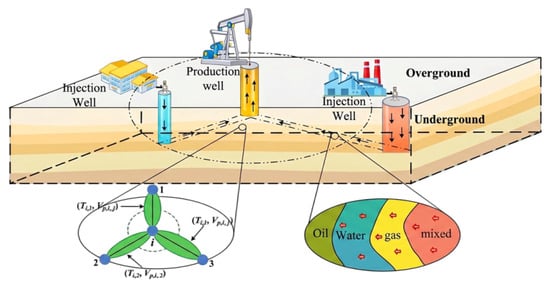
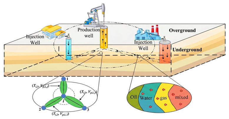
WAG flooding has been demonstrated to effectively overcome the limitations of a single displacement method by leveraging the synergistic effect of water flooding and gas flooding [6]. Injected water can block high-permeability channels and inhibit gas channeling, while injected gas can enter tiny pores to displace residual oil. The amalgamation of water and gas injection has been demonstrated to facilitate mobility control and augmented swept volume expansion [7]. Nevertheless, the complexity of reservoir dynamic connectivity and strong inter-well interference hinder precise control of the displacement path of the injected medium, frequently inducing gas or water channeling, thereby reducing displacement efficiency and increasing development costs, which severely undermines the expected performance and economic benefits of this technology. The dynamic optimization scenario of a water–gas two-flooding reservoir with inter-well connectivity is shown in Figure 1.

Figure 1. Dynamic optimization scenario diagram of WAG reservoir with inter-well connectivity.

Investigating the dynamic connectivity between wells rapidly and efficiently is of great significance for reducing development costs [8]. In the context of research into the development of artificial intelligence, existing reservoir numerical research is characterized by a paucity of a unified physical model, a deficiency that engenders considerable difficulty for researchers in non-petroleum fields, most particularly in the interdisciplinary field of artificial intelligence and petroleum. As the cornerstone of reservoir description and water flood design, inter-well connectivity has been widely applied in production performance prediction [9]. The accurate identification of inter-well connectivity is imperative for optimal injection–production well patterns, the formulation of reasonable development strategies, the prediction of residual oil distribution, and the timely suppression of ineffective circulation [10]. Inter-well connectivity directly affects the effective sweep range of the displacement medium and provides key decision support for late-stage development adjustments, thus serving as the cornerstone of refined and intelligent reservoir management.

In order to solve the core problems of low water flooding efficiency and high gas channeling risk in a complete reservoir model in high water-cut reservoirs, a reinforcement learning-based dynamic optimization strategy is proposed to solve the injection optimization problem for WAG injection with inter-well connectivity. Specifically, a net present value (NPV) model is built for a single time slot based on the oil production, the injection cost of water or gas, the conversion cost between water flooding and gas flooding, and the inter-well connectivity. Furthermore, an NPV optimization problem is formulated for multi-injection wells and multi-production wells to enhance oil recovery. Then, a Q-learning algorithm is adopted for solving the proposed optimization problem to achieve the optimal WAG injection strategy, in which the state space comprises pressure and three-phase saturation, the action space includes injection type and rate, and the reward function is the total recovery benefit. Finally, extensive numerical simulations are conducted. The experimental results imply that the proposed WAG strategy can obtain higher NPV than that of the benchmark algorithms. The main contributions are shown as follows.

(1)

A net present value model is built for multiple time slots to evaluate the relationships among oil production, the injection cost of water or gas, the conversion cost between water flooding and gas flooding, and the inter-well connectivity.

(2)

The NPV optimization problem is formulated as the Markov Decision Process, and the Q-learning algorithm is used to achieve the optimal WAG injection strategy.

(3)

The extensive simulation experiments are conducted to verify the performance of proposed algorithms on NPV.

The remainder of this paper is organized as follows. Section 2 reviews the related work on machine learning applications in reservoir optimization, WAG injection, and inter-well connectivity analysis. Section 3 describes the system model in detail, including production calculation, injection well pressure calculation, material balance equation, saturation updating, and relative permeability updating, followed by the problem formulation with NPV as the objective function. Section 4 presents the WAG injection model based on reinforcement learning, covering the definitions of state space, action space, and reward function, as well as the Q-learning algorithm design. Section 5 introduces the numerical simulation setup, benchmark strategies, and evaluation metrics, and then presents and analyzes the simulation results. Finally, Section 6summarizes the conclusions and discusses future work.

2. Related Works

Machine learning (ML) significantly reduces computational time and cost within an acceptable accuracy range [11,12]. In recent years, ML-based methods have been widely used in reservoir optimization and EOR research [13,14]. Cheraghi et al. [15] used artificial neural network (ANN) and random forest (RF) models to screen the most suitable methods for EOR.

In the optimization of water injection development, Ma et al. [16] integrated a deep neural network (DNN) into reinforcement learning to optimize the water injection rate to improve oil recovery and obtain maximum economic value, and finally achieved a low water cut and stable oil production rate. Farahi et al. [17] realized the long-term and short-term prediction of reservoir economic value by improving the multi-objective particle swarm optimization algorithm.

The above studies are based on the optimization of water injection development reservoirs to improve oil recovery, and do not consider the displacement benefits of water flooding and gas flooding. Wu et al. [18] innovatively proposed a radio frequency-based scoring method for CO₂-EOR in middle and deep reservoirs to evaluate the feasibility and reliability of CO₂-EOR in reservoirs. Dudek et al. [19] used a genetic algorithm (GA) to optimize the development strategy of multi-level oil and gas reservoirs, indicating that this method has broad application prospects. Almost all of the above studies independently optimize multiple different problems and ignore the potential synergy between them. However, they rarely exist independently in actual reservoir problems. Yao et al. [20] introduced a new multi-task optimization method, multi-factor evolutionary algorithm (MFEA), to solve the problem of production optimization, and studied the production optimization of different intensities through the correlation between problems.

At present, most of the methods or models applying ML to the study of EOR by carbon dioxide flooding focus on predicting oil recovery and NPV function calculation. However, they do not consider the cost of carbon dioxide injection and recovery [21]. The existing methods lack rapid screening and optimization of different types of injection schemes, and the inter-well connectivity and fluid flow capacity are not considered in the existing studies. Moreover, most ML models are black-box models, and their low interpretability poses challenges for result verification and method understanding.

The interpretability of ML models has been widely studied in fields such as biomedicine and material chemistry, but it is rarely used in the oil industry [22,23]. Wen et al. [24] developed a new interpretable ML framework to explain the fluid flow problems in multi-scale porous media. The developed framework can quickly screen out suitable carbon dioxide flooding strategies according to reservoir conditions. In practical applications, carbon dioxide flooding will lead to gas channeling. In order to have a higher interpretability to describe the flow of gas in the ground, Zhuang et al. [25] proposed a CO₂ flooding and storage method based on deep learning, focusing on solving the problem of gas channeling, and proposed an interpretable CO₂ flooding connectivity coefficient formula.

The above studies only consider the reservoir optimization problem under one injection condition, but in the middle and late stages of reservoir development, the problem of high water cuts is prominent. The gas channeling problem induced by single-gas injection can also adversely affect development benefits, whereas WAG injection can effectively maintain formation pressure [26]. Kanaani et al. [27] addressed the challenges of middle- and late-stage reservoir development by optimizing the CO₂-WAG injection process, which enables carbon dioxide storage in the reservoir while simultaneously enhancing oil recovery. Asante et al. [28] used time series analysis to predict the recovery of CO₂-EOR reservoirs, focusing on the inverted five-point model. The dynamic data, including pressure, WAG period and injection volume, are preprocessed and divided by time. Sensitivity analysis shows the importance of WAG period adjustment. Liu et al. [29] conducted a comparative analysis of the multi-scale oil recovery performance of glutenite reservoirs under miscible and immiscible conditions, investigating the effects of the water–gas ratio and the injection rate on recovery efficiency.

The above research considers the reservoir optimization problem of WAG injection and analyses the effect on oil recovery under miscible flooding, but does not consider the influence of inter-well connectivity on the displacement effect. Yuan et al. [30] proposed an analytical model based on inter-well interference, which improved the prediction accuracy of dynamic response but did not consider heterogeneity. Kumar et al. [31] introduced the attention mechanism into the long-term and short-term memory neural network to achieve production prediction, but did not incorporate reservoir physical parameters. Guo [32] proposed a new dynamic inter-well connectivity model and studied the core factors affecting the inter-well fluid flow by using the extended Kalman filter method. Their results show that the absolute permeability is the main factor affecting the inter-well connectivity coefficient of the one-injection and one-production system. However, the above article does not carry out the next analysis of the recovery rate.

In summary, existing studies on reservoir development optimization have made significant progress in water flooding optimization [16,17], CO₂-EOR screening [18,19], and WAG injection parameter analysis [27,28,29]. However, most of these studies suffer from three major limitations. First, they typically focus on a single injection condition (either water flooding or gas flooding alone) and fail to jointly optimize both injection mode and injection rate in a unified framework. Second, inter-well connectivity, which critically affects sweep efficiency and displacement path control in heterogeneous reservoirs, is often neglected in the optimization process. Third, the majority of existing ML-based approaches employ black-box models with limited interpretability, making it difficult to verify the physical consistency of the obtained strategies. To address these gaps, our work proposes a reinforcement learning-based WAG injection optimization framework that explicitly incorporates inter-well connectivity into the system model, jointly optimizes injection type and rate using Q-learning, and maintains physical interpretability through a transparent state–action–reward design based on reservoir mechanisms.

3. System Model

An oil-field secondary development system with $M$ injection wells and $N$ production wells is considered. The set of injection wells is represented by $\mathcal{I}=\{1,2,\dots ,M\}$. The set of production wells is denoted by $\mathcal{P}=\{1,2,\dots ,N\}$. In this system, each injection well is responsible for maintaining pressure and fluid displacement within its controlled drainage area, and direct communication or fluid exchange between injection wells is not considered under normal operating conditions. The set of production wells influenced by a specific injection well $i$ is defined as the response group ${\mathcal{P}}_i$.

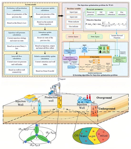
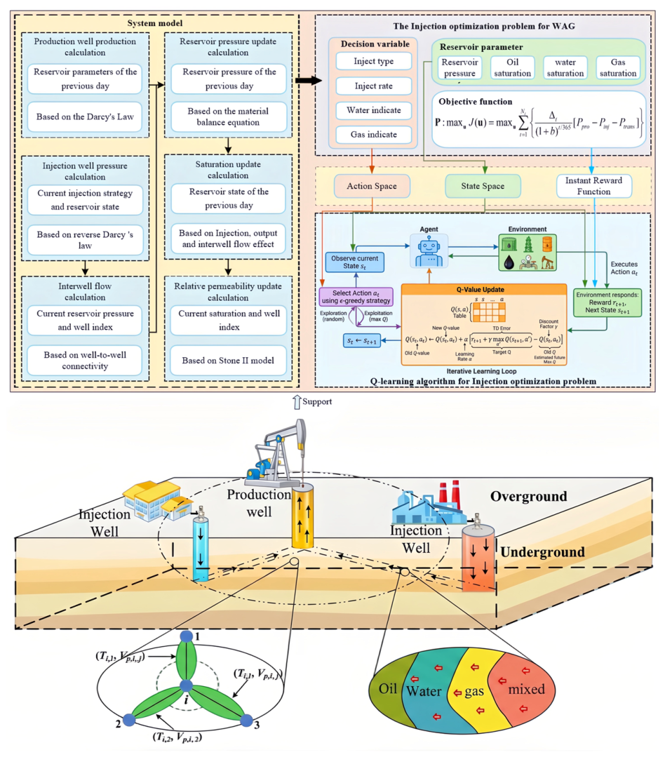
The overview of the research is shown in Figure 2. Without loss of generality, an injection well may execute a multi-phase injection assignment in a given operational cycle, and the injection stream is assumed to be separable into distinct fluid components: water, gas, and chemical agents. If the fluid medium cannot be physically separated downhole, the medium is treated as a single composite slug. Consequently, the fluid phases can propagate simultaneously through the porous medium, achieving miscible displacement. In other words, the injected medium can either displace residual oil as a sweeping agent or alter interfacial tension as a miscible solvent.

Figure 2. Overview of research in this article.

3.1. Production Calculation Model

In this paper, the method of combining the well model with Darcy’s law is used to calculate the production of production wells. The constant BHP production mode is adopted in the production well, and the optimal injection strategy is obtained by optimizing the objective function of the injection well through the agent, whose specific expression is as follows.

The underground volumetric flow rate needs to be converted into a production rate under standard surface conditions through the volumetric coefficient. Let $q_{op}(t)$, $q_{wp}(t)$ and $q_{gp}(t)$ represent the ground oil production (STB/D), ground water production (STB/D) and ground gas production (MCF/D) during time slot $t$, respectively, which are expressed, successively, as follows.

$$q_{op}(t)={\displaystyle \sum _{l=1}^{N_l}\frac{W{I}_l\cdot {\lambda }_o(t-1)\cdot (p_{res}(t-1)-p_{wf}(t-1))}{B_o}}$$

(1)

$$q_{wp}(t)={\displaystyle \sum _{l=1}^{N_l}\frac{W{I}_l\cdot {\lambda }_w(t-1)\cdot (p_{res}(t-1)-p_{wf}(t-1))}{B_w}}$$

(2)

$$q_{gp}(t)={\displaystyle \sum _{l=1}^{N_l}\frac{W{I}_l\cdot {\lambda }_g(t-1)\cdot (p_{res}(t-1)-p_{wf}(t-1))}{B_g}+q_{op}(t)\cdot R_s(t-1)}$$

(3)

where $N_l$ represents the total number of layers; ${\lambda }_o(t-1)$, ${\lambda }_w(t-1)$ and ${\lambda }_g(t-1)$ represent the flow rates of the oil, water, and gas phases at time slot $t-1$, respectively, which are defined by ${\lambda }_o(t-1)=k_{ro}(t-1)/{\mu }_o(t-1)$, ${\lambda }_w(t-1)=k_{rw}(t-1)/{\mu }_w(t-1)$ and ${\lambda }_g(t-1)=k_{rg}(t-1)/{\mu }_g(t-1)$, successively; $p_{res}(t-1)$ is the average reservoir pressure (psi) at time slot $t-1$; $p_{wf}$ represents the constant bottom-hole flowing pressure (psi) at time slot $t-1$; $B_o$, $B_w$ and $B_g$ are the volume coefficients of oil, water, and gas, respectively; $R_s(t-1)$ is the Solution Gas–Oil Ratio; and $W{I}_l$ is the well index (bbl/d) for each layer.

Based on the geometric parameters of the reservoir and the well completion conditions, the well index (WI) for each layer is calculated. For the $l-th$ layer, the expression of the $W{I}_l$ is

$$W{I}_l={\displaystyle \frac{0.00708\cdot k_l\cdot h_l}{\ln (r_e/r_w)-0.75+s}}$$

(4)

where $k_l$ represents the absolute permeability (mD) of $l-th$; $h_l$ is the effective thickness (ft) of $l-th$; $r_e$ and $r_w$ are the oil leakage (ft) and the wellbore radius (ft), respectively; $s$ is the skin factor; and the constant 0.00708 is the unit conversion factor. This formula is based on the equivalent well diameter method proposed by Peaceman (1978) [33] and is applicable to well processing in rectangular grids.

3.2. Injection Well Pressure Calculation Model

The injection well adopts a constant-rate injection mode. The type of injected fluid (water or gas) is determined by the injection strategy, and the injection rate is limited by the equipment capacity. Darcy’s law is used to deduce the injection well pressure, which the core idea is to deduce the required BHP by WI and fluid properties under the condition of known injection rate and current reservoir pressure. Let $p_{inj}(t)$ denotes the BHP of the injection well at time slot $t$, and the specific performance is the well-controlled reservoir pressure plus injection pressure, which is expressed as follows.

$$p_{inj}(t)=p_{res}(t-1)+{\displaystyle \frac{q_{inj}(t)\cdot B_{inj}\cdot \gamma }{W{I}_{total}\cdot {\lambda }_{inj}(t)}}$$

(5)

where $p_{res}(t-1)$ denotes well control reservoir pressure of injection well at time slot $t-1$; $B_{inj}$ represents the volume coefficient of injected fluid; for gas injection, $\gamma =1000$ will convert MCF to SCF, and for water injection, $\gamma =1$; $W{I}_{total}={\displaystyle \sum _{l=1}^{N_l}W{I}_l}$ represents the total well index for the entire well; ${\lambda }_{inj}(t)$ represents the flow rates of the injected fluid at time slot $t$; and $q_{inj}(t)$ denotes the actual injection rate at time slot $t$.

Considering the bearing capacity of the wellbore, after injecting the target with a rate of $q_{input}$, the actual injection rate is

$$q_{inj}=\left\{\begin{array}{c}\min (q_{input},q_{\max ,water})\\ \min (q_{input},q_{\max ,gas})\end{array}\right.$$

(6)

where $q_{\max ,water}$ and $q_{\max ,gas}$ represent the maximum allowable water injection rate and the gas injection rate respectively.

3.3. Material Balance Equation

The following considers the inflow and outflow of oil and water within the connected unit, in addition to the compressibility of oil, gas, water, and rock, and neglects inter-layer channeling and capillary forces [34]. Taking the $x-th$ well as the object, the material balance equation under reservoir conditions is as follows.

$${\displaystyle {\displaystyle \sum _{l=1}^{N_l}}{\displaystyle \sum _{y=1}^{N_w}{T}_{x,y,l}(t)}{p}_y(t)}-p_x(t){\displaystyle {\displaystyle \sum _{l=1}^{N_l}}{\displaystyle \sum _{y=1}^{N_w}{T}_{x,y,l}(t)}}+q_x(t)={\displaystyle \frac{d{p}_v(t)}{dt}}{\displaystyle {\displaystyle \sum _{l=1}^{N_l}}{C}_{t,l}{V}_{x,l}(t)}$$

(7)

The implicit difference of (7) can be obtained.

$${\displaystyle {\displaystyle \sum _{l=1}^{N_l}}{\displaystyle \sum _{y=1}^{N_w}{T}_{x,y,l}(t)p_y(t)-}}{p}_x(t){\displaystyle {\displaystyle \sum _{l=1}^{N_l}}{\displaystyle \sum _{y=1}^{N_w}{T}_{x,y,l}(t)+q_x(t)=\frac{p_x(t)-p_x(t-1)}{\Delta t}}}{\displaystyle {\displaystyle \sum _{l=1}^{N_l}}{C}_{t,l}{V}_{x,l}(t)}$$

(8)

where $p_x(t)$ and $p_y(t)$ are the average pressure (psi) of the well $x$ and the well $y$ in the drainage area at time slot $t$; $q_x(t)$ is the flow rate of the well $x$ during time slot $t$, where $q_x(t)>0$ if $x\in \mathcal{I}$, and $q_x(t)<0$ if $x\in \mathcal{P}$; $\Delta t$(day) is the time step; $C_{t,l}$ is the comprehensive compression coefficient of reservoir of the $l-th$ layer; $V_{x,l}(t)$ denotes the drainage volume ($m^3$) of well $x$ of the $l-th$ layer at time slot $t$; and $T_{x,y,l}(t)$ represents the average inter-well conductivity ($m^3/(\mathrm{d}\cdot Psi)$) of the well $x$ and the well $y$ of the $l-th$ layer at time slot $t$. According to the percolation theory, the conductivity and connected volume change with time, which can be estimated based on the pressure or saturation at the previous time.

$$T_{x,y,l}(t)=11.57{\displaystyle \frac{A_{x,y,l}{\lambda }_{x,y,l}(t-1)}{L_{x,y,l}}}=T_{x,y,l}(0){\displaystyle \frac{{\lambda }_{x,y,l}(t-1)}{{\lambda }_{x,y,l}(0)}}$$

(9)

$$V_{x,l}(t)=V_{x,l}(0)[1+C_{t,l}(p_x(t-1)-p_x(0))]$$

(10)

where $A_{x,y,l}$ represents the average seepage cross-sectional area between the well $x$ and the well $y$ at the $l-th$ layer; $L_{x,y,l}$ is the well distance between the well $x$ and the well $y$ at the $l-th$ layer; and ${\lambda }_{x,y,l}(t-1)$ represents mobility of the reservoir at time slot $t-1$, which is expressed as

$${\lambda }_{x,y,l}(t)=\left\{\begin{array}{c}\begin{array}{ll}{\lambda }_{x,l}(t-1)=& k_{x,y,l}[{\displaystyle \frac{k_{ro}(S_{o,x,l}(t-1),S_{g,x,l}(t-1))}{{\mu }_{o,l}}}+{\displaystyle \frac{k_{rw}(S_{w,x,l}(t-1))}{{\mu }_{w,l}}}+\\ & {\displaystyle \frac{k_{rg}(S_{g,x,l}(t-1))}{{\mu }_{g,l}}}],p_x(t-1)\ge p_y(t-1)\end{array}\\ \begin{array}{ll}{\lambda }_{y,l}(t-1)=& k_{x,y,l}[{\displaystyle \frac{k_{ro}(S_{o,y,l}(t-1),S_{g,y,l}(t-1))}{{\mu }_{o,l}}}+{\displaystyle \frac{k_{rw}(S_{w,y,l}(t-1))}{{\mu }_{w,l}}}+\\ & {\displaystyle \frac{k_{rg}(S_{g,y,l}(t-1))}{{\mu }_{g,l}}}],p_x(t-1)<p_y(t-1)\end{array}\end{array}\right.$$

(11)

where $k_{x,y,l}$ denotes the average permeability of the well $x$ and the well $y$ in layer $l$; $k_{ro}$, $k_{rw}$, $k_{rg}$ represent the relative permeability of oil phase, water phase and gas phase, respectively; $S_{o,x,l}(t-1)$, $S_{w,x,l}(t-1)$ and $S_{g,x,l}(t-1)$ are the oil phase saturation, water phase saturation and gas phase saturation of well $x$ at time slot $t-1$, respectively; and ${\mu }_{o,l}$, ${\mu }_{w,l}$ and ${\mu }_{g,l}$ are oil, water and gas viscosity, respectively.

The formula describes the comprehensive migration ability of the fluid in porous media when it starts from the upstream well, overcomes its own viscous resistance and is controlled by rock permeability, and carries oil, water and gas three-phase flow to the downstream well.

3.4. Saturation Update Calculation Formulation

In this paper, the saturation update is determined by the time slot $t-1$ saturation and the saturation variations induced by injected energy at time slot $t$, including produced fluid, and inter-well flow. Let $S_{o,inj,l}(t)$ and $S_{o,pro,l}(t)$, $S_{w,inj,l}(t)$ and $S_{w,pro,l}(t)$, and $S_{g,inj,l}(t)$ and $S_{g,pro,l}(t)$ denote oil phase, water phase, and gas phase saturation in injection well or production well at time slot $t$ in the $l-th$ layer, which are expressed as follows.

$$S_{o,inj,l}(t)=S_{o,inj,l}(t-1)+\Delta S_{o,inj,l}(t)+\Delta S_{o,inj,flow}(t)$$

(12)

$$S_{w,inj,l}(t)=S_{w,inj,l}(t-1)+\Delta S_{w,inj,l}(t)+\Delta S_{w,inj,flow}(t)$$

(13)

$$S_{g,inj,l}(t)=S_{g,inj,l}(t-1)+\Delta S_{g,inj,l}(t)+\Delta S_{g,inj,flow}(t)$$

(14)

$$S_{o,pro,l}(t)=S_{o,pro,l}(t-1)+\Delta S_{o,pro,l}(t)+\Delta S_{o,pro,flow}(t)$$

(15)

$$S_{w,pro,l}(t)=S_{w,pro,l}(t-1)+\Delta S_{w,pro,l}(t)+\Delta S_{w,pro,flow}(t)$$

(16)

$$S_{g,pro,l}(t)=S_{g,pro,l}(t-1)+\Delta S_{g,pro,l}(t)+\Delta S_{g,pro,flow}(t)$$

(17)

where $\Delta S_{o,inj,l}(t)$, $\Delta S_{w,inj,l}(t)$ and $\Delta S_{g,inj,l}(t)$ represent the three-phase change caused by injection effect at time slot $t$, respectively; $\Delta S_{w,pro,l}(t)$, $\Delta S_{o,pro,l}(t)$ and $\Delta S_{g,pro,l}(t)$ denote the three-phase change caused by production effect at time slot $t$, respectively; and $\Delta S_{o,inj,flow}(t)$, $\Delta S_{w,inj,flow}(t)$ and $\Delta S_{g,inj,flow}(t)$ are the three-phase change caused by the inter-well flow effect at time slot $t$.

3.4.1. Injection Effect

The injection well is only affected by the injection effect. For different injection energy types, the three-phase saturation variation formulas are as follows.

When the injection type is water, this will cause an increase in water volume in the well-controlled reservoir of the injection well in each layer, thus squeezing the oil and gas phases, resulting in the increase in the water phase and the decrease in the oil phase and the gas phase. Let $\Delta S_{w,inj,l}(t)$, $\Delta S_{o,inj,l}(t)$ and $\Delta S_{g,inj,l}(t)$ denote the water, oil and gas phases of the production well at time slot $t$ in the $l-th$ layer, which are expressed as follows.

$$\Delta S_{w,inj,l}(t)=+{\displaystyle \frac{V_{layer}}{V_{pore}}}=+{\displaystyle \frac{q_{wi}(t)\cdot B_w\cdot \Delta t/N_l}{\pi r_e^2\cdot h_l\cdot \varphi }}$$

(18)

$$\Delta S_{o,inj,l}(t)=-{\displaystyle \frac{V_{layer}}{V_{pore}}}=-{\displaystyle \frac{q_{wi}(t)\cdot B_w\cdot \Delta t/N_l}{\pi r_e^2\cdot h_l\cdot \varphi }}$$

(19)

$$\Delta S_{g,inj,l}(t)=-{\displaystyle \frac{V_{layer}}{V_{pore}}}=-{\displaystyle \frac{q_{wi}(t)\cdot B_w\cdot \Delta t/N_l}{\pi r_e^2\cdot h_l\cdot \varphi }}$$

(20)

Similarly, when the injection type is gas, this will cause an increase in gas volume in the well-controlled reservoir of the injection well in each layer, thus squeezing the oil and water phases, resulting in the increase in the gas phase and the decrease in the oil phase and the water phase. Let $\Delta S_{g,inj,l}(t)$, $\Delta S_{o,inj,l}(t)$ and $\Delta S_{w,inj,l}(t)$ denote the water, oil and gas phases of the injection well at time slot $t$ in the $l-th$ layer, which are expressed as follows.

$$\Delta S_{g,inj,l}(t)=+{\displaystyle \frac{V_{layer}}{V_{pore}}}=+{\displaystyle \frac{q_{gi}(t)\cdot B_g\cdot \Delta t/N_l}{\pi r_e^2\cdot h_l\cdot \varphi }}$$

(21)

$$\Delta S_{o,inj,l}(t)=-{\displaystyle \frac{V_{layer}}{V_{pore}}}=-{\displaystyle \frac{q_{gi}(t)\cdot B_g\cdot \Delta t/N_l}{\pi r_e^2\cdot h_l\cdot \varphi }}$$

(22)

$$\Delta S_{w,inj,l}(t)=-{\displaystyle \frac{V_{layer}}{V_{pore}}}=-{\displaystyle \frac{q_{gi}(t)\cdot B_g\cdot \Delta t/N_l}{\pi r_e^2\cdot h_l\cdot \varphi }}$$

(23)

where $V_{layer}$ denotes the distribution injection volume of each layer, which is defined by $V_{layer}=q_{wi}(t)\cdot B_w\cdot \Delta t/N_l$; $V_{pore}$ is the pore volume, which is defined by $V_{pore}=\pi r_e^2\cdot h_l\cdot \varphi$; $\varphi$ is the porosity; and $q_{wi}(t)$ and $q_{gi}(t)$ are expressed as the water injection volume and gas injection volume in the injection strategy at time slot $t$, respectively.

3.4.2. Production Effect

Analogously, in the production effect, the fluid moves out from the reservoir to the wellbore. In the unit time slot step $\Delta t$, the surface production $q_w(t)$, $q_o(t)$ and $q_g(t)$ of each phase are converted into underground output volume by the volume coefficient. Under the condition that the pore volume $V_{pore}$ of the reservoir remains unchanged, the fluid is produced, which means that the mass of the three-phase fluid in the well control area is reduced. Therefore, the water, oil and gas saturation of the production well decreases accordingly. Let $\Delta S_{w,pro,l}(t)$, $\Delta S_{o,pro,l}(t)$ and $\Delta S_{g,pro,l}(t)$ denote the variation in the production well in the $l-th$ layer at time slot $t$, which can be expressed as follows.

$$\Delta S_{w,pro,l}(t)=-{\displaystyle \frac{V_{w,layer}}{V_{pore}}}=-{\displaystyle \frac{q_w(t)\cdot B_w\cdot \Delta t/N_l}{\pi r_e^2\cdot h_l\cdot \varphi }}$$

(24)

$$\Delta S_{o,pro,l}(t)=-{\displaystyle \frac{V_{o,layer}}{V_{pore}}}=-{\displaystyle \frac{q_o(t)\cdot B_o\cdot \Delta t/N_l}{\pi r_e^2\cdot h_l\cdot \varphi }}$$

(25)

$$\Delta S_{g,pro,l}(t)=-{\displaystyle \frac{V_{g,layer}}{V_{pore}}}=-{\displaystyle \frac{q_g(t)\cdot B_g\cdot \Delta t/N_l}{\pi r_e^2\cdot h_l\cdot \varphi }}$$

(26)

where $V_{w,layer}$, $V_{o,layer}$ and $V_{g,layer}$ denote the water, oil and gas production volume affecting all production layers.

3.4.3. Inter-Well Flow Effect

In inter-well flow, the transport of fluids between injection and production wells is not single-phase but involves mixed migration of oil, water, and gas. To accurately model this process in a discrete numerical framework while rigorously preserving mass conservation, the upstream weighting scheme is employed to handle three-phase inter-well flow. The upstream well (injection well) loses fluid volume due to migration, with corresponding reductions in its water, oil, and gas saturations. The downstream well (production well) gains exactly the same volume, resulting in proportionate increases in its three-phase saturations. This approach physically reflects the principle that the displacing fluid composition is determined by the source fluid properties and numerically guarantees mass conservation between the injection wells and the production wells, thereby avoiding non-conservation issues caused by artificially assigned flow fractions. Let $\Delta S_{w,inj,flow}(t)$, $\Delta S_{o,inj,flow}(t)$ and $\Delta S_{g,inj,flow}(t)$ with $\Delta S_{w,pro,flow}(t)$, $\Delta S_{o,pro,flow}(t)$ and $\Delta S_{g,pro,flow}(t)$ denote the variation in injection well and production well in the $l-th$ layer at time slot $t$.

$$\Delta S_{w,inj,flow}(t)=-{\displaystyle \frac{\Delta V_w}{V_{pore}}}=-{\displaystyle \frac{T_{ij}(t)\cdot (P_{inj}(t)-P_{prod}(t))\cdot f_w(t)\cdot \Delta t}{\pi r_e^2\cdot h_l\cdot \varphi }}$$

(27)

$$\Delta S_{o,inj,flow}(t)=-{\displaystyle \frac{\Delta V_o}{V_{pore}}}=-{\displaystyle \frac{T_{ij}(t)\cdot (P_{inj}(t)-P_{prod}(t))\cdot f_o(t)\cdot \Delta t}{\pi r_e^2\cdot h_l\cdot \varphi }}$$

(28)

$$\Delta S_{g,inj,flow}(t)=-{\displaystyle \frac{\Delta V_g}{V_{pore}}}=-{\displaystyle \frac{T_{ij}(t)\cdot (P_{inj}(t)-P_{prod}(t))\cdot f_g(t)\cdot \Delta t}{\pi r_e^2\cdot h_l\cdot \varphi }}$$

(29)

$$\Delta S_{w,pro,flow}(t)=+{\displaystyle \frac{\Delta V_w}{V_{pore}}}=+{\displaystyle \frac{T_{ij}(t)\cdot (P_{inj}(t)-P_{prod}(t))\cdot f_w(t)\cdot \Delta t}{\pi r_e^2\cdot h_l\cdot \varphi }}$$

(30)

$$\Delta S_{o,pro,flow}(t)=+{\displaystyle \frac{\Delta V_o}{V_{pore}}}=+{\displaystyle \frac{T_{ij}(t)\cdot (P_{inj}(t)-P_{prod}(t))\cdot f_o(t)\cdot \Delta t}{\pi r_e^2\cdot h_l\cdot \varphi }}$$

(31)

$$\Delta S_{g,pro,flow}(t)=+{\displaystyle \frac{\Delta V_g}{V_{pore}}}=+{\displaystyle \frac{T_{ij}(t)\cdot (P_{inj}(t)-P_{prod}(t))\cdot f_g(t)\cdot \Delta t}{\pi r_e^2\cdot h_l\cdot \varphi }}$$

(32)

where $\Delta V_w$, $\Delta V_o$ and $\Delta V_g$ are expressed as water, oil and gas volume changes caused by various flow rates, respectively; $f_w(t)$, $f_o(t)$ and $f_g(t)$ are the flow fraction of each phase in the total mobility, respectively, which are defined by ${\lambda }_w/{\lambda }_w+{\lambda }_o+{\lambda }_g$, ${\lambda }_o/{\lambda }_w+{\lambda }_o+{\lambda }_g$ and ${\lambda }_g/{\lambda }_w+{\lambda }_o+{\lambda }_g$, successively.

3.5. Relative Permeability Update Model

In this paper, the three-phase relative permeability model is used to realize the dynamic update of relative permeability by combining the two-phase Corey empirical formula with the Stone II three-interpolating model. The specific steps are as follows.

The relative permeability of the oil phase under the condition of three-phase coexistence was calculated using the Stone II model. This model obtained the three-phase oil phase permeability by interpolating the two-phase relative permeability data. Let $k_{ro,l}(t)$ represent the relative permeability of the oil phase in the $l-th$ layer at time slot $t$, whose expression is

$$k_{ro,l}(t)=k_{rcow}\left[\left({\displaystyle \frac{k_{row,l}(t)}{k_{rcow}}}+k_{rw,l}(t)\right)\left({\displaystyle \frac{k_{rog,l}(t)}{k_{rcow}}}+k_{rg,l}(t)\right)-\left(k_{rw,l}(t-1)+k_{rg,l}(t-1)\right)\right]$$

(33)

where $k_{rcow}$ denotes the relative permeability of the bound underwater oil phase; $k_{row,l}(t)$ and $k_{rog,l}(t)$ are the oil relative permeabilities in the oil–water system and the oil–gas system at time slot $t$ in $l-th$ layer; and $k_{rw,l}(t)$ and $k_{rg,l}(t)$ represent water relative permeability and gas relative permeability at time slot $t$ in the $l-th$ layer. The formula for calculating the $k_{row,l}(t)$ and $k_{rog,l}(t)$ are

$$k_{row,l}(t)=k_{krow}^0\cdot {(1-S_{we,l}(t))}^{n_{ow}}$$

(34)

$$k_{rog,l}(t)=k_{krog}^0\cdot {(1-S_{ge,l}(t))}^{n_{og}}$$

(35)

where $k_{krow}^0$ and $k_{krog}^0$ represent the maximum relative permeability of the oil phase in the water–oil system and the relative permeability of the oil phase in the gas–oil system; $n_w$, $n_g$, $n_{ow}$ and $n_{og}$ are Corey indices; and $S_{we,l}(t)$ and $S_{ge,l}(t)$ are the effective saturation of water phase and effective saturation of gas phase in the $l-th$ layer.

Based on the Corey empirical model, the relative permeability of the two phases in the oil–water system and the oil–gas system was calculated respectively. Let $k_{rw,l}(t)$ and $k_{rg,l}(t)$ represent the relative permeability of the water phase and gas phase in the $l-th$ layer at time slot $t$, which are expressed as follows.

$$k_{rw,l}(t)=k_{rw}^0\cdot S_{we,l}^{n_w}(t)$$

(36)

$$k_{rg,l}(t)=\left\{\begin{array}{c}{k}_{rg}^0\cdot S_{ge}^{n_g}(t),S_g>S_{ge}\\ 0,S_g\le S_{ge}\end{array}\right.$$

(37)

where $k_{rw}^0$ and $k_{rg}^0$ are the maximum relative permeability of water and gas. Effective saturation of water phase $S_{we,l}(t)$ and effective saturation of gas phase $S_{ge,l}(t)$ are defined as follows.

$$S_{we,l}(t)={\displaystyle \frac{S_{w,l}(t)-S_{wc}}{1-S_{wc}-S_{orw}}}$$

(38)

$$S_{ge,l}(t)={\displaystyle \frac{S_{g,l}(t)-S_{gc}}{1-S_{wc}-S_{org}-S_{gc}}}$$

(39)

where $S_{w,l}(t)$ and $S_{g,l}(t)$ represent the saturation of the water phase and the gas phase respectively at time slot $t$ in the $l-th$ layer, $S_{wc}$ is the irreducible water saturation, and $S_{orw}$ is the residual oil saturation to water flood; $S_{org}$ is the residual oil saturation to gas flood and $S_{gc}$ is the critical gas saturation. To ensure physical rationality, the effective saturation is restricted within the range of [0, 1].

3.6. Problem Formulation

This section studies the joint optimization problem of achieving material balance, production calculation and injection strategy in the mid-to-late stage of reservoir development, addressing the issues of high water cut and economic benefits. In this paper, NPV is used to evaluate the oil displacement effect of reservoirs under known geological conditions, and the objective of this optimization problem is to maximize economic benefits. The NPV function is defined as

$$P:\underset{u}{\max }\mathrm{J}(u)=\underset{u=\{type,rate,\alpha ,\beta \}}{\max }{\displaystyle \sum _{t=1}^{N_t}\left\{\frac{{\Delta }_t}{{(1+b)}^{\frac{t}{365}}}[P_{pro}-P_{inj}-P_{trans}]\right\}}$$

(40)

s.t.

$$u^{low}\le u\le u^{up}$$

(41)

$$x^0=x_0(\mathrm{initial} \mathrm{condition})$$

(42)

$${\alpha }^t+{\beta }^t=1/0,({\alpha }^t,{\beta }^t\in \{0,1\})$$

(43)

where $u$ denotes an n-dimensional vector, including the well injection control variable; $N_t$ (days) is the total time step; ${\Delta }_t$(day) is the time at the end of the $l-th$ time step; $b$ is the annual discount factor; and $P_{pro}$, $P_{inj}$ and $P_{\mathrm{trans}}$ represent the total revenue of the production well, the injection cost of the injection well and the conversion cost associated with alternating water flooding and gas flooding across distinct time slices, respectively. Among them, the well control unit variables include water injection volume $q_{wi}$ and gas injection volume $q_{gi}$ in each time period, whose constraint range is $q_{wi}\in (0,4000)$ and $q_{gi}\in (0,20000)$. The state variable $x$ is the reservoir dynamic variable, including pressure, saturation, etc., which is the well injection control variable to ensure that the single well can only inject water or gas at each moment. $\alpha ,\beta \in \{0,1\}$ indicates whether the injection well is injected with water or gas.

The specific expressions are as follows.

$$P_{pro}=r_o{q}_{op}(t)-c_w{q}_{op}(t)-c_g{q}_{gp}(t)$$

(44)

$$P_{inj}=c_{wi}{q}_{wi}(t)\alpha (t)+c_{gi}{q}_{gi}(t)\beta (t)$$

(45)

$$P_{\mathrm{trans}}=c_{trans}\alpha (t-1)\beta (t)+c_{trans}\alpha (t)\beta (t-1)$$

(46)

where $t$ represents the time step index of simulation; $r_o$, $c_w$ and $c_g$ denote the price of crude oil, the cost factor of water treatment and the cost factor of gas treatment respectively; $q_{op}(t)$, $q_{op}(t)$ and $q_{gp}(t)$ are the oil, water and gas production for each time period of a single well at time slot $t$, respectively; $c_{wi}$ and $c_{gi}$ are the water and gas injection cost factor; $q_{wi}(t)$ and $q_{gi}(t)$ are the amount of water and gas injection for each time period at time slot $t$; and $c_{trans}$ represents the cost of converting from gas injection to water injection or water injection to gas injection. When $\alpha =1$ or $\beta =1$, this indicates that water or gas is injected. Similarly, when $\alpha =0$ or $\beta =0$, this indicates no injection. Then we know that when the value of $\alpha$ or $\beta$ changes at the current time, there will be a conversion cost, which is the agent that changes the type of injected energy.

The reservoir dynamic optimization problem can be described as follows: under the condition that the control variables (production well injection rate and bottom-hole flow pressure) satisfy the linear condition constraint $u^{low}\le u\le u^{up}$, the optimal control well control unit variables $u$ and well injection control variables $\alpha ,\beta$ that maximize the net present value of production NPV are solved.

4. WAG Inject Model of RL

In the WAG flooding optimization problem, the state space consists of pressure and three-phase saturation, while the action space comprises injection type and rate—both of which are low-dimensional and can be effectively discretized without significant loss of physical fidelity. The reward function is formulated as the daily discounted net cash flow, defined as oil revenue minus water/gas injection costs and switching costs, which is then normalized to the (−1, 1) interval using a nonlinear scaling function to stabilize Q-value updates. Under these conditions, Tabular Q-learning is adopted because it guarantees convergence to the optimal policy in such low-dimensional discrete MDPs without requiring function approximation, thus avoiding the approximation errors and training instability commonly encountered in deep reinforcement learning methods. In contrast, algorithms such as DDPG and SAC are designed for continuous control problems with high-dimensional state and action spaces; employing them in our setting would introduce unnecessary complexity and may suffer from over-parameterization, hyperparameter sensitivity, and slower convergence, without providing clear advantages over the simpler and more interpretable Tabular Q-learning approach. Since the WAG flooding development strategy involves a series of schemes over multiple time steps, production optimization can be expressed as a Markov Decision Process (MDP), which is a fundamental framework widely used to solve sequential decision-making problems. This MDP is defined by an artificial intelligence agent that interacts with the environment, including: state space S, action space A, state transition P, and reward function R.

4.1. Define State Space

The design of the state space must satisfy the Markov property, which requires that the next state depends solely on the current state. In the WAG injection problem, reservoir performance is mainly determined by pressure distribution and three-phase saturation. In this study, four key variables at the production well are selected to form the state vector.

$$s_t=[p,S_o,S_w,S_g]$$

(47)

where $p$ denotes the reservoir pressure at the production well, $\mathrm{psi}$; $S_o$, $S_w$ and $S_g$ are the average oil saturation, average water saturation and average gas saturation of each layer of the production well, respectively, and are dimensionless.

In order to improve the convergence stability of the Q-learning algorithm, the continuous state variables are normalized:

$$\tilde{p}={\displaystyle \frac{p}{p_{\max }}},p_{\max }=5000 psi$$

(48)

The saturation variable itself is in the $[0,1]$ interval, and no additional normalization is required. The final state vector is

$$s_{norm}={[\tilde{p},S_o,S_w,S_g]}^T\in {ℝ}^4$$

(49)

Since Q-learning stores Q-values in a tabular form, continuous states must be discretized into a finite number of lattices. The normalized pressure range [0, 1] is divided into six bins, while the normalization ranges for oil, water, and gas saturations—[0.1, 0.8], [0.15, 0.85], and [0, 0.35]—are divided into five, five, and four bins, respectively.

4.2. Define Action Space

In this system, the action space encompasses a binary group, which consists of inject type and inject rate. Where $type\in \left\{-1,0,1\right\}$, −1 means no injection, 0 means water injection, and 1 means gas injection; $rate$ denotes injection rate (STB/D for water, MCF/D for gas). The action space for the agent is designated according to (40).

$$a_t=(type,rate)$$

(50)

In action selection strategy. The agent uses the $\epsilon -greedy$ strategy for action selection, which gradually decays from 1.0 to a minimum of 0.01 to balance exploration and utilization. The expression is as follows.

$$\pi (a|s)=\left\{\begin{array}{c}1-\epsilon +{\displaystyle \frac{\epsilon }{\left|A\right|}}, \mathrm{if} a=\arg {\max }_{a^{\prime }}Q(s,a^{\prime })\\ {\displaystyle \frac{\epsilon }{\left|A\right|}},otherwise\end{array}\right.$$

(51)

4.3. Reward Function

The reward function is the most critical design element in reinforcement learning, which directly determines the optimization goal of the agent. In this system, the ultimate aim is to optimize the injection strategy to maximize the cumulative sum of NPVs, calculated at each discrete time step. This serves as a key indicator of the agent’s efficacy in enhancing oil recovery through the use of injection. Reward function is designed as follows.

$$R_t={\displaystyle \sum _{t=1}^{N_t}\left\{\frac{{\Delta }_{t_n}}{{(1+b)}^{\frac{t_n}{365}}}[P_{pro}-P_{inj}-P_{trans}]\right\}}$$

(52)

The reward function represents the total output value of the well in a one-year cycle minus the total injection cost and conversion cost, for which parameters have been introduced in the system model. Considering the time value of funds, cash flow are discounted on a daily basis.

$$C{F}_t^{\mathrm{disc}}=\left(P_{pro}-P_{inj}-P_{trans}\right)\times {\displaystyle \frac{1}{{({(1+b)}^{1/365})}^t}}$$

(53)

In order to stabilize the training process, the discounted cash flow is nonlinearly scaled:

$$r_{\mathrm{economic}}=\tanh \left(\frac{C{F}_t^{\mathrm{disc}}}{50,000}\right)$$

(54)

This function maps rewards to the (−1, 1) interval, avoiding the interference of extreme values in Q-value updates.

According to the following analysis, the pseudocode of the proposed Q-Learning algorithm is shown in Algorithm 1. At the beginning, the Q-table $Q(s,a)$ is initialized with small random values, and the simulation environment is established with the predefined action space and random seed (Algorithm 1, lines 1–4). For each training episode, the initial system state is observed from the environment and discretized into a finite lattice representation (Algorithm 1, lines 5–6). The agent then enters the daily decision loop, where an action $a_t$ is selected using the $\epsilon -$ greedy policy based on the current discretized state $s_t$ (Algorithm 1, lines 7–14). Once the action $a_t$ is executed, the environment updates the reservoir state and the next state $s_{t+1}$ is observed and discretized (Algorithm 1, lines 15–16). The reward $r_t$, which is the NPV contribution of that day, is then normalized to stabilize training (Algorithm 1, line 17). Based on the received reward and the next state, the temporal-difference (TD) target is computed, and the Q-table is updated by minimizing the clipped TD error (Algorithm 1, lines 18–28). After each episode, the cumulative NPV is calculated, and the optimal policy is updated if the current episode achieves a higher NPV than the historical best (Algorithm 1, lines 29–34). Finally, the learning rate and exploration rate are decayed to gradually shift from exploration to exploitation (Algorithm 1, lines 35–36).

The time complexity of the proposed Q-learning algorithm depends on the Q-table lookup and update operations. Let $\mathcal{S}$ and $\mathcal{A}$ denote the sizes of the discretized state space and action space, respectively, with $\mathcal{S}$ = 600 and $\mathcal{A}$ = 16. Let $E$ be the number of training episodes and $T$ be the number of time steps per episode. At each step, the algorithm performs a Q-table lookup of complexity $O(\mathcal{A})$ and a Q-value update of complexity $O(1)$. Thus, the overall time complexity is estimated as $O(E\cdot T\cdot \mathcal{A})$, which scales linearly with the number of episodes, time steps, and action space size.

Algorithm 1: Q-learning Algorithm for WAG Injection Optimization

Input: Initialize the Q-table $Q(s,a)$ with small random values, state discretization bins $\mathcal{B}$, learning rate $\alpha$, discount factor $\gamma$, initial exploration rate $\epsilon$, exploration rate decay parameters, and the simulation horizon $T=365$ days.

Output: Optimal Q-table $Q^{\ast }$, optimal policy ${\pi }^{*}$, and best cumulative NPV.

1: Initialize the WAG environment ${\rm E}$ with action space $S$ and random seed

2: For each episode $\mathrm{ep}=1$ to $N_{\mathrm{episodes}}$ do

3:  $s_0\leftarrow E.\mathrm{reset}()$ //Observe initial state

4:  $s_t^{\mathrm{idx}}\leftarrow \mathrm{discretize}(s_t,\mathcal{B})$//Discretize continuous state

5:  For each day $t=0$ to $T-1$ do//Make decisions and updates by day

6:   Select action using $\epsilon \text{-}$greedy policy://Choose action

7:   If $\mathrm{random}()<\epsilon$ then

8:    $a_t\leftarrow \mathrm{Uniform}(A)$//Exploration random

9:   Else

10:    $a_t\leftarrow \arg {\max }_{a}Q(s_t^{\mathrm{idx}},a)$//Exploitation from Q-table

11:   End If

12:    $s_{t+1},r_t,\mathrm{done}\leftarrow E.\mathrm{step}(a_t)$//Execute action $a_t$

13:    $s_{t+1}^{\mathrm{idx}}\leftarrow \mathrm{discretize}(s_{t+1},\mathcal{B})$//Discretize next state

14:    ${\tilde{r}}_t\leftarrow \mathrm{normalize}(r_t)$//Normalize reward

15:   Compute TD target:

16:   If done then

17:    $y_t={\tilde{r}}_t$//Update the target value

18:   Else

19:    $y_t={\tilde{r}}_t+\gamma {\max }_{a^{\prime }}Q(s_{t+1}^{\mathrm{idx}},a^{\prime })$//Update the target value

20:   End If

21:   Compute TD error and update Q-table:

22:   ${\delta }_t=y_t-Q(s_t^{\mathrm{idx}},a_t)$//Calculate TD error

23:   ${\delta }_t^{\mathrm{clipped}}=\mathrm{clip}({\delta }_t,-{\delta }_{\max },{\delta }_{\max })$//Clipping TD error

24:   $Q(s_t^{\mathrm{idx}},a_t)\leftarrow Q(s_t^{\mathrm{idx}},a_t)+\alpha \cdot {\delta }_t^{\mathrm{clipped}}$//Q-value update

25:   $Q(s_t^{\mathrm{idx}},a_t)\leftarrow \mathrm{clip}(Q(s_t^{\mathrm{idx}},a_t),-Q_{\max },Q_{\max })$//Clipping Q-value

26:   $s_t\leftarrow s_{t+1}$//Assign the next state to the current state

27:   If done then break

28:  End For

29:  Compute episode NPV: ${\mathrm{NPV}}_{\mathrm{total}}\leftarrow E.\mathrm{get}\_\mathrm{total}\_\mathrm{npv}()$

30:  Update best policy if improved:

31:  If ${\mathrm{NPV}}_{\mathrm{total}}>{\mathrm{NPV}}_{\mathrm{best}}$ then

32:   ${\mathrm{NPV}}_{\mathrm{best}}\leftarrow {\mathrm{NPV}}_{\mathrm{total}}$

33:   ${\pi }^{*}\leftarrow \mathrm{recorded} \mathrm{actions}$

34:  End If

35:  Decay learning rate: $\alpha \leftarrow \max (\alpha \cdot {\alpha }_{\mathrm{decay}},{\alpha }_{\min })$

36:  Update exploration rate: $\epsilon \leftarrow decay(\epsilon )$

37: End For

38: Return $Q,{\pi }^{*},{\mathrm{NPV}}_{\mathrm{best}}$

5. Numerical Simulation and Analysis

This study is conducted on a high water-cut reservoir model with three injection wells and five production wells. Four algorithms are compared: QDOA-IR-WF (water flooding with rate optimization), QDOA-IR-GF (gas flooding with rate optimization), QDOA-IMGIR-WAGF (WAG flooding with mode optimization only, fixed rates of 2000 STB/D for water and 11,000 MCF/D for gas), and the proposed QDOA-IMR-WAGF (WAG flooding with joint optimization of both mode and rate). All algorithms share identical reservoir conditions and operating limits, with a simulation horizon of 365 days. A fixed random seed is adopted in all experiments to ensure reproducibility.

5.1. Experiment Environment

The performance of the proposed Q-learning algorithm is verified on one personal computer, whose configuration information consists of an Intel Core i5-14500 CPU@2.10 GHz, with RAM 32.0 GB, DISK 1024 GB, and the Windows 10 operating system. The Python language is adopted using version Python 3.10, and the Python-integrated development environment is PyCharm Community Edition 2023.1. The reservoir model is constructed using the CMG package to generate a 20 × 20 × 3 grid map with each grid size of 25 × 25, consisting of three injection wells and five production wells. For the performance verification of the Q-learning algorithm, the parameter settings for simulation are given in Table 1, the experiment parameters adopted in this article, where the reservoir parameters $u$, reservoir time-off state $x_0$ and system model update parameters, respectively, are shown.

Table 1. The experiment parameters adopted in this article.

Parameters	Value	Parameters	Value	Parameters	Value
$S_w$	0.6	$k_{rg}^0$	0.50	$n_{ow}$	2.2
$S_o$	0.35	$k_{krow}^0$	0.80	$n_{og}$	1.5
$S_g$	0.05	$k_{krog}^0$	0.70	$r_o$	80.0 $/STB
$S_{wc}$	0.20	$k_{rocw}$	0.90	$c_w$	4.93 $/STB
$S_{orw}$	0.25	$p$	3000 psi	$c_g$	1.42 $/MCF
$S_{org}$	0.15	$b$	0.1	$c_{wi}$	3.0 $/STB
$S_{gc}$	0.05	$n_w$	2.5	$c_{gi}$	1.42 $/MCF
$k_{rw}^0$	0.30	$n_g$	1.8	$c_{trans}$	3000 $/Times

5.2. Benchmark Algorithm

In order to verify the performance of proposed algorithm, i.e., Q-learning-based dynamic Optimization algorithm of injection mode and rate for WAG flooding (QDOA_IMR_WAGF), the Q-learning-based dynamic Optimization algorithm of injection rate for water flooding (QDOA_IR_WF), the Q-learning-based dynamic Optimization algorithm of injection rate for gas flooding (QDOA_IR_GF) and the Q-learning-based dynamic Optimization algorithm of injection mode with given injection rate for WAG flooding (QDOA_IMGIR_WAGF) are taken as the benchmark algorithms. The detailed descriptions of each benchmark algorithm are shown as follows.

QDOA-IR-WF: The algorithm uses water for displacement, and the agent can select the injection rate to provide the development strategy.

QDOA-IR-GF: The algorithm uses gas for displacement, and the agent can select the injection rate to provide the development strategy.

QDOA-IMGIR-WAGF: The algorithm uses a water–gas two-phase option for displacement, and has two injection mode selections and two fixed injection rate actions to provide injection strategies.

In order to compare the effects of different WAG strategies, four action space configurations are designed, as shown in Table 2 Comparison of four injection strategy parameters.

Table 2. Comparison of four injection strategy parameters.

Configuration	Action Type	Rate Options	Total Actions
QDOA_IMR_WAGF	Water/Gas/No	Water: [500, 1000, 1500, 2000, 2500, 3000, 3500, 4000] Gas: [2000, 5000, 8000, 11,000, 14,000, 17,000, 20,000]	16
QDOA-IR-WF	Water/No	Water: [500, 1000, 1500, 2000, 2500, 3000, 3500, 4000]	8
QDOA-IR-GF	Gas/No	Gas: [2000, 5000, 8000, 11,000, 14,000, 17,000, 20,000]	7
QDOA-IMGIR-WAGF	Water/Gas/No	Fixed: water 2000, gas 11,000	3

5.3. Metrics

In the experiment, NPV is used as an economic value evaluation index, and numerical simulation is carried out according to each convergent injection strategy to present the development effect. The development effect indexes, such as reservoir water content, saturation and remaining oil distribution, will also be presented as evaluation indexes.

NPV: NPV is the discounted sum of all cash inflows and outflows over the entire development horizon, representing the cumulative economic benefit of a reservoir development project. A higher NPV indicates better economic performance, which reflects greater profitability and more efficient resource utilization.

Three-Phase Production Rates: The three-phase production rates refer to the volumes of oil, water, and gas produced per unit time from a production well, directly reflecting reservoir development performance and displacement efficiency. A higher oil production rate is desirable, indicating effective oil recovery. A lower water production rate is preferred, as high water cut implies water channeling. Gas production rate should be maintained within a reasonable range to avoid gas channeling or insufficient gas flooding benefit.

Pressure: Pressure refers to the bottom-hole pressure or well-controlled reservoir pressure at injection and production wells, reflecting the stability of reservoir energy and fluid flow. Smooth pressure variation is desirable, indicating stable displacement and effective energy management, while severe pressure fluctuation is undesirable, which represents unstable injection or production and potential formation damage.

Three-phase Saturation: Three-phase saturation refers to the volume fractions of oil, water, and gas occupying the pore space in a reservoir, directly characterizing the distribution and displacement status of each phase. Lower water saturation and higher oil saturation are desirable, indicating effective oil displacement and delayed water breakthrough; gas saturation should be maintained within a reasonable range, as excessively high gas saturation may lead to gas channeling and reduced sweep efficiency.

Three-Phase Relative Permeability: Three-phase relative permeability refers to the effective permeability of oil, water, or gas phase relative to the absolute permeability of the reservoir rock, reflecting the flow capacity of each phase under multi-phase flow conditions. Higher oil relative permeability is desirable, as it indicates better oil mobility; lower water and gas relative permeabilities are preferred, since high values may signify premature water or gas breakthrough and reduced displacement efficiency.

Water Cut: Water cut refers to the ratio of water production rate to total liquid production rate at a production well, directly indicating the severity of water breakthrough and water channeling. Lower water cut is desirable, as high water cut implies ineffective water circulation, reduced oil production, and increased water treatment costs.

Remaining Oil Distribution Map: The remaining oil distribution map visualizes the spatial distribution of oil saturation after a period of development, and intuitively reflects the sweep range of injection wells. A larger sweep range and dispersed remaining oil are desirable, indicating that the injected fluid effectively displaces crude oil on a large scale, allowing crude oil to better accumulate in production wells.

5.4. Numerical Results

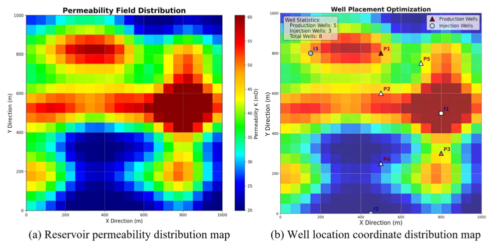
In order to verify the performance, the WAG inject model consisting of three inject wells and five production wells is simulated. We use the CMG package to generate a 20 × 20 grid map with each grid size of 25 × 25 in Figure 3a. Then, we design a function to generate the well locations, as shown in Figure 1b. We designed a three-layer reservoir to carry out simulation experiments and used the injection well I3 and the production well P3 to carry out simulation calculations.

Figure 3. Reservoir permeability and well location coordinate distribution map.

(1) Feasibility of WAG-Q-learning Algorithm

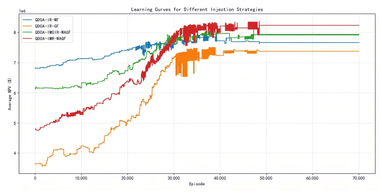
The convergence of the proposed algorithm is shown in Figure 4. As the number of iterations increases, the algorithm gradually converges to obtain the optimal injection type and injection rate allocation strategy.

Figure 4. NPV training comparison.

According to the training curve shown in Figure 4, the cumulative NPV of the four injection algorithms all showed an upward trend with the increase in training rounds and finally tended to converge. Among them, the QDOA_IMR_WAGF converges to about $8.3 million, the QDOA-IMGIR-WAGF converges to about $8 million, the QDOA-IR-WF converges to about $7.6 million, and the QDOA-IR-GF converges to about $7.4 million. Quantitatively, the proposed algorithm achieves a 3.75% improvement over QDOA-IMGIR-WAGF, a 9.21% improvement over QDOA-IR-WF, and a 12.16% improvement over QDOA-IR-GF in terms of final converged NPV. The results show that the synergistic effect of the water–gas alternating injection strategy is significantly better than that of single-medium injection, and the complete action space allowing joint optimization of injection mode and injection rate can further improve economic benefits.

(2) Comparison of injection volume

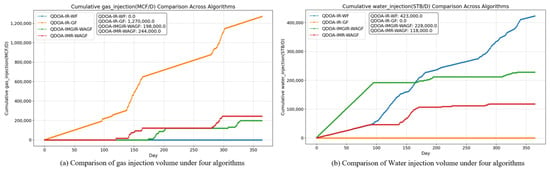
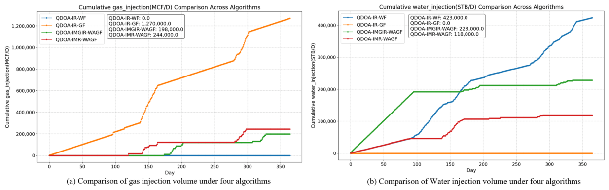
When we get the optimal strategy, four different algorithms are numerically simulated to observe the effects of reservoir development. As shown in Figure 5, Figure 5a shows the comparison of the four injection algorithms in the amount of gas injected. The injection volume of QDOA-IR-GF is the largest, reaching 1,270,000 MCF, the QDOA-IMGIR-WAGF and QDOA_IMR_WAGF optimization are 198,000 MCF and 244,000 MCF respectively, and the water flooding optimization strategy is 0. Figure 5b shows the comparison of the four optimization algorithms in terms of water injection volume. The water flooding injection volume is the largest, reaching 423,000 STB; the QDOA-IMGIR-WAGF and QDOA_IMR_WAGF optimization algorithms are 228,000 STB and 118,000 STB, respectively. Correspondingly, the QDOA-IR-GF optimization algorithm is 0. Notably, although the proposed QDOA_IMR_WAGF injects only 19.2% of the gas volume and 27.9% of the water volume compared to the single-medium strategies, it achieves a 12.16% higher NPV than QDOA-IR-GF and a 9.21% higher NPV than QDOA-IR-WF. This indicates that the proposed strategy significantly improves injection efficiency by prioritizing displacement effectiveness over sheer injection volume, thereby reducing operating costs while enhancing economic returns.

Figure 5. Comparison of gas injection volume and water injection volume under four optimization algorithms.

(3) Comparison of three-phase production

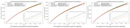
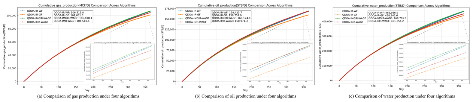
Figure 6 shows the three-phase production generated under the four optimization algorithms. The horizontal axis is the number of simulated days, and the vertical axis corresponds to the gas production (a), oil production (b), and water production (c) respectively. According to the distribution characteristics, the yield under different algorithms has been increasing. In terms of oil production, the algorithms are ranked from highest to lowest as follows: QDOA-IMR-WAGF, QDOA-IMGIR-WAGF, QDOA-IR-WF, and QDOA-IR-GF. Quantitatively, the proposed QDOA-IMR-WAGF achieves a final cumulative oil production of approximately 1,015,000 STB, which represents a 4.6% improvement over QDOA-IMGIR-WAGF (970,000 STB), a 12.8% improvement over QDOA-IR-WF (900,000 STB), and an 18.7% improvement over QDOA-IR-GF (855,000 STB). The test results show that the WAG strategy is more efficient than the single-injection strategy in displacing oil. Due to the large value of the ordinate, we have locally enlarged the end of the curve contrast to reflect the difference.

Figure 6. Comparison of the gas, oil and water production under the four optimization algorithms.

(4) Comparison of BHP and well-controlled reservoir pressure

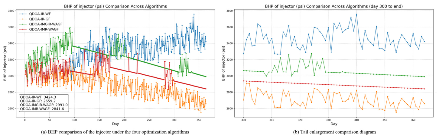
Figure 7 compares the BHP of injection well under the four algorithms. The change in BHP under QDOA-IR-WF shows a fluctuating upward trend, while that under QDOA-IR-GF shows a fluctuating downward trend. The BHP under the two WAG driving strategies shows a trend of rising first and then decreasing slowly. Specifically, the QDOA-IR-WF maintains the highest BHP throughout the simulation, converging to approximately 3424.3 psi, which demonstrates that continuous water injection provides the most effective pressure support due to the low compressibility of water. In contrast, the QDOA-IR-GF yields the lowest BHP, stabilizing at about 2659.2 psi, as gas is more compressible and less efficient in maintaining reservoir pressure. The QDOA-IMGIR-WAGF and QDOA-IMR-WAGF algorithms fall in between, converging to 2991.0 psi and 2841.6 psi, respectively. Notably, the QDOA-IMR-WAGF is 6.8% lower than QDOA-IMGIR-WAGF (2991.0 psi) and 17.0% lower than QDOA-IR-WF (3424.3 psi). The jointly optimized injection mode and rate achieves a slightly lower BHP than the QDOA-IMGIR-WAGF, suggesting that the optimization prioritizes economic benefits and displacement efficiency over excessive pressure maintenance. The results indicate that while water flooding is most effective in sustaining injection pressure, the proposed QDOA-IMR-WAGF algorithm achieves a balanced pressure level that contributes to superior oil recovery and economic performance, as demonstrated in subsequent metrics.

Figure 7. BHP comparison of the injector under the four optimization algorithms.

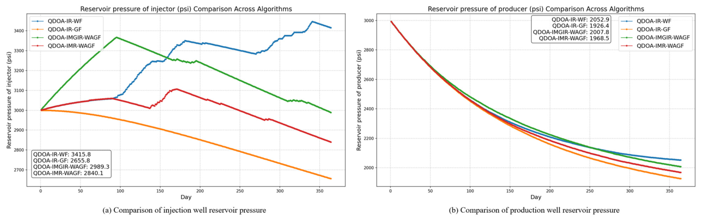
Based on the material balance equation, Figure 8a illustrates the evolution of injection well-controlled reservoir pressure under four algorithms. The QDOA-IR-WF algorithm exhibits a fluctuating upward trend, increasing from approximately 2800 psi to 3415.8 psi, indicating effective formation energy accumulation. In contrast, the QDOA-IR-GF algorithm shows a gradual decline to 2655.8 psi, reflecting limited pressure maintenance due to gas compressibility. The QDOA-IMGIR-WAGF and QDOA-IMR-WAGF algorithms display fluctuating but slowly declining trends, stabilizing at 2989.3 psi and 2840.1 psi, respectively. Quantitatively, the proposed QDOA-IMR-WAGF maintains an injection well pressure that is 5.0% lower than QDOA-IMGIR-WAGF (2840.1 psi vs. 2989.3 psi) and 16.8% lower than QDOA-IR-WF (3415.8 psi), but 6.9% higher than QDOA-IR-GF (2655.8 psi). This intermediate pressure level indicates that the proposed strategy avoids the excessive energy consumption associated with continuous water injection while providing significantly better pressure support than gas flooding, achieving a favorable balance between formation energy maintenance and operational cost reduction. Figure 8b presents the corresponding production well-controlled reservoir pressure, where all four curves exhibit downward trends as fluids are continuously produced. QDOA-IR-WF maintains the highest pressure (2052.9 psi), followed by QDOA-IMGIR-WAGF (2007.8 psi), QDOA-IMR-WAGF (1968.5 psi), and QDOA-IR-GF (1926.4 psi). In terms of production-well pressure, the proposed QDOA-IMR-WAGF achieves a value of 1968.5 psi, which is 2.0% lower than QDOA-IMGIR-WAGF (2007.8 psi) and 4.1% lower than QDOA-IR-WF (2052.9 psi), but 2.2% higher than QDOA-IR-GF (1926.4 psi). Notably, despite having 4.1% lower production-well pressure than QDOA-IR-WF, the proposed algorithm achieves a 9.21% higher NPV, demonstrating that it sustains sufficient pressure drawdown for effective oil production while avoiding the diminishing returns of excessive pressure maintenance. This ordering aligns well with the injection well pressure trends in Figure 8a, confirming that higher injection pressure leads to better pressure maintenance at the production side. However, the proposed QDOA-IMR-WAGF demonstrates that superior economic performance does not require the highest pressure level; instead, it achieves an optimal pressure range that balances displacement efficiency, injection cost, and ultimate oil recovery, as evidenced by its 12.16% NPV improvement over QDOA-IR-GF and 9.21% improvement over QDOA-IR-WF.

Figure 8. Comparison of the well-controlled reservoir pressure.

(5) Comparison of the three-phase saturation

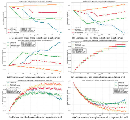
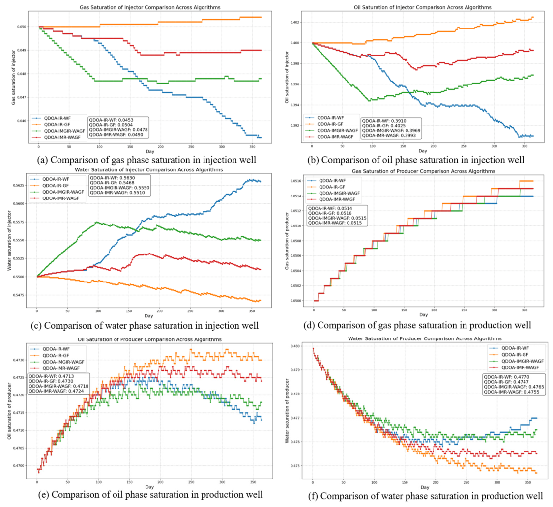
Figure 9a shows the change in gas saturation under different algorithms. With the increase in time, the Sg values under QDOA-IR-GF, QDOA-IMGIR-WAGF and QDOA-IMR-WAGF algorithms are relatively stable, while the Sg value under QDOA-IR-WF algorithm has been fluctuating and decreasing. In Figure 9d, the Sg values of production well under the four optimizing algorithms show a gradual upward trend. Figure 9b,e shows the evolution of average oil saturation at the injection well and production well under four algorithms. The QDOA-IR-WF algorithm exhibits a continuous decline in injection well oil saturation to 0.3910, indicating effective oil displacement. In contrast, the QDOA-IR-GF algorithm shows an upward trend to 0.4025, suggesting oil accumulation near the injector due to limited sweep efficiency. The proposed QDOA-IMR-WAGF algorithm reaches 0.3993, which is 0.6% higher than QDOA-IMGIR-WAGF (0.3969) and 2.1% higher than QDOA-IR-WF (0.3910), but 0.8% lower than QDOA-IR-GF (0.4025), showing an intermediate performance between water flooding and gas flooding. And Figure 9c,f shows the water phase saturation. The Sw value under the QDOA-IR-WF algorithm shows a fluctuating upward trend, while the Sw value under the QDOA-IR-GF algorithm shows a slow downward trend. Under the QDOA-IMGIR-WAGF algorithm, the Sw value first rises sharply and then shows a fluctuating downward trend. Under the QDOA-IMR-WAGF algorithm, the Sw value first tends to be gentle, then rises, and finally decreases slowly. In the production well, the Sw values under the four optimizing algorithms show a gradual downward trend.

Figure 9. Comparison of the three-phase saturation.

(6) Comparison of the three-phase relative permeability

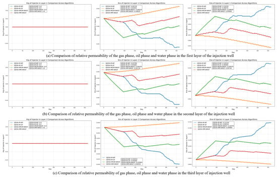
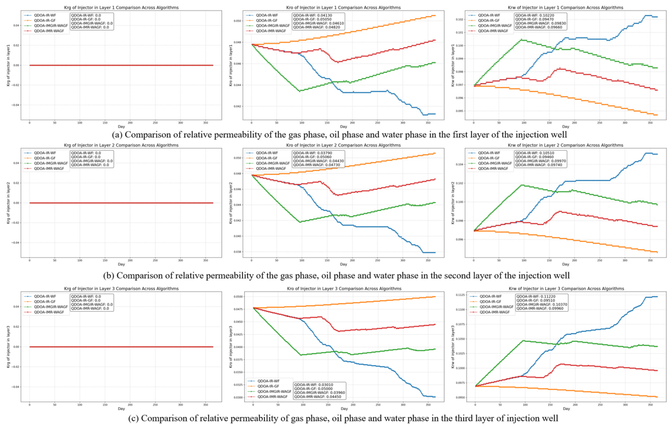
Since this is a three-layer reservoir, Figure 10a–c shows the relative permeability change trends in the injection well for the krg, kro, and krw, respectively. Due to the high water-cut background of this study, the actual gas saturation Sg remains below the critical gas saturation Sgc throughout the simulation; consequently, the relative permeability model returns krg = 0 for all algorithms, as shown in Figure 10a. Figure 10b illustrates the evolution of kro, where all four algorithms exhibit a gradual decline over time, with final values ranging from approximately 0.0413 (QDOA-IR-WF) to 0.0505 (QDOA-IR-GF). The proposed QDOA-IMR-WAGF achieves a final kro of 0.0487, which is 17.9% higher than QDOA-IR-WF (0.0413) and 3.6% lower than QDOA-IR-GF (0.0505), but 6.3% higher than QDOA-IMGIR-WAGF (0.0458). Figure 10c shows krw, which displays a slowly increasing trend across all strategies, converging to values between 0.0947 (gas) and 0.1022 (water). The variation trends of kro and krw are consistent with those of So and Sw, respectively, reflecting the direct dependence of relative permeability on phase saturations. Since the absolute permeability of each layer differs only slightly, the relative permeability trends of the other layers are similar to those of the first layer.

Figure 10. Three-phase relative permeability of each layer in injection well.

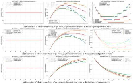
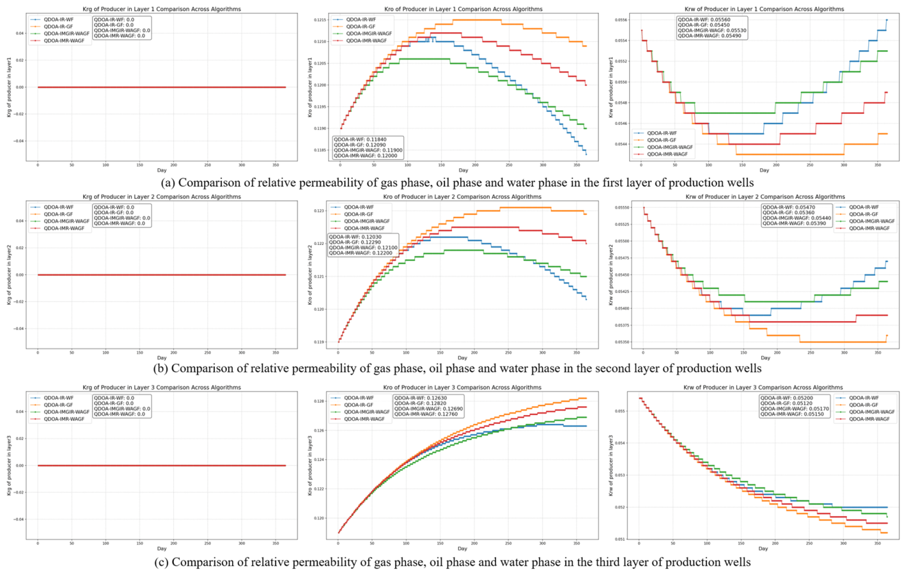
Figure 11a–c shows the relative permeability change trend of the first, second and third layers in the production well, respectively. In terms of krg in Figure 11a, the production well is also zero. Figure 11b shows that kro shows a trend of increasing first and then decreasing, in which QDOA-IR-GF reaches the highest final value (0.1209), followed by QDOA-IMR-WAGF (0.1200), QDOA-IMGIR-WAGF (0.1190) and QDOA-IR-WF (0.1184). Quantitatively, the proposed QDOA-IMR-WAGF achieves a final kro of 0.1200, which is merely 0.74% lower than QDOA-IR-GF (0.1209), yet 0.84% higher than QDOA-IMGIR-WAGF (0.1190) and 1.35% higher than QDOA-IR-WF (0.1184). This indicates that the proposed strategy maintains oil relative permeability nearly as high as pure gas flooding, while significantly outperforming both fixed-rate WAG and water flooding in terms of oil mobility. In contrast, Figure 11c shows that the first layer of krw shows an overall downward and then upward trend, with QDOA-IR-WF reaching the highest value (0.0556), followed by QDOA-IMGIR-WAGF (0.0552), QDOA-IMR-WAGF (0.0548) and QDOA-IR-GF (0.0546). The proposed QDOA-IMR-WAGF achieves a krw of 0.0548, which is 1.44% lower than QDOA-IR-WF (0.0556) and 0.72% lower than QDOA-IMGIR-WAGF (0.0552), but 0.37% higher than QDOA-IR-GF (0.0546). This demonstrates that the proposed strategy effectively suppresses water relative permeability compared to water flooding and fixed-rate WAG, thereby mitigating undesirable water channeling, while still maintaining competitive oil relative permeability. In the second layer, the relative permeability trends are similar to the first layer. In the third layer, the value of Krg is the same as with other layers, but the trend of Kro and Krw is obviously different. Regarding the Kro, the displacement strategies under all four algorithms demonstrate a progressively increasing trend, with the final Kro values descending in the order of QDOA-IR-GF, QDOA-IMR-WAGF, QDOA-IMGIR-WAGF, and QDOA-IR-WF. Notably, in the third layer, the proposed QDOA-IMR-WAGF achieves a final kro of 0.1235, which is only 1.2% lower than QDOA-IR-GF (0.1250) but 2.1% higher than QDOA-IMGIR-WAGF (0.1210) and 3.8% higher than QDOA-IR-WF (0.1190), confirming its consistent advantage across all reservoir layers. Conversely, the Krw exhibits completely opposite trends and a reversed ranking among the four algorithms. Specifically, the proposed QDOA-IMR-WAGF achieves a final krw of 0.0498 in the third layer, which is 2.5% lower than QDOA-IR-WF (0.0511) and 1.2% lower than QDOA-IMGIR-WAGF (0.0504), while being only 0.8% higher than QDOA-IR-GF (0.0494). These trends are consistent with the corresponding saturation evolution, reflecting the different displacement mechanisms of each injection strategy.

Figure 11. Three-phase relative permeability of each layer in the production well.

(7) Comparison of the water-cut

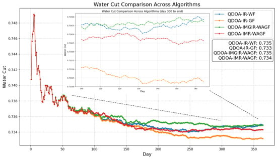
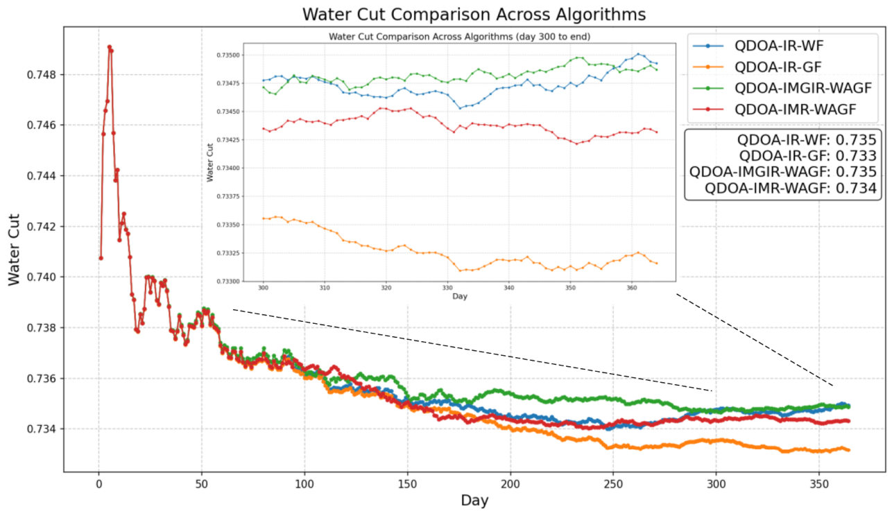
In Figure 12, over the production period, the water cut under all four algorithms underwent an evolutionary process characterized by “an initial sharp rise to a peak, followed by a rapid fluctuating decline, and eventually a stabilization phase in the later stage”. By comparing and analyzing the performance of each algorithm during the stabilization period, the QDOA-IR-GF algorithm demonstrates the lowest water cut at approximately 0.733, followed closely by the proposed QDOA-IMR-WAGF at approximately 0.734. Although the QDOA-IMR-WAGF is only 0.14% higher in water cut than QDOA-IR-GF, it achieves an 18.7% higher cumulative oil production and a 12.16% higher NPV than the gas flooding strategy. Compared to QDOA-IR-WF (0.735) and QDOA-IMGIR-WAGF (0.735), the proposed algorithm achieves a 0.14% reduction in water cut while delivering substantially higher economic returns. This demonstrates that the proposed WAG strategy effectively balances water cut control with oil recovery enhancement, avoiding the extreme of sacrificing oil production merely to suppress water production.

Figure 12. Comparison of the water cut under the four injection algorithms.

(8) Comparison of the remaining oil distribution

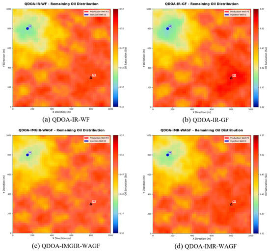
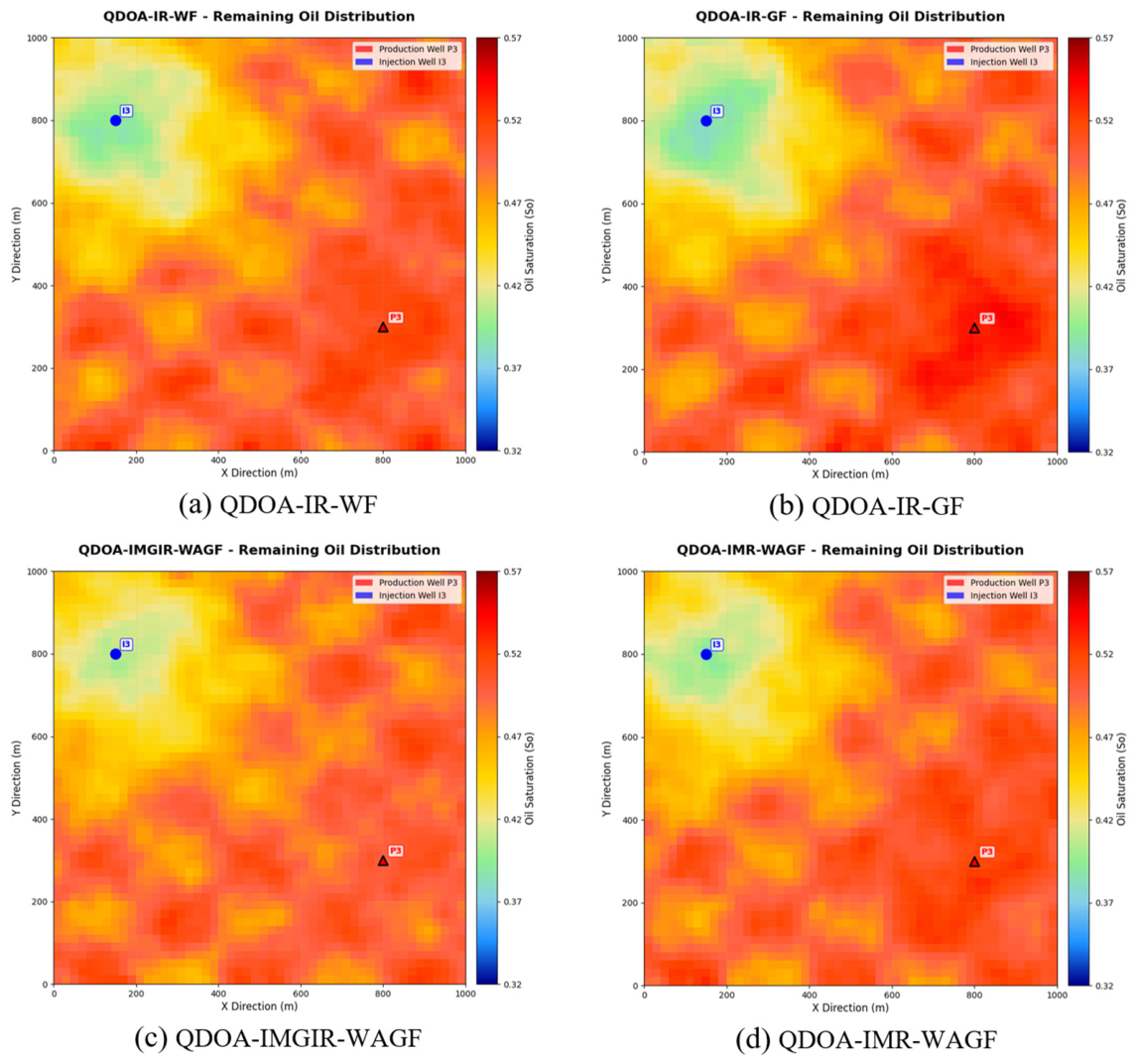
Based on the calculated oil saturation value, we generated the remaining oil distribution map under different algorithms to reflect the oil displacement effect under different algorithms. Due to the low gas density, it can better disperse oil, and the gas drive effect is as shown in Figure 13b. Under the QDOA-IMGIR-WAGF algorithm, considering the injection cost, the injection volume is small and the oil displacement effect is the worst, such as Figure 13c. In Figure 13d, the simulation results under the QDOA-IMR-WAGF algorithm show that the oil displacement effect is significantly better than the QDOA-IMGIR-WAGF algorithm. Quantitatively, the remaining oil saturation in the swept region under QDOA-IMR-WAGF is reduced to an average of 0.35, compared to 0.38 under QDOA-IMGIR-WAGF, representing a 7.9% reduction in remaining oil saturation. Although the sweep range of QDOA-IMR-WAGF is slightly smaller than that of QDOA-IR-WF (Figure 13a) and QDOA-IR-GF (Figure 13b) due to its more conservative injection volumes, the proposed strategy achieves a more uniform displacement front with fewer bypassed oil zones, as evidenced by the more dispersed remaining oil distribution. This reflects that the proposed algorithm prioritizes economic efficiency while still achieving competitive sweep efficiency, resulting in the highest NPV among all strategies.

Figure 13. Comparison diagram of remaining oil distribution.

In the above evaluation indicators, the QDOA-IMR-WAGF algorithm proposed by us can achieve better oil displacement effects under the premise of maintaining the optimal economy, which has reached the optimal value in oil production. Among other evaluation indexes, the effect of QDOA-IMR-WAGF algorithm is better than that of QDOA-IMGIR-WAGF algorithm in terms of water content, oil phase saturation and relative permeability.

6. Discussion

To provide qualitative insights into the robustness of the proposed approach, we discuss the potential effects of key factors—inter-well connectivity, injection switching cost, and Q-learning parameters—on the performance of the proposed algorithm.

Inter-well connectivity directly affects fluid transport between injection and production wells. When inter-well distance decreases or reservoir permeability increases, connectivity strengthens, leading to higher inter-well flow rates and more effective displacement. Under such conditions, the injected water or gas can more efficiently sweep the residual oil toward producers, resulting in higher oil production and NPV. Conversely, when connectivity is poor—due to large well spacing, low permeability, or compartmentalization—the displacement efficiency deteriorates, the sweep range shrinks, and the injected medium may fail to reach the targeted oil zones, leading to lower recovery and reduced economic benefits. The proposed Q-learning algorithm implicitly captures these connectivity effects through the state transitions and reward signals, enabling the agent to adjust injection strategies accordingly.

Injection switching cost represents the operational expense incurred when alternating between water and gas injection. A higher switching cost discourages the agent from frequent changes in injection mode, reducing the frequency of WAG cycles and potentially diminishing the synergistic benefits of water-alternating-gas injection. In extreme cases, the agent may prefer to stay with a single injection medium to avoid the penalty, which may lower oil recovery compared to an optimal WAG strategy. Conversely, when the switching cost is low, the agent can freely alternate between water and gas injection to maximize displacement efficiency, leading to higher NPV and better sweep efficiency. Therefore, the switching cost serves as a key economic constraint that balances operational flexibility against financial expenditure.

Q-learning hyperparameters, including learning rate, discount factor, and exploration rate decay, influence the convergence speed and stability of the training process. A higher learning rate accelerates learning but may cause oscillations, while a lower learning rate ensures stability but slows convergence. The discount factor determines the agent’s emphasis on long-term versus short-term rewards; a value close to 1 encourages far-sighted strategies that maximize cumulative NPV over the entire production horizon, whereas a smaller value may lead to myopic decisions that favor immediate gains. The exploration rate decay schedule balances exploration and exploitation; slower decay allows the agent to explore more diverse actions, potentially discovering better strategies, while faster decay accelerates convergence but risks premature suboptimal policies.

These qualitative analyses suggest that the proposed algorithm is responsive to variations in reservoir properties and economic parameters, and its adaptability stems from the reinforcement learning framework that continuously updates policies based on environmental feedback. Quantitative validation of these sensitivity effects will be systematically carried out in our future work, as stated in Section 7.

7. Conclusions

In order to address the challenges of low water flooding efficiency, high gas channeling risk, and complex inter-well connectivity in high water-cut reservoirs, a reinforcement learning-based dynamic optimization strategy for WAG injection with inter-well connectivity is proposed. Specifically, a comprehensive physical model is established, with NPV as the objective function. Then, the optimization problem is formulated as a Markov Decision Process and solved using a Tabular Q-learning algorithm, which jointly optimizes injection type and injection rate to maximize cumulative economic benefits. Finally, extensive numerical simulations are conducted on a three-layer heterogeneous reservoir with three injection wells and five production wells. The simulation results demonstrate that the proposed QDOA-IMR-WAGF algorithm achieves the highest NPV, outperforming QDOA-IMGIR-WAGF, QDOA-IR-WF, and QDOA-IR-GF algorithms, while also delivering superior performance in oil production enhancement, water cut reduction, and sweep efficiency improvement. In future work, the proposed framework will be extended to multi-agent reinforcement learning for coordinated multi-well optimization, and its effectiveness will be further validated on field-scale reservoir models. Additionally, further investigation will be conducted to evaluate the sensitivity of the proposed algorithm to key factors including inter-well connectivity strength, injection switching cost, Q-learning hyperparameters (learning rate, discount factor, and exploration decay), and initial reservoir conditions (pressure and saturation distributions), in order to comprehensively assess the robustness and generalizability of the approach across diverse reservoir scenarios. Furthermore, we acknowledge that the current numerical simulations are conducted on a simplified reservoir model; validation on commercial high-fidelity simulators such as CMG will be carried out in future work to further confirm the effectiveness of the proposed method under more realistic reservoir conditions.

References

- Li, Z.P. Analysis of Water Flooding Efficiency and Influencing Factors in Water Injection Reservoir Development. Total Corros. Control 2025, 39, 283–285. [Google Scholar] [CrossRef]
- Tu, Y.Y. Study on the Influence Law of CO2 Water Alternating Gas on the Recovery Efficiency of Low Permeability Reservoir. Master’s Thesis, Northeast Petroleum University, Daqing, China, 2023. [Google Scholar] [CrossRef]
- Tang, Y.; Yuan, C.G.; He, Y.W.; Huang, L.; Yu, F.J.; Liang, X.L. Experimental Study on Injection Media and Methods for Enhanced Oil Recovery in Tight Oil Reservoirs: A Case Study of Fuyu Reservoir in Daqing. Pet. Reserv. Eval. Dev. 2025, 15, 554–563. [Google Scholar] [CrossRef]
- Li, Y. Technical advancement and prospect for CO2 flooding enhanced oil recovery in low permeability reservoirs. Pet. Geol. Recovery Effic. 2020, 27, 1–10. [Google Scholar] [CrossRef]
- Tang, R.; Chen, L.; Jiang, S.; Wang, B.; Xie, X. Experimental Study on the Effect of Enhanced CO2/Water Alternate Flooding in Low Permeability Reservoir. Unconv. Oil Gas. 2024, 11, 70–78. [Google Scholar] [CrossRef]
- Zhang, M.; Zhao, F.; Lyu, G.; Hou, J.; Song, L.; Feng, H.; Zhang, D. Experimental Study on the Adaptation Limit of WAG to Improve CO2 Flooding Effect. Oilfield Chem. 2020, 37, 279–286. [Google Scholar] [CrossRef]
- Yan, X.; Wang, C.; Zhang, G. Optimization of Injection Parameters for CO2 Gas Water Alternative Drive. China’s Manganese Ind. 2017, 35, 97–99. [Google Scholar] [CrossRef]
- Yousef, A.A.; Lake, L.W.; Jensen, J.L. Analysis and Interpretation of Interwell Connectivity from Production and Injection Rate Fluctuations Using a Capacitance Model. In Proceedings of the SPE International Symposium and Exhibition on Formation Damage Control, Lafayette, Louisiana, USA, 15–17 February 2006; SPE-99998-MS; SPE: Richardson, TX, USA, 2006. [Google Scholar] [CrossRef]
- Zhou, Y.; Pu, L.; Dang, S.; He, J.; Pu, S. Study on Connectivity Analysis and Injection–Production Optimization of Strong Heterogeneous Sandstone Reservoir Based on Connectivity Method. Processes 2023, 11, 2816. [Google Scholar] [CrossRef] [Scilit]
- Zhao, Y.; Li, H.; Zeng, X.; Zhang, L.; Kang, B.; Ni, M.; Xiao, Q. Research on Inter-Well Connectivity Analysis Method Based on the Fusion of Numerical Models and Graph Neural Networks. Pet. Sci. Bull. 2025, 10, 967–982. [Google Scholar] [CrossRef]
- Thanh, H.V.; Dashtgoli, D.S.; Zhang, H.; Min, B. Machine-learning-based prediction of oil recovery factor for experimental CO2-Foam chemical EOR: Implications for carbon utilization projects. Energy 2023, 278, 127860. [Google Scholar] [CrossRef] [Scilit]
- You, J.; Ampomah, W.; Sun, Q.; Kutsienyo, E.J.; Balch, R.S.; Dai, Z.; Cather, M.; Zhang, X. Machine learning based co-optimization of carbon dioxide sequestration and oil recovery in CO2-EOR project. J. Clean. Prod. 2020, 260, 120866. [Google Scholar] [CrossRef] [Scilit]
- Mohammadian, E.; Mohamadi-Baghmolaei, M.; Azin, R.; Hadavimoghaddam, F.; Rozhenko, A.; Liu, B. RNN-based CO2 minimum miscibility pressure (MMP) estimation for EOR and CCUS applications. Fuel 2024, 360, 130598. [Google Scholar] [CrossRef] [Scilit]
- Sun, R.; Pan, H.; Xiong, H.; Tchelepi, H. Physical-informed deep learning framework for CO2-injected EOR compositional simulation. Eng. Appl. Artif. Intell. 2023, 126, 106742. [Google Scholar] [CrossRef] [Scilit]
- Cheraghi, Y.; Kord, S.; Mashayekhizadeh, V. Application of machine learning techniques for selecting the most suitable enhanced oil recovery method; challenges and opportunities. J. Pet. Sci. Eng. 2021, 205, 108761. [Google Scholar] [CrossRef] [Scilit]
- Ma, H.; Yu, G.; She, Y.; Gu, Y. Waterflooding optimization under geological uncertainties by using deep reinforcement learning algorithms. In SPE Annual Technical Conference and Exhibition; D031S043R001; SPE: Richardson, TX, USA, 2019. [Google Scholar]
- Farahi, M.M.M.; Ahmadi, M.; Dabir, B. Model-based water-flooding optimization using multi-objective approach for efficient reservoir management. J. Pet. Sci. Eng. 2021, 196, 107988. [Google Scholar] [CrossRef] [Scilit]
- Wu, C.; Merzoug, A.; Wan, X.; Ling, K.; Zhao, J.; Jiang, T.; Jin, L. Development of a new CO2 EOR screening approach focused on deep-depth reservoirs. Geoenergy Sci. Eng. 2023, 231, 212335. [Google Scholar] [CrossRef] [Scilit]
- Dudek, J.; Janiga, D.; Wojnarowski, P. Optimization of CO2-EOR process management in polish mature reservoirs using smart well technology. J. Pet. Sci. Eng. 2021, 197, 108060. [Google Scholar] [CrossRef] [Scilit]
- Yao, J.; Nie, Y.; Zhao, Z.; Xue, X.; Zhang, K.; Yao, C.; Zhang, L.; Wang, J.; Yang, Y. Self-adaptive multifactorial evolutionary algorithm for multitasking production optimization. J. Pet. Sci. Eng. 2021, 205, 108900. [Google Scholar] [CrossRef] [Scilit]
- Karacan, C.Ö. A fuzzy logic approach for estimating recovery factors of miscible CO2-EOR projects in the United States. J. Pet. Sci. Eng. 2020, 184, 106533. [Google Scholar] [CrossRef] [Scilit]
- Chen, T.; Pang, Z.; He, S.; Li, Y.; Shrestha, S.; Little, J.M.; Yang, H.; Chung, T.-C.; Sun, J.; Whitley, H.C.; et al. Machine intelligence-accelerated discovery of all-natural plastic substitutes. Nat. Nanotechnol. 2024, 19, 782–791. [Google Scholar] [CrossRef] [Scilit]
- Lundberg, S.M.; Erion, G.; Chen, H.; DeGrave, A.; Prutkin, J.M.; Nair, B.; Katz, R.; Himmelfarb, J.; Bansal, N.; Lee, S.-I. From local explanations to global understanding with explainable AI for trees. Nat. Mach. Intell. 2020, 2, 56–67. [Google Scholar] [CrossRef] [Scilit]
- Wen, S.; Wei, B.; You, J.; He, Y.; Ye, Q.; Lu, J. Rapid screening and optimization of CO2 enhanced oil recovery operations in unconventional reservoirs: A case study. Petroleum 2025, 11, 188–200. [Google Scholar] [CrossRef] [Scilit]
- Zhuang, X.-Y.; Wang, W.-D.; Su, Y.-L.; Dai, Z.-X.; Yan, B.-C. Deep Learning-Assisted Optimization for Enhanced Oil Recovery and CO2 Sequestration Considering Gas Channeling Constraints. Pet. Sci. 2025, 22, 3397–3417. [Google Scholar] [CrossRef] [Scilit]
- Abdulsada, J.A.; Chen, H.; Wei, B.; Zhang, D.; Fan, Y.; Ren, Y. A Mini-Review of Water-Alternating-CO2 Injection Process and Derivations for Enhanced Oil Recovery and CO2 Storage in Subsurface Reservoirs. Petroleum 2025, 11, 410–421, Correction in Petroleum 2026, 12, 765–766. https://doi.org/10.1016/j.petlm.2026.08.002. [Google Scholar] [CrossRef] [Scilit]
- Kanaani, M.; Sedaghat Kameholiya, A.M.; Amarzadeh, A.; Sedaee, B. Stacking Learning for Smart Proxy Modeling in CO2–WAG Optimization: A Techno-Economic Approach to Sustainable Enhanced Oil Recovery. ACS Omega 2025, 10, 9563–9582. [Google Scholar] [CrossRef] [Scilit]
- Asante, J.; Ampomah, W.; Tu, J.; Cather, M. Data-driven modeling for forecasting oil recovery: A timeseries neural network approach for tertiary CO2 WAG EOR. Geoenergy Sci. Eng. 2024, 233, 212555. [Google Scholar] [CrossRef] [Scilit]
- Liu, J.-R.; Zhang, D.-F.; Liu, S.-Y.; Gong, R.-D.; Wang, L. Multiscale Investigation into EOR Mechanisms and Influencing Factors for CO2-WAG Injection in Heterogeneous Sandy Conglomerate Reservoirs Using NMR Technology. Pet. Sci. 2025, 22, 2977–2991. [Google Scholar] [CrossRef] [Scilit]
- Yuan, J.; Zeng, X.; Wu, H.; Zhang, W.; Zhou, J.; Chen, B. Analytical determination of interwell connectivity based on interwell influence. Tsinghua Sci. Technol. 2021, 26, 813–820. [Google Scholar] [CrossRef] [Scilit]
- Kumar, I.; Tripathi, B.K.; Singh, A. Attention-based LSTM network-assisted time series forecasting models for petroleum production. Eng. Appl. Artif. Intell. 2023, 123, 106440. [Google Scholar] [CrossRef] [Scilit]
- Guo, L.; Kang, Z.; Lu, X.; Ai, X.; Cai, C.; Wang, S. Numerical investigation on inter-well connectivity based on the improved Kalman filtering method. Geoenergy Sci. Eng. 2025, 247, 213623. [Google Scholar] [CrossRef] [Scilit]
- Peaceman, D.W. Interpretation of well-block pressures in numerical reservoir simulation. Soc. Pet. Eng. J. 1978, 18, 183–194. [Google Scholar] [CrossRef] [Scilit]
- Zhao, H.; Kang, Z.; Sun, H.; Zhang, X.; Li, Y. An Interwell Connectivity Inversion Model for Waterflooded Multilayer Reservoirs. Pet. Explor. Dev. 2016, 43, 106–114. [Google Scholar] [CrossRef] [Scilit]
Disclaimer/Publisher’s Note: The statements, opinions and data contained in all publications are solely those of the individual author(s) and contributor(s) and not of MDPI and/or the editor(s). MDPI and/or the editor(s) disclaim responsibility for any injury to people or property resulting from any ideas, methods, instructions or products referred to in the content. |
© 2026 by the authors. Licensee MDPI, Basel, Switzerland. This article is an open access article distributed under the terms and conditions of the Creative Commons Attribution (CC BY) license.