


Abstract
An understanding of vortex formation in stirred tank reactors is of great importance, as in some processes, vortices are necessary for a chemical reaction to take place at all or to be accelerated, whilst in other processes, vortex formation is undesirable and can cause high mechanical stresses on the stirrer shaft, sealing and motor drive unit, or may cause undesirable surface aeration or foaming. To gain a better understanding of vortex formation, various baffle systems with different geometries are being experimentally investigated concerning power consumption and the resulting vortices on a single-stage Rushton turbine setup. The shapes of the resulting vortices are described mathematically in terms of vortex depth, width and volume, and the stirring systems prone to vortex formation are simulated using a CFD model based on the Lattice Boltzmann method. The CFD data obtained are compared, validated and verified against the experimental results in order to ultimately be able to fully describe, model and predict vortex formation through simulation. Furthermore, based on the detailed CFD data, vortex formation can be directly correlated with the swirl number, offering a mechanistic characterization method for the vortex shape in various mixing vessel configurations.
1. Introduction
The occurrence of vortex formation in stirred mixing processes presents both a potential danger and an opportunity, posing a challenge for many process experts and operators striving to achieve optimal process performance for a wide range of applications. A vortex in stirred tank reactors is caused by a strong tangential liquid rotation with deformation of the liquid surface, especially when driven by radially pumping impellers. These vortices are often observed with centrally arranged stirrers without baffles (see Figure 1a). However, they also occur when the agitators are positioned off-center or to the side. Vortices are advantageous in some technical applications, such as surface aeration (gassing), foam control, handling emulsions, or suspending poorly wettable floating solids of low density. In unbaffled stirred reactor systems, the power requirement is reduced compared to baffled systems, which can save energy, which in turn can be desirable in large-scale mixing processes. This, however, is counteracted by the risk of an increased tendency for vortex formation, which is why the interplay between power input and vortex depth needs to be addressed during process design [1,2,3,4,5,6].
Except for gasification processes, a crucial disadvantage of vortex formation is the occurrence of highly increased surface aeration as soon as the vortex depth reaches the stirring element. Large amounts of gas are then introduced, which is undesirable for, e.g., homogeneous reactions, heat transfer, or biological cell suspensions. In addition, the stirrer then works partially in air, which means that the stirrer shaft, sealings, bearings and motor drive unit are exposed to vibrations and high mechanical stress. Another aspect is that vortices interfere with the filling level measurements because they increase the level at the tank wall significantly, which makes it difficult to measure the exact filling level [7,8,9].
To minimize or avoid vortices, which are required for most stirring processes, baffles are used in stirred tank reactors (see Figure 1b). These baffles intensify mixing, reduce the tangential flow component of the stirrer, and increase the radial and axial flow proportion by redirecting the tangential main flow, thereby reducing the mixing-inhibiting and vortex-promoting liquid rotation [7,8,10].
Figure 1.
Schematic of a stirred tank reactor. (a) Left: Without baffle and with vortex. (b) Right: With baffles and without vortex [11].
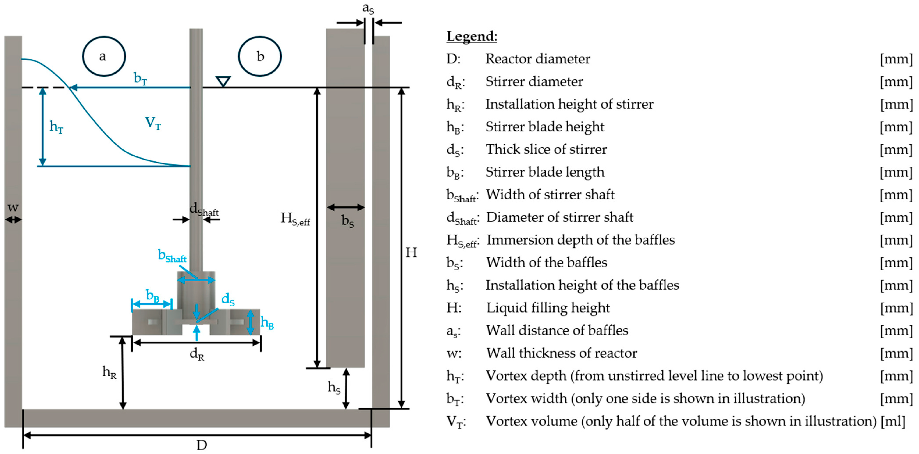
In order to classify a stirred system as unbaffled (vortex formation), partially baffled (formation of unsteady lateral vortex), or baffled (strong surface turbulence but no relevant vortex), the dimensionless baffle index (BW) according to Liepe can be used [12] (see Equation (1); for definitions, see Figure 1).
To reach a fully baffled stirring system, this dimensionless number, which depends on the number of baffles (N) and the geometry (bS, HS,eff and shape factor cF) of the baffles, as well as on the inner diameter of the reactor (D), should be greater than the fully baffled number of the stirrer (BWvb), which, according to Liepe [12], depends on stirrer diameter (dR), inner diameter of the reactor (D), and the dimensionless Newton number (Ne). It is defined as follows (see Equation (2)):
Both indices (BW, BWvb; Equations (1) and (2)) only apply to single-stage stirring systems with H = D = 1 [12]; an analogous description for multi-stage stirring systems is not yet available in the literature. For single-stage stirring systems, a fully baffled state is described in the literature [7,8] with four baffles and the baffles having a width (bS) of D/10 and a wall distance (aS) of D/50. Another fully baffled system is described by Liepe [12] when BW > 0.2.
How to accomplish the fully baffled state with different numbers of baffles has already been analyzed by Heyter and Wollny [10]. The exact prediction of the appearance of vortices, by a mathematical criterion, has not been reported in the literature to date. However, there are already a large number of publications on vortices created with stirrers in systems of different viscosity without baffles [4,9,13,14,15,16,17]. Scargiali et al. [15] not only analyzed the vortices without baffles in differently viscous systems, but also the power characteristic of the systems as a measure for assessing the energy consumption of the connected mixing process. Clark et al. [17] investigated vortex formation and power characteristics in systems with baffles. They found that the power input of reactors using baffles decreases as soon as the surface gassing increases significantly. As of today, the latest literature on vortices and their geometries in stirred reactors with baffles is limited and consists almost exclusively of investigations from the research group of Schultz [11,18,19,20,21].
There are several unvalidated and unverified publications on computational investigations of vortex formation without baffles and with baffles [22,23,24,25], and several publications on simulations that are confirmed by experimental data [2,26,27,28,29,30]. A publication by Zhang et al. [29] should be emphasized, in which investigations of both baffled and unbaffled systems were carried out.
The aim of this study is to fully describe, map, and predict vortex formation and to provide a sustainable and comprehensive approach to the mathematical description of the formation and appearance of the vortices in single-stage stirring processes, with and without baffles, by coupling experiments with CFD simulations. By establishing a CFD model that is validated and verified by experiments, the model can be used to rapidly obtain results for the prediction of the appearance of vortices, thereby minimizing the experimental effort. This investigation represents a feasibility study with two specific objectives. First, new, important correlations for stirring technology and design information for unbaffled and baffled systems should be established and, if possible, compared with the output of previous publications. Second, the applicability of a CFD model based on the Lattice Boltzmann method (LBM) to predict the vortex formation behavior of the two-phase stirring system should be assessed. For this purpose, a comparison will be made between experimental and simulation data. The verified and validated simulation should then be used to reduce the experimental effort, and thus, the advantages of the LBM in terms of reduced computing times compared to conventional simulation approaches should be utilized.
2. Materials and Methods
As this work consists of two parts (experimental and simulation investigations), these are described separately in detail below. The evaluation to describe the vortex depth, width and volume is carried out according to a standardized scheme for both investigation types. The results for the vortices obtained from experiment and simulation are subsequently compared.
2.1. Experimental Setup and Measurement
The experimental measurements are carried out in a laboratory flat-bottom reactor made of transparent polymethylmethacrylate (PMMA; KUS-Kunststofftechnik, Recklinghausen, Germany) with water at 22 °C (ρ = 998.21 kg/m3 [31], υ = 1.003∙10−6 m2/s [31]) as the fluid. The following dimensions of the reactor systems are used (see Table 1).
Table 1.
Dimensions of the used reactor, stirrer and baffles.
A 3D-printed single-stage 6-blade Rushton turbine (RT) [11,33] is used as the stirrer, without baffles and with 3D-printed rectangular (cF = 1 [34]) and cylindrical (cF = 0.45 [34]) baffles, each with two different width dimensions (see Table 1). This results in the baffle index numbers for the different baffle types, based on Equation (1) and Table 1, shown in Table 2.
Table 2.
Baffle index number of the used baffles.
By adjusting the widths of the geometrically adjusted baffles, the rectangular geometry-adjusted baffle index has the same value as that of the cylindrical DIN baffles (see Table 2), while the rectangular DIN baffles have the same baffle index as the cylindrical geometry-adjusted baffles. According to the literature [7,8,12], this means that stirred tank reactors with rectangular DIN and cylindrical geometry-adjusted baffles are theoretically characterized as fully baffled and are supposed to not generate vortices when an averaged Ne number of 5 from the literature [7,8,12,34,35,36,37,38,39] is assumed for the stirrer (BWvb = 0.205). However, the calculated values shown in Table 2 also indicate that in the case of cylindrical DIN baffles and rectangular geometry-adjusted baffles, the systems are theoretically not sufficiently baffled, which means that vortices can be expected. In this case, the influence of baffle geometry on vortex formation becomes apparent.
In order to be able to recognize and metrologically detect possible vortices as a whole, the surface of the baffles is grinded and then painted with clear coat (see Figure 2 left image). Furthermore, to ensure that the baffles are at the same height and do not move during the investigations, they are installed on a three-stage holder using rivet body. The holder also ensures that the stirrer is always installed centrally, because the stirrer shaft is inserted via the center of the holder by three ball bearings. Of course, the holder construction itself is not immersed in the liquid phase [11,21].
Figure 2.
Used baffles. (Left image): (a) Rectangular baffle. (b) Cylindrical baffle. (c) Rectangular geometry-adjusted baffle. (d) Cylindrical geometry-adjusted baffle. (Right image): Experimental setup. (a) Camera. (b) Aquarium with reactor, baffles and stirrer. (c) Torque measuring device. (d) Stirring motor. (e) LED. (f) Computer for power recording. (g) Exemplary vortex with six cylindrical baffles at ReR = 16,800. (h) Exemplary torque measurement [20].
The experimental setup is shown on the right in Figure 2. This setup is used to measure the power input and any vortices that may form. The vortices are illuminated with an LED (Veritas Truth in Light, Pasadena, CA, USA) and recorded as video using a camera (Canon EOS 600D with a Canon EF-S 18–55 mm F3.5–5.6 IS II 58 mm lens, Tokyo, Japan). The measurement duration for the analysis of vortices is 8 s (24 frames per second). From these 8 s, 4 frames are analyzed using the evaluation method described in Section 2.4 [11,21].
The power input is measured using the T22 torque measuring shaft from Hottinger Brüel & Kjaer GmbH (Darmstadt, Germany) (measurement accuracy 0.5%), which is positioned between the stirrer motor (“Microstar 7.5 digital” from IKA-Werke GmbH & CO. KG (Staufen im Breisgau, Germany), range 50 to 2000 rpm) and the stirrer shaft. The measurement is performed in 50 rpm steps until gas entry becomes visible. Each torque measurement generates 3000 values within 30 s, which are converted into power or a Newton value according to Section 2.3 [11,21].
More detailed information on the experimental method can be found in [11,21].
2.2. Simulation
In order to optimize the computing time while maintaining the exact physical model formation and, in particular, taking into account the multi-phase flow and phase interaction phenomena relevant for vortex considerations, a GPU-native Lattice Boltzmann method (LBM) solver is used. The simulations in this study were carried out with the commercially available LBM software SimVantage® (version May 2025). This method was initially developed from lattice gas automata [40]. The regular and equally distant calculation node distribution is typical for LBM and mitigates the effort to create a customized mesh for every geometry. On each of the calculation nodes, 27 distribution functions (fα) with an assigned discretized velocity vector (, Equation (3) for the D3Q27 stencil, which ensures discrete Hermite orthogonality, which is essential for exact modeling) indicate the probability that the fluid mass in the current cell moves in the respective direction α. To compensate for the different orientations of the vectors, weighting factors (wα, Equation (4), for the D3Q27 stencil) are introduced.
A time step in the Lattice Boltzmann algorithm consists of two parts. In the first part, the collision step, an equilibrium distribution function is calculated based on the macroscopic fluid velocity in the cell (Equation (4)). This equilibrium distribution function is then subtracted from the current distribution function and divided by the relaxation factor τ, which depends on the viscosity ν of the fluid. This part of the collision step, including the formulation for the equilibrium distribution function, is called the BGK (Bhatnagar–Gross–Krook) approximation [41].
The collision step is completed by adding the external forces Fα, accounting for the body force density using the formulation of Guo [42] (Equation (6)). The collision step is described in the right-hand side of the main LBM equation (cf. Equation (3)). The left-hand side of the main equation is called the streaming step, which is the second part of the Lattice Boltzmann algorithm. In this step, the resulting distribution functions are transported to the next node in the direction of the respective spatial unit vector. At the end of this streaming step, each node should be equipped with a full set of 27 streamed distribution vectors.
For the simulation of free surfaces, an LBM-Volume of Fluid (VoF) model is implemented first, as proposed by [43], used in many applications [44,45,46], and further enhanced by Anderl et al. [47] to provide a more accurate representation of submerged bubbles. The general idea behind this Eulerian modeling approach is to differentiate the numerical grid between liquid cells, gas cells and interface cells. In liquid cells, the fluid flow calculation is carried out in the usual LBM manner. In gas phase cells, the fluid flow is neglected, and the influence of internal circulation inside the gas bubble is assumed to be insignificant on the liquid flow field, which is justified by the large density differences between the gas and liquid phase. Interface nodes are treated as fluid nodes with an additional boundary condition to recover the distribution functions from the gas phase.
In each grid cell, two new arrays are defined, namely the local liquid volume fraction φ and the local liquid mass m. The liquid volume fraction in liquid cells is defined as 1, whereas gas cells always have a liquid volume fraction of 0. In interface cells, the liquid volume fraction is between 0 and 1. In LBM, the local numerical density varies according to the local pressure. Therefore, the conversion between liquid volume fraction and liquid mass is based on the local fluid density and stored in a separate array (see Equation (7)).
m = φ(Δx)3ρ,
The advection of liquid mass in interface cells and the subsequent movement of the gas-liquid interface is modeled via an advection equation described by Anderl, whereas mass transport to and from gas cells is excluded [47] (see Equation (8)).
In each LBM time step, the individual contributions to the advection of liquid mass are summed up on each interface cell to obtain an updated local liquid mass, which is then converted to the local liquid volume fraction according to Equation (7). If the updated volume fraction is below 0, the interface cell is converted to a gas cell and neighboring nodes are marked as interface cells. To avoid step-by-step fluctuations, a numerical threshold of 0.001 is set for these thresholds, similar to previous studies [48]. Subsequently, interface cells with a volume fraction above 1 are marked as liquid nodes, and neighboring gas nodes are marked as interface cells. With this method, the interface is always ensured to be of thickness 1 in terms of grid size. When former gas cells are newly flagged as interface cells, they do not contain a valid set of distribution functions since gas phase cells are excluded from the liquid calculation. In these cells, the fluid velocity and density of neighboring interface and liquid cells is locally averaged. These average macroscopic quantities are then used to calculate a set of distribution functions according to the equilibrium distribution.
The interface boundary condition is given by Equation (9), where α and denote opposing distribution functions [47]. Since the gas cells are excluded from the fluid calculation, the macroscopic density inside the bubble is not available directly but is modeled from the pressure at the boundary. The pressure term consists of two parts.
The first term pV describes the internal pressure of the bubble (see Equation (12)). In the classical LBM-VoF or Free-Surface LBM model, this term is defined as the atmospheric pressure p0. This assumption is valid for free-surface flows without submerged bubbles only. For submerged bubbles, the classical Free-Surface LBM model does not account for the local pressure gradient surrounding the bubble, which leads to unphysical behavior due to violation of mass conservation. Anderl et al. [47] proposed an enhanced bubble model that tracks the bubble volume throughout the simulation and defines the internal pressure according to the ideal gas law.
The second pressure contribution Δpσ is the Laplace pressure, modeling the pressure difference between the inside and the outside of the bubble based on the local curvature κ(,t) and surface tension σ between the gas and liquid phase (see Equation (13)).
pgas = pV + Δpσ,
In order to determine the local curvature at the interface, several numerical methods are available in the literature, with varying complexity and accuracy. An overview of numerical models for curvature estimation is given by Bogner et al. [49].
In this study, the curvature κ is calculated based on finite differences from the surface unit normal vectors . The surface normal is calculated directly via finite differences from the local filling volume fraction φ.
n = ∇φ,
An additional consideration when modeling droplets or gas bubbles encountering solid surfaces, such as in bioreactors, is the wetting behavior of the liquid phase. Bogner et al. [49] presented a boundary condition at the solid walls to incorporate the contact angle θeq of droplets on a solid surface, which then influences the direction of the surface normal and subsequently the curvature, which influences the behavior of the interface. denotes the surface normal to the solid wall, and denotes a tangential vector at the wall, which is normal to the contact line of the interface (see Equation (16)).
The simulations are carried out with a uniform grid resolution of 0.5 mm, and the time step is based on a fixed tip velocity of 0.05 in lattice units, which results in a time step in the order of 10−5 to 10−4 s in the investigated range of operating conditions. A tip speed of 0.05 lattice units is commonly used in LBM simulations of stirred tank applications to satisfy the Courant–Friedrichs–Lewy criterion. In order to stabilize high Reynolds numbers at relaxation times near 0.5, the Smagorinsky–Lilly model for subgrid-scale modeling of turbulence via large eddy simulation was employed with a Smagorinsky constant of 0.1. The framework and numerical settings used in this manuscript have been validated and compared to PIV measurements in a previous study [50] for single phase systems, where comparisons between different discretization stencils and turbulence models was performed.
2.3. Experimental Evaluation of the Torque Measurement
The measured experimental data obtained from the torque (M) measuring shaft are averaged, and the power input (P) and Newton number (Ne) are calculated using Equations (17) and (18).
P = 2∙π∙M∙n,
To calculate the pure power input per volumetric element, the measured power is divided by the present fluid volume (V). This is called the volume-specific power input (P/V), which is plotted against the Reynolds number (Re) (see Equation (19)).
2.4. Evaluation of the Vortices
The method used to analyze the vortices found in the experiment and simulations follows a standardized identical procedure using Matlab® (version R2022b) macros. The evaluation procedure for the experimental and simulated images is illustrated in Figure 3 using a simulation image as an example.
Figure 3.
Exemplary evaluation of a vortex without baffles at ReR ≈ 6640.
Depressions in the surface of the liquid are classified as vortices if they contain at least 0.1% of the reactor volume [11,21]. Once this volume is reached, measurements are taken only every 100 rpm until gas enters the system. Systems in which the vortex volume determined in the experiment matches the definition are then also taken into account in the corresponding CFD simulation.
The only differences in the analysis methods between the experiment and the simulation are, on the one hand, that videos must be cut for the experiments, whereas in the simulation, the images of the vortices must be set in contrast using Paraview®(version 5.12.0). Furthermore, in the experiment, a calibration image is captured with graph paper, and 70 mm is measured as scale to describe the vortices in millimeters rather than pixels. In the simulation, the scale on the right in the images is used, and a calibration of 50 mm is performed. These differences do not affect the method used to analyze the vortices. Adjusting the contrast of the simulation images is done so that the same Matlab® macro used in the experiments can be applied to detect the vortices in the simulation. The calibration lengths also do not affect the results, since the lengths used are factored into the calculation of the conversion factor.
The vortex images from the experiment and the simulation are imported into Matlab®, and the pixels are converted to millimeters. The images are then cropped, in a first step roughly and then finely at the filling line. Once the vortex is cut out, several different macros are run over the image to smooth the transitions and remove slight imperfections so that the vortex can be clearly detected. Finally, the derived vortex geometry is imported into an x-y diagram [20].
A mathematical vortex description is derived from the data points obtained. Previous experimental runs have shown that the vortices are well described by a fourth-degree polynomial function (see Equation (20)) [11,20,21].
The geometric data of the vortex depth, width and volume are determined from Equation (20) and subsequently referred to the unstirred level line, as described in the literature [8,12,31]. The first derivative of Equation (20) is formed for the vortex depth, as the lowest point of the function is the zero point of the first derivative. This point is then inserted into the polynomial function and the linear function, which is the unstirred level line, and then added together.
To obtain the vortex width, the intersection points of the fourth-degree polynomial function with the unstirred level line are calculated and added together.
The vortex volume is obtained by shifting the vortex curve so that the low point is at (0/0). The rotational formula is then performed while integrating the curve (see Equation (21)).
Detailed descriptions of the analyses can be found in [11].
The results presented in the Section 3 regarding vortex depth, width and volume show the mean values and standard deviations of the means of the four largest vortices (worst-case assessment) found in the quasi-steady state for each rotational frequency. An analysis of more than four vortices does not result in any significant changes, and the use of randomly selected vortices also leads to no significant difference.
2.5. Grid Convergence
A mesh refinement analysis was carried out for three spatial resolutions of 1200, 1600 and 2000 nodes per meter, corresponding to lattice spacings of 0.833, 0.625 and 0.5 mm. For this grid refinement study, the condition with the largest vortex formation was compared, where the largest deviations due to grid sensitivity are expected. For each resolution, the depth, width and volume of the vortex were averaged over four points in time in the quasi-steady state (Figure 4). The refinement ratios of 1.33 and 1.25 are within the recommended ratio of 1.3 by Celik et al. [51]. The change between the two coarser resolutions is considerably larger than between the two finer ones and, for the depth, of the opposite sign. This is partly attributed to the representation of the stirrer blade. Its thickness of 1.5 mm spans only 1.8 cells at 0.833 mm and is therefore only partly resolved, so that the coarse grid cannot recover the full blade geometry. Between the two finer resolutions, the width and volume of the vortex deviate by less than 3%, while the depth deviates by 5%. All results presented below were obtained with 0.5 mm.
Figure 4.
Effect of grid resolution on the simulated vortex depth, width and volume for the unbaffled setup at the highest Reynolds number (Re = 15,703).
3. Results and Discussion
The results of power measurements as well as vortex detection and analysis are presented and discussed below. As the main focus is on the vortices, only the vortex depth, width and volume are compared with the simulation results, so that the experimental power measurements represent valuable additional design information for technical applications. The analyses were carried out using the methods described in Section 2.3 and Section 2.4. In addition, the results are used to illustrate dependencies for the vortex volume, and the fully baffled number for a Rushton turbine is provided.
3.1. Power Measurements and Volume-Specific Power Input
To determine the power characteristics, the respective torque values are recorded for each rotational frequency. Averages, as well as the Newton and Reynolds numbers, are then calculated using Equations (17)–(19). Figure 5 shows, on the left, the power characteristics of the various systems with baffles and without baffles and, on the right, the related volume-specific power input of these systems.
Figure 5.
Experimental results for unbaffled and various baffled systems with six baffles each Rushton turbine; for details see Section 2.1.
Both diagrams show that the cylindrical geometry-adjusted baffles have the highest power input, while the rectangular geometry-adjusted baffles and no baffles deliver the lowest volume-specific power input. A comparison of the two DIN baffles shows that the cylindrical baffles are slightly more energy efficient than the rectangular baffles. Additionally, the correctness of the measurements is also shown qualitatively by the fact that in Figure 5 left image the curves of the pairs of measured values of the rectangular DIN baffles and the cylindrical geometry-adjusted baffles adapted to them (both with BW = 0.325) are very close to one another; similarly, this is true for those of the cylindrical DIN and the rectangular geometry-adjusted baffles (both with BW = 0.146). The lowest Newton number is obtained in the unbaffled system, which is in accordance with previous studies [7,8,15].
If Figure 5 left image is compared with the literature [7,8], it can be seen that the curves agree with published data. This means that without baffles, the power characteristic continuously decreases (∞) with increasing Reynolds number of the stirrer, whereas with baffles in the turbulent region (ReR > 104), the Newton numbers are almost constant.
It can also be seen that the scatter of the values in the power characteristic curves becomes very small with Reynolds numbers from the transition area of around 2000 upwards. Due to the low stirring frequencies and velocities below this transition region, the measuring device with an accuracy of 0.5% per measured value results in higher fluctuations and slightly larger deviations here.
The literature [7,8,12,34,35,36,37,38,39] gives Newton numbers in a range between 3.6 and 6.5 for a Rushton turbine in the turbulent regime. The Newton number determined with the various baffles from the experiment here shows slightly lower Newton numbers for the turbulent regime, except for the rectangular DIN and cylindrical geometry-adjusted baffles (see table in Figure 5, left image). However, it should be noted that, unlike in this paper, in the literature the exact details of the reactor setup used for the measurement, i.e., which liquid was measured with how many baffles and which type, width, wall space and immersion depth of baffles, the installation height of the stirrer, the diameter of the stirrer, and the blade thickness of the stirrer, unfortunately, are often not available. This can lead to the differences shown, as the stirrer sets the liquid in motion with more or less energy, depending on the geometries and viscosities used. In order to increase comparability in future, authors should provide more information in corresponding publications, just as precisely and in detail as in this paper.
With regard to vortex formation, it should be noted that there was no vortex formation with rectangular DIN baffles and cylindrical geometry-adjusted baffles, which is consistent with the theoretical prediction using Liepe’s formula [12], presented in Section 2.1. However, the use of cylindrical geometry-adjusted baffles is not recommended for industry, as they cause high energy consumption and lower productivity due to their width. But they serve as a reference here. In comparison, rectangular DIN baffles need less material, are easier to manufacture, and therefore cheaper; overall, they seem to be more economical and thus more suitable for processes where vortex formation is not permitted. The cylindrical DIN baffles and the rectangular geometry-adjusted baffles show vortex formation; their geometries and baffle number of BW = 0.146 are therefore insufficient for the complete prevention of vortices.
In applications where a vortex is necessary, i.e., applications requiring surface gassing or emulsification, either no baffles (BW = 0) or rectangular geometry-adjusted or cylindrical DIN baffles with a baffle number of 0.146 can be used. In low-viscosity liquids such as water, it can be seen that the formation of a vortex with no baffles or with rectangular geometry-adjusted baffles already occurs in the transition regime at ReR ≈ 4400 or ReR ≈ 6640, respectively. This shows that the rectangular geometry-adjusted baffles, compared to no baffles, initially have an effect of preventing or delaying vortex formation. This effect is further delayed with the cylindrical DIN baffles, so that vortex formation here only occurs in the turbulent regime at ReR ≈ 11,100 and above.
It can be seen that the cylindrical DIN baffles and the rectangular geometry-adjusted baffles, despite having the same baffle number, show a different effect; therefore, baffle type and geometry have a pronounced effect on vortex formation.
3.2. Vortex Depth
Firstly, the depth of the vortices is considered and discussed for the three different stirring systems that form vortices (unbaffled, cylindrical DIN baffles, rectangular geometry-adjusted baffles). In Figure 6, on the left, the vortex depth is plotted against the Froude number (Fr, see Equation (22)), as the Froude number relates centrifugal force and gravity and therefore takes into account the processes at the surface of the liquid and the influence of the gravitational acceleration (g) on the stirring instance [31]. Furthermore, Figure 6, on the right, also shows the vortices in the experiment and in the simulation for the three different stirring systems.
Figure 6.
(Left): Mathematical descriptions of the vortex depth from the experiment and the simulation against the Froude number. (Right): Picture of the vortices in the experiment and simulation at different Reynold numbers. (Top): Unbaffled system. (Middle): System with six cylindrical DIN baffles (BW = 0.146). (Bottom): System with six rectangular geometry-adjusted baffles (BW = 0.146).
As mentioned in Section 3.1, with increasing stirrer speed, vortex formation starts earliest with no baffles and latest with cylindrical DIN baffles. This can be seen from the Froude number in the diagrams of Figure 6. It can also be seen that the vortex depth is highest with no baffle and lowest with the cylindrical baffles at comparable Froude numbers.
For all three different stirring systems, both the experiments and the simulations show that the vortex depth is linearly dependent on the Froude number, which was also found by Zlokarnik [9] for systems without using baffles. The linearized description is very good for all three stirring systems, as can be seen with the coefficient of determination (R2 > 0.97).
A comparison of the three different setups in the experiment and the simulation shows that the vortex depth is least scattered without a baffle, while with baffles there is more scattering, even with an increase in the rotational speed (see error bars in Figure 6). This is because the vortices do not move much without a baffle. With baffles, which are supposed to suppress vortex formation, there is more vortex movement because the baffles break up the tangential flow regime of the stirrer and redirect the flow in axial and radial directions. This inevitably leads to higher fluctuations and turbulence in the flow field, resulting in more vortex movement, as well as greater fluctuations in the description of the vortex depth.
Comparing the linear functions from the experiments with the simulations, in particular the slope factors of these functions, there is a very good match for the case without baffles. In comparison, the value deviates slightly by only about ≈4.9%. As with the error bars, this small tolerance can be explained by the small flow fluctuations and changes or movement of the vortex. When analyzing the two different baffle installations (cylindrical DIN and rectangular geometry-adjusted), there is an expected and slightly larger difference between the experiment and the simulation than in the unbaffled version of the reactor. Nevertheless, the agreement is good for a technical application, given the fact that the simulation model does not use any fitting factors, i.e., it is a first-principles simulation. It should be noted that the first simulation value for the rectangular geometry-adjusted baffles does not reach the given definition of a vortex volume, which is why the result is shown in a different color in the diagram.
Beginning with the rectangular geometry-adjusted baffles, the vortex depth is slightly higher in the experiment than in the simulation. When comparing the slope factor of the derived formulas and correlations from Figure 6 for experiment and simulation, there is a difference of 30.1%. The deviations appear to be acceptable qualitatively with regard to the design of technical applications, especially since vortex width and volume analyzed below show good agreement between experiments and simulations. Quantitatively, however, a deviation of over 20% in the vortex depth directly is deemed insufficient for a direct correlation, which is why, in Section 3.5, the swirl number analysis is derived from the whole flow field from the simulation against the experimental vortex depths. It should be noted here that further increasing the mesh resolution or sampling size did not lead to a better agreement. The residual deviation in the slope of the vortex depth prediction in the rectangular geometry-adjusted setup seems to have a systematic cause, which could not be ruled out by increasing the mesh resolution. Future work in this direction will follow, but it should be noted that the results presented here already show a promising agreement between experiment and simulation, which speaks for the high quality of the experimental methodology and the associated model building strategy. This means that the main task of this feasibility study has already been fulfilled. Besides, the mathematical determination of the vortex depth for the simulation can also be used to determine vortex depths at lower frequencies, so that the simulation provides a very good description of the vortex depth for these baffles.
In contrast, the cylindrical DIN baffles show significantly better agreement between the experiment and simulation. As with the cases without baffles, the deviation is less than 1%. The simulation shows greater fluctuations (see error bars in Figure 6) with cylindrical DIN baffles than with the rectangular geometry-adjusted baffles, so that the simulation values correspond very closely to the experimental values. This indicates that the cylindrical DIN baffles in the simulation are able to reflect reality better than the rectangular geometry-adjusted baffles.
Furthermore, in both the experiment and the simulation of the system under consideration with a Rushton turbine, it can be seen that with a comparable baffle index, the formation of vortices with cylindrical DIN baffles only begins at higher Reynolds numbers. Since the baffle index is the same, this indicates flow effects. Rectangular baffles represent a geometrically “rougher” flow resistance than cylinders, which can be flowed around more smoothly due to their shape. This could lead to more intensive mixing, flow uniformity, and reduced vortex-promoting tangential flow fraction. This assumption is supported based on the observations of the slightly higher Newton numbers and volume-specific power inputs for cylindrical baffles shown in Figure 5.
In order to describe the dependency of vortex depth on the Reynolds number, the dimensionless vortex factor (cT) is often used in the literature [4]. This dimensionless vortex factor is defined as follows (see Equation (23)).
In Figure 7, the vortex factor is plotted against the stirrer Reynolds number for the three different stirrer setups with vortices. It can be seen that the vortex factors without baffles are clearly but expectably higher than those with baffles. Furthermore, as with the plot of the depth of the vortices against the Froude number (see Figure 6), the error bars with baffles in the corresponding plots in Figure 7 are larger than those without baffles. The reason is the same as discussed before and lies in the increased turbulence and fluctuation of the flow due to the disruption of the tangential flow by the baffles.
Figure 7.
Dimensionless vortex factor of the three stirring systems that form vortices as a function of Reynolds number.
When looking at the values without baffles, it is noticeable that they increase up to ReR > 104 and then tend to be constant, which is identical to the findings and results of Markopoulus et al. [4].
The measurements with the cylindrical DIN baffles show a very constant value with increasing stirrer Reynolds number. This observation corresponds to the assumption from above that the cylindrical DIN baffles bring about a significantly better flow uniformity, but at the expense of a slightly increased power input compared to rectangular baffles with the same baffle index.
With the rectangular geometry-adjusted baffles, there is a constant trend for cT between 4.8 ∙ 10−1 and 5.4 ∙ 10−1 for the experiment. The simulation values are again smaller but also show a constant trend with increasing stirrer Reynolds numbers. While vortex volume and width are described within a 20% band to the experiments, the 30% deviation in the vortex depth hints at further refinement necessary in the models to cover a broader range of geometries, which will be addressed in subsequent work.
Nevertheless, an important finding that can be derived from the data is that the constant levels of the dimensionless vortex factors in both the cylindrical DIN and the rectangular geometry-adjusted baffled systems point to the flow-balancing function, which, as a side effect, at least delays the formation of the vortices. The dimensionless vortex factors also show that the rectangular geometry-adjusted baffled system is more susceptible to the formation of a vortex than the cylindrically baffled system with the same baffle index. A comparison of these findings with the literature cannot be done, because in this regard, the literature only contains systems without baffles.
3.3. Vortex Width
As a further geometric description, the vortex width of the three different vortices generating stirring systems is shown and discussed. Figure 8 presents the vortex width plotted against the Froude number on the left and vortex images over three seconds for one stirrer Reynolds number on the right.
Figure 8.
(Left): Mathematical descriptions of the vortex width from the experiment and the simulation. (Right): Picture of the vortices over three seconds with one Reynolds number for the experiment and simulation. (Top): Unbaffled system. (Middle): System with six cylindrical DIN baffles (BW = 0.146). (Bottom): System with six rectangular geometry-adjusted baffles (BW = 0.146).
As visible in Figure 8, an interesting finding is that, unlike the vortex depth, which clearly increases linearly with the Froude number and is only limited when the vortex reaches the stirring element, the vortex width has a more logarithmic progression depending on the Froude number. This suggests that the vortex width increases strongly with increasing stirrer rotation speed and Froude number, but then reaches an almost constant final value from Fr = 0.1 for the unbaffled system or Fr = 0.4 for the rectangular baffled system and Fr = 0.5 for the cylindrically baffled system. These logarithmic functions can only be assumed if the vortices have a width above D/10 [11,21].
In general, and in contrast to the vortex depth described in Section 3.2, there seems to be a slight tendency for the vortex width to be higher for the simulation values than those measured experimentally.
For the unbaffled system, the error bars in the experiment are smaller than in the simulation. In the simulation, the vortices move slightly more in the low Reynolds number/Froude number range than in the experiment. At higher Reynolds numbers, such as 11,100, the images show no significant differences in width for either the experiment or the simulation. Due to the poor logarithmic fit of the vortices in the simulation and the experiment, the slope values of the function between the simulation and the experiment differ by 68.2%. If the errors were added to the results in the experiment and subtracted from them in the simulation, the values would match better, and the deviation would be smaller.
For the stirring systems with baffles, both systems show higher error bars than for the unbaffled stirring system. This can again be explained by the fact that the flow regime is broken up by the baffles used, causing the vortex to move more; see analogous explanation in Section 3.2. This can be seen very clearly in the vortex images next to the diagrams. It should also be noted that only four images are analyzed as snapshots in both (the experimental and simulation) methods, so only parts of the vortex appearance are visible with the values, which can also explain the larger error bars.
The simulated vortex width for the cylindrical DIN baffles is smaller than that observed in the experiment. If the error bars are taken into account, the values from the simulation and the experiment would agree very well. The experimental values, in particular, show a very good logarithmic fit, as the vortices continue to increase with rising Reynolds number/Froude number. In the simulation, however, a very high vortex width is already observed in the first vortex, which then decreases with the Froude number and subsequently increases again, meaning that the vortex width cannot be well described by a logarithmic function.
In the case of the rectangular geometry-adjusted baffles, the experimental values and simulated values match very well, taking the error bars into account. However, the fact that the first vortex (purple) in the simulation does not match the definition of a vortex is disregarded here and not taken into account. This means that the logarithmic function can only be used to describe the data to a limited extent, resulting in a significant deviation of 45.5% between the experimental and simulated slope values.
A comparison with literature values cannot be made at this point, as the vortex width is not considered in the literature so far.
3.4. Vortex Volume
As a final vortex description measure, the vortex volume is presented and discussed. For this purpose, the vortex volumes of the three different mixing systems are plotted against the Froude number in Figure 9 and described mathematically using a linear regression through zero. The coefficients of determination of these regressions are above 0.96 and thus provide a good description of the results for all three stirring systems.
Figure 9.
Mathematical description of the vortex volume without, with cylindrical, and with rectangular geometry-adjusted baffles. (Left): Unbaffled system. (Middle): System with six cylindrical DIN baffles (BW = 0.146). (Right): System with six rectangular geometry-adjusted baffles (BW = 0.146).
In addition, the error bars for the vortex volume are confirmed to be very small for the stirring system without a baffle, as already seen for the vortex depth (see Figure 6) and the vortex width (see Figure 8), which can be attributed to the low vortex fluctuations around the stirrer shaft. The comparison of the slope factors of the linear regression for the mixing system between experiment and simulation is approximately 12.1%, and this slight deviation has also already been reflected in vortex depth. Only the width has larger deviations because of the comparatively poor logarithmic function. This means that the description of the vortex without a baffle can be reproduced well with the CFD model.
With baffles, there is again more scattering in the results due to the many vortex movements (see error bars in Figure 9) caused by the breakup of the stirrer flow regime by the baffles. However, these variations result in a good mathematical fit for cylindrical DIN baffles, so that the slope values of experiment and simulation do not deviate from one another. It is thus evident that the simulation is very well suited for the vortex volume with cylindrical DIN baffles, although there are significant differences in width.
A comparison of the slope factors for the rectangular geometry-adjusted baffles shows that the mathematical description of the simulation differs by 20.2% from the experiment. Despite this residual quantitative disagreement, deviations in this range can be seen even in established literature correlations, as seen in Section 3.7, and the qualitative trend is seen as good agreement in this case, confirming the feasibility.
To summarize the acquired information on the dimensions of vortices as a function of stirring intensity, it can be stated that the vortex depth and volume show similar linear trends, and the vortex width (see Section 3.3) does not increase significantly but approaches a constant value logarithmically. Thus, for a single-stage Rushton turbine in a reactor with an inner diameter of 110 mm, the vortex width can be assumed to be 1.3 ∙ dR in the unbaffled system and 1.1 ∙ dR for the cylindrical DIN and rectangular baffles for simulation and experiment. Because the final value of the vortex width is reached relatively quickly, the vortex depth is decisive for the vortex volume.
If the vortex volume is plotted against its depth, there are also good linear correlations (see Table 3). When comparing the slope values of the experiments with those of the simulations, again a very good agreement can be confirmed. It is noticeable that the slope factors for almost all mixing systems for experiment and simulation are the same, and those for systems with rectangular geometry-adjusted baffles are slightly higher in the simulation than in the experiment.
Table 3.
Mathematical description of the correlation between vortex volume and vortex depth without, with cylindrical DIN, and with rectangular geometry-adjusted baffles.
When averaging the slope values, this results in a mean slope value of 0.53 for the experiment and 0.56 for the simulation. If the averaged values were used, the absolute volume could be slightly incorrect; however, if the vortex depth is measured accurately and correctly, vortex volume can be very well estimated for all three stirring systems using the slope factor.
3.5. Bulk and Surface Swirl Correlations from CFD
In Section 3.2 and Section 3.4, the vortex depth hT and the vortex volume VT have been described by linear regressions against the Froude number, where the slope of each regression depends on the baffle geometry. Although these descriptions are very accurate within each configuration, the slope factor itself remains a geometry-specific calibration constant without a closed-form prediction. Since the CFD model resolves the full three-dimensional velocity field and was used as a first-principles simulation without fitting factors throughout this work, an additional and more mechanistic correlation can be derived from the simulation that links the slope factor directly to the rotational character of the flow. To this end, two non-dimensional swirl numbers are defined from the time-averaged tangential velocity field of the simulation, as given in Equations (24) and (25). The swirl number is a classical descriptor of rotational flows, originally introduced for combustion-driven swirling flames as the ratio of tangential to axial momentum flux. For stirred tank flows, where the blade tip velocity vtip is the natural velocity scale and a meaningful axial momentum flux is hard to define unambiguously, a simplified volume-averaged form is used here.
The bulk swirl number S according to Equation (24) is the volume average of the tangential velocity magnitude |v0| over all liquid cells of the reactor, normalized by the blade tip velocity. The surface swirl number Ssurf in Equation (25) is the same average, but restricted to a 5 mm thick layer Ωs below the local free surface, which is determined per (x,y) column of the LBM grid. It should be noted that this construction follows the dished free surface and therefore stays robust also for deep vortices. In the unbaffled case at 650 rpm, for example, the central vortex crater alone already reaches 52 mm, and any surface mask defined at a fixed absolute height would mix the wall regions with the crater regions. The chosen layer thickness of 5 mm corresponds to 10 LBM cells at the resolution used in this study; varying it between 3 and 10 mm changes individual Ssurf values by less than 5% and does not affect the fitted exponents within 0.05, which is considered a sufficiently stable probe region.
Figure 10 shows S and Ssurf for the three vortex-forming configurations as functions of the stirrer speed. It can be seen that both quantities are essentially constant within each configuration, which confirms the self-similarity of the turbulent flow above Re ≈ 6500 that is also reported in the literature [52] for stirred tanks. Between the three configurations, the separation is pronounced: in the bulk, S ≈ 0.26 for the unbaffled system, 0.13 for the rectangular geometry-adjusted baffles, and 0.12 for the cylindrical baffles. At the surface, the separation grows further to Ssurf ≈ 0.24, 0.07, and 0.06, respectively, for the same three configurations. It is noticeable that the ratio Ssurf/S ≈ 0.93 for the unbaffled case but only about 0.5 for both baffled cases, which can be directly explained by the additional damping of the tangential motion that the baffles impose at the surface where the vortex forms.
Figure 10.
Bulk swirl number S (left) and surface swirl number Ssurf (right) versus stirrer speed for the three vortex-forming configurations. Both quantities are essentially constant within each configuration (self-similarity). The damping of the surface swirl by the baffles is much stronger than the damping of the bulk swirl.
When the two swirl numbers are combined with the Froude number, four single-equation correlations for the measured vortex depth and vortex volume can be derived. The corresponding correlation coefficients have been determined by non-linear least-squares fitting against the experimental values from Section 3.2 and Section 3.4, and are summarized in Table 4.
Table 4.
Vortex depth correlations based on Froude number and swirl number.
The corresponding parity plots are shown in Figure 11. It can be seen that all four correlations describe the experimental data well across two orders of magnitude in vortex depth (approximately 4 to 52 mm) and vortex volume (approximately 1 to 35 mL). No systematic deviation between the three configurations is observed, which means that the proposed correlations sufficiently cover the investigated range of operating conditions and baffle configurations for the single-stirrer setup used in this study. The exponents on the swirl number are slightly larger for VT than for hT (3.08 vs. 2.88 in the bulk and 1.75 vs. 1.63 at the surface), which is consistent with the relation VT ~ hT · bT2 from Section 3.4 and the fact that the vortex width bT only depends weakly on the swirl intensity, as discussed below.
Figure 11.
Parity plots of the four CFD-derived swirl correlations against the experimental data: vortex depth hr predicted from (a) the bulk swirl number S and (b) the surface swirl number Ssurf; vortex volume V predicted from (c) S and (d) Ssurf. All four correlations stay well within the full range of measured values.
It should be noted that the same fitting procedure cannot be applied to the vortex width bT in a useful way. As already shown in Section 3.3, the vortex width approaches an almost constant plateau value once the Froude number exceeds approximately 0.1 to 0.5, depending on the configuration. The plateau value is set by the reactor geometry rather than by the rotational intensity of the flow: bT approx. 1.3 · dR for the unbaffled system and bT approx. 1.1 · dR for both baffled cases. Forcing a bT = a · Sb · Fr correlation onto the experimental data results in a strongly negative coefficient of determination (R2 < 0), which confirms that the swirl-based correlation is not suitable for bT. The vortex width is therefore not included in Table 4 but is best described by the geometric plateau values given above. This decoupling between the vortex depth and vortex volume on the one hand, which scale with the swirl intensity, and the vortex width on the other, which is set by the reactor geometry, also explains why VT in Section 3.4 was found to depend almost exclusively on hT (cf. Table 3).
When comparing the bulk and surface descriptors on the present single-stage data set, the four R2 values fall within Delta R2 = 0.01 and the RMSE differences are well below the experimental error bars. Both descriptors therefore show essentially the same fit quality. Nevertheless, they probe different regions of the flow field: the bulk swirl number S averages over the full reactor and reflects the overall tangential energy, whereas the surface swirl number Ssurf isolates the rotational dynamics directly below the deformed free surface. For the present geometry, the single Rushton turbine drives both regions similarly, so that the two approaches both yield good correlations for predicting the vortex depth and vortex volume. It can be expected that this equivalence will not hold any more for multi-stage configurations, where bulk flow can be more decoupled from the surface flow. In such a case, Ssurf is likely to remain the better predictor for hT and VT, while S would lose accuracy. The two correlations introduced here therefore provide a complementary basis for transferring the simple linear hT = a · Fr description from Section 3.2 to multi-stirrer reactors in future work.
3.6. Baffle Number
As shown in the preceding sections, it was possible to observe the formation of a vortex in stirring systems without baffles, cylindrical DIN, and rectangular geometry-adjusted baffles. These observations agree with the theoretical predictions based on the averaged literature value (Ne = 5), which were calculated in Section 2.1 with the Liepe formula [12]. Furthermore, the calculations fit with the rectangular DIN and the cylindrical geometry-adjusted baffles (see Table 5) with a BW of 0.325 for a single-stage Rushton turbine. These systems are fully baffled and therefore no vortex formation occurs, but strong surface turbulence does occur, which means that these systems can be used well for processes and reactions where vortex formation should be avoided. The rectangular baffle is recommended for lower power input and should be more economical in manufacturing and investment.
Table 5.
Theoretical prediction of the dimensionless baffle index number with experimental data (cf. Figure 5 left image).
If the experimental Newton numbers determined from Figure 5 left image are calculated using Equation (2) (see Table 5, column “Dimensionless baffle index”) and then compared with the values for the baffles from Table 2 (see Section 2.1 and Table 5, column “Theoretical prediction”), the Liepe formula [12] is also confirmed with regard to the results on vortex formation. So, no differences in the theoretical prediction were found between the assumed averaged Ne value and the experimental Ne values.
Figure 12 shows the plot of the Newton numbers determined from the table of Figure 5 left image against the corresponding baffle numbers of the different setups. In the unbaffled or partially baffled domain, it can be seen that the Newton number increases as the baffle number increases (see dashed line), and it seems that the correlation converges to a constant value from a baffle number of 0.3 upwards, with a corresponding Newton number of 3.7 for the fully baffled system.
Figure 12.
Dependence of the baffle index on Newton number.
A comparison of Figure 12 with the literature shows a similar trend. For the fully baffled system, the baffle number was 0.28, and the Newton number was 4.7 [10]. The deviations of absolute values can be explained by the fact that, in that study, larger dR/D, hR/D, depth of immersion, and width of the baffles were investigated, and in addition also a dished bottom was used.
Thus, for the present study, it can be stated that with a baffle number of 0.3, the fully baffled regime is reached. It is guaranteed that for stirring systems with a single Rushton turbine and the geometric data of the baffles used in the present study, no vortices will occur even in the turbulent region in a flat-bottom reactor when the Newton number is 3.7 or higher.
3.7. Comparison with Vortex Depth Correlations from the Literature
The linear description hT = a·Fr established in Section 3.2 allows the unbaffled reference configuration to be checked against published vortex depth correlations. The experimental basis for this standard system is remarkably small: the applicable correlations for the six-blade Rushton turbine date from 1971–1979 (Zlokarnik [9], Le Lan and Angelino [53], Rieger et al. [14]) and were extended since only by Deshpande et al. [27]; further correlations cover clearly different geometry or parameter ranges and would require extrapolation (reviewed in [4]), and more recent studies describe the vortex for individual configurations, mostly by CFD, without providing general correlations [22,23,24,25,28]. Table 6 lists these four correlations, each evaluated at the six unbaffled operating points of this work (ReR = 4.5 × 10³ − 1.6 × 10⁴, Fr = 0.042–0.51) and expressed through the vortex factor cT = hT/(dR·Fr) of Equation (23), so that the comparison is made on the same basis as Figure 7. All correlations except one give the depth below the undisturbed liquid level and are therefore directly comparable with hT, as defined in Section 2.4; only Deshpande et al. [27] correlate the total vortex depth Δ measured from the raised level at the vessel wall, which is converted to the hT convention with the factor 0.888 (note a to Table 6).
Table 6.
Vortex depth correlations from the literature, evaluated at the six unbaffled operating points of this work (Table 1: D = 110 mm, dR = hR = D/3, H = D, water at 22 °C; Ga = ReR2/Fr = dR3·g/ν2 = 4.81 · 108, fixed). All equations are written in the notation of this work. The deviation refers to the experimental mean cT = 3.0 of Figure 6; the means are quoted there to two significant figures, which limits the resolution of the deviations to about ± 2%. hT at 700 rpm is the prediction at the highest measured operating point (Fr = 0.51).
Two of the four correlations—Zlokarnik [9] and Rieger et al. [14]—describe the fully developed turbulent limit: viscosity enters only through the Galilei number Ga, which is fixed for a given vessel and liquid, so that both predict a vortex factor that is essentially independent of the stirrer speed. They agree with one another closely (cT = 4.0–4.2) but exceed the measured mean in this study of cT = 3.0 by 34–36%. The two correlations that retain the Reynolds number describe the present system considerably better: Le Lan and Angelino [53] (+13%) and, in particular, Deshpande et al. [27], which follows the measured values over all six operating points and reproduces the experimental mean within the resolution of the comparison (cT = 2.94, −2%), while the simulated mean of 3.3 also lies between this correlation and the turbulent limit band. Within this range, the correlation of Deshpande et al. [27] is the appropriate reference for the present configuration, in agreement with both the experiment and the LBM simulation.
All correlations in Table 6 are formulated exclusively for unbaffled vessels: none contains a variable through which the presence or geometry of baffles could be expressed. This is precisely the gap addressed by the swirl-based correlations of Section 3.5, which replace the geometry-specific slope by a measurable property of the flow field.
4. Conclusions
In summary, a comprehensive characterization of a single-stage Rushton turbine with three different baffle systems in a stirred tank setup (inner diameter: 110 mm) has been carried out successfully and compared to mechanistic CFD simulations. Based on the necessary validation and verification of simulation results with experimental data [55], the CFD Software from SimVantage® could also be used for scale-up of these mixing systems in the future, reducing the time for design iterations significantly compared to experimental characterization or classical CPU-based CFD solvers.
This study determined that a Rushton turbine with rectangular DIN baffles or baffles with a baffle number greater than 0.3 can be classified as fully baffled in the investigated operating range. A moderate vortex formation was found for a stirring system with cylindrical and rectangular geometry-adjusted baffles. These two baffle types significantly influenced not only vortex formation but also the power input.
The appearance of the vortex (depth, width and volume) can be analyzed quantitatively very well by using the established mathematical descriptions of this study, as well as the additional swirl number correlation derived from the bulk CFD data. From these mathematical descriptions, it can be concluded that for a flat-bottom reactor with an inner diameter of 110 mm and a single-stage Rushton turbine, the volume of the vortex is decisively influenced by the depth of the vortex and not by the width, as it converges to a constant limit at bT approx. 1.3 · dR for the unbaffled system and bT approx. 1.1 · dR for both baffled cases. It was therefore possible to generate a linearized form for the vortex volume as a function of the vortex depth, so that only a measurement of the vortex depth is required to determine the vortex volume.
Comparing the results to established literature correlations yields excellent agreement between this work and the Reynolds number-based correlation from Deshpande [27], while Ga-based correlations systematically overpredict vortex formation for this system. Due to the limitations of the existing correlations, only unbaffled configurations could be compared quantitatively. The introduction of the swirl number into the predictions of the vortex predictions in this work is set to overcome this limitation and could successfully be demonstrated on the three geometric setups, collapsing onto one correlation. Analyzing the influence of a wider range of geometries, such as different numbers and types of stirrers used, as well as different vessel dimensions, is part of an ongoing investigation and will be covered in future work.
Author Contributions
Conceptualization, L.L., P.E., C.W., J.K., M.U. and H.J.S.; data curation, L.L. and P.E.; formal analysis, L.L., P.E., C.W., M.U. and H.J.S.; funding acquisition, J.K. and H.J.S.; investigation, L.L. and P.E.; methodology, L.L., P.E., M.R.W., C.W. and H.J.S.; project administration, J.K., M.U. and H.J.S.; resources, J.K., M.U. and H.J.S.; software, L.L. and P.E.; supervision, J.K., M.U. and H.J.S.; validation, L.L., P.E., C.W., J.K., M.U. and H.J.S.; visualization, L.L. and P.E.; writing—original draft, L.L., P.E. and H.J.S.; writing—review and editing, L.L., P.E., M.R.W., M.U. and H.J.S. All authors have read and agreed to the published version of the manuscript.
Funding
This research received no external funding.
Data Availability Statement
The data presented in this study are available on request from the corresponding author.
Acknowledgments
The authors acknowledge support for the publication costs by the Open Access Publication Fund of Hochschule Niederrhein, as well as the Institute for Coatings and Surface Chemistry (ILOC).
Conflicts of Interest
Authors Philipp Eibl, Michael Ronald Wagner and Christian Witz were employed by the company SimVantage GmbH. The remaining authors declare that the research was conducted in the absence of any commercial or financial relationships that could be construed as potential conflicts of interest.
Abbreviations
| BGK | Bhatnagar–Gross–Krook | |
| CFD | Computational fluid dynamics | |
| LBM | Lattice Boltzmann method | |
| LED | Light-emitting diode | |
| PMMA | Polymethylmethacrylate | |
| PLA | Polylactide | |
| PLIC | Piecewise linear interface construction | |
| RMSE | Root mean squared error | |
| RT | Rushton turbine | |
| TPU | Thermoplastic polyurethane | |
| VoF | Volume of Fluid | |
| Sub- and Superscripts | ||
| 0.8 | Trailing effects of the baffles | |
| 1,2,3,4 | Coefficient of the fourth-degree | |
| R | Stirrer | |
| S | Baffle | |
| T | Vortex (German: Trombe) | |
| TA | Vortex beginning | |
| TE | Vortex end | |
| vb | Fully baffled | |
| Symbolsused | ||
| a1–a4 | Coefficient of the fourth-degree polynomial function | [-] |
| aS | Wall distance of the baffles | [mm] |
| a | Slope factor of the linear function and logarithmic function | [mm or mL] |
| b | Intercept of the logarithmic function | [mm] |
| bB | Stirrer blade length | [mm] |
| bS | Width of the baffles | [mm] |
| bShaft | Width stirrer shaft | [mm] |
| bTA | Beginning of the vortex width | [mm] |
| bTE | End of the vortex width | [mm] |
| BW | Dimensionless baffle number | [-] |
| BWvb | Dimensionless fully baffled number | [-] |
| Discrete Lattice Boltzmann velocity vector | [-] | |
| cF | Baffle geometry coefficient | [-] |
| cs | Speed of sound in lattice units | [-] |
| cT | Vortex factor | [-] |
| dR | Stirrer diameter | [mm] |
| D | Reactor diameter | [mm] |
| D3Q27 | Lattice Boltzmann velocity set | [-] |
| dS | Thick slice of stirrer | [mm] |
| dShaft | Diameter of stirrer shaft | [mm] |
| e | Coefficient of the vortex depth correlations | [m] |
| Fα | External forces | [N] |
| fα | Probability density distribution function | [-] |
| Equilibrium distribution function | [-] | |
| f(bT) | Function of the polynomial function fourth-degree | [mm] |
| f’(bT) | First derivative of the fourth-degree polynomial function | [mm] |
| Fr | Froude number | [-] |
| g | Gravitational acceleration | [m/s2] |
| Body force density in lattice units | [-] | |
| Ga | Galilei number | [-] |
| hB | Stirrer blade height | [mm] |
| hT | Vortex depth | [mm] |
| hR | Bottom distance from the stirrer to the reactor bottom | [mm] |
| hS | Bottom distance from the baffles to the reactor bottom | [mm] |
| H | Liquid filling height | [mm] |
| HS,eff | Immersion depth of the baffles | [mm] |
| m | Local liquid mass in lattice units | [-] |
| M | Torque value | [Nm] |
| N | Number of baffles | [-] |
| Ne | Newton number | [-] |
| n | Rotational frequency | [rpm] |
| Normal vector | [-] | |
| p0 | Atmospheric pressure in lattice units | [-] |
| pV | Internal pressure of the bubble in lattice units | [-] |
| Δpσ | Laplace pressure in lattice units | [-] |
| P | Power number | [W] |
| ReR | Stirrer Reynolds number | [-] |
| R2 | Coefficient of determination | [-] |
| S | Swirl number | [-] |
| Ssurf | Surface swirl number | [-] |
| Macroscopic velocity in lattice units | [-] | |
| VT | Volume of the vortex | [ml] |
| vtip | Stirrer tip velocity | [m/s] |
| |v0| | Tangential velocity magnitude | [m/s] |
| wα | Weighting factor | [-] |
| w | Wall thickness of the reactor | [mm] |
| Spatial coordinate in lattice units | [-] | |
| z | Coefficient of the vortex depth correlations | [-] |
| α | Index of discrete velocity vector | [-] |
| Index of opposing discrete velocity vector | [-] | |
| θeq | Contact angle | [°] |
| κ | Curvature in lattice units | [-] |
| υ | Viscosity | [m/s2] |
| ρ | Density | [kg/m3] |
| σ | Surface tension in lattice units | [-] |
| τ | Relaxation time in lattice units | [-] |
| φ | Liquid volume fraction | [-] |
| ΩS | Thick layer | [mm] |
References
- Galletti, C.; Pintus, S.; Brunazzi, E. Effect of shaft eccentricity and impeller blade thickness on the vortices features in an unbaffled vessel. Chem. Eng. Res. Des. 2009, 87, 391–400. [Google Scholar] [CrossRef] [Scilit]
- Komarov, S.V.; Yamamoto, T.; Arai, H. Incorporation of Powder Particles into an Impeller-Stirred Liquid Bath through Vortex Formation. Materials 2021, 14, 2710. [Google Scholar] [CrossRef] [Scilit] [PubMed]
- Markopoulos, J. Vergleich der Effektivität von bewehrten und unbewehrten Rührsystemen in der chemischen Verfahrenstechnik. Chem. Ing. Tech. 1996, 68, 796–802. [Google Scholar] [CrossRef] [Scilit]
- Markopoulos, J.; Kontogeorgaki, E. Vortex depth in unbaffled single and multiple impeller agitated vessels. Chem. Eng. Technol. 1995, 18, 68–74. [Google Scholar] [CrossRef] [Scilit]
- Nagel, J. Nachhaltige Verfahrenstechnik: Grundlagen, Techniken, Verfahren und Berechnung; Carl Hanser Verlag: München, Germany, 2015. [Google Scholar]
- Urban, K.; Wagner, G.; Schaffner, D.; Ulrich, J. Visualization of Vortices in Emulsification Processes. Chem. Eng. Res. Des. 2006, 84, 1081–1085. [Google Scholar] [CrossRef] [Scilit]
- Kraume, M. Mischen und Rühren: Grundlagen und Moderne Verfahren; Wiley-VCH: Weinheim, Germany, 2007. [Google Scholar]
- Zlokarnik, M. Rührtechnik; Springer: Berlin/Heidelberg, Germany, 1999. [Google Scholar]
- Zlokarnik, M. Trombentiefe beim Rühren in unbewehrten Behältern. Chem. Ing. Tech. 1971, 43, 1028–1030. [Google Scholar] [CrossRef] [Scilit]
- Heyter, A.; Wollny, S. Influence of Different Baffle Variations on the Effectiveness of Multi-Stage Agitated Vessels. Chem. Ing. Tech. 2017, 89, 416–423. [Google Scholar] [CrossRef] [Scilit]
- Lenters, L.; Ulbricht, M.; Schultz, H.J. Impact of Baffle Geometry and Baffle Number on Vortex Formation in Single-Stage Radial Stirring Systems. Int. J. Chem. Eng. 2026, 2026, 7811583. [Google Scholar] [CrossRef] [Scilit]
- Liepe, F.; Sperling, R.; Jembere, S. Rührwerke: Theoretische Grundlagen, Auslegung und Bewertung, 1st ed.; Eigenverl: Berlin, Germany, 1998. [Google Scholar]
- Busciglio, A.; Grisafi, F.; Scargiali, F.; Davi, M.L.; Brucato, A. Vortex shape in unbaffled stirred vessels: Experimental study via digital image analysis. Chem. Eng. Trans. 2011, 24, 1387–1392. [Google Scholar] [CrossRef] [Scilit]
- Rieger, F.; Ditl, P.; Novák, V. Vortex depth in mixed unbaffled vessels. Chem. Eng. Sci. 1979, 34, 397–403. [Google Scholar] [CrossRef] [Scilit]
- Scargiali, F.; Busciglio, A.; Grisafi, F.; Tamburini, A.; Micale, G.; Brucato, A. Power Consumption in Uncovered Unbaffled Stirred Tanks: Influence of the Viscosity and Flow Regime. Ind. Eng. Chem. Res. 2013, 52, 14998–15005. [Google Scholar] [CrossRef] [Scilit]
- Markopoulos, J.; Kontogeorgaki, E. Trombenbildung in unbewehrten Rührbehältern mit ein- und zweistufiger Rühreranordnung. Chem. Ing. Tech. 1993, 65, 839–841. [Google Scholar] [CrossRef] [Scilit]
- Clark, M.W.; Vermeulen, T. Incipient vortex formation in baffled agitated vessels. AIChE J. 1964, 10, 420–422. [Google Scholar] [CrossRef] [Scilit]
- Lenters, L.; Matzke, M.; Ranft, E.; Schultz, H.J. Dependencies of the vortex formation in multistage stirring systems. Chem. Ing. Tech. 2022, 94, 1359. [Google Scholar] [CrossRef] [Scilit]
- Lenters, L.; de Greeff, K.; Dominkovic, L.; Ulbricht, M.; Schultz, H.J. Trombenuntersuchungen eines 6-Blattscheibenrührers in Medien unterschiedlicher Viskosität. In Proceedings of the Jahrestreffen der Dechema/VDI-Fachgruppe Mischvorgänge, Schopfheim, Germany, 6 March 2024. [Google Scholar] [CrossRef]
- Lenters, L.; Ulbricht, M.; Schultz, H.J. Algorithm for detecting the formation of vortices in single- and multi-stage stirring systems. In Proceedings of the 14th European Congress of Chemical Engineering and 7th European Congress of Applied Biotechnology, Berlin, Germany, 17–21 September 2023. [Google Scholar] [CrossRef]
- Lenters, L.; Ulbricht, M.; Schultz, H.J. Vortex Formation in Axial Stirring Systems Under the Influence of Baffle Geometry and Number. Fluids 2026, 11, 75. [Google Scholar] [CrossRef] [Scilit]
- Rajavathsavai, D.; Khapre, A.; Munshi, B. Numerical Study Of Vortex Formation Inside A Stirred Tank. Int. J. Chem. Mol. Eng. 2015, 8, 1437–1442. [Google Scholar] [CrossRef]
- Li, L.; Xu, B. Numerical simulation of hydrodynamics in an uncovered unbaffled stirred tank. Chem. Pap. 2017, 71, 1863–1875. [Google Scholar] [CrossRef] [Scilit]
- Glover, G.C.M.; Fitzpatrick, J.J. Modelling vortex formation in an unbaffled stirred tank reactors. Chem. Eng. J. 2007, 127, 11–22. [Google Scholar] [CrossRef] [Scilit]
- Tamburini, A.; Brucato, A.; Ciofalo, M.; Gagliano, G.; Micale, G.; Scargiali, F. CFD simulations of early- to fully-turbulent conditions in unbaffled and baffled vessels stirred by a Rushton turbine. Chem. Eng. Res. Des. 2021, 171, 36–47. [Google Scholar] [CrossRef] [Scilit]
- Devi, T.T.; Kumar, B. Design of Self-Aerating Unbaffled Stirred Tank with Concave Blade Impeller. J. Eng. Thermophys. 2018, 27, 254–269. [Google Scholar] [CrossRef] [Scilit]
- Deshpande, S.S.; Kar, K.K.; Walker, J.; Pressler, J.; Su, W. An experimental and computational investigation of vortex formation in an unbaffled stirred tank. Chem. Eng. Sci. 2017, 168, 495–506. [Google Scholar] [CrossRef] [Scilit]
- Prakash, B.; Bhatelia, T.; Wadnerkar, D.; Shah, M.T.; Pareek, V.K.; Utikar, R.P. Vortex shape and gas-liquid hydrodynamics in unbaffled stirred tank. Can. J. Chem. Eng. 2019, 97, 1913–1920. [Google Scholar] [CrossRef] [Scilit]
- Zhang, S.; Mueller, D.; Arellano-Garcia, H.; Wozny, G. CFD simulation of the fluid hydrodynamics in a continuous stirred tank reactor. Chem. Eng. Trans. 2013, 32, 1441–1446. [Google Scholar] [CrossRef] [Scilit]
- Li, Q.; Suwei, M.; Shen, X.; Li, M.; Zou, Z. Effects of Impeller Rotational Speed and Immersion Depth on Flow Pattern, Mixing and Interface Characteristics for Kanbara Reactors Using VOF-SMM Simulations. Metals 2021, 11, 1596. [Google Scholar] [CrossRef] [Scilit]
- VDI-Gesellschaft Verfahrenstechnik und Chemieingenieurwesen. VDI-Wärmeatlas; Springer: Berlin/Heidelberg, Germany, 2013. [Google Scholar]
- Schubert, H. Handbuch der Mechanischen Verfahrenstechnik: Partikeleigenschaften, Mikroprozesse, Makroprozesse, Zerteilen, Agglomerieren, Trennen, Mischen, Schüttgut; Wiley-VCH: Weinheim, Germany, 2008. [Google Scholar]
- Matzke, M.; Behrens, C.; Jongebloed, N.; Steins, D.; Ulbricht, M.; Schultz, H.J. Investigation and Visualization of Flow Fields in Stirred Tank Reactors Using a Fluorescence Tracer Method. Chem. Ing. Tech. 2022, 94, 1131–1140. [Google Scholar] [CrossRef] [Scilit]
- Wollny, S.; Sperling, R. Rührtechnologische Forschung zum Suspendieren und Dispergieren. Chem. Ing. Tech. 2021, 93, 117–128. [Google Scholar] [CrossRef] [Scilit]
- Matzke, M.; Ranft, E.; Dominkovic, L.; Ulbricht, M.; Schultz, H.J. Flow Field Investigations of Two-Stage Stirrer Configurations Combining Axially and Radially Conveying Turbines. Chem. Ing. Tech. 2023, 95, 1592–1602. [Google Scholar] [CrossRef] [Scilit]
- Ma, Z. Impeller Power Draw Across the Full Reynolds Number Spectrum. Master Thesis, University of Dayton, Dayton, OH, USA, 2014. [Google Scholar]
- Kaiser, S.C.; Werner, S.; Jossen, V.; Kraume, M.; Eibl, D. Development of a method for reliable power input measurements in conventional and single-use stirred bioreactors at laboratory scale. Eng. Life Sci. 2017, 17, 500–511. [Google Scholar] [CrossRef] [Scilit] [PubMed]
- Nienow, A.W.; Miles, D. Impeller Power Numbers in Closed Vessels. Ind. Eng. Chem. Process Des. Dev. 1971, 10, 41–43. [Google Scholar] [CrossRef] [Scilit]
- Karcz, J.; Major, M. An Effect of a Baffle Length on the Power Consumption in an Agitated Vessel. Chem. Eng. Process. Process Intensif. 1998, 37, 249–256. [Google Scholar] [CrossRef] [Scilit]
- Sukop, M.C.; Thorne, D.T. Lattice Boltzmann Modeling; Springer: Berlin/Heidelberg, Germany, 2006. [Google Scholar]
- Qian, Y.H.; D’Humières, D.; Lallemand, P. Lattice BGK Models for Navier-Stokes Equation. Europhys. Lett. (EPL) 1992, 17, 479–484. [Google Scholar] [CrossRef] [Scilit]
- Guo, Z.; Zheng, C.; Shi, B. Discrete lattice effects on the forcing term in the lattice Boltzmann method. Phys. Rev. E Stat. Nonlin. Soft Matter Phys. 2002, 65, 46308. [Google Scholar] [CrossRef] [Scilit] [PubMed]
- Körner, C.; Singer, R. Numerical Simulation of Foam Formation and Evolution with Modified Celllular Automata. In Metal Foams and Porous Metal Structures; MIT: Cambridge, MA, USA, 1999; pp. 91–96. [Google Scholar]
- Donath, S.; Mecke, K.; Rabha, S.; Buwa, V.; Rüde, U. Verification of surface tension in the parallel free surface lattice Boltzmann method in waLBerla. Comput. Fluids 2011, 45, 177–186. [Google Scholar] [CrossRef] [Scilit]
- Ataei, M.; Shaayegan, V.; Costa, F.; Han, S.; Park, C.B.; Bussmann, M. LBfoam: An open-source software package for the simulation of foaming using the Lattice Boltzmann Method. Comput. Phys. Commun. 2021, 259, 107698. [Google Scholar] [CrossRef] [Scilit]
- Thürey, N.; Rüde, U. Stable free surface flows with the lattice Boltzmann method on adaptively coarsened grids. Comput. Vis. Sci. 2009, 12, 247–263. [Google Scholar] [CrossRef] [Scilit]
- Anderl, D.; Bogner, S.; Rauh, C.; Rüde, U.; Delgado, A. Free surface lattice Boltzmann with enhanced bubble model. Comput. Math. Appl. 2014, 67, 331–339. [Google Scholar] [CrossRef] [Scilit]
- Schwarzmeier, C.; Holzer, M.; Mitchell, T.; Lehmann, M.; Häusl, F.; Rüde, U. Comparison of free-surface and conservative Allen–Cahn phase-field lattice Boltzmann method. J. Comput. Phys. 2023, 473, 111753. [Google Scholar] [CrossRef] [Scilit]
- Bogner, S.; Rüde, U.; Harting, J. Curvature estimation from a volume-of-fluid indicator function for the simulation of surface tension and wetting with a free-surface lattice Boltzmann method. Phys. Rev. E 2016, 93, 43302. [Google Scholar] [CrossRef] [Scilit] [PubMed]
- Fruhwirth, M.; Wagner, M.R.; Eibl, P.; Witz, C.; Khinast, J.G. The impact of lattice Boltzmann method velocity discretization stencils on symmetry and accuracy: Applications from pipe flow to stirred tanks. Chem. Eng. Sci. 2026, 331, 123801. [Google Scholar] [CrossRef] [Scilit]
- Celik, I.; Ghia, U.; Roache, P.J.; Freitas, C.; Coloman, H. Procedure for Estimation and Reporting of Uncertainty Due to Discretization in CFD Applications. J. Fluids Eng. 2008, 130, 78001. [Google Scholar] [CrossRef] [Scilit]
- Costes, J.; Couderc, J.P. Study by laser Doppler anemometry of the turbulent flow induced by a Rushton turbine in a stirred tank: Influence of the size of the units—I. Mean flow and turbulence. Chem. Eng. Sci. 1988, 43, 2751–2764. [Google Scholar] [CrossRef] [Scilit]
- Le Lan, A.; Angelino, H. Etude du vortex dans les cuves agitées. Chem. Eng. Sci. 1972, 27, 1969–1978. [Google Scholar] [CrossRef] [Scilit]
- Busciglio, A.; Caputo, G.; Scargiali, F. Free-surface shape in unbaffled stirred vessels: Experimental study via digital image analysis. Chem. Eng. Sci. 2013, 104, 868–880. [Google Scholar] [CrossRef] [Scilit]
- Schultz, H.J. Trends und Entwicklungstendenzen in der Mischtechnik—Eindrücke und Schlaglichter der ACHEMA 2022. Chem. Ing. Tech. 2023, 95, 882–897. [Google Scholar] [CrossRef] [Scilit]
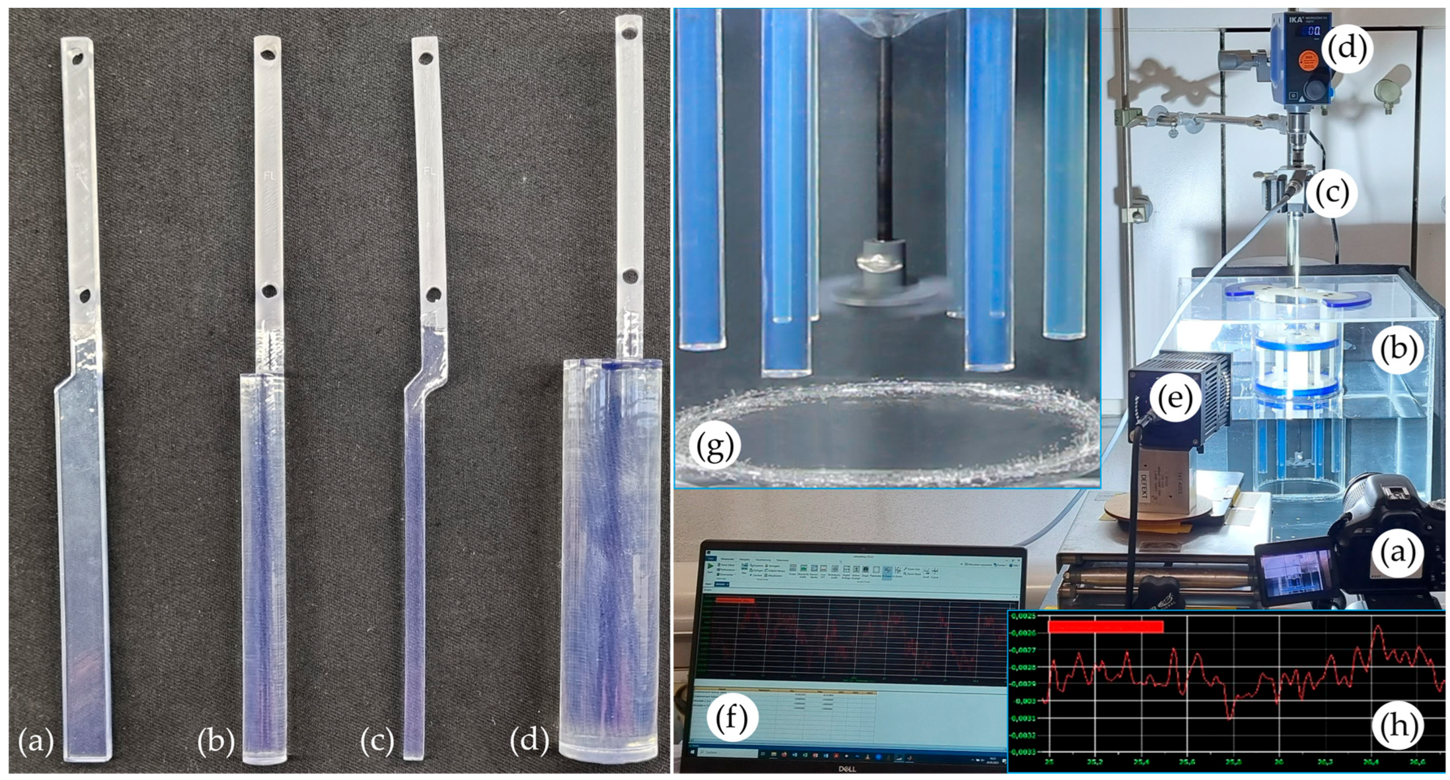
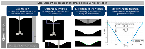
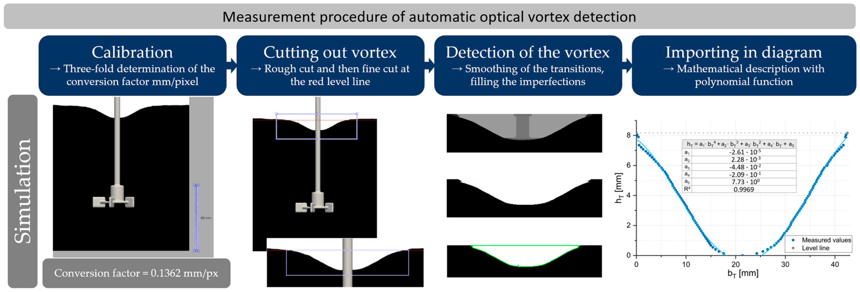
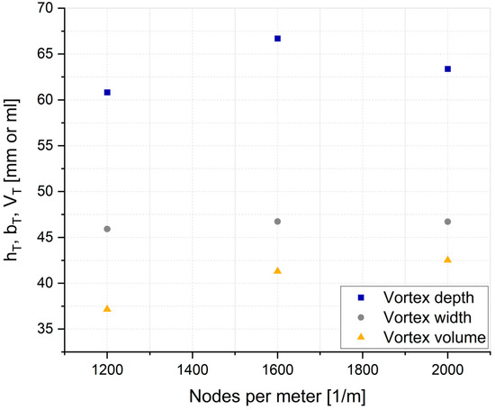
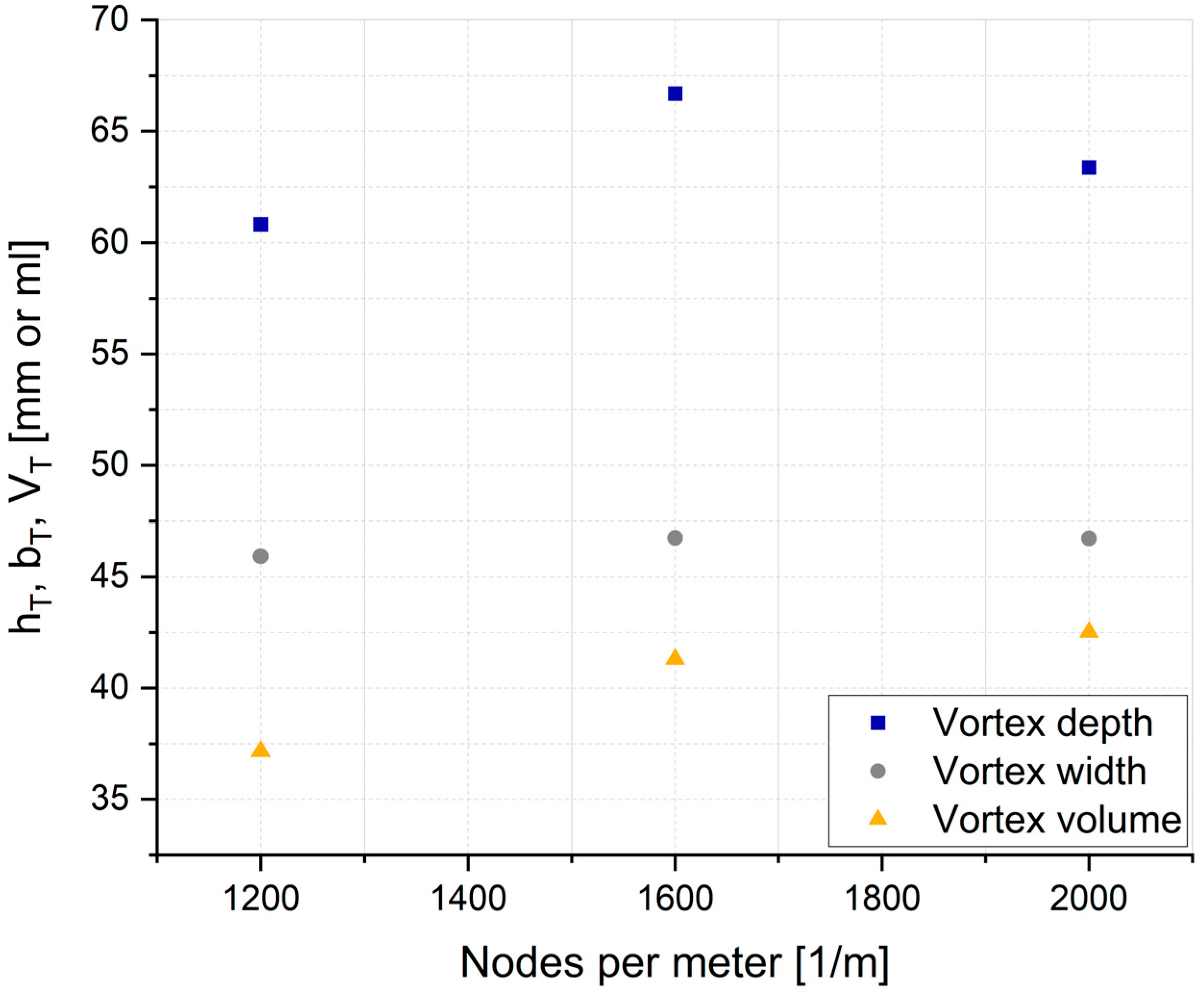
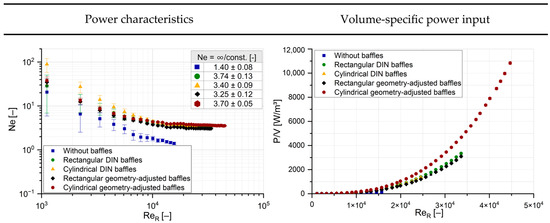
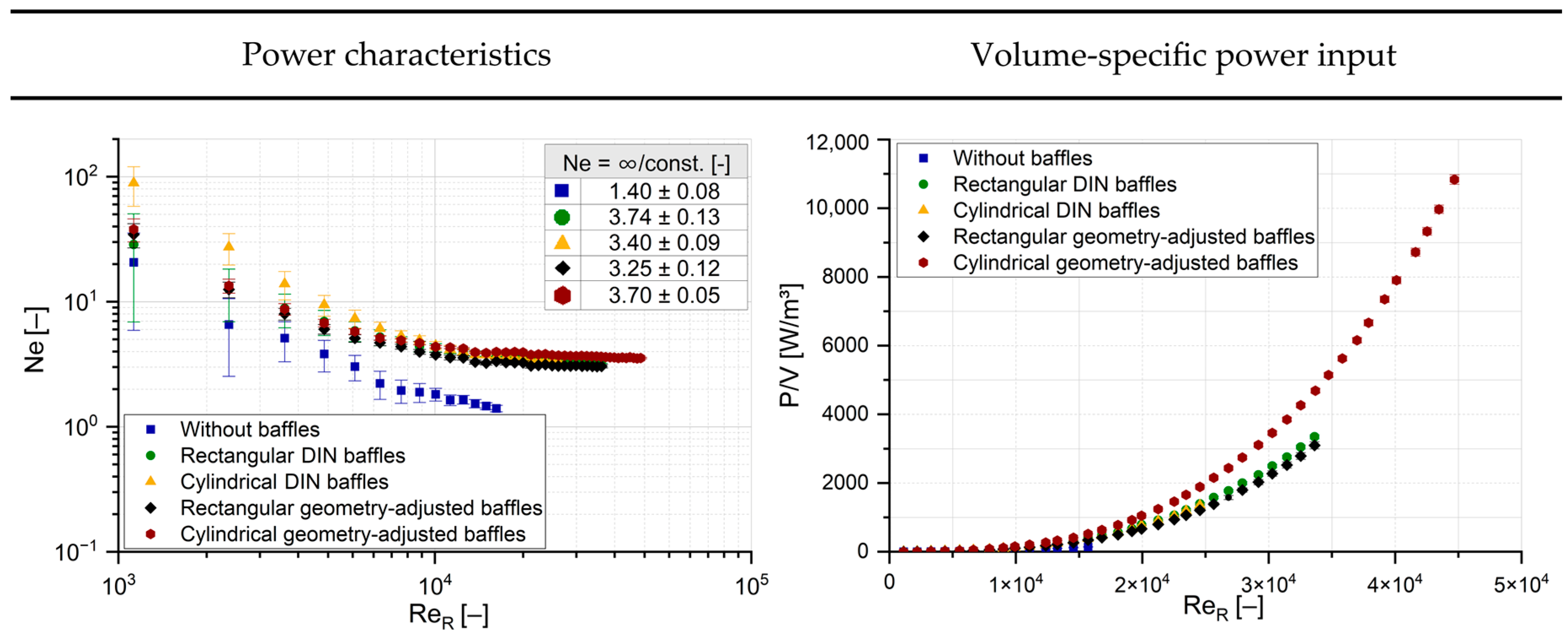
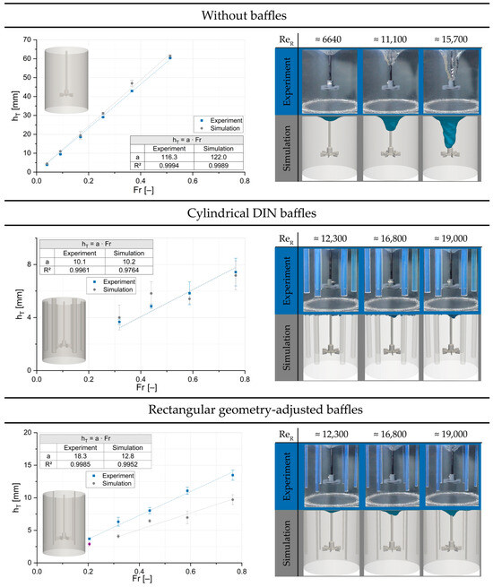
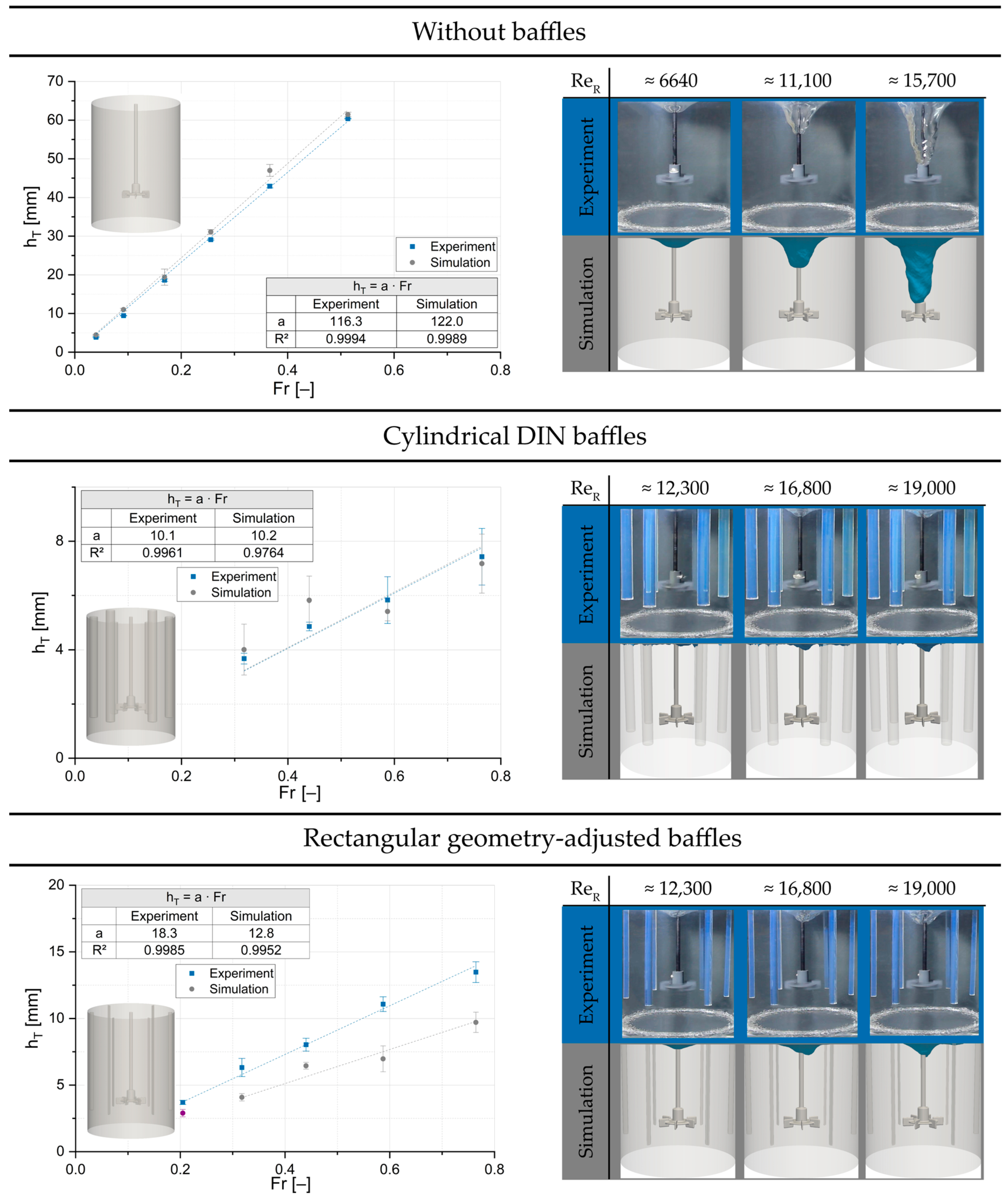
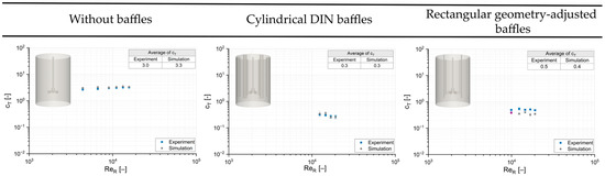
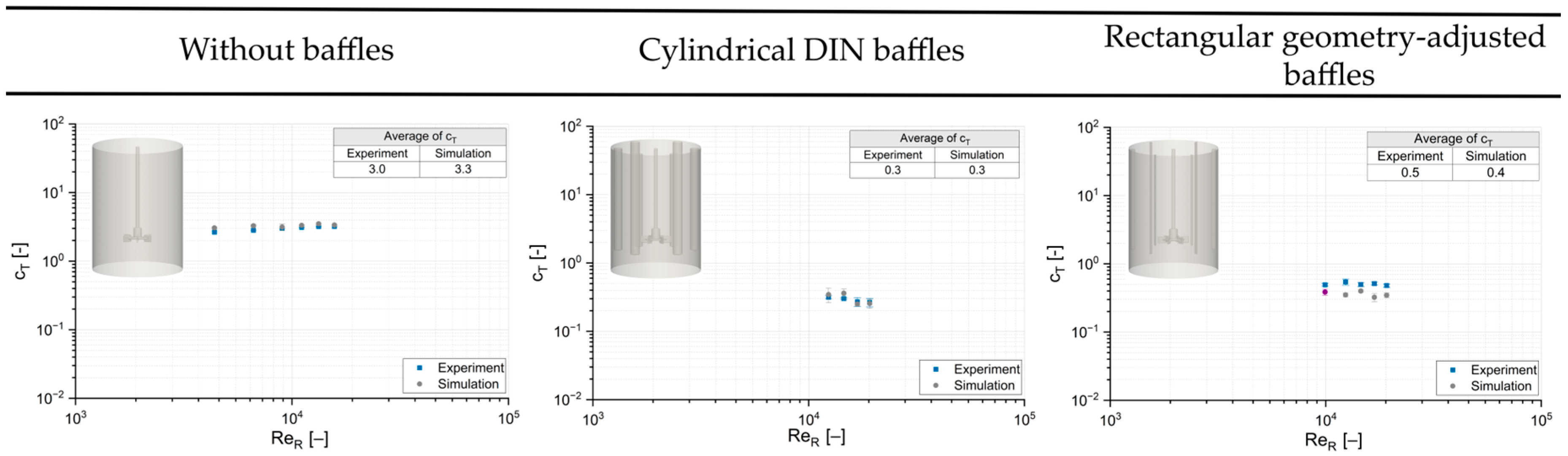
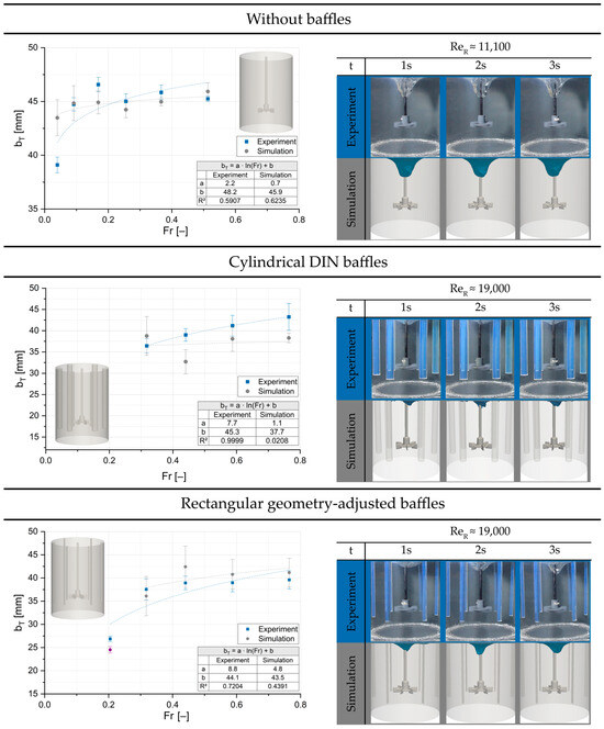
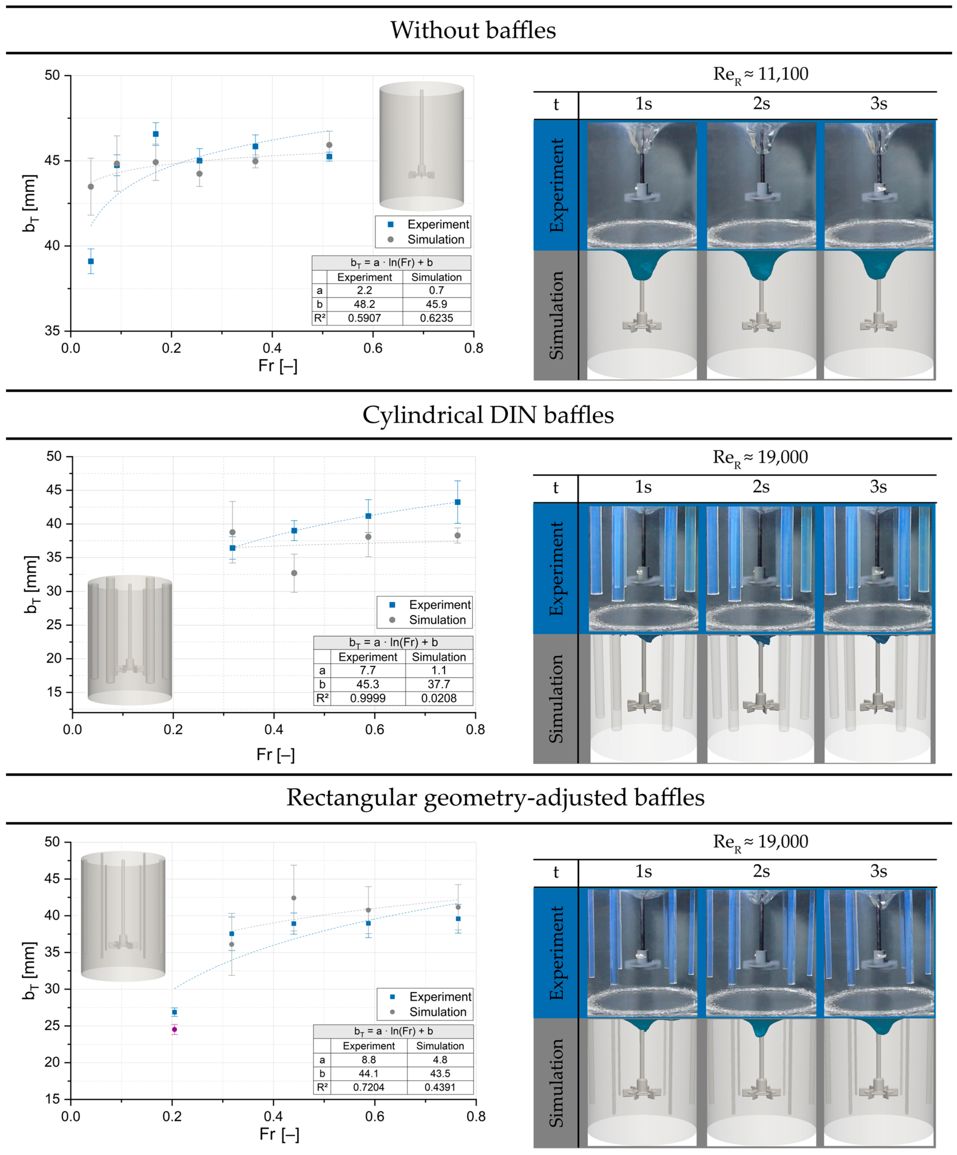
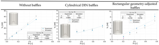
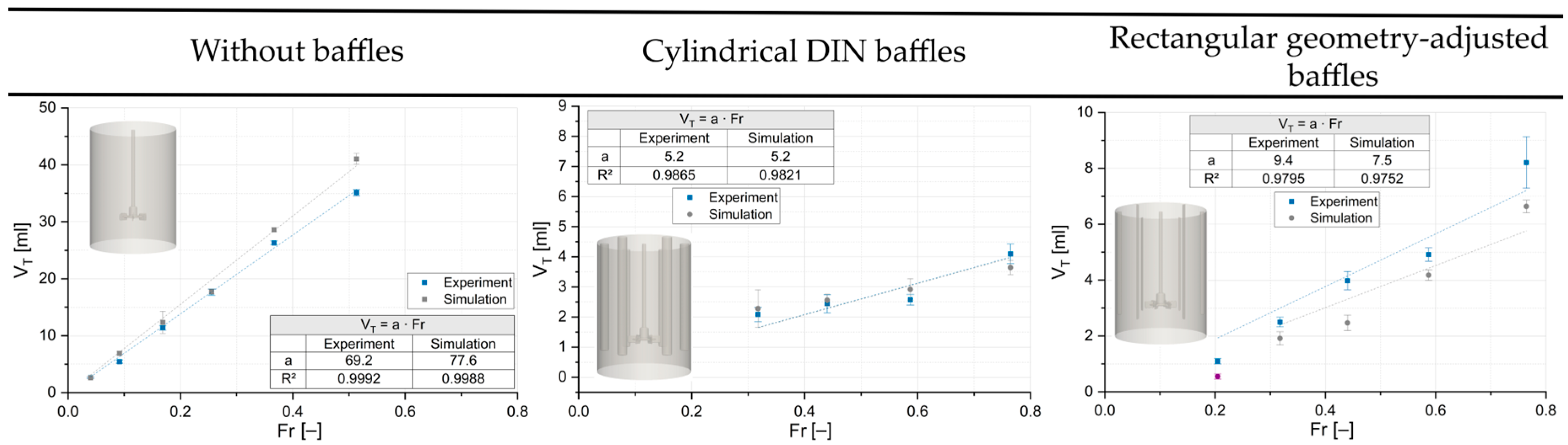
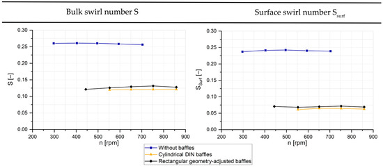
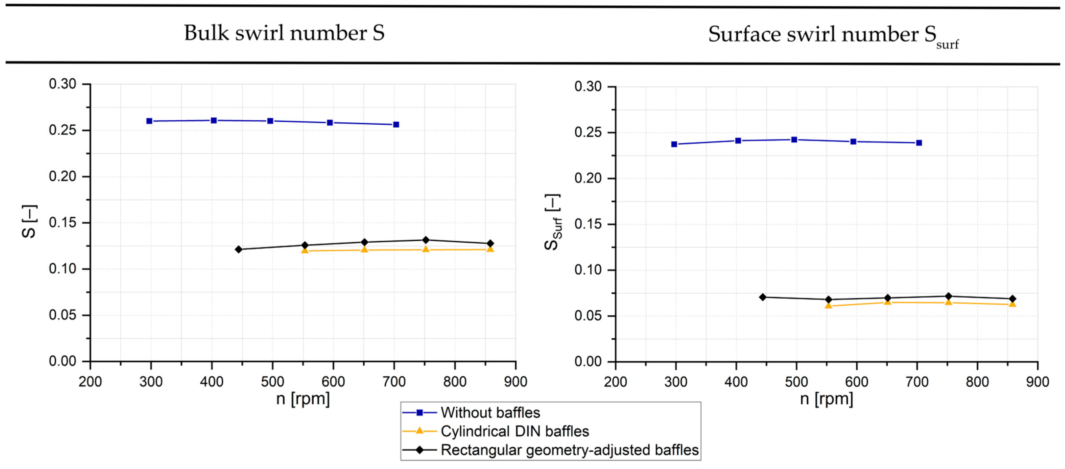
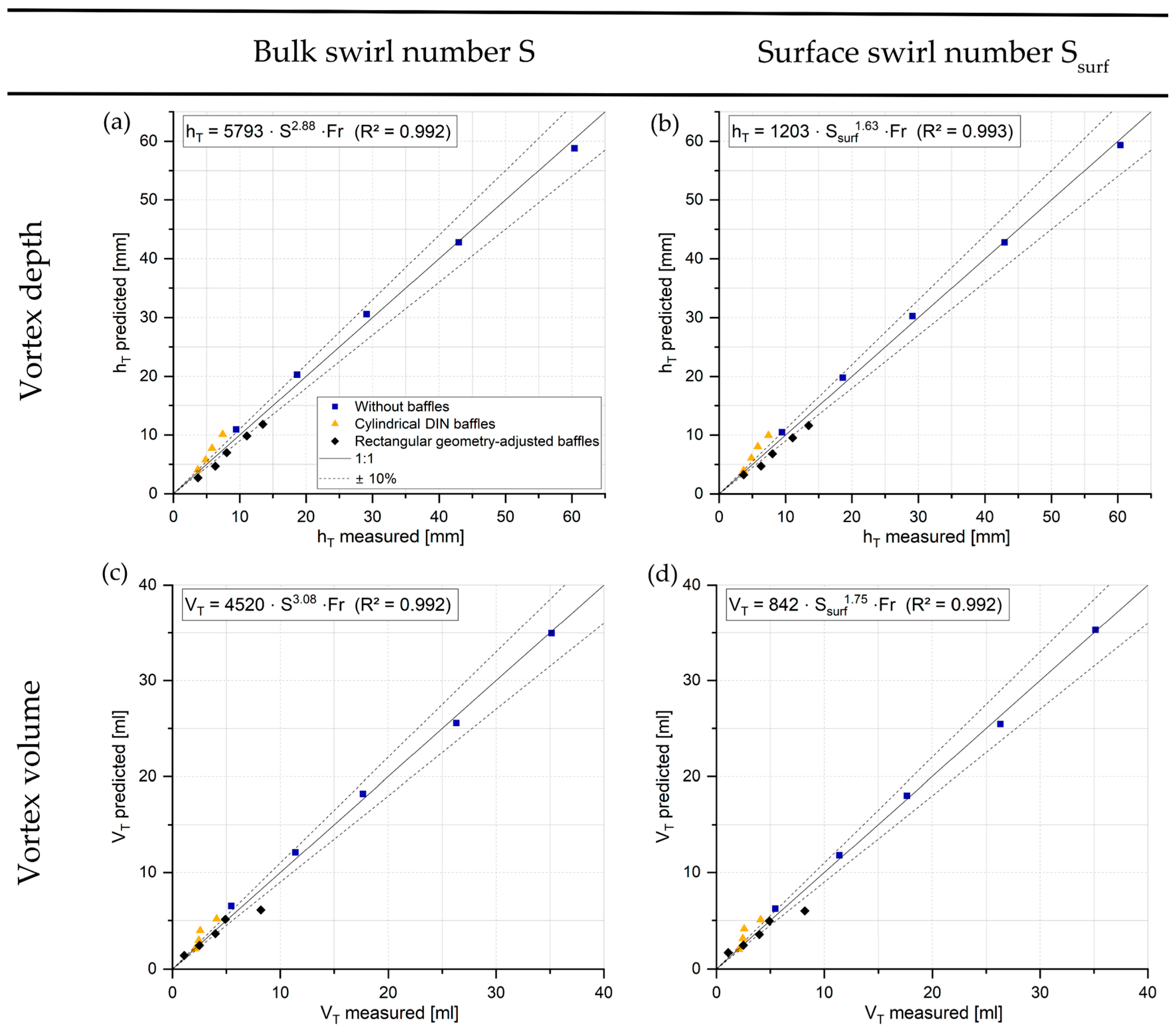
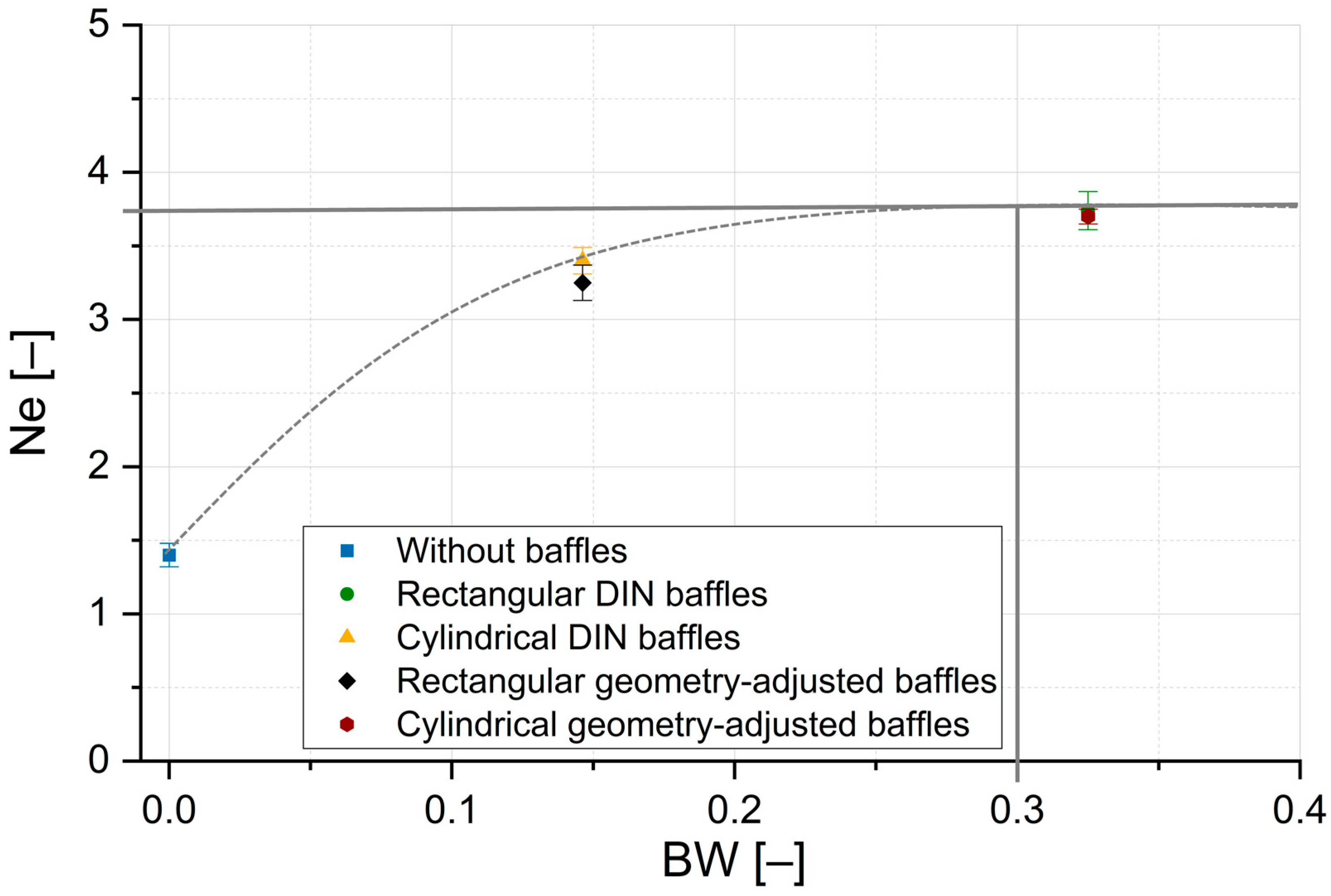

Disclaimer/Publisher’s Note: The statements, opinions and data contained in all publications are solely those of the individual author(s) and contributor(s) and not of MDPI and/or the editor(s). MDPI and/or the editor(s) disclaim responsibility for any injury to people or property resulting from any ideas, methods, instructions or products referred to in the content. |
© 2026 by the authors. Licensee MDPI, Basel, Switzerland. This article is an open access article distributed under the terms and conditions of the Creative Commons Attribution (CC BY) license.