


Abstract
Some grid-connected converters in practice are “black-box” devices with proprietary internal structures and parameters, rendering traditional model-based stability assessment infeasible. To address this issue, this paper proposes a data-driven small-signal stable operating boundary assessment method. A continuous stability evaluation index is established based on the generalized Nyquist criterion (GNC), and then the relationship between the measurable operating variables and the quantitative stability index is established by a backpropagation (BP) neural network. This mapping allows stability evaluation to rely solely on the converter’s operating states, without requiring any internal information. By implementing the stability evaluation in predefined operating scenarios, the critical stability points that reflect the small-signal stable operating boundary of the converter can be assessed. The proposed method requires only 0.0179 s to complete a single stability assessment, with an error of less than 0.25% in predicting the stable operating boundary. Simulation verifications in MATLAB/Simulink under multiple operating conditions confirm the effectiveness and accuracy of the proposed method.
1. Introduction
With the large-scale integration of renewable energy into power systems [1], converters have become important interface devices. Their widespread deployment has changed system dynamics and weakened the damping capability of power systems [2]. A mismatch between the converter impedance and the grid impedance may readily induce small-signal instability, posing a threat to the secure and stable operation of the power grid [3]. Meanwhile, the converter admittance is strongly affected by the operating point. The grid impedance also varies with the system operating mode. Both factors jointly affect the small-signal stability of a system [4]. Therefore, rapid assessment of the small-signal stability of grid-connected converter systems under dynamic operating conditions is of great importance.
Meanwhile, increasing attention has been paid to the flexibility and operational adaptability of modern power systems under changing generation and load conditions. Various methods have been proposed to assess power system flexibility [5], while flexibility enhancement, aggregation, and cooperative scheduling of distributed resources have also been investigated to improve the operational flexibility of distribution networks [6,7]. Traditional small-signal stability analysis methods can be classified into analytical model-based methods and impedance measurement-based methods. The former rely on complete system models and are further divided into eigenvalue analysis and impedance analysis. Eigenvalue analysis requires state-space models of systems [8] and evaluates system stability based on eigenvalues, damping ratios, and participation factors [9,10,11]. Impedance analysis focuses on the port frequency-domain characteristics of converters. By establishing the converter output impedance model and combining it with the grid impedance, the dynamic interactions between the converter and the grid can be analyzed [12,13]. From impedance stability theory [14] to frequency coupling effect [15,16], a comprehensive theoretical framework has been established for small-signal stability analysis using generalized impedance criteria. However, analytical model-based methods rely on detailed structural information and control parameters. For the “black-box” converter whose internal information is proprietary, this unmet prerequisite makes analytical model-based methods inapplicable. To overcome this limitation, impedance measurement-based methods have been proposed. These methods identify the converter admittance by injecting disturbance signals at the converter terminal and measuring the corresponding frequency-domain responses [17]. The identified admittance is further used to establish the overall model of the grid-connected converter system, thereby enabling stability assessment [18]. Although such methods show good adaptability to the “black-box” converter, time-varying operating conditions necessitate repeated harmonic disturbance injection for impedance measurement, which degrades power quality.
Data-driven methods that learn the mapping between operating features and stability states are regarded as a feasible approach to avoid repeated harmonic disturbance injection [19]. Existing studies have applied data-driven methods to multi-operating-point impedance model identification [20], impedance acquisition under multiple operating conditions [21], online transient stability prediction [22], and stability state identification [23], demonstrating their potential to reduce model dependence and improve assessment efficiency. A comparison of representative stability assessment methods is summarized in Table 1.
Table 1.
Comparison of different stability assessment methods.
Therefore, as summarized in Table 1, existing methods have limitations in simultaneously achieving black-box compatibility, quantitative stability margin characterization, and rapid online assessment. To address these limitations, this paper proposes a BP neural network-based rapid small-signal stability assessment method for grid-connected converter systems. This paper exploits their capabilities to learn the nonlinear mapping between operating variables and stability indices from offline samples and proposes a BP neural network-based rapid small-signal stability assessment method for grid-connected converter systems. The proposed method enables a direct mapping from measurable operating variables to a quantitative stability index under black-box conditions. The main innovations and contributions are as follows:
- (1)
- Based on analytical stability assessment, the relationship among system stability, converter admittance, and grid impedance is clarified. A quantitative assessment index is proposed to characterize the degree of system stability.
- (2)
- By incorporating physical prior knowledge, a BP neural network-based stability assessment model is constructed. Changes in converter operating points and grid impedance are considered. Taking measurable operating variables as inputs, the model enables fast mapping from the system operating state to the stability assessment index.
- (3)
- Based on the established stability assessment model, the stability boundary of the grid-connected converter system is characterized under different grid impedance conditions, providing a reference boundary for safe and stable system operation.
The rest of this paper is organized as follows. Section 2 introduces the impedance model of the grid-connected converter system and defines the quantitative stability assessment index. Section 3 constructs the BP neural network-based stability assessment model. The online stability assessment process and the stable operating boundary characterization method are also presented. The accuracy and effectiveness of the proposed method are verified through simulation results under different operating conditions in Section 4. Section 5 concludes this paper.
2. Impedance Modeling and Stability Assessment
In this section, an impedance model of the grid-following converter is established. Based on the generalized Nyquist stability criterion (GNC), a stability assessment index capable of quantitatively evaluating the system stability margin is proposed. Furthermore, the effects of operating point and grid impedance variations on the system stability margin are analyzed.
2.1. Impedance Model of the Grid-Connected Converter System
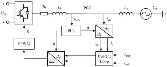
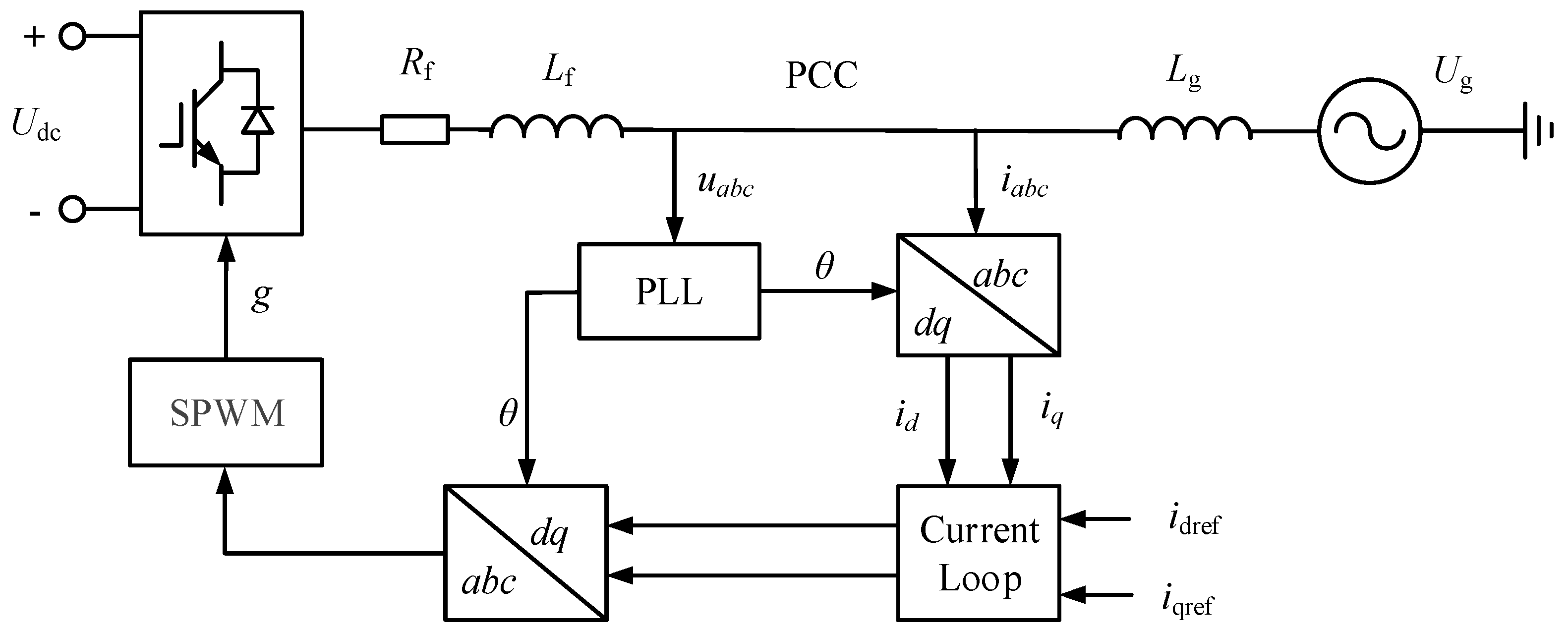
Figure 1 illustrates the main circuit topology and the control block diagram of the grid-connected converter system. The converter is connected to the point of common coupling (PCC) through an L-type filter, while the grid current is regulated by a phase-locked loop (PLL) and an inner current control loop. Here, Udc denotes the DC-link voltage source, Lf is the filter inductance, Rf is the equivalent parasitic resistance of the filter inductance, Lg represents the equivalent grid inductance, and Ug denotes the ideal grid voltage source.
Figure 1.
Structure of the grid-connected converter system.
Based on the main circuit and control system shown in Figure 1, the impedance model of the converter can be derived using the small-signal linearization method [24] as:
where Gplli and Gplld represent the transfer functions from the voltage perturbation to the current and duty-cycle command, respectively; Gci is the transfer function of the PI current controller; Gdei denotes the decoupling term of the current control loop; Gdel is the equivalent delay transfer function; Zout is the open-loop output impedance; Gid is the transfer function from the duty-cycle command to the converter bridge arm output voltage; and E is the identity matrix.
The grid impedance can be expressed as
where s is the Laplace operator and ω0 denotes the fundamental angular frequency.
2.2. Stability Assessment of the Grid-Connected System
Based on the established impedance model of the grid-following converter, the GNC [25] is employed to derive a quantitative stability assessment index. Furthermore, the effects of variations in the converter operating point and grid impedance on the system stability are analyzed, thereby revealing the intrinsic relationship between operating conditions and the system stability margin.
According to the GNC, the stability of the grid-connected converter system can be determined by whether the eigenvalue trajectories of the return-ratio matrix encircle the critical point (−1, j0). The return-ratio matrix is expressed as:
A stability assessment index is extracted from the intersections between the eigenvalue trajectories of the return-ratio matrix and the negative real axis. Specifically, the magnitude of each eigenvalue at the frequency where its phase equals −180° is selected as the stability assessment index. Since the overall system stability is dominated by the oscillation mode closest to the stability boundary, the smaller of the two stability margins is adopted as the final stability assessment index S, which is defined as:
where λ() denotes the complex eigenvalue of the impedance ratio matrix; ωc1 and ωc2 are the critical angular frequencies at which the phases of the two eigenvalues reach −180°, respectively; S1 and S2 denote the corresponding stability margins of the two oscillation modes; and S represents the overall stability assessment index of the system. The proposed index S provides a continuous measure of the system stability margin. When S < 0, the system is stable, and a larger absolute value of S indicates a greater stability margin. When S = 0, the system is at the critical stability boundary. When S > 0, the system becomes unstable, and a larger value of S indicates a more severe degree of instability.
The stability assessment index S is determined by the impedance ratio matrix formed by the grid impedance Zg and the converter output impedance Zinv. Therefore, it depends on both the grid and converter impedance characteristics. According to (5), the converter impedance varies with the operating point, i.e.,
where U is the PCC voltage and Id, Iq are the d-axis and q-axis components of the PCC current, respectively.
Therefore, the stability assessment index S is jointly determined by the converter operating point and the grid impedance. To verify their effects on system stability, these two factors are varied independently. For a given grid impedance, the voltage and current at the point of common coupling satisfy the port impedance relationship. Therefore, under the condition of unity power factor, the variation in operating points can be characterized by adjusting Id.
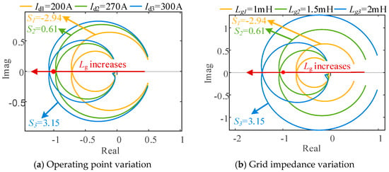
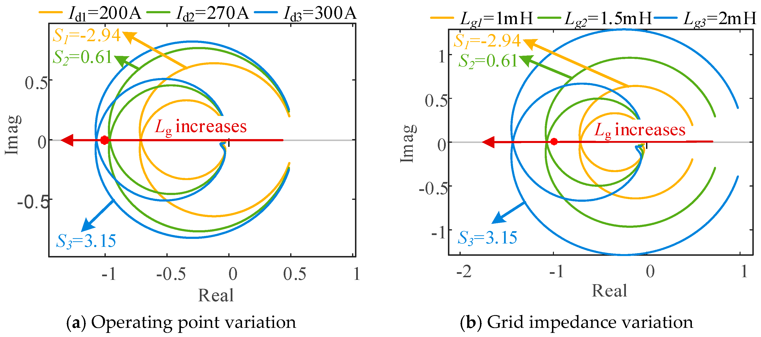
Figure 2 presents the Nyquist trajectories of the system eigenvalues under different operating conditions. As shown in Figure 2a, the Nyquist trajectories gradually approach the critical point (−1, j0) as Id increases, resulting in a reduced stability margin. When Id reaches 300 A, the trajectory encircles the critical point, and the system becomes unstable. Figure 2b shows the effect of grid impedance with a constant Id. When Lg = 1 mH, the Nyquist trajectory remains inside the unit circle and maintains a sufficient distance from the critical point. As Lg increases to 1.5 mH, the trajectory encircles the critical point, resulting in system instability.
Figure 2.
Nyquist trajectories of system eigenvalues under different operating conditions.
The above results indicate that the system stability is jointly determined by the operating point and the grid impedance. These factors determine the Nyquist trajectories and their proximity to the critical point. Increasing either the grid-connected current or the grid impedance reduces the stability margin, eventually leading to oscillatory instability.
3. Data-Driven Small-Signal Stability Assessment
This section develops a data-driven stability assessment model based on the stability assessment index established in the previous section. By learning the nonlinear mapping between the operating conditions and the stability assessment index, the proposed model enables rapid stability assessment and fast characterization of the stable operating boundary under dynamic operating conditions.
3.1. Analysis of the Input and Output Variables for Stability Assessment
As discussed in the previous section, the stability assessment index S of the grid-connected converter system is a nonlinear function of the converter operating conditions and the grid impedance, which can be expressed as:
where f denotes the nonlinear mapping determined by the system dynamics.
Accordingly, the inputs of the stability assessment model are the grid inductance Lg, PCC voltage U, and PCC current components Id and Iq, while the output is the stability assessment index S, defined as the eigenvalue magnitude at the critical phase.
3.2. BP Neural Network-Based Stability Assessment Method
The objective of the stability assessment model is to establish the nonlinear mapping between the operating conditions and the system stability margin, which is essentially a regression problem. Owing to its strong nonlinear approximation capability, clear network architecture, and mature training algorithms, the BP neural network is adopted to construct the stability assessment model for the grid-connected converter system. The model development consists of three stages: data acquisition, data preprocessing, model construction and training.
3.2.1. Data Acquisition
In practical applications, converter manufacturers usually provide black-box simulation models of their products. Therefore, the port impedance of the converter under different operating points can be obtained using the frequency sweep method without requiring knowledge of the internal control structure or parameters. The measured converter impedance is then combined with the grid impedance to construct the impedance ratio matrix L(s), from which the stability assessment index is calculated according to (4).
3.2.2. Data Preprocessing
As described in Section 2, the proposed neural network model has four input variables, namely, the converter operating conditions and the grid impedance. The output variable is the system stability assessment index. Since the input features and output labels differ significantly in magnitude and physical units, directly using the raw data for training will slow the convergence process and degrade prediction accuracy. Therefore, both the input features and output labels are normalized before training. The normalization is given by:
where x denotes the original variable; xmax and xmin are the maximum and minimum values of the corresponding variable, respectively; and xnom is the normalized value.
3.2.3. Model Construction and Training
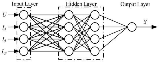
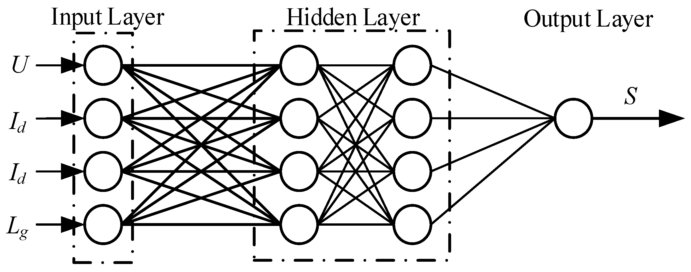
The architecture of the BP neural network is shown in Figure 3. The input layer consists of four neurons corresponding to the converter operating conditions and the grid impedance. The hidden layer, composed of multiple neurons with nonlinear activation functions, is employed to capture the nonlinear relationship between the operating conditions and the system stability margin. The output layer contains one neuron representing the stability assessment index. During training, the network parameters are iteratively optimized by minimizing the loss function, enabling the model to progressively learn the nonlinear mapping between the operating conditions and the stability assessment index.
Figure 3.
Architecture of the BP neural network.
To determine an appropriate hidden-layer architecture, a comparative study was conducted using five different network configurations, including 1 × 5, 1 × 10, 2 × 5, 2 × 10, and 3 × 5, where the first and second numbers denote the number of hidden layers and the number of neurons in each hidden layer, respectively. All configurations were trained using the same dataset, data preprocessing procedure, and Bayesian regularization algorithm. The training RMSE, testing RMSE, and training time were used to evaluate the prediction accuracy and computational efficiency of different network architectures, as summarized in Table 2.
Table 2.
Comparison of BP neural networks with different hidden-layer configurations.
As shown in Table 2, increasing the network complexity from 1 × 5 to 2 × 5 improves the prediction accuracy, with the 2 × 5 configuration achieving the lowest testing RMSE of 0.019897. Further increasing the network complexity to 2 × 10 and 3 × 5 does not improve the testing performance. Therefore, considering prediction accuracy, network complexity, and training efficiency, the 2 × 5 configuration is selected for the proposed stability assessment model.
To improve the generalization capability of the model, the BP neural network is trained using the Bayesian regularization algorithm. During training, the network weights and biases are not manually selected but are automatically initialized and iteratively updated through the backpropagation algorithm by minimizing the training objective function. In this study, Bayesian regularization is incorporated into the training process, where both the prediction error and the weight penalty are considered to determine the optimal network parameters. Compared with the conventional BP algorithm, Bayesian regularization introduces a weight penalty term into the loss function and automatically updates the regularization parameters α and β during training. As a result, the model can balance fitting accuracy and complexity. The objective function is defined as
where ED denotes the prediction error between the network output and the target value, which is typically evaluated by the mean squared error. Ew is the sum of squared network weights, representing the model complexity. α and β are the regularization parameters that determine the relative weights of the error term and the weight penalty term, respectively.
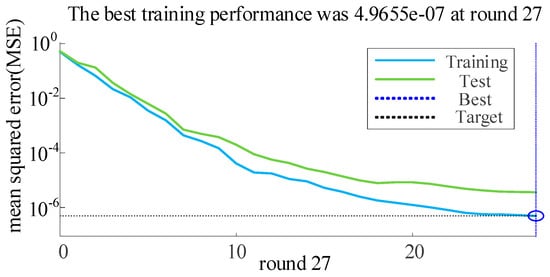
To further evaluate the convergence performance of the BP neural network, the mean squared error (MSE) during the training and testing processes is analyzed, as shown in Figure 4. The best training performance is achieved at the 27th training iteration, where the MSE reaches 4.9655 × 10⁻⁷. The network reaches a very low prediction error within a limited number of training iterations, indicating a relatively rapid convergence for the considered grid-connected converter stability assessment problem. In addition, the training and testing performance curves exhibit consistent convergence trends, demonstrating the effectiveness of the adopted Bayesian regularization strategy in obtaining a stable and generalized neural network model. To further verify the effectiveness of Bayesian regularization, the training performance of the proposed BP neural network is compared with that of a conventional BP neural network without Bayesian regularization, as shown in Figure 5.
Figure 4.
Training performance of the BP neural network with Bayesian regularization.
Figure 5.
Training performance of a conventional BP neural network.
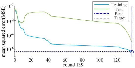
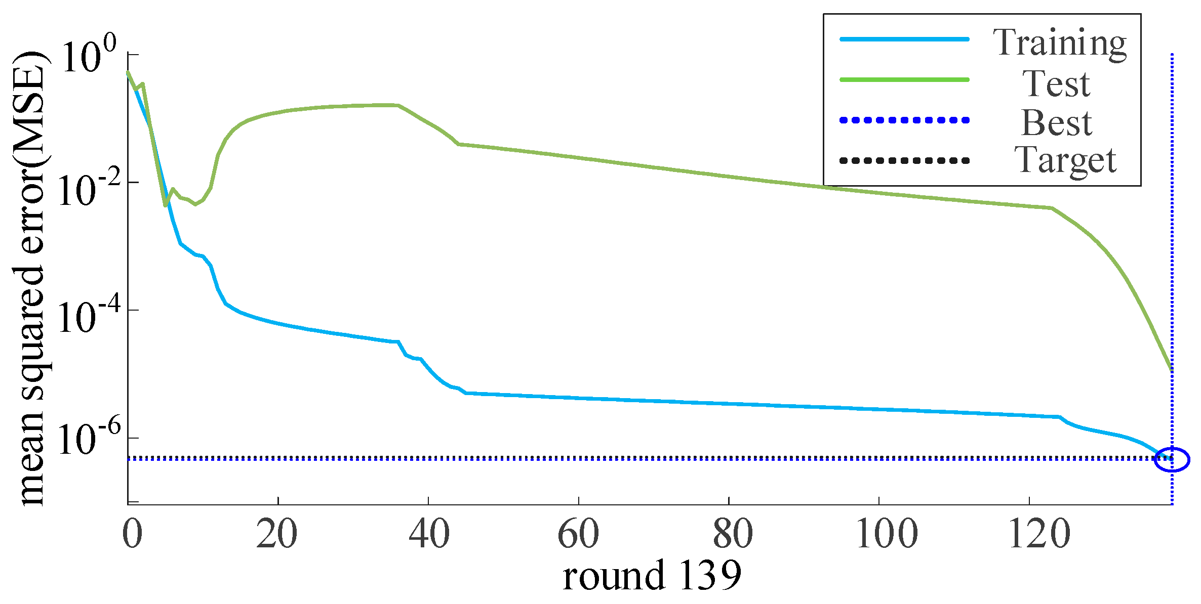
In contrast, as shown in Figure 5, the conventional BP neural network requires 139 epochs to reach its best performance, and a pronounced gap between the training and test errors can be observed, indicating a stronger overfitting tendency. Therefore, the introduction of Bayesian regularization improves the generalization capability of the BP neural network and enables more stable convergence with fewer training epochs. Based on these results, the BP neural network with Bayesian regularization is selected as the training method for the proposed data-driven stability assessment model, owing to its better generalization capability and reduced overfitting tendency.
3.3. Online Stability Assessment and Stable Operating Boundary Characterization
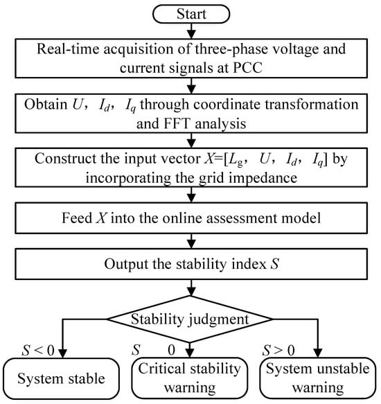
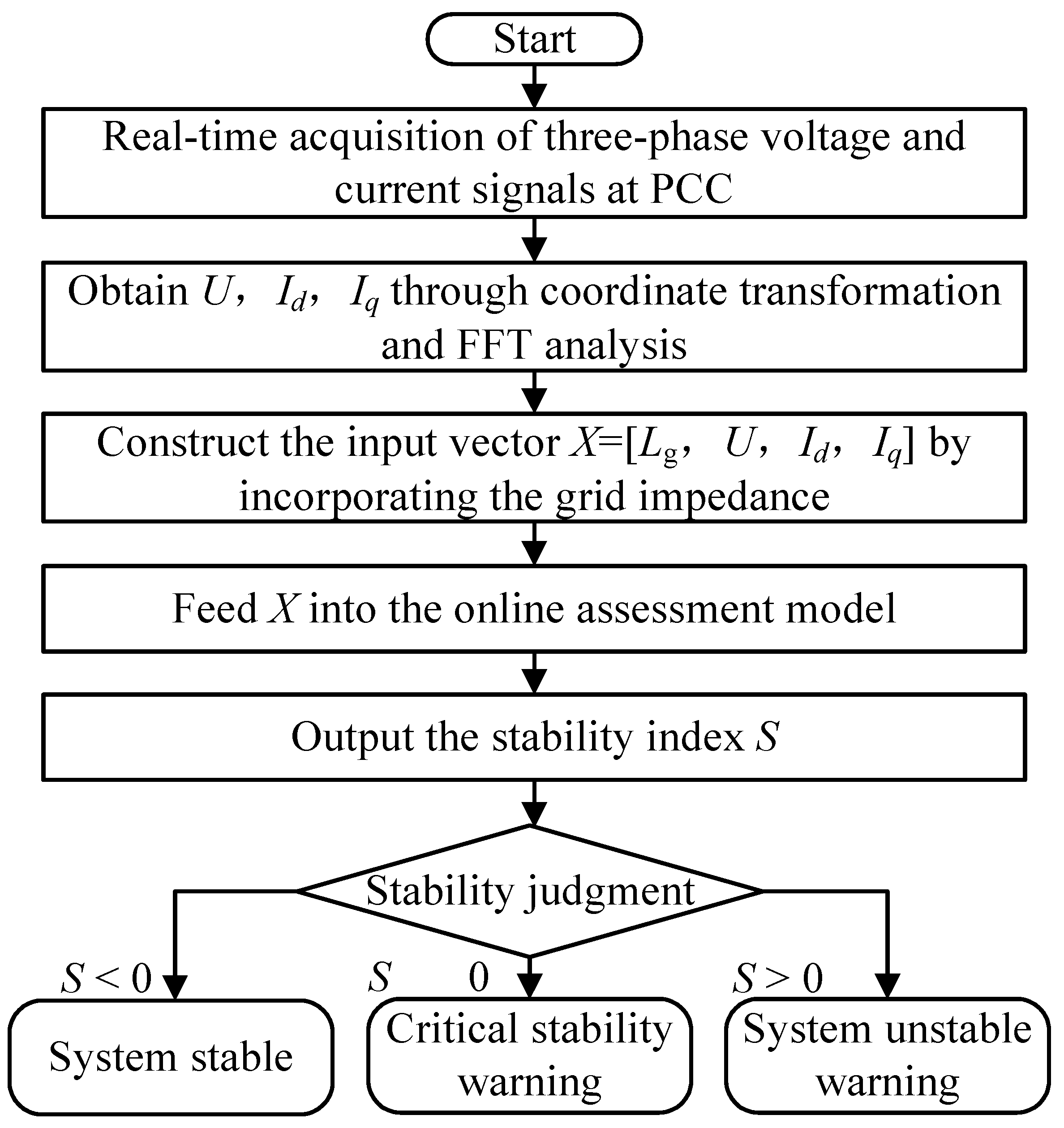
Based on the established BP neural network-based stability assessment model, online stability assessment is further conducted. In the proposed framework, the term “black-box converter” refers to the unavailability of the converter’s internal control structure, parameters, and impedance model. The grid-side equivalent impedance is not treated as a black-box quantity. Instead, the grid inductance Lg is regarded as an externally available grid parameter. In practical applications, the voltage and current measurements at the PCC can be obtained using the existing electrical measurement system, and Lg can be estimated online using established grid impedance estimation techniques. Passive estimation methods based on naturally available voltage and current information can obtain the grid impedance without intentionally injecting additional disturbance signals [26,27]. Therefore, the proposed method does not require repeated online impedance measurements of the black-box converter; the estimated Lg, together with the measured PCC voltage and current, is used as the input of the trained neural network. In the online stage, measurable operating information, including the point of common coupling voltage, current, and grid impedance, is collected in real time to construct the input vector. The input vector is then fed into the trained model to predict the stability assessment index S, thereby enabling rapid evaluation of the system stability and stability margin. The overall online assessment procedure is illustrated in Figure 6. The obtained results can be further utilized for instability warning and subsequent control decision-making.
Figure 6.
Flowchart of the online stability assessment.
Furthermore, the parameters Lg, U, Id, and Iq are sampled over predefined ranges to generate multiple operating conditions. These operating conditions are then evaluated using the trained stability assessment model. By extracting the set of operating points corresponding to the stability boundary from the prediction results, the stable operating boundary can be constructed. This boundary characterizes the stable operating region under different converter operating points and grid impedances, providing stability constraints for system operation and controller design.
4. Case Studies
4.1. System Description
The three-phase L-type grid-connected converter system shown in Figure 1 is taken as an example to verify the correctness and effectiveness of the proposed data-driven online stability assessment method for the grid-connected converter system. The main parameters of the grid-connected converter system are listed in Appendix A, Table A1. The converter is connected to the grid through the filter and grid-side inductance Lg, and the PCC voltage and current are selected as the key operating variables. The selected parameter ranges are intended to cover different grid strength conditions and converter operating states, thereby providing a representative test environment for evaluating the proposed online stability assessment method. The benchmark operating conditions are selected with reference to applicable interconnection requirements for inverter-based resources, while the small-signal stability assessment is performed according to the stability criterion adopted in this study. The nominal operating conditions are shown in Table 3.
Table 3.
Nominal benchmark parameters.
Under this benchmark condition, the stability index calculated from the original system model is −2.940513, while the value predicted by the proposed BP neural network with Bayesian regularization is −2.940859. The corresponding absolute error is only 0.000346, with a relative error of approximately 0.0118%. The close agreement between the reference and predicted values verifies the accuracy of the proposed stability assessment method under the benchmark operating condition.
4.2. Data-Driven Stability Assessment of the Grid-Connected Converter System
(1) Data Acquisition. A time-domain simulation model of the grid-connected converter system is established in MATLAB/Simulink. The frequency sweep method is employed to obtain the dq impedance matrix of the converter under different operating points. The measured converter impedance is then combined with the corresponding grid impedance to construct the impedance ratio matrix. The stability assessment index S under each operating condition is calculated as the eigenvalue magnitude at the frequency where the eigenvalue phase reaches −180°. The equivalent grid inductance is varied from 1 mH to 2 mH with an interval of 0.2 mH, resulting in six grid conditions. Accordingly, a sample dataset containing the operating conditions, grid impedance, and stability assessment index is established, which can be expressed as ({(U, Id, Iq, Lg) → S}). A total of 600 samples are obtained.
(2) Data Preprocessing. Both the input variables and the output labels are normalized to the range of [−1, 1] according to (7). The dataset is then divided into training, validation, and test sets with a ratio of 70%:15%:15%. It should be noted that during online assessment, newly collected data should be processed using the same normalization parameters as those used in the training stage, and model outputs should be denormalized to ensure consistency in data scaling between the training and application stages.
(3) Construction and Training of the Neural Network Model. The input layer of the BP neural network contains four neurons, corresponding to (Lg, U, Id, Iq). The hidden layer consists of two layers, each containing five neurons. The output layer contains one neuron, corresponding to the stability assessment index S. Bayesian regularization is adopted to train the network. The regularization parameters are automatically adjusted during the training process, thereby producing smoother and more stable model outputs.
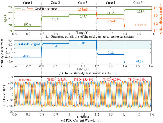
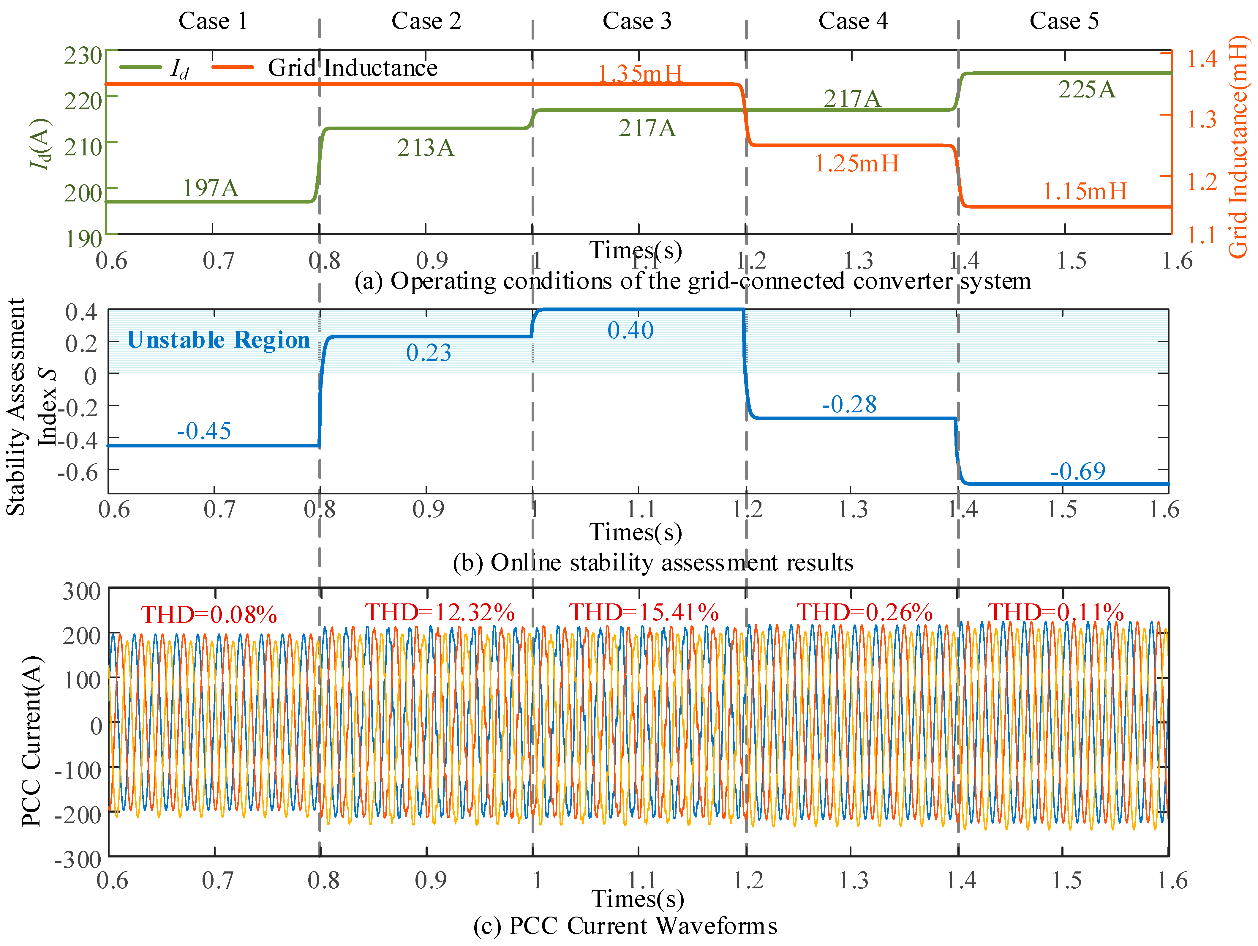
(4) Online Stability Assessment of the Grid-Connected Converter System. The simulation model of the grid-connected converter system shown in Figure 1 is established in the MATLAB/Simulink platform. Operating conditions with different current operating points Id and grid inductance Lg are set to verify the accuracy of the established BP neural network-based stability assessment model. Figure 7 presents the online stability assessment results under different operating conditions, together with the corresponding time-domain simulation results. The detailed analysis of each operating condition is presented as follows.
Figure 7.
Online stability assessment results based on the BP neural network.
① Case 1: Initially, the reference value of Id is set to 197 A, and the grid inductance is 1.35 mH. The online stability assessment is performed using the proposed stability assessment model. The predicted stability assessment index S is −0.45, indicating that the system is stable. The time-domain simulation results also show that the PCC current remains stable, and the total harmonic distortion (THD) is only 0.08%. This result is consistent with the online stability assessment.
② Case 2: At 0.8 s, the reference value of Id is increased to 213 A, while the grid inductance remains unchanged. The predicted value of S becomes 0.23, indicating that the system crosses the stability boundary and enters the unstable region. Correspondingly, obvious oscillations are observed in the PCC current waveforms. The THD increases to 12.32%, indicating that the system becomes oscillatory.
③ Case 3: At 1.0 s, the reference value of Id is further increased to 217 A, while the grid inductance still remains unchanged. The predicted value of S increases to 0.40, indicating that the stability margin is further reduced. Correspondingly, more severe oscillations are observed in the three-phase current. The THD further increases to 15.41%.
④ Case 4: At 1.2 s, the reference value of Id remains unchanged, while the grid inductance is reduced to 1.25 mH. The predicted value of S changes to −0.28, indicating that the system returns to the stable region. Correspondingly, the PCC current is restored to a stable state, and the THD decreases to 0.26%.
⑤ Case 5: At 1.4 s, the reference value of Id is increased to 225 A, while the grid inductance is reduced to 1.15 mH. The predicted value of S changes to −0.69, indicating that the system returns to the stable region. Correspondingly, the PCC current is restored to a stable state, and the THD decreases to 0.11%.
The online assessment speed based on a neural network model is mainly determined by the computational capability of the computer used for analysis. The personal computer used in this paper is configured as follows: (1) CPU: Intel(R) Core(TM) i5-14600KF @ 3.50 GHz; (2) RAM: 32 GB; (3) GPU: NVIDIA GeForce RTX 3050; and (4) software platform: MATLAB R2022a. Under this hardware and software environment, the computation time required for a single stability assessment, from the input of Lg, U, Id, and Iq to the output of the stability assessment index, is 0.0179 s. For comparison, the conventional impedance-based stability assessment requires two main steps. First, the converter impedance matrix is obtained through frequency scanning, which requires approximately 5 min under the same simulation environment. Second, the obtained impedance matrix is combined with the grid impedance and analyzed using the generalized Nyquist criterion to obtain the stability assessment index. Therefore, the conventional method requires a substantially longer computational time than the proposed neural network-based method. Therefore, the proposed method satisfies the requirement for online stability assessment of the grid-connected converter system.
The above simulation results show that the proposed stability assessment model can output the stability assessment index S in real time according to variations in the operating point and grid impedance during system operation. The obtained index accurately reflects the dynamic evolution of the system stability state.
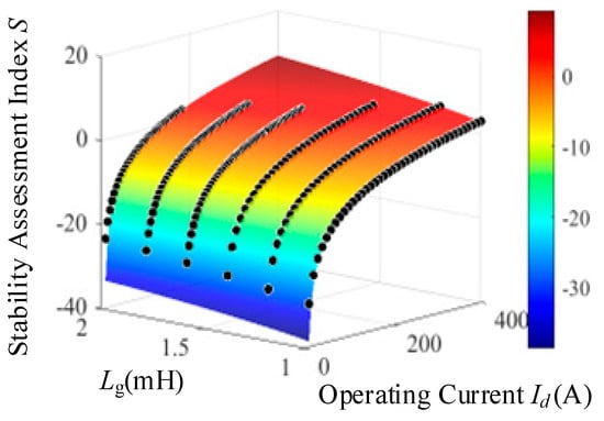
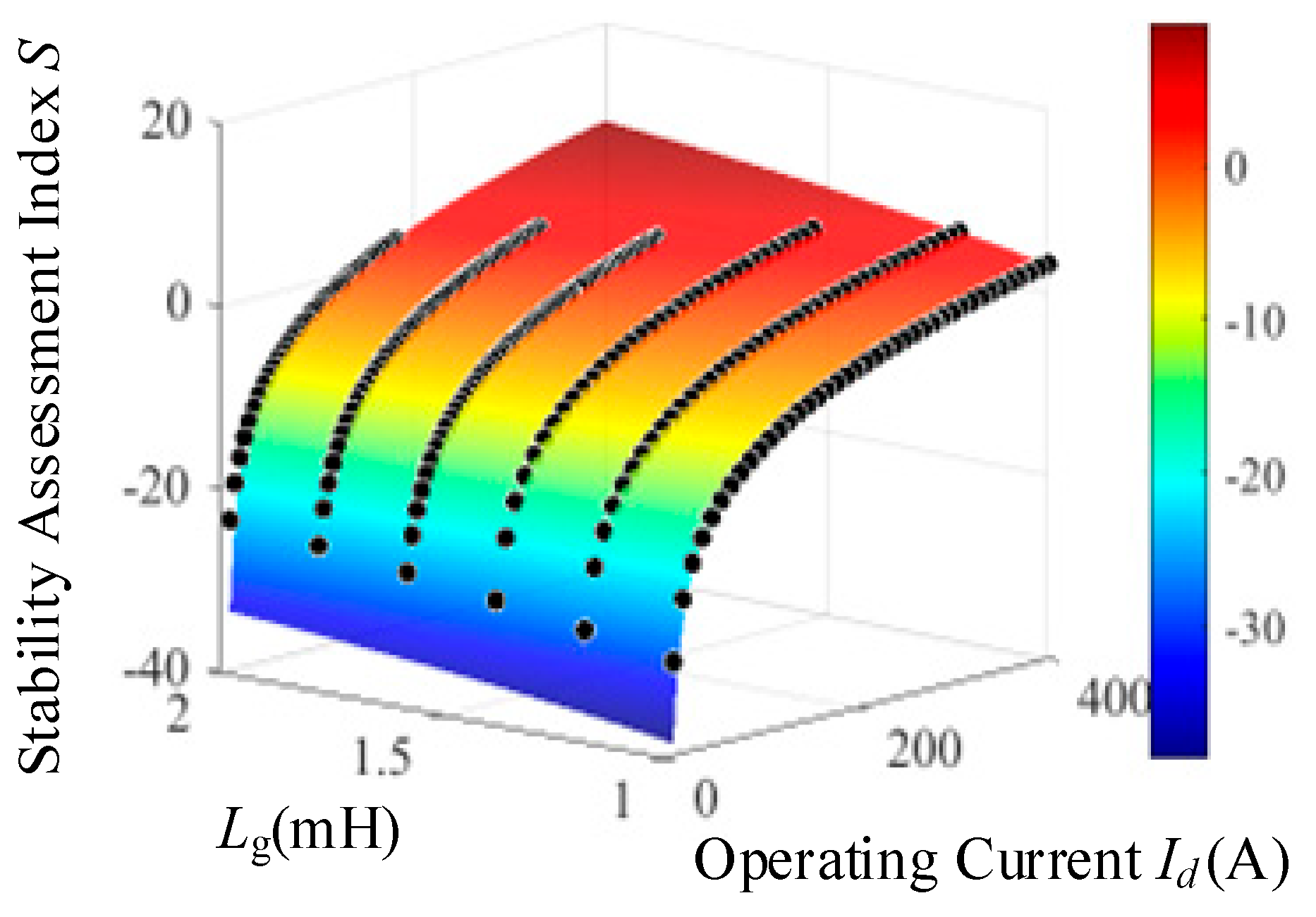
(5) Verification of the Stable Operating Boundary. Based on the trained stability assessment model, the critical operating points are extracted from the prediction results over the entire operating range. The stable operating boundary of the grid-connected converter system under different grid impedances and current Id values is then characterized, as shown in Figure 8. In Figure 8, the colored surface represents the stability prediction surface obtained by the neural network, while the black dots represent the sample data. It can be observed that good agreement is achieved between the sample data and the predicted stable operating boundary. This indicates that the trained stability assessment model can accurately capture the nonlinear relationship among the grid impedance, the operating current, and the stability assessment index S. Although the training data are obtained from a limited number of operating points, a continuous prediction surface is constructed by the stability assessment model. As a result, the stability assessment index at unmeasured operating points can be effectively estimated.
Figure 8.
Stable operating boundary.
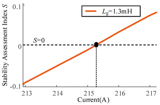
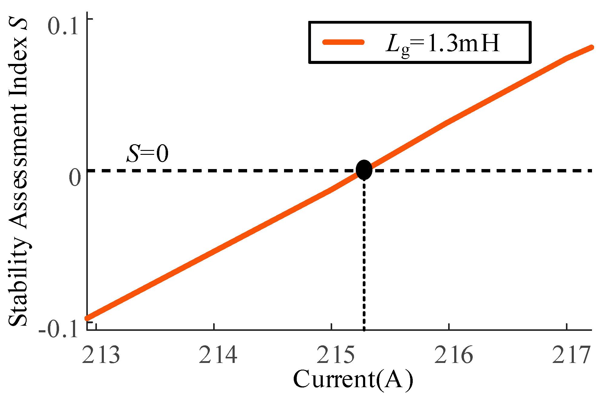
To verify the accuracy of the predicted stable operating boundary, a case with Lg = 1.3 mH is considered. As shown in Figure 9, the predicted critical current corresponding to S = 0 is 215 A.
Figure 9.
Stable operating boundaries under Lg = 1.3 mH.
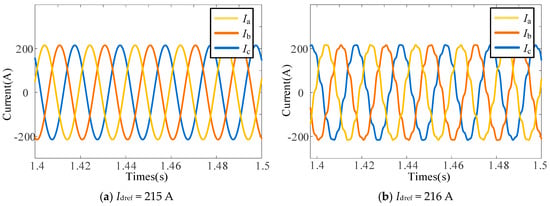
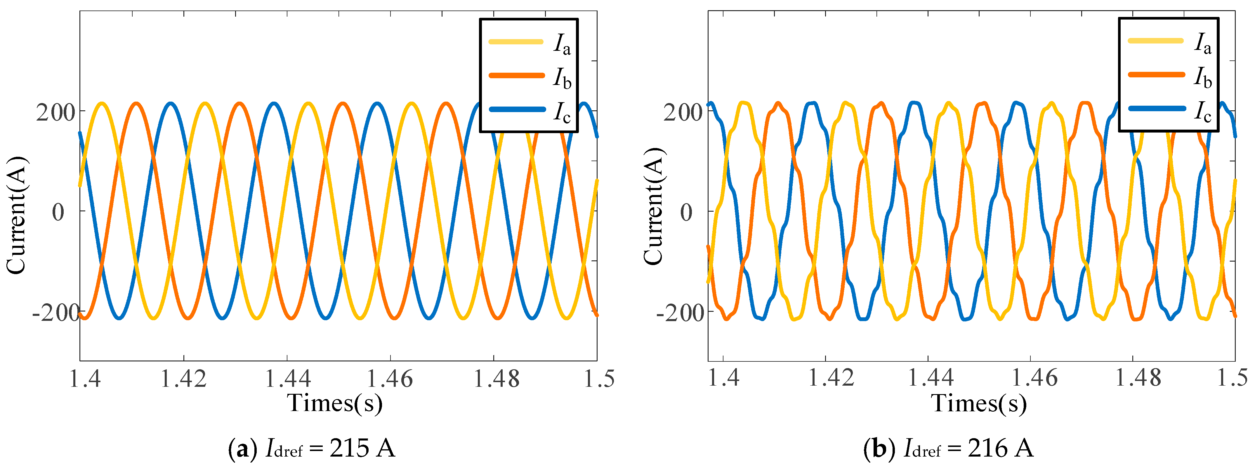
As shown in Figure 10, the PCC current remains stable when Id = 215 A, while obvious oscillations occur when Id increases to 216 A. This result is consistent with the predicted stability boundary and further verifies the effectiveness of the proposed stability assessment model.
Figure 10.
Current waveforms and total harmonic distortion under Lg = 1.3 mH.
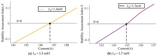
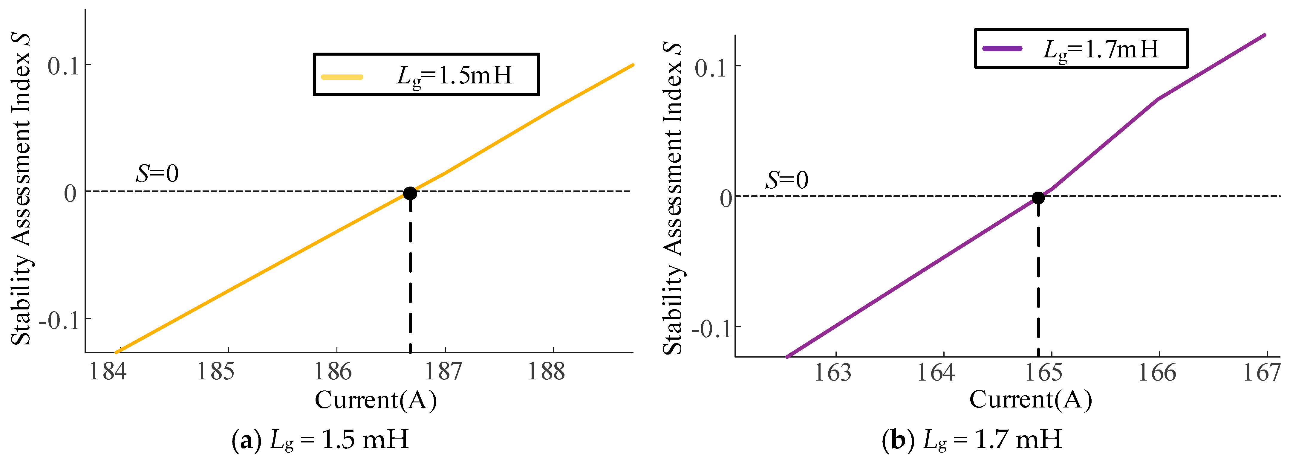
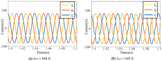
To further validate the accuracy of the proposed method in characterizing the stable operating boundary, enlarged prediction results of the stable operating boundary for Lg = 1.5 mH and Lg = 1.7 mH are presented in Figure 11. As shown in Figure 11, when Lg = 1.5 mH, the critical stable current predicted by the stability assessment model is 186 A. When Lg = 1.7 mH, the predicted critical stable current is 164 A.
Figure 11.
Stable operating boundaries under different grid inductances.
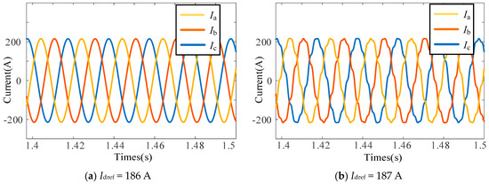
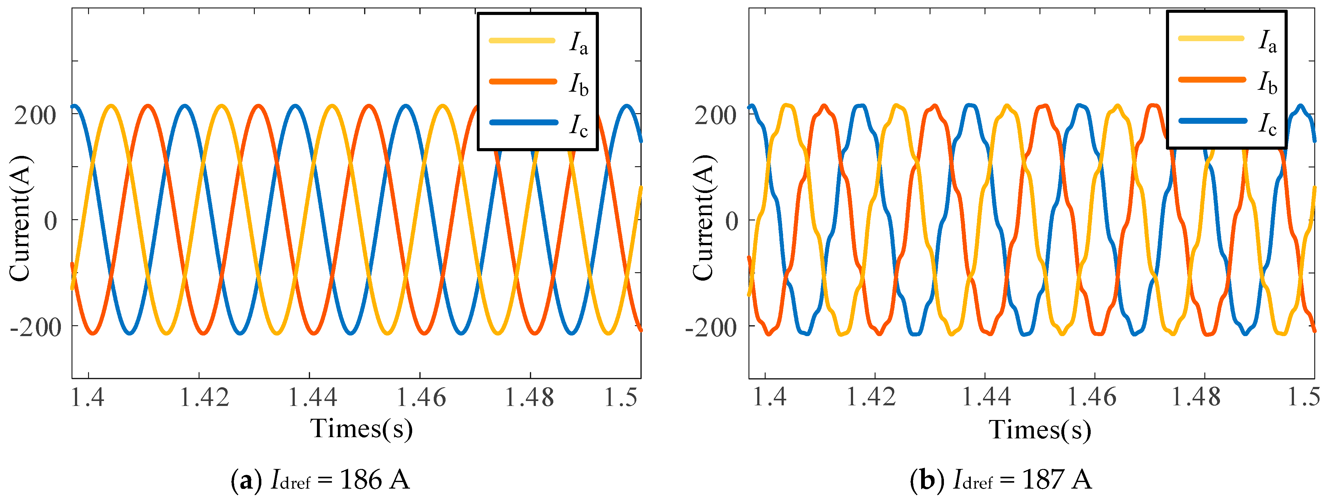
Figure 12 presents the PCC current waveforms when Lg = 1.5 mH and the current reference is set around the predicted critical current. As shown in Figure 12, when Idref is set to 186 A, the current remains sinusoidal, indicating that the system is stable. When Idref is increased to 187 A, obvious waveform distortion and oscillations appear in the current, indicating that the system becomes unstable. Similarly, Figure 13 shows the PCC current waveforms when Lg = 1.7 mH and the current reference is also set around the predicted critical current. When Idref is increased from 164 A to 165 A, the system transitions from a stable state to an unstable state. According to the analysis in Figure 11 and Figure 12, the error of the predicted stability boundary is less than 1 A, that is, the prediction error is less than 1 A/400 A = 0.25%. The time-domain simulation results are consistent with the prediction results of the stability assessment model. Once the operating point exceeds the predicted critical stable operating point, the system changes from stable operation to an oscillatory state.
Figure 12.
Current waveforms and total harmonic distortion under Lg = 1.5 mH.
Figure 13.
Current waveforms and total harmonic distortion under Lg = 1.7 mH.
The above simulation results demonstrate that the BP neural network-based stability assessment model can rapidly and accurately evaluate the stability of the grid-connected converter system under different operating conditions. Moreover, the stable operating boundary of the system under different grid impedances can be accurately predicted. Therefore, the proposed method provides effective technical support for online small-signal stability assessment and operational risk warning of the grid-connected converter system.
5. Conclusions
For the small-signal stability problem introduced by black-box grid-connected converters, a small-signal stability assessment method is proposed by combining offline impedance measurement, the GNC, and a BP neural network. The main conclusions, contributions and limitations are summarized as follows:
- (1)
- Both converter operating points and grid impedance variations affect the system stability margin. The stability margin gradually decreases as the output current or grid impedance increases.
- (2)
- The magnitude of the impedance ratio matrix eigenvalue at the phase of −180 degrees is proposed as a quantitative stability assessment index. In this way, the system stability assessment is transformed from a binary stable/unstable judgment to a continuous stability margin characterization. This index provides physically meaningful output labels for data-driven model training.
- (3)
- Guided by prior knowledge from analytical stability assessment, a BP neural network-based stability assessment model is constructed. Bayesian regularization is used to constrain the model complexity. On this basis, the stable operating boundary of the grid-connected converter system is characterized. Simulation results show that the proposed method can rapidly and accurately reflect the stability of the grid-connected converter system, and the prediction error of the stability boundary is less than 0.25%.
- (4)
- The applicability of the proposed BP neural network is limited by the range of the training data. For operating conditions beyond the predefined training range, additional samples are required to extend the applicable range of the stability assessment model.
Author Contributions
Conceptualization, Q.Y.; methodology, X.L.; software, Y.X.; validation, X.L., and Y.X.; formal analysis, L.L.; resources, Q.Y. and X.Z.; data curation, Y.H.; writing—original draft preparation, M.N. and H.X.; writing—review and editing, Y.H., Q.Y. and X.Z.; visualization, H.X.; supervision, Q.Y.; project administration, Q.Y.; funding acquisition, X.L. All authors have read and agreed to the published version of the manuscript.
Funding
This work was supported by the Science and Technology Project of State Grid Sichuan Electric Power Company, titled “Source-Storage Coordinated Planning Technology for Power Supply Transmission Channels Considering Synchronous Stability”, ERP number 52199625000F.
Data Availability Statement
The original contributions presented in this study are included in the article. Further inquiries can be directed to the corresponding author.
Conflicts of Interest
Authors Qiang Ye, Xuehai Lv, Yueping Xiang, Luoyi Li, and Yanqiu Hou were employed by the Economic and Technical Research Institute of State Grid Sichuan Electric Power Company. The remaining authors declare that the research was conducted in the absence of any commercial or financial relationships that could be construed as a potential conflict of interest. The authors declare that this study received funding from the Economic and Technical Research Institute of State Grid Sichuan Electric Power Company. The funder was not involved in the study design; the collection, analysis, or interpretation of data; the writing of this article; or the decision to submit it for publication.
Abbreviations
The following abbreviations are used in this manuscript:
| GNC | Generalized Nyquist criterion |
| BP | Backpropagation |
| PCC | Point of common coupling |
| PLL | Phase-locked loop |
| THD | Total harmonic distortion |
Appendix A
Table A1.
Main parameters of the grid-connected converter system.
References
- National Energy Administration. National Energy Administration Releases National Power Industry Statistics for 2025 [EB/OL]; National Energy Administration: Beijing, China, 2026.
- Ma, N.; Xie, X.; He, J.; Wang, H. Review of wide-band oscillation in renewable and power electronics highly integrated power systems. Proc. CSEE 2020, 40, 4720–4732. [Google Scholar]
- Strachan, N.P.W.; Jovcic, D. Stability of a variable-speed permanent magnet wind generator with weak AC grids. IEEE Trans. Power Deliv. 2010, 25, 2779–2788. [Google Scholar] [CrossRef] [Scilit]
- Huang, Y.; Yuan, X.; Hu, J.; Zhou, P. Modeling of VSC connected to weak grid for stability analysis of DC-link voltage control. IEEE J. Emerg. Sel. Top. Power Electron. 2015, 3, 1193–1204. [Google Scholar] [CrossRef] [Scilit]
- Mouton, D.A.; Mararakanye, N.; Bekker, B. Assessment of methods to measure power system flexibility: A review. In Proceedings of the 2021 56th International Universities Power Engineering Conference (UPEC), Middlesbrough, UK, 31 August–3 September 2021; pp. 1–6. [Google Scholar]
- Zou, H.; Xing, Q.; Fu, H.; Zhang, T.; Chen, Y.; Zhu, J. Enhancing distribution network flexibility via adjustable carbon emission factors and negative-carbon incentive mechanism. Processes 2025, 13, 4023. [Google Scholar] [CrossRef] [Scilit]
- Yang, H.; Chen, Q.; Tang, K.; Zhang, D.; Shen, Y. Flexibility aggregation and cooperative scheduling for distributed resources using a virtual battery equivalence technique. Energy 2025, 334, 137770. [Google Scholar] [CrossRef] [Scilit]
- Pogaku, N.; Prodanovic, M.; Green, T.C. Modeling, analysis and testing of autonomous operation of an inverter-based microgrid. IEEE Trans. Power Electron. 2007, 22, 613–625. [Google Scholar] [CrossRef] [Scilit]
- Bottrell, N.; Prodanovic, M.; Green, T.C. Dynamic stability of a microgrid with an active load. IEEE Trans. Power Electron. 2013, 28, 5107–5119. [Google Scholar] [CrossRef] [Scilit]
- Rasheduzzaman, M.; Mueller, J.A.; Kimball, J.W. An accurate small-signal model of inverter-dominated islanded mcrogrids using dq reference frame. IEEE J. Emerg. Sel. Top. Power Electron. 2014, 2, 1070–1080. [Google Scholar] [CrossRef] [Scilit]
- Wang, Y.; Wang, X.; Blaabjerg, F.; Chen, Z. Harmonic instability assessment using state-space modeling and participation analysis in inverter-fed power systems. IEEE Trans. Ind. Electron. 2017, 64, 806–816. [Google Scholar] [CrossRef] [Scilit]
- Cespedes, M.; Sun, J. Impedance modeling and analysis of grid-connected voltage-source converters. IEEE Trans. Power Electron. 2014, 29, 1254–1261. [Google Scholar] [CrossRef] [Scilit]
- Wen, B.; Boroyevich, D.; Burgos, R.; Mattavelli, P.; Shen, Z. Analysis of D-Q small-signal impedance of grid-tied inverters. IEEE Trans. Power Electron. 2016, 31, 675–687. [Google Scholar] [CrossRef] [Scilit]
- Sun, J. Impedance-based stability criterion for grid-connected inverters. IEEE Trans. Power Electron. 2011, 26, 3075–3078. [Google Scholar] [CrossRef] [Scilit]
- Bakhshizadeh, M.K.; Wang, X.; Blaabjerg, F.; Kocewiak, L.; Bak, C.L.; Hesselbæk, B. Couplings in phase domain impedance modeling of grid-connected converters. IEEE Trans. Power Electron. 2016, 31, 6792–6796. [Google Scholar] [CrossRef] [Scilit]
- Xin, H.; Li, Z.; Dong, W.; Wang, Z.; Zhang, L. A generalized-impedance based stability criterion for three-phase grid-connected voltage source converters. arXiv 2017, arXiv:1703.10514. [Google Scholar]
- Shen, Z.; Jaksic, M.; Mattavelli, P.; Boroyevich, D.; Verhulst, J.; Belkhayat, M. Three-phase AC system impedance measurement unit using chirp signal injection. In Proceedings of the IEEE Applied Power Electronics Conference and Exposition (APEC), Long Beach, CA, USA, 17–21 March 2013; pp. 2666–2673. [Google Scholar]
- Roinila, T.; Messo, T.; Santi, E. MIMO-identification techniques for rapid impedance-based stability assessment of three-phase systems in DQ domain. IEEE Trans. Power Electron. 2018, 33, 4015–4022. [Google Scholar] [CrossRef] [Scilit]
- You, S.; Zhao, Y.; Mandich, M.; Cui, Y.; Li, H.; Xiao, H.; Fabus, S.; Su, Y.; Liu, Y.; Yuan, H. A review on artificial intelligence for grid stability assessment. In Proceedings of the IEEE International Conference on Communications, Control, and Computing Technologies for Smart Grids (Smart Grid Comm), Tempe, AZ, USA, 11–13 November 2020; pp. 1–6. [Google Scholar]
- Zhang, M.; Wang, X.; Yang, D.; Christensen, M.G. Artificial neural network based identification of multi-operating-point impedance model. IEEE Trans. Power Electron. 2021, 36, 1231–1235. [Google Scholar] [CrossRef] [Scilit]
- Wu, B.; Li, J.; Li, Y.; Wang, Y.; Liu, Q.; Yang, Y. Knowledge-and-data-driven impedance acquisition for grid-connected inverters under multiple operating conditions. Autom. Electr. Power Syst. 2022, 46, 83–91. [Google Scholar]
- Zhu, L.; Hill, D.J.; Lu, C. Hierarchical deep learning machine for power system online transient stability prediction. IEEE Trans. Power Syst. 2020, 35, 2399–2411. [Google Scholar] [CrossRef] [Scilit]
- Zhang, D.; Yang, Y.; Shen, B.; Wang, T.; Cheng, M. Transient stability assessment in power systems: A spatiotemporal graph convolutional network approach with graph simplification. Energies 2024, 17, 5095. [Google Scholar] [CrossRef] [Scilit]
- Tu, C.; Gao, J.; Xiao, F.; Guo, Q.; Jiang, F. Stability Analysis of the Grid-Connected Inverter Considering the Asymmetric Positive-Feedback Loops Introduced by the PLL in Weak Grids. IEEE Trans. Ind. Electron. 2022, 69, 5793–5802. [Google Scholar] [CrossRef] [Scilit]
- Guo, B.; Zhang, X.; Ma, H.; Yang, Y.; Wang, X.; Tian, Q.; Jin, S. A Series Impedance Reshaping Control Method Considering PLL Dynamics for Grid-Connected Inverters Under Weak Grid Conditions. IEEE Trans. Ind. Electron. 2024, 71, 4896–4910. [Google Scholar] [CrossRef] [Scilit]
- Mohammed, N.; Ciobotaru, M.; Town, G. Fundamental grid impedance estimation using grid-connected inverters: A comparison of two frequency-based estimation techniques. IET Power Electron. 2020, 13, 2730–2741. [Google Scholar] [CrossRef] [Scilit]
- Ghanem, A.; Rashed, M.; Sumner, M.; Elsayes, M.A.; Mansy, I.I.I. Grid impedance estimation for islanding detection and adaptive control of converters. IET Power Electron. 2017, 10, 1279–1288. [Google Scholar] [CrossRef] [Scilit]

Disclaimer/Publisher’s Note: The statements, opinions and data contained in all publications are solely those of the individual author(s) and contributor(s) and not of MDPI and/or the editor(s). MDPI and/or the editor(s) disclaim responsibility for any injury to people or property resulting from any ideas, methods, instructions or products referred to in the content. |
© 2026 by the authors. Licensee MDPI, Basel, Switzerland. This article is an open access article distributed under the terms and conditions of the Creative Commons Attribution (CC BY) license.