Transmission Characteristics and Machine Learning Prediction of Lateral Vibration in Deep Vertical Drill Strings

Abstract

Severe drill string vibration can accelerate tool fatigue and failure, but direct measurement near the drill bit is difficult. Using a 6376 m vertical shale-gas well in western Sichuan as a case study, this study established and validated a coupled drill string dynamic model. Lateral acceleration signals under three operating conditions were generated, filtered, and normalized. XGBoost models were then trained using vibration signals measured at shallow and intermediate locations to estimate deep-level lateral acceleration. The results showed that vibration originated near the drill bit and propagated upward with a measurable delay, while its amplitude was generally higher in the middle section of the drill string. For single-point monitoring, the coefficient of determination (R²) ranged from 0.013 at 500 m to 0.64 at 10 m from the bit. Combining multiple monitoring locations increased R² to 0.7071. XGBoost achieved the best balance between accuracy and computational efficiency among the tested models. The 10–300 m interval from the bit is recommended for monitoring, whereas 300–500 m is considered an uncertain zone.

1. Introduction

Petroleum and natural gas are critical strategic fossil-fuel resources closely related to national security and economic development [1,2,3]. Drilling is one of the crucial phases of hydrocarbon exploitation. During drilling operations, the drill string is subjected to multiple factors, such as bottomhole pressure, formation-temperature variations, and changes in rock hardness, which generate various forms of vibration. These vibrations inevitably induce fatigue failure of the drill string. Statistical data indicate that global economic losses attributed to drill string failures reach billions of dollars annually [4]. The excessive length of the drill string results in greater flexibility and lower stiffness, readily triggering low-frequency, large-amplitude vibrations [5,6,7]. Furthermore, the intense combined loads exerted by waves, ocean currents, and high-pressure/low-temperature (HP/LT) environments facilitate multimodal coupling among axial, lateral, and torsional vibrations, frequently inducing bending deformation of the drill string [8,9]. Consequently, the control of drill string vibration is highly prioritized by both academia and industry, and related research has been conducted extensively.

Lubinski et al. [10] established the “soft-string model” based on the Euler–Bernoulli beam theory and derived differential equations governing the force and deformation behavior of axial drill string vibrations, laying a solid foundation for research on drill string statics and dynamics. Finnie and Bailey [11] initially obtained approximate solutions for the natural frequencies of the drill string under undamped conditions by combining experimental methods with a trial-and-error approach. This work was crucial to the development of early drill string dynamic models. Dareing and Livesay [12] established the equations of motion for the entire drill string system and incorporated damping effects, successfully demonstrating the feasibility of predicting drill string life. As the understanding of multiple downhole vibration modes—such as lateral, axial, torsional, whirling, and stick–slip vibrations—and their complex coupling has progressively deepened, scholars worldwide have made substantial breakthroughs in establishing drill string dynamic models and investigating nonlinear problems. Millheim et al. [13] extended the finite-element method (FEM) from two to three dimensions and pioneered its application to drill string vibration analysis, providing numerical tools that closely represent actual operating conditions. Furthermore, Zhang et al. [14] focused on developing experimental apparatus and successfully constructed the first domestic motion-simulation device for the bottomhole assembly (BHA). Their findings laid a solid foundation for experimental studies of drill string dynamics in China. While investigating the influence of upper and lower boundary conditions on drill string vibrations, Clayer et al. [15] simplified the entire drilling system into a “mass–spring–damper” system and concluded that borehole wall collisions and drilling fluid damping have the greatest impact on the critical vibration threshold. Liu [16] combined the Wilson-θ and Newton–Raphson methods to effectively analyze and solve two nonlinear problems: the axial–lateral geometric nonlinearity of the drill string and the contact nonlinearity involving different borehole wall materials. Consequently, a three-dimensional nonlinear finite-element model was successfully constructed. Remmert [17] proposed a geometrically nonlinear model to comprehensively investigate the coupling between axial and torsional vibrations along the drill string. In this model, the drill string is accurately described as a vertical slender beam undergoing axial rotation, and large rotations and nonlinear strain–displacement relationships were rigorously considered. Preliminary analysis indicates that the linear and nonlinear models diverge significantly after the initial stick–slip phase. This dynamic behavior becomes prominent as friction beneath the drill bit increases. Based on actual wellbore trajectories and considering collisions between the drill string and the borehole wall, Di et al. [18] comprehensively characterized the dynamics of the entire drill string through finite-element simulation. In complex formations, the mechanical boundary conditions imposed on the drill string are also affected by the coupled response of the surrounding formation. Fan et al. [19] developed analytical solutions for a semipermeable wellbore subjected to convective cooling and nonhydrostatic in situ stresses within a fully coupled thermoporoelastic framework. Their results showed that the assumed permeability of the borehole wall can significantly affect the transient distributions of temperature, pore pressure, and stress around the wellbore. More recently, Li et al. [20] extended this type of analysis to a transversely isotropic thermoporoelastic medium under nonhydrostatic in situ stresses and convective boundary conditions. These studies demonstrate that formation anisotropy, thermal perturbations, fluid transport, and nonhydrostatic stresses may jointly affect borehole deformation and stability. Such changes may, in turn, modify the clearance and contact conditions between the drill string and borehole wall, thereby influencing the lateral dynamic response of the drill string.

The computational cost of numerically simulating drill string vibrations Increases considerably with well depth and well-profile complexity. Given its high computational efficiency and capacity for processing massive datasets, machine learning has rapidly emerged as a novel approach to investigating drill string vibrations. Using wavelet functions to select appropriate scale and translation parameters, Zhang [21] successfully constructed a wavelet neural network based on a single-scale tight frame. Using common drilling accidents—namely, lost circulation and well kicks—as case studies, the network parameters were effectively trained. Consequently, this network reliably evaluates drilling accidents with an accuracy exceeding 96%. Zhu et al. [22] accurately extracted local-scale drill string vibration features in the time and frequency domains and subsequently used wavelet analysis to explore data-driven machine learning optimization of dynamic parameters. During field-development operations, the resulting vibration early-warning mechanisms successfully reduced the failure rate of drilling tools by 40%. Yi et al. [23] proposed an improved adaptive genetic algorithm (AGA) and established an innovative nonlinear optimization model. Saadeldin et al. [24] constructed an intelligent vibration prediction model driven by surface parameters and based on the random forest machine learning algorithm, enabling instantaneous diagnosis of downhole vibrations in horizontal wells. Requiring only parameters such as weight on bit (WOB), rotary speed (RPM), surface torque, and mud-flow rate, this model effectively predicts downhole high-frequency torsional oscillations (HFTOs). Furthermore, its test-set accuracy reaches 89%, outperforming a series of conventional physics-based models represented by finite-element simulations by approximately 30%. Huang et al. [25] successfully constructed an early-warning model for stick–slip events using a long short-term memory (LSTM) neural network. By performing time-series analysis using 150 s of historical measurements and 193 s of triaxial acceleration data, the model accurately identifies stick–slip events through sliding-window calculations. Consequently, it issues warnings 3 min in advance, substantially enhancing the safety margin of downhole operations. Zhang et al. [26] comprehensively summarized applications of various algorithms—including support vector regression (SVR), random forest, and neural networks—to drilling-condition identification, which consistently achieved high accuracy. Chen et al. [27] proposed an innovative hybrid prediction model integrating three architectures: physics-informed neural networks (PINNs), fusion neural networks (NNs), and long short-term memory (LSTM) networks. This technology has been successfully applied to actual drilling operations in the Fuman block of the Tarim Oilfield.

Existing machine learning studies on drill string dynamics have mainly focused on vibration-state identification, drilling-dysfunction classification, or the prediction of drilling responses from surface measurements and operating parameters. However, limited attention has been paid to the spatial relationship between vibration signals measured at different locations along a deep drill string and its implications for monitoring location selection. Moreover, because direct and continuous measurement near the drill bit remains difficult, a method for estimating deep-level vibration from signals acquired at more accessible locations is required.

Unlike conventional machine learning approaches aimed at future-time forecasting, the present study establishes a same-time-point spatial mapping between lateral acceleration signals at different locations along the drill string. Specifically, the signals measured at selected shallow and intermediate locations at time t are used to estimate the deep-level lateral acceleration at the same time t; therefore, the prediction horizon is zero. The proposed framework combines a validated coupled drill string dynamic model, Fourier low-pass filtering, and machine learning-based regression to investigate how the estimation performance varies with monitoring distance from the drill bit.

The main scientific contributions of this study are threefold. First, a spatially distributed drill string vibration database is constructed using a coupled dynamic model validated against experimental observations. Second, the relationship between monitoring location and deep-level lateral vibration estimation performance is quantitatively evaluated, providing a data-driven characterization of the spatial observability of drill string vibration. Third, the location-dependent estimation results are translated into recommended, uncertain, and nonrecommended monitoring zones, thereby providing a quantitative basis for selecting downhole vibration-monitoring locations. Thus, the contribution of this study lies not in developing a new machine learning algorithm but in integrating drill string dynamics with data-driven spatial estimation to support indirect bottomhole vibration assessment and monitoring location selection.

2. Preliminary Analysis of the Database

2.1. Validation of the Numerical Simulation

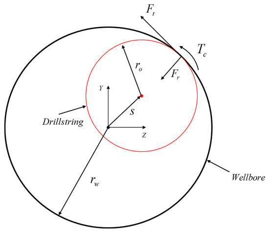
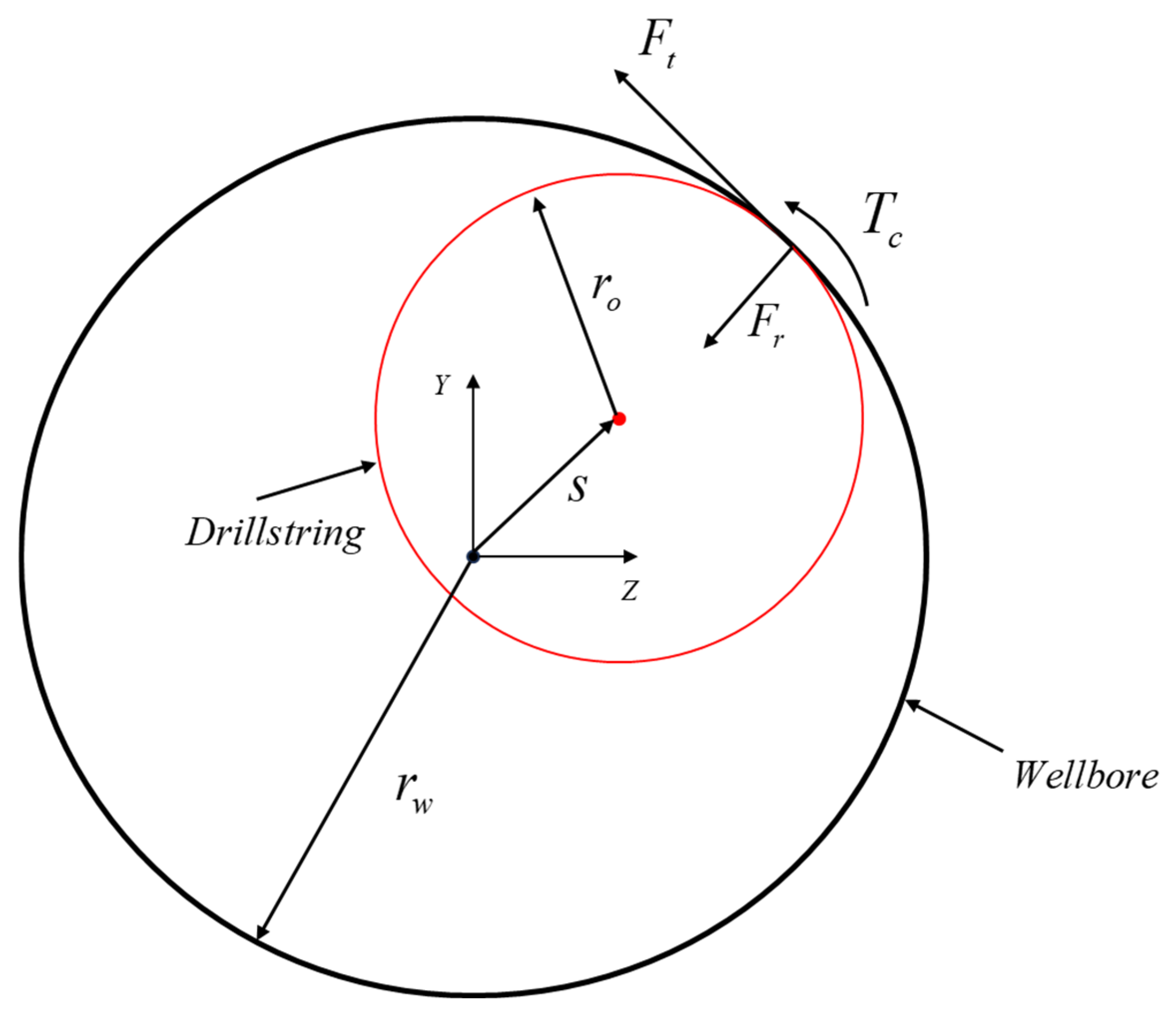
Using a nonlinear finite-element method with large-rotation vectors, this study establishes a dynamic model of the entire drill string system to accurately simulate drill string vibration. The top of the drill string is subjected to a large axial load, fixed laterally, and driven torsionally at a fixed rotational speed. The bottom is axially free and supported laterally by an elastic support, while its torsional motion is affected by friction. A penalty function is used to represent the contact force between the drill string and the borehole wall. The penalty functions are shown in Equations (1)–(3), and the contact model is depicted in Figure 1.

$$F_{contact}=\left\{\begin{array}{l}-K_{contact}(u_r-\frac{D_{well}-D_{string}}{2})\\ 0\end{array}\right.$$

(1)

$$F_f=\mu F_{contact}$$

(2)

$$F_{torq}=\frac{D_{string}}{2}{F}_f$$

(3)

where

Figure 1. Drill string–wellbore contact plot.

• $F_{contact}$ represents the contact force, $\mathrm{N}$;
• $K_{contact}$ represents the contact stiffness of well wall, $\mathrm{N}/\mathrm{m}$;
• $u_r$ represents the displacement of the wellbore wall, $m$;
• $D_{well}$ is the diameter of the wellbore wall, and $D_{string}$ is the outer diameter of the drill string, $m$;
• $F_f$ represents the frictional force between the well wall and drill string, $\mathrm{N}$;
• $\mu$ represents the coefficient of friction;
• $F_{torq}$ represents the contact torque, N·m.

Consequently, the relationship between operating parameters and drill string vibration is established, systematically forming a drill string dynamics database. This method effectively discretizes the drill string, which has a large slenderness ratio, into viscoelastic beam elements while comprehensively considering nonlinear conditions, including deformation, elastoplasticity, variations in contact forces, and buckling instability of the drill string.

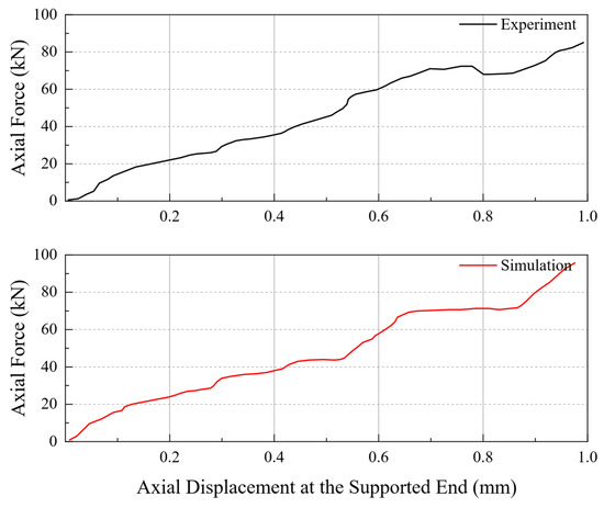
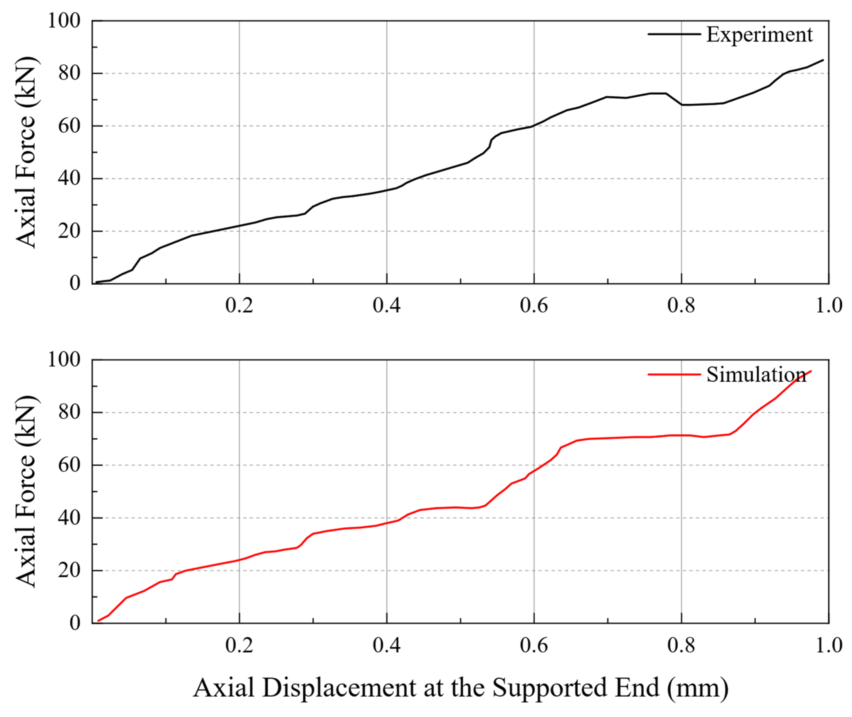
Song [28] verified the model’s accuracy in calculating the response of a cylinder under combined forces by rigorously comparing the results of an on-site simulation experiment with those of a numerical simulation based on the aforementioned framework. Song innovatively used a hollow cylindrical plastic rod to simulate the wellbore and a copper rod to simulate the drill string. Furthermore, axial forces and displacements were measured using force and displacement sensors, respectively. The axial force–displacement relationship of the copper rod during the transition from sinusoidal to helical buckling was meticulously recorded. Simultaneously, the experimental parameters were entered into the drill string dynamic model to obtain the axial force–displacement relationship of the drill string. Figure 2 plots the experimental data and simulation results in the same coordinate system.

Figure 2. Comparison of axial force–displacement curves between the experiment and model simulation.

A comprehensive comparison reveals that the simulation results calculated by the model closely align with the experimental observations, demonstrating the high accuracy of the model. To quantitatively evaluate the consistency between the simulation and experimental results, three statistical metrics were calculated for the full axial force–displacement curve covering the entire buckling process. The coefficient of determination (R²) between the simulated and experimental curves reaches 0.987, the mean relative error is 2.41%, and the maximum relative error is 4.68%. The comprehensive comparison reveals that the simulation results calculated by the model closely align with the experimental observations, demonstrating the high accuracy of the model in capturing the nonlinear mechanical behavior of slender rod strings.

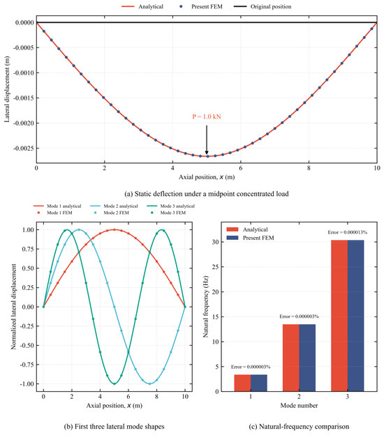
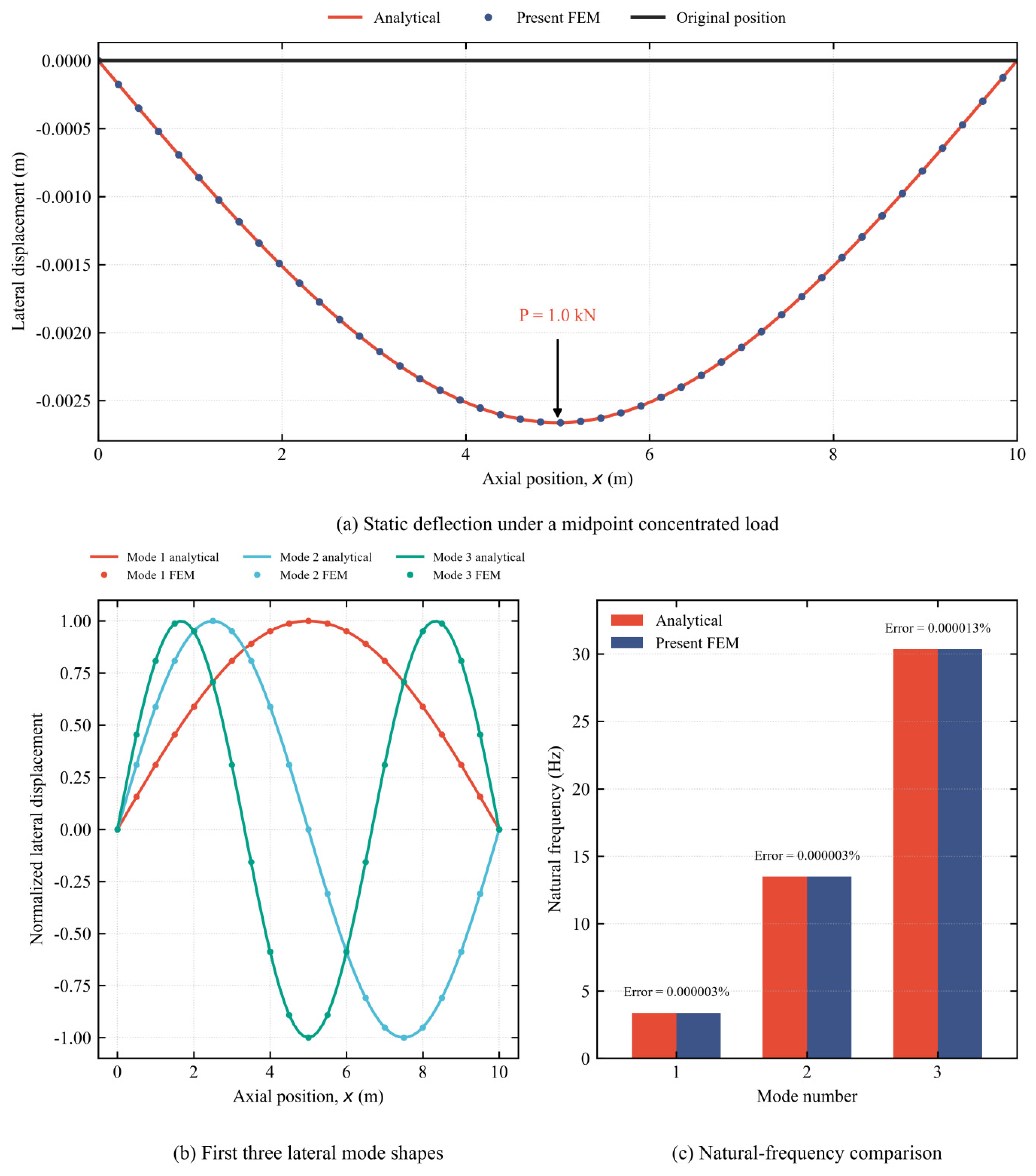
To further verify the finite-element formulation, a uniform simply supported the Euler–Bernoulli beam with a length of 10 m was discretized into 80 elements. The element bending-stiffness and consistent mass matrices were identical to those used in the drill string solver. The static deflection under a 1.0 kN midpoint concentrated load was first compared with the corresponding closed-form solution. Subsequently, the first three natural frequencies and normalized lateral mode shapes obtained from the finite-element model were compared with the analytical solutions. The specific results are shown in Figure 3.

Figure 3. Analytical verification of the finite-element formulation using a simply supported uniform beam.

The analytical and finite-element deflection curves were nearly coincident, and the relative error in the midpoint deflection was less than 1.0 × 10⁻⁸. The analytical natural frequencies of the first three modes were 3.37165238, 13.48660954, and 30.34487146 Hz, whereas the corresponding finite-element results were 3.37165249, 13.48660988, and 30.34487551 Hz. The relative errors were 0.000003%, 0.000003%, and 0.000013%, respectively. The close agreement verifies the implementation of the bending-stiffness matrix, consistent mass matrix, boundary conditions, and generalized eigenvalue solution under idealized linear conditions.

2.2. Parameters of Wellbore Structure

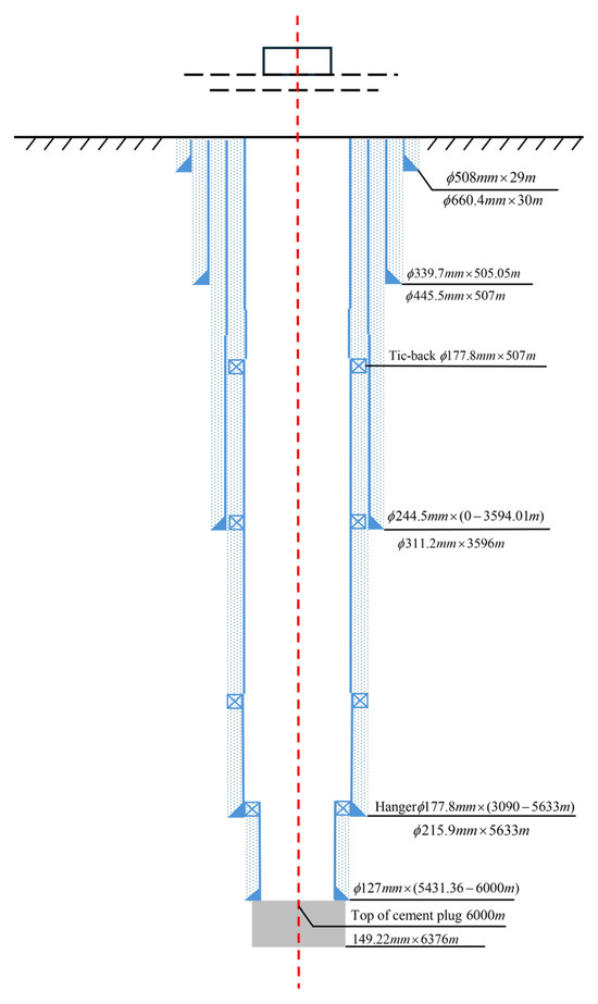
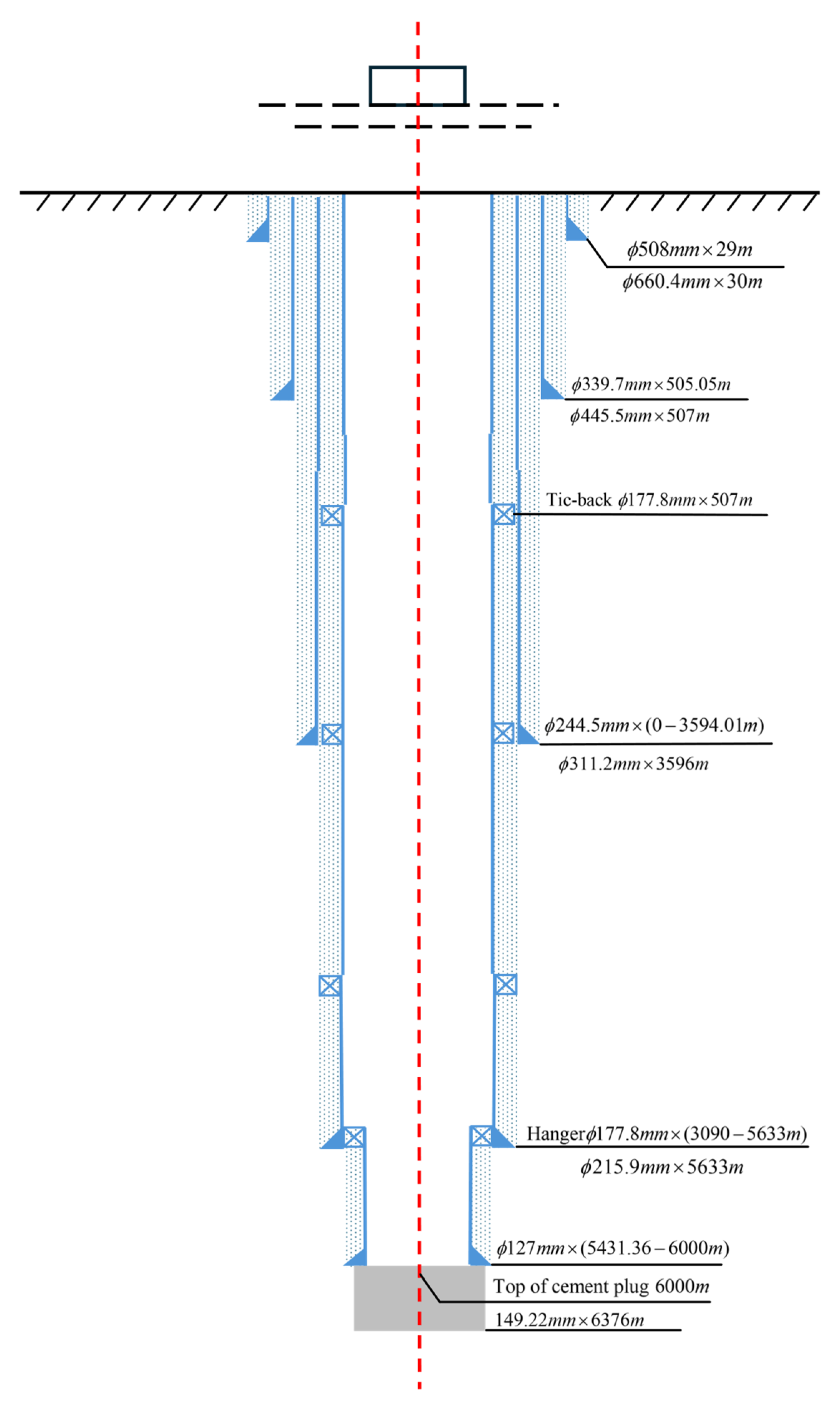
A well in the western Sichuan gas field is used as the subject of the simulation analysis in this study, and its wellbore design is detailed as follows:

From depths of 0 to 29 m, a conductor section with an internal diameter of 20 in. (508 mm) is installed to prevent wellhead collapse and shallow fluid erosion, provide guidance and a foundation for installing lower casing strings, and support most of the gravitational load.

From depths of 29 to 500 m, a technical casing string with an internal diameter of 13.37 in. (339.7 mm) is installed through shallow aquifers and into stable bedrock to prevent drilling fluid loss and wellbore wall collapse and to provide an anchoring point for subsequent technical casing strings.

From depths of 0 to 3594 m, an intermediate casing string with an internal diameter of 9.64 in. (244.5 mm) is installed to isolate high-pressure and collapse-prone formations at intermediate depths, prevent blowouts, and stabilize the borehole wall.

From depths of 3090 to 5633 m, a liner with an internal diameter of 7 in. (177.8 mm) is installed to accommodate the drill bit dimensions required for subsequent operations and improve reservoir fluid flow efficiency. A uniform friction coefficient of 0.4 is adopted for the entire wellbore section, greatly simplifying the computational model for frictional drag. A schematic of the wellbore structure is shown in Figure 4.

Figure 4. Schematic plot of the wellbore structure.

Based on the wellbore structure and historical drilling records, this study uses the bottomhole assembly employed while drilling the measured-depth interval from 6372.60 to 6376.00 m as the assembly for numerical simulation to accurately reproduce drill string vibration in deep formations. The drill string assembly is presented in Table 1.

Table 1. Drill string assembly.

Name of Drill Tool × Specification and Model	Outer Diameter (mm)	Inner Diameter (mm)	Length (m)	Cumulative Length (m)
Roller cone bit × HJT537GK	149.20	-	0.18	0.18
Crossover sub	-	-	0.58	0.76
Check valve	-	-	0.40	1.16
Spiral drill collar × 5 H-90	120.70	57.15	81.15	82.31
Crossover sub	-	-	0.42	82.73
Drill pipe × S135I	101.60	70.21	6293.27	6376.00

2.3. Dynamic Analysis of the Drill String

Due to the moderate abrasiveness of the reservoir dolomite, an HJT537GK roller cone bit was used in the field operation. The operating parameters were determined by considering the formation characteristics, the recommended operating range of the bit, and historical drilling records. The WOB was maintained within the range of 30–80 kN, while the rotary speed was adjusted between 60 and 150 r/min according to lithological variations. A relatively high rotary speed was used in formations with better drilling ability, whereas the rotary speed was reduced when mudstone or shale interbeds were encountered to mitigate periodic impact loads and control drill string vibration [29]. Based on the recorded operating parameters, three combinations of WOB and rotary speed were selected as representative operating conditions for comparative analysis, as listed in Table 2.

Table 2. Comparison of operating parameters.

Working Condition	Weight on Bit (kN)	Rotary Speed (r/min)
1	50 kN	70 r/min
2	36 kN	60 r/min
3	40 kN	80 r/min

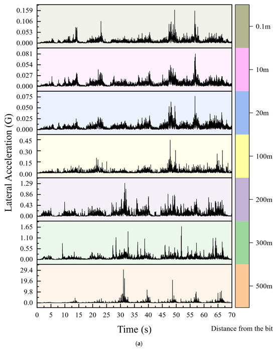
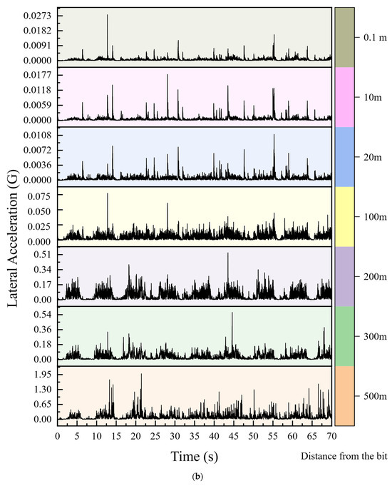
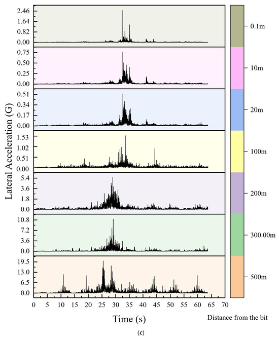
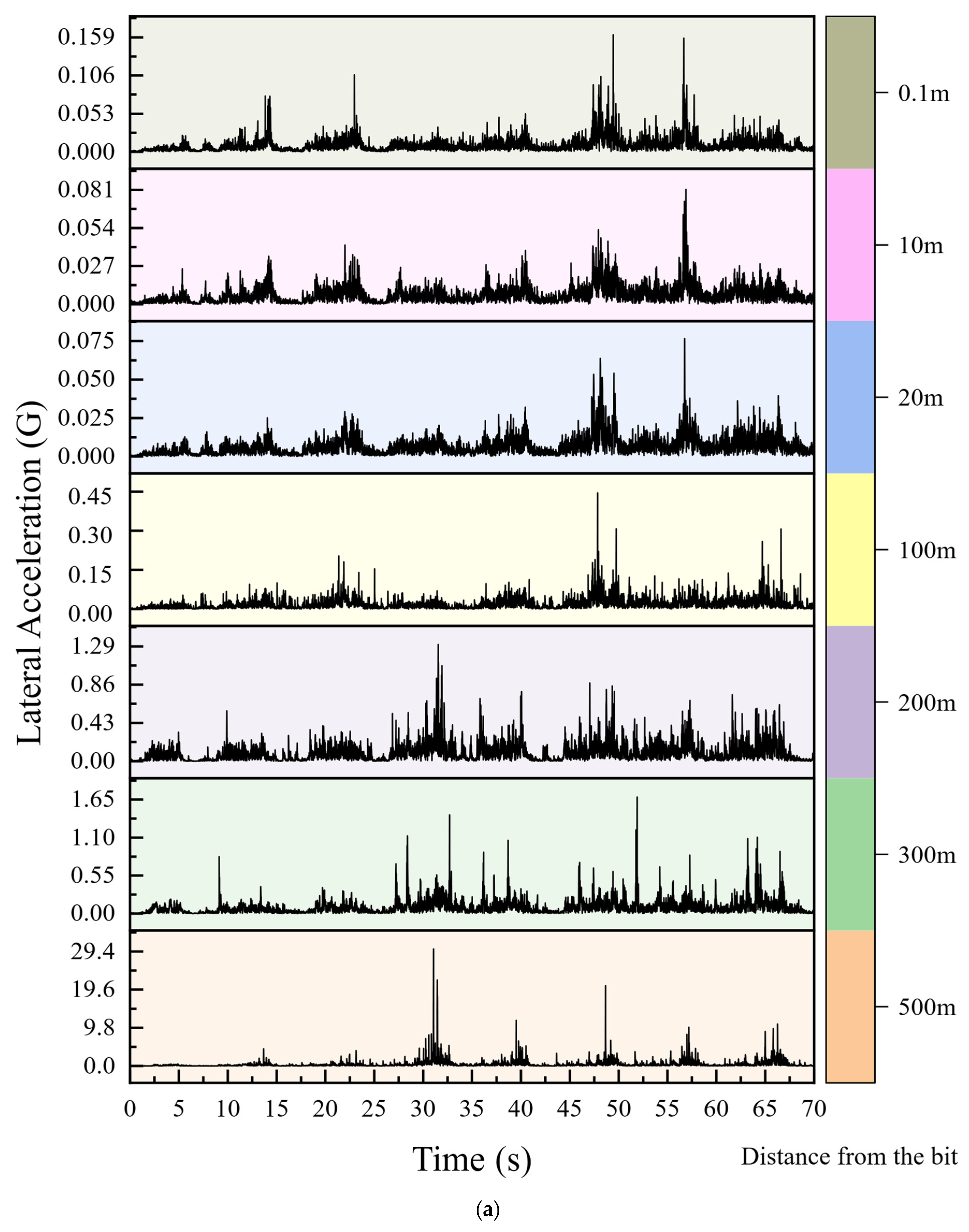
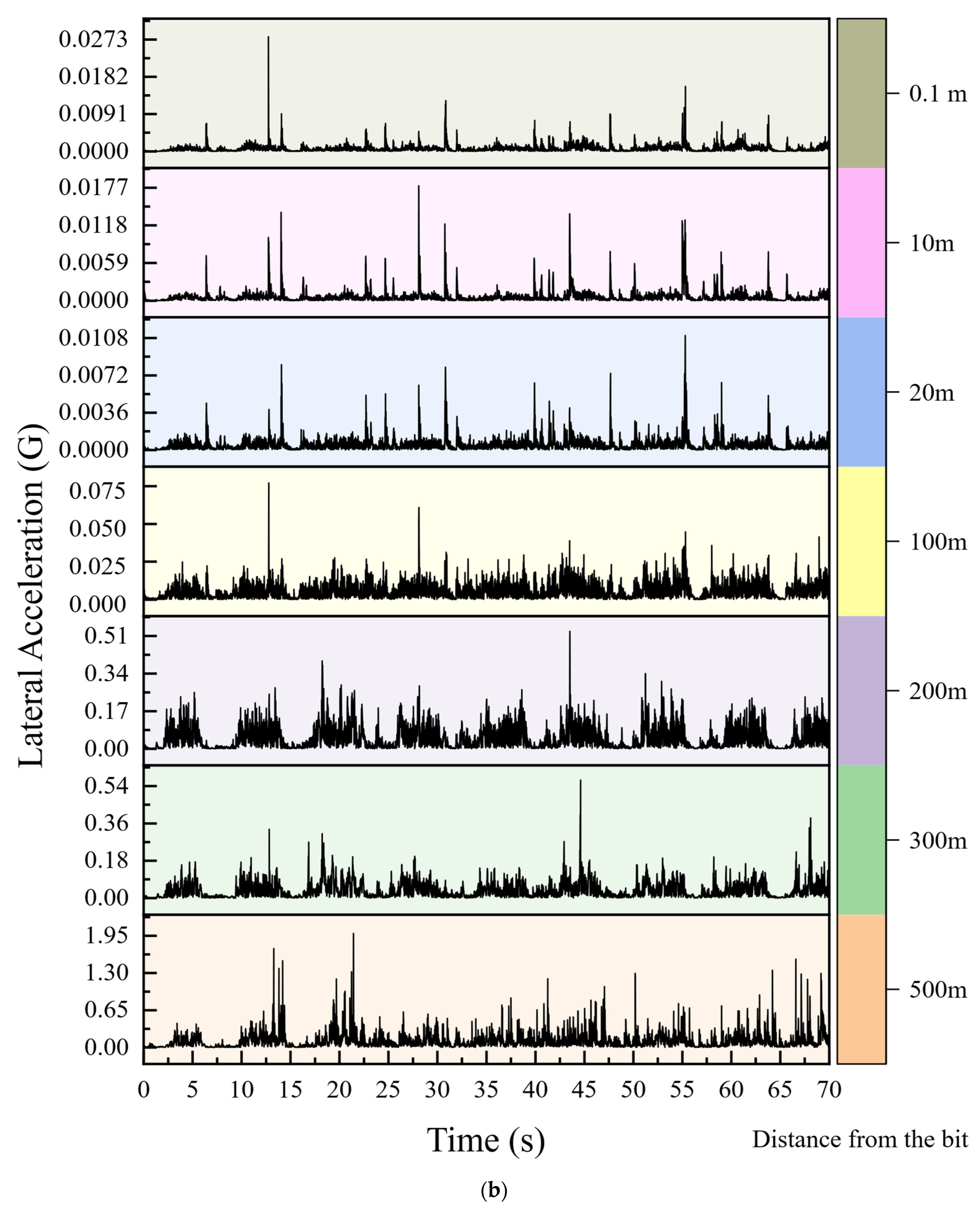
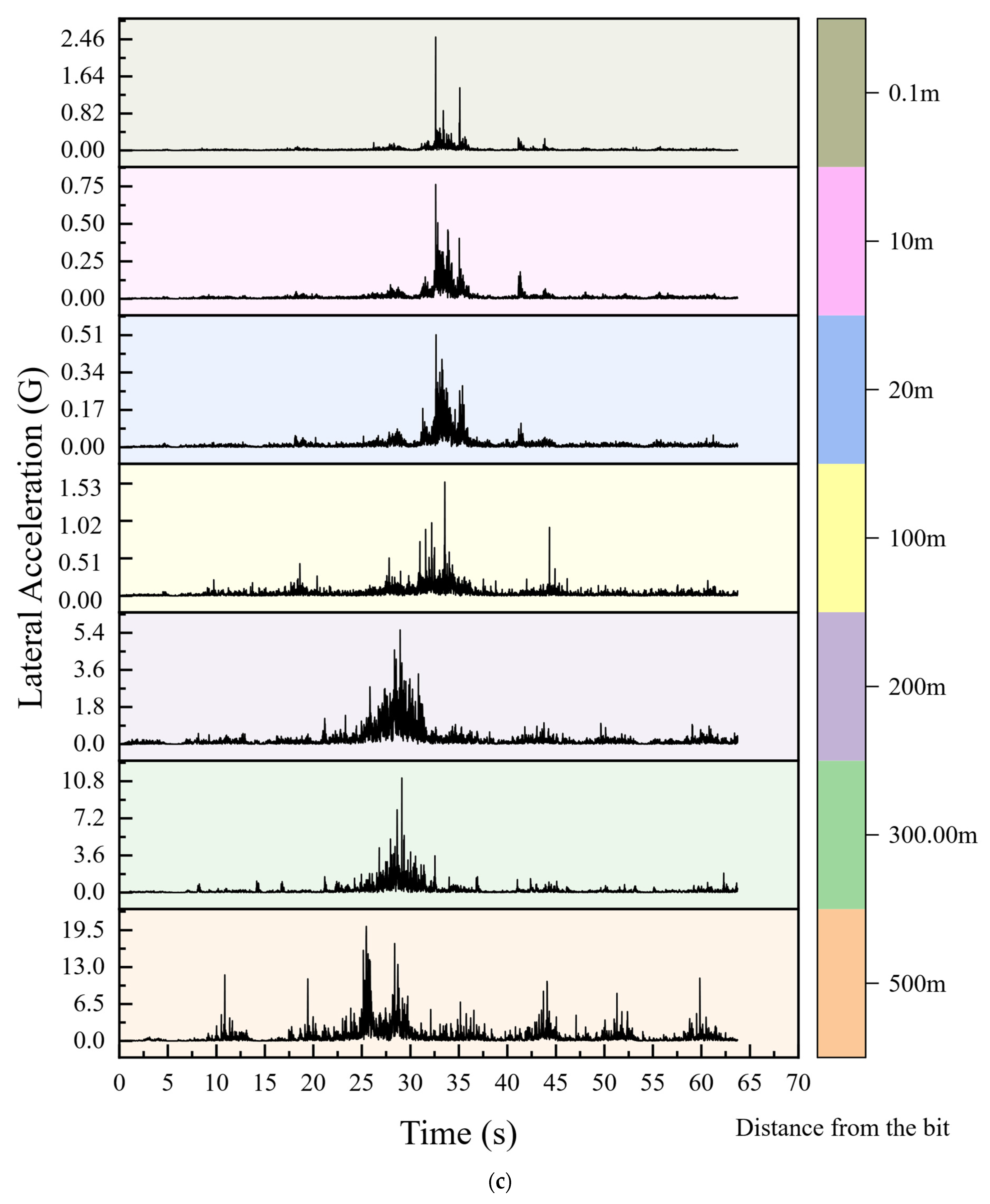
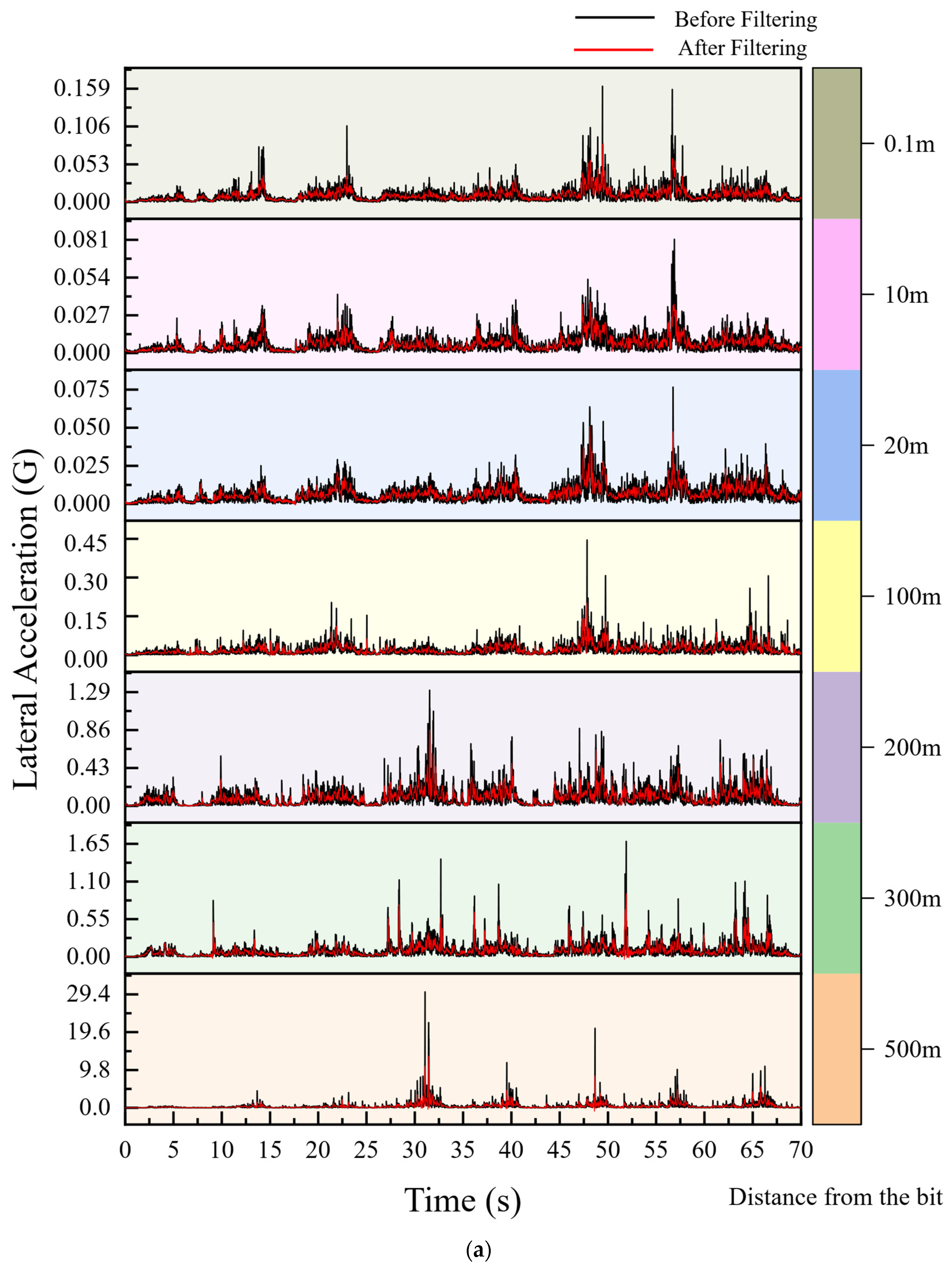
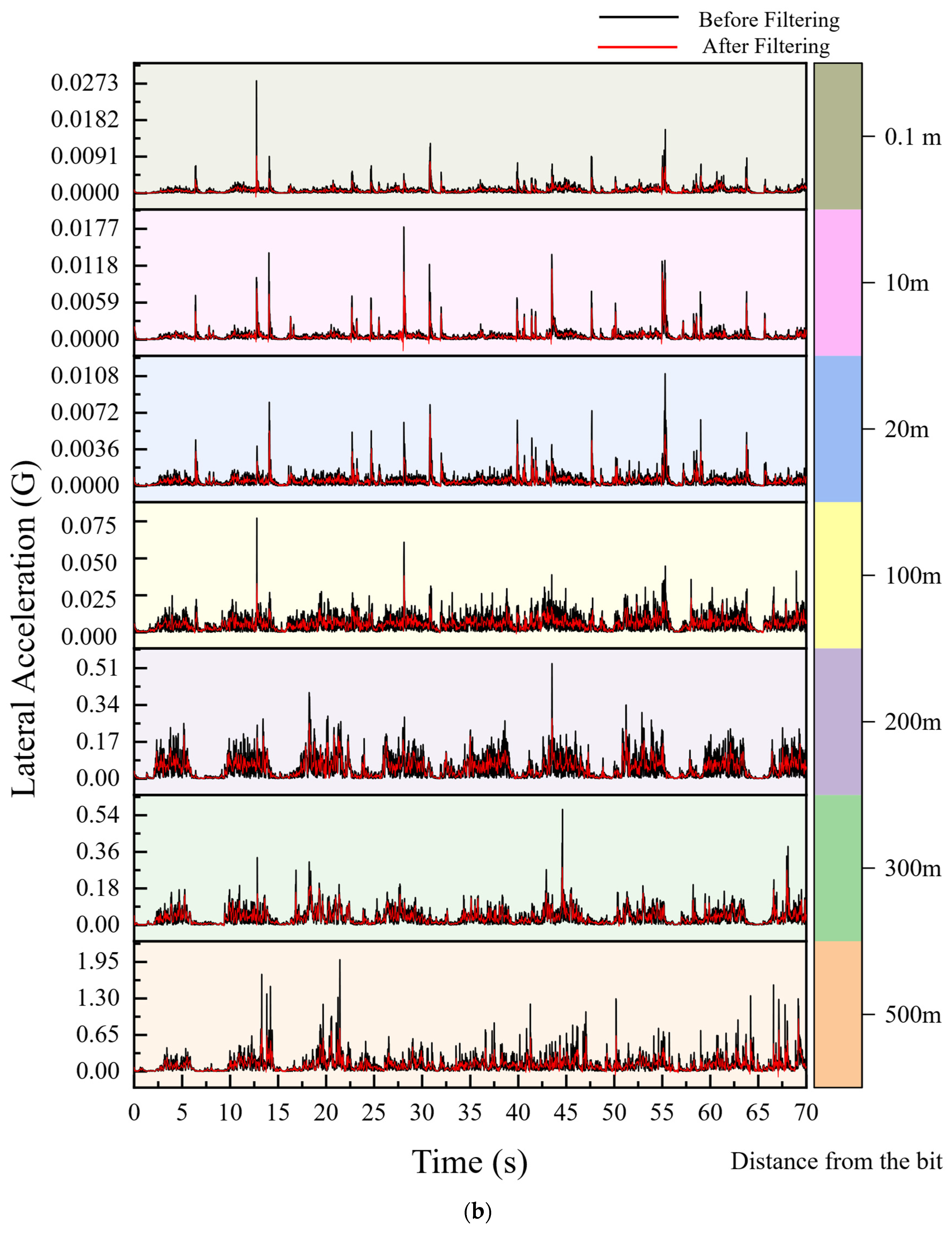
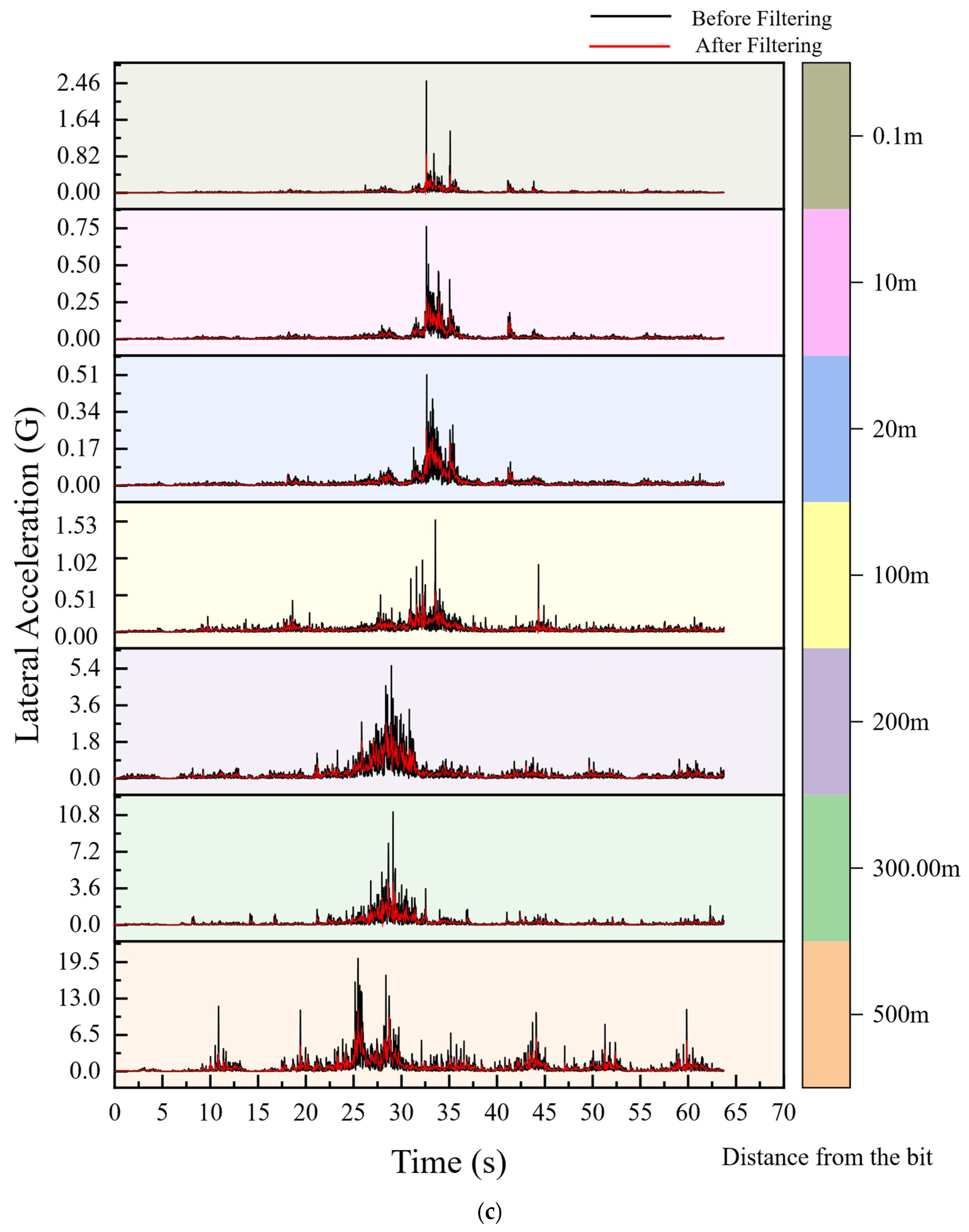
The rate of penetration was kept constant at 3.72 m/h under all three operating conditions. A low-solids, nondispersive, water-based drilling fluid was selected. To further analyze the influence of bottomhole and shallow drill string vibrations and thoroughly examine vibration-wave propagation, seven points were strategically selected upward from the bottom of the well for dynamic analysis, at distances of 0.1, 10, 20, 100, 200, 300, and 500 m from the drill bit. The time histories of lateral acceleration at each point under the three operating conditions are illustrated in Figure 5.

Figure 5. Lateral acceleration under three operating conditions. (a) Lateral acceleration at each point under Working Condition 1; (b) Lateral acceleration at each point under Working Condition 2; (c) Lateral acceleration at each point under Working Condition 3.

Figure 5 shows that drill string vibration consistently propagates upward from the bottom with a delay under the different operating conditions; vibration first appears at the drill bit position. As the vibration energy progressively propagates upward, the upper sections of the drill string subsequently begin to vibrate. The lateral acceleration of the bottomhole node was much higher than that of the other nodes, indicating frequent high-frequency collisions between the drill string and borehole wall. At the same time, whirling amplifies this mechanical response. Furthermore, during drilling, the drill bit penetrates the formation, with most of the energy used to break rock and only a small portion converted into vibration. The vibration amplitudes at different positions along the drill string differ substantially, significantly affecting machine learning accuracy.

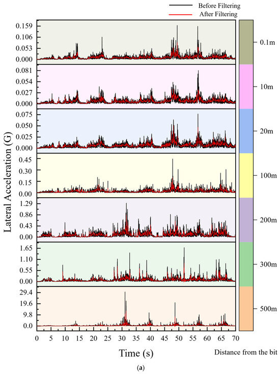
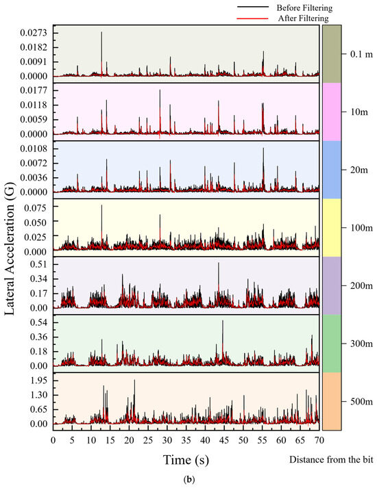
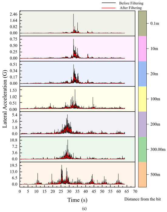
Consequently, points located within 500 m of the drill bit are selected in this study to predict drill string vibration, and Fourier low-pass filtering is used to process the vibration signals, removing large lateral acceleration components while precisely retaining the original vibration waveform. The signals were sampled at approximately 78.125 Hz, corresponding to a mean sampling interval of 0.0128 s and the Nyquist frequency of 39.0625 Hz. A cutoff frequency of 9.76563 Hz was selected for the Fourier low-pass filtering, which is exactly one-eighth of the sampling frequency and corresponds to a normalized cutoff frequency of 0.25 relative to the Nyquist frequency. This cutoff value was determined through comprehensive consideration of three aspects. Firstly, the integer frequency ratio between the cutoff and sampling frequency aligns with the discrete frequency bins of the fast Fourier transform, effectively avoiding spectral leakage and the Gibbs phenomenon during signal reconstruction and ensuring minimal waveform distortion. Secondly, it matches the dominant frequency band of drill string lateral vibration: with the rotary speed ranging from 60 to 150 r/min (1–2.5 Hz), the core components of lateral whirling and wellbore collision responses are concentrated below 10 Hz. Spectrum analysis verifies that over 95% of the effective vibration energy is distributed within the 0–9.76563 Hz band, while higher-frequency components are mainly local collision spikes and numerical discretization noise. Third, retaining low-frequency dominant components while suppressing high-frequency fluctuations helps the subsequent machine learning model capture the intrinsic propagation pattern of vibration, rather than overfitting random high-frequency details. In the frequency domain, Fourier components with absolute frequencies at or below 9.76563 Hz were retained, whereas components above the cutoff were removed; the filtered signals were subsequently reconstructed using the inverse Fourier transform. The same filtering procedure was applied independently to all measurement channels while preserving the original sampling times and record lengths. The signals at each point after filtering are illustrated in Figure 6.

Figure 6. Time domain lateral acceleration under three operating conditions after Fourier low-pass filtering. (a) Changes in lateral acceleration after Fourier low-pass filtering under Working Condition 1; (b) Changes in lateral acceleration after Fourier low-pass filtering under Working Condition 2; (c) Changes in lateral acceleration after Fourier low-pass filtering under Working Condition 3.

Because the numerical lateral acceleration amplitudes of the drill string differ substantially among depths, this study systematically normalizes the data to eliminate the influence of differences in orders of magnitude on the machine learning algorithms. The resulting database is presented in Table 3.

Table 3. Machine learning database of drill string lateral acceleration after filtering.

	500 m	300 m	200 m	100 m	20 m	10 m	0.1 m
Data Quantity	15,918	15,918	15,918	15,918	15,918	15,918	15,918
Maximum Value	13.46431	4.1909	2.74029	0.5623	0.2644	0.28842	0.8780
Minimum Value	−0.94274	−0.1702	−0.3573	−0.0214	−0.000702697	−0.00183	−0.0383
Mean Value	0.4222	0.1134	0.0219	0.04166	0.007048037	0.007319659	0.0104

3. Prediction of Drill String Vibrations

3.1. Principle of XGBoost

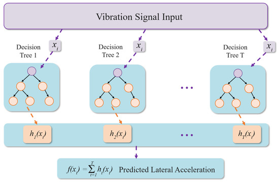
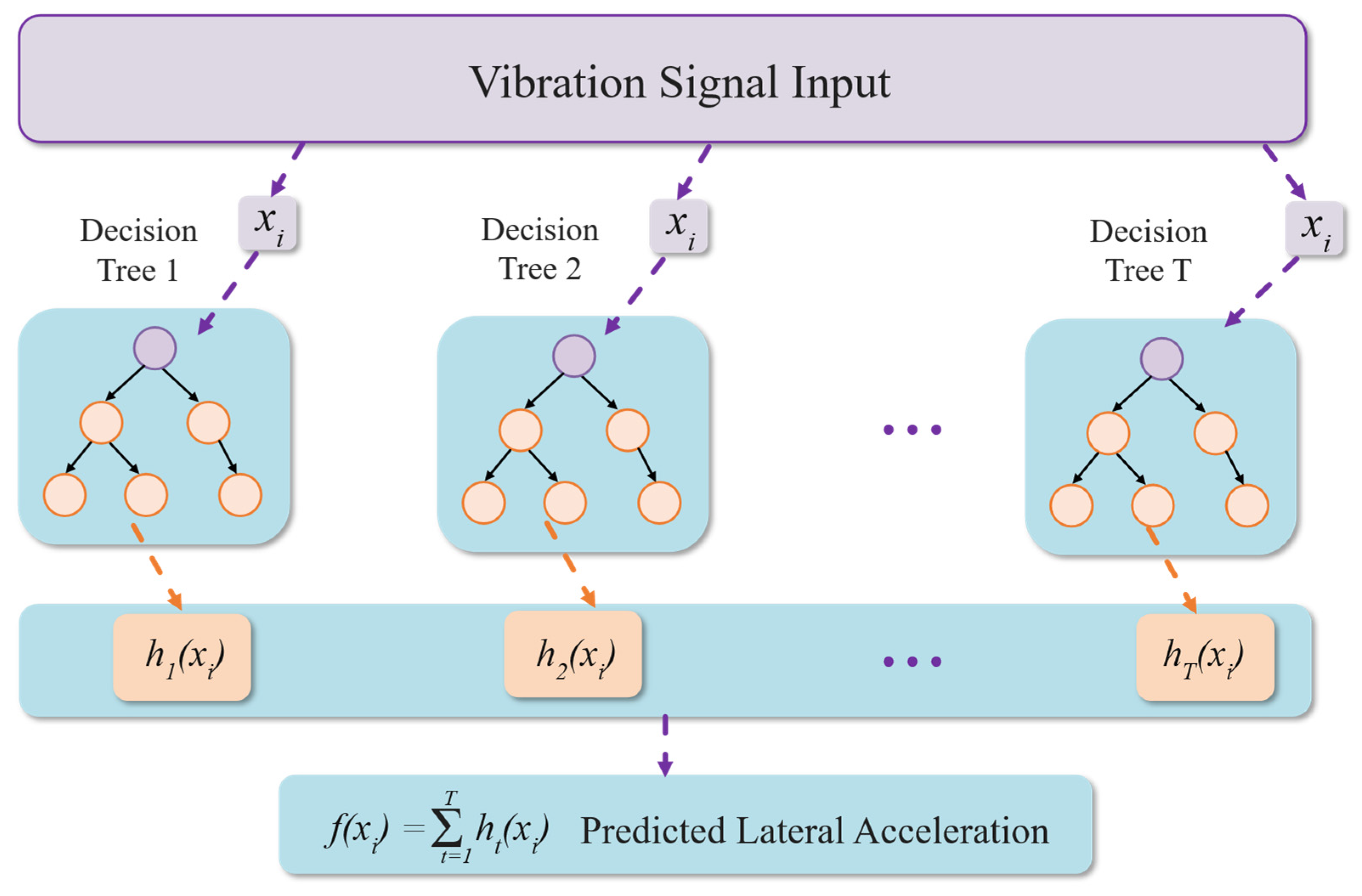
Extreme gradient boosting (XGBoost) integrates multiple weak learners into a single strong learner. The objective of each weak learner is to correct errors generated by all preceding weak learners, thereby reducing the residuals. Its output is the difference between the target value and the predictions accumulated from all preceding components, and the sum of all such outputs yields the final result. Through continuous iteration, XGBoost improves the model’s predictive accuracy. This principle is illustrated graphically in Figure 7.

Figure 7. Schematic of the XGBoost algorithm.

The objective function (Obj) drives the XGBoost algorithm. It constrains model complexity and balances fitting capability and generalizability. The formula for this function is presented in Equation (4).

$${\mathrm{Obj}}^{(t)}=\sum _{i=1}^{n}l(y_i,{\widehat{y}}_i^{(t-1)}+f_t(x_i))+\mathrm{\Omega }(f_t)+constant$$

(4)

where ${\displaystyle \sum _{i=1}^n}l(y_i,{\widehat{y}}_i^{(t-1)}+f_t(x_i))$ denotes the sum of the loss functions of the trees of the preceding (t − 1) number; $\mathsf{\Omega }\left(f_t\right)$ denotes the term of regularization, preventing overfitting of the model; constant denotes the sum of the complexity of the trees of the preceding (t − 1) number. The constant term is independent of $\mathsf{\Omega }\left(f_t\right)$ and does not affect the current optimization.

Hyperopt is used in this study to select hyperparameter combinations for the XGBoost algorithm. Bayesian hyperparameter optimization was performed using the tree-structured Parzen estimator (TPE) algorithm implemented in Hyperopt. Optimization was restricted to the chronologically earlier 70% training block of each operating condition, and candidate parameter configurations were evaluated using fivefold forward-chaining time-series validation. For each validation split, the model was fitted to earlier observations and evaluated on the subsequent validation block, thereby preventing information from future observations or the final 30% test block from entering the optimization procedure. The objective function was the mean validation mean absolute error (MAE) across all condition-specific forward-chaining splits:

$$[\mathcal{L}(\theta )\frac{1}{K}{\displaystyle \sum _{k=1}^K{\mathrm{MAE}}_k}(\theta ),]$$

(5)

where θ denotes the candidate hyperparameter configuration and K is the total number of validation splits.

A total of 200 independent TPE evaluations were conducted to explore the predefined parameter space. The optimization procedure was terminated upon reaching the maximum number of evaluations; no additional early-stopping rule was adopted to avoid premature convergence to local optima and ensure sufficient parameter exploration. To guarantee full reproducibility of the optimization results and subsequent model training, a fixed random seed (seed = 42) was specified for all stochastic operations throughout the workflow, including TPE parameter sampling, time-series data splitting, and XGBoost model initialization. The final parameter combination is presented in Table 4.

Table 4. XGBoost hyperparameter optimization results.

Parameter	Parameter Meaning	Value Range	Optimized Value
max_depth	Decision-tree depth	3–6	3
min_child_weight	Minimum sum of instance weights in a leaf node	1–15	4.0141
gamma	Minimum loss reduction required for a split (minimum gain threshold for node splitting)	0–0.3	2.8305 × 10−5
learning_rate	Learning rate controlling the weight contribution of each tree	0.03–0.15	0.0641
n_estimators	Number of trees	80–200	130
subsample	Subsample ratio: proportion of samples randomly selected to train each tree	0.7–1.0	0.7635
colsample_bytree	Feature-subsample ratio: proportion of features randomly selected for each tree	0.8–1.0	0.9069

3.2. Prediction Results

(1)

Prediction of Lateral Acceleration Using Single-Point Vibration Signals

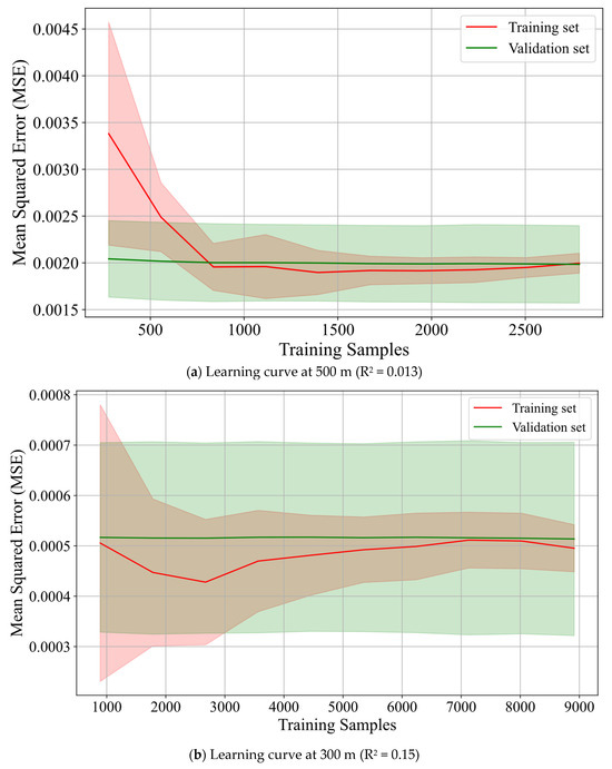
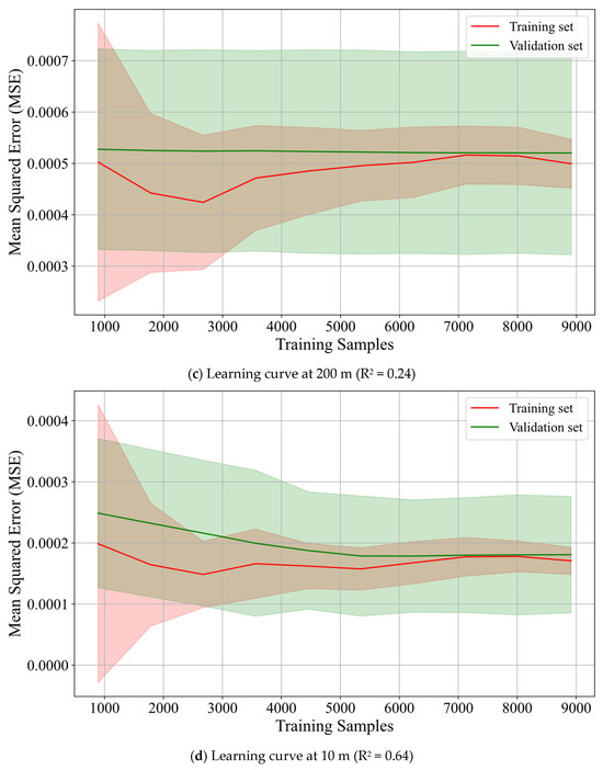
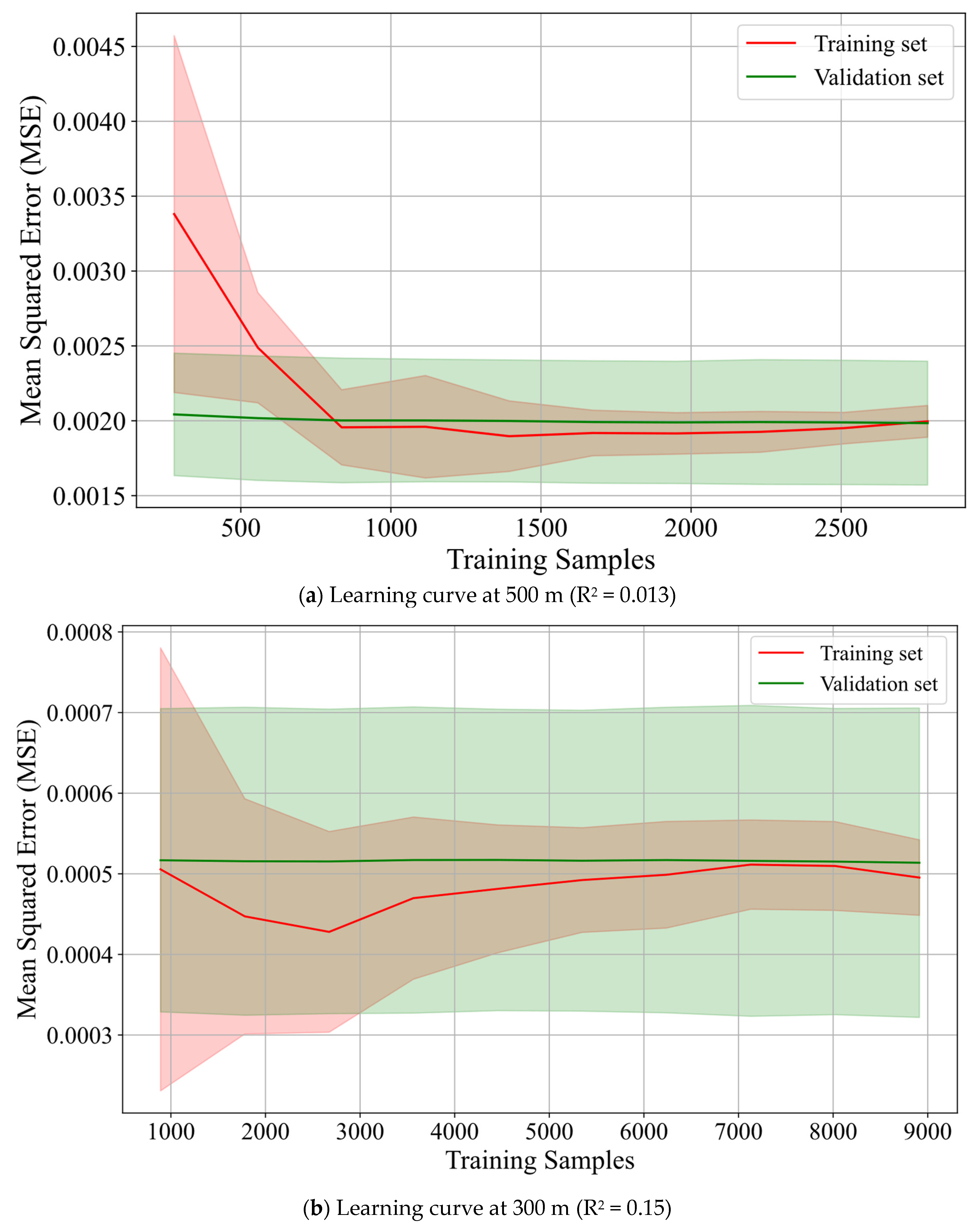
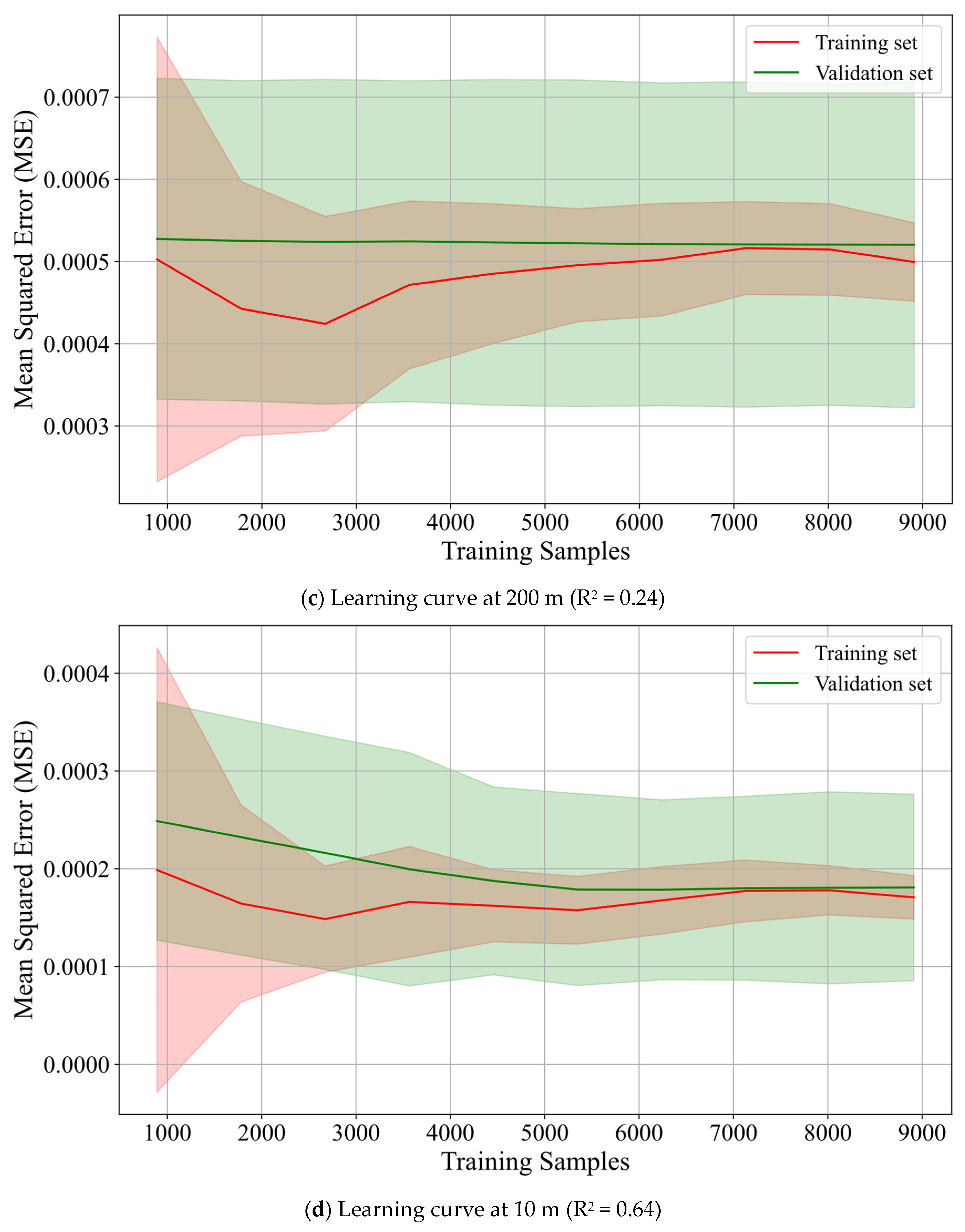
In this study, lateral acceleration signals measured at distances of 500, 300, 200, 100, 20, and 10 m from the drill bit are used as inputs, and bottomhole vibration signals serve as outputs, to establish an XGBoost regression model. For each of the three operating conditions, samples were retained in their original chronological order and divided using a 70/30 time-blocked split. The first 70% of each condition-specific sequence was used for model training and hyperparameter optimization, whereas the remaining 30% was reserved exclusively for independent testing. Hyperparameters were optimized using fivefold forward-chaining time-series validation within the training blocks, ensuring that validation samples always occurred after the corresponding training samples. No random shuffling was applied, and the held-out test blocks were not used during model development. The prediction results are illustrated in Figure 8. It should be noted that “prediction” herein denotes same-time-point prediction with a zero prediction horizon rather than future-time forecasting. Mean squared error (MSE) and the coefficient of determination (R²) serve as indicators of regression model prediction accuracy. A smaller MSE indicates a smaller difference between the model predictions and actual values. The closer R² is to 1, the better the predicted values agree with the actual values. Analyzing the training- and validation-set MSE learning curves as functions of the number of training samples enables evaluation of model performance, degree of fit, and predictive accuracy, thereby guiding model optimization. Figure 8a shows that the XGBoost validation-set learning curve exhibits no large variation and has a relatively low MSE. The model does not learn the association between the two points, as indicated by its coefficient of determination (R² = 0.013). In Figure 8b,c, the model MSE decreases and R² increases relative to Figure 8a, but the validation-set error band remains constant during iteration, indicating insufficient model generalizability, and R² does not exceed 0.7. Although the model learns the association between the two points, it does not fully capture the variation pattern. In Figure 8d, the training- and validation-set error bands converge during iteration, and R² reaches 0.64. The model captures the vibration pattern to some degree, but its predictive reliability remains low. Prediction of bottomhole vibration improves as the selected depth approaches the drill bit. However, single-point prediction performance depends on the monitoring instrument’s installation depth and is not conducive to efficient model prediction.

Figure 8. Learning curves at different prediction depths.

(2)

Prediction of Lateral Acceleration Using Multipoint Vibration Signals

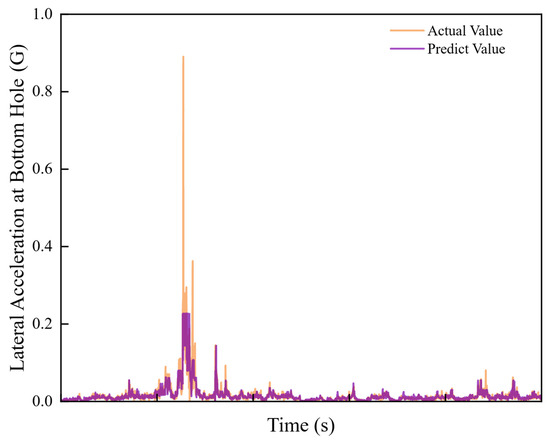
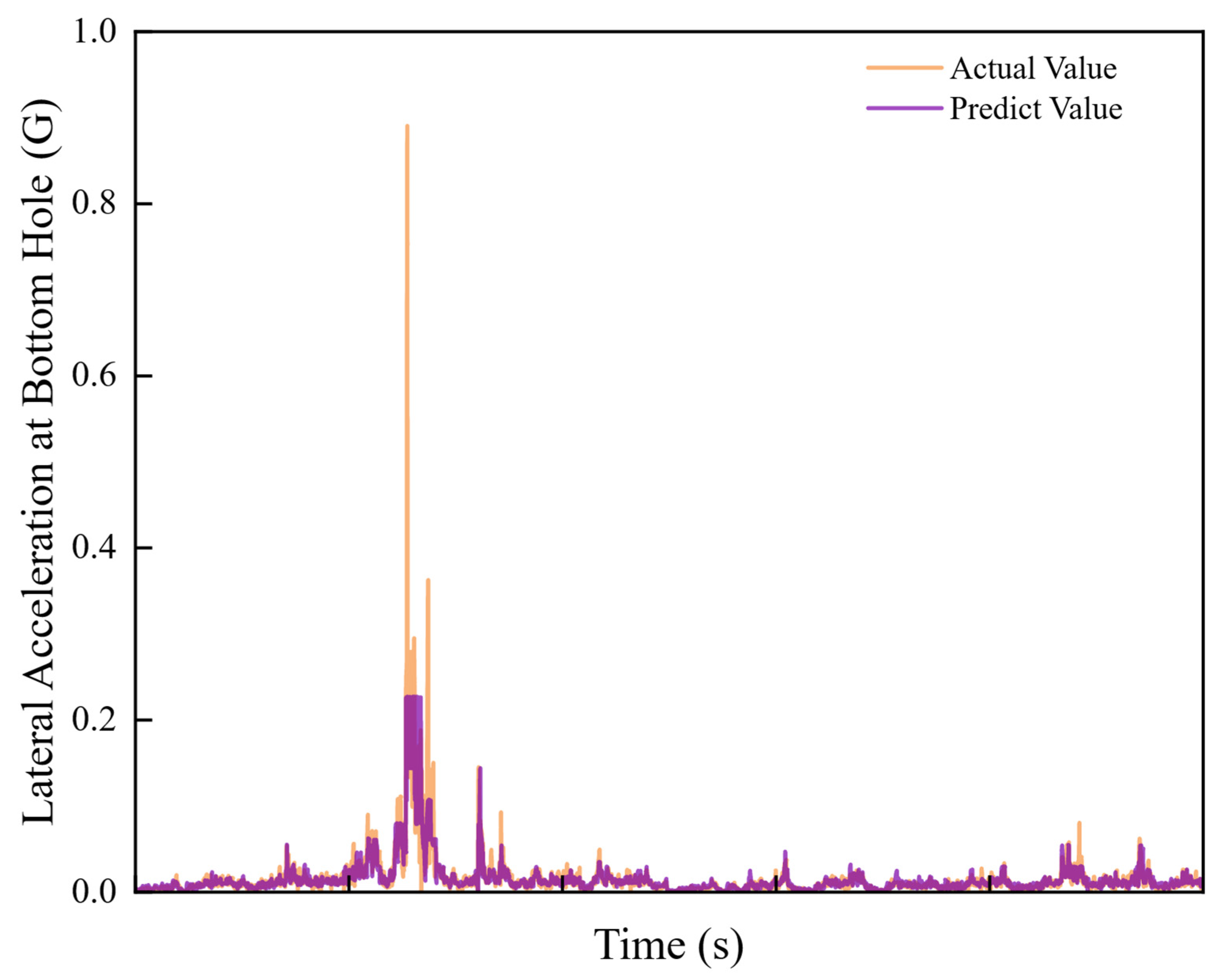
Vibration signals from a single point cannot reflect the vibration pattern of the region in which that point is located. Therefore, this study considers using vibration signals from multiple points to predict bottomhole lateral acceleration. The prediction results are illustrated in Figure 9. Overall, the model successfully captures the general vibration pattern. The coefficient of determination (R²) between the predicted and actual values is 0.7071, indicating that the model captures the vibration waveform. However, the model’s prediction performance is poor at times of large-amplitude vibration, with predictions remaining below the actual values.

Figure 9. Comparison of actual and predicted values.

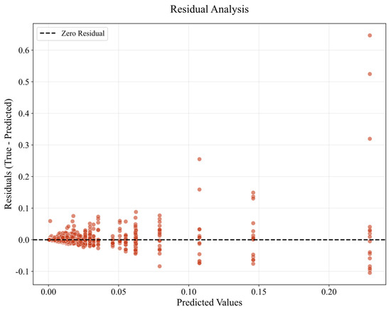
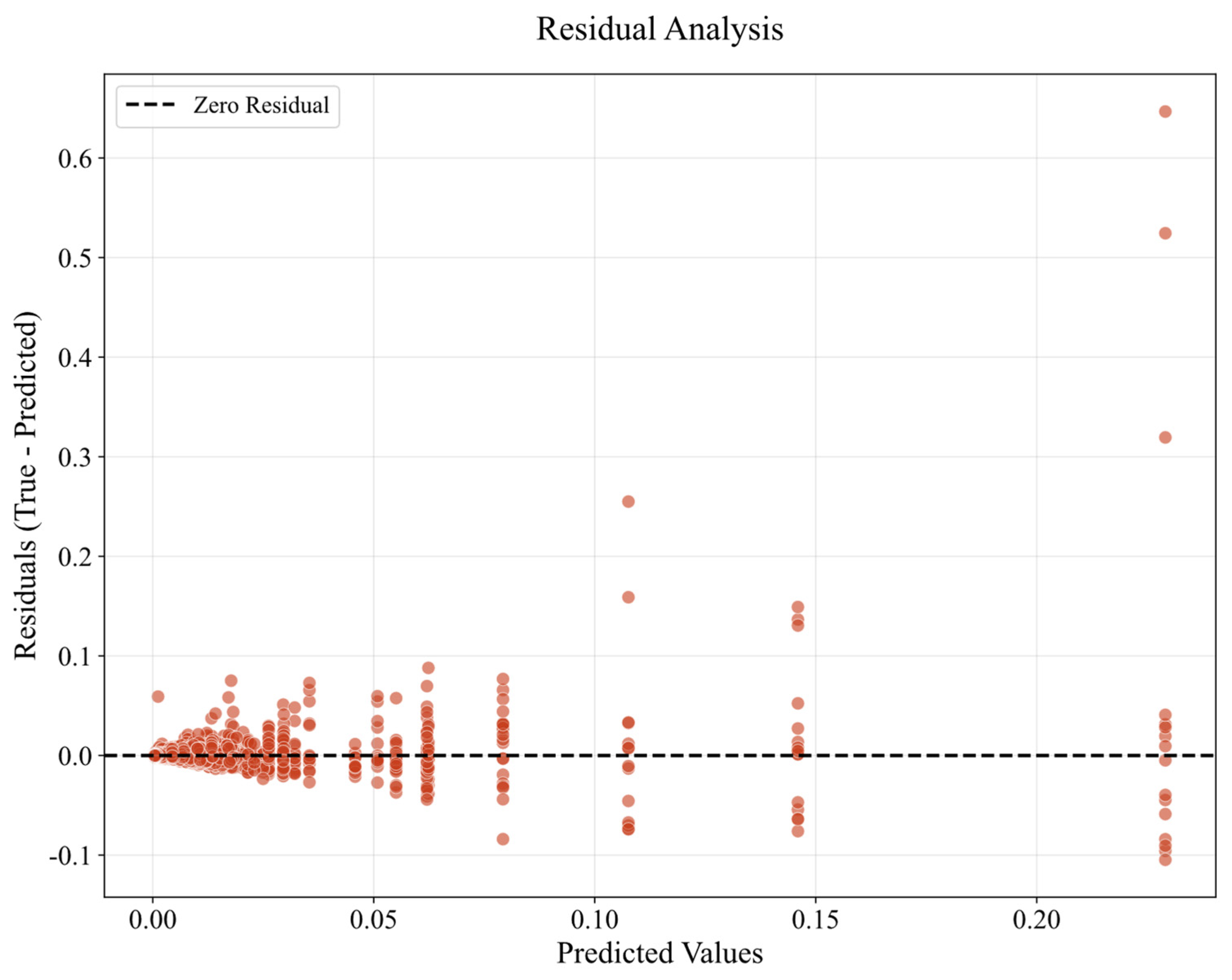
The actual and predicted values are exported for each instance, and their residuals are calculated to analyze the model’s predictive performance for each data group. The results are illustrated in Figure 10. At points where the amplitude predicted by the model is small, the absolute residuals are less than 0.1. This finding reflects accurate model predictions of vibration under normal conditions. At points where the predicted value is larger, the model residual is also larger. As the predicted value increases, the model residual increases, and most residual values are large. This indicates that the model underestimates the actual values. When vibration exceeds a certain threshold, the model reflects only the increasing trend and cannot predict the specific acceleration values.

Figure 10. Residual plot of the prediction model.

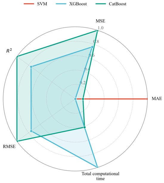
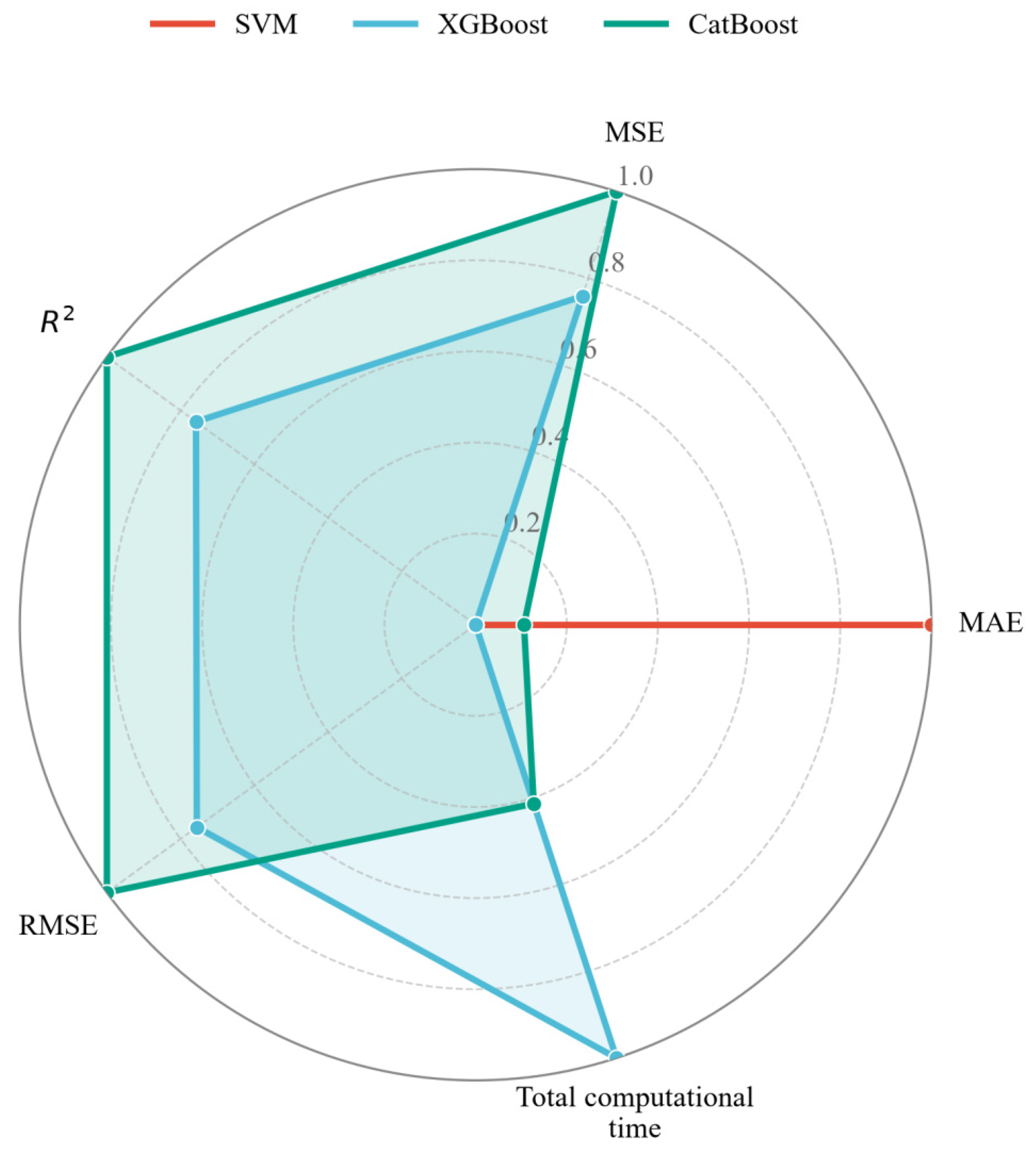
CatBoost and a support vector machine (SVM) are selected as two machine learning algorithms for comparing model accuracy and computational cost in this study. The comparison results are illustrated in Figure 11. To provide an integrated comparison of predictive performance and computational efficiency, MAE, MSE, R², RMSE, and total computational time were normalized and visualized using a radar plot (Figure 11). R² was treated as a benefit criterion, whereas MAE, MSE, RMSE, and computational time were treated as cost criteria; consequently, larger normalized values indicate better performance across all axes. Because the computational times spanned several orders of magnitude, they were logarithmically transformed before min–max normalization. CatBoost achieved the highest overall predictive accuracy, with an R² of 0.7104, an MSE of 2.0704 × 10⁻⁵, and an RMSE of 0.004550. The optimized XGBoost model yielded comparable accuracy, achieving an R² of 0.7071, an MSE of 2.0949 × 10⁻⁵, and an RMSE of 0.004577. Relative to CatBoost, these values corresponded to an R² reduction in only 0.0034 and increases of approximately 1.2% and 0.6% in MSE and RMSE, respectively. SVM produced the lowest MAE (0.002682), although its R² and RMSE were slightly inferior to those of CatBoost. In terms of computational efficiency, XGBoost required only 272.27 s, compared with 3124.70 s for CatBoost and 17,390.87 s for SVM, making it approximately 11.5 and 63.9 times faster, respectively. Overall, CatBoost provided the highest predictive accuracy, while SVM performed best in terms of MAE. However, the optimized XGBoost model achieved the most favorable tradeoff between predictive accuracy and computational cost, retaining accuracy comparable to CatBoost while substantially reducing the total computational burden. Therefore, XGBoost is applicable to drill string vibration prediction.

Figure 11. Comparison of the computational efficiency of three algorithms.

3.3. Physical Limitations of the Machine Learning Models

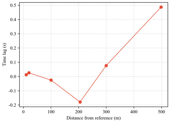
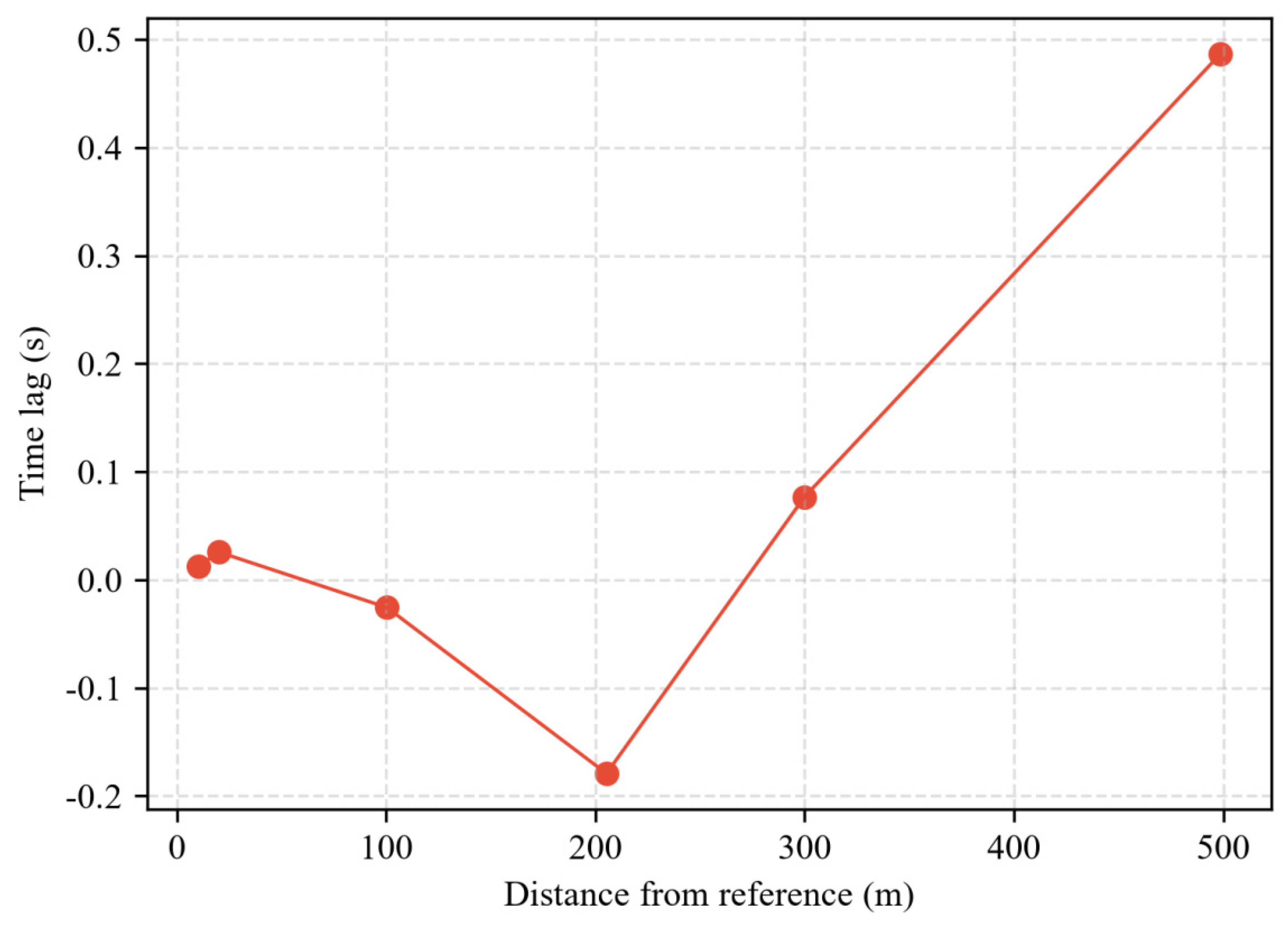
The time domain and frequency domain analyses clarify an important physical limitation of the machine learning models used in this study. The correlation between transmission delay and distance is shown in Figure 12.

Figure 12. Relationship between cross-correlation time lag and distance from the reference location.

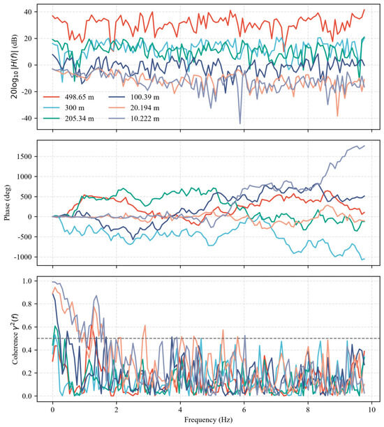
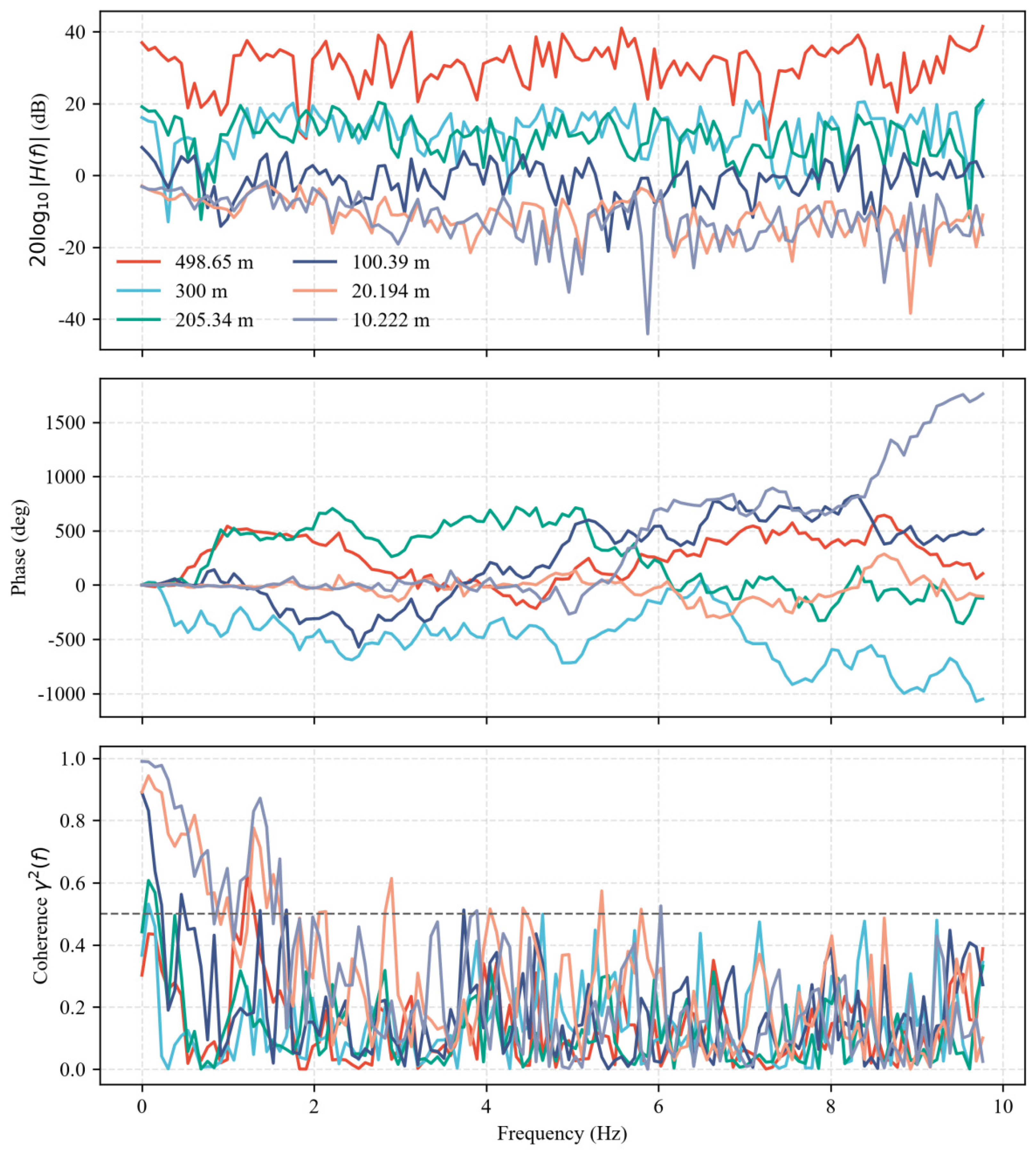
The low-pass-filtered signal at 0.0752 m was used as the reference, and the time lag at each monitoring location was determined from the peak of the normalized cross-correlation function. Positive values indicate that the response lags behind the reference signal, whereas negative values indicate that the selected correlation peak leads the reference signal. The nonmonotonic variation in time lag with distance suggests that vibration transmission cannot be described by a single constant propagation velocity. To further examine the nonmonotonic lag–distance relationship in the frequency domain, the transfer-function magnitude, unwrapped phase, and magnitude-squared coherence were subsequently evaluated at each monitoring location. The frequency-dependent vibration transmission characteristics are shown in Figure 13.

Figure 13. Frequency-dependent vibration transmission characteristics.

Although the agreement between the cross-correlation delay and the group delay estimate at the nearest monitoring location indicates that local vibration propagation can be identified from the simulated signals, the delay–distance relationship becomes nonmonotonic at more distant locations, where the coherence also decreases substantially. This behavior indicates that vibration transmission along the drill string cannot be represented adequately by a single, frequency-independent propagation delay. Instead, the measured responses are consistent with a complex dynamic process involving frequency-dependent attenuation and phase variation, potentially arising from modal superposition, wave reflection, and dispersion.

The low-pass-filtered signal at 0.0752 m was used as the reference input. The H1 transfer-function estimator was calculated as

$$H_1(f)=\frac{S_{x{y}_1}(f)}{S_{x{x}_1}(f)}$$

(6)

where S_xx (f) is the auto-spectral density of the reference signal and S_xy (f) is the cross-spectral density between the reference and response signals. Spectral quantities were estimated using Welch’s method with the Hann window, a segment length of 1024 samples, and 50% overlap. The analysis was restricted to the low-pass-filtered frequency range of 0–9.76563 Hz. The horizontal dashed line denotes the coherence threshold of γ² = 0.5, above which the estimated transfer-function phase and group delay were considered sufficiently reliable for physical interpretation.

The present machine learning models cannot explicitly resolve these propagation mechanisms because they use contemporaneous time domain amplitudes as input features and do not contain variables that directly represent sensor distance, historical time lags, spectral amplitude, phase, coherence, wavenumber, or material and geometric properties. Consequently, the models learn a statistical mapping between simultaneously observed input and output variables rather than the governing space–time relationship of wave propagation. In particular, propagation velocity is defined by the relationship between travel time and distance, while dispersion requires characterization of the frequency-dependent phase or group velocity. Neither quantity is explicitly identifiable from an instantaneous regression mapping without spatial coordinates, lagged observations, or phase-resolved spectral information. Therefore, a high predictive accuracy does not imply that the model has recovered the physical propagation velocity or the underlying dispersion relation.

Accordingly, the predictions should be interpreted as data-driven estimates that are valid primarily for temporally separated samples within the operating conditions, sensor arrangement, and drill string configuration represented in the training data. The current models cannot independently distinguish the contributions of direct wave propagation, structural modes, boundary reflections, attenuation, and dispersion, nor can they be assumed to extrapolate reliably to untested sensor locations, operating conditions, or drill string configurations. Future work should incorporate spatial coordinates, time-lagged inputs, frequency band features, transfer-function magnitude and phase, and coherence-weighted group delay descriptors. Physics-informed or explicitly spatiotemporal architectures may further enable the propagation velocity and frequency-dependent dispersion behavior to be represented more directly.

Based on the aforementioned results, this study presents the recommended installation ranges for downhole vibration-monitoring instruments, as illustrated in Figure 14. The green segment is the recommended zone, in which vibration displacement from a limited number of points predicts bottomhole displacement. The yellow segment is the uncertain zone, in which vibration in this region does not reflect bottomhole vibration. The red segment is the nonrecommended zone, in which the vibration pattern differs greatly from that at the bottomhole and cannot be used to predict the specific value of bottomhole lateral vibration. For the western Sichuan well used in this study, the recommended zone extends from 10 to 300 m from the drill bit; the uncertain zone extends from 300 to 500 m from the drill bit; and the nonrecommended zone extends from 500 m from the drill bit to the wellhead.

Figure 14. Recommended installation ranges for downhole vibration-monitoring instruments.

4. Conclusions

(1)

Lateral acceleration exhibits an upward propagation delay from the bottom, and its magnitude differs by several orders of magnitude between the bottomhole and other positions during drilling. This difference originates from the constraint on radial displacement caused by the bottomhole wellbore diameter approaching the drill bit diameter, together with the energy consumed by rock cutting.

(2)

Predicting bottomhole lateral acceleration using XGBoost and lateral acceleration from deeper layers has limitations. Prediction accuracy decreases as the depth of the points selected as features decreases. The accuracy of predicting drill bit lateral acceleration using single-point lateral acceleration ranges from 1.3% to 64%. Using multiple points from deeper layers to predict bottomhole vibration improves the prediction of bottomhole drill string lateral acceleration to an R² of 0.7071.

(3)

CatBoost, SVM, and XGBoost are compared. In terms of computation time and accuracy, XGBoost has the shortest prediction time and reliable accuracy, making it suitable for predicting bottomhole drill string vibration. Based on the XGBoost bottomhole drill string prediction model, this study proposes recommended installation regions for downhole vibration-monitoring instruments, dividing the drill string into a red nonrecommended zone, a yellow uncertain zone, and a green recommended zone. For the western Sichuan well used in this study, the recommended region extends from 10 to 300 m from the drill bit; the uncertain zone extends from 300 to 500 m from the drill bit; and the nonrecommended zone extends from 500 m from the drill bit to the wellhead.

References

- Li, Q.; Wang, F.; Wu, J.; Li, Q.; Zhang, G. Multivariate coupling model and reservoir characteristics of enhanced geothermal reservoirs. Energies 2026, 19, 3180. [Google Scholar] [CrossRef] [Scilit]
- Li, Q.; Li, Q.; Wu, J.; He, K.; Xia, Y.; Liu, J.; Wang, F.; Cheng, Y. Wellhead stability during development process of hydrate reservoir in the northern South China Sea: Sensitivity analysis. Processes 2025, 13, 1630. [Google Scholar] [CrossRef] [Scilit]
- Li, Q.; You, D.; Li, Q.; Wang, F.; Wang, Y.; Yang, Y. Analysis of sedimentation behavior and influencing factors of solid particles in CO2 fracturing fluid. Processes 2025, 13, 4049. [Google Scholar] [CrossRef] [Scilit]
- Di, Q.F.; Wang, W.C.; Hu, Y.B.; Zhang, X. Study and application of drilling string dynamics. Nat. Gas Ind. 2006, 26, 57–59. [Google Scholar]
- Wang, W.C.; Xu, Z.K.; Zhou, X.; Wang, Z.; Chen, F. Dynamic fatigue failure characteristics and parameter optimization of drill strings in ultra-deep wells. Pet. Drill. Tech. 2024, 52, 118–125. [Google Scholar] [CrossRef]
- Di, Q.F.; You, M.M.; Li, T.X.; Zhou, X.; Yang, H.; Wang, W. Simulation and analysis of dynamic characteristics of drilling string in extra-deep wells. Pet. Drill. Tech. 2024, 52, 108–117. [Google Scholar] [CrossRef]
- Zhu, X.H.; Li, K.; Li, W.Z.; He, M.; She, Z.; Tan, B. Drill string mechanical behaviors of large-size borehole in the upper section of a 10,000 m deep well. Nat. Gas Ind. 2024, 44, 49–57. [Google Scholar] [CrossRef]
- Gao, G.H.; Qiu, X.Q.; Dong, H.; Xu, J.; Ren, H. Analysis on the torsional vibration of ultra-deep water drill string. Ind. Heat. 2016, 45, 13–16. [Google Scholar]
- Zhao, Z.B.; Qiu, X.Q.; Xu, J.L. Finite element analysis of modal vibrations of drill strings in deep-sea natural gas hydrate coring/drilling. Nat. Gas Ind. 2011, 31, 73–76. [Google Scholar]
- Lubinski, A. A study of the buckling of rotary drilling string. Drill. Prod. Pract. 1950, 34, 178–214. [Google Scholar]
- Finnie, I.; Bailey, J.J. An experimental study of drill-string vibration. J. Eng. Ind. 1960, 82, 129–135. [Google Scholar] [CrossRef] [Scilit]
- Dareing, D.W.; Livesay, B.J. Longitudinal and angular drill-string vibrations with damping. J. Eng. Ind. 1968, 90, 671–679. [Google Scholar] [CrossRef] [Scilit]
- Millheim, K.K.; Jordan, S.; Ritter, C.J. Bottom-hole assembly analysis using the finite-element method. J. Pet. Technol. 1978, 30, 265–274. [Google Scholar] [CrossRef] [Scilit]
- Zhang, Y.L.; Xiao, Z.Y.; Duanmu, G. Study of the principle of motion for the rotating drill string. Oil Field Equip. 1988, 2, 1–7. [Google Scholar]
- Clayer, F.; Vandiver, J.K.; Lee, H.Y. The effect of surface and downhole boundary conditions on the vibration of drillstrings. In Proceedings of the SPE Annual Technical Conference and Exhibition, New Orleans, LA, USA, 23–26 September 1990. Paper SPE-20447-MS. [Google Scholar] [CrossRef]
- Liu, Y.Q. A study of tridimensional double nonlinear dynamics of drillingstring in annulus. Chin. J. Theor. Appl. Mech. 1998, 30, 96–103. [Google Scholar]
- Remmert, S.M.; Witt, J.W.; Dupriest, F.E. Implementation of ROP management process in Qatar North Field. In Proceedings of the SPE/IADC Drilling Conference, Amsterdam, The Netherlands, 20–22 February 2007; Society of Petroleum Engineers: Richardson, TX, USA, 2007. [Google Scholar] [CrossRef]
- Di, Q.F.; Luo, D.F.; Zhou, X.; Wang, W.; Chen, F. Analysis of dynamic characteristics of bottom hole assembly under transverse active deviation control force. Acta Pet. Sin. 2023, 44, 1552–1561+1573. [Google Scholar] [CrossRef]
- Fan, Z.; Zhang, C.; Wang, D.; Li, S.; Zhao, J.; Wu, Z. Thermoporoelastic response of a semi-permeable wellbore subjected to convective cooling and non-hydrostatic in situ stresses. Int. J. Numer. Anal. Methods Geomech. 2023, 47, 2116–2135. [Google Scholar] [CrossRef] [Scilit]
- Li, Z.; Zhang, C.; Fan, Z.; Qiu, Y.; Li, X.; Zhao, L. Analytical solutions for transient response of a semi-permeable wellbore subjected to non-hydrostatic in situ stresses and convective boundary conditions within a transversely isotropic thermoporoelastic medium. Geomech. Energy Environ. 2026, 45, 100801. [Google Scholar] [CrossRef] [Scilit]
- Zhang, Z.H. Application of the wavelet neural network in diagnosis of drilling accidents. Oil-Gas Field Surf. Eng. 2013, 32, 6–7. [Google Scholar]
- Zhu, X.H.; Jia, Y.J. Research progress and applications of drill string dynamics. In Theory of Mechanical Dynamics and Applications; Chinese Society for Vibration Engineering, Ed.; School of Mechanical and Electrical Engineering, Southwest Petroleum University: Chengdu, China, 2011; p. 11. [Google Scholar]
- Yi, P.; Liu, Y.C.; Guo, X.; Li, J. Optimal design of drilling parameters based on an improved adaptive genetic algorithm. China Pet. Mach. 2010, 38, 30–33+73. [Google Scholar]
- Saadeldin, R.; Gamal, H.; Elkatatny, S.; Abdulraheem, A. Intelligent model for predicting downhole vibrations using surface drilling data during horizontal drilling. J. Energy Resour. Technol. 2022, 144, 083002. [Google Scholar] [CrossRef] [Scilit]
- Huang, H.L.; Wang, B.; Li, J.; Yang, H.W.; Gao, R.Y.; Zhang, G.; Luo, M.; Li, W.T. Study on stick-slip early warning model based on LSTM. In Proceedings of the 56th U.S. Rock Mechanics/Geomechanics Symposium, Santa Fe, NM, USA, 26–29 June 2022. [Google Scholar]
- Zhang, F.F.; Cui, Y.H.; Yu, C.; Zhang, T.; Chen, J. Recent developments and future trends of drilling status recognition technology based on machine learning. J. Yangtze Univ. Nat. Sci. Ed. 2023, 20, 53–65+143. [Google Scholar] [CrossRef]
- Chen, J.; Yang, L.; Huang, Q.; Zhang, W.; Qiao, J.; Zhang, X.; Jiang, D. Dynamic analysis of drill string vibration enhanced by neural network based models. Geoenergy Sci. Eng. 2025, 246, 213618. [Google Scholar] [CrossRef] [Scilit]
- Song, J.; Liu, S.; Jiang, S.; He, Y.; Wu, Y.; Zhu, H. Simulation and analysis of drill string vibration in natural gas hydrates drilling. J. Vib. Eng. Technol. 2025, 13, 327. [Google Scholar] [CrossRef] [Scilit]
- Zhu, L.P.; Wang, X.Y.; Yan, Y.C. Application of formation-pressure monitoring while drilling in western Sichuan. Nat. Gas Technol. 2009, 3, 37–39. (In Chinese) [Google Scholar]
Disclaimer/Publisher’s Note: The statements, opinions and data contained in all publications are solely those of the individual author(s) and contributor(s) and not of MDPI and/or the editor(s). MDPI and/or the editor(s) disclaim responsibility for any injury to people or property resulting from any ideas, methods, instructions or products referred to in the content. |
© 2026 by the authors. Licensee MDPI, Basel, Switzerland. This article is an open access article distributed under the terms and conditions of the Creative Commons Attribution (CC BY) license.