Hybrid Deterministic, Regression and Machine Learning Framework for Endpoint Temperature Prediction and Scrap Charge Optimization in BOF Steelmaking

Abstract

Scrap charge selection has a significant influence on the thermal balance of the basic oxygen furnace (BOF) process and consequently on the final melt temperature. This paper presents a hybrid deterministic, regression, and machine learning framework for endpoint temperature prediction and steel scrap charge optimization in BOF steelmaking. The proposed methodology combines an existing deterministic BOF simulation model with regression analysis, machine learning surrogate models, and constrained nonlinear optimization. The dataset was constructed from operational records of 180 industrial BOF heats. The masses of seven scrap categories and the target endpoint temperature were obtained from these operational records, whereas the endpoint temperature used as the output for training the machine learning surrogate models was generated by the existing deterministic BOF process model. Three machine learning approaches, namely Support Vector Regression (SVR), Random Forest Regression (RF), and Gaussian Process Regression (GPR), were implemented and evaluated for endpoint temperature prediction using the masses of seven scrap categories and the target endpoint temperature as model inputs. Among the investigated surrogate models, Gaussian Process Regression achieved the best approximation performance, with a test MAE of 10.47 °C, RMSE of 16.38 °C, and $R^2$ = 0.870, and was subsequently used in the optimization framework. In addition, the deterministic BOF simulation model was incorporated into a model-based optimization procedure using the same optimization objective. Both approaches were formulated as constrained optimization problems minimizing the deviation between the predicted and target endpoint temperatures while satisfying the total scrap mass constraint. The proposed framework provides a model-based approach to temperature-oriented scrap charge planning using either a machine learning surrogate model or a detailed deterministic process model.

1. Introduction

The Basic Oxygen Furnace (BOF), also known as the LD converter process, is one of the most widely used technologies for primary steelmaking worldwide. The thermal and chemical behavior of the BOF process strongly influences steel quality, production efficiency, energy consumption, refractory lifetime, and overall operational costs. One of the key technological objectives is achieving the desired endpoint temperature of molten steel at the end of the oxygen blowing process [1,2,3,4,5].

Predicting the endpoint temperature is essential for a stable and efficient BOF process. Excessively high temperatures may increase refractory wear, oxidation losses, and energy consumption, whereas insufficient temperatures can require additional reheating operations or corrective process interventions, leading to increased production costs and reduced productivity. Consequently, endpoint temperature prediction has become an important research topic in modern intelligent steelmaking systems [2,3,4,5,6,7,8,9,10,11,12].

The converter’s thermal state at the endpoint is affected by many process variables, including the chemical composition and temperature of hot metal, oxygen consumption, slag-forming additions, and, in particular, the amount and composition of scrap charged into the converter. Steel scrap materials represent an important cooling component in the process and significantly influence the thermal balance of the heat. However, different scrap categories exhibit different thermal and metallurgical behavior due to variations in chemical composition, density, contamination, geometry, and heat absorption capability [1,13,14,15,16,17,18,19,20,21].

In industrial practice, the determination of suitable scrap composition is typically based on empirical knowledge, simplified regression models, static thermal calculations, or operator experience. Nevertheless, the BOF process is characterized by strong nonlinearities and complex interactions among technological variables, which limit the prediction capability of conventional linear approaches. Therefore, advanced data-driven methods and machine learning techniques have attracted increasing attention in recent years [3,4,5,10,11,12,22].

Machine learning methods provide an effective way to approximate nonlinear relationships directly from historical process data without explicitly formulating the underlying physical equations. Various machine learning approaches have been investigated for BOF endpoint prediction and related steelmaking applications [3,4,5,6,7,8,9,10,11,12,22,23,24,25].

In addition to process prediction, machine learning methods can also be utilized for optimization-oriented applications in steelmaking. Once trained, ML models can serve as fast surrogate models approximating the behavior of more computationally demanding empirical, thermodynamic, or metallurgical models [26,27]. Such surrogate models can be attractive for optimization tasks because they allow repeated evaluation of the modeled process response at relatively low computational cost. Consequently, they enable rapid evaluation of multiple process scenarios and can be integrated into intelligent decision-support systems for industrial operation.

In BOF steelmaking, optimizing the composition of steel scrap is an important technological and economic task. Different scrap categories influence the thermal balance of the process in different ways, and an unsuitable scrap distribution may lead to significant deviations from the desired endpoint temperature. Industrial operators therefore face the problem of determining suitable scrap proportions while simultaneously satisfying technological constraints such as total allowable scrap mass and operational limitations [26,27,28,29,30,31,32,33].

The optimization of scrap charge composition is a challenging problem because the relationship between scrap distribution and endpoint temperature is strongly nonlinear. Moreover, practical optimization must consider multiple constraints and interactions among individual process variables [26,27,28,30,31,32]. Traditional optimization approaches based solely on empirical rules or simplified linear models may therefore provide limited performance and poor generalization capability. Moreover, repeated evaluation of detailed deterministic BOF models during optimization may become computationally demanding, which motivates the use of surrogate models.

A promising solution is to combine machine learning surrogate models with nonlinear constrained optimization algorithms. In such an approach, the trained ML model predicts the endpoint temperature for a given scrap composition, while an optimization algorithm iteratively searches for the scrap distribution minimizing the temperature prediction error under technological constraints.

This work focuses on the development and comparison of machine learning surrogate models for prediction of the BOF endpoint temperature based on scrap composition and target process temperature. The input variables investigated include the masses of seven scrap categories, along with the target endpoint temperature. The output variable corresponds to the endpoint temperature generated by the existing deterministic BOF process model.

Three machine learning approaches were investigated and compared:

• Support Vector Regression (SVR);
• Random Forest Regression (RF);
• Gaussian Process Regression (GPR).

The surrogate models were trained and evaluated using a dataset constructed from operational inputs from 180 industrial BOF heats and endpoint temperatures generated by the deterministic BOF process model. The primary objective was to identify the machine learning approach with the highest prediction accuracy and the best generalization capability. Subsequently, the best-performing model was integrated into an optimization framework for the optimization of scrap mass ($x_i$) under the technological mass-balance condition (1).

$${\sum }_{i=1}^7{x}_i=\mathrm{28,000}$$

(1)

The proposed optimization framework enables an iterative search for scrap distributions that minimize the deviation between the predicted and required endpoint temperatures. The proposed methodology combines deterministic process modeling, regression modeling, machine learning surrogate models, and nonlinear constrained optimization within a unified framework for BOF endpoint temperature prediction and scrap charge optimization.

The main contributions of this work can be summarized as follows:

• development of data-driven ML surrogate models for BOF endpoint temperature prediction;
• comparison of several machine learning methods;
• evaluation of surrogate-model approximation performance using industrial operating inputs and deterministic-model-generated endpoint temperatures;
• development and implementation of a constrained optimization framework for scrap charge optimization;
• demonstration of the feasibility of combining machine learning and nonlinear optimization for BOF process support;
• implementation and comparison of two optimization strategies: constrained optimization using a machine learning surrogate model and optimization using the original deterministic BOF model.

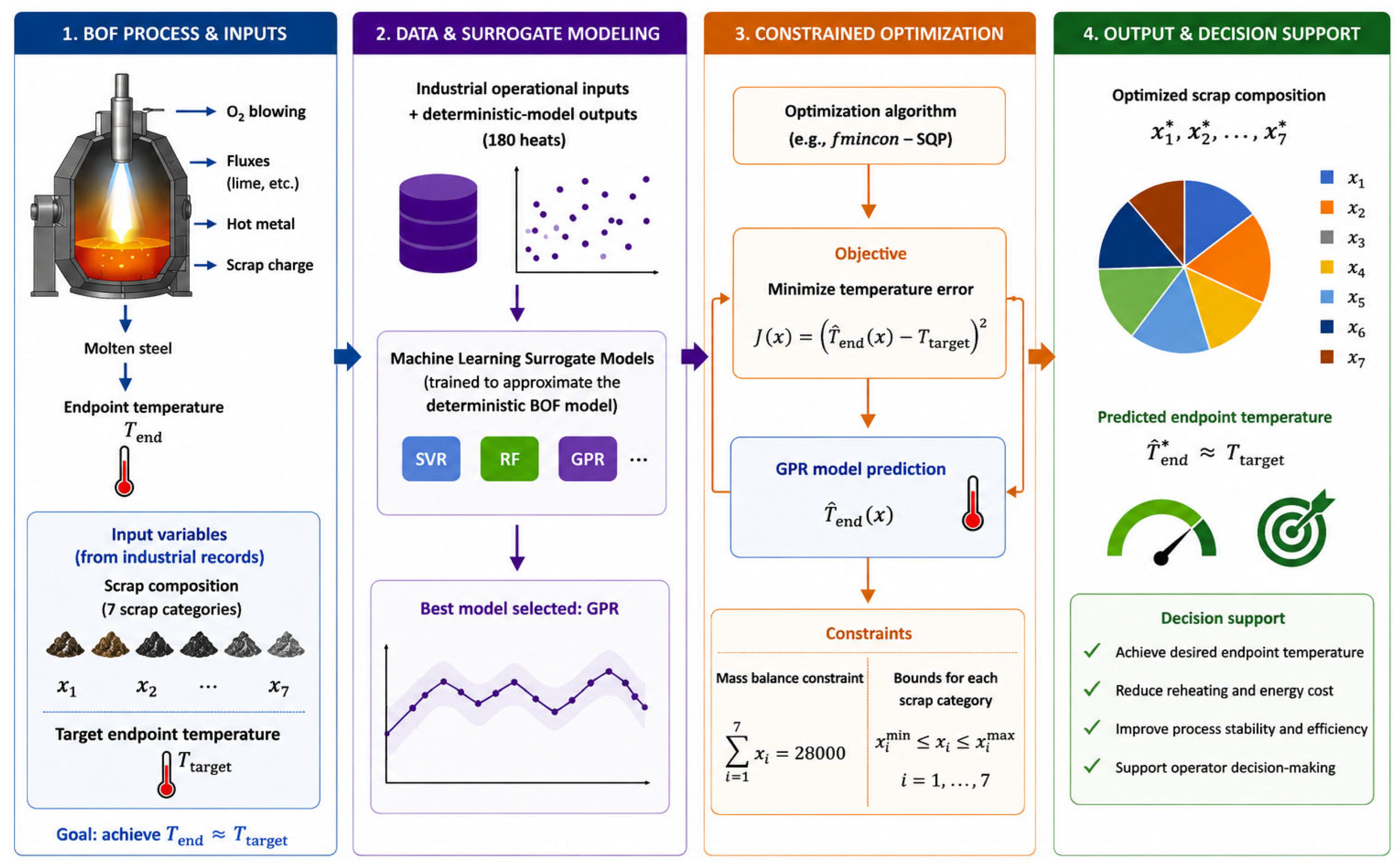
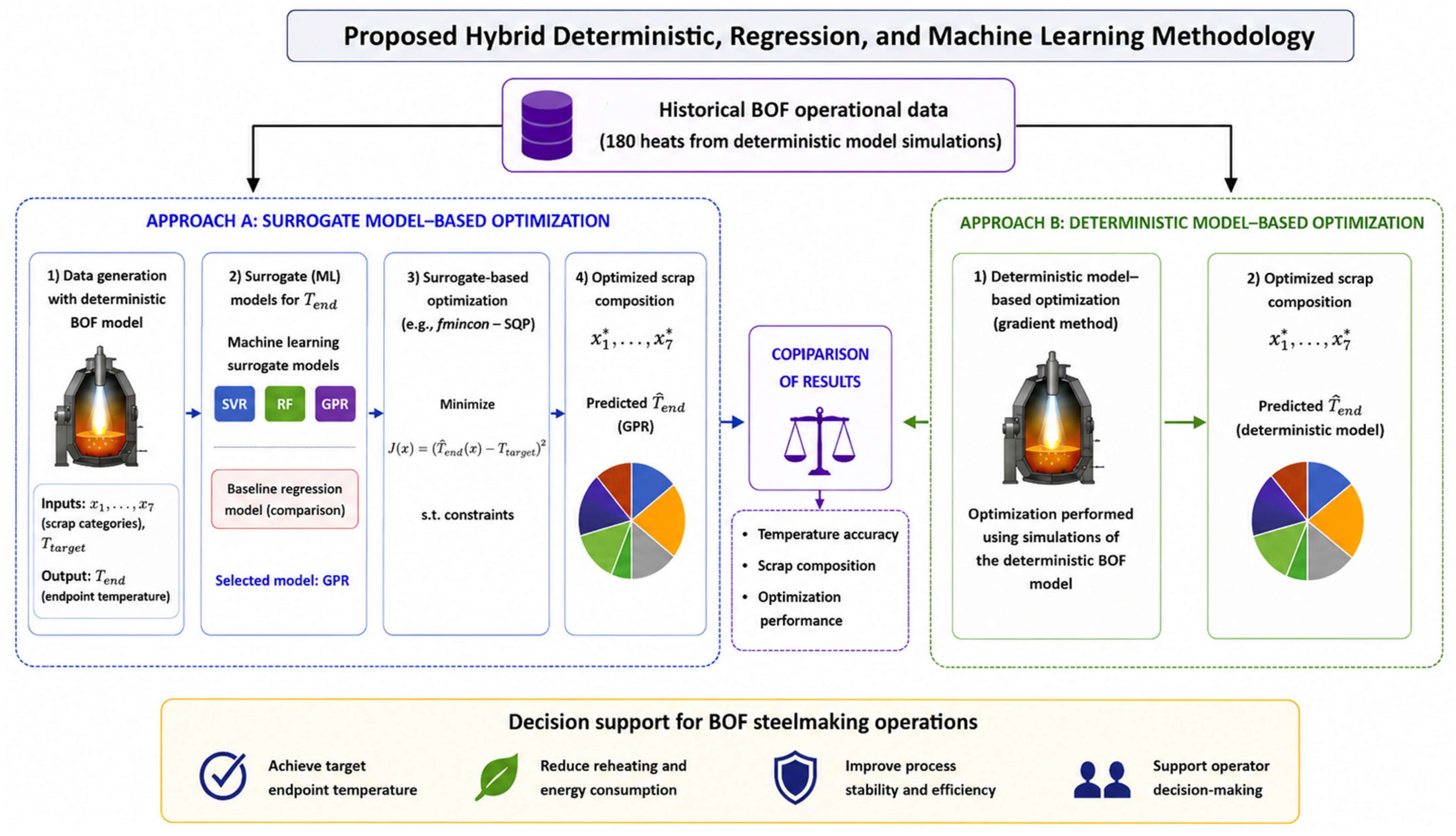
Figure 1 presents a conceptual overview of the proposed intelligent BOF steelmaking framework. The figure illustrates the interaction between the BOF converter process, scrap charge composition, machine learning-based surrogate modeling, and constrained optimization. Industrial operational inputs together with endpoint temperatures generated by the deterministic BOF model are utilized to train the machine learning surrogate models. Subsequently, nonlinear optimization is employed to determine suitable scrap charge distributions satisfying technological constraints while minimizing the endpoint temperature deviation. The proposed framework combines metallurgical process knowledge, machine learning, and optimization-oriented decision support for modern intelligent steelmaking applications.

Figure 1 summarizes the relationships among the individual components of the proposed methodology and illustrates the overall workflow adopted in this study.

The prediction and optimization of endpoint parameters in basic oxygen furnace (BOF) steelmaking have been investigated for several decades because they directly influence steel quality, productivity, energy consumption, refractory wear, and production costs. Endpoint temperature and carbon content are especially important because they determine whether the heat can proceed to secondary metallurgy without additional corrective operations. Inaccurate endpoint control may require reblowing, coolant additions, reheating, or other interventions, which reduce process stability and increase costs.

From a metallurgical viewpoint, scrap charging is one of the key factors affecting the thermal state of the BOF process. Scrap acts as a cooling material, and its melting behavior is coupled with heat transfer, carbon transfer, slag formation, and decarburization kinetics. Early theoretical studies by Asai and Muchi showed that scrap melting significantly affects the temperature trajectory, carbon concentration, and endpoint conditions of the LD converter process [13,14,15]. These works demonstrated that scrap cannot be treated only as a static charge component because its amount and melting rate influence the dynamic thermal and chemical behavior of the converter.

The importance of thermally balanced charge additions was also emphasized in early endpoint temperature control studies. Slatosky [1] formulated thermochemical equations for calculating balanced amounts of scrap, lime, and hot metal in LD steelmaking. Such approaches formed the basis of classical heat-balance endpoint control. Later studies further confirmed that scrap melting depends not only on total scrap mass but also on physical and chemical scrap properties. For example, Kruskopf [16] analyzed scrap melting in a steel converter and showed that heat transfer and carbon mass transfer between the melt and scrap strongly influence melting behavior. More recent works have also studied the effects of scrap size, particle surface, bath temperature, and carburization on melting rate [17,18,19,20,21]. These findings support the need for models that can capture the nonlinear influence of scrap charge composition on endpoint temperature.

Traditional BOF endpoint models are usually based on static heat and material balances, empirical equations, regression models, or operator experience. These models are attractive because they are interpretable and can be connected with metallurgical knowledge. However, the BOF process is highly nonlinear, time-varying, and affected by uncertainties in raw material quality, hot metal composition, scrap properties, oxygen blowing, flux additions, and measurement availability. Therefore, purely deterministic or linear regression-based models may provide limited accuracy under changing industrial conditions.

Several studies have therefore applied data-driven and machine learning methods to BOF endpoint temperature prediction. Neural-network-based approaches were among the first widely used methods. Cai et al. [2] combined DBSCAN-based data preprocessing with an RBF neural network for BOF endpoint temperature prediction. Dong and Dong [6] developed an RBF neural-network model for converter endpoint temperature and carbon prediction using process variables including molten iron, scrap iron, oxygen blowing, and flux additions. Qu et al. [7] proposed an endpoint control strategy using RBF and BP neural networks, where predicted endpoint temperature and carbon content were used to calculate corrective coolant and oxygen additions during reblowing. In the study by Fang et al. [8], through data mining and correlation analysis of the main equipment and processes involved in steel transfer, a network algorithm was optimized to solve the problems of standard back propagation (BP) networks, and a steel temperature forecasting model based on improved back propagation (BP) neural networks was established for basic oxygen furnace (BOF) steelmaking, ladle furnace (LF) refining, and Ruhrstahl–Heraeus (RH) refining.

Support-vector-based methods have also been applied to converter endpoint temperature prediction. Wei et al. [9] proposed an improved least-squares support vector machine optimized by particle swarm optimization for BOF end-temperature prediction. Duan et al. [3] developed a Fireworks Algorithm-optimized Twin Support Vector Regression model for simultaneous endpoint temperature and carbon prediction. These studies showed that kernel-based regression models can provide good nonlinear approximation capability for BOF process data, especially when suitable hyperparameter optimization is applied.

More recent BOF endpoint temperature prediction studies have focused on ensemble learning, feature selection, deep learning, and soft-sensor modeling. Jo et al. [4] compared several machine learning methods for endpoint temperature prediction in LD converters, including linear regression, support vector regression, Random Forest, XGBoost, LightGBM, CatBoost, and a Mixture-of-Experts ensemble. Their results showed that gradient-boosting and ensemble models can achieve high prediction accuracy for endpoint temperature. Kačur et al. [5] compared several machine learning approaches, including MARS, SVR, neural networks, k-nearest neighbors, and Random Forests, for oxygen steelmaking temperature and carbon prediction. Laciak et al. [22] compared regression, deterministic, and machine learning-based approaches for modeling melt temperature in an LD converter. These works confirm that the selection of a suitable model structure and input variables has a strong influence on prediction accuracy.

Deep learning and adaptive soft-sensor models have recently become important in BOF endpoint temperature and carbon prediction. Liang et al. [10] proposed a deep learning model for endpoint carbon prediction. Qiu et al. [11] developed a CSSA-BP neural-network model for endpoint carbon and temperature prediction using industrial BOF data and SHAP-based interpretation. Cai et al. [12] proposed a kinetic process prediction model with on-site applicability. Based on actual production data, machine learning models (BP neural network, random forest, and XGBoost) were employed to predict Tapping Steel Oxygen (TSO) content, which was then used as input for the kinetic model. Liu et al. [23] proposed a dynamic soft sensor model based on an adaptive feature matching variational autoencoder (VAE-AFM). Experimental studies on actual BOF steelmaking data validated the efficacy of the offered approach, offering a reliable solution to the challenges of high complexity and concept drift in BOF steelmaking data. Yang et al. [24] proposed a vMF-WSAE dynamic deep soft sensor for BOF endpoint carbon and temperature prediction, while Wang et al. [25] introduced an online dynamic feature-selection soft sensor for endpoint temperature prediction under changing operating conditions. These studies indicate that modern soft-sensor models can provide accurate endpoint temperature prediction. However, most of them primarily focus on prediction rather than optimization of the BOF process.

In addition to endpoint temperature and carbon prediction, several studies have addressed related BOF endpoint variables and process states. Wang et al. [28] predicted endpoint phosphorus content using weighted K-means clustering and a GMDH polynomial neural network. Wang et al. [29] proposed a real-time endpoint carbon prediction method using oxygen-volume-based decarburization information and case-based reasoning. Zhou et al. [30] used flame spectrum and furnace-mouth image features with fuzzy SVM for BOF endpoint temperature prediction. These works demonstrate that BOF endpoint modeling can use different types of information, including static charge data, process trajectories, image data, flame spectra, and historical cases.

Although many studies focus on prediction accuracy, fewer works directly address steel scrap charge optimization. Scrap selection is important not only for endpoint temperature control but also for production cost, energy efficiency, steel quality, and environmental performance. Wang et al. [31] proposed a numerical and statistical model for BOF scrap blending considering steel quality, production cost, and energy use. Vuleta et al. [32] reported an industrial BOF optimization project aimed at increasing the scrap ratio through stabilization of hot metal temperature and silicon content. Their results showed that improved input stability can increase scrap consumption and improve process performance.

Optimization-oriented approaches have also been investigated in related steelmaking contexts. Yang et al. [26] formulated robust optimization of integrated steel scrap charge and production scheduling under uncertain metal element concentrations and time-of-use electricity tariffs. Although their study focused on EAF steelmaking, it is relevant because it treats scrap charge planning as an optimization problem under uncertainty. Schmidt [27] proposed distributionally robust optimization for scrap blending in EAF steelmaking under uncertain scrap compositions. Manerba et al. [33] investigated bi-objective scrap-loading optimization balancing cost, energy consumption, and final steel quality. These studies show that scrap-related decision-making is increasingly formulated as a constrained or multi-objective optimization problem.

Recent research has also moved toward hybrid mechanistic and data-driven optimization. Liu et al. [34] proposed a hybrid mechanistic–AI model for flux optimization in high-scrap-ratio converter steelmaking. Mahanta et al. [35] developed evolutionary data-driven modeling and tri-objective optimization for BOF steelmaking data. Madhavan et al. [36] analyzed BOF scrap melting potential and showed that process conditions such as the post-combustion ratio can influence the feasible scrap percentage. These studies illustrate the growing interest in combining process knowledge, data-driven modeling, and optimization techniques for steelmaking applications.

Another important direction is improved scrap characterization. Since the actual chemical and physical properties of scrap may vary significantly, accurate scrap classification and composition estimation are essential for reliable charge optimization. Kurth and Kalicinski [37] discussed real-time online elemental analysis of scrap for steelmaking. Schafer et al. [38] developed XGBoost models for predicting final tramp-element contents in BOF steelmaking based on compiled scrap mix data from approximately 115,000 heats, and their online model supports the simulation of alternative input-material combinations. Smirnov and Rybin [39] investigated machine learning-based scrap image classification, while Yin et al. [40] proposed scrap weight prediction using semantic segmentation and machine learning. These studies indicate that future scrap charge optimization can benefit from integrating plant records with real-time scrap quality, composition, and visual information.

Despite significant progress in BOF endpoint temperature prediction and scrap-related optimization, the integration of these two tasks remains of interest from a process-modeling perspective. Many endpoint temperature prediction studies treat scrap variables as model inputs, whereas scrap blending and charge optimization studies frequently focus on cost, chemical composition, or scheduling constraints. This motivates the investigation of a model-based framework in which endpoint temperature prediction is directly coupled with constrained optimization of BOF scrap categories.

In the present work, Support Vector Regression, Random Forest Regression, and Gaussian Process Regression are implemented and evaluated as surrogate models for BOF endpoint temperature prediction based on scrap composition and target endpoint temperature. The best-performing model is subsequently incorporated into a constrained optimization framework that searches for scrap charge distributions satisfying the prescribed mass-balance and bound constraints. Thus, the study investigates whether a trained machine learning surrogate can be used not only for temperature prediction but also within a model-based optimization procedure to identify scrap compositions that reduce the predicted deviation from the required endpoint temperature. The resulting compositions should therefore be interpreted as model-based optimization results rather than directly validated recommendations for industrial BOF operation.

2. Materials and Methods

In the first phase, deterministic and machine learning models were developed for endpoint temperature prediction. After model training and performance evaluation, the best-performing machine learning model was selected as a surrogate model for subsequent scrap charge optimization. The following subsections describe the regression model, the investigated machine learning approaches, and the constrained optimization framework in detail.

2.1. Temperature Prediction Models

In this work, several prediction models were considered for estimating the BOF endpoint temperature. The first model is an existing deterministic model of the BOF process that predicts, in addition to melt temperature, the percentage of carbon in the melt during the process. Other proposed models are simplified temperature models that predict the temperature based on the weight of individual scrap types and the target (desired) temperature of the steel at the end of the melt. These models are based on a regression approach and machine learning.

The input vector considered is defined as

$$\mathit{x}=[x_1 x_2 x_3 x_4 x_5 x_6 x_7 x_8],$$

(2)

where $x_1,\dots ,x_7$ represent the masses of individual scrap categories and $x_8$ is the endpoint temperature target.

The output from the model is the predicted endpoint temperature:

$$y= T_{end}.$$

(3)

It should be emphasized that the target temperature $x_8$ and the model output y represent different quantities within the proposed framework. The variable $x_8$ denotes the prescribed endpoint temperature (process target or set-point) associated with a given heat, whereas $y$ denotes the endpoint temperature calculated by the existing deterministic BOF process model for the corresponding input conditions. Consequently, the prescribed target temperature is used as an input variable, while the model-generated endpoint temperature serves as the reference output for training and evaluating the simplified prediction models.

The dataset was divided into training and testing subsets using a random split ratio. The models were trained on the training subset and evaluated using the testing data. The predictive performance of the models was evaluated using the following statistical metrics. After removing incomplete observations, the final dataset contained 180 heats, which were randomly divided into training (80%) and testing (20%) subsets.

It should be emphasized that the machine learning models were not trained using directly measured industrial endpoint temperatures. Instead, they were trained to approximate the output of the existing deterministic BOF process model, thereby acting as computationally efficient surrogate models of this model.

Mean Absolute Error (MAE)

$$MAE={\displaystyle \frac{1}{N}}{\displaystyle {\sum }_{i=1}^N}\left|y_i-{\widehat{y}}_i\right|,$$

(4)

where $y_i$ is the reference endpoint temperature generated by the deterministic model, ${\widehat{y}}_i$ is the endpoint temperature predicted by the evaluated model, and N is the number of samples.

Root Mean Square Error (RMSE)

$$RMSE=\sqrt{{\displaystyle \frac{1}{N}}{\displaystyle {\sum }_{i=1}^N}{\left(y_i-{\widehat{y}}_i\right)}^2}$$

(5)

Coefficient of Determination

$$R^2=1-{\displaystyle \frac{{\displaystyle {\sum }_{i=1}^N}{\left(y_i-{\widehat{y}}_i\right)}^2}{{\displaystyle {\sum }_{i=1}^N}{\left(y_i-\overline{y}\right)}^2}},$$

(6)

where $\overline{y}$ is the mean value of the reference output.

2.1.1. Deterministic Model

The deterministic model serves as the reference temperature model used for generating the target values employed during machine learning model training.

The deterministic modeling approach used in this study was previously verified against measured endpoint temperatures from real industrial BOF heats [22]. In that validation, the deterministic model variant with feedback (DM1_3) achieved an average absolute endpoint temperature deviation of 19.3 °C (1.17%), whereas the corresponding model without feedback (DM2_3) achieved 21.1 °C (1.27%). The validation was performed on a set of 10 industrial heats by comparing the calculated endpoint temperature with the measured endpoint temperature. These results provide the basis for using the deterministic model as a reference process model in the present optimization framework.

A complex simulation model for indirect measurement of melt temperature in the converter is based on a deterministic approach. In the complex model, we assume that the converter gas flow rate and its composition in CO, CO₂, and O₂ are measured, thereby simplifying the description of the individual partial models. The BOF process is a complex heterogeneous batch process with continuous oxygen input. The following processes were taken into account in its creation:

• Scrap melting process;
• Slag-forming additive decomposition process;
• Oxidation processes of elements C, Si, Fe, Mn, and P in liquid metal;
• Processes occurring between slag and liquid metal.

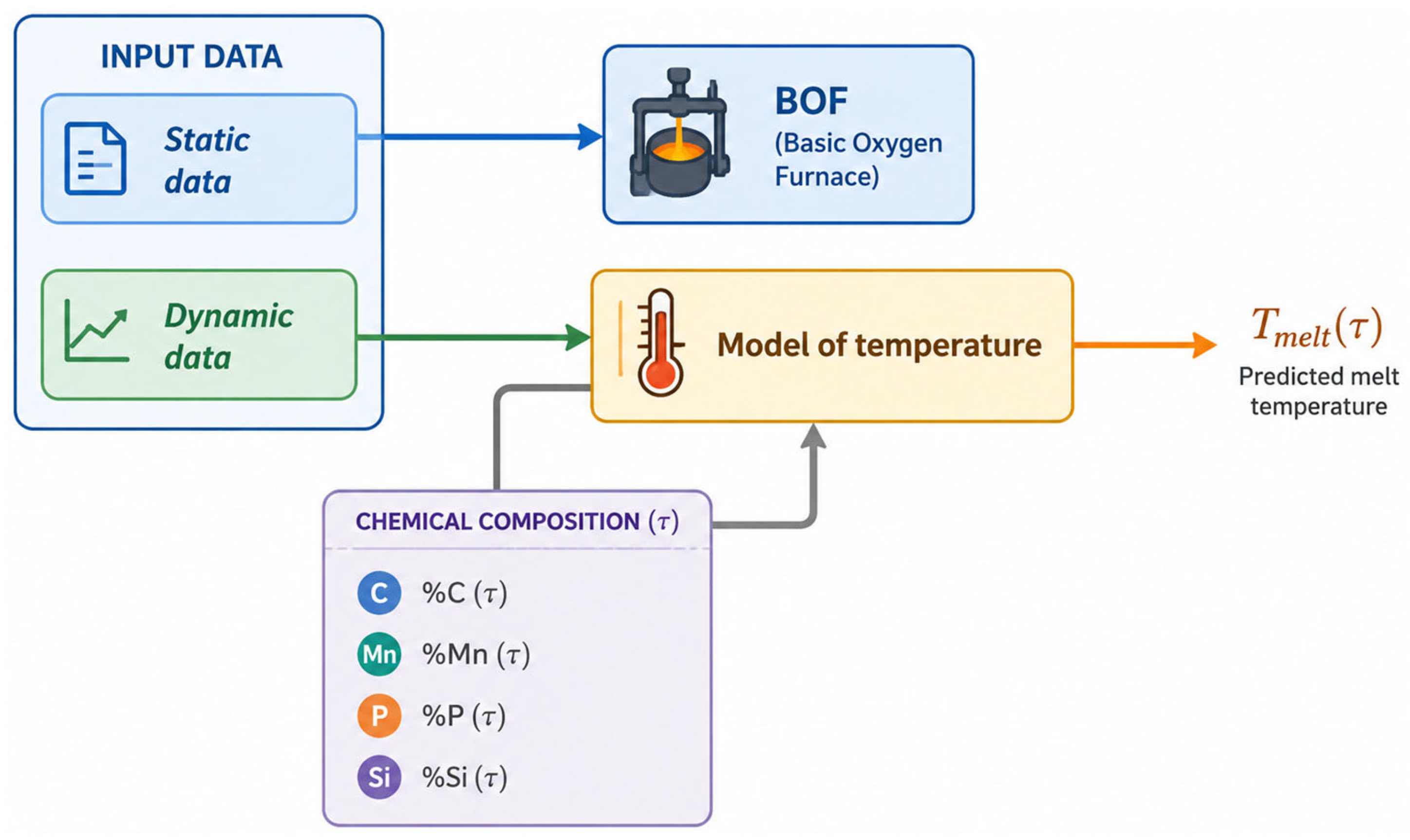
Based on the analysis of the processes occurring in the oxygen converter, a material and heat balance dataset was created to develop a mathematical model for predicting the melt temperature. The input of the model is static and dynamic data. Static data that enter the model before the start of melting include the temperature and weight of pig iron, the weight and type of scrap, the weight of slag-forming additives, etc. Dynamic data primarily include the nozzle height and the volume of blown oxygen (see Figure 2). These data influence the course of the BOF process [41,42].

The heat balance of the BOF process is based on the supplied (7) and consumed (8) heat.

$$Q_{in}=Q_{pigFe}+Q_{exoRe}+Q_{slag}+Q_{fScr}+Q_{fOx}+Q_{fSlf}+Q_{fAir},$$

(7)

where $Q_{pigFe}$ is the physical and latent heat of input pig iron (J), $Q_{exoRe}$ is the heat from exothermic oxidation reactions of elements C, Si, Fe, Mn, and P (J), $Q_{slag}$ is the heat from the reactions during slag formation, $Q_{fScr}$ is the physical heat of the input steel scrap (J), $Q_{fOx}$ is the physical heat of the blown oxygen (J), $Q_{fSlf}$ is the physical heat of the input slag-forming additives (J), and $Q_{fAir}$ is the physical heat of the sucked air (J).

$$Q_{cons}=Q_{fLM}+Q_{fSl}+Q_{dLim}+Q_{fCG}+Q_{fDust}+Q_{hloss},$$

(8)

where $Q_{fLM}$ is the physical and latent heat of the liquid metal (J), $Q_{fSl}$ is the physical and latent heat of the slag (J), $Q_{dLim}$ is the heat needed to decompose limestone (J), $Q_{fCG}$ is the physical heat of the converter gas (J), $Q_{fDust}$ is the physical heat of the dust in the converter gas (J), and $Q_{hloss}$ represents the other heat losses (J).

If the heat balance condition is met, i.e., the equality of the supplied and consumed heat, we can express the metal temperature ($T_{LM}$) as follows:

$$T_{LM}={\displaystyle \frac{Q_{in}-Q_{fSl}-Q_{dLim}-Q_{fCG}-Q_{fDust}-Q_{hloss}-M_{LM}.\left(T_{melt,LM}\left({cp}_{sol,LM}-{cp}_{liq,LM}\right)+Q_{lh,LM}\right)}{M_{LM}.{cp}_{liq,LM}}},$$

(9)

where $M_{LM}$ is the mass of the liquid metal (kg), $T_{melt,LM}$ is the melting temperature of the metal (K), ${cp}_{sol,LM}$ is the specific heat capacity of the solid metal (J/kg/K), ${cp}_{liq,LM}$ is the specific heat capacity of the liquid metal (J/kg/K), and $Q_{lh,LM}$ is the latent heat of fusion of metal (J/kg).

2.1.2. Regression Model

Regression analysis is an approach to identifying and analyzing the relationship between one or more independent variables and a dependent variable. Using regression analysis, we can examine the underlying relationships within the data and build predictive models. Regression analysis can be divided into several types, including simple linear regression, logistic regression, polynomial regression, and multiple regression. The appropriate regression model is determined by the nature of the data and the subject of the study. The purpose of regression analysis is to find the best fit (a line or a curve) between the independent variables and the dependent variable. This best fit is determined using statistical methods that minimize the differences between the expected and actual values in the dataset.

The basic equation of the model is defined as

$$Y_i={\beta }_0+{\beta }_1{x}_{i,1}+{\beta }_2{x}_{i,2}+{\beta }_3{x}_{i,3}+{\beta }_4{x}_{i,4}+{\beta }_5{x}_{i,5}+{\beta }_6{x}_{i,6}+{\beta }_7{x}_{i,7}+{\beta }_8{x}_{i,8}+{\epsilon }_i,$$

(10)

where $Y_i$ is the dependent variable, $x_{i,j}$ are independent variables, ${\beta }_j$ are parameters of the model and ${\epsilon }_i$ is the random error.

The parameter estimates ${\beta }_j$ are obtained using the least squares method by minimizing the sum of squares of the residuals:

$${\displaystyle {\sum }_{i=1}^n}{\epsilon }_i^2={\displaystyle {\sum }_{i=1}^n}{\left(Y_i-{\widehat{Y}}_i\right)}^2.$$

(11)

As mentioned above, the inputs to the model represent the masses of individual scrap categories and the final target melt temperature. The output from the model is the predicted final temperature.

2.1.3. Machine Learning Models

Support Vector Regression (SVR)

Support Vector Regression (SVR) is a kernel-based machine learning method derived from SVM. The objective of SVR is to determine a nonlinear mapping between the input variables and the output variable while minimizing the prediction error and preserving model generalization capability.

The SVR prediction function is defined as [43,44,45]:

$$\widehat{y}\left(\mathrm{x}\right)={\displaystyle {\sum }_{i=1}^{N_s}}\left({\alpha }_i-{\alpha }_i^{*}\right)K\left({\mathrm{x}}_i,\mathrm{x}\right)+b,$$

(12)

where $\mathrm{x}$ is the input vector, ${\mathrm{x}}_i$ are support vectors, ${\alpha }_i \mathrm{a}\mathrm{n}\mathrm{d}$ ${\alpha }_i^{*}$ are Lagrange multipliers, $b$ is the bias term, $K$ is the kernel function, $\mathrm{a}\mathrm{n}\mathrm{d} N_s$ is the number of support vectors.

In this work, the Radial Basis Function (RBF) kernel was employed:

$$K\left({\mathbf{x}}_i,{\mathbf{x}}_j\right)=\mathrm{e}\mathrm{x}\mathrm{p}\left(-\gamma {\Vert {\mathbf{x}}_i-{\mathbf{x}}_j\Vert }^2\right),$$

(13)

where $\gamma$ is the kernel width parameter.

SVR enables nonlinear modeling of the relationship between scrap composition and endpoint temperature while maintaining good robustness against overfitting.

To examine the influence of hyperparameter selection on SVR performance, the model hyperparameters were systematically optimized using Bayesian optimization. The original training and independent testing subsets were retained, and hyperparameter selection was performed exclusively on the training subset using five-fold cross-validation. The testing subset was not used during the optimization. The Gaussian RBF kernel was applied with standardized input variables. Three hyperparameters were optimized: the box constraint $C$, the epsilon-insensitive loss parameter $\epsilon$, and the Gaussian KernelScale. Logarithmic search ranges of $C\in [0.01, 1000]$, $\epsilon \in [0.01, 100]$, and KernelScale $\in [0.01, 1000]$ were considered, with 60 Bayesian optimization evaluations. The selected values were $C$ = 998.56, $\epsilon$ = 0.0374, and KernelScale = 61.82. For the commonly used RBF formulation $K\left({\mathbf{x}}_i,{\mathbf{x}}_j\right)=\mathrm{e}\mathrm{x}\mathrm{p}\left(-\gamma {\Vert {\mathbf{x}}_i-{\mathbf{x}}_j\Vert }^2\right)$, the selected KernelScale corresponds to γ ≈ 1.31 × 10⁻⁴.

Random Forest Regression (RF)

Random Forest (RF) is an ensemble machine learning method based on multiple regression trees. The final prediction is obtained by averaging the outputs of individual decision trees.

The RF prediction model can be expressed as

$$\widehat{y}\left(\mathrm{x}\right)={\displaystyle \frac{1}{M}}{\displaystyle {\sum }_{m=1}^M}{T}_m\left(x\right),$$

(14)

where $M$ is the number of trees and $T_m\left(x\right)$ is the prediction of the $m$-th regression tree.

Each regression tree is trained using a randomly selected subset of the training data and randomly selected input features. This process improves generalization capability and reduces overfitting [46].

Random Forest is particularly suitable for nonlinear industrial processes with complex interactions among variables. Additionally, RF models can naturally capture nonlinear dependencies between scrap composition and endpoint temperature.

Gaussian Process Regression (GPR)

Gaussian Process Regression (GPR) is a probabilistic machine learning method based on Bayesian inference. GPR assumes that the modeled process follows a Gaussian stochastic process.

A Gaussian process is defined as [47]:

$$f\left(\mathrm{x}\right)\sim \mathcal{G}\mathcal{P}\left(m\left(\mathrm{x}\right),k\left(\mathrm{x},{\mathrm{x}}^{\prime }\right)\right),$$

(15)

where $m\left(\mathrm{x}\right)$ is the mean function and $k\left(\mathrm{x},{\mathrm{x}}^{\prime }\right)$ is the covariance kernel function.

The covariance function defines the similarity between observations. In this work, the squared exponential kernel was employed:

$$k\left({\mathbf{x}}_i,{\mathbf{x}}_j\right)={\sigma }_f^2\mathrm{e}\mathrm{x}\mathrm{p}\left(-{\displaystyle \frac{{\Vert {\mathbf{x}}_i-{\mathbf{x}}_j\Vert }^2}{2l^2}}\right),$$

(16)

where ${\sigma }_f^2$ is the signal variance and $l$ is the characteristic length scale.

The predicted output mean is computed as

$$\widehat{y}\left({\mathbf{x}}_{\ast }\right)=K_{\ast }^T{\left(K+{\sigma }_n^{2}I\right)}^{-1}\mathbf{y},$$

(17)

where ${\mathbf{x}}_{\ast }$ is a new input vector, $K$ is the covariance matrix of training samples, $K_{*}$ is the covariance vector between training and test samples, ${\sigma }_n^2$ is the noise variance, and $\mathbf{y}$ is the vector of training outputs.

GPR provides not only the predicted value but also prediction uncertainty, which is advantageous for industrial process analysis and decision support applications.

2.2. Optimization of Steel Scrap

The optimization of steel scrap mass was carried out in two variants. The first variant used a model for optimal adjustment that predicted the final melt temperature based on the mass of individual scrap types and the final target temperature (regression model, machine learning models). The second optimization variant used a simulation model (complex deterministic model) within the optimization system with a model that replaced the real BOF process to optimally adjust the mass of individual scrap types.

2.2.1. Optimization Using Machine Learning Model

After the development and validation of the machine learning prediction models, the best-performing model can be used as a surrogate model for optimization of scrap composition in the BOF process. The primary objective of the optimization procedure is to determine the optimal masses of individual scrap categories such that the predicted endpoint temperature approaches the desired target temperature while satisfying technological and mass-balance constraints.

The developed machine learning model represents a nonlinear mapping of the form

$${\widehat{T}}_{end}=f(x_1,x_2,x_3,x_4,x_5,x_6,x_7,T_{target})$$

(18)

where $x_1,\dots ,x_7$ are the masses of individual scrap categories, T_target is the desired endpoint temperature, $\mathrm{a}\mathrm{n}\mathrm{d} {\widehat{T}}_{end}$ is the predicted endpoint temperature generated by the machine learning surrogate model.

The optimization task is to determine the optimal scrap composition vector so that the predicted endpoint temperature is as close as possible to the desired target temperature.

The optimization criterion (objective function) can be formulated as the minimization of the squared prediction error (19). The objective function penalizes deviations between the predicted endpoint temperature and the required target temperature.

$$J(x)={({\widehat{T}}_{end}\left(x\right)-T_{target})}^2$$

(19)

The optimization problem is subject to several technological constraints. The primary mass-balance constraint is that the total mass of scrap remains constant for each melt (1). In addition to this limitation, lower and upper limits may be set for each scrap category (20). These constraints prevent the optimization algorithm from generating physically unrealistic or technologically unacceptable scrap combinations.

$$x_i^{min}\le x_i\le x_i^{max},$$

(20)

where $x_i^{min}$ is the minimum allowable mass of the $i$-th scrap category and $x_i^{max}$ is the maximum allowable mass of the $i$-th scrap category.

Optimization Procedure

The optimization procedure can be summarized as follows:

• The machine learning surrogate model is trained using historical industrial data.
• The desired target endpoint temperature is specified.
• The optimization algorithm searches for the scrap composition vector satisfying the technological constraints.
• The surrogate model predicts the endpoint temperature for each candidate scrap composition.
• The optimization algorithm minimizes the objective function until convergence is achieved.

The optimization problem was solved in MATLAB R2020a using the constrained nonlinear optimization function fmincon. The Sequential Quadratic Programming (SQP) optimization algorithm was employed because it is well-suited to nonlinear optimization problems with equality, inequality, and bound constraints.

The optimization algorithm iteratively generated scrap mass compositions, which were subsequently evaluated using the trained GPR surrogate model. For each candidate solution, the surrogate model predicted the endpoint temperature, and the optimizer evaluated the corresponding objective function value. Based on this value, the optimization variables were iteratively adjusted in order to minimize the deviation between the predicted and required endpoint temperatures.

The overall optimization procedure can be summarized in the form of pseudocode as follows:

• Load industrial operational data containing $x_1,x_2,x_3,x_4,x_5,x_6,x_7,{\mathrm{a}\mathrm{n}\mathrm{d} T}_{target}$.
• Remove incomplete or invalid observations from the dataset.
• Divide the dataset into training and testing subsets.
• Train the GPR surrogate model (17).
• Define the reference scrap composition x_ref as the mean scrap composition obtained from the training dataset.
• Normalize $x_{ref}$ by the condition (1).
• Set the initial optimization point: $x_0=x_{ref}$.
• Define the objective function (19).
• Use the SQP algorithm implemented in fmincon to solve:

  $$x_{\mathrm{o}\mathrm{p}\mathrm{t}}=\mathrm{a}\mathrm{r}\mathrm{g}\underset{\mathbf{x}}{min} J(\mathbf{x})$$
• Compute the optimized endpoint temperature:

  $${\widehat{T}}_{end, opt}=f_{GPR}(x_{opt},T_{target})$$
• Compute the final temperature error:

  $$e_{opt}={\widehat{T}}_{end, opt}-T_{target}$$
• Return $x_{\mathrm{o}\mathrm{p}\mathrm{t}}$, ${\widehat{T}}_{end,opt}$, and $e_{opt}$.

The SQP algorithm was configured with a maximum of 500 iterations and 10,000 objective function evaluations. The optimality and step tolerances were set to 10⁻⁸, while the constraint tolerance was 10⁻⁶. To assess convergence behavior, the objective function value was recorded at each SQP iteration together with the number of iterations and function evaluations required for termination.

The optimization process terminates when the convergence criteria of the optimization algorithm are satisfied, for example, when the variation of optimization variables between successive iterations becomes sufficiently small, when the gradient of the objective function reaches a sufficiently low value, or when all technological constraints are satisfied within the required tolerance.

In this work, the optimization procedure converged successfully while satisfying both the equality mass-balance constraint and the bound constraints imposed on individual scrap categories. The resulting optimized scrap composition vector ($x_{\mathrm{o}\mathrm{p}\mathrm{t}}$) minimized the deviation between the predicted and required endpoint temperatures.

2.2.2. Optimization Using Deterministic Model of BOF Process

When designing or reconstructing technological objects, we aim to ensure they meet the required criteria, whether economic or technological. When managing a technological process, it is necessary to adhere to the technological procedure and ensure the quality of the resulting product. Ultimately, this means that we strive to optimize the technological object or process. We understand optimization as searching for the best possible option, decision, or control while adhering to technological criteria and limitations.

If a suitable simulation model of the technological process exists, it can be used for optimal process control or for optimizing technological variables.

Optimization using a simulation model can be performed in two ways:

• by comparing simulation studies;
• by using the principle of the “Optimization System with the Model”.

Comparison of simulation studies can be applied in very simple cases when we have to decide on the optimal variant from a known set of variants. For each variant, simulations are performed using a simulation model, and based on the results obtained, the optimal variant is selected according to the specified optimization criterion.

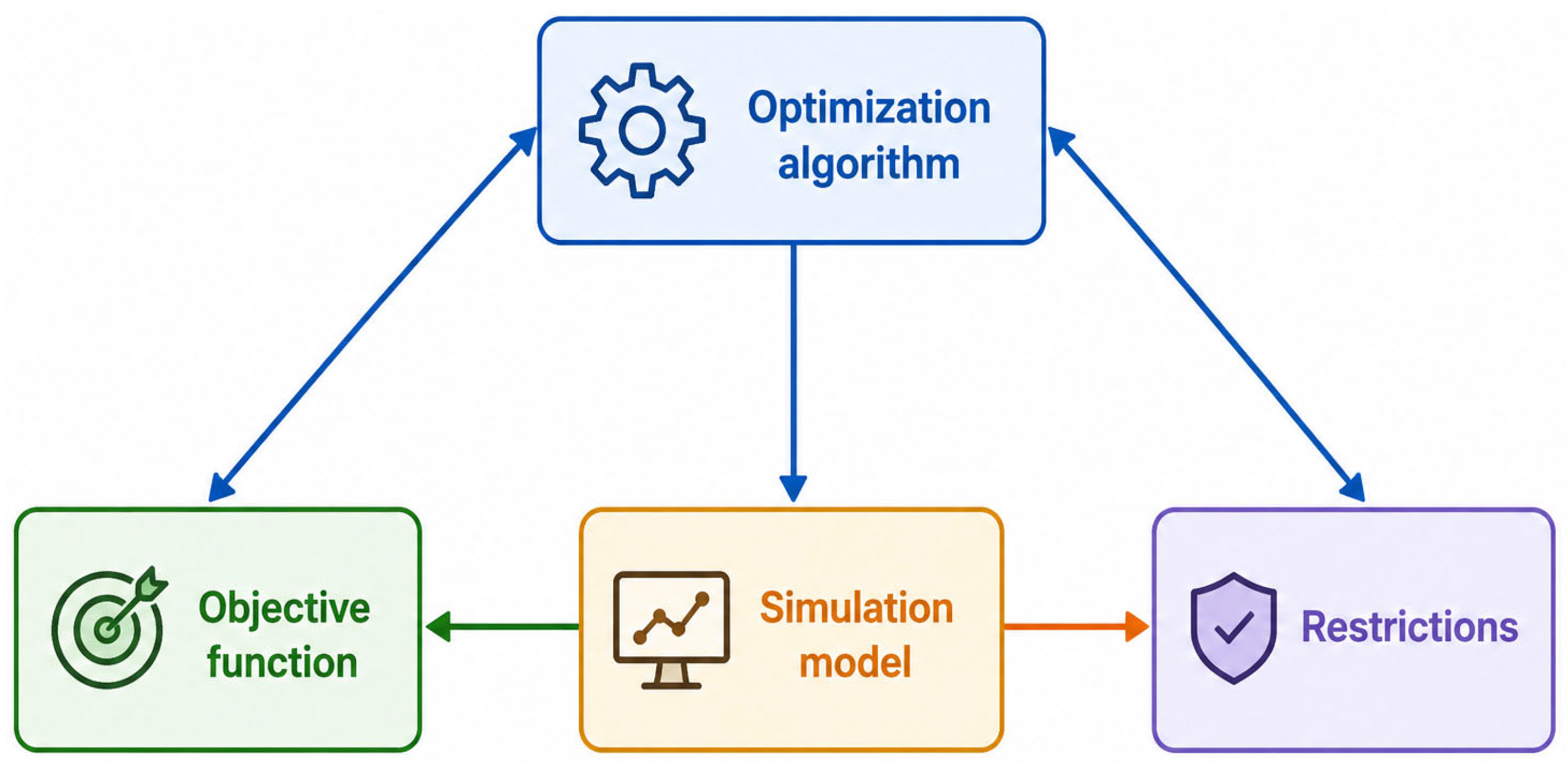
The second way of using simulation models in the optimization of technological processes is the so-called “Optimization System with Model”, which, unlike the aforementioned passive comparison of simulations, includes an optimization algorithm for finding the optimal variant. The principle of the optimization system with the model (see Figure 3) consists of four basic blocks:

• objective function–optimality criterion;
• simulation model;
• constraints;
• optimization algorithm.

Figure 3. System of optimization with the model [48].

Figure 3. System of optimization with the model [48].

Optimized vector

The optimized vector is a vector of variables whose values are changed during the optimization algorithm in such a way as to minimize the objective function. The change in the vector values is ensured by a suitable optimization algorithm (method). In our case, the components of the vector (21) are the masses or percentages of the masses of steel scrap for individual steel scrap classes:

$$\mathit{x}=[x_1 x_2 x_3 x_4 x_5 x_6 x_7].$$

(21)

Objective function

The objective function, which is the goal of optimization, is not expressed explicitly. To calculate its value, a simulation model is used, which, based on the input parameters and the values of the optimized vector, calculates the temperature of the steel at the end of the melt. Subsequently, the objective function (22) is calculated as the sum of the deviations between the steel temperature predicted by the model and the target temperature at the end of the melt for individual melts.

$$J(x)={\displaystyle {\sum }_{i=1}^n}\left|T_{mod}^i\left({\tau }_k\right)-T_{target}^i\left({\tau }_k\right)\right|,$$

(22)

where $T_{mod}^i\left({\tau }_k\right)$ is the model endpoint temperature, $T_{target}^i\left({\tau }_k\right)$ is the target endpoint temperature, and n is the number of melts.

Simulation model

The simulation model replaces (imitates) the real BOF process, and in our case, we use the deterministic model described in Section 2.1.1.

Restrictions

The constraints are checked after each simulation that we perform within the optimization system with the model. If any constraints are exceeded or violated, it is necessary to account for this in the optimization algorithm. In our case, these are the constraints on the total mass of steel scrap (1) and the mass limits for individual scrap types (20). After calculating the new values of the optimized vector (21) according to the optimization algorithm, the percentage recalculation of the individual scrap weights occurs so that the condition of the total scrap weight is ensured (1).

Optimization algorithm

The gradient method was chosen as the optimization algorithm. It is an iterative method that, based on the last approximation of a point, searches for the next point at which the objective function takes a smaller value than at the last point. From the last approximation, a straight line is drawn along which the value of the function decreases in the vicinity of this point, and a point at which the value of the function is smaller is selected on it according to the rule.

When searching for a minimum, we choose the direction in which the function decreases most. At a given point, this is the direction opposite to the gradient direction, and the approximation of the next iteration point is given by Formula (23).

$${\overline{x}}_{k+1}={\overline{x}}_k-h·\nabla f\left(x_k\right),$$

(23)

where $\overline{x}$ is the optimized vector, $\nabla f\left(x_k\right)$ is the gradient, k is the optimization step, and $h$ is the weight of the gradient.

In the gradient method, we keep the weight of the gradient $h$ constant and reduce it only if the objective function does not decrease after the optimization step.

The algorithm of the gradient method is as follows:

• Setting the reference composition of the optimized vector (21).
• Optimization step k = 0; step of method h = const.
• The value of the objective function $J\left(x_k\right)$ is calculated/determined by (22).
• Calculation of the gradient components $\nabla f\left(x_k\right)$.
• New values of the optimized vector are calculated by (23).
• The value of the objective function $J\left(x_{k+1}\right)$ is calculated/determined.
• Comparison of the objective function values. If $J\left(x_k\right)$ < $J\left(x_{k+1}\right)$, the step of method $h={\displaystyle \frac{h}{2}}$, and continue to step 5; if not, continue to step 8.
• The termination condition is checked, which may be the prescribed number of steps of the optimization method or the accuracy of the difference between the objective function values in the last two steps. If the condition is not met, set k = k + 1 and continue with point 3.

2.3. Dataset Description and Preparation

The dataset used in this study was derived from operational records of 180 industrial BOF heats. For each heat, the available process records included the masses of seven scrap categories, denoted as $x_1,\dots ,x_7$, and the prescribed target endpoint temperature $x_8=T_{target}$. These variables represent the industrial-data component of the dataset used in the present study.

It is important to distinguish these industrial input variables from the output variable used to train the machine learning surrogate models. The response variable $Y$ was not the directly measured endpoint temperature of the corresponding industrial heat. Instead, $Y$ was generated by the existing deterministic BOF process model evaluated for the respective process conditions. Consequently, the dataset used for ML training combines industrial operational inputs with model-generated endpoint temperatures. The SVR, RF, and GPR models should therefore be interpreted as surrogate models approximating the deterministic BOF process model rather than as models independently trained against measured industrial endpoint temperatures.

Before model training, the dataset was checked for incomplete numerical records. Observations containing missing values in any of the seven scrap variables, the target temperature, or the model-generated output temperature were excluded from further processing. The total scrap mass was also checked for consistency with the prescribed mass-balance condition. After preprocessing, the valid observations were randomly divided into training and testing subsets using an 80:20 ratio with a fixed random seed, resulting in 144 training observations and 36 testing observations. The same data partition was used for the comparison of the investigated machine learning models.

The industrial operating data considered in this study originate from a 180 t top-blown LD converter. The converter has an unlined vessel volume of approximately 300 m³. Under standard operating conditions, the main oxygen blowing period is approximately 15–16.5 min, while the total heat duration is typically 43–50 min. The oxygen consumption is approximately 8300–9200 Nm³ per heat. The principal operating variables affecting the process include the amount and temperature of hot metal, scrap charge, slag-forming additions, oxygen flow, and oxygen lance position. These operating characteristics correspond to the converter process investigated in our previous work [5].

3. Results

The achieved research results are presented at two levels. In the first part, the results of the surrogate models for predicting the final melt temperature are presented. Subsequently, the results of two approaches to optimizing the mass of steel scrap are presented.

3.1. Results of the Models for Prediction

The investigated models were compared using training and testing datasets. The comparison included numerical performance metrics and graphical visualization of the reference model outputs and the corresponding predicted endpoint temperatures.

The evaluated models include:

• Regression model (RM),
• ML model–Support Vector Regression (SVR),
• ML model–Random Forest Regression (RF),
• ML model–Gaussian Process Regression (GPR).

The surrogate models were trained using a dataset constructed from operational records of 180 industrial BOF heats. The input variables consisted of the industrial scrap masses and target endpoint temperature, whereas the output variable corresponded to the endpoint temperature generated by the deterministic BOF process model. The dataset was divided into training and testing subsets using an 80:20 ratio, resulting in 144 training and 36 testing observations.

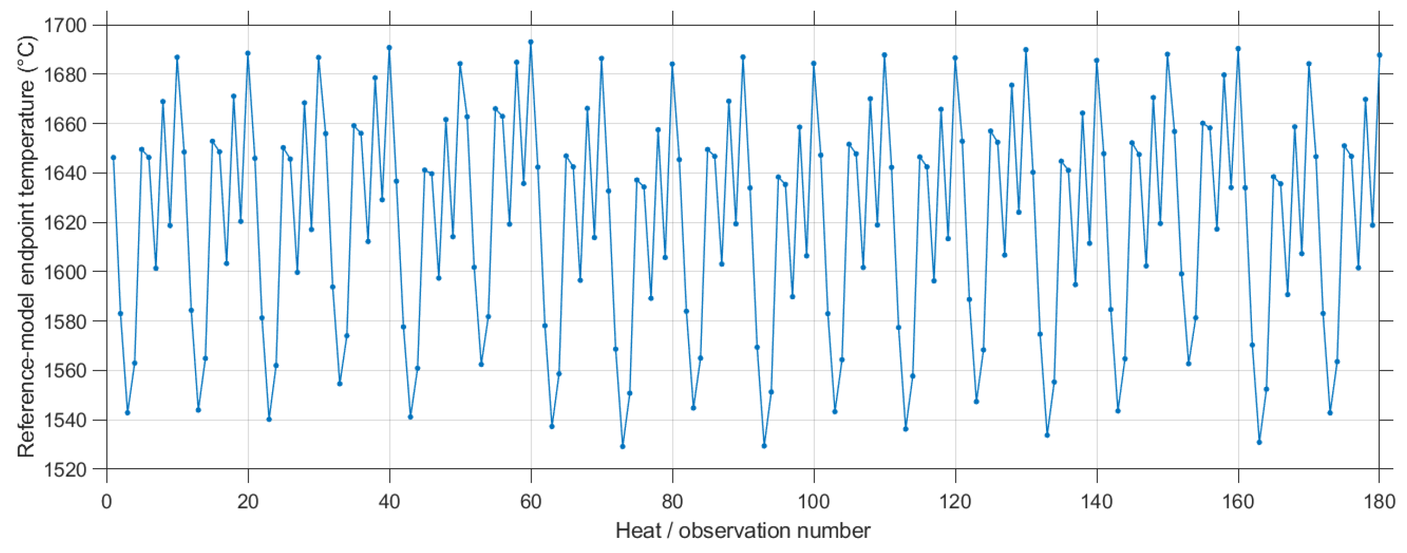
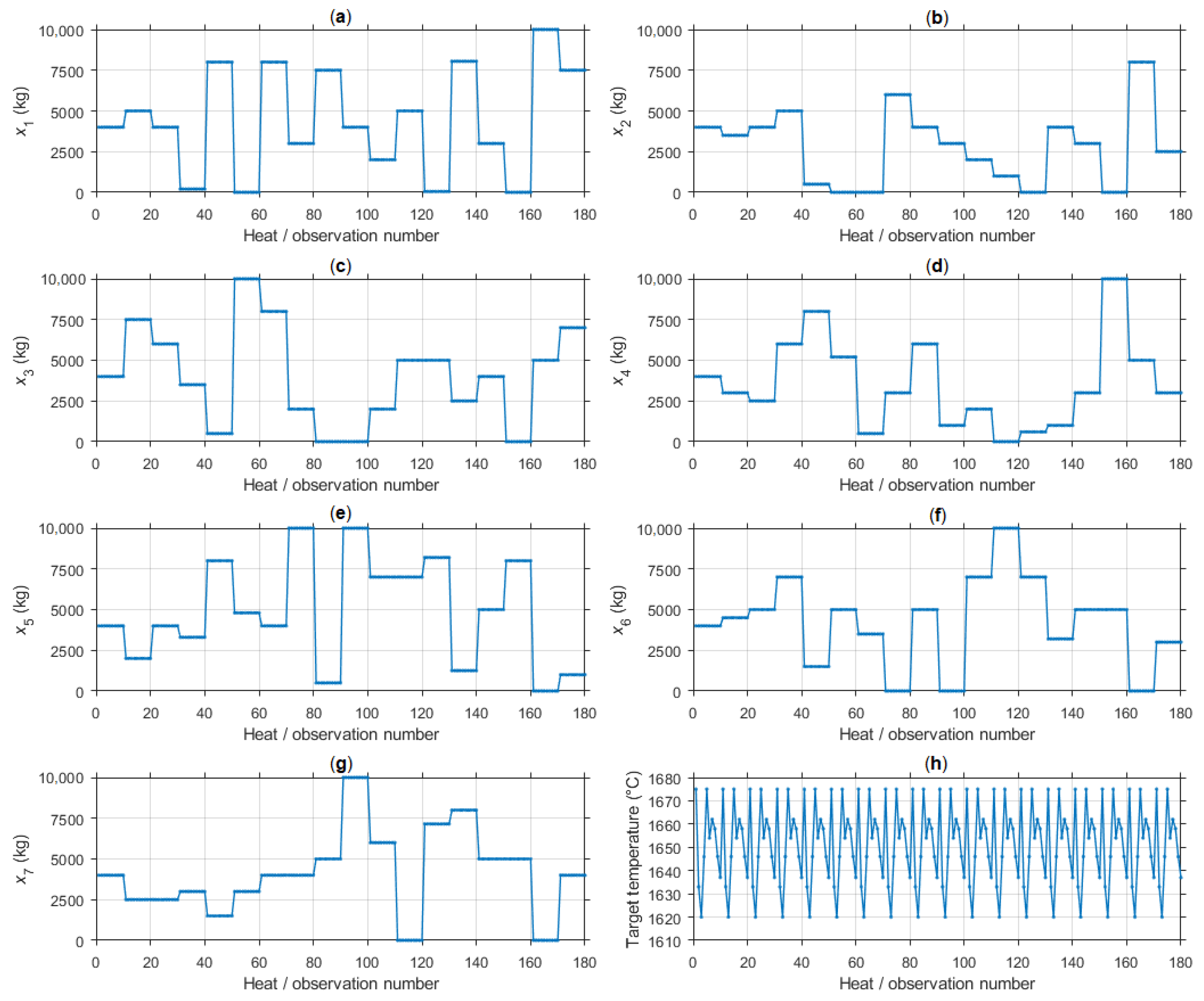
The primary objective was to evaluate the capability of the individual ML approaches to approximate the input–output mapping represented by the deterministic BOF process model. The following figures show the complete dataset used for regression and ML model development. Figure 4 shows the model-generated endpoint temperature $Y$ used as the output variable for training and testing the surrogate models. Figure 5 presents the corresponding input variables, comprising the masses of the seven scrap categories ($x$) and the target endpoint temperature.

3.1.1. Regression Model

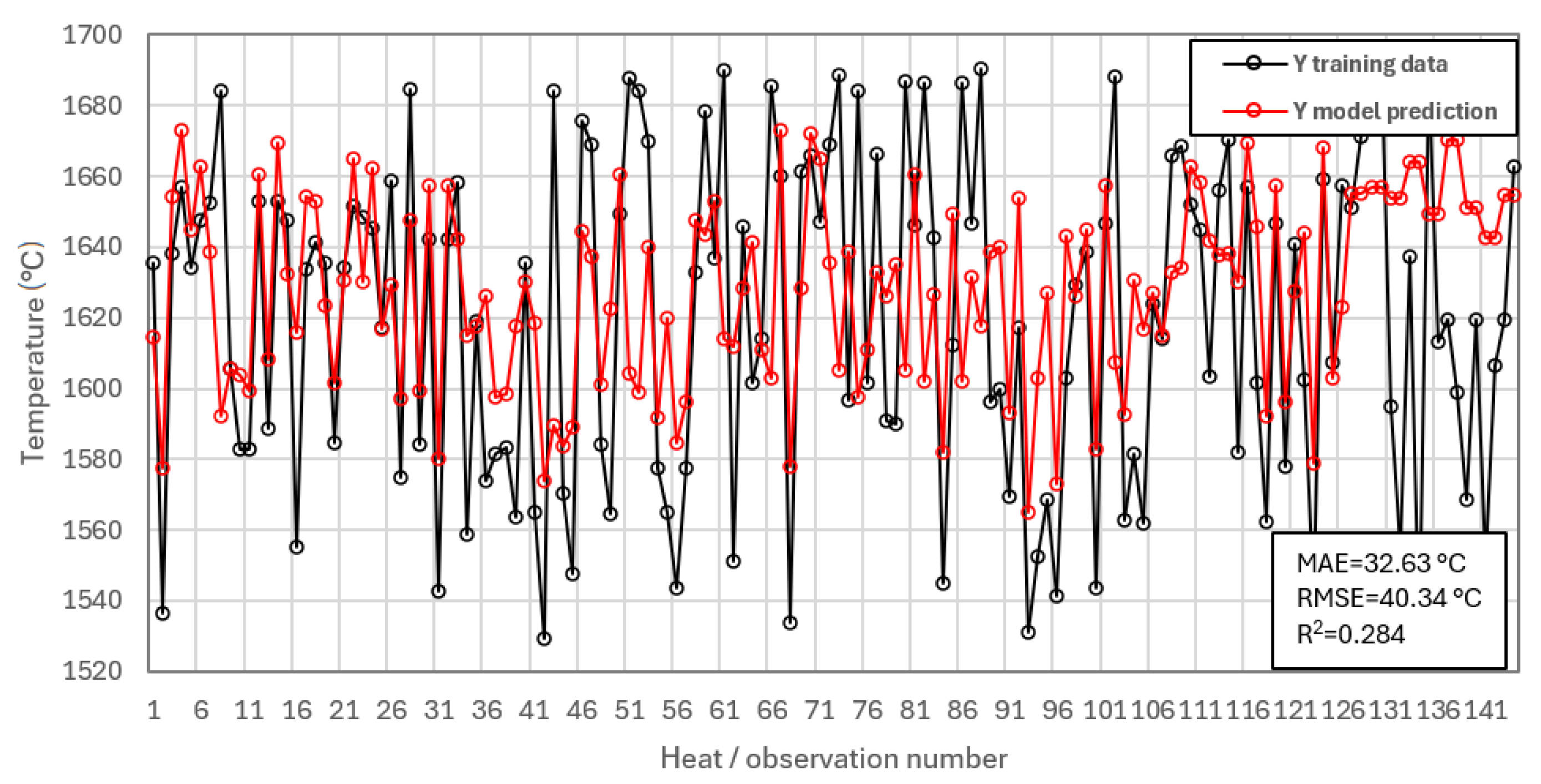
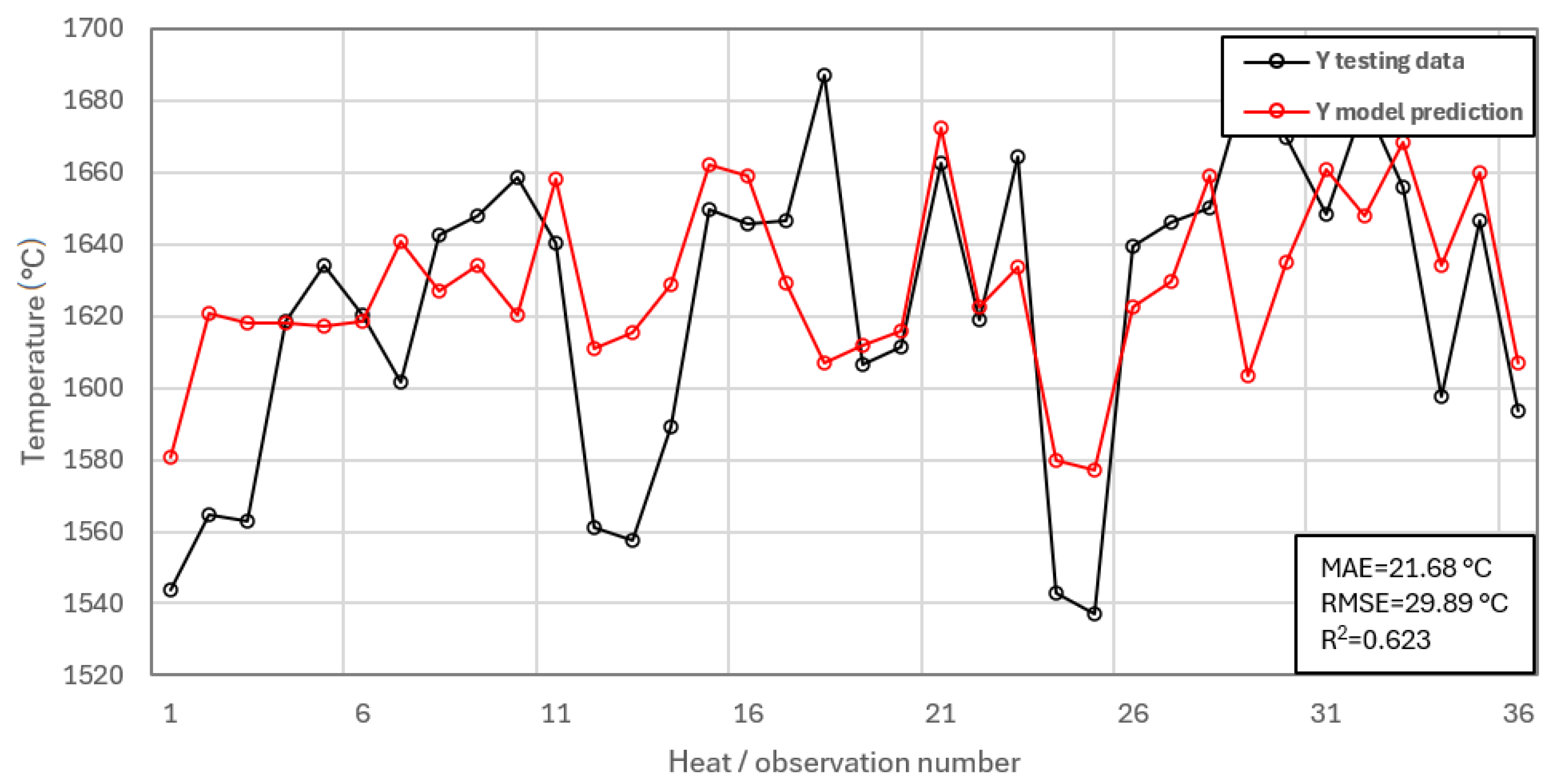
Figure 6 and Figure 7 present the prediction performance of the regression model for the training and testing datasets, respectively.

The presented results of the regression model showed that the model achieved a relatively low approximation ability. The coefficient of determination $R^2$ reached a value of 0.623, and the RMSE value was approximately 29.89 °C.

3.1.2. Machine Learning Models

Support Vector Regression (SVR)

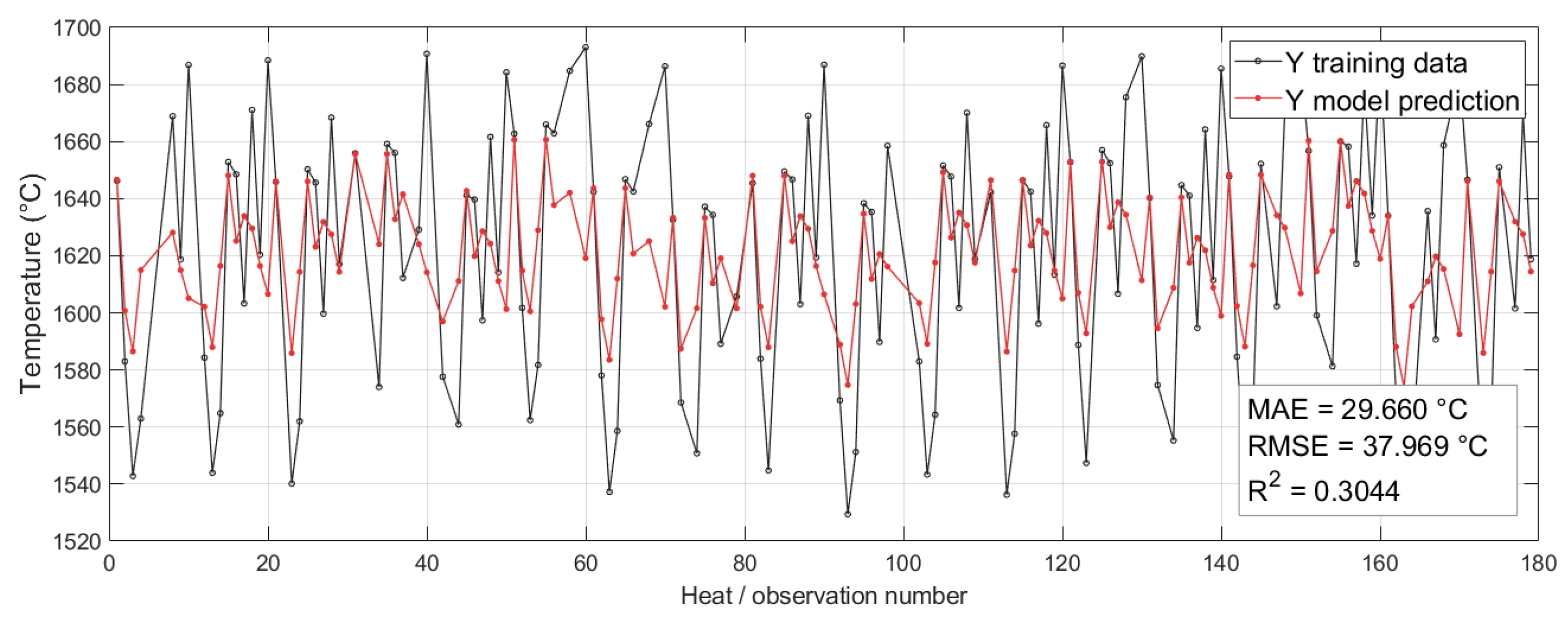
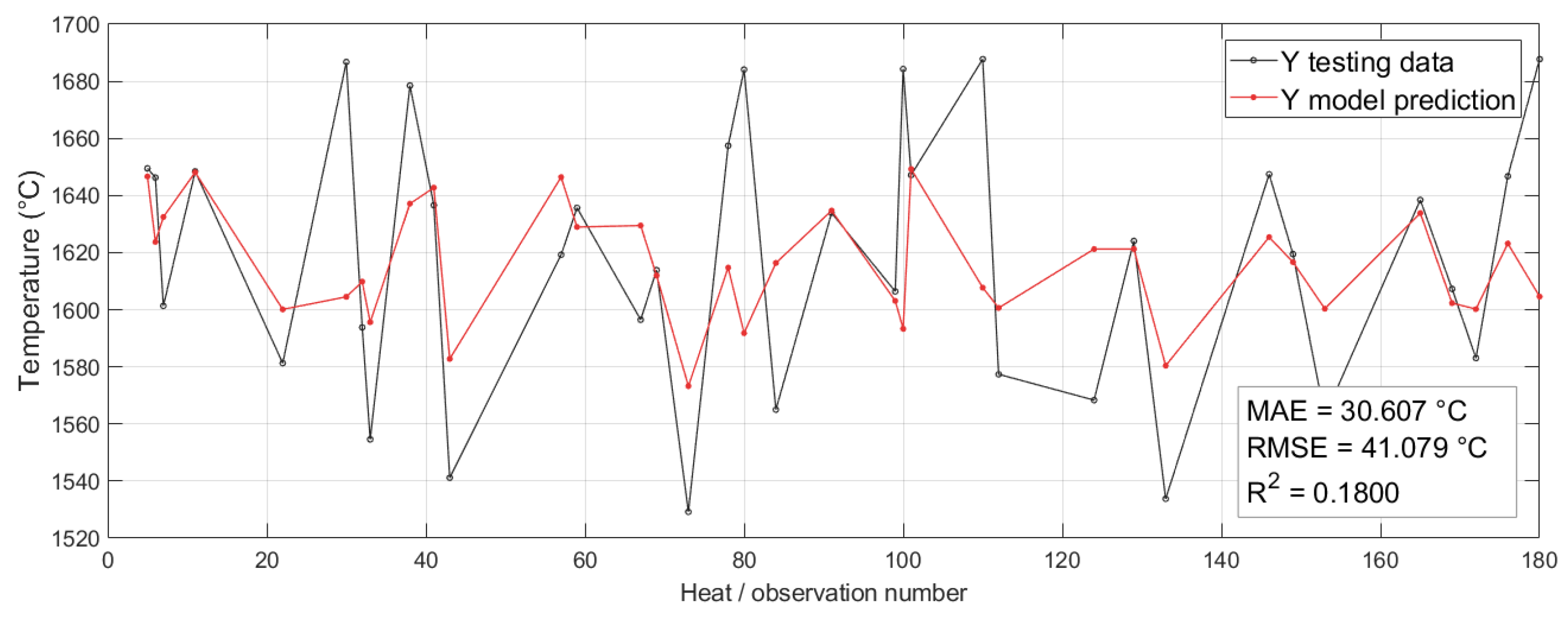
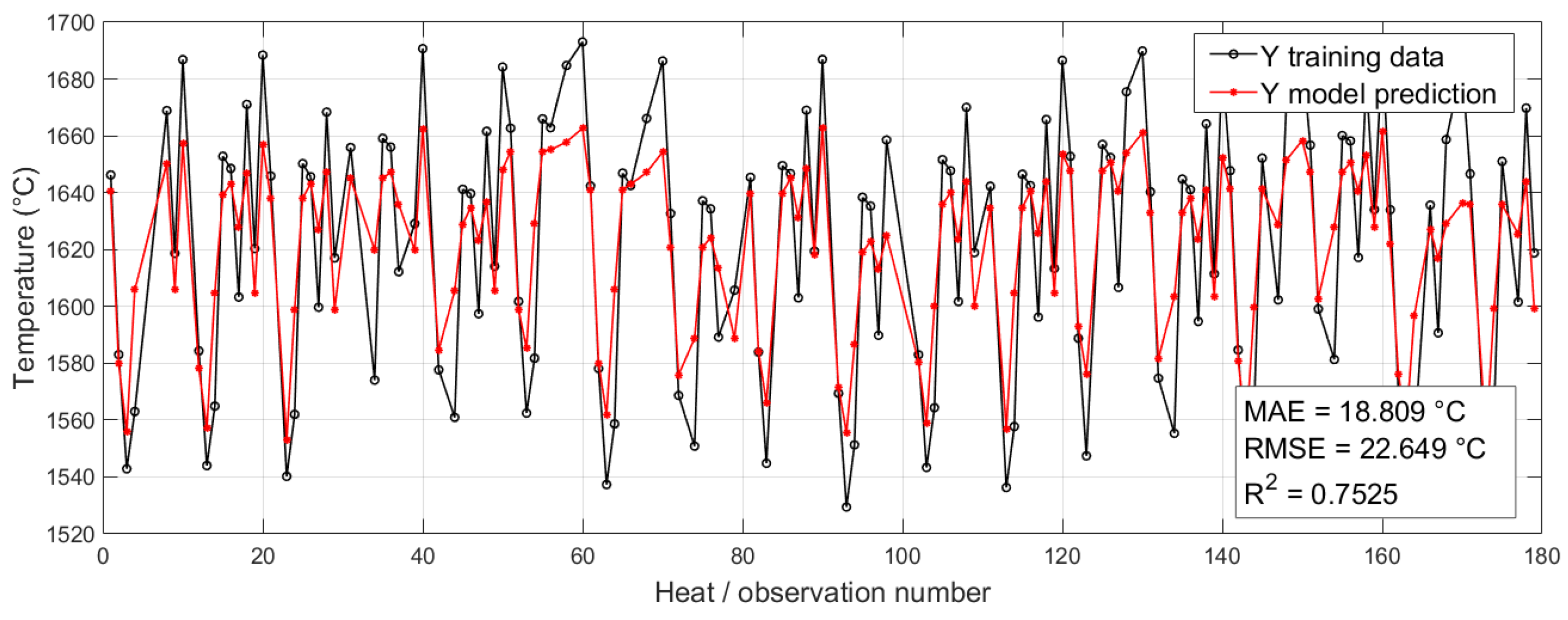
Figure 8 and Figure 9 present the prediction performance of the Support Vector Regression model for the training and testing datasets, respectively.

The SVR model achieved relatively poor approximation capability compared to the other investigated approaches. The results suggest that the selected SVR configuration was unable to sufficiently capture the nonlinear relationships between scrap composition and endpoint temperature. After systematic hyperparameter optimization, the SVR model achieved a test MAE of 30.61 °C and an RMSE of 41.08 °C, with $R^2$ = 0.18. The positive but relatively low coefficient of determination indicates that hyperparameter tuning improved the generalization performance of the model; however, the SVR predictions still explained only a limited proportion of the variability in the independent testing data.

Random Forest Regression (RF)

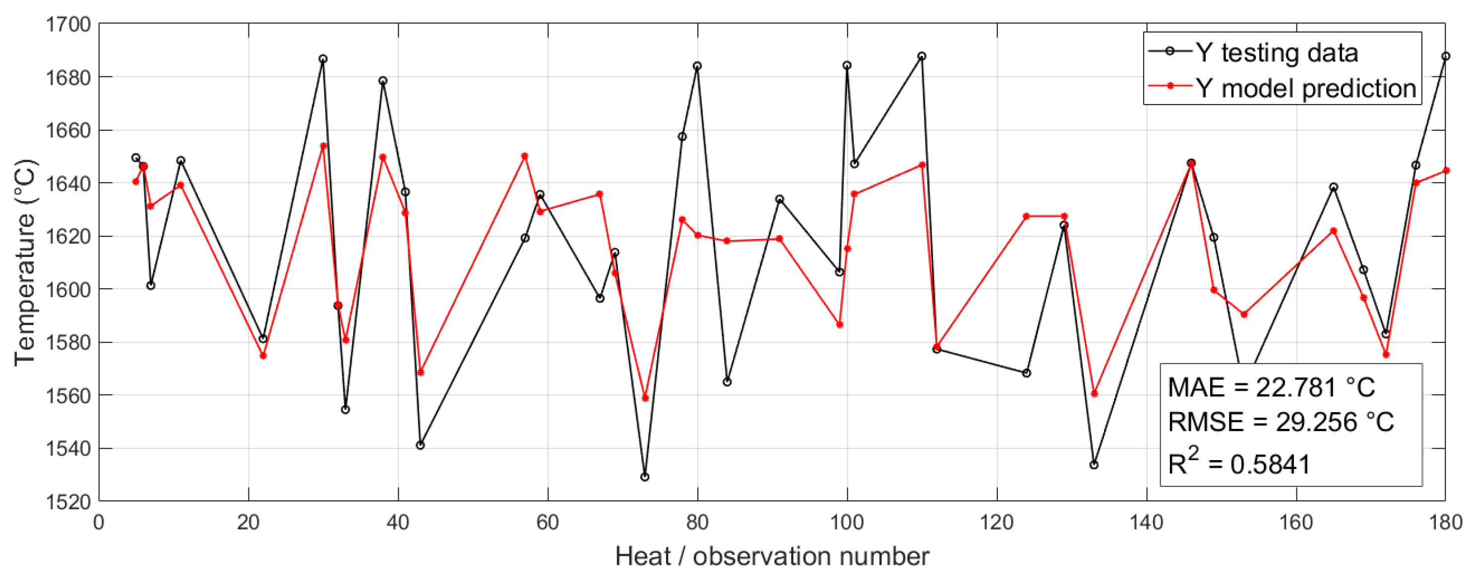
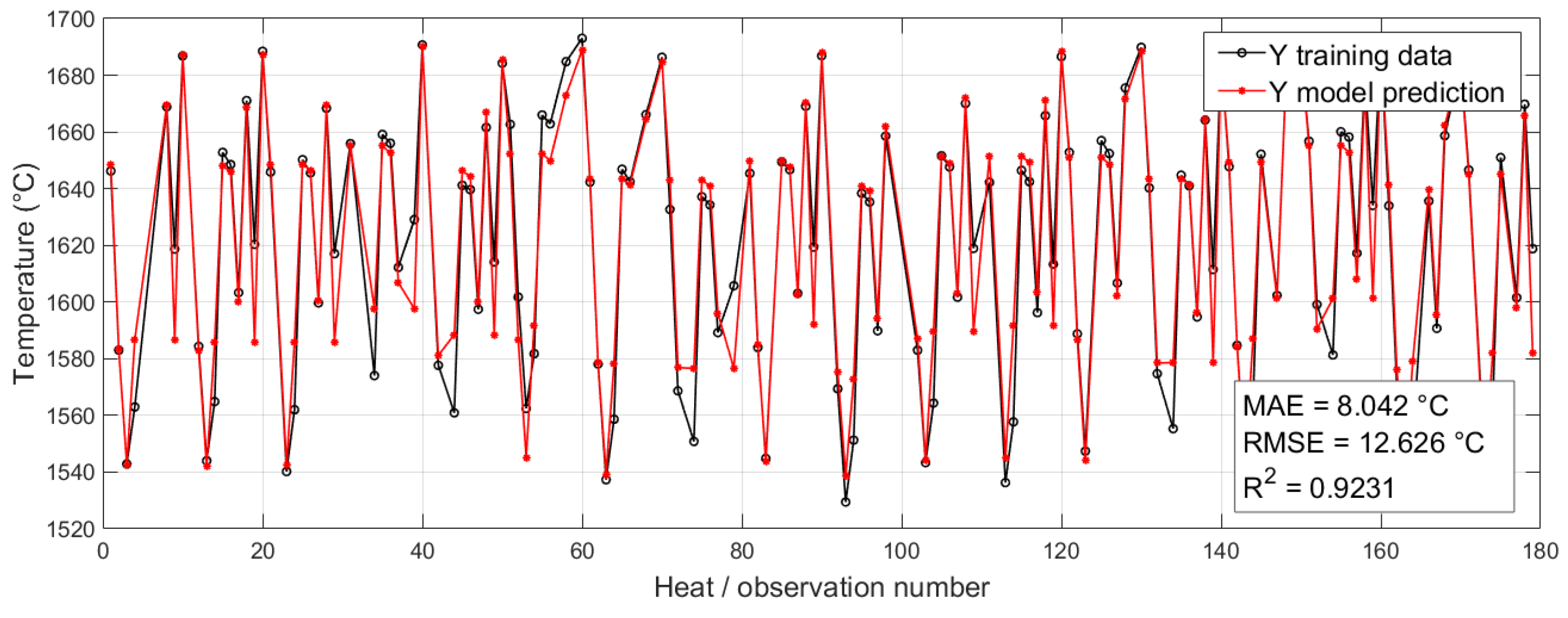
Figure 10 and Figure 11 present the prediction performance of the Random Forest Regression model for the training and testing datasets, respectively.

The Random Forest model achieved significantly better predictive performance than the SVR model. The testing coefficient of determination ($R^2$) was 0.584, and the testing RMSE was reduced to 29.26 °C. The Random Forest model demonstrated improved capability to capture nonlinear dependencies and interactions among input variables. The ensemble structure of the RF model also improved robustness against overfitting.

Gaussian Process Regression (GPR)

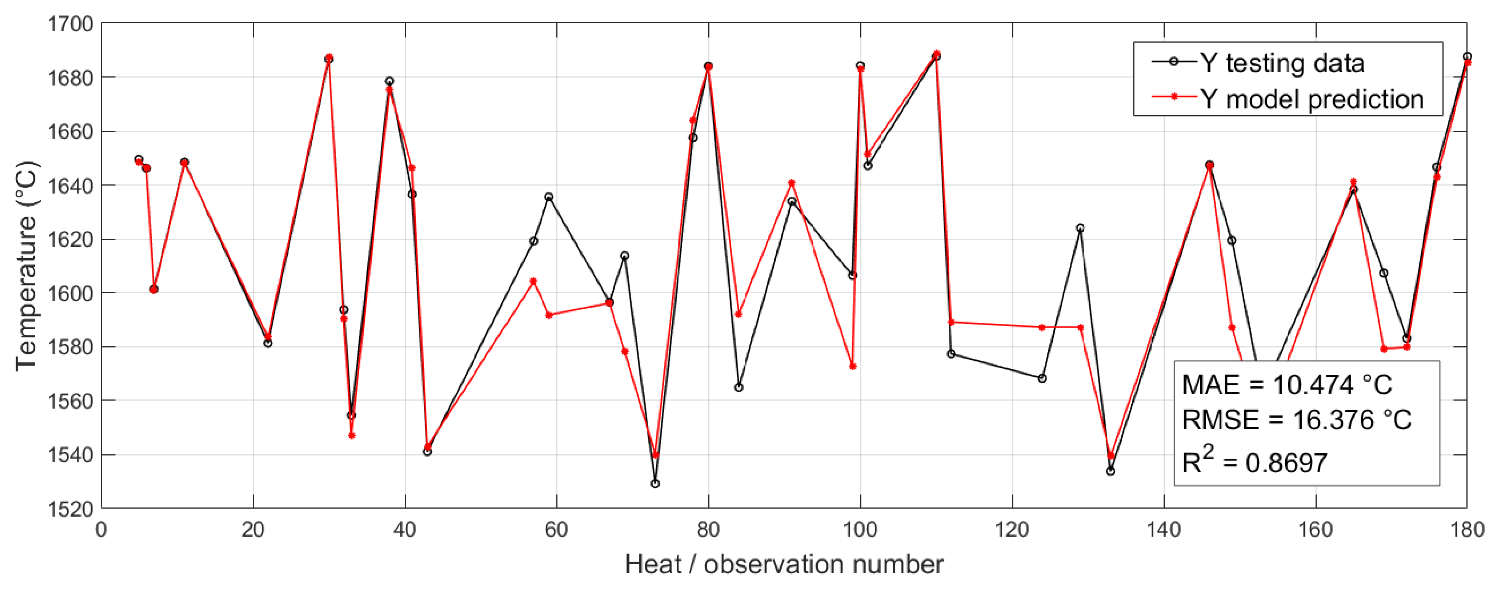
Figure 12 and Figure 13 present the prediction performance of the Gaussian Process Regression model for the training and testing datasets, respectively.

Among all investigated approaches, the Gaussian Process Regression model achieved the best prediction performance. The obtained testing metrics were $R^2$ = 0.870 and RMSE = 16.38 °C. The achieved approximation accuracy indicates that the GPR model was able to successfully reproduce the nonlinear input–output behavior represented by the deterministic BOF process model. Moreover, the relatively small difference between training and testing metrics suggests good generalization capability and limited overfitting.

Comparison of Regression and ML Models

The overall numerical comparison of all investigated melt temperature prediction models is summarized in

Table 1. Predictive performance of the investigated models on the independent test dataset.

Model	MAE	RMSE	R2
Regression	21.68	29.89	0.62
Tuned SVR	30.61	41.08	0.18
RF	22.78	29.26	0.58
GPR	10.47	16.38	0.87

.

In addition to the aggregate performance metrics, pairwise statistical comparisons were performed for the ML models using the absolute prediction errors obtained on the same 36 test observations. The normality of the paired error differences was not rejected by the Lilliefors test ($p$ > 0.05 for all comparisons); therefore, paired t-tests were applied. A significance level of $\alpha$ = 0.05 was adopted; thus, a p-value (probability that the result occurred by chance) below 0.05 was considered to indicate a statistically significant difference between the paired model errors. GPR exhibited significantly lower absolute prediction errors than both the tuned SVR ($p$ = 0.0014) and RF ($p$ = 0.0041).

RF also showed significantly lower errors than the tuned SVR ($p$ = 0.0075). All differences remained statistically significant after Holm–Bonferroni correction for multiple pairwise comparisons (adjusted $p$ < 0.01). These results further support the selection of GPR as the surrogate model for the subsequent optimization.

Pairwise comparison of absolute prediction errors for the ML models using paired t-tests: GPR vs. tuned SVR, $p$ = 0.0014; GPR vs. RF, $p$ = 0.0041; tuned SVR vs. RF, $p$ = 0.0075. Holm–Bonferroni adjusted p-values were 0.0042, 0.0082, and 0.0082, respectively.

The results show that the SVR model exhibited relatively large prediction errors and limited generalization capability compared with the remaining models. The Random Forest model considerably improved prediction accuracy but still produced larger prediction errors than the GPR model. Among the investigated approaches, GPR achieved the best compromise between prediction accuracy and generalization capability.

The comparison clearly demonstrates the superior performance of the Gaussian Process Regression model. GPR achieved the lowest prediction errors and the highest coefficient of determination among all investigated models. The Regression and Random Forest models also achieved acceptable prediction performance and outperformed the SVR model in terms of the reported aggregate metrics. However, their prediction accuracy remained lower compared to that of GPR. The SVR model achieved the weakest performance. In comparison with RF and GPR, SVR therefore remained the least accurate of the three investigated machine learning models for the present dataset.

According to Table 1, the GPR model achieved the lowest prediction errors and the highest coefficient of determination among all investigated methods. Therefore, it was selected as the surrogate model for the subsequent optimization study.

3.2. Results of the Optimization of Steel Scrap

The results of optimizing the steel scrap mass are presented in two parts: optimization using the best surrogate ML model and optimization using the deterministic model.

3.2.1. Optimization Using Machine Learning Model

Based on the comparative analysis of the investigated machine learning approaches, the Gaussian Process Regression (GPR) model achieved the best prediction performance and was therefore selected as the surrogate model for subsequent scrap composition optimization.

The optimization objective was to determine the optimal masses of individual scrap categories such that the predicted endpoint temperature approached the desired target temperature while satisfying the technological mass-balance constraint.

The developed optimization framework was tested in the first step for a target endpoint temperature of $T_{target}$ = 1650 °C.

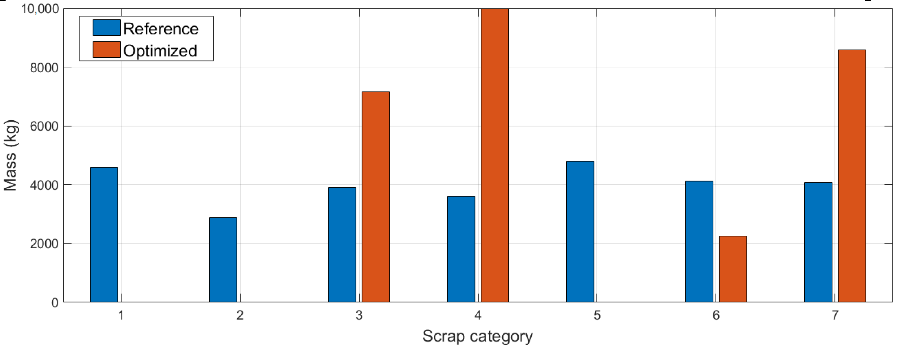
The initial reference scrap composition was obtained as the mean value of the training dataset. Using this reference composition, the GPR surrogate model predicted the endpoint temperature as ${\widehat{T}}_{end, ref}$ = 1616.63 °C, which corresponds to a temperature deviation $e_{ref}$ = −33.37 °C. After optimization, the predicted endpoint temperature achieved by the GPR surrogate model was ${\widehat{T}}_{end, opt}$ = 1648.20 °C, which corresponds to a final prediction error of $e_{opt}$ = −1.80 °C. The optimization procedure therefore reduced the temperature prediction error from 33.37 °C to 1.80 °C.

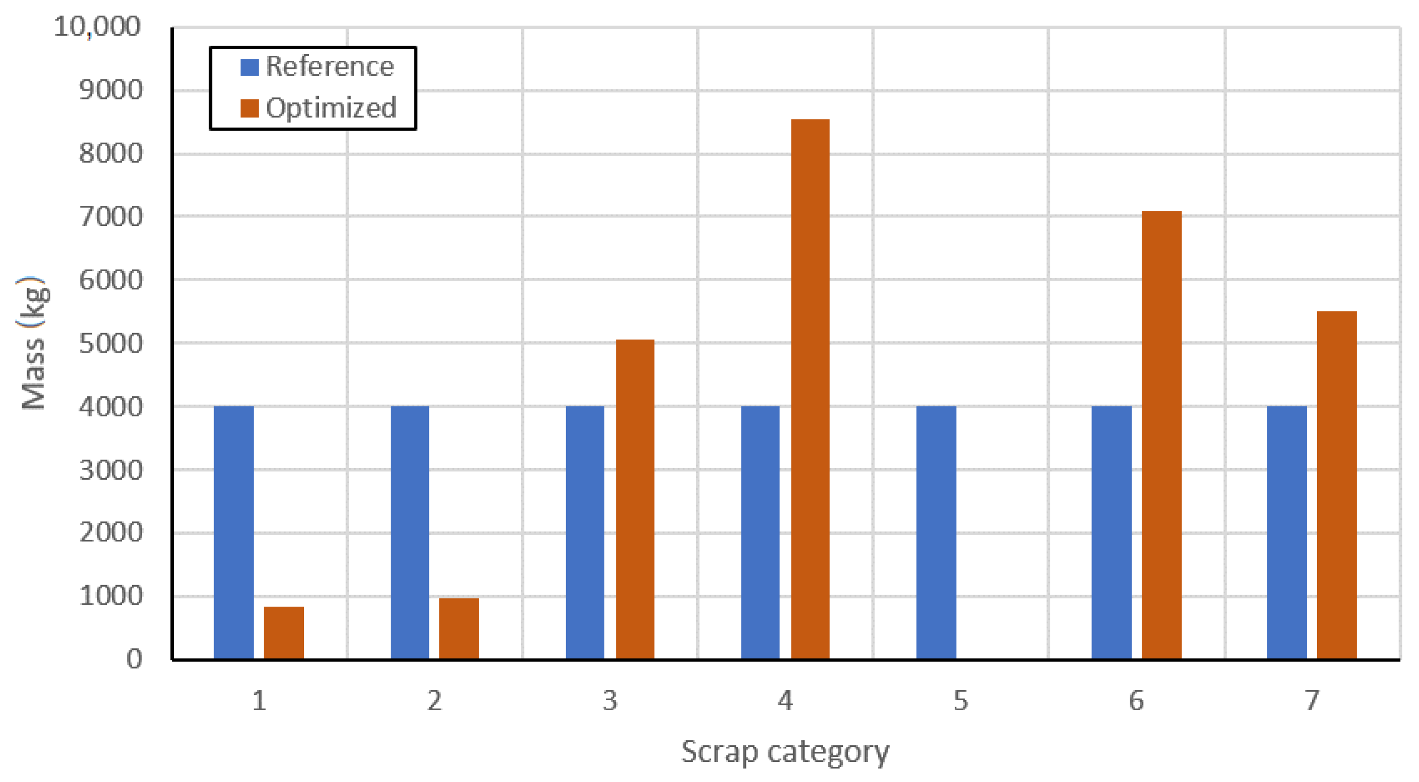
Figure 14 shows the comparison between the reference and optimized scrap compositions obtained using the GPR-based optimization framework.

Although noticeable changes can be observed for several scrap categories, the optimized solution satisfies the imposed mass-balance and variable-bound constraints. However, several variables approach their lower or upper bounds because the present optimization formulation does not include plant-specific restrictions on individual scrap categories. Therefore, these results should be interpreted as model-based optimization solutions within the defined feasible region rather than directly applicable industrial scrap recipes.

In order to evaluate the robustness of the proposed GPR-based optimization framework, the optimization procedure was repeated for multiple target endpoint temperatures in the range from 1620 °C to 1690 °C with a step of 5 °C. For each target temperature, the same reference scrap composition was used as the initial point, and the optimization algorithm searched for the optimal values of $x_1,\dots ,x_7$ under the mass-balance constraint (1).

The numerical results are summarized in

Table 2. Multi-target optimization results using the GPR surrogate model.

${\mathit{T}}_{\mathit{t}\mathit{a}\mathit{r}\mathit{g}\mathit{e}\mathit{t}}$ (°C)	${\widehat{\mathit{T}}}_{\mathit{r}\mathit{e}\mathit{f}}$ (°C)	${\mathit{e}}_{\mathit{r}\mathit{e}\mathit{f}}$ (°C)	${\widehat{\mathit{T}}}_{\mathit{o}\mathit{p}\mathit{t}}$ (°C)	${\mathit{e}}_{\mathit{o}\mathit{p}\mathit{t}}$ (°C)	Improvement (°C)
1620	1572.52	−47.48	1607.51	−12.49	34.99
1625	1579.92	−45.08	1614.35	−10.65	34.43
1630	1587.33	−42.67	1621.17	−8.83	33.84
1635	1594.72	−40.28	1627.96	−7.04	33.24
1640	1602.08	−37.92	1634.73	−5.27	32.66
1645	1609.38	−35.62	1641.49	−3.51	32.10
1650	1616.63	−33.37	1648.20	−1.80	31.57
1655	1623.80	−31.20	1654.84	−0.16	31.05
1660	1630.87	−29.13	1660.00	0.00	29.13
1665	1637.84	−27.16	1665.00	0.00	27.16
1670	1644.69	−25.31	1670.00	0.00	25.31
1675	1651.40	−23.60	1675.00	0.00	23.60
1680	1657.96	−22.04	1680.00	0.00	22.04
1685	1664.37	−20.63	1685.00	0.00	20.63
1690	1670.60	−19.40	1690.00	0.00	19.40

. The table compares the predicted endpoint temperature obtained using the reference scrap composition with the optimized prediction obtained after constrained optimization.

The reference composition systematically underestimates the target endpoint temperature over the whole investigated range. In contrast, the optimized solution significantly shifts the predicted endpoint temperature toward the ideal line (${\widehat{T}}_{opt}$ = $T_{target}$). For target temperatures above approximately 1660 °C, the optimized prediction practically coincides with the target temperature.

The absolute error of the reference composition decreases from approximately 47.48 °C at $T_{target}$ = 1620 °C to 19.40 °C at $T_{target}$ = 1690 °C. After optimization, the absolute error is substantially reduced over the entire range. For target temperatures from 1660 °C to 1690 °C, the final error is practically zero. The improvement ranges from approximately 34.99 °C for the lowest investigated target temperature to 19.40 °C for the highest target temperature. This confirms that the optimization framework consistently improves the predicted endpoint temperature for all investigated operating points.

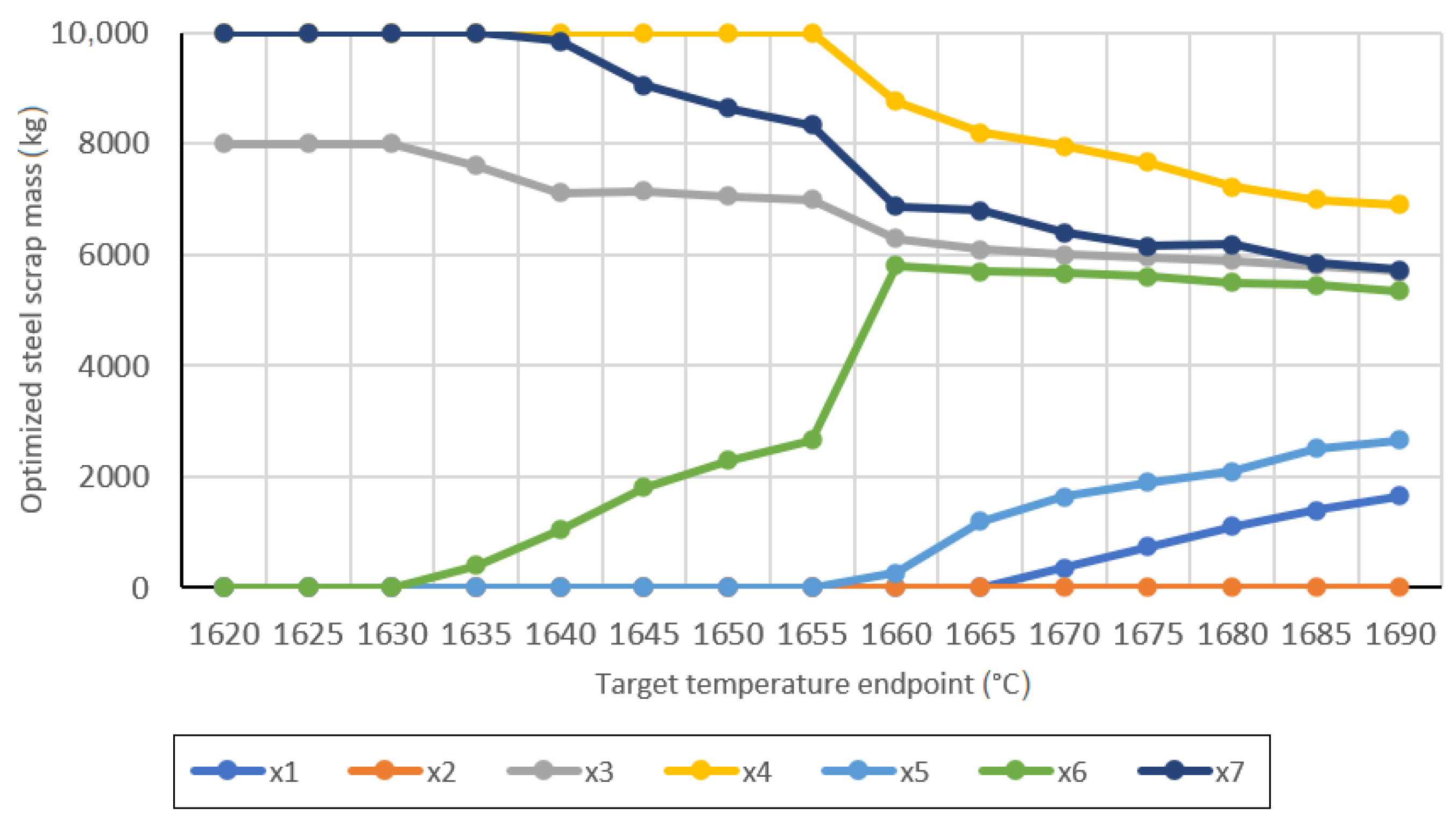
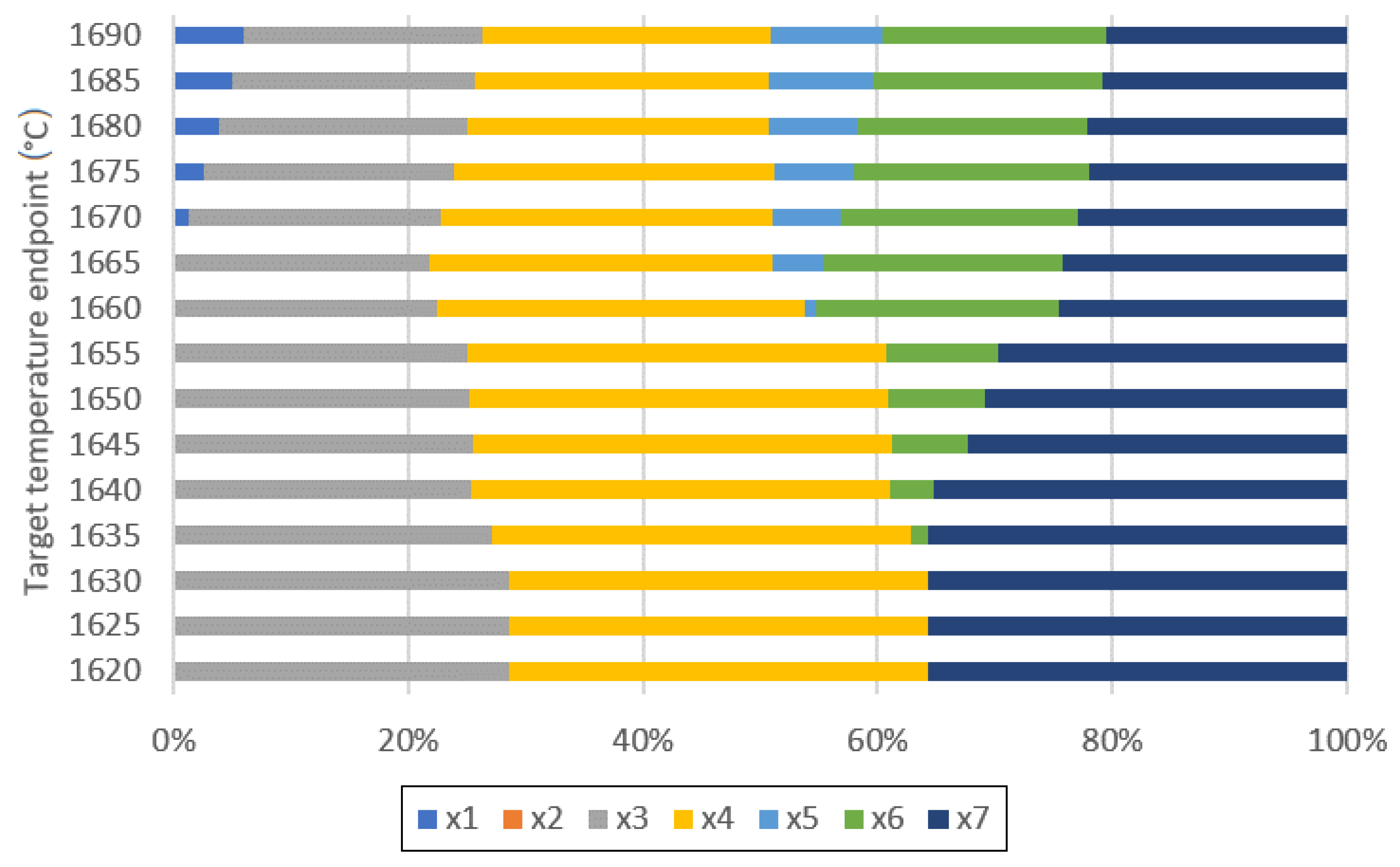
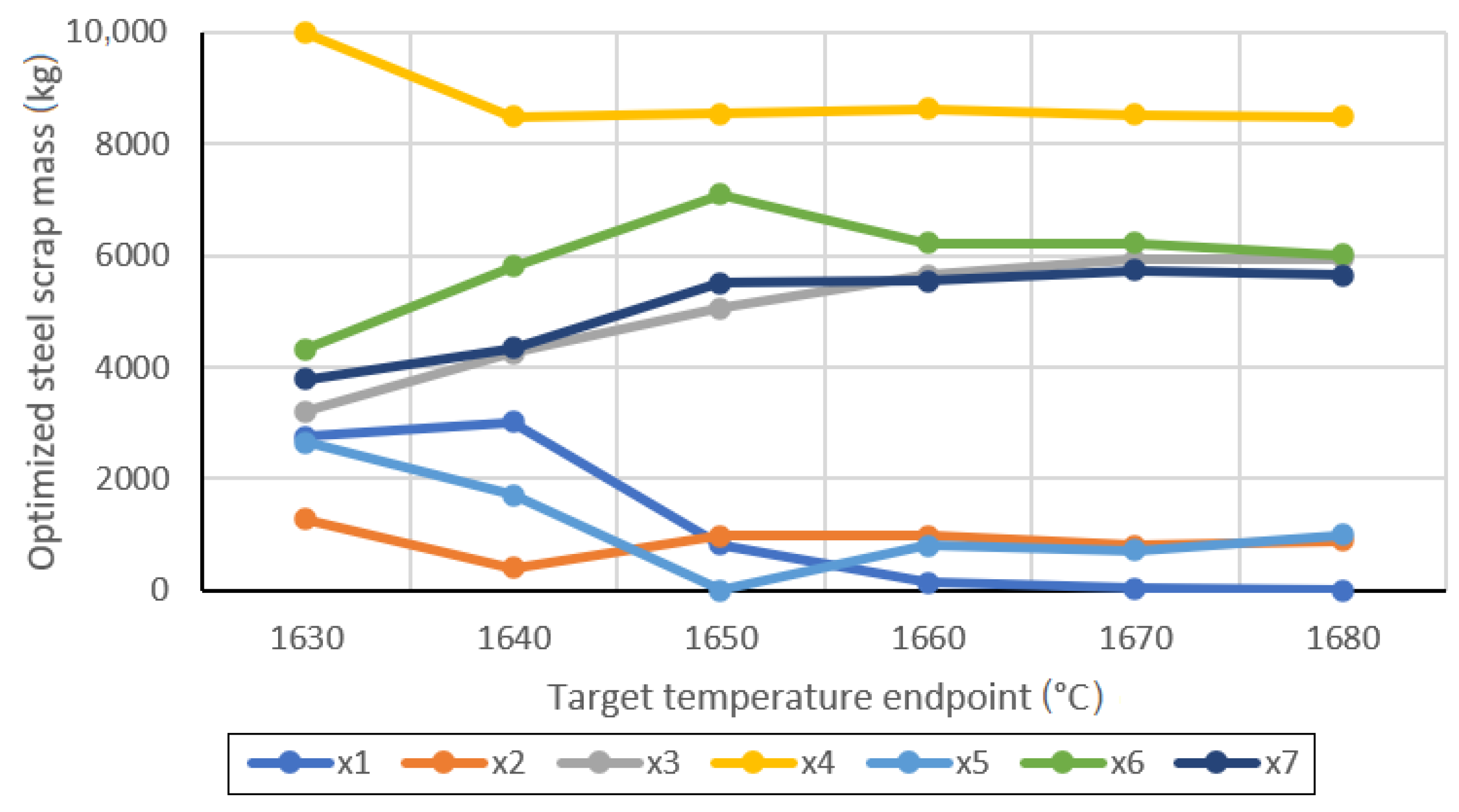
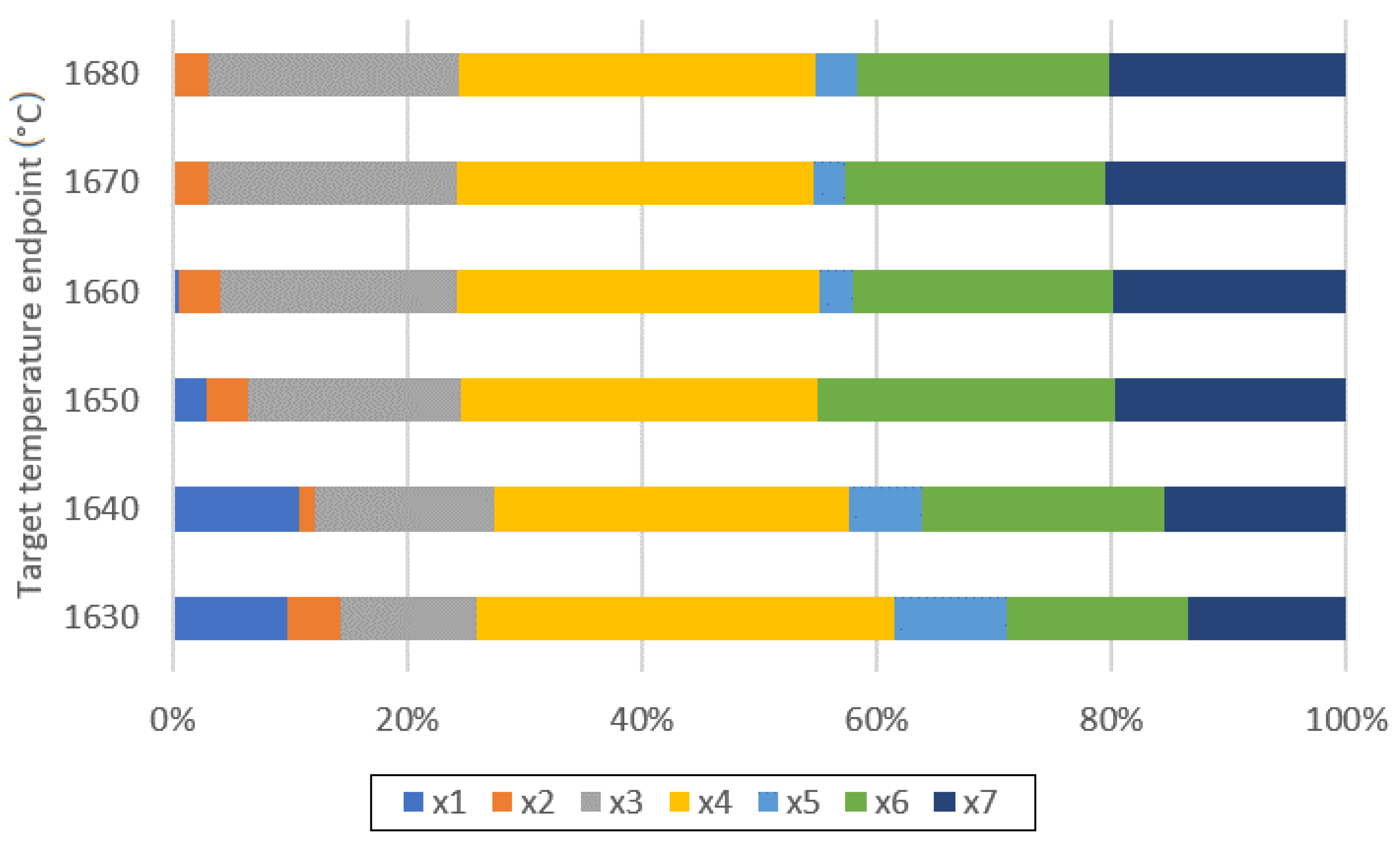
The optimized masses of individual scrap categories are shown in Figure 15. The stacked representation of the optimized percentage scrap distribution is shown in Figure 16.

The changes in the optimized distribution of individual scrap categories with increasing target temperature, particularly the pronounced redistribution observed around $T_{target}$ = 1660 °C, result from the nonlinear response represented by the GPR surrogate model together with the imposed mass-balance and variable-bound constraints. Although the decision variables $x_1$, …, $x_7$ represent different industrial scrap categories, their detailed metallurgical characteristics are not explicitly included as separate variables or constraints in the present optimization formulation. Therefore, the observed redistribution should not be interpreted as direct evidence of differences in scrap melting behavior. Rather, Figure 15 and Figure 16 show the scrap distributions preferred by the model for minimizing the predicted endpoint temperature error within the defined feasible region. A detailed metallurgical interpretation of these changes would require additional scrap-specific information and corresponding technological constraints.

The optimization algorithm identified a scrap composition that minimized the objective function under the imposed technological constraints. Optimization converged successfully for all investigated target temperatures. The optimization was performed using the trained GPR surrogate model rather than the original deterministic BOF model.

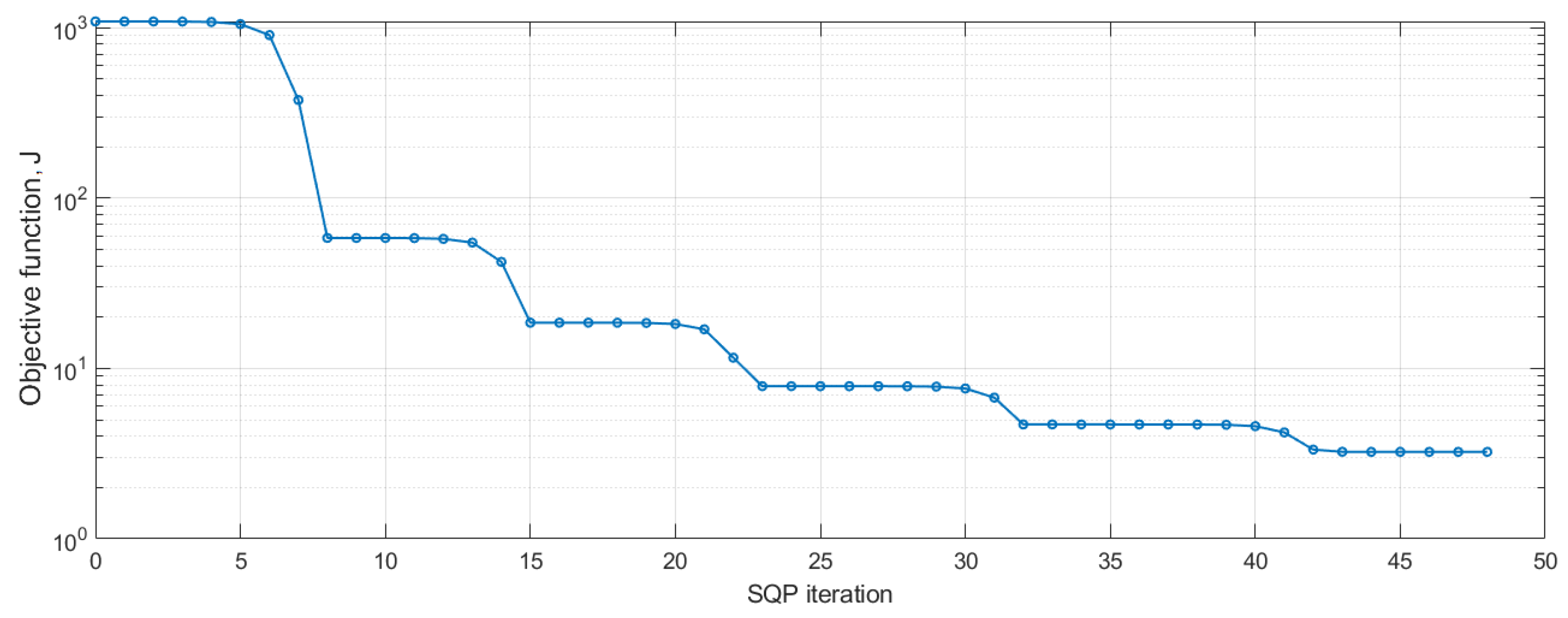
The convergence behavior of the GPR-based SQP optimization was additionally evaluated for all 15 target temperatures from 1620 °C to 1690 °C. All optimization runs terminated successfully. The number of SQP iterations ranged from 12 to 67, with a mean of 35.8 iterations, while the number of objective function evaluations ranged from 104 to 585 (mean 305.6). The measured optimization time ranged from approximately 0.10 to 1.35 s, with a mean of 0.41 s. For the representative case $T_{target}$ = 1650 °C, convergence was achieved after 48 iterations and 405 objective function evaluations. Figure 17 illustrates the corresponding decrease in the objective function value during the SQP iterations.

3.2.2. Optimization Using Deterministic Model

In this variant for optimizing the mass composition of steel scrap, a deterministic model of the BOF process was used within the optimization system with the model. The inputs to this model were real process data from ten melts.

The goal of the optimization was, as in the previous variant, to determine the optimal masses of individual scrap categories so that the assumed final temperature approaches the required target temperature and, at the same time, the technological mass-balance constraint (1) is met. The optimization algorithm of the gradient method was tested in the first step for the target final temperature $T_{target}$ = 1650 °C. The initial reference composition of the scrap was set to a constant value for all scrap types, namely 4000 kg.

Since it was a scrap optimization for a group of ten melts, the predicted final temperature was calculated as the average of the ten final temperatures obtained from the deterministic model. Using the reference composition of scrap, the deterministic model predicted the endpoint temperature as ${\widehat{T}}_{end, ref}$ = 1614.04 °C, which corresponds to a temperature deviation $e_{opt}$ = −35.96 °C. After optimization, the predicted endpoint temperature achieved by the deterministic model was ${\widehat{T}}_{end, ref}$ = 1623.35 °C, which corresponds to a final prediction error of $e_{opt}$ = −26.65 °C. The optimization procedure therefore reduced the temperature prediction error from 35.96 °C to 26.65 °C. Figure 18 shows the comparison between the reference and optimized scrap compositions obtained using optimization with the deterministic model.

In the subsequent evaluation of the optimization algorithm and the entire optimization system with the model, this procedure was repeated for several target end temperatures ranging from 1630 °C to 1680 °C in 10 °C increments for the same group of ten melts. For each target temperature, the same (constant) reference scrap composition was used as the starting point.

The numerical results are summarized in

Table 3. Multi-target optimization results using the deterministic model.

${\mathit{T}}_{\mathit{t}\mathit{a}\mathit{r}\mathit{g}\mathit{e}\mathit{t}}$ (°C)	${\widehat{\mathit{T}}}_{\mathit{r}\mathit{e}\mathit{f}}$ (°C)	${\mathit{e}}_{\mathit{r}\mathit{e}\mathit{f}}$ (°C)	${\widehat{\mathit{T}}}_{\mathit{o}\mathit{p}\mathit{t}}$ (°C)	${\mathit{e}}_{\mathit{o}\mathit{p}\mathit{t}}$ (°C)	Improvement (°C)
1630	1596.14	−33.86	1598.80	−31.20	2.66
1640	1603.47	−36.53	1609.97	−30.03	6.50
1650	1614.04	−35.96	1623.35	−26.65	9.31
1660	1619.62	−40.38	1633.42	−26.58	13.81
1670	1624.08	−45.92	1640.96	−29.04	16.88
1680	1627.45	−52.55	1645.53	−34.47	18.08

. The table compares the predicted endpoint temperature obtained using the reference scrap composition with the optimized prediction obtained after optimization.

As in the first optimization variant with the GPR surrogate model, in this case, the reference composition systematically underestimates the target final temperature over the entire investigated range. The optimized solution significantly shifts the predicted final temperature towards the target temperature. The absolute error of the reference composition increases from approximately 33.86 °C at $T_{target}$ = 1630 °C to 52.55 °C at $T_{target}$ = 1680 °C. After optimization, the absolute error over the entire range decreases compared to the reference error. This confirms that the optimization algorithm consistently improves the predicted end-point temperature for all investigated operating points.

The optimized masses of individual scrap categories are shown in Figure 19. The stacked representation of the optimized percentage scrap distribution is shown in Figure 20.

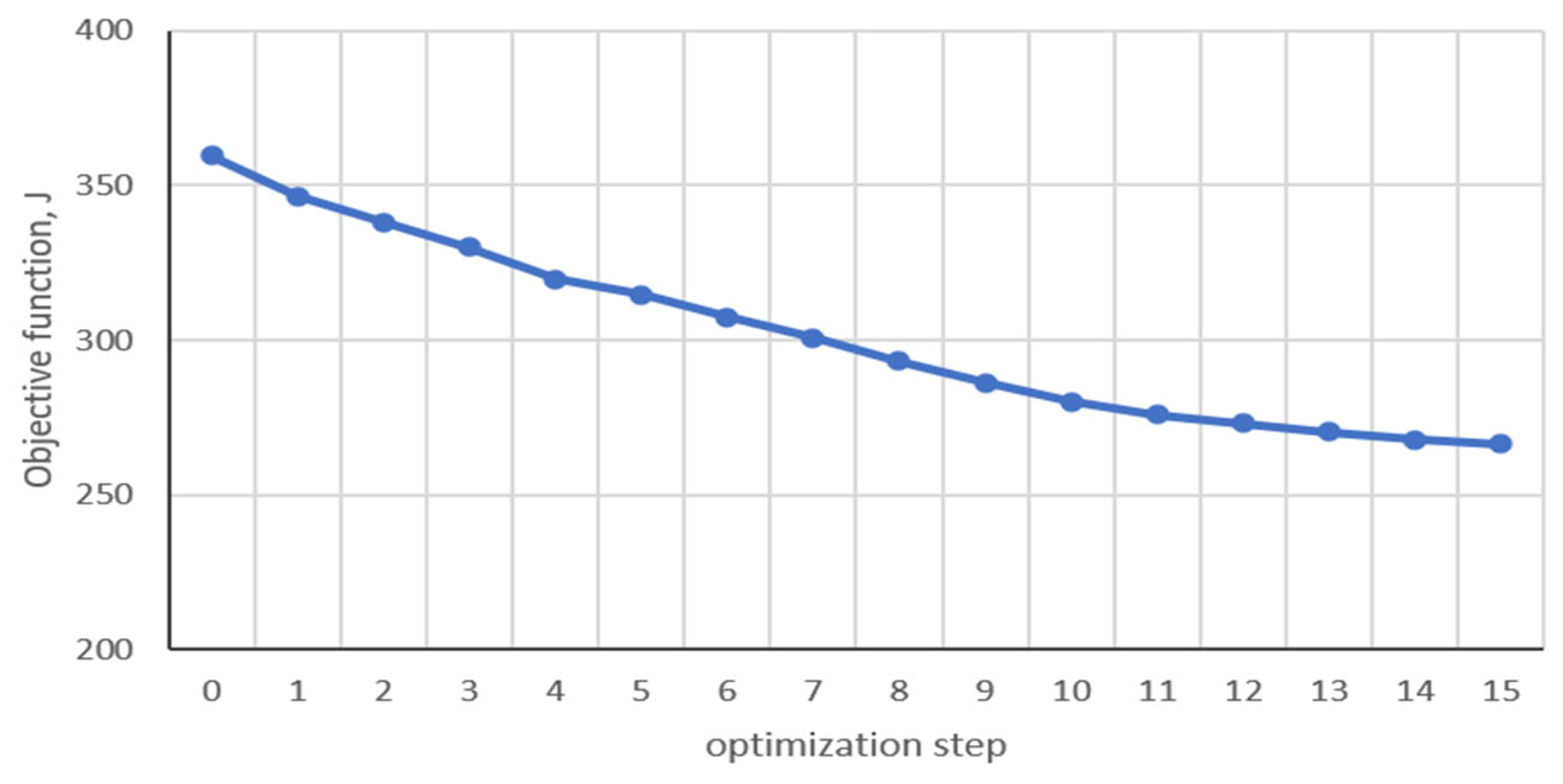
Since the optimization algorithm using the simulation model was only partially automated, it is not possible to determine the total optimization time unambiguously. The simulation time on the model for 10 melts was approximately 1 s. Eleven such simulations were required for one optimization step: ten partial ones for calculating the gradient components and one for the new components of the optimized vector. Thus, the simulation time for one optimization step was approximately 11 s. The optimization algorithm terminated based on the accuracy of the difference between the objective function values in the last two optimization steps. This accuracy was set to 0.5%. When the difference between the last two objective function values was less than the selected accuracy, the algorithm was terminated. The number of iterations (optimization steps) on the simulation model ranged from 12 to 20. For the representative case T_target = 1650 °C, the optimization terminated after 15 iterations. Figure 21 shows the corresponding decrease in the objective function value during the individual optimization steps for T_target = 1650 °C.

4. Discussion

The comparison of the investigated machine learning approaches showed that Gaussian Process Regression provided the highest prediction accuracy among the evaluated models. Although Support Vector Regression and Random Forest also produced acceptable results, GPR achieved the lowest prediction errors and the highest coefficient of determination, making it the most suitable surrogate model for the subsequent optimization task.

The obtained results indicate that the prediction accuracy of the GPR model was sufficient for its use within the investigated optimization framework. Since the optimization algorithm repeatedly evaluates the prediction model during the search process, replacing repeated evaluations of the detailed deterministic BOF process model with a computationally efficient surrogate can considerably simplify the optimization procedure. In addition to the surrogate-model optimization, the proposed methodology also investigated optimization using the original deterministic BOF model. While the deterministic model provides a more detailed process description, the machine learning surrogate provides a computationally simpler approximation that can be evaluated repeatedly during iterative optimization. Consequently, the proposed methodology offers two optimization strategies depending on the available process model and computational requirements.

Several optimization variants differing in the initial point and objective function formulation were investigated. The obtained optimized endpoint temperatures were practically identical, indicating that the optimization converged to the same solution regardless of initialization or the inclusion of the regularization term. This suggests that the identified optimum is robust within the investigated operating region.

The proposed methodology was evaluated using industrial data from a single BOF installation. An important limitation of the present study is that the machine learning surrogate models were trained to reproduce the outputs of the deterministic BOF model rather than directly measured industrial endpoint temperatures. Consequently, the reported MAE, RMSE, and $R^2$ values quantify surrogate-model agreement with the deterministic model and should not be interpreted as predictive accuracy against the actual BOF process. Any systematic error or uncertainty in the underlying deterministic model may therefore propagate through the surrogate model and subsequently affect the optimization results. Although the deterministic modeling approach has previously been validated against measured endpoint temperatures from industrial BOF heats, this validation does not replace direct validation of the present surrogate-based optimization framework. Future work should therefore validate the optimized solutions against measured endpoint temperatures and, when a sufficiently large industrial dataset becomes available, train and evaluate the surrogate models directly using measured plant data. A further limitation concerns the use of the prescribed target temperature as one of the surrogate-model inputs. Although this variable is distinct from the model-generated endpoint temperature used as the output, it represents a strong process-level predictor because the underlying deterministic BOF model itself incorporates the target temperature in its input structure. The resulting surrogate models should therefore not be interpreted as independent predictors of endpoint temperature based solely on physical charge characteristics. Rather, they approximate the input–output mapping of the underlying deterministic BOF process model for different scrap compositions and prescribed temperature targets. This dependence should be considered when interpreting the reported predictive performance and when transferring the methodology to other BOF operating conditions.

Figure 22 illustrates the overall framework of the proposed hybrid deterministic, regression, and machine learning methodology for BOF endpoint temperature prediction and scrap charge optimization.

The proposed methodology therefore combines metallurgical process knowledge, machine learning modeling, deterministic modeling, and nonlinear constrained optimization into a unified, optimization-oriented decision-support framework for BOF steelmaking.

The results show that both the developed GPR surrogate model and the complex deterministic model can be successfully integrated into constrained optimization frameworks for optimizing steel scrap in the BOF process. The optimization process reduced the predicted endpoint temperature deviation while satisfying the mass-balance and variable-bound constraints imposed in the present formulation. These results indicate that machine learning surrogate models can provide nonlinear approximations suitable for model-based optimization studies.

An important observation is that the optimization algorithm tended to drive several scrap variables toward their lower or upper bounds. Although these solutions satisfy the mathematical constraints imposed in the present formulation, they do not necessarily represent directly applicable industrial scrap recipes. In actual BOF operation, the admissible amount of each scrap category may additionally depend on scrap availability, cost, contractual requirements, chemical composition, and metallurgical restrictions, including limits associated with residual or tramp elements. Such plant-specific information was not available in the dataset used in this study; therefore, additional numerical constraints were not introduced without supporting operational data. As an additional sensitivity check, the optimization was also examined using different initial compositions and with or without a small regularization term penalizing deviations from the reference scrap composition. The investigated variants produced practically identical optimized solutions, indicating that, for the considered settings, the observed boundary solutions were not primarily caused by the choice of the initial point or by the absence of this weak regularization term. Consequently, practical implementation of the proposed framework would require the incorporation of plant-specific technological and operational constraints derived from actual production requirements. The obtained optimization results should be interpreted as model-based recommendations and not as directly validated industrial operating conditions. Nevertheless, the achieved reduction in the final temperature prediction error demonstrates the strong potential of combining machine learning models and nonlinear optimization, which can provide decision support for intelligent optimization.

Although the deterministic and surrogate-model optimization approaches are based on different mathematical models, both represent feasible methodologies for temperature-oriented scrap charge optimization. The deterministic model preserves the underlying metallurgical description of the process, whereas the surrogate approach provides a simplified approximation of the deterministic model while maintaining sufficient approximation accuracy for the investigated optimization task.

Comparison of This Work with Related Studies

Most recent BOF studies primarily focus on improving endpoint prediction accuracy using various machine learning techniques, including neural networks, support vector regression, ensemble learning, and deep learning. Although these approaches often achieve satisfactory prediction performance, the trained models are generally used only as predictive tools and are not incorporated into constrained optimization procedures for scrap charge design.

In contrast, several optimization-oriented studies formulate scrap selection as a cost, energy, or scheduling problem. However, endpoint temperature prediction is usually not directly integrated into the optimization loop.

The methodology proposed in this work differs from these approaches by combining three complementary components: (i) an existing deterministic BOF model, (ii) machine learning surrogate modeling, and (iii) nonlinear constrained optimization. The trained GPR model is used as a computationally efficient surrogate model that enables rapid evaluation of candidate scrap compositions during optimization.

To better position the proposed methodology within the current state of the art,

Table 4. Comparison of the proposed methodology with representative BOF endpoint prediction and optimization studies.

Study	ML Prediction	Scrap Optimization	Surrogate Model	Constrained Optimization
Jo et al. (2019) [4]	✓	-	-	-
Yang et al. (2023) [24]	✓	-	-	-
Wang et al. (2025) [25]	✓	-	-	-
Wang et al. (2012) [31]	-	✓	-	✓
Liu et al. (2026) [34]	✓	✓	✓	✓
Laciak et al. (2022) [22]	✓	-	✓	-
This work	✓	✓	✓ (GPR)	✓ (SQP/fmincon)

qualitatively compares representative studies on BOF endpoint prediction and scrap charge optimization. Rather than comparing prediction accuracy across different industrial datasets, the comparison focuses on the methodological characteristics of the individual approaches, including the use of machine learning, optimization techniques, surrogate modeling, and technological constraints.

As shown in Table 4, most published studies primarily address either endpoint prediction or scrap charge optimization as separate tasks. In contrast, the proposed methodology combines deterministic process modeling, machine learning surrogate modeling, and constrained nonlinear optimization within a unified framework. This enables surrogate-based temperature prediction and optimization-oriented decision support while maintaining computational efficiency suitable for repeated optimization.

The proposed surrogate models were trained using outputs of the existing deterministic-based BOF temperature model rather than directly measured industrial endpoint temperatures. Consequently, the obtained prediction accuracy reflects the approximation capability of the surrogate models with respect to the reference model. Future work will therefore focus on extending the methodology toward direct learning from industrial measurements and on incorporating additional process variables, including hot metal chemistry, oxygen consumption, and dynamic process information.

5. Conclusions

This paper presented a hybrid framework for endpoint temperature prediction and steel scrap charge optimization in basic oxygen furnace (BOF) steelmaking. The proposed methodology combines an existing deterministic BOF process model, regression modeling, machine learning surrogate models, and constrained nonlinear optimization. Two optimization strategies were investigated: optimization based on a machine learning surrogate model and direct optimization using the deterministic BOF process model.

Three machine learning approaches, namely Support Vector Regression (SVR), Random Forest Regression (RF), and Gaussian Process Regression (GPR), were implemented and evaluated using a dataset combining industrial operating inputs with endpoint temperatures generated by the deterministic BOF process model. Among the investigated machine learning models, GPR achieved the best approximation performance with respect to the reference deterministic-model outputs and was therefore selected as the surrogate model for subsequent optimization. The obtained results show that surrogate modeling can provide a computationally efficient approximation suitable for repeated evaluations within the optimization procedure.

The proposed optimization methodology enables the determination of scrap charge compositions satisfying the imposed mass-balance and variable-bound constraints while minimizing the deviation between the predicted and target endpoint temperatures. In addition to surrogate-model optimization, the study demonstrated that optimization can also be performed directly using the deterministic BOF process model. These complementary approaches provide flexibility depending on the available process model and computational requirements.

The present study was evaluated using operational records from 180 industrial BOF heats. However, the machine learning surrogate models were trained to reproduce endpoint temperatures generated by the deterministic BOF process model rather than directly measured industrial endpoint temperatures. Consequently, the reported prediction metrics quantify the agreement of the surrogate models with the reference deterministic model and should not be interpreted as direct predictive accuracy against the actual BOF process. Any systematic error or uncertainty in the deterministic model may therefore propagate through the surrogate model and subsequently affect the optimization results. The optimized scrap compositions should accordingly be interpreted as model-based recommendations rather than directly validated industrial operating conditions.

Future research will focus on extending the proposed framework by incorporating additional process variables affecting the BOF thermal state, investigating multi-objective optimization formulations involving production cost and energy consumption, and validating the surrogate-based optimization framework against directly measured industrial endpoint temperatures. Further work should also include plant-specific technological and operational constraints and validation using data from additional industrial installations. Another possible direction is the integration of the proposed optimization framework into industrial decision-support systems for scrap charge planning.

Overall, the proposed hybrid framework demonstrates the feasibility of combining deterministic process modeling, machine learning surrogate modeling, and constrained nonlinear optimization for model-based temperature-oriented scrap charge optimization in BOF steelmaking.

References

1. Slatosky, W.J. End-Point Temperature Control in LD Steelmaking. JOM 1960, 12, 226–230. [Google Scholar] [CrossRef] [Scilit]
2. Cai, B.-Y.; Zhao, H.; Yue, Y.-J. Research on the BOF steelmaking endpoint temperature prediction. In Proceedings of the 2011 International Conference on Mechatronic Science, Electric Engineering and Computer (MEC), Jilin, China, 19–22 August 2011; IEEE: New York, NY, USA, 2011; pp. 2278–2281. [Google Scholar] [CrossRef] [Scilit]
3. Duan, J.; Qu, Q.; Gao, C.; Chen, X. BOF steelmaking endpoint prediction based on FWATSVR. In Proceedings of the 2017 36th Chinese Control Conference (CCC), Dalian, China, 26–28 July 2017; IEEE: New York, NY, USA, 2017; pp. 4507–4511. [Google Scholar] [CrossRef] [Scilit]
4. Jo, H.; Hwang, H.J.; Phan, D.; Lee, Y.; Jang, H. Endpoint Temperature Prediction model for LD Converters Using Machine-Learning Techniques. In Proceedings of the 2019 IEEE 6th International Conference on Industrial Engineering and Applications (ICIEA), Tokyo, Japan, 12–15 April 2019; IEEE: New York, NY, USA, 2019; pp. 22–26. [Google Scholar] [CrossRef] [Scilit]
5. Kačur, J.; Flegner, P.; Durdán, M.; Laciak, M. Prediction of Temperature and Carbon Concentration in Oxygen Steelmaking by Machine Learning: A Comparative Study. Appl. Sci. 2022, 12, 7757. [Google Scholar] [CrossRef] [Scilit]
6. Dong, X.L.; Dong, S. The Converter Steelmaking End Point Prediction Model Based on RBF Neural Network. Appl. Mech. Mater. 2014, 577, 98–101. [Google Scholar] [CrossRef] [Scilit]
7. Qu, L.; Zhang, X.; Qu, Y. Research on BOF steelmaking endpoint control based on neural network. In Proceedings of the 2012 24th Chinese Control and Decision Conference (CCDC), Taiyuan, China, 23–25 May 2012; IEEE: New York, NY, USA, 2012; pp. 4110–4113. [Google Scholar] [CrossRef] [Scilit]
8. Fang, L.; Su, F.; Kang, Z.; Zhu, H. Artificial Neural Network Model for Temperature Prediction and Regulation during Molten Steel Transportation Process. Processes 2023, 11, 1629. [Google Scholar] [CrossRef] [Scilit]
9. Wei, Y.; Meng, H.J.; Huang, Y.J.; Xie, Z. Prediction on Molten Steel End Temperature during Tapping in BOF Based on LS-SVM and PSO. Adv. Mater. Res. 2012, 508, 233–236. [Google Scholar] [CrossRef] [Scilit]
10. Liang, B.; Wang, K.; Li, X. A Deep Learning Method for the Endpoint Carbon Prediction in BOF Steelmaking Process. In Proceedings of the 2024 IEEE 13th Data Driven Control and Learning Systems Conference (DDCLS), Kaifeng, China, 17–19 May 2024; IEEE: New York, NY, USA, 2024; pp. 666–671. [Google Scholar] [CrossRef] [Scilit]
11. Qiu, X.-F.; Zhang, R.-H.; Yang, J. Prediction of BOF endpoint carbon content and temperature via CSSA-BP neural network model. J. Iron Steel Res. Int. 2024, 32, 578–593. [Google Scholar] [CrossRef] [Scilit]
12. Cai, K.; Feng, K.; He, D.; Yang, L.; Zhang, M. Incorporation of Control Parameters into a Kinetic Model for Decarburization During Basic Oxygen Furnace (BOF) Steelmaking. Processes 2025, 13, 3048. [Google Scholar] [CrossRef] [Scilit]
13. Asai, S.; Muchi, I. Effect of Scrap Melting on the Process Variables in LD Converter Caused by the Change of Operating Conditions. Trans. Iron Steel Inst. Jpn. 1971, 11, 107–115. [Google Scholar] [CrossRef] [Scilit]
14. Asai, S.; Muchi, I. Effect of Scrap Melting on Temperature and Concentration of Carbon of Molten Steel in LD Converter. Tetsu-to-Hagane 1970, 56, 546–557. [Google Scholar] [CrossRef] [Scilit]
15. Asai, S.; Muchi, I. Theoretical Analysis of LD Converter Operation by Mathematical Model Considered Scrap-Melting Process. Tetsu-to-Hagane 1971, 57, 1331–1339. [Google Scholar] [CrossRef] [Scilit]
16. Kruskopf, A. A Model for Scrap Melting in Steel Converter. Metall. Mater. Trans. B 2015, 46, 1195–1206. [Google Scholar] [CrossRef] [Scilit]
17. Maunz, B.; Penz, F.M.; Schenk, J.; Bundschuh, P.; Panhofer, H.; Pastucha, K. Scrap Melting in BOF: Influence of Particle Surface and Size During Dynamic Converter Modeling. In Proceedings of the ABM Proceedings; Editora Blucher: São Paulo, Brazil, 2017; pp. 85–96. [Google Scholar] [CrossRef] [Scilit]
18. Wei, G.; Zhu, R.; Tang, T.; Dong, K. Study on the melting characteristics of steel scrap in molten steel. Ironmak. Steelmak. 2019, 46, 609–617. [Google Scholar] [CrossRef] [Scilit]
19. Xi, X.; Yang, S.; Li, J.; Chen, X.; Ye, M. Thermal simulation experiments on scrap melting in liquid steel. Ironmak. Steelmak. 2018, 47, 442–448. [Google Scholar] [CrossRef] [Scilit]
20. Xi, X.; Li, S.; Yang, S.; Zhao, M.; Li, J. Melting characteristics of steel scrap with different carbon contents in liquid steel. Ironmak. Steelmak. 2020, 47, 1087–1099. [Google Scholar] [CrossRef] [Scilit]
21. Singha, P. Scrap dissolution effect in BOF converter process. Ironmak. Steelmak. 2023, 50, 1434–1442. [Google Scholar] [CrossRef] [Scilit]
22. Laciak, M.; Kačur, J.; Terpák, J.; Durdán, M.; Flegner, P. Comparison of Different Approaches to the Creation of a Mathematical Model of Melt Temperature in an LD Converter. Processes 2022, 10, 1378. [Google Scholar] [CrossRef] [Scilit]
23. Liu, Z.; Liu, H.; Chen, F.; Li, H.; Xue, X. Dynamic Soft Sensor Model for Endpoint Carbon Content and Temperature in BOF Steelmaking Based on Adaptive Feature Matching Variational Autoencoder. Processes 2024, 12, 1807. [Google Scholar] [CrossRef] [Scilit]
24. Yang, L.; Liu, H.; Chen, F. Soft sensor method of multimode BOF steelmaking endpoint carbon content and temperature based on vMF-WSAE dynamic deep learning. High Temp. Mater. Process. 2023, 42, 20220270. [Google Scholar] [CrossRef] [Scilit]
25. Wang, H.; Liu, H.; Chen, F.; Li, H.; Xue, X. Endpoint carbon content and temperature prediction model in BOF steelmaking based on posterior probability and intra-cluster feature weight online dynamic feature selection. High Temp. Mater. Process. 2025, 44, 20240067. [Google Scholar] [CrossRef] [Scilit]
26. Yang, Y.; Chen, W.; Wei, L.; Chen, X. Robust optimization for integrated scrap steel charge considering uncertain metal elements concentrations and production scheduling under time-of-use electricity tariff. J. Clean. Prod. 2018, 176, 800–812. [Google Scholar] [CrossRef] [Scilit]
27. Schmidt, C. Distributionally Robust Optimization for Scrap Blending in EAF Steelmaking. In Proceedings of the 2025 IEEE International Conference on Technology Management, Operations and Decisions (ICTMOD), Glasgow, UK, 20–22 October 2025; IEEE: New York, NY, USA, 2025; pp. 1–6. [Google Scholar] [CrossRef] [Scilit]
28. Wang, H.-B.; Xu, A.-J.; Ai, L.-X.; Tian, N.-Y. Prediction of Endpoint Phosphorus Content of Molten Steel in BOF Using Weighted K-Means and GMDH Neural Network. J. Iron Steel Res. Int. 2012, 19, 11–16. [Google Scholar] [CrossRef] [Scilit]
29. Wang, X.; Xing, J.; Dong, J.; Wang, Z. Data driven based endpoint carbon content real time prediction for BOF steelmaking. In Proceedings of the 2017 36th Chinese Control Conference (CCC), Dalian, China, 26–28 July 2017; IEEE: New York, NY, USA, 2017; pp. 9708–9713. [Google Scholar] [CrossRef] [Scilit]
30. Zhou, M.; Zhao, Q.; Chen, Y. Endpoint prediction of BOF by flame spectrum and furnace mouth image based on fuzzy support vector machine. Optik 2019, 178, 575–581. [Google Scholar] [CrossRef] [Scilit]
31. Wang, C.; Bramming, M.; Larsson, M. Numerical Model of Scrap Blending in BOF with Simultaneous Consideration of Steel Quality, Production Cost, and Energy Use. Steel Res. Int. 2012, 84, 387–394. [Google Scholar] [CrossRef] [Scilit]
32. Vuleta, M.; Žugić, M.; Andrejić, V.; Ristić, T. Industrial optimization of BOF steelmaking: Increasing scrap ratio through hot metal parametar control. In Proceedings of the 56th International October Conference on Mining and Metallurgy—Zbornik Radova; University of Belgrade—Technical Faculty in Bor: Belgrade, Serbia, 2025; pp. 300–303. [Google Scholar] [CrossRef] [Scilit]
33. Manerba, D.; Mansini, R.; Tomasetti, L.; Zanotti, R. Bi-Objective Optimization in Steelmaking: Balancing Scrap Costs, Energy Consumption, and Steel Quality. IFAC-PapersOnLine 2025, 59, 1706–1711. [Google Scholar] [CrossRef] [Scilit]
34. Liu, Z.; Yan, L.; Han, X.; Qi, X.; Shi, S.; Li, B. Development and Application of a Hybrid Mechanistic-AI Model for Flux Optimization in High-Scrap-Ratio Converter Steelmaking of High-Manganese Steel for LNG Tanks. Metall. Mater. Trans. B 2026, 57, 4145–4161. [Google Scholar] [CrossRef] [Scilit]
35. Mahanta, B.K.; Gupta, P.; Mohanty, I.; Roy, T.K.; Chakraborti, N. Evolutionary data driven modeling and tri-objective optimization for noisy BOF steel making data. Digit. Chem. Eng. 2023, 7, 100094. [Google Scholar] [CrossRef] [Scilit]
36. Madhavan, N.; Brooks, G.; Overbosch, A.; Rhamdhani, M.; Rout, B. Potential for Increased Scrap Melting in a BOF. In Proceedings of the AISTech 2022 Proceedings of the Iron and Steel Technology Conference, Pittsburgh, PA, USA, 16–18 May 2022; AIST: Sydney, Australia, 2022; pp. 441–449. [Google Scholar] [CrossRef] [Scilit]
37. Kurth, H.; Kalicinski, M. Real-Time On-Line Elemental Analysis of Scrap for Steelmaking. In Proceedings of the AISTech 2023 Proceedings, Detroit, MI, USA, 8–11 May 2023; AIST: Sydney, Australia, 2023. [Google Scholar] [CrossRef] [Scilit]
38. Schafer, M.; Faltings, U.; Glaser, B. Machine learning approach for predicting tramp elements in the basic oxygen furnace based on the compiled steel scrap mix. Sci. Rep. 2025, 15, 2430. [Google Scholar] [CrossRef] [Scilit]
39. Smirnov, N.V.; Rybin, E.I. Machine Learning Methods for Solving Scrap Metal Classification Task. In Proceedings of the 2020 International Russian Automation Conference (RusAutoCon), Sochi, Russia, 6–12 September 2020; IEEE: New York, NY, USA, 2020; pp. 1020–1024. [Google Scholar] [CrossRef] [Scilit]
40. Yin, J.; Xiao, P.; Zhang, B.; Zhu, L. Scrap weight prediction for different scrap types based on semantic segmentation and machine learning. Mach. Vis. Appl. 2026, 40, 104. [Google Scholar] [CrossRef] [Scilit]
41. Laciak, M.; Kačur, J.; Durdán, M.; Flegner, P. System of indirect measurement temperature of melt with adaptation module. In Proceedings of the 16th International Carpathian Control Conference (ICCC), Szilvasvarad, Hungary, 27–30 May 2015; IEEE: New York, NY, USA, 2015; pp. 277–281. Available online: https://ieeexplore.ieee.org/document/7145088 (accessed on 25 May 2026).
42. Laciak, M.; Kačur, J.; Flegner, P.; Durdán, M.; Pavlíčková, M.; Terpák, J. The Analysis of the Influence of Input Parameters on the Accuracy of Temperature Model in the Steelmaking Process. In Proceedings of the 23rd International Carpathian Control Conference (ICCC), Sinaia, Romania, 29 May–1 June 2022; IEEE: New York, NY, USA, 2022; pp. 366–369. Available online: https://ieeexplore.ieee.org/document/9805906 (accessed on 25 May 2026).
43. Smola, A.J.; Schölkopf, B. A tutorial on support vector regression. Stat. Comput. 2004, 14, 199–222. [Google Scholar] [CrossRef] [Scilit]
44. Vapnik, V.; Golowich, S.; Smola, A.J. Support vector method for function approximation, regression estimation and signal processing. In Advances in Neural Information Processing Systems; MIT Press: Cambridge, MA, USA, 1997. [Google Scholar]
45. Hastie, T.; Tibshirani, R.; Friedman, J. The Elements of Statistical Learning, 2nd ed.; Springer: Berlin/Heidelberg, Germany, 2009. [Google Scholar]
46. Breiman, L. Random Forests. Mach. Learn. 2001, 45, 5–32. [Google Scholar] [CrossRef] [Scilit]
47. Rasmussen, C.E.; Williams, C.H.K. Gaussian Processes for Machine Learning; MIT Press: Cambridge, MA, USA, 2006. [Google Scholar]
48. Laciak, M.; Kačur, J.; Flegner, P.; Durdán, M.; Pavlíčková, M.; Terpák, J. Use of the optimization system with a model for optimizing parameters of technological processes. In Proceedings of the 25th International Carpathian Control Conference (ICCC), Krynica Zdrój, Poland, 22–24 May 2024; IEEE: New York, NY, USA, 2024; pp. 1–5. Available online: https://ieeexplore.ieee.org/document/10569965 (accessed on 25 May 2026).
Figure 1. Conceptual overview of the proposed intelligent BOF steelmaking framework combining machine learning surrogate modeling and constrained optimization for scrap charge optimization and endpoint temperature prediction.
Processes 14 02719 g001
Figure 2. Principal scheme of the deterministic model.
Processes 14 02719 g002
Figure 4. Complete dataset outputs used for model development.
Processes 14 02719 g004
Figure 5. Complete dataset inputs used for model development: (a) scrap mass x 1 (kg), (b) scrap mass x 2 (kg), (c) scrap mass x 3 (kg), (d) scrap mass x 4 (kg), (e) scrap mass x 5 (kg), (f) scrap mass x 6 (kg), (g) scrap mass x 7 (kg), and (h) target temperature x 8 = T t a r g e t   (°C).
Processes 14 02719 g005
Figure 6. Regression model prediction performance for the training dataset.
Processes 14 02719 g006
Figure 7. Regression model prediction performance for the testing dataset.
Processes 14 02719 g007
Figure 8. SVR prediction performance for the training dataset.
Processes 14 02719 g008
Figure 9. SVR prediction performance for the testing dataset.
Processes 14 02719 g009
Figure 10. RF prediction performance for the training dataset.
Processes 14 02719 g010
Figure 11. RF prediction performance for the testing dataset.
Processes 14 02719 g011
Figure 12. GPR prediction performance for the training dataset.
Processes 14 02719 g012
Figure 13. GPR prediction performance for the testing dataset.
Processes 14 02719 g013
Figure 14. Comparison of the reference and optimized scrap compositions obtained using the GPR surrogate model ( T t a r g e t = 1650 °C).
Processes 14 02719 g014
Figure 15. Optimized scrap composition for different target endpoint temperatures.
Processes 14 02719 g015
Figure 16. Stacked optimized percentage scrap composition for different target endpoint temperatures.
Processes 14 02719 g016
Figure 17. Convergence of the GPR surrogate-based SQP optimization for T t a r g e t = 1650 °C.
Processes 14 02719 g017
Figure 18. Comparison of the reference and optimized scrap compositions obtained using the deterministic model ( T t a r g e t = 1650 °C).
Processes 14 02719 g018
Figure 19. Optimized scrap composition for different target endpoint temperatures (using the deterministic model).
Processes 14 02719 g019
Figure 20. Stacked optimized percentage scrap composition for different target endpoint temperatures (using the deterministic model).
Processes 14 02719 g020
Figure 21. Convergence of the objective function for optimization with the deterministic model for T t a r g e t = 1650 °C.
Processes 14 02719 g021
Figure 22. Overall framework of the proposed hybrid deterministic, regression, and machine learning methodology for BOF steelmaking ( x 1 , …,   x 7 —masses of scrap in categories; T t a r g e t —target endpoint temperature; and T ^ e n d —predicted endpoint temperature).
Processes 14 02719 g022