


Abstract
Effective task allocation is fundamental to the success of heterogeneous multi-robot cooperative missions in smart manufacturing workshops, yet real-world operational uncertainties pose severe challenges to solution feasibility and mission robustness. Addressing these challenges, this paper focuses on the inspection and maintenance task allocation problem for heterogeneous mobile robot teams operating under fluctuating equipment maintenance time windows, variable task execution durations, and uncertain robot travel speeds caused by workshop congestion and payload variations. First, the aforementioned uncertain parameters are characterized using triangular fuzzy numbers, upon which a fuzzy chance-constrained programming model is constructed with the objective of minimizing total operational cost while ensuring constraint satisfaction under uncertainty. The proposed model simultaneously handles two types of critical constraints: the service time window constraint, which requires each task to be completed before its latest allowable service deadline, and the time sequence constraint, which enforces that each equipment inspection task must be completed prior to the corresponding maintenance task. Then, to tackle the inherent NP-hardness of this problem, a multi-strategy hybrid Harris Hawks Optimization algorithm incorporating differential evolution, termed MSHHODE, is proposed. In detail, three targeted enhancement mechanisms are introduced: a hunting enthusiasm factor that governs the dynamic balance between global exploration and local exploitation throughout the search process; an elite-assisted guidance strategy that stabilizes convergence by leveraging high-quality solutions to direct population evolution; and an adaptive differential evolution mechanism that reinforces global search diversity and mitigates premature convergence to local optima. Finally, simulation experiments conducted across multiple workshop-scale scenarios demonstrate that MSHHODE consistently outperforms benchmark algorithms across different key performance metrics under varied uncertain conditions, which validates the effectiveness and robustness of the proposed approach in solving complex, constrained allocation problems, offering a practical and reliable framework for real-world heterogeneous multi-robot task planning in smart manufacturing environments.
1. Introduction
In recent years, the rapid development of smart manufacturing technology has brought tremendous benefits to modern industrial production due to its advantages of high efficiency, flexibility, and reduced labor dependency [1,2]. At the same time, the collaboration among multiple mobile robots can further enhance the capability of a single robot, enabling multi-robot systems to complete more complex tasks with higher efficiency, quality, and robustness [3,4,5]. It is noted that the core challenges of multi-robot cooperation, such as task allocation, path planning, and motion planning, play a decisive role in the execution of manufacturing missions and have received widespread attention [6,7,8].
Among them, task allocation refers to assigning a set of tasks to each robot with all constraints satisfied and optimizing a specific objective function to maximize overall operational benefits [9,10]. In smart manufacturing workshops, mobile robots are typically required to perform two sequential operations on target equipment: an inspection task (e.g., fault diagnosis, quality detection) followed by a maintenance task (e.g., repair, lubrication, component replacement), where the maintenance operation can only be initiated after the corresponding inspection is completed. However, when multiple heterogeneous robots perform tasks in actual workshop environments, various uncertain factors arise inevitably, including unknown fault complexity leading to uncertain task execution durations, dynamic production schedule adjustments causing fluctuating maintenance time windows, and workshop congestion or varying payloads resulting in uncertain robot travel speeds [11,12,13]. These uncertain factors impose more stringent requirements on the coordination of multi-robot systems [14]. However, most existing studies are based on static and deterministic task environments, often neglecting the instability of various factors in the workshop, such as the uncertainty of equipment maintenance duration and the impact of floor traffic conditions on robot traveling speed [15]. This leads to task allocation schemes optimized under predetermined deterministic conditions often failing to achieve the expected results in actual execution, or even causing equipment to exceed its maintenance deadline, resulting in unplanned production line interruptions [16].
Therefore, how to pre-consider the impact of uncertainties on the allocation results of heterogeneous multi-robot tasks, thereby improving the robustness of the allocation scheme, has become an unavoidable key issue in the practical deployment of multi-robot systems in smart manufacturing [17]. By predicting and handling various uncertainties during the pre-allocation phase, a stable task allocation scheme that is insensitive to uncertainty interference can be generated, which effectively reduces the impact of disturbances and minimizes the need for real-time rescheduling during task execution.
To address the aforementioned challenges, this paper investigates the heterogeneous multi-robot task allocation problem in smart manufacturing workshops under uncertain operational conditions, including stochastic task execution durations, fluctuating maintenance time windows, and uncertain robot travel speeds, subject to multiple complex mission constraints, including temporal sequencing and time window requirements. The main contributions of this work are summarized as follows.
(1) A fuzzy chance-constrained programming model is constructed based on fuzzy reliability theory, with the objective of minimizing total operational cost. By characterizing uncertain parameters through triangular fuzzy numbers and their associated membership functions, the proposed model circumvents the need for pre-estimation of probability distribution laws, which offers greater modeling flexibility and applicability under data-scarce conditions.
(2) To efficiently solve this NP-hard combinatorial optimization problem, a Multi-Strategy Hybrid Harris Hawks Optimization (HHO) algorithm integrated with Differential Evolution (MSHHODE) is proposed. Three synergistic enhancement mechanisms are embedded into the standard HHO framework: a hunting enthusiasm factor that adaptively regulates the transition between global exploration and local exploitation; an elite-assisted guidance strategy that leverages superior solutions to stabilize population convergence; and an adaptive differential evolution mechanism that broadens search diversity and suppresses premature convergence to local optima.
(3) Comprehensive simulation experiments are conducted across multiple test scenarios, with systematic comparisons against representative benchmark algorithms. The results substantiate the effectiveness, robustness, and competitive superiority of the proposed MSHHODE in solving complex, constrained heterogeneous multi-robot task allocation problems under uncertainty.
The rest of this paper is organized as follows. Section 2 discusses the related work on task allocation for multiple robots under uncertainty. Section 3 formulates the considered multi-robot task allocation problem mathematically. The main structure of MSHHODE is illustrated in Section 4. Several simulations and comparisons are conducted in Section 5 to demonstrate the performance of MSHHODE. Section 6 concludes this paper.
2. Related Work
2.1. Smart Manufacturing Technology
With the development of technologies such as industrial Internet of Things, artificial intelligence, and digital twins, the manufacturing industry is shifting from a traditional scale efficiency orientation to a new paradigm of intelligence, flexibility, and service. Ref. [18] discussed the key technologies driving intelligent manufacturing and emphasized the progress of manufacturing technology that provides unprecedented design freedom. For modeling and simulation in a flexible manufacturing system (FMS), ref. [19] described the use of dedicated analysis and simulation software, through which the structure of the system can be established and specific technical and economic parameters can be determined for each processing and transport capacity. Different processing scenarios will be evaluated through virtual modeling and simulations in order to improve the performance and efficiency of the system. Ref. [20] demonstrated a practical implementation of a smart manufacturing application using a systematic approach based on a conceptual six-gear smart factory roadmap with connectivity, integration, and analytics stages to build a smart production management ecosystem using off-the-shelf technologies applied in precision manufacturing.
In addition, the AI approach to building flexible manufacturing systems has also been explosively researched [21,22]. In [23], the framework of the situation–actors–process (SAP) and learning–actions–performance (LAP) dimensions for the effective implementation of Gen AI is used to empower FMS. Ref. [24] provided a comprehensive overview of the current state of explainable AI, with a particular focus on recent advances and its critical role in enhancing trust and transparency in AI-driven smart manufacturing systems. Ref. [25] proposed the concept of human-centric smart manufacturing to entail a symbiotic human–machine relationship, and Trustworthy AI has been systematically reviewed as a key enabler through a progressive framework that addresses safety, transparency, and participatory updating across the product lifecycle.
Furthermore, the uncertainties within manufacturing systems are also gaining more and more attention. Ref. [26] combined generalized nets and intuitionistic fuzzy pairs, as measures of the uncertainty, for the modeling of flexible manufacturing systems and for the construction of simulation models. To address the uncertainties in the supply chain, ref. [27] proposed a hybrid fuzzy genetic algorithm framework that overcomes these constraints by combining the interpretability of fuzzy logic with the global search efficiency of genetic algorithms. Ref. [14] proposed a digital twin framework based on deep reinforcement learning for rapid response and system interaction to the uncertainty of corresponding demands and production dynamics. This framework provides fast and adaptive virtual reality interaction and dynamic batch publishing strategies, while reducing production costs and improving the satisfaction rate of production dynamics.
Overall, current research on smart manufacturing has made positive progress in system modeling, AI empowerment, and uncertainty response, with increasingly diverse technological paths. However, the cross-scenario universality of each method and its effectiveness in handling uncertain parameters in each scenario still need further verification.
2.2. Handling Parameter Uncertainty
Uncertainty is a major characteristic of realistic smart manufacturing workshop environments, making the study of heterogeneous multi-robot task allocation under uncertain conditions of great significance for practical industrial deployment. In workshop settings, uncertainty arises from multiple sources, including unpredictable equipment fault complexity, dynamically adjusted production schedules, and fluctuating robot travel speeds caused by congestion and varying payload conditions. These uncertainties directly affect the feasibility and optimality of pre-planned task allocation schemes, potentially leading to missed maintenance deadlines and unplanned production disruptions. Currently, most multi-robot task allocation studies are based on deterministic environments and cannot adequately handle the impact of such uncertainties on allocation schemes. Typically, uncertain parameters are incorporated into the optimization model as random variables or imprecise quantities. Depending on how these uncertain parameters are described and processed, there are three main approaches to addressing the impact of uncertain factors on task allocation: stochastic programming, robust optimization, and fuzzy programming.
Stochastic programming, as a commonly used method for dealing with uncertainty, introduces uncertain random variables described by probability distribution functions, and solves them by establishing a random-variable model of the optimization objective function [28]. Ref. [29] proposed a two-stage stochastic 0-1 integer linear programming model to equitably optimize ambulance allocation in the Basque Country, balancing multi-interval response times between urban and rural areas through stochastic programming. Ref. [30] developed a two-stage stochastic optimization model that jointly allocates Emergency Mobility Facilities (EMFs) and designed road networks for disaster response, addressing uncertainties in demand and congestion through reformulation into a tractable mixed-integer linear program validated with real-world data. However, the application of stochastic programming methods requires estimating the distribution of uncertain parameters, and the estimated distribution needs to be close enough to the actual distribution. In actual environments, though, it is difficult to obtain the probability of uncertain events [31].
Therefore, some scholars have used robust optimization methods to solve the optimization problem under uncertain conditions. By controlling the conservative parameters of decision-making, the uncertain optimization model is transformed into a deterministic linear programming model [32]. Since there is no need to assume the distribution of uncertain parameters, it is easier to solve than the stochastic programming model. Ref. [33] proposed a multi-objective mathematical model based on multi-scenario robust optimization for the optimal design and facility location allocation of blood supply chain networks after natural disasters, aiming to minimize shortages and costs. Ref. [34] proposed a two-stage robust optimization model integrating prospect theory for the berth allocation and quay crane assignment problem under uncertainty, along with an accelerated algorithm for efficient large-scale solutions. Ref. [35] proposed a scenario-based robust optimization model for sustainable distributed flow-shop scheduling under uncertainty, solved by an Adaptive Large Neighborhood Search algorithm to enhance energy efficiency, job creation, and workday utilization. However, the task allocation schemes solved by robust optimization methods are often overly conservative, making it difficult to balance system performance and protection against uncertainty.
In addition to the two methods mentioned above, the fuzzy programming method describes the uncertain parameters in the form of fuzzy sets also widely applied to solve task allocation problems under uncertain conditions. It only needs to select the membership function of the uncertain variables based on prior knowledge and emphasizes the possibility of satisfying the constraints [36]. By transforming the objective function and constraints of the fuzzy programming into a general form of a programming model, the fuzzy optimal solution can be obtained. Ref. [37] proposed a Stackelberg game-based fuzzy optimization model for tugboat scheduling under uncertainty, solved by an enhanced seagull algorithm and validated with real port data. Ref. [38] developed a fuzzy multi-constraint programming model and a dynamic strategy with an enhanced grey wolf optimization algorithm for heterogeneous multi-robot dynamic task assignment under uncertainty, demonstrating 5–30% performance improvement. The fuzzy programming technique with a linear membership function is applied in [39] to generate efficient and non-dominated allocations with better optimal values and degrees of satisfaction of objective functions for different values of parameters and for fuzzy preferences. Ref. [40] developed a fuzzy multi-criteria decision-making model for resilient supplier selection under dynamic conditions, optimized by an enhanced wolf pack algorithm for order allocation, and validated its feasibility through a case study in the new energy vehicle industry.
The above three types of methods focus on how to make optimal decisions under uncertainty, but in addition to making reasonable decision plans, it is also necessary to quantitatively evaluate the reliability of existing plans. Fuzzy reliability theory, on the other hand, focuses on how reliable the design scheme is, which means the ability of the system to complete the specified functions under specified conditions and within a specified time [41]. This theory introduces fuzzy sets into traditional reliability engineering to address the problem of difficulty in obtaining accurate failure probabilities.
At the methodological level, fuzzy reliability is mainly achieved through fuzzy fault tree analysis. Firstly, for example, the failure probability of basic events is represented by fuzzy numbers, such as triangular fuzzy numbers, and then the fuzzy failure probability and fuzzy reliability of the top event are calculated. Ref. [42] investigated the mixed statistical fuzzy reliability evaluation composed of intuitionistic fuzzy sets (IFSs) and interval-valued intuitionistic fuzzy sets. In [43], a fault tree analysis based on the fuzzy set theory is presented and applied to a wind energy system. The fault probabilities are regarded as a fuzzy number, the fuzzy failure rate is known by using fuzzy rules, and the risk analysis method is applied based on the fuzzy risk index (FRI) to know the exact impact of every basic event on the top event.
In addition, the stress strength fuzzy interference model and the combination method of fuzzy fault tree with Bayesian network and Petri net have also been applied in the reliability evaluation of complex manufacturing systems. For example, ref. [44] proposed a reliability analysis method based on fuzzy polymorphic Bayesian network (FPBN), which utilizes a multi-state fault tree to construct a polymorphic Bayesian network (BN), combining traditional BN techniques with a consideration of multiple fault states and fuzzy failure rates to handle inaccurate fault data and unclear logical relationships. Ref. [45] combined fuzzy BN with result simulation, using leakage noise or gate, intuitionistic fuzzy set theory, and similarity aggregation for expert inspiration to fill the conditional probability table, and used Safeti software for result analysis.
2.3. Recent Developments of Harris Hawks Optimization
Since its proposal by Heidari et al. in 2019, the HHO algorithm has rapidly become a research hotspot in the field of swarm intelligence optimization due to its unique mechanism of simulating Harris hawk cooperative hunting behavior and the advantage of not requiring gradient information [46,47]. However, standard HHO still faces inherent limitations such as slow convergence speed, insufficient population diversity, and susceptibility to falling into local optima in high-dimensional complex problems.
To overcome the above shortcomings, researchers have continuously improved HHO from multiple dimensions such as parameter control, strategy improvement, and hybrid enhancement, and have derived a large number of variant algorithms. For example, ref. [48] integrated an improved HHO (IIHHO) algorithm, which introduces an intermittent energy regulator, a regularized vector mechanism, a refined Lévy flight search scope, and a Cardano formula-based step-size adjustment to collectively enhance local search capability, escape from local optima, and increase solution accuracy. Ref. [49] improved Harris Hawks optimization (IHHO) by modifying the exploration phase with random location-based habitats and refining exploitation via three strategies, while employing logarithm- and exponential-based random value generation to escape local optima, demonstrating superior performance across diverse benchmarks and engineering problems. The proposed Chaotic Harris Hawks Optimization (CHHO) in [50] enhances the standard HHO by introducing chaotic maps at the initialization phase to improve population diversity and incorporating simulated annealing on the current best solution to strengthen exploitation, thereby addressing the local optima and diversity limitations for feature selection problems. Ref. [51] applied chaotic maps at the initialization phase of HHO to enhance the population diversity in the search space, and used the simulated annealing (SA) algorithm to the current best solution to improve HHO exploitation. Ref. [52] proposed a Modified HHO (MHHO) that integrates Leader-Guided Perching (LGP) to accelerate movement toward promising regions, an Adaptive Deception Factor (ADF) to dynamically scale Lévy-flight intensity to escape deceptive local optima, and a Hierarchical Attack Strategy (HAS) to replaces the hard besiege phase with a mentor-guided exploitation step to mitigate swarm clumping and refine local search. The comparison table of the HHO algorithm literature is shown in Table 1.
Table 1.
Feature comparison of representative HHO variants and the proposed MSHHODE.
As shown in Table 1, existing HHO variants typically improve only a single stage of the search process and retain the fixed energy-threshold switching criterion, with any guidance mechanisms applied to a single individual rather than the population. In contrast, MSHHODE jointly covers all three stages through the hunting enthusiasm factor, adopts a dynamically adaptive switching criterion, and achieves population-level cooperation via the elite-group guidance and adaptive DE-triggering mechanisms, offering a more robust basis for the NP-hard task allocation problem studied in this paper.
3. Problem Formulation
In this section, the task allocation problem of heterogeneous multi-robot systems under uncertain information is discussed, where the problem background, the models of robots, the tasks, and the time with complex constraints are first specified. On this basis, the uncertain optimization problem is further transformed into a fuzzy chance-constrained programming model using fuzzy uncertainty theory.
3.1. Scenario Description
Consider a large-scale smart manufacturing workshop where M heterogeneous mobile robots (inspection robots, maintenance robots, and combined inspection–maintenance robots) collaboratively perform inspection and maintenance tasks on N target workstations or production equipment units on the shop floor. Prior to task execution, the workshop management system has obtained relevant information about the target equipment through IoT sensors and manufacturing execution systems (MESs), including equipment type, maintenance priority, and location. However, due to measurement noise in sensor readings, dynamic adjustments in production schedules, and varying robot performance caused by workshop congestion and payload fluctuations, the known task execution duration, the latest allowable maintenance time of the equipment, and the travel speed of the robots are subject to uncertainty, which is described by triangular fuzzy numbers.
It is noted that the final task allocation scheme must satisfy both the temporal sequencing constraint and service time window constraint to reduce the sensitivity of the robot system to uncertainties during task execution. Specifically, the temporal sequencing constraint requires that each equipment inspection task must be completed before the corresponding maintenance task can be initiated, since maintenance operations depend on the diagnostic results obtained during inspection. In addition, the service time window constraint requires that each task must be completed by the assigned robot before the latest allowable service time s of the target equipment, where the latest allowable service time can be determined by the equipment’s criticality level or specified by the production manager based on the overall manufacturing progress.
For ease of analysis, the following assumptions are made:
- There are no restricted areas or sudden dynamic obstacles on the shop floor that would permanently block robot navigation.
- All robots operate on the same floor level and share the same global workshop map and equipment status information.
- Each robot can perform multiple tasks sequentially, but can only execute one task at any given time.
- Inspection robots do not consume any consumable materials during inspection tasks; both combined robots and maintenance robots carry sufficient materials and tools to complete maintenance tasks for all target equipment. Therefore, this paper does not consider the impact of material resource constraints on task allocation schemes.
- All target equipment units are within the operational range of the deployed robots.
(1) Heterogeneous robot model
There are M mobile robots of three types (inspection robots, maintenance robots, and combined inspection–maintenance robots), . Inspection robots can only perform inspection tasks, maintenance robots can only perform maintenance tasks, and combined inspection–maintenance robots can perform both types of tasks. Robot attributes are represented by the tuple <>, including the robot ID, type, intrinsic operational value, probability of task failure due to mechanical malfunction or navigation error, location, and travel speed. The travel speed of the robot is represented by a triangular fuzzy number , where denotes the most likely speed, and and denote the lower and upper bounds of the speed range, respectively.
(2) Equipment task model
Suppose there are N target equipment units in a two-dimensional smart manufacturing workshop, denoted by . Due to the two-stage nature of equipment servicing, where each equipment unit requires both an inspection task and a maintenance task, there are tasks available in total.
where represents the h-th type of task (h = 1, 2) for target equipment . h = 1 represents a inspection task, and h = 2 represents a maintenance task. It should be noted that according to the operational requirements of equipment servicing, a maintenance task can only be initiated after the corresponding inspection task has been completed, since the maintenance procedure depends on the diagnostic results obtained during inspection.
The tuple is used to represent the equipment ID, maintenance priority value, probability of robot task failure at equipment, coordinates of position, latest allowable service time, and durations of inspection and maintenance tasks for equipment . This paper assumes that maintenance benefits are only realized after both the inspection and maintenance tasks of a given equipment unit have been successfully completed. The execution duration of inspection task for equipment , the execution duration of maintenance task for target , and the latest allowable service time s are all subject to uncertainty and are expressed using triangular fuzzy numbers as follows:
3.2. Processing of Uncertain Information
Compared to a deterministic task environment, the uncertain task execution duration, the latest allowable service time of the target equipment, and the travel speed of the robots make the time window and temporal constraints in the task allocation problem more difficult to satisfy. Specifically, the accumulation of uncertainties along the task execution chain increases the probability that a robot will fail to complete its assigned tasks within the specified service time window, potentially leading to missed maintenance deadlines and consequent production disruptions. Therefore, this paper constructs a fuzzy chance-constrained programming model based on fuzzy reliability theory, incorporating the aforementioned uncertain parameters into the temporal sequencing and service time window constraints of the optimization problem for systematic processing.
In this paper, triangular fuzzy numbers are adopted here for three main reasons. Firstly, unlike interval numbers, which consider all values within the boundary to be as equal as possible, triangular fuzzy numbers capture the most likely values and pessimistic/optimistic boundaries, which matches the fact that the nominal task duration, time window, and rated robot speed are more likely than their extremum. Moreover, compared to intuitionistic fuzzy numbers, trapezoidal fuzzy numbers are more suitable for parameters with a flat center value range or explicit expert hesitation. In addition, triangular fuzzy numbers do not require accurate probability distribution estimation from historical data; only three representative values need to be obtained from equipment specifications or expert experience.
3.2.1. Fuzzy Reliability Theory
Fuzzy reliability theory extends classical reliability methods to handle systems with imprecise or uncertain data, using fuzzy sets to model parameters like failure rates when historical data is limited or subjective. This approach supports reliability analysis under vague conditions, such as human-influenced operations or emerging technologies, enabling more flexible risk assessment and decision-making in complex engineering and safety-critical environments.
For the triangular fuzzy numbers and , their basic operation rules are shown in Equation (4), and their credibility calculation in credibility theory is shown in Equation (5):
where , and a larger indicates a greater likelihood of . By introducing a preference value to characterize the decision-maker’s attitude, we use to constrain the credibility of . The smaller the value of , the more likely the decision-maker is to risk failure by making a decision based on ; conversely, the larger the , the more the decision-maker would rather reconsider the decision than make a decision based on .
3.2.2. Service Time Window Constraints
Because the smart manufacturing workshop operates under dynamic production schedules and strict equipment maintenance requirements, it is necessary to complete the inspection and maintenance tasks for each target equipment unit before a specific deadline, i.e., the equipment units are subject to service time window constraints. The time window here can be determined by the criticality level of the equipment to the production line, or specified by the production manager based on the overall manufacturing progress and maintenance plan. Suppose that a certain robot i completes the first k-1 tasks in its sequence of tasks to be executed, then the time for robot i to reach the k-th task position is shown in Equation (6).
where is the execution time of the l-th task in the task list, determined according to the corresponding target equipment and its task type. Let be the distance between tasks i and j, expressed in Euclidean distance through Equation (7), that is, the time to reach the k-th task is the sum of the execution times of the first k−1 tasks and the travel time of the robot from the starting point to the positions of the first k tasks in sequence.
When robot i executes the k-th task in its task list, based on the reliability measure theory, the reliability of its arrival time at task k being less than the latest execution time of task k is denoted as , and . The larger is, the greater the probability that robot i’s arrival time at task k is earlier than the latest execution time of task k, i.e., the greater the probability of satisfying the service time window constraint of task k.
Introducing the decision-maker’s preference value , if , then robot i continues to execute the next task k in its task list, i.e., the reliability of satisfying the target equipment service time window constraint is greater than the preference value. If , then the reliability of robot i satisfying the target equipment service time window constraint is less than the preference value, and robot i abandons executing the next task k in its task list.
3.2.3. Temporal Sequencing Constraint
For each target equipment, inspection and maintenance tasks must be completed sequentially, i.e., the time sequence constraint must be met. For target equipment j, let , , that is, its inspection task is assigned to the position of the robot task list and the maintenance task is executed by the position of the robot task list. Then, the task completion time of can be obtained in Equation (8):
Based on the credibility measure theory, the credibility of the completion time of inspection task on target equipment j being less than the start time of maintenance task is denoted as , and . The larger is, the greater the probability that the completion time of the inspection task of target equipment j is less than the start time of the maintenance task, that is, the greater the probability that the temporal constraints of target equipment j are satisfied.
Introducing a preference value , if , then the probability that the completion time of the inspection task of target equipment j is lower than the start time of the maintenance task is greater than the preset preference value, that is, the credibility of satisfying the target’s temporal constraints is greater than the preference value. If , then the credibility of satisfying the temporal constraints of target equipment j is less than the preference value.
3.3. Cost and Benefit Function
In actual smart manufacturing workshop operations, robots navigating through densely equipped shop floors are subject to the risk of task failure due to mechanical malfunctions, navigation errors, or collisions with workshop obstacles and other robots. Furthermore, robots consume energy during task execution, and excessive travel distances lead to increased operational costs. Therefore, this paper considers the costs of heterogeneous multi-robot execution of inspection and maintenance tasks in two aspects: (1) the operational risk cost incurred during robot task execution, reflecting the potential loss caused by robot malfunction or task failure; and (2) the travel cost incurred during robot navigation between task locations, reflecting the energy consumption and wear associated with robot movement.
Let be the probability that robot i successfully completes its task at equipment j without malfunction or navigation failure, then the probability of task failure occurring at equipment j is , which reflects the operational risk imposed by the complexity of the equipment and the difficulty of access in the surrounding workshop environment. Therefore, the operational risk cost generated by a single robot i performing m tasks is as shown in Equation (9):
Assuming that robots tend to be assigned to tasks closer to their current location in order to minimize energy consumption and reduce wear on mechanical components, the travel cost can be expressed in Equation (10):
where represents the maximum travel distance among all robots to reach task j, serving as a normalization reference for evaluating the relative travel burden of each robot assignment. The maintenance benefit of a heterogeneous multi-robot system completing a servicing task refers to the operational value recovered by successfully executing both the inspection and maintenance tasks for a target equipment unit, determined by the equipment’s maintenance priority value and the robot’s task success probability. Its magnitude reflects the criticality of the equipment to the production line and the execution capability of the assigned robot, guiding the final allocation result towards maximizing overall production efficiency and equipment health during decision optimization. Let be the probability of the i-th robot successfully completing task j, then the maintenance benefit obtained from servicing the target equipment is shown in Equation (11):
3.4. Problem Mathematical Modeling
The task allocation problem of heterogeneous multi-robot systems under conditions with uncertain task execution duration, latest allowable service time of target equipment, and robot travel speed is modeled as a fuzzy chance-constrained model. First, the problem is transformed into a single-objective fuzzy chance-constrained model using a linear weighting method, and then the dimensions are converted to values within the set using a linear scaling method. The modeled objective function of the fuzzy chance-constrained programming is Equation (12):
s.t.
where different weight vectors are set to balance the influence of various factors on the allocation result in Equation (12). The weights , , and represent the weights of the operational risk cost incurred during robot task execution, the travel cost incurred during robot navigation, and the maintenance benefit obtained from successfully completing the inspection and maintenance tasks, respectively. Different weight values reflect the different decision-making preferences of the production manager. Equation (13) indicates that the reliability of the allocation scheme satisfying the service time window constraint is not less than the subjective preference value ; Equation (14) indicates that the reliability of the allocation scheme satisfying the temporal sequencing constraint is not less than the subjective preference value , which is set to in this paper. Equation (15) ensures that both the inspection and maintenance tasks of each target equipment unit can be executed; Equation (16) means that each task can only be executed by one robot exactly once; Equation (17) indicates the operational travel constraint of each robot, where is the maximum operational travel of robot i; and Equation (18) indicates that the decision variable takes the value of 0 or 1.
The aforementioned model has a non-linear objective function and constraints, and the decision variables are non-negative integers, thus constituting a non-linear integer programming model. Since this model belongs to the NP-hard problem, the solution space grows exponentially with the problem size and the number of constraints. When using traditional exact algorithms to solve such problems, such as branch and bound and dynamic programming, the optimal solution cannot be obtained within a given time. Therefore, this paper proposes the MSHHODE algorithm to find the suboptimal solution to the model. Key parameters used in the fuzzy chance-constrained model are displayed in Table 2.
Table 2.
Key parameters used in the fuzzy chance-constrained model.
4. Proposed Method
4.1. Harris Hawks Optimization (HHO) Algorithm
In nature, Harris hawks use their sharp eyes to scout the environment and efficiently perform cooperative foraging during tracking, encirclement, and attack phases. Heidari et al. [47] conducted in-depth research on the hunting behavior of Harris hawks and proposed the Harris Hawks Optimization algorithm (HHO), which includes three phases: global exploration phase, global exploration to local development phase, and local development phase. The main pseudocode of HHO is displayed in Algorithm 1. Experiments show that HHO performs well in unimodal, multimodal, and combinatorial optimization problems, especially demonstrating good scalability and robustness in high-dimensional problems and engineering optimization design.
| Algorithm 1 Pseudo-code of HHO algorithm |
| Input: Unallocated tasks set Output: Allocated tasks sequence
|
4.1.1. Exploration Phase
Assuming the population size is and the dimension is , define the position vector of the t-th generation population as , where the i-th individual is expressed as follows:
During the exploration phase, the Harris hawk employs two strategies to search for prey, with both strategies having equal probability. The two search strategies are as follows:
where is the position vector of the hawks in the next iteration t, is the position of the rabbit, is the current position vector of the hawks, and , , , , and q are random numbers in , which are updated in each iteration. and are the upper and lower bounds of the variables, respectively, is a randomly selected hawk from the current population, and is the average position of the current population of hawks. The average position of the hawks is obtained using Equation (21):
4.1.2. Transition from Exploration to Exploitation
To model this step, the energy of a rabbit is modeled as
where E indicates the escaping energy of the prey, is the maximum number of iterations, and is the initial state of its energy. When , the exploration phase begins; when , the exploitation phase begins.
4.1.3. Exploitation Phase
The algorithm’s development phase includes four different search strategies to mimic the hunting process of a flock of hawks: soft besiege, hard besiege, soft besiege with progressive rapid dives, and hard besiege with progressive rapid dives. The corresponding population update is performed based on the escape energy and the value of the random number r in the interval (0, 1).
① Soft besiege
When and , the prey still has enough energy to escape, and the flock of hawks will gently circle and chase the prey, exhausting it. The strategy expression is
where is the difference between the position vector of the rabbit and the current location in iteration t, is a random number inside , and represents the random jump strength of the rabbit throughout the escaping procedure. The J value changes randomly in each iteration to simulate the nature of rabbit motions.
② Hard besiege
When and , the prey’s physical strength is too low to escape pursuit. The expression for this stage is
③ Soft besiege with progressive rapid dives
When and , the prey still has the energy to escape, and the flock of hawks will form a soft encirclement to hunt the prey. The update expression for this stage is
In the formula, is the objective function value of the minimization problem, and Y and Z are, respectively,
where D is the dimension of the problem; S is a random vector of size on ; and is the Levy flight function, calculated as follows:
In this formula, u and v are both random numbers in ; is a default constant, set to .
④ Hard besiege with progressive rapid dives
When and , the prey does not have enough energy to escape, and the flock of hawks constructs a tight encirclement to capture the prey. The expression for this strategy is
4.2. Multi-Strategy Hybrid Harris Hawks Optimization with Differential Evolution Algorithm
Despite HHO’s good performance on multiple benchmarks and engineering optimization problems, there are still some noteworthy drawbacks and limitations. As the problem dimensions increase, the search efficiency of HHO decreases significantly, and it is prone to getting trapped in local optima. In addition, current attack strategy selection is mainly based on a simple combination of random number r and absolute energy value E, lacking adaptability. In actual optimization, different problems may require different strategy combinations and switching timings, and fixed switching rules may not be able to fully utilize the advantages of various strategies.
Therefore, in response to the imbalance between algorithm exploration and development, as well as the tendency of algorithms to fall into local optimal, this study proposes an energy-starvation joint decision function by combining energy and starvation rate. Furthermore, it integrates the differential evolution (DE) algorithm with the HHO algorithm to enhance the global search capability and convergence performance. The improvement in the MSHHODE is as follows.
4.2.1. Hunting Enthusiasm
In basic HHO, considering only energy E leads to a simplistic search pattern and limited adaptability in the algorithm, making it difficult to dynamically adjust the balance between global exploration and local exploitation based on the population’s internal state. However, the starvation rate has been described in reference [53], and it has been confirmed that considering the hunger level of the hunter can enhance the performance of the algorithm in solving complex optimization problems and improve the reliability of escaping from local optima. If a Harris hawk is satiated, it has enough energy to fly further to find prey; if it does not eat enough, it will not have enough energy to fly for a long time.
Therefore, this paper comprehensively considers starvation rate and energy E as hunting enthusiasm to promote the basic HHO algorithm to better balance exploration and exploitation. After calculating the starvation rate via Equations (33) and (34), the proposed hunting enthusiasm is described in Equation (35):
In this formula, the larger the starvation rate , the weaker the hunger of the Harris hawk; h is a random number in ; and is a fixed parameter, taken as , which is inherited from the setting of the hunger rate formula in the original literature. f is a perturbation term, affected by the current iteration number t; is a random value, taking a value in ; and z is a random number in , which changes with the number of iterations. When , it indicates that the hawk is hungry; when , it indicates that the hawk is full.
Then, the hunting enthusiasm is used to macroscopically control whether the Harris hawk engages in global exploration or localized exploitation. When , the hawk will search for food in different areas, which is the global exploration phase. If , it enters the exploitation phase, and the hawk will search for food nearby.
Then, after entering the partial exploitation stage, the hawk will further select and switch between four besieging strategies based on the rabbit’s energy level.
4.2.2. Elite-Assisted Guidance Strategy
In the exploration phase of the optimization algorithm, to guide the population search direction more stably and evenly, an elite group average position guidance strategy is investigated. This strategy does not rely on the accidental advantage of a single elite individual, but instead calculates the geometric center of the current elite group and uses it as the guiding direction, improving the robustness and convergence reliability of the search. Specifically, first, several individuals with optimal fitness are selected according to a defined elite ratio, and the arithmetic mean of their position vectors is calculated to obtain the elite average position. Subsequently, non-elite individuals move closer to this average position with a certain learning rate, while introducing small random perturbations to avoid premature homogenization.
where is the elite ratio, is the location of the elite hawk, and is a D-dimensional random vector. and are also random numbers inside , which are updated in each iteration.
This guidance method is particularly effective in the middle of the iteration, preventing the entire population from being misled by the local extrema of individual elites, while maintaining the overall progress of the population towards the potential optimal region, balancing the breadth of exploration and the depth of development, and providing a guarantee for the stable convergence of the algorithm in complex multimodal spaces.
4.2.3. Adaptive Differential Evolutionary Strategy
To enhance global search capabilities and population diversity, this paper incorporates the differential evolution (DE) algorithm into the HHO algorithm.
(1) Adaptive triggering mechanism
To intelligently incorporate DE strategies into the HHO algorithm, this paper designs a multi-factor adaptive triggering mechanism. This mechanism comprehensively considers three key factors, namely the algorithm’s search state, iteration process, and population diversity, dynamically adjusting the execution probability of the differential evolution strategy, thus achieving the organic integration and complementary advantages of the two algorithms.
First, an adaptive triggering mechanism based on starvation rate , current iteration t, and population diversity is defined in Equations (37) and (38) to determine the adaptive trigger probability in DE:
where is the starvation rate weighting coefficient, is the iteration progress weighting coefficient and is for population diversity.
In detail, the starvation rate-dominant term ensures the algorithm responds to the search state—the hungrier the flock (the higher the value), the higher the probability of DE triggering, guiding the population to conduct broader exploration. In addition, the time decay term follows the explore first, develop later optimization paradigm, assigning a higher DE execution probability in the early stages of iteration and gradually decreasing it as the iteration progresses, achieving a natural transition in search focus. Finally, the diversity compensation term monitors the population distribution in real time—when the population tends to be homogeneous (low diversity ), it automatically increases the DE probability, injecting new individuals to break stagnation and maintain search vitality. These three factors work together to dynamically adjust the intensity of DE intervention, enabling the algorithm to fully utilize the HHO siege strategy while also enhancing global exploration and diversity through DE in a timely manner.
(2) Two-stage DE mechanism
Based on the characteristics of the different stages of the HHO algorithm, this paper designs two targeted differential evolution strategies, which are applied to the exploration and development stages, respectively.
① Exploration Phase: DE/rand/1 Strategy
During the exploration phase (), the main objective is to enhance global search capabilities and prevent the algorithm from getting trapped in local optima prematurely. To this end, this paper employs the classic DE/rand/1 mutation strategy, as shown in Equation (39):
Among these variables, is the mutation vector, and , , and are three distinct individuals randomly selected from the current population. F is the scaling factor (taken as in this paper). The completely random nature of this strategy effectively expands the search range and enhances the algorithm’s exploration capability in the solution space.
② Exploitation phase: DE/best/1 strategy
During the exploitation phase (), the main task of the algorithm is to perform a fine-grained search in the potential optimal region. To this end, this paper adopts an elite-guided DE/best/1 strategy, as shown in Equation (40):
where is the current global optimal solution. This strategy uses the optimal solution as a benchmark and conducts local exploration around the optimal solution through differential perturbation, which can maintain the convergence trend towards the optimal solution while avoiding getting stuck in local stagnation.
(3) Crossover and selection mechanisms
For both the above two strategies, a binary crossover operation is used to generate the test vectors:
where is the crossover probability ( = 0.7 in this paper), and is a randomly selected dimension index, ensuring that at least one dimension of the experimental vector comes from the mutation vector.
After generating the experimental vector , a greedy selection mechanism is used to determine whether to update the current individual:
This selection mechanism ensures the monotonically convergent nature of the algorithm, meaning that the optimal fitness of the population will not deteriorate with iteration.
4.3. MSHHODE’s Framework
The flowchart for solving the heterogeneous multi-robot task allocation problem in an environment with uncertain task execution duration, latest allowable service time of target equipment, and robot travel speed using the MSHHODE algorithm is summarized as shown in Figure 1, where the gray box represents the improved content of this paper.
Figure 1.
Flowchart of MSHHODE algorithm.
Step 1: When the algorithm starts executing, the search parameters and positions of all individuals in the population are first initialized. Then, the fitness value of each individual is calculated, while the initial optimal solution is achieved.
Step 2: At the beginning of each iteration, the diversity of the current population is calculated based on the distribution of individuals in the solution space. Then, the triggering probability of the DE strategy in this iteration is also determined according to Equation (38).
Step 3: Based on a predefined elite ratio , individuals with the best fitness are selected to form an elite population.
Step 4: For each individual, calculate their starvation rate and hunting enthusiasm value , which will guide different solution stages.
Step 5: When the hunting enthusiasm is greater than or equal to 1, the exploration stage begins, focusing on a global search. When the hunting enthusiasm is less than 1, the development stage begins, focusing on a detailed, localized search.
Step 6: During the exploration phase, the algorithm determines the search strategy based on the adaptive trigger probability :
Case A: Triggering DE Strategy. When the random number r is less than the adaptive trigger probability , the random differential mutation strategy in differential evolution is executed: DE/rand/1 mutation operation, crossover operation, and greedy selection, where the fitnesses of the experimental vector and the original individual are compared, and the better one is retained.
Case B: No DE Strategy Triggered. When the random number r is greater than or equal to the adaptive trigger probability , an elite-assisted guidance strategy is executed. The algorithm randomly selects one of three improved exploration strategies to execute, including exploration based on random individuals, exploration based on optimal and average positions, and exploration based on elite information.
Step 7: During the exploitation phase, strategy selection is also based on adaptive trigger probability :
Case A: Triggering DE Strategy. Execute the DE strategy based on the optimal solution: DE/best/1 mutation operation, crossover operation, and greedy selection.
Case B: Not Triggering DE Strategy. Execute the traditional Harris hawk siege strategy. Based on the probability of random events and the starvation rate , select from four siege modes: soft besiege, hard besiege, soft besiege with progressive rapid dives, and hard besiege with progressive rapid dives.
Step 8: After updating the positions of all individuals, a new generation of population is formed. The fitness values of all updated individuals are calculated and compared with the historical optimal solution. If a better solution is found, the position and fitness information of the global optimal solution are updated, and the relevant constraint satisfaction status is recorded.
Step 9: Increase the iteration counter and determine if the preset maximum number of iterations has been reached. If not, return to Step 2 to continue execution; if the maximum number of iterations has been reached, proceed to output the final optimal solution.
When the algorithm terminates, it outputs the optimal solution obtained during the entire search process, including the optimal position, the optimal fitness value, and related constraint satisfaction information.
The proposed MSHHODE algorithm intelligently integrates the global exploration capability of differential evolution and the local development capability of Harris hawk optimization through an adaptive mechanism, achieving efficient global optimization search while maintaining population diversity.
4.4. Task Assignment Encoding
In the MSHHODE algorithm, each hawk individual represents a candidate task allocation solution, and the optimal solution is iteratively refined through population search and position updates. To satisfy the temporal sequencing constraints between inspection and maintenance tasks, the constraint that each robot can only execute one task at a time, and the capability matching constraint between robot type and task type in the heterogeneous multi-robot task allocation problem under environments with uncertain task execution duration, latest allowable service time of target equipment, and robot travel speed, this paper adopts a real-vector-based encoding method to establish a mapping relationship between hawk positions and task allocation solutions.
The dimension of the hawk position vector is equal to the total number of tasks, which is twice the number of target equipment units. The integer part [X] of the hawk position in each dimension represents the index of the robot assigned to the corresponding task; tasks sharing the same integer part are assigned to the same robot and will be executed sequentially by that robot. This paper ensures the capability matching between heterogeneous robots and task types by restricting the upper and lower bounds of the integer part of the hawk position in each dimension according to the functional type of each robot. Specifically, the integer part of dimensions corresponding to inspection tasks is restricted to the indices of robots capable of performing inspection tasks, and similarly for maintenance tasks.
For example, as shown in Table 3, the integer part of the hawk position corresponding to each equipment inspection task can only take values from the set of robot indices capable of performing inspection tasks, and the same restriction applies to maintenance tasks. The decimal part {X} of the hawk position indicates the execution order of the task within the assigned robot’s task list; a smaller decimal part value indicates an earlier execution priority for that task.
Table 3.
The correspondence between Harris hawk position and task allocation result.
After decoding the hawks’ positions in the table, the task sequences of robots , , and are obtained as follows: , , .
After obtaining the value of decision variable according to Table 3, it means that the task list for robot execution has been obtained. Then, the start and end times of each task in the form of triangular fuzzy numbers are calculated cumulatively according to Formulas (6) and (8). Then, constraints (13) and (14) are used to determine whether the execution plan meets the temporal and time window constraints of each task. If not, a larger penalty function is added to the current decision variable plan to encourage MSHHODE to seek a better decision variable plan.
4.5. Computational Complexity Analysis
The time complexity of the standard HHO algorithm is , where is the maximum number of iterations, is the population size, and is the problem dimension, which in this paper equals . The improvements introduced in MSHHODE add only constant-order overhead per individual at each iteration: computing the hunting enthusiasm requires operations, and the elite-assisted guidance strategy requires selecting and averaging elite individuals, costing per iteration for sorting and averaging across the whole population. In addition, the adaptive DE mechanism, including mutation, crossover, and greedy selection, costs per individual. Hence, the overall time complexity of MSHHODE remains , i.e., the same asymptotic order as the standard HHO, with only a small constant-factor increase due to the additional bookkeeping.
5. Simulation Results
5.1. Parameter Settings and Experimental Environment
The algorithm parameters in this paper are set as follows: maximum number of iterations = 500; = 30. All algorithms and test programs in this paper are simulated using Matlab R2017a, with the Windows 10 operating system, AMD Ryzen 7 PRO CPU with a clock speed of 1.70 GHz, and 16 GB of memory.
5.2. Instance Verification of Algorithm Feasibility
To verify the feasibility of the MSHHODE algorithm in solving the heterogeneous multi-robot task allocation problem under uncertain information, this paper simulates four heterogeneous mobile robots performing inspection and maintenance tasks on eight target equipment units across a large-scale manufacturing facility covering an area of 10,000 m × 10,000 m, which represents a realistic industrial park scenario encompassing multiple production workshops and logistics corridors. It means and , and sets the decision-maker preference value to . Table 4 and Table 5 are initial information tables of robots and target equipment, respectively. The unit for position is meters (m), the unit for robot travel speed is m/s, and the unit for latest allowable service time and inspection/maintenance duration is seconds (s). The final robot allocation information and task allocation information are shown in Table 6 and Table 7, respectively. Figure 2 shows the fitness change curve for the MSHHODE’s solution process.
Table 4.
The initial information of the robots.
Table 5.
The initial information of the tasks.
Table 6.
The allocated information for all tasks.
Table 7.
The allocated schedules of all robots.
Figure 2.
Fitness curve of MSHHODE.
The allocation results shown in Table 6 and Table 7 demonstrate that the proposed MSHHODE can allocate all uncertain tasks to robots, where the task list completion time for robots and starting time for tasks are predicted and displayed in the uniform of triangular fuzzy numbers. In addition, Table 6 shows that the time sequence constraint reliability and service time window constraint reliability are both greater than the predefined decision-maker preference of . This means that the proposed algorithm can achieve feasible solutions for the considered uncertain multi-robot task allocation problem. Furthermore, it can be seen from Figure 2 that the algorithm converges quickly, obtaining a feasible solution at iteration number t = 14. Moreover, the inclusion of a strategy to escape local optima allows the MSHHODE algorithm to escape local optima multiple times in the later stages of iteration (iteration number t > 300), demonstrating good optimization performance.
Table 7 records the sequence of tasks performed by each robot and the distance traveled. Table 6 records the robot ID that performed inspection and maintenance tasks for each target equipment, as well as the credibility of each target equipment satisfying the service time window constraint and the temporal sequence constraint. It can be seen that all tasks can be assigned, and the credibility of all tasks satisfying the above two constraints is greater than the given preference value . Furthermore, Table 6 uses triangular fuzzy numbers to represent the start time of all tasks. Therefore, this experiment verifies the feasibility of the MSHHODE algorithm in solving task allocation problems under conditions of uncertain task time windows, uncertain task execution times, and uncertain robot travel speeds.
5.3. The Impact of Problem Scale on Algorithm Performance
To verify the impact of changes in the number of robots and target equipment on the performance of the MSHHODE algorithm, this paper tests the solution performance of the MSHHODE algorithm under different task load (number of tasks/number of robots) settings, with a fixed number of target equipment units (N = 10) and an increase in the number of robots (M = 4, 6, 8, 10), and with a fixed number of robots (M = 4) and an increase in the amount of target equipment (N = 8, 10, 12, 16). The average fitness value change curves during the solution process are shown in Figure 3 and Figure 4.
Figure 3.
MSHHODE fitness change curve as the number of robots increases.
Figure 4.
MSHHODE fitness change curve as the amount of target equipment increases.
It should be noted that, from a practical application perspective, the problem size should not be set too large. This paper uses triangular fuzzy numbers to model the task execution time, latest allowable service time window, and robot cruise speed. As shown in Equation (6), the fuzzy time when the robot arrives at the k-th task position is the sum of the fuzzy execution time and fuzzy travel time of all preceding tasks. As the task sequence grows, the uncertainty interval of the triangular fuzzy number will expand along the task chain, resulting in a continuous widening of the prediction interval for the arrival time of subsequent tasks. If the problem size is too large, this cumulative effect will make it difficult to guarantee the credibility of the service time window constraint. A large number of tasks will be forced to be deleted due to violations of the constraints specified in Equation (13), and the feasibility of the scheme will decrease. Therefore, controlling the problem size within a reasonable range is an inherent requirement to ensure that the fuzzy pre-planning scheme has practical reference value.
As shown in Figure 3, the proposed MSHHODE can obtain feasible solutions under all the above scale settings. However, the convergence speed of the fitness value gradually slows down as the number of robots increases. As can be seen from the encoding method proposed, when the amount of target equipment is fixed, the more robots there are, the wider the search domain becomes, leading to a slower solution speed. Furthermore, Figure 3 shows that the fitness value of the final allocation scheme also increases with the number of robots. This is because when the amount of target equipment is fixed, the total benefit obtained by the robots in performing tasks is not significantly different, but the travel cost and operational risk cost increase continuously with the increase in the number of robots, leading to a continuous increase in the fitness value of the final task allocation scheme.
In addition, as shown in Figure 4, when the number of robots is constant, the convergence speed of the MSHHODE algorithm gradually slows down with the increase in the amount of target equipment. This is because the dimensionality of the individual encoding increases linearly with more target equipment. Therefore, it becomes difficult to find a task allocation scheme that simultaneously satisfies both the temporal and service time window constraints, requiring the algorithm to iterate more times to find feasible solutions. Furthermore, as the number of targets increases, the average number of tasks that each robot needs to perform also increases, leading to an increase in both the task list completion time and distance cost for the robots. Consequently, the final fitness value obtained by MSHHODE also increases with the amount of target equipment.
5.4. Sensitivity Analysis of Model and Algorithm Parameters
This section investigates the sensitivity of MSHHODE to credibility threshold , the degree of uncertainty , the weighting coefficients in the objective function of Equation (12), and the elite ratio in the elite-assisted guidance strategy of Equation (36).
5.4.1. Sensitivity to the Decision-Maker Preferences and Degree of Uncertainty
To verify the impact of decision-maker preference values on the MSHHODE performance, Figure 5, Figure 6 and Figure 7 statistically illustrate the average fitness value, average time to complete all tasks, and total travel length of all robots for feasible solutions obtained from 50 random instances under four different task load scenarios with three settings: preference values = 0.3, 0.5, 0.7.
Figure 5.
Average fitness of final available solution for the MSHHODE algorithm in four task scenarios under different decision-maker preferences and uncertainties.
Figure 6.
Average completion time of final available solution for the MSHHODE algorithm in four task scenarios under different decision-maker preferences and uncertainties.
Figure 7.
Average total distance of final available solution for the MSHHODE algorithm in four task scenarios under different decision-maker preferences and uncertainties.
In addition, since the upper and lower bounds and of the uncertain information in this paper are determined by and the degree of uncertainty , in order to verify the impact of the degree of uncertainty of the uncertain information on the performance of the task allocation scheme, Figure 5, Figure 6 and Figure 7 also show the fitness value, average task completion time, and total distance of the feasible task allocation schemes that are randomly run 50 times by the MSHHODE algorithm when the degree of uncertainty is low, medium, and high, that is, when is , , and , respectively.
As shown in Figure 5 and Figure 6, as the preference value gradually increases, the average robot task list completion time (i.e., time cost) under the three task load settings continues to increase, resulting in a general gradual increase in the fitness value of the allocation schemes. This is because when increases, the decision-maker gradually tends to be conservative. In order to minimize the possibility of violating the target equipment temporal sequencing constraints, the start execution time of target maintenance tasks is delayed, leading to a continuous increase in the robot task list completion time, and consequently, an increase in the fitness value of the obtained task allocation schemes. In addition, due to the increase in the degree of uncertainty , to ensure that all temporal sequencing constraints are satisfied, the start time of tasks is delayed, resulting in an increase in the robot task list completion time, and consequently, an increase in the fitness value of the task allocation schemes.
In addition, as the degree of uncertainty and the decision-maker’s preference increase, the algorithm tends to assign multiple tasks that are geographically adjacent or the same target to the same robot to avoid violating the time window and sequential constraints, thereby reducing long-distance cooperative maneuvers between robots and leading to a decrease in the total travel path length, which is displayed in Figure 7.
5.4.2. Sensitivity to the Weighting Coefficients
Table 8 compares three representative weighting schemes of , and in Equation (12): a balanced setting that is used as the baseline, a risk-averse setting that places greater emphasis on the operational risk cost , and a travel-cost-oriented setting that places greater emphasis on the travel cost .
Table 8.
Sensitivity analysis of weighting coefficients under scenario 4U8T (, ).
As shown in Table 8, shifting weight toward the operational risk cost increases the average fitness value, as the algorithm tends to favor higher-reliability robots even at the cost of longer travel distances, while shifting weight toward the travel cost reduces as expected. These results confirm that the weighting scheme in Equation (12) correctly reflects different decision-maker priorities, and that MSHHODE remains stable and consistently able to obtain feasible solutions across all tested weight settings.
5.4.3. Sensitivity to the Elite Ratio
Table 9 further examines the effect of the elite ratio , which controls the size of the elite group used in the elite-assisted guidance strategy, as shown in Equation (36). Three representative values are tested: , (baseline), and .
Table 9.
Sensitivity analysis of the elite ratio under scenario 4U8T.
As shown in Table 9, both a small () and a large () elite ratio degrade performance relative to the baseline, reflected in higher , , and values. When is too small, the elite-group centroid is derived from too few individuals and may not provide a stable guidance direction; when is too large, the elite group increasingly overlaps with the general population, weakening the guidance effect and slowing convergence. These results confirm that MSHHODE’s performance is relatively robust within a reasonable range around the adopted setting , and provide empirical justification for this parameter choice.
5.5. Robust Performance Verification of Allocation Results
Due to the uncertainty of task execution time, target equipment latest execution time, and robot navigation speed, in order to verify the robust performance of the task allocation scheme obtained by the MSHHODE algorithm in the actual task execution process, the stochastic simulation algorithm (SSA) is applied to simulate the actual values of the above uncertain information.
When evaluating the robustness of the task allocation schemes, the first step is to evaluate whether the allocation scheme obtained by MSHHODE can meet the temporal and time window requirements when assigning accurate values to uncertain parameters. If it meets the requirements, the allocation scheme remains unchanged. If it does not meet the requirements, the auction method is used to redistribute tasks that cannot meet the time requirements. Evaluate the robustness of the allocation scheme obtained by MSHHODE by counting the number of times the original scheme needs to be reallocated and the proportion that can be reallocated.
In order to evaluate the robustness performance of the MSHHODE algorithm, it must be evaluated in terms of different task allocation schemes under three uncertainty level settings under three different task load settings, as shown in Table 10. Firstly, after obtaining feasible solutions that satisfy the constraints using the MSHHODE algorithm, 50 sets of actual values of uncertain information are randomly generated using the SSA algorithm for each feasible solution. Finally, calculate the proportion of tasks that need to be reassigned in the original task allocation plan , and the proportion of successful reassignments in this actual situation.
Table 10.
Robust performance of MSHHODE under three different uncertainty degrees .
With the increase in task load, more tasks in the task allocation scheme obtained by MSHHODE cannot meet the constraints during actual execution and need to be reassigned more times to ensure the successful completion of the whole mission. And due to this increase in task load, each robot takes longer to complete its task list, which increases the possibility that the temporal sequencing constraints and service time window constraints of other tasks in the task list will not able to be met after adding the failed tasks. As a result, the proportion of successful reassignments decreases with the increase in task load.
In addition, when the degree of uncertainty increases, more allocated tasks cannot meet the temporal and service time window constraints in the actual execution process. Therefore, when the task load is constant, the proportion that needs to be reallocated increases with the increase in uncertainty. Meanwhile, the increase in uncertainty means that drones are more likely to utilize redundant time to handle failed tasks; thus, the proportion of successful reassignments increases with the preference of decision-makers.
5.6. Algorithm Performance Comparison
To verify the superiority of the proposed algorithm, this paper considers five different settings (4U8T, 4U10T, 4U12T,6U10T, 6U12T). MSHHODE and five other classic algorithms, including Grey Wolf Optimizer (GWO), Improved Grey Wolf Optimizer (IGWO), Dream Optimization Algorithm (DOA) [54], Logistic-Gauss Circle optimizer (LGC) [55], and the standard Harris Hawks Optimization (HHO), are independently run 50 times under each setting.
First, Table 11 presents the number of times a feasible solution cannot be found () over the 50 random task-allocation instances, directly indicating the solving capability of the six algorithms. , , , , and represent the best, average, worst, standard deviation, and average number of iterations required to obtain a feasible solution, respectively, after 50 random runs of each algorithm. and denote the average total distance traveled by all robots and the average task-list completion time, respectively. Since the task-list completion time for each robot is expressed as a triangular fuzzy number, the most probable estimate (the center value of the triangular fuzzy number) is used to calculate the average completion time. Optimal results are highlighted in bold.
Table 11.
Comparison of task allocation results for six algorithms.
To further verify that the performance improvement in MSHHODE is statistically significant rather than due to random variation, a Wilcoxon rank-sum test is conducted between MSHHODE and each benchmark algorithm within each problem-scale scenario, based on the 50 independent runs reported in Table 11. In addition, a Friedman test is performed across all five scenarios to examine the overall ranking of the six algorithms in terms of average fitness, as displayed in Table 12.
Table 12.
Friedman test results across five problem-scale scenarios based on average fitness values in Table 11.
Furthermore, to illustrate the convergence performance of all six algorithms, this paper selects from the 50 random runs under each setting (excluding instances where no feasible solution is found) and plots the average convergence curves for the six algorithms. These curves are shown in Figure 8, Figure 9, Figure 10, Figure 11 and Figure 12 for the five different problem-scale settings.
Figure 8.
Average fitness curves of six algorithms with 4 robots and 8 target equipment units in 50 random scenarios.
Figure 9.
Average fitness curves of six algorithms with 4 robots and 10 target equipment units in 50 random scenarios.
Figure 10.
Average fitness curves of six algorithms with 4 robots and 12 target equipment units in 50 random scenarios.
Figure 11.
Average fitness curves of six algorithms with 6 robots and 10 target equipment units in 50 random scenarios.
Figure 12.
Average fitness curves of six algorithms with 6 robots and 12 target equipment units in 50 random scenarios.
According to the metric in Table 11, it can be observed that the proposed MSHHODE algorithm can obtain feasible solutions the most times across all settings across 50 random instances. Furthermore, its BST ranks first in Settings 2, 3 and 4, and ranks second in Settings 1 and 5. In Setting 3, its value significantly outperforms the other algorithms. This directly demonstrates that the algorithm possesses stronger global exploration capabilities and can effectively avoid falling into local optimum traps. Additionally, its values in all settings are the lowest among all algorithms, indicating that the algorithm exhibits optimal average performance under different initial conditions and high reliability. Furthermore, its WST value is much lower than that of other algorithms, and its value is also lower than that of the other five algorithms. This means that the quality fluctuation of the MSHHODE solution is small and it has strong robustness. In addition, it can be observed that the basic HHO algorithm has the worst solution performance. It fails to find a feasible solution the most times, and the and of the solution are worse than the other algorithms.
In terms of the reliability and stability of algorithm convergence, the metric of MSHHODE is significantly lower than that of the comparative algorithms. For instance, in Settings 2 and 4, it is only 72.32/94.5 iterations, whereas DOA and HHO reach as high as 123.88/441.5 and 288.48/417.5 iterations, respectively. This implies that MSHHODE can enter the feasible solution region more rapidly, significantly enhancing the early convergence efficiency.
MSHHODE also demonstrates superior performance in terms of task execution efficiency and path economy. In four different task settings, its optimized performs exceptionally well across multiple scenarios, particularly in Setting 3, where its path length is the shortest among all algorithms. This indicates that the algorithm effectively plans a more economical travel trajectory, saving energy and travel time. Simultaneously, its corresponding is competitive in multiple settings, such as having the shortest time in Setting 2, Setting 4, and Setting 5. This demonstrates that MSHHODE not only finds shorter paths but also optimizes time costs, achieving a good balance between task efficiency and energy economy.
As shown in Table 11, MSHHODE achieves the lowest AVG fitness value in all five scenarios, and the Wilcoxon rank-sum test confirms that this improvement is statistically significant () over most benchmark algorithms, particularly HHO (p ranging from to across scenarios). To assess the overall performance across all tested problem scales, a Friedman test was further conducted based on the AVG values in Table 11. As shown in Table 12, MSHHODE attains the best mean rank among the six algorithms, and the Friedman test confirms this overall advantage is statistically significant where , , demonstrating that MSHHODE consistently outperforms the benchmark algorithms across different problem scales.
As shown in Figure 8, Figure 9, Figure 10, Figure 11 and Figure 12, the proposed MSHHODE algorithm exhibits faster convergence speed than the other five algorithms in the early stages, and its final average fitness value is significantly lower. Furthermore, it can escape local optima multiple times in the later stages of iteration (t > 450), demonstrating good optimization capabilities. The DOA algorithm ranks second in convergence performance, outperforming the other three algorithms in both convergence speed and optimal solution. The basic HHO algorithm, however, shows the worst convergence performance. This fully demonstrates that the MSHHODE algorithm proposed outperforms the other five algorithms in solving the heterogeneous multi-robot task allocation problem with uncertain task execution durations, uncertain target equipment latest execution times, and uncertain robot travel speeds. Moreover, as shown in Table 3, the proposed encoding method reveals that the algorithm’s difficulty increases with the increase in task load, requiring all six algorithms to undergo more iterations to further seek optimal allocation results.
6. Conclusions
This paper addresses the heterogeneous multi-robot task allocation problem in smart manufacturing workshops under uncertain operational conditions, including uncertain task execution durations, latest allowable service times of target equipment, and robot travel speeds. A fuzzy chance-constrained programming model with triangular fuzzy numbers is constructed to characterize these uncertainties, circumventing the need for precise probability distribution estimation and offering greater modeling flexibility for data-scarce workshop environments. Then, to efficiently solve this NP-hard combinatorial optimization problem, a Multi-Strategy Hybrid Harris Hawks Optimization with Differential Evolution algorithm (MSHHODE) is proposed, which incorporates three key improvements: (1) a hunting enthusiasm factor for dynamic phase switching between global exploration and local exploitation; (2) an elite-assisted guidance strategy for robust and stable population convergence; and (3) an adaptive differential evolution strategy to enhance global search capabilities and maintain population diversity throughout the optimization process. The simulation results demonstrate that MSHHODE outperforms five other benchmark algorithms across multiple problem-scale scenarios. The algorithm achieves faster convergence speed, higher solution quality, stronger robustness, and better stability. Particularly in large-scale and complex task scenarios, MSHHODE maintains solution feasibility with fewer failed runs and efficiently escapes local optima through its adaptive mechanisms.
In conclusion, MSHHODE provides an effective and reliable optimization framework for heterogeneous multi-robot task allocation under uncertainty in smart manufacturing environments, offering promising potential for real-world industrial applications such as collaborative equipment inspection and maintenance scheduling in dynamic workshop settings. Future work can extend the uncertainty parameters as trapezoidal fuzzy numbers with flat-topped possible value ranges for parameters or intuitive fuzzy sets used to capture expert hesitation, as well as systematic comparisons of their impact on solution feasibility and computational cost.
Author Contributions
Conceptualization and methodology, M.Y.; software and validation, Z.Z.; investigation, X.Z.; writing—review and editing, J.L. All authors have read and agreed to the published version of the manuscript.
Funding
This research was funded by Xihang University’s Low-Altitude Economy Special Project grant number 2025PI01 and the Natural Science Basic Research Project of Shaanxi Province grant number 2025JC-YBMS-584.
Data Availability Statement
The data presented in this study are available on request from the corresponding author.
Conflicts of Interest
The authors declare no conflicts of interest.
References
- Chen, H.; Li, S.; Fan, J.; Duan, A.; Yang, C.; Navarro-Alarcon, D.; Zheng, P. Human-in-the-loop robot learning for smart manufacturing: A human-centric perspective. IEEE Trans. Autom. Sci. Eng. 2025, 22, 11062–11086. [Google Scholar] [CrossRef] [Scilit]
- Shaikat, F.B.; Islam, R.; Happy, A.T.; Faysal, S.A. Optimization of production scheduling in smart manufacturing environments using machine learning algorithms. Lett. High Energy Phys. 2025, 12, 1–15. [Google Scholar] [CrossRef] [Scilit]
- Wang, G.; Zhang, C.; Liu, S.; Zhao, Y.; Zhang, Y.; Wang, L. Multi-robot collaborative manufacturing driven by digital twins: Advancements, challenges, and future directions. J. Manuf. Syst. 2025, 82, 333–361. [Google Scholar] [CrossRef] [Scilit]
- Zhang, T.; Wang, N.; Yang, Y.; Wang, Z. A generalised system for multi-mobile robot cooperation in smart manufacturing. Robot. Comput.-Integr. Manuf. 2026, 98, 103139. [Google Scholar] [CrossRef] [Scilit]
- Wang, G.; Zhang, G.; Zhou, X.; Zhang, Y. Distributed multi-robot task dynamic allocation in digital-twin factory towards industry 5.0. Int. J. Prod. Res. 2025, 64, 5462–5485. [Google Scholar] [CrossRef] [Scilit]
- Yang, H.; Xu, W.; Pham, D.T.; Qi, L.; Ba, M. Decentralised task planning and motion coordination for scalable multi-robot collaborative manufacturing. Robot. Comput.-Integr. Manuf. 2026, 100, 103255. [Google Scholar] [CrossRef] [Scilit]
- Chu, D.; Yu, S.; Ling, Y.; Zhao, Y.; Zhang, J. A game-theoretic and multimodal interaction framework for collaborative robots in smart manufacturing. Decis. Mak. Appl. Manag. Eng. 2025, 8, 36–52. [Google Scholar] [CrossRef] [Scilit]
- Qiao, P. Optimization of multirobot communication and collaborative control in intelligent manufacturing. In Proceedings of the Second International Conference on Communication, Information, and Digital Technologies (CIDT 2025); SPIE: San Francisco, CA, USA, 2026; Volume 14064, pp. 61–66. [Google Scholar] [CrossRef] [Scilit]
- Alqefari, S.; Menai, M.E.B. Multi-UAV task assignment in dynamic environments: Current trends and future directions. Drones 2025, 9, 75. [Google Scholar] [CrossRef] [Scilit]
- Ghauri, S.A.; Sarfraz, M.; Qamar, R.A.; Sohail, M.F.; Khan, S.A. A review of multi-uav task allocation algorithms for a search and rescue scenario. J. Sens. Actuator Netw. 2024, 13, 47. [Google Scholar] [CrossRef] [Scilit]
- Turgay, S.; Başar, E.E.; Çalışan, M.; Geçkil, M.F.; Baydaş, M.; Stević, Ž. Enhancing decision quality in smart manufacturing: Uncertainty-aware evaluation of edge–cloud architectures with T-spherical hesitant fuzzy rough sets. Int. J. Comput. Methods Exp. Meas. 2025, 13, 211–225. [Google Scholar] [CrossRef] [Scilit]
- Fu, B.; Bi, M.; Umeda, S.; Nakano, T.; Nonaka, Y.; Zhou, Q.; Matsui, T.; Tilbury, D.M.; Barton, K. Digital Twin-Based Smart Manufacturing: Dynamic Line Reconfiguration for Disturbance Handling. IEEE Trans. Autom. Sci. Eng. 2025, 22, 14892–14905. [Google Scholar] [CrossRef] [Scilit]
- Li, K.; Huang, J.; Zhang, C.; Li, X.; Gao, L.; Shen, W. A GA-CP method for multi-robot collaborative flexible job shop scheduling with time-window constraints. J. Intell. Manuf. 2026, 1–39. [Google Scholar] [CrossRef] [Scilit]
- Kuo, H.A.; Hong, T.Y.; Chien, C.F. A deep reinforcement learning based digital twin framework for resilient production planning under demand uncertainty and an empirical study in semiconductor wafer fabrication. Comput. Ind. Eng. 2025, 208, 111389. [Google Scholar] [CrossRef] [Scilit]
- Durugbo, C.M. Uncertainties of supply chain transition and integration for Industry 5.0: A review of operations management literature. Int. J. Prod. Res. 2025, 63, 6915–6937. [Google Scholar] [CrossRef] [Scilit]
- Ostovari, A.; Benyoucef, L.; Haddou Benderbal, H.; Delorme, X. Enhancing scalable reconfigurable manufacturing systems through robust optimisation: Energy efficiency and cost minimisation under uncertainty. Int. J. Prod. Res. 2025, 63, 3064–3089. [Google Scholar] [CrossRef] [Scilit]
- Jian, J.; Chen, Y.; Li, Q.; Li, H.; Zheng, X.; Han, C. Decision-making method of multi-UAV cooperate air combat under uncertain environment. IEEE J. Miniaturiz. Air Space Syst. 2024, 5, 138–148. [Google Scholar] [CrossRef] [Scilit]
- Antony Jose, S.; Tonner, A.; Feliciano, M.; Roy, T.; Shackleford, A.; Menezes, P.L. Smart manufacturing for high-performance materials: Advances, challenges, and future directions. Materials 2025, 18, 2255. [Google Scholar] [CrossRef] [Scilit] [PubMed]
- Florescu, A.; Barabas, S.A. Modeling and simulation of a flexible manufacturing system—A basic component of industry 4.0. Appl. Sci. 2020, 10, 8300. [Google Scholar] [CrossRef] [Scilit]
- Sufian, A.T.; Abdullah, B.M.; Miller, O.J. Smart manufacturing application in precision manufacturing. Appl. Sci. 2025, 15, 915. [Google Scholar] [CrossRef] [Scilit]
- Ahangar, M.N.; Farhat, Z.; Sivanathan, A. AI trustworthiness in manufacturing: Challenges, toolkits, and the path to industry 5.0. Sensors 2025, 25, 4357. [Google Scholar] [CrossRef] [Scilit] [PubMed]
- Mata, O.; Ponce, P.; Perez, C.; Ramirez, M.; Anthony, B.; Russel, B.; Apte, P.; MacCleery, B.; Molina, A. Digital twin designs with generative AI: Crafting a comprehensive framework for manufacturing systems. J. Intell. Manuf. 2026, 37, 1049–1072. [Google Scholar] [CrossRef] [Scilit]
- Virmani, N.; Singh, R.K.; Gupta, S. Empowering Flexible Manufacturing Systems through Generative-AI: A Pathway to Intelligent and Adaptive Production Systems. Glob. J. Flex. Syst. Manag. 2026, 1–23. [Google Scholar] [CrossRef] [Scilit]
- Puthanveettil Madathil, A.; Luo, X.; Liu, Q.; Walker, C.; Madarkar, R.; Qin, Y. A review of explainable artificial intelligence in smart manufacturing. Int. J. Prod. Res. 2025, 63, 8654–8697. [Google Scholar] [CrossRef] [Scilit]
- Li, D.; Liu, S.; Wang, B.; Yu, C.; Zheng, P.; Li, W. Trustworthy AI for human-centric smart manufacturing: A survey. J. Manuf. Syst. 2025, 78, 308–327. [Google Scholar] [CrossRef] [Scilit]
- Atanassov, K.; Andonov, V. Generalized nets and intuitionistic fuzzy pairs as tools for modelling of flexible manufacturing systems. Notes Intuition. Fuzzy Sets 2020, 26, 40–69. [Google Scholar] [CrossRef] [Scilit]
- Praveen, R.; Aida, R.; Rambhatla, A.K.; Trakroo, K.; Maran, M.; Sharma, S. Hybrid Fuzzy Logic-Genetic Algorithm Framework for Optimized Supply Chain Management in Smart Manufacturing. In Proceedings of the 2025 10th International Conference on Communication and Electronics Systems (ICCES); IEEE: Piscataway, NJ, USA, 2025; pp. 1487–1492. [Google Scholar] [CrossRef] [Scilit]
- Basciftci, B.; Ahmed, S.; Gebraeel, N. Adaptive two-stage stochastic programming with an analysis on capacity expansion planning problem. Manuf. Serv. Oper. Manag. 2024, 26, 2121–2141. [Google Scholar] [CrossRef] [Scilit]
- Gago-Carro, I.; Aldasoro, U.; Ceberio, J.; Merino, M. A stochastic programming model for ambulance (re) location–allocation under equitable coverage and multi-interval response time. Expert Syst. Appl. 2024, 249, 123665. [Google Scholar] [CrossRef] [Scilit]
- Gong, H.; Yang, X. A Two-stage Stochastic Programming for the Integrated Emergency Mobility Facility Allocation and Road Network Design Under Uncertainty. Netw. Spat. Econ. 2025, 25, 445. [Google Scholar] [CrossRef] [Scilit] [PubMed]
- Zhang, Y.; Gong, Y.; Fan, L.; Wang, Y.; Han, Z.; Guo, Y. Quantum-assisted online task offloading and resource allocation in mec-enabled satellite-aerial-terrestrial integrated networks. IEEE Trans. Mob. Comput. 2025, 24, 3878–3889. [Google Scholar] [CrossRef] [Scilit]
- Sengupta, R.; Nagi, R.; Sreenivas, R.S. Robust Task Allocations by Distributing the Risk Among Agents: Theory and Algorithms. IEEE Trans. Autom. Sci. Eng. 2025, 22, 6475–6491. [Google Scholar] [CrossRef] [Scilit]
- Fariman, S.K.; Danesh, K.; Pourtalebiyan, M.; Fakhri, Z.; Motallebi, A.; Fozooni, A. A robust optimization model for multi-objective blood supply chain network considering scenario analysis under uncertainty: A multi-objective approach. Sci. Rep. 2024, 14, 9452. [Google Scholar] [CrossRef] [Scilit] [PubMed]
- Wang, C.; Miao, L.; Zhang, C.; Wu, T.; Liang, Z. Robust optimization for the integrated berth allocation and quay crane assignment problem. Nav. Res. Logist. (NRL) 2024, 71, 452–476. [Google Scholar] [CrossRef] [Scilit]
- Fathollahi-Fard, A.M.; Woodward, L.; Akhrif, O. A scenario-based robust optimization model for the sustainable distributed permutation flow-shop scheduling problem. Ann. Oper. Res. 2024, 1–42. [Google Scholar] [CrossRef] [Scilit]
- Mishra, S. Fuzzy assignment model with fuzzy approach. In Advances in Networks, Intelligence and Computing; CRC Press: Boca Raton, FL, USA, 2024; pp. 643–649. [Google Scholar]
- Ren, Y.; Chen, Q.; Lau, Y.y.; Dulebenets, M.A.; Li, B.; Li, M. A multi-objective fuzzy programming model for port tugboat scheduling based on the Stackelberg game. Sci. Rep. 2024, 14, 25057. [Google Scholar] [CrossRef] [Scilit] [PubMed]
- Huang, H.; Jiang, Z.; Yan, T.; Bai, Y. Dynamic task allocation for heterogeneous multi-UAVs in uncertain environments based on 4DI-GWO algorithm. Drones 2024, 8, 236. [Google Scholar] [CrossRef] [Scilit]
- Bhoi, S.B.; Dhodiya, J.M. Multi-objective faculty course assignment problem based on the double parametric form of fuzzy preferences. Oper. Res. Decis. 2024, 34, 1–16. [Google Scholar] [CrossRef] [Scilit]
- Liang, D.; Li, Y.; Li, Y.; Xin, J. Dynamic selection and order allocation of resilient suppliers based on improved fuzzy multi-criteria decision method. J. Chin. Inst. Eng. 2024, 47, 442–455. [Google Scholar] [CrossRef] [Scilit]
- Huang, H.Z.; Li, H.; Shi, Y.; Huang, T.; Yang, Z.; He, L.; Liu, Y.; Jiang, C.; Li, Y.F.; Beer, M.; et al. Theory and application of possibility and evidence in reliability analysis and design optimization. J. Reliab. Sci. Eng. 2025, 1, 015007. [Google Scholar] [CrossRef] [Scilit]
- Chachra, A.; Kumar, A.; Ram, M.; Triantafyllou, I.S. Statistical fuzzy reliability assessment of a blended system. Axioms 2023, 12, 419. [Google Scholar] [CrossRef] [Scilit]
- Akhtar, I.; Kirmani, S. An application of fuzzy fault tree analysis for reliability evaluation of wind energy system. IETE J. Res. 2022, 68, 4265–4278. [Google Scholar] [CrossRef] [Scilit]
- Liu, C.; Zhou, C.; Wang, H.; Liu, S.; Cui, J.; Zhao, W.; Liu, S.; Tan, L.; Xiao, W.; Chen, Y. Reliability analysis of subsea pipeline system based on fuzzy polymorphic bayesian network. Sci. Rep. 2025, 15, 11523. [Google Scholar] [CrossRef] [Scilit] [PubMed]
- Leoni, L.; De Carlo, F. Integration of fuzzy reliability analysis and consequence simulation to conduct risk assessment. J. Loss Prev. Process Ind. 2023, 83, 105081. [Google Scholar] [CrossRef] [Scilit]
- Alabool, H.M.; Alarabiat, D.; Abualigah, L.; Heidari, A.A. Harris hawks optimization: A comprehensive review of recent variants and applications. Neural Comput. Appl. 2021, 33, 8939–8980. [Google Scholar] [CrossRef] [Scilit]
- Heidari, A.A.; Mirjalili, S.; Faris, H.; Aljarah, I.; Mafarja, M.; Chen, H. Harris hawks optimization: Algorithm and applications. Future Gener. Comput. Syst. 2019, 97, 849–872. [Google Scholar] [CrossRef] [Scilit]
- Ouyang, C.; Liao, C.; Zhu, D.; Zheng, Y.; Zhou, C.; Li, T. Integrated improved Harris hawks optimization for global and engineering optimization. Sci. Rep. 2024, 14, 7445. [Google Scholar] [CrossRef] [Scilit] [PubMed]
- Akl, D.T.; Saafan, M.M.; Haikal, A.Y.; El-Gendy, E.M. IHHO: An improved Harris Hawks optimization algorithm for solving engineering problems. Neural Comput. Appl. 2024, 36, 12185–12298. [Google Scholar] [CrossRef] [Scilit]
- Elgamal, Z.M.; Yasin, N.B.M.; Tubishat, M.; Alswaitti, M.; Mirjalili, S. An improved harris hawks optimization algorithm with simulated annealing for feature selection in the medical field. IEEE Access 2020, 8, 186638–186652. [Google Scholar] [CrossRef] [Scilit]
- Abdel-Basset, M.; Ding, W.; El-Shahat, D. A hybrid Harris Hawks optimization algorithm with simulated annealing for feature selection. Artif. Intell. Rev. 2021, 54, 593. [Google Scholar] [CrossRef] [Scilit]
- Al-Adwan, S.; Abdullah, S.; Alweshah, M.; Kassaymeh, S.; Al-Qaisi, A.; Takruri, M.; Ratan Singh, W.K. A multi-strategy framework for enhancing Harris hawks optimization for global optimization problems. Sci. Rep. 2026, 16, 10614. [Google Scholar] [CrossRef] [Scilit] [PubMed]
- Abdollahzadeh, B.; Gharehchopogh, F.S.; Mirjalili, S. African vultures optimization algorithm: A new nature-inspired metaheuristic algorithm for global optimization problems. Comput. Ind. Eng. 2021, 158, 107408. [Google Scholar] [CrossRef] [Scilit]
- Lang, Y.; Gao, Y. Dream Optimization Algorithm (DOA): A novel metaheuristic optimization algorithm inspired by human dreams and its applications to real-world engineering problems. Comput. Methods Appl. Mech. Eng. 2025, 436, 117718. [Google Scholar] [CrossRef] [Scilit]
- Wang, J.; Gao, Y.; Qin, L.; Li, Y. Logistic-gauss circle optimizer: Theory and applications. Appl. Math. Model. 2025, 143, 116052. [Google Scholar] [CrossRef] [Scilit]
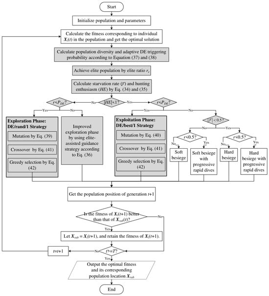
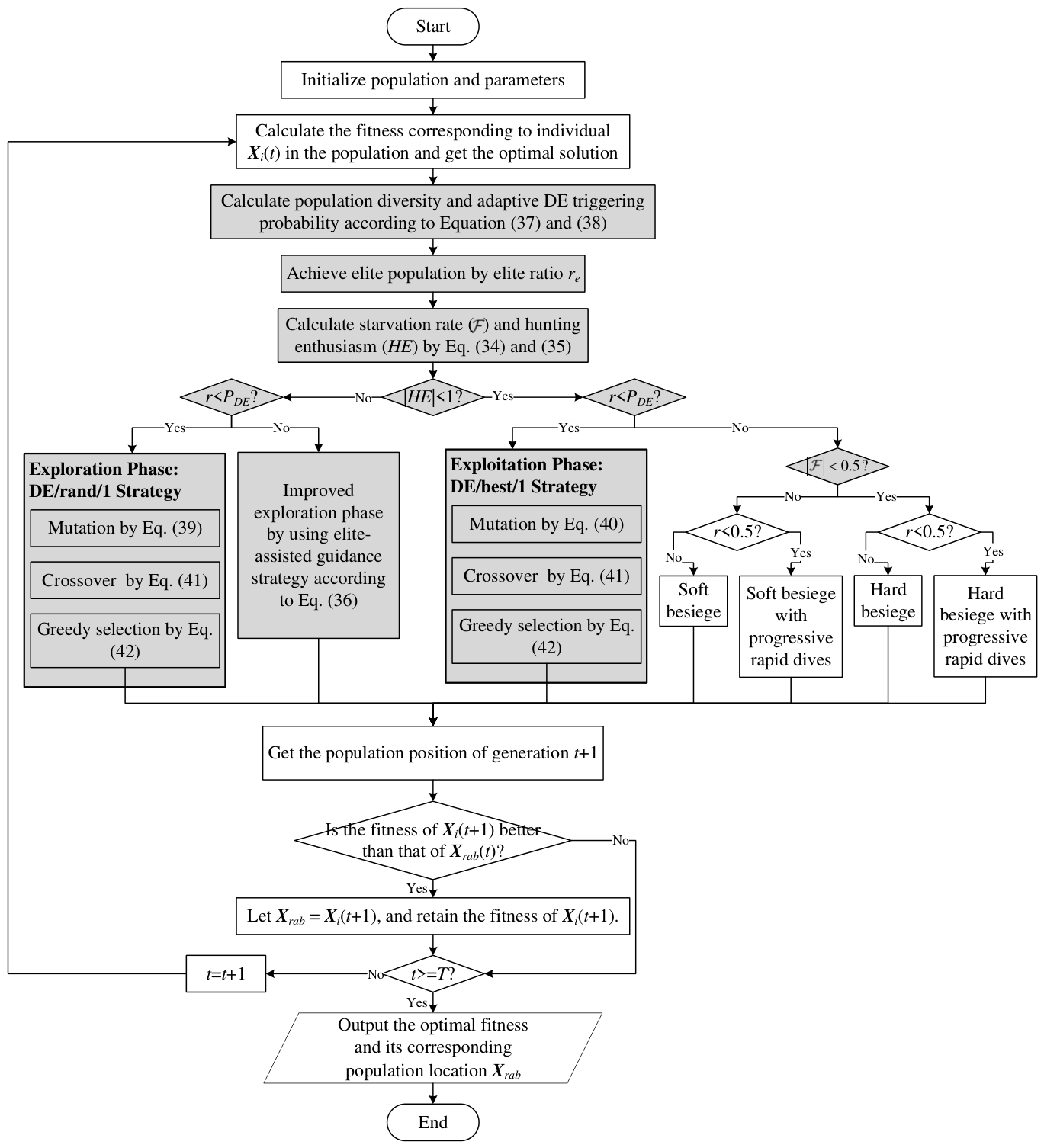
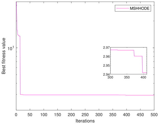
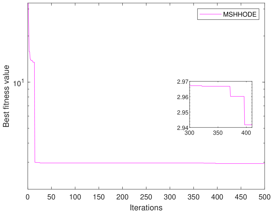
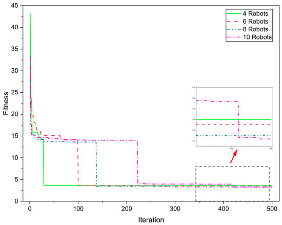
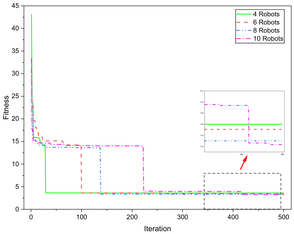
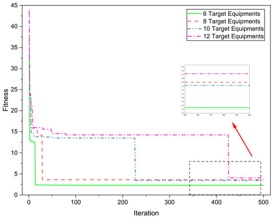
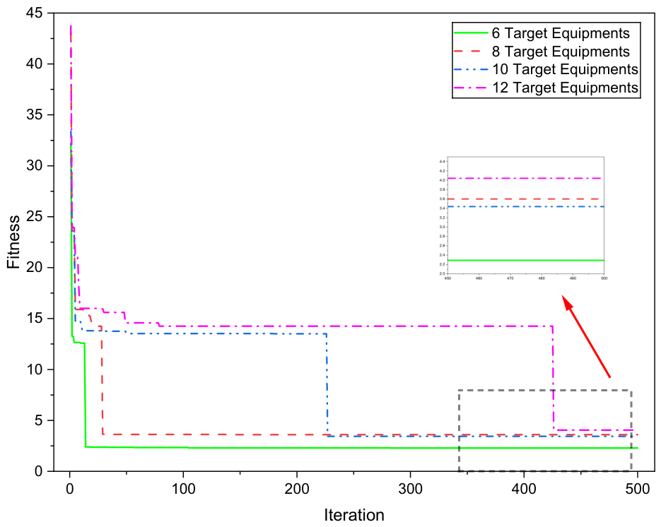
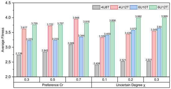
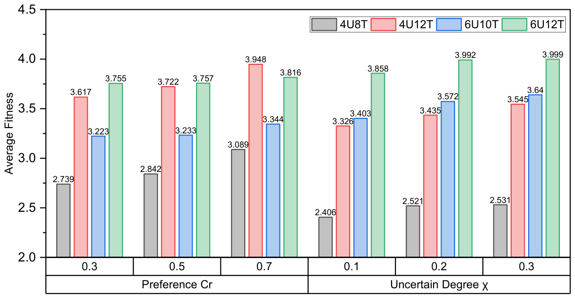
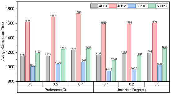
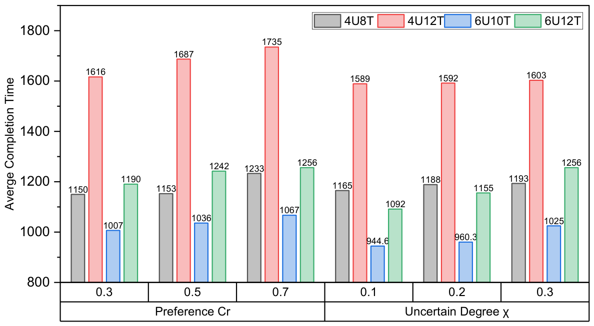
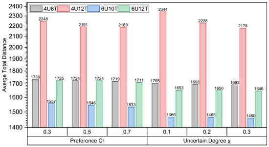
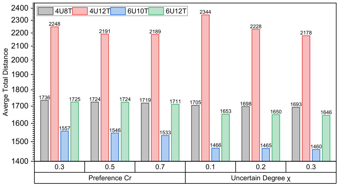
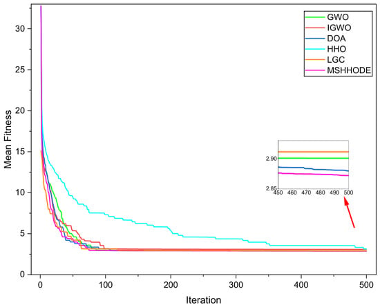
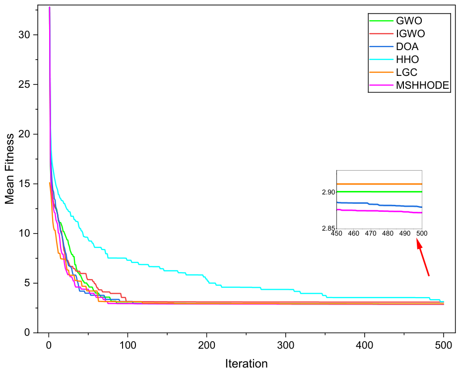
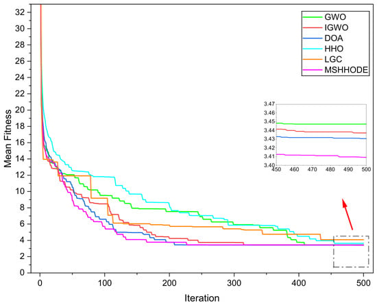
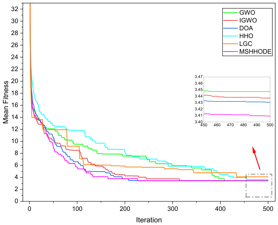
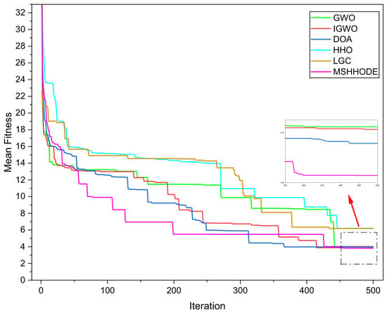
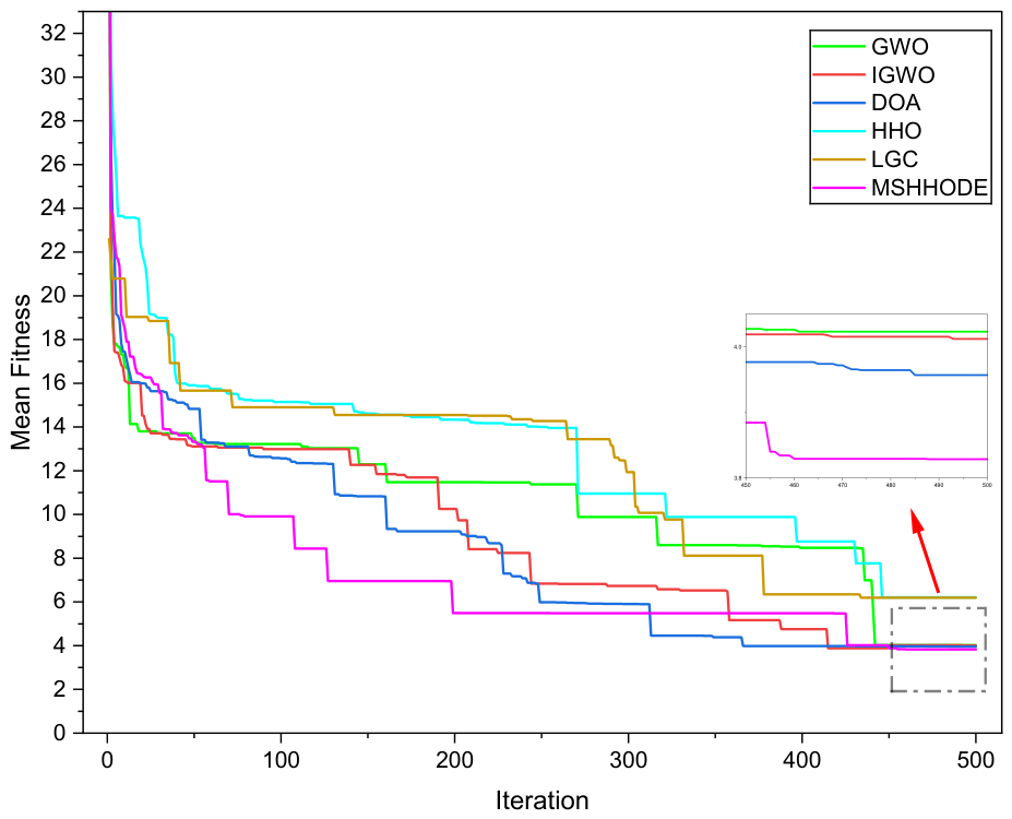
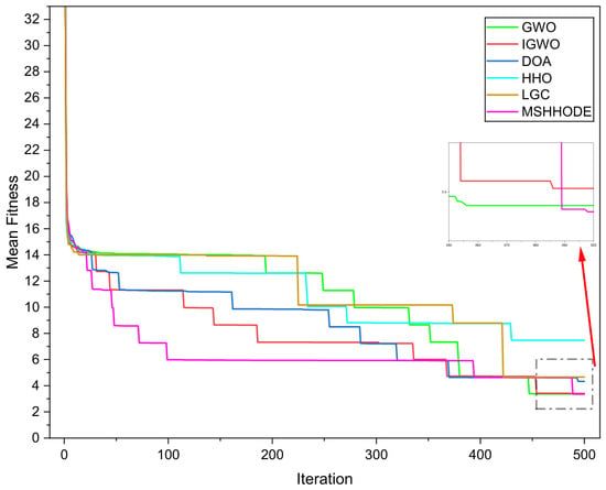
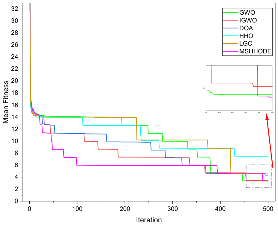
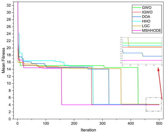
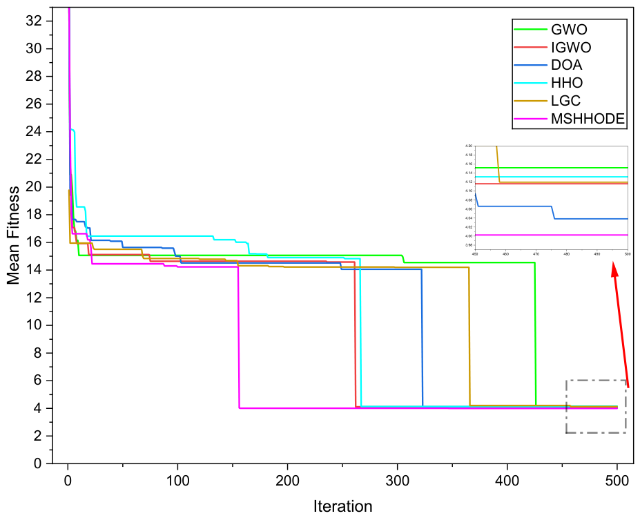

Disclaimer/Publisher’s Note: The statements, opinions and data contained in all publications are solely those of the individual author(s) and contributor(s) and not of MDPI and/or the editor(s). MDPI and/or the editor(s) disclaim responsibility for any injury to people or property resulting from any ideas, methods, instructions or products referred to in the content. |
© 2026 by the authors. Licensee MDPI, Basel, Switzerland. This article is an open access article distributed under the terms and conditions of the Creative Commons Attribution (CC BY) license.