


Abstract
Water-intensive industries in the Mediterranean face supply stress and decarbonisation pressure simultaneously. We develop an operations-research decision-support framework that treats the firm as one node of a small industrial resource cluster and prices the cost and carbon-equivalent emissions of five alternative supply trains—municipal water, river water, groundwater, rainwater harvesting and brewery wastewater reuse—within a multi-objective Linear Program. Each train carries engineering-grounded expenditures, energy intensities and grid emissions, and a weighted-sum scalarisation is solved daily for 365 days under three managerial scenarios. On a Cretan microbrewery whose 2022 demand of 5250 m3 is met from the municipal network, the balanced and cost-focused scenarios coincide on a single optimum that cuts the Levelised Cost of Water by 25.3% and emissions by 40.7%, while the eco-friendly scenario yields a 19.3% cost and 51.7% emissions reduction. LP duality, shadow prices and an extended sensitivity programme (diversification, capacity, grid factor, discount rate, RO recovery and demand profile) turn the optimisation into a decision-support package: optimal daily allocations, shadow-price signals on capacity and demand, and robustness diagnostics for capital planning, dispatch and risk management. Results are site-specific, but the framework and its diagnostics transfer in structure to clusters sharing the same convex-polytope source geometry; transposition to energy cooperatives is future work.
1. Introduction
Industrial water supply has moved from the periphery to the centre of operational decision-making in water-intensive sectors. Climate-driven scarcity is reshaping the cost and reliability of conventional municipal supply, and the parallel imperative to decarbonise process operations is pricing the energy intensity of every cubic metre that crosses a plant boundary [1,2]. Diversification across multiple supply trains has therefore migrated from procurement to a multi-objective allocation problem within a small industrial resource cluster: a firm that buys five different waters at the gate must also operate five different treatment trains, each with its own techno-economic, energy and emissions signature, and trade those signatures off at daily resolution. Cast that way, the problem belongs to operations research and decision support: the formal kernel is multi-objective optimisation under capacity, demand and policy constraints, and the deliverable is an auditable allocation rule for managers, regulators and external stakeholders.
The Mediterranean Basin is the geographic context in which the problem is sharpest. The region warms roughly 20% faster than the global mean, displays one of the strongest precipitation declines in the CMIP5 and CMIP6 ensembles, and hosts aquifers in retreat across Greece, Spain and the Maghreb [3,4,5]. Groundwater extraction in the region has reached a regulatory inflexion point: a recent geophysical reconstruction attributes 6.24 mm of global sea-level rise between 1993 and 2010 to net groundwater abstraction [6], and southern European aquifers display chronic seawater intrusion [7,8]. Within this picture, the food-and-beverage industry is among the most water-intensive economic sectors; global brewing alone draws 5–10 L of water per litre of finished product, with the European industry mean reported at 4.6 L L−1 [9], and a textbook setting for the water–energy–food nexus framing that process systems engineering has developed over the past decade [10]. Global beer production exceeded 1.86 billion hectolitres in 2021 [11,12]. Even microbreweries place a non-trivial load on a stressed local water budget, particularly when supply is concentrated in months when surface water and aquifers are at their seasonal minima [9,13,14].
Integrated water resource management combines demand-side and supply-side measures, with supply diversification at industrial-site scale increasingly prominent in both [2,15]. The same logic of diversification, multi-actor coordination and shared infrastructure that animates the energy-cooperative and industrial-cluster literatures, from renewable-energy cooperatives and agri-energy collectives [16] to maritime and industrial-symbiosis clusters, is increasingly imported into industrial resource management, where the firm becomes one node in a small cluster of supply trains that must be jointly planned, dispatched and audited. The operational translation of that principle at the level of an individual industrial site, however, remains underdeveloped. Two largely disconnected bodies of work coexist. The first profiles the techno-economic and environmental performance of individual alternative sources, treatment train by treatment train: brackish-groundwater reverse osmosis [17,18], rainwater harvesting and treatment to potable standards [19,20,21,22], one-step reverse osmosis from riverbank-filtered surface water [23,24], and multi-stage membrane reuse trains for brewery effluent [25,26,27,28,29]. The second optimises the inter-sectoral allocation of an aggregate water budget at basin or municipal scale, predominantly with population-based metaheuristics that produce Pareto-frontier solutions for public planners [30,31,32,33,34]. Embedding several treatment-train alternatives within a single firm-level operations-research decision tool, at daily resolution, with explicit emissions accounting and governance-relevant duals, has not, to the authors’ knowledge, been addressed.
The present paper develops such a tool. The LP kernel itself is a well-established operations-research instrument [35,36]; the contribution lies in coupling it to a treatment-train-grounded cost-and-emissions matrix and embedding it within an industrial-cluster decision frame. Concretely, a linear-programming kernel allocates daily water intake across five alternative sources subject to capacity, demand and pre-screening constraints, scalarising cost and carbon-equivalent emissions through a weighted sum. The framework is parameterised against a real Cretan microbrewery and solved on a 365-day capacity profile under three plausible managerial weightings. Four design choices distinguish the contribution from prior work and align it with the operations-research and decision-support tradition.
First, every cost and emissions coefficient is traceable to a documented treatment-train design, membrane lifetime, equivalent annual cost, energy intensity and grid emission factor, so that the LP coefficients are engineering-grounded unit-process metrics rather than abstract supply prices. Second, the temporal resolution is daily, capturing seasonal river flow, dynamic rainwater-tank accumulation and the operational-day demand profile that determines reuse availability. Third, the framework treats the firm as a node within an industrial resource cluster whose five supply trains can be governed jointly, with linear-programming duality (shadow prices on capacity and demand) supplying the marginal-value signals that a coordinator of the cluster needs to evaluate diversification ceilings, capacity investments and operating policies. Fourth, the analysis layer documents two structural findings rarely surfaced in basin-scale work, such as a coincident optimum between the cost-focused and balanced scenarios under the local source matrix, and a band-shaped diversification penalty that supports a simple, transferable regulatory recommendation.
Linear programming is preferred over population-based metaheuristics because the daily allocation problem is linear and convex, so a deterministic LP returns a certifiable global optimum together with shadow-price duals at a fraction of the computational and reproducibility cost of NSGA-II, CSS, ARNSGA-III or hybrid Whale-Optimisation alternatives [30,31,32,33]; the full geometric and dual argument is set out in Section 3.6. The framework is therefore positioned as complementary to the metaheuristic basin-scale allocation literature, not competitive with it.
The rest of the paper is organised as follows. Section 2 reviews the alternative-source treatment literature, the multi-objective allocation literature and the adjacent operations-research and industrial-cluster scholarship that motivate the framing, and articulates the research gap. Section 3 develops the framework, the LP formulation, the LP-geometry and shadow-price diagnostics, and the sensitivity-analysis design. Section 4 presents the results, including the grid-factor parametric sweep that bounds the transferability of the headline numbers. Section 5 discusses the implications, places the LCOW values against published industrial benchmarks, locates the framework in the operations-research and industrial-cluster decision-support literatures, and draws governance and innovation-management implications for water-intensive industries and energy-resource cooperatives. Section 6 concludes.
2. Related Work and Research Gap
2.1. Alternative Water Sources and Treatment Trains for Industrial Users
Five alternative water sources dominate the industrial-scale literature: groundwater, rainwater harvesting, river water, water reuse and seawater desalination. Of these, the first four are directly applicable to inland small and medium industries; desalination, by contrast, requires coastal proximity and is excluded from the present analysis on grounds of facility location.
Groundwater. Groundwater remains the principal industrial alternative to municipal supply across southern Europe, but its exploitation has reached a regulatory inflexion point [7,8,37]. Treatment economics for industrial users are dominated by reverse osmosis when feed water is brackish, with capital and operational expenditure analyses available across a wide capacity range [17,18]. Lower-cost alternatives such as ion exchange, electrodialysis reversal and nanofiltration may be substituted for RO when contaminant profiles allow; Da’ana et al. [38] survey low-cost options for toxic-element and microbial removal. Industrial-demand modelling [39] confirms that price and quality jointly drive substitution between groundwater and publicly supplied water. The carbon footprint of pumping and treatment is increasingly quantified through life-cycle assessment, capturing both direct energy use and the carbon intensity of the local electricity mix [40,41].
Rainwater harvesting systems (RWHS). Rainwater harvesting is well established as a Mediterranean-appropriate climate-adaptation measure. Farreny et al. [19] demonstrated cost-efficient designs for dense Mediterranean neighbourhoods, and Kakoulas et al. [20] confirmed effectiveness in the Greek-island context with detailed component-level pricing. Quality concerns once concentrated on roof-borne contamination [42,43]; recent monitoring of Greek urban precipitation has detected measurable cytotoxicity even in airborne rainfall [44], reinforcing the need for treatment trains beyond simple chlorination when potable use is intended. Treatment options now converge on multistage designs combining sand or carbon filtration, ultrafiltration and ultraviolet disinfection [21,45,46,47]; LCAs of decentralised potable systems report energy intensities in the range of 4–6 kWh m−3 [22]. Climate-projection studies indicate that RWHS reliability remains adequate at the household scale, although industrial-scale applications are capacity-constrained by storage volume and roof catchment area [48].
River water. River water occupies an ambivalent position. It is one of the cheapest treated alternatives where flow is reliable, but in the Mediterranean, seasonality and abstraction limits make it a partial source rather than a primary one [49,50]. Riverbank filtration is well validated as an in-situ pre-treatment that exploits natural soil filtration to reduce turbidity, organics and pathogens [23]. The recent One-Step Reverse Osmosis concept couples riverbank (or artificial bank) filtration with a single RO stage and reports particle, pathogen and organic micropollutant rejection above 99.9% at lower capital cost than conventional sequential trains [24]. Quartz-sand biofiltration provides a still cheaper treatment for non-potable uses [51]. Cretan rivers have been characterised at basin scale through the Soil and Water Assessment Tool and its karst-flow extension, producing the per-second flow data that any local industrial application must inherit [52,53].
Water reuse. Water reuse has progressed from a niche option to a mainstream industrial decarbonisation lever, particularly for the brewing industry where effluent volumes are substantial, and quality is heavily organic-loaded [54,55,56,57,58]. Process options now centre on multi-stage membrane trains. Holloway et al. [25] compared microfiltration/RO/ultraviolet advanced oxidation against hybrid osmotic-membrane bioreactor configurations under a life-cycle lens. Tay et al. [26] demonstrated nanofiltration-MBR + RO at 90% recovery, outperforming the equivalent ultrafiltration-MBR + RO at 75%. Within brewing specifically, Werkneh et al. [27] reviewed bioreactor-based brewery wastewater treatment with energy recovery, while Toran et al. [28] assessed UF-RO and ozonation–coagulation–MF–RO trains under realistic membrane-fouling regimes. Verhuelsdonk et al. [29] performed a Monte-Carlo cost evaluation of a full-scale flotation–MBR–UF–RO scheme, reporting economic viability in 77.2% of simulated cases at a treated-water cost of 1.80 EUR m−3.
2.2. Multi-Objective Allocation Algorithms and the Operations-Research Lineage
Multi-objective water-resource allocation has been an active operations-research subfield for two decades; representative recent works are summarised in Table 1. Asadieh and Afshar [30] introduced an Enhanced Charged System Search algorithm for hydropower-and-supply reservoir operation in Iran. Zhang et al. [31] coupled a hybrid Whale Optimisation Algorithm with a non-cooperative game to reconcile administrative-level interests in Handan, China. Tang et al. [32] balanced fairness and shortage risk through the ARNSGA-III algorithm in Wusu City. Zhang et al. [33] applied NSGA-II to intergenerational equity in the Huaihe River Basin, and Li et al. [34] used connection entropy to evaluate groundwater-exploitation modes in the southern Beijing plain. These works demonstrate the maturity of metaheuristic optimisation for inter-sectoral, basin-scale, multi-stakeholder problems, but they all adopt a public-planner perspective, abstract treatment-train economics into aggregate supply prices, and price emissions only indirectly through proxy environmental indices. They sit in a parallel methodological lineage to the linear- and mixed-integer-programming kernels used at firm scale in the operations-research literature on industrial energy and resource clusters [59,60,61,62], where deterministic optimisation, weighted-sum scalarisation and shadow-price duals provide the auditable backbone that decision-support practice requires. Table 1 presents Representative recent contributions on multi-objective water-resource allocation, contrasted with the present work. The two right-hand columns expose the contribution gap addressed here.
Table 1.
Comparison of this study to past research works.
2.3. Research Gap and Contribution
The literature reviewed in Section 2.1 and Section 2.2 establishes two well-developed but largely disconnected bodies of knowledge. The first profiles the techno-economic and environmental performance of individual alternative sources, typically through stand-alone treatment-train case studies. The second optimises the inter-sectoral allocation of an aggregate water budget at basin or city scale. Bridging the two at the level of the industrial firm that must commit to a specific blend of treatment trains, with capital expenditures locked in at design time and operational expenditures running daily, has received limited attention; equally absent from the brewery-sustainability literature is a decision-support tool that frames the firm’s multi-source supply problem as a small industrial resource cluster and exposes the LP duals that managers and regulators of such a cluster need. Existing diversification studies for urban water systems [15] confirm the directional benefits of multi-origin supply but stop short of a tractable, auditable optimisation tool that an industrial cluster manager could deploy.
The contribution of this paper is, accordingly, primarily a positioning contribution rather than an algorithmic one. The linear-programming kernel itself is well-established; what is novel is its coupling to a treatment-train-grounded cost-and-emissions matrix, its embedding within an industrial-cluster decision frame, and its application to a firm-level decision boundary. Within that frame, the paper makes five specific advances: In plain terms, the novelty is not a new optimisation algorithm but a firm-level application: engineering-grounded per-source cost-and-emissions coefficients, daily LP allocation across five real treatment trains, and a decision-support reading of both the primal allocations and the dual signals.
- Every LP coefficient is traceable to a documented treatment-train design and a Mediterranean-island grid emission factor, so the optimisation operates on engineering-grounded unit-process metrics rather than on abstract supply prices;
- The temporal resolution is daily across a full operating year, capturing seasonality, dynamic rainwater-tank accumulation and operational-day demand;
- Under the local source matrix, the cost-focused and balanced optima are shown to coincide—a structural finding that motivates a generalisable diagnostic for industrial-cluster managers: the explicit pre-check of cost-and-emissions vector alignment before reporting a trade-off as inherent;
- The framework outputs are read both as primal allocations and as dual signals (shadow prices on capacity and demand) that translate the LP solution into governance- and investment-relevant quantities for the cluster coordinator; and
- A four-axis sensitivity analysis stresses the optimum against per-source diversification bounds, drought-induced groundwater and river capacity shocks, and parametric variation of the grid emission factor, so the transferability of the headline numbers is bounded rather than asserted.
To make the methodological positioning concrete, the same daily allocation problem could in principle be solved by NSGA-II or another population-based metaheuristic [30,31,32,33]. For the present matrix this would deliver, at best, the same vertex optimum as the LP, because the feasible set is a convex polytope and the objective is linear, at the cost of (a) stochastic run-to-run variability that requires Monte-Carlo replication, (b) typical wall-times of minutes per scenario rather than milliseconds, and (c) absent dual variables, depriving the decision-maker of the shadow-price signal that the LP supplies for free. Where the present analysis runs all 365 daily LPs, plus the 19-variant four-axis sensitivity sweep (5 β-bounds + 5 γ-shocks + 5 ρ-shocks + 4 grid-factor recomputations) and the 41-step continuous weight sweep, in well under a minute on a single CPU core—each daily LP solving in roughly 1.6 ms and a full 365-day scenario in about 0.5 s (Section 4.8.6)—an equivalent NSGA-II implementation would consume orders of magnitude more time without improving solution quality. The framework therefore substitutes deterministic LP for metaheuristic search at the firm scale, while reserving metaheuristics for the basin-scale, non-convex multi-stakeholder problems for which they were designed.
3. Materials and Methods
For convenience to the reader, the indices, decision variables and parameters used throughout this section are summarised in Table 2; acronyms are expanded at first use and reproduced in the abbreviations list at the end of the manuscript.
Table 2.
Nomenclature for the multi-objective LP formulation.
3.1. Case Study: A Brewery as a Node Within a Small Industrial Resource Cluster
The framework is applied to a Cretan microbrewery in the western part of Crete, Greece. The plant produces unfiltered, unpasteurised draught craft beers and reported a 2022 water consumption of 5250 m3, corresponding to a water-to-product ratio of approximately 5:1, a value consistent with the European brewing-industry mean reported in recent water-footprint surveys [9]. Its current water supply is sourced exclusively from the local water utility (DEIAVA), and a reverse-osmosis polishing unit installed by the company guarantees the conductivity range required for brewing. The brewery is treated, in this paper, not as a stand-alone procurement boundary but as the single demand node of a small industrial resource cluster whose other members are the supply trains drawing from the municipal network, the Derianos river, the on-site well, the rainwater catchment and the brewery’s own effluent. Three of the five trains (utility, river, well) involve external regulators or operators, and only two (rainwater, reuse) are firm-internal, so the multi-actor character applies to the inter-train coordination problem rather than to every train individually; the framework’s role is to support that joint allocation decision across the cluster.
Three features of the site make it informative as a test bed for diversification analysis. First, the surrounding Tavronitis basin is hydrologically heterogeneous: it hosts 16 boreholes, 38 wells and a documented spring in addition to the river system itself [63], yet groundwater overexploitation is a documented concern [64]. Second, the brewery already owns an underused well within its property with a proposed groundwater extraction rate of 2.25 m3 h−1. Third, the wider Cretan agro-industrial landscape contains analogous small clusters (irrigation cooperatives, food-and-beverage SMEs, port operators) that face the same multi-source allocation problem, so the case-study design is chosen to be transposable rather than idiosyncratic. Together, these features supply a realistic laboratory for the deliberate diversification problem analysed below.
For modelling purposes, the daily water demand is assumed uniform across operational days. From the 365 calendar days of 2022, 62 are excluded (Sundays and public holidays), leaving 304 operational days; the resulting daily demand of 17.27 m3 d−1 supplies the LP demand vector . The uniformity assumption is an analytical simplification that trades realism in intra-week and seasonal production curves for transparency in the optimisation. Its directional effect is not intrinsically conservative: a summer-peaked brewery profile would stress the system more strongly during low-flow months, whereas a winter-peaked profile would make river substitution easier. Section 5.5 returns to this limitation.
3.2. Methodological Assumptions
Three simplifying assumptions support the formulation; each is justified below in terms of how it bounds the result.
Static capital expenditure. Capital expenditure (CapEx) is held constant during optimisation. This assumption is standard in techno-economic analyses of water-treatment systems because CapEx is intrinsically lump-sum and only loosely coupled to small variations in throughput. Treating CapEx as static yields a deterministic levelised-cost denominator and avoids the circularity of adjusting plant size to a yet-unknown optimal flow. The implication, per-cubic-metre CapEx that scales inversely with realised utilisation, is examined in Section 5.5 and motivates the nested-formulation extension proposed in Section 6. To be explicit, each treatment train is sized once at design capacity and assumed fully installed regardless of the realised daily throughput, so its lump-sum CapEx is recovered over the asset lifetime irrespective of utilisation; the consequences of varying the fixed discount rate are quantified in Section 4.8.1.
Reverse-osmosis recovery rate. RO stages are modelled with a 100% recovery rate. This abstraction omits brine handling and recovery-rate optimisation; in real installations, the recovery rate of brackish-water RO ranges between 60% and 90% [17,65]. A finite recovery rate would raise the effective LCOW for the river OSRO, groundwater and reuse pathways by approximately 10–40%, depending on the source-specific recovery and concentrate-management assumptions. The unit-cost values reported in Section 3.3 should therefore be read as lower-bound estimates when the framework is transposed to a plant operating at a finite recovery rate, and an explicit first-order recovery-rate sweep that quantifies these effects on both the per-source unit costs and the optimised solution is reported in Section 4.8.2.
Currency and discount rate. All monetary values are expressed in 2022 euros. United States dollars and euros are taken at parity (1 USD = 1 EUR), reflecting an average exchange rate of approximately 1.05 USD/EUR over the 2022–2023 data-collection window. Other currencies (Vietnamese dong, Australian dollars, British pounds) are converted at the spot rate at the source-publication date. Capital expenditures are amortised through the Equivalent Annual Cost formulation [65]:
where is the initial capital cost (EUR), the discount rate, and the asset lifetime (yr). The discount rate is fixed at = 0.10 across all components, consistent with techno-economic studies of Mediterranean-island infrastructure where the higher cost of capital relative to mainland Europe is well documented [59].
3.3. Source-Specific Treatment Design and Unit Costs
Five candidate sources are characterised in turn. The treatment train, capacity, EAC inputs, electricity intensity, and resulting unit cost (EUR m−3) and unit emissions (kg CO2eq m−3) for each source are summarised in Table 3 and Table 4.
Table 3.
Treatment train, lifetime and EAC inputs for the five candidate sources.
Table 4.
Aggregate unit cost and unit emissions used as LP coefficients.
3.3.1. Municipal Network Water
The municipal supply is polished through a single-pass RO system to remove residual minerals and ions. A KYRO-1000 reverse-osmosis plant (1000 L h−1 nominal capacity, 2.25 kW, 2500 USD purchase, = 10 yr) is sized to absorb the brewery’s annual demand at an 18-h effective workday. Maintenance is dominated by membrane replacement; conservatively, a 1000 EUR membrane stack is assumed to be replaced every 5 yr, consistent with the lifetime adopted by Jamil et al. [65] for desalination service. Municipal water is purchased at the tariff structure published by the neighbouring Chania utility (DEIACH), used as a proxy for the unpublished DEIAVA tariff; quarterly invoicing of a uniformly distributed annual consumption yields a blended purchase cost of 1.09 EUR m−3.
The energy footprint of the municipal supply chain is taken from the Mediterranean-conditions LCA of Amores et al. [66]. The five-stage chain (water abstraction 0.294, potable-water-treatment plant 0.071, intermediate pumping 0.154, distribution 0.304 and wastewater-treatment plant 1.090 kWh m−3) sums to 1.913 kWh m−3 on the supply side. The on-site RO polishing unit adds a further 0.225 kWh m−3. Following [66], the bidirectional nature of the urban water cycle is accounted for by recognising that the brewery’s effluent re-enters the network and re-traverses the wastewater-treatment and distribution stages; the bidirectional accounting raises the effective intensity to approximately 4.281 kWh m−3, the value used as the LP coefficient. This bidirectional accounting is conservative: a one-directional treatment that excludes effluent return would yield a lower intensity (≈2.14 kWh m−3), which would shrink the headline emissions reduction by approximately one-third without changing the qualitative findings.
The conversion to carbon-equivalent emissions follows the Cretan electricity-grid emission factor of 0.989 kg CO2eq kWh−1 [59] and a primary-energy factor of 2.9, yielding a unit-emissions value of 12.279 kg CO2eq m−3, the highest among the five candidate sources. The Cretan-island grid is unusually carbon-intensive because the island still derives most of its electricity from heavy-fuel-oil generation; on a less carbon-intensive grid, the absolute gap between municipal water and the alternatives shrinks proportionally. This dependency is explored quantitatively in Section 4.6. The volumetric capacity of the municipal source is set to 100 m3 d−1, a value large enough to act as a soft “infinite” supply within the LP solver while keeping the bounds finite.
3.3.2. River Water
The Tavronitis tributary, the Derianos River, runs adjacent to the brewery facility but exhibits strongly seasonal flow, with multiple summer days at zero discharge. Daily flow data for 2020 simulated by the SWAT/KSWAT karst-hydrology models of Malagò et al. [52] and Nerantzaki et al. [53] are inherited as a proxy for the 2022 hydrological year; comparisons with regional precipitation indices indicate that 2020 and 2022 were similarly dry years, so the proxy is conservative. To respect documented stress on Greek river basins [49], only a 10−4 fraction of the simulated daily flow is treated as exploitable; the resulting capacity vector feeds the LP as U2(t). A sensitivity row in Section 4.5 stresses this assumption.
The treatment train follows the One-Step RO concept of Zhai et al. [24], coupling artificial bank filtration (used in place of riverbank filtration because Derianos is non-perennial) with a single RO polishing stage. CapEx is scaled from a reference plant cost of 14 M EUR at 28,400 m3 d−1 daily capacity [67] using the standard power-law cost-scaling relationship,
with C1 = 14,000,000 EUR, Q1 = 28,400 m3 d−1, Q2 ≈ 14 m3 d−1 (matching the local annual-sum capacity of 5096 m3) and = 0.75. The choice = 0.75 lies inside the empirical range reported by Tribe and Alpine [68] and is used as a central estimate for a modular small-scale OSRO skid; as discussed in Section 3.6.2, a classical 0.6-rule exponent would predict a substantially higher scaled CapEx for this severe downscaling case. The scaled plant CapEx evaluates to 46,300 EUR; an assumed 25-year lifetime and = 0.10 give an EAC of 5099 EUR yr−1 and a per-cubic-metre CapEx of 1.001 EUR m−3. Operating expenditure is partitioned into electricity and membrane maintenance following the breakdown reported by Zhai et al. [24]; the median electricity intensity of 0.615 kWh m−3 is repriced at the Greek tariff of 0.22 EUR kWh−1, yielding an LCOW of 1.522 EUR m−3.
3.3.3. Groundwater
The on-site well is modelled as a 60–70 m deep aquifer abstraction point. A submersible pump is sized for a flow of 2.25 m3 h−1 against a total dynamic head of 84.5 m (static head plus a 30% friction allowance, an industry-standard margin for vertical pipe runs of this length). The Ebara OYM 4N2-20/1.1 (1.1 kW, 1038 EUR purchase, = 10 yr) was selected after a manufacturer-side selection tool comparison among the Ebara, Grundfos, and Franklin lines using the published H–Q efficiency curves; the chosen pump operates within its best-efficiency range at the design point, minimising lifetime energy consumption. Operational hours are bounded at 5 h d−1 for 304 d yr−1, a conservative regime designed to avoid contributing to the documented over-extraction of the Tavronitis aquifers [64]. The post-extraction treatment combines two RO units in tandem (KYRO-2000 + KYRO-500, 2.5 m3 h−1 aggregate, 5 kW total, 6950 EUR total purchase), driven by the higher likelihood of salinity in groundwater than in the polished municipal feed [18]. The membrane stack is replaced every 5 yr at a 2000 EUR cost.
The pump and tandem-RO combination consumes 1520 h yr−1 × 1.1 kW = 1672 kWh yr−1 at the pump and 1520 h yr−1 × 5 kW = 7600 kWh yr−1 at the RO stage, for a combined 9272 kWh yr−1. Distributed over the 3420 m3 yr−1 that this regime delivers, the energy intensity is 2.711 kWh m−3. The aggregate LCOW of 1.131 EUR m−3 makes groundwater the cheapest source in the matrix; its emissions translate, through the same grid-factor and primary-energy-factor chain as the municipal source, to 7.775 kg CO2eq m−3, lower than the municipal pathway but higher than river OSRO. The combination of the lowest cost and the second-lowest emissions accounts for groundwater’s dominance in every solved scenario.
3.3.4. Rainwater Harvesting
The harvest potential is calculated from the standard rational equation,
where (m3) is the daily harvested volume, the catchment area (m2), the dimensionless runoff coefficient, and daily precipitation (m). Daily precipitation for the 2022 hydrological year was retrieved from NASA’s POWER Data Access Viewer [69] for the brewery coordinates. A roof catchment area of 580 m2 is measured from satellite imagery, and is fixed at 0.9, a typical and conservative value for industrial rooftops [70]. Annual precipitation totalled 452 mm in 2022, lower than the 1958–2010 long-term mean (615 mm) recorded at the nearby Souda meteorological station; the annual harvest is 238.4 m3.
The treatment train follows Tran et al. [21] and is corroborated by Yan et al. [22]: a 16 m3 polyethene storage tank, a pre-filtration rainwater filter, a complex multi-stage filtration unit (fibre + carbon + ultrafiltration) and a 12 W ultraviolet disinfection lamp. CapEx is benchmarked against the Greek island prices reported by Kakoulas et al. [20] for tank, pump, and ancillary equipment; the unit-process cost references in [21] are inflated by a 1.5 multiplier to bridge the price gap between the Vietnamese reference market and the Greek market. The reference design specifies two pumps and two UV bulbs; the present implementation uses one of each, so the energy budget is reduced from the published value, but only by 35% rather than the naïve 50%, to avoid underestimating ancillary balance-of-plant consumption. The aggregate LCOW of 5.382 EUR m−3 is the highest in the matrix and is dominated by the small annual harvest volume across which the EAC is amortised; the energy intensity of 3.487 kWh m−3 translates to 10.001 kg CO2eq m−3.
The rainwater capacity profile differs structurally from that of the other sources. The storage tank acts as a buffer with a hard upper-volume cap of 16 m3, and the daily exploitable volume on day depends on the previous day’s residual. This dynamic accumulation rule is implemented as a state update on the U4(t) vector after each daily solution (Section 3.7).
3.3.5. Brewery Effluent Reuse
A flotation–MBR–UF–RO scheme adapted from Verhuelsdonk et al. [29] is used for the reuse pathway; its component-level CapEx and OpEx breakdowns are inherited at face value, given the relative proximity in time (paper received 2020) and in industrial type (German full-scale brewery) to the present case study. Aggregate CapEx of 137,475 EUR (flotation + buffer tank + MBR + UF + RO) yields an EAC per cubic metre of 0.32 EUR m−3 at = 15 yr and = 0.10. Operating cost is partitioned between electricity (the explicit MBR consumption is reported by Verhuelsdonk et al.; UF and RO are scaled by the published O&M-to-electricity ratio) and membrane maintenance; repriced at the Greek tariff of 0.22 EUR kWh−1, the LCOW reaches 2.05 EUR m−3. A 10% credit is applied to the energy footprint of reuse to capture, conservatively, the avoided environmental burden of effluent discharged to the municipal sewer [66]. A first-principles upper bound on this credit can be estimated as the avoided wastewater-treatment-plant energy share within the municipal pathway, (1.090/4.281) × 12.279 ≈ 3.13 kg CO2eq m−3; the chosen 10% credit (1.066 kg CO2eq m−3) is therefore deliberately conservative, sitting at roughly one-third of that upper bound and avoiding double-counting with the LCA scope already embedded in the municipal coefficient. The resulting unit emissions equal 9.594 kg CO2eq m−3.
The volumetric capacity of the reuse stream is set to the residual after subtracting the 2022 finished-product volume (889.82 m3) from the annual water consumption (5250 m3), yielding 4360 m3 yr−1 uniformly distributed across operational days, i.e., 14.34 m3 d−1. This is an upper-bound estimate; under genuine industrial practice, the daily reuse availability would be a function of the prior day’s actual consumption and effluent fraction, a refinement discussed in Section 5.5.
3.4. Aggregated Cost and Emissions Matrix
Table 3 and Table 4 consolidate the unit-process design, EAC inputs and per-cubic-metre cost and emissions used as the LP coefficients. The matrix encodes the two facts that drive much of the optimisation behaviour reported in Section 4. Groundwater is simultaneously the cheapest source in EUR m−3 and the second-cleanest in kg CO2eq m−3. River water is the cleanest source by a wide margin (1.764 kg CO2eq m−3, against 7–12 for the others) but only the second-cheapest, so its preference depends sharply on the relative weighting of cost and emissions. The daily exploitable capacity profiles for all five sources, alongside the daily demand profile, are plotted in Figure 1. The visualisation is deliberately compositional: every source is represented both by a time-series view (with a 30-day rolling mean to surface seasonal structure) and a monthly box-plot panel that shows within-month dispersion, with coefficient-of-variation annotations summarising the relative volatility of each series. The river Figure 1c shows the central hydrological constraint that drives the optimisation: river capacity is highly skewed, with most of the annual flow concentrated in the November–April window and multiple summer days at zero discharge, reflecting the Mediterranean karst-flow regime that the SWAT/KSWAT models reproduce [52]. The rainwater Figure 1e shows the residual after the dynamic tank-accumulation rule has been applied; the discrete spikes correspond to single rain events that fill the buffer to the 16 m3 ceiling. By contrast, the deterministic Figure 1b,d,f act as visual control, showing that municipal, groundwater and reuse availability provide the steady backbone over which the volatile river and rainwater sources fluctuate.
Figure 1.
Daily water demand of the Charma microbrewery and the exploitable capacity profile of each of the five candidate sources across the 2022 hydrological year.
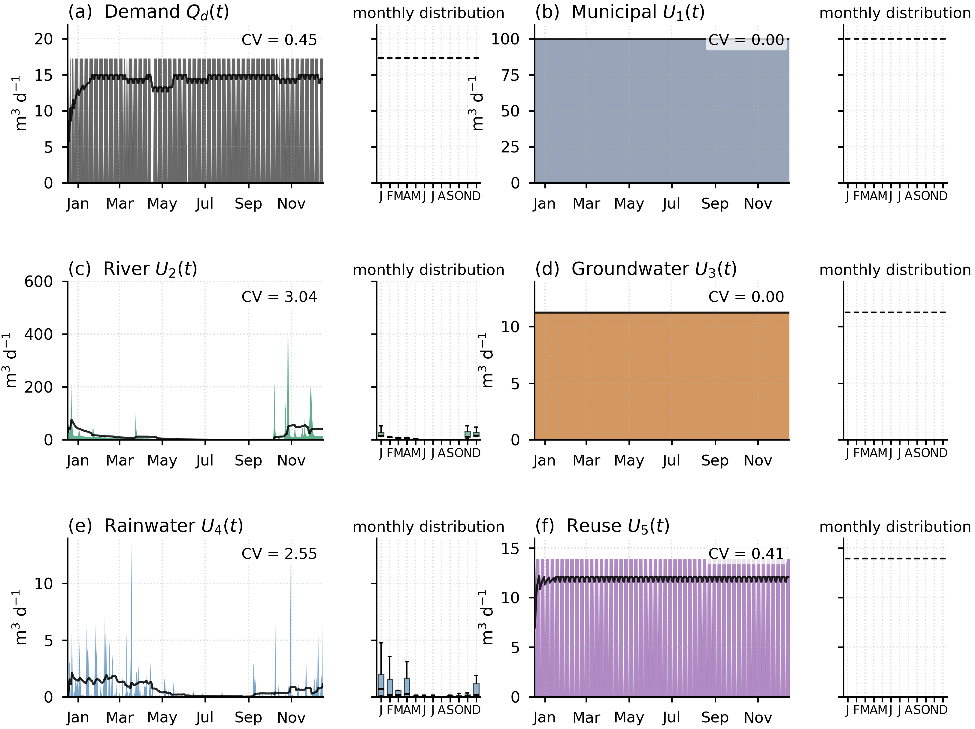
The composite is structured to show three orthogonal aspects of each input series simultaneously. The main time-series sub-panels (Figure 1a–f, left of each pair) plot the raw daily values together with a 30-day rolling-mean black trace that suppresses high-frequency noise and emphasises seasonal structure. The right-hand box-plot sub-panels show the same series aggregated into twelve monthly distributions, summarising within-month variability that the time-series view conceals. The annotated coefficient of variation (CV = σ/μ) provides a single scalar summary of each series’ relative dispersion. CV is essentially zero for the deterministic municipal, groundwater and reuse capacities; 0.45 for demand (driven by the operational/non-operational day pattern); 2.55 for rainwater (the discrete dry-day-versus-rain-day pattern); and 3.04 for the river, the largest of the matrix and the principal driver of the seasonal allocation behaviour reported in Section 4. Figure 1a plots the daily water demand; Figure 1b–f plot (Municipal), (River), (Groundwater), (Rainwater) and (Reuse) on a common time axis from 1 January to 31 December 2022.
3.5. Multi-Objective LP Formulation
For each operational day ( = 1, …, 365), let the decision variables be the daily volumes drawn from each eligible source, with ∈ , where ⊆ {1, …, 5} is the eligible-source subset defined below. The capacity envelope of source on day is , the daily demand is , and the unit cost and unit emissions are and (Table 4). Cost and emissions are each min–max-normalised across the source coefficients,
so that both terms enter the objective at unit scale before scalarisation; the normalisation is performed once before the daily loop. Min–max normalisation is preferred over z-score normalisation here because the source coefficients are bounded in physical units and have no underlying probability distribution to standardise against, and over no-normalisation because the raw kg CO2eq m−3 coefficients are roughly an order of magnitude larger than the EUR m−3 coefficients and would otherwise dominate the scalarised objective regardless of weight. Eligibility is determined by a pre-screening filter that admits source to only if its annual capacity reaches the minimum-share threshold,
with the share threshold set to = 0.10 by default. The threshold operationalises the engineering judgment that a source whose annual capacity falls below 10% of demand cannot, in principle, contribute meaningfully across the year, and amortising the source’s lump-sum CapEx over so small a denominator yields an unfavourable per-cubic-metre cost. The = 0.10 value is conservative relative to typical industrial diversification policies, which often exclude sources contributing less than 5% of demand; the implications of relaxing the filter to = 0.05 are discussed in Section 5.5.
For each day the solver minimises the scalarised weighted-sum objective,
subject to
where + = 1 (re-scaled from the percentage form (65, 35), (90, 10), (10, 90) used to label the scenarios), Equation (7) enforces daily demand satisfaction, and Equation (8) restricts each source to within its instantaneous capacity. The weighted-sum scalarisation is preferred over an -constraint or a goal-programming formulation because it preserves linearity (and therefore convexity), and because the three managerial scenarios already span the relevant region of the cost–emissions plane without requiring the full Pareto frontier to be enumerated. Three managerial scenarios are defined by the (, ) pair:
Balanced scenario: (, ) = (0.65, 0.35), the default risk-averse blend that mildly privileges cost while pricing emissions explicitly.
Cost-focused scenario: (, ) = (0.90, 0.10), a cost-minimising posture appropriate to budget-constrained periods.
Eco-friendly scenario: (, ) = (0.10, 0.90), an emissions-minimising posture appropriate to firms with explicit decarbonisation commitments.
The three weight pairs are chosen to span the practically relevant range: a balanced default with explicit emissions pricing, a cost-dominated extreme that sets emissions weight near zero, and an emissions-dominated extreme that almost reverses the priorities. Intermediate weights produce optima on the convex hull spanned by these three corner solutions.
3.6. Mathematical Structure and Techno-Economic Interpretation
Section 3.3, Section 3.4 and Section 3.5 expressed the framework as a sequence of unit costs, an aggregation table, and a Linear-Programming objective. The present sub-section develops the mathematical and techno-economic structure that those expressions inherit, with three aims: to justify the per-unit metric used in the objective (LCOW) within a standard discounted-cash-flow framework, to expose the geometric properties of the LP that make the headline results predictable, and to analytically derive the pivot weights that the empirical sweep of Section 4.7 reveals. The five sub-subsections that follow are not new additions to the formulation; they document the mathematical foundations on which Equations (1)–(8) already rest.
3.6.1. Levelised Cost of Water as the Per-Unit Techno-Economic Metric
The Levelised Cost of Water (LCOW) is the natural per-unit techno-economic metric for an industrial water-supply system, mirroring the role that the Levelised Cost of Energy (LCOE) plays in renewable-energy economics [59]. For an asset of lifetime , capital cost , annual operating cost OpEx, annual maintenance cost , and a constant discount rate , the Net Present Value of the asset’s lifetime cost stream is:
where the discount factor (1 + )−t captures the time value of money. The Equivalent Annual Cost (EAC) of the same asset is defined such that an annuity of EAC paid for years has the same present value as the cost stream:
When applied to a lump-sum capital expenditure with no recurring component, Equation (10) reduces to Equation (1). The LCOW per cubic metre is then the sum of the amortised capital, operating, and maintenance components divided by the annual treated volume Vannual:
The structure separates lump-sum capital expenditures—which would otherwise dominate per-cubic-metre costs at low utilisation—from operating expenses that scale with throughput. It is the LCOW that the LP minimises through the cost vector in Equation (6), with each computed via the EAC chain documented in Table 3 and Table 4. This separation also clarifies why a sensitivity sweep on the discount rate (Section 5.5, future-work item) would only affect the CapEx-amortised component of LCOW, not the OpEx component.
The discount rate = 0.10 was selected as a conservative central estimate consistent with techno-economic studies of Mediterranean-island infrastructure where the higher cost of capital relative to mainland Europe is documented [59]. A sensitivity analysis at ∈ [0.05, 0.15] would change the EAC of every CapEx-heavy source through the inverse-amortisation factor in Equation (1); evaluating that factor at the asset lifetimes of Table 3 yields swings of roughly +40% at = 0.15 and −36% at = 0.05 relative to the = 0.10 reference. Because OpEx-heavy sources and CapEx-heavy sources respond differently to , the exact ranking should be rechecked before transposition to another site; in the present matrix, however, the large gap between groundwater and the high-CapEx rainwater pathway makes the headline optimum unlikely to be overturned by discount-rate variation alone. When applied to a lump-sum CapEx with no recurring component, Equation (10) reduces directly to Equation (1) because the present-value term in the numerator collapses to and the denominator is the same annuity factor. This analytical estimate is now confirmed empirically (Section 4.8.1): re-solving the LP across r ∈ [0.05, 0.15] moves the optimised Balanced LCOW from 1.20 to 1.44 EUR m−3, and for r ≤ 0.08 the cheaper river-OSRO capital cost pulls the optimum across the first weight pivot into the river-leaning intermediate regime (unit emissions 6.27 instead of 7.28 kg CO2eq m−3), while the groundwater-led structure is preserved throughout.
3.6.2. Power-Law Cost Scaling and the Tribe-Alpine Exponent
Equation (2) applies a power-law scaling between a reference plant of known capital cost C1 and capacity Q1, and a target plant at capacity Q2. The scaling exponent captures the economy or diseconomy of scale: < 1 indicates economies of scale (a smaller plant costs proportionally more per unit capacity than the reference); = 1 indicates linear scaling; > 1 indicates diseconomies (rare in process industries). The functional form has a long history in chemical-process economics [71] and better reproduces a wide range of process-equipment cost data than alternative parametric forms, because the cost of small-scale unit processes contains a substantial fixed component (instrumentation, civil works, control systems) that pure volumetric scaling would not capture.
The choice = 0.75 lies inside the empirical range reported by Tribe and Alpine [68], who collected values between 0.6 and 0.95 across factory-equipment categories. The exponent governs how the predicted CapEx changes when the target capacity is much smaller than the reference plant: the smaller is, the steeper the economy of scale at the reference and, equivalently, the larger the predicted CapEx becomes when Q2 ≪ Q1. For the present downscaling from 28,400 m3 d−1 to ≈ 14 m3 d−1 (a factor of about 2000), the classical 0.6-rule prediction is 14,000,000 × (14/28,400)^0.6 ≈ 145,100 EUR—roughly 3.1 × the value obtained at = 0.75 (46,300 EUR). The choice = 0.75 is therefore the less conservative of the two; it produces a lower scaled CapEx and a lower river-water unit cost than the 0.6-rule would. Adopting = 0.75 is justified by the empirical evidence that the 0.6-rule can over-shoot for highly modular small-scale water-treatment skids relative to the chemical-process equipment that informed the original rule [71]. An sensitivity sweep across [0.6, 0.85] would shift the river-water LCOW materially and may change the river’s cost rank relative to reuse; the emissions-side role of river water would remain, but the cost-side contribution should be treated as conditional on the selected scaling exponent.
3.6.3. LP Geometry: Convexity, Vertex Enumeration, and the Pareto Frontier
The daily Linear Program of Equations (6)–(8) has a feasible set defined by linear equalities and inequalities, which is by construction a convex polytope ⊆ ℝ^|S| for each day . The objective function (Equation (6)) is linear, so by the Fundamental Theorem of Linear Programming, the optimum is attained at a vertex of , or along an edge in the degenerate case of multiple optima [35]. Vertices of correspond to basic feasible solutions in which exactly |S| − 1 of the constraints in (8) are active; at each vertex, at most one source operates strictly between zero and its capacity, while every other source either contributes nothing or saturates its daily cap.
Two consequences follow from this geometric fact and are central to interpreting the results of Section 4. First, the LP solver returns a certifiable global optimum for each daily problem, and a unique optimum unless multiple vertices share the same objective value. Interior-point LP algorithms provide polynomial-time guarantees; the HiGHS dual-simplex backend used here is selected for numerical reliability and resolves each daily problem in milliseconds on a single CPU core, so the 365 sequential daily solves complete in under one second of wall time. Second, as the weight pair (, ) varies continuously, the optimum jumps between vertices at a finite set of pivot weights: explicit values at which the linear objective becomes parallel to a face of . Between pivots, the optimum is constant in the source mix, which is the formal cause of the step-function structure that the continuous weight sweep of Section 4.7 traces out.
The Pareto front connecting the cost-optimal vertex (extreme cost-leaning weight) to the emissions-optimal vertex (extreme emissions-leaning weight) is therefore a piecewise-linear convex curve in (LCOW, EI) space. The frontier touches a finite set of vertices, three in the case study, as the cross-scenario tables of Section 4.4 will report, and the named scenarios in Table 5 and Table 6 represent samples of those vertices rather than continuous interpolations between them. The Pareto curve is convex because both objectives are minimisation targets and the feasible set is convex; under those conditions, the weighted-sum scalarisation of Equation (6) recovers the supported frontier as the weight pair varies over [0, 1]2 with + = 1 [36]. This is a sufficient theoretical justification for the parametric weight sweep of Section 4.7.
Table 5.
Annual contribution by source for each scenario (m3 yr−1), with capacity utilisation as a percentage of the calendar-year theoretical maximum.
Table 6.
Cross-scenario comparison of post-optimisation LCOW and unit emissions, with per cent change relative to the municipal-only baseline.
3.6.4. Analytical Derivation of the Weight Pivots
The two pivots reported by the empirical sweep of Section 4.7 are not artefacts of the numerical solver; they can be derived analytically from the per-source objective contributions. After min–max normalisation across the four eligible sources = {Mun, Riv, GW, Reuse} (rainwater is excluded by Equation (5); the analytical pivots derived below are accordingly conditional on this active source set, and a different threshold or a larger catchment area would re-admit rainwater and shift the derivation), the normalised cost and emissions vectors are:
ordered (Mun, Riv, GW, Reuse). The weighted objective coefficient for each source is () = · + (1 − )·. The LP allocates demand to sources in ascending order of until each source’s daily capacity is saturated. Pivots therefore occur at weight values where two sources have equal —that is, where the LP becomes indifferent between them.
First pivot (reuse drops out). The LP includes reuse in the mix as long as reuse is preferred over municipal as the marginal source on summer days when river flow is zero. Reuse and municipal have equal coefficient when _Reuse() = _Mun(), i.e., when ·1 + (1 − )·0.7445 = ·0.6649 + (1 − )·1. Collecting terms gives 0.5906· = 0.2555, so = 0.2555/0.5906 ≈ 0.4326. The empirical sweep places the first pivot at ≈ 0.43 (the closest grid point to the analytical value), matching the derivation to within the granularity of the 0.025 weight step.
Second pivot (river-vs-groundwater swap). The LP saturates groundwater first when the groundwater coefficient is below the river’s. River and groundwater have equal coefficient when _Riv() = _GW(), i.e., when ·0.4254 + (1 − )·0 = ·0 + (1 − )·0.5717. Solving gives = 0.5717/(0.5717 + 0.4254) ≈ 0.5734. The empirical sweep places the second pivot at ≈ 0.57, again matching the derivation.
The derivation reveals the two pivots to be analytic features of the cost-and-emissions matrix in Table 4 rather than numerical curiosities. A different industrial site with a different source matrix would produce different pivots; the diagnostic check that any practitioner should perform before adopting a managerial weight is to compute these pivots from local source coefficients via Equation (12) and verify whether the chosen weight lies in the cost-leaning, intermediate, or emissions-leaning regime. This generalises the empirical pivot-detection of Section 4.7 into a portable diagnostic that requires only the source matrix and elementary algebra.
3.6.5. Shadow Prices and Marginal Capacity Value
Linear-programming duality assigns to each capacity constraint () ≤ () a non-negative dual variable, the shadow price (), interpreted as the marginal value to the objective of relaxing the constraint by one unit on day [35]. For days when source is not capacity-bound, () = 0; for days when source saturates the cap, () > 0 and equals the difference between the marginal source’s coefficient and source ’s coefficient in the active basis.
The shadow prices have a direct techno-economic interpretation. The dual 3() on the groundwater capacity constraint, which saturates frequently on dry summer days, measures the per-cubic-metre value to the firm of an additional unit of groundwater extraction on day . Aggregating over the year, approximates the value of relaxing the conservative 11.25 m3 d−1 groundwater-extraction policy by an average of one m3 d−1. A finite-difference proxy obtained from the -sensitivity sweep of Section 4.5.2 (LCOW shift between = 1.0 and = 0.8 divided by the corresponding capacity reduction) places the order-of-magnitude estimate at approximately 150 EUR yr−1 per additional m3 d−1 of groundwater capacity, providing a quantitative answer to the question what would it be worth to invest in a deeper well or a higher-capacity pump?—directly relevant to the framework’s deployability beyond the present configuration. These daily duals are now extracted directly from the solver and reported in Section 4.8.5; summed across the operating year, the groundwater-capacity dual equals 154.7 EUR yr−1 per additional m3 d−1, within about 3% of this finite-difference proxy.
The shadow price on the demand constraint similarly equals the marginal cost of one extra unit of demand on day —that is, the per-cubic-metre cost of the marginal source on that day. For dry summer days, this dual variable approaches the municipal-water LCOW (because municipal is the marginal source); for winter days, it approaches the river OSRO LCOW. This dual is the natural daily price signal that a coupled supply-demand formulation (Section 5.5, future-work item) would use to guide demand-side decisions such as clean-in-place rescheduling or cooling-loop adjustments.
LP duality also clarifies why the pivot structure of Section 3.6.4 is robust: a small perturbation of the source coefficients moves the pivots smoothly but cannot eliminate them while the convex-polytope structure is preserved. The framework’s qualitative findings therefore generalise across industrial sites whose source matrix has the same rank ordering of cost and emissions vectors, even when the specific numerical values differ. The combination of the discount-rate sensitivity (Section 3.6.1), the scaling-exponent sensitivity (Section 3.6.2), the convexity argument (Section 3.6.3), the pivot derivation (Section 3.6.4), and the shadow-price interpretation here provides a complete techno-economic rationalisation of the LP framework that the rest of the manuscript exercises numerically.
3.7. Algorithmic Implementation
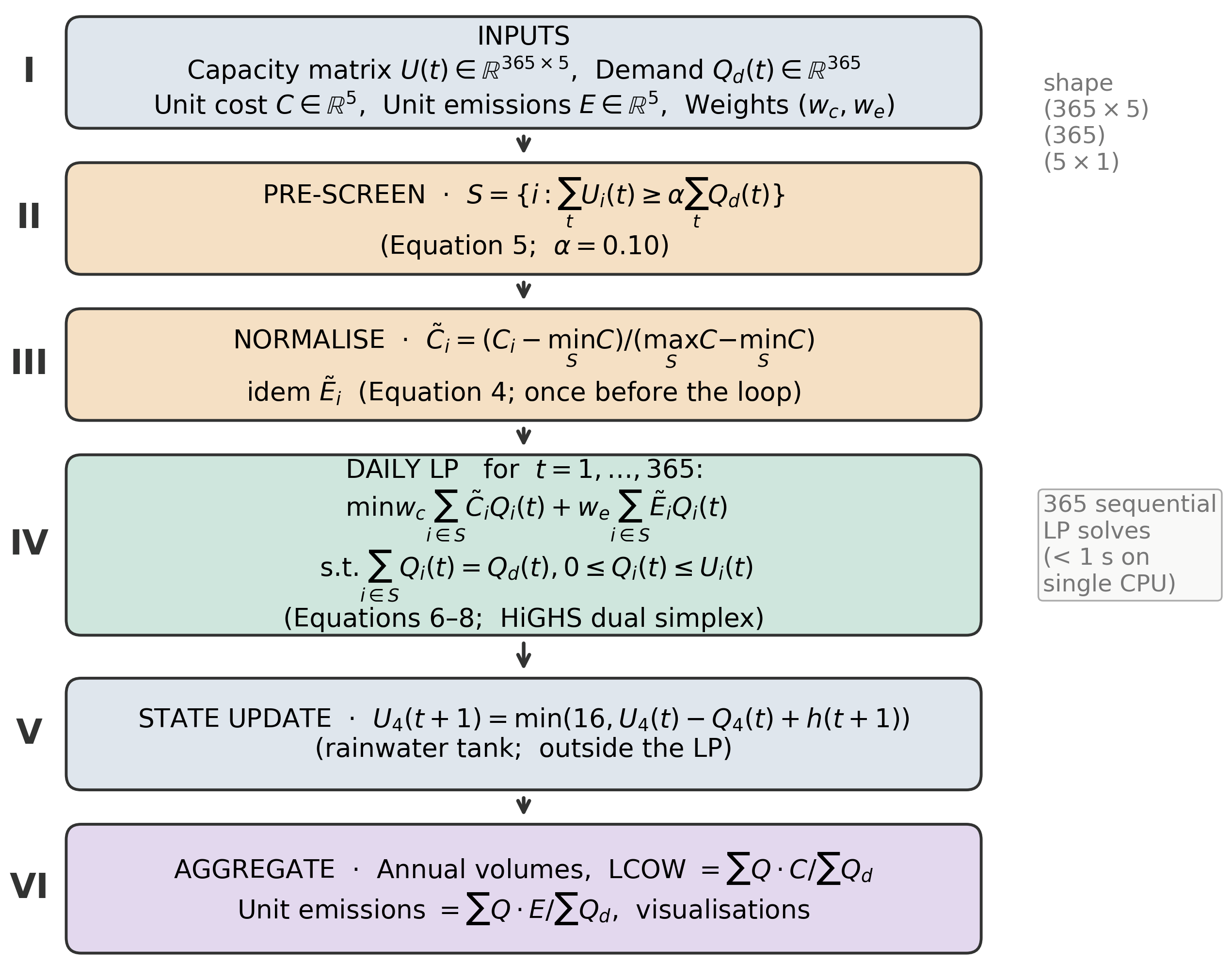
The 365 daily LPs are solved sequentially using SciPy’s ‘linprog’ solver with the HiGHS dual-simplex backend, in a Python 3 environment validated under Python 3.14.3, SciPy 1.17.1, NumPy 2.4.4 and pandas 3.0.2. Two CSV inputs feed the solver: ‘LP_alg/WaterProfiles_Modified.csv’, containing the 365 × 5 capacity matrix used for the reported results, and ‘Datasets/daily_water_demand_2021.csv’, containing the daily demand vector . The unit-cost and unit-emission constants and are encoded as Python lists at the top of the script and normalised once at start-up. A schematic of the solver flow is shown in Figure 2.
Stage I ingests the capacity matrix, the demand vector, the unit cost and unit emissions vectors and the scalarisation weights, with the data-shape annotations on the right edge confirming that the inputs match the LP solver expectations. Stage II applies the pre-screening filter of Equation (5) with the threshold = 0.10. Stage III performs the min–max normalisation of Equation (4) once before the daily loop; performing it inside the loop would re-normalise against the per-day capacity envelope rather than the source coefficients and is therefore explicitly avoided. Stage IV is the inner daily LP, solved with the HiGHS dual-simplex backend; the side annotation confirms that the 365 sequential solves complete under low load. Stage V updates the rainwater-tank state outside the LP—the only inter-day coupling in the formulation. Stage VI aggregates the daily allocations into the LCOW and unit-emissions diagnostics reported in Table 5 and Table 6.
Figure 2.
Algorithmic flow of the daily linear-programming solver, structured as six sequential stages (I–VI).
Two of the five capacity profiles are dynamic and require special handling outside the LP. The rainwater profile U4(t) is updated as a state carry-forward: the available rainwater volume on day is the previous day’s residual plus the day- harvest, capped at the 16 m3 tank limit; after each daily solution, the residual is updated and propagated to day + 1. The reuse profile U5(t) is treated as a static daily constant equal to the residual of the previous year’s water consumption, distributed uniformly across operational days; this deliberate simplification preserves linearity. A fully dynamic implementation that ties U5(t) to a fraction (≤0.6) of would be straightforward to plug in and is identified as future work.
Outputs from the daily solution are aggregated into yearly contribution vectors, used to compute the post-optimisation Levelised Cost of Water and unit-emissions metric, and visualised as stacked area charts (Figure 3) and contribution heatmaps (Figure 4). The pre-optimisation reference is the case in which the brewery satisfies the entirety of its 2022 demand from the municipal source alone, = , = 0 for ≠ 1.
3.8. Sensitivity-Analysis Design
The final methodological layer stresses the optimum against four perturbation families. The Balanced scenario is taken as the reference because it is the most managerially representative weighting. For all four sweeps, the optimisation is re-run from scratch on the perturbed inputs, with no exogenous cap on individual source contributions other than those imposed by the pre-screening filter (Equation (5)) and the per-day capacity constraint (Equation (8)).
3.8.1. Diversification Bounds
Equation (8) is augmented with an upper-share constraint, ≤ β · Q_d(t), with ∈ {1.00, 0.80, 0.50, 0.40, 0.25}. The reference scenario corresponds to = 1.00 (no diversification cap). Tightening forces the solver to spread the daily allocation across at least 1/ sources, simulating regulatory or risk-management policies that explicitly prevent over-reliance on any single source. The five values are chosen on a near-logarithmic grid that brackets both the lightly-binding (0.80) and the demand-infeasible (0.25) extremes.
3.8.2. Groundwater Capacity
The groundwater capacity vector is multiplied by a factor ∈ {0.4, 0.8, 1.0, 1.5, 2.0}, simulating aquifer depletion ( < 1) or relaxation of the conservative extraction policy ( > 1). For > 1, the daily share is allowed to exceed the reference solution: the absence of an upward saturation in this sweep is intentional and makes the asymmetry reported in Section 4.5.2 a true data-driven finding rather than an artefact of the bound.
3.8.3. River-Water Capacity
The river capacity vector is multiplied by a factor ∈ {0.4, 0.8, 1.0, 1.5, 2.0}, simulating prolonged drought or flood-augmented river flows. River-flow climate sensitivities of this magnitude are within the range projected for Mediterranean basins under RCP4.5 and RCP8.5 [53].
3.8.4. Grid Emission Factor
The Cretan grid emission factor (0.989 kg CO2eq kWh−1) is one of the most carbon-intensive grids in the European Union. To bound the generalisability of the headline emissions reduction, the unit-emissions vector is recomputed at three additional grid factors: 0.50 (typical southern-European mainland mix), 0.25 (current EU-27 average) and 0.10 (low-carbon mix consistent with high-renewable-penetration grids). The Balanced LP is re-solved at each grid factor and the resulting LCOW–emissions trade-off is plotted in Section 4.6.
For each variant, the LP is re-solved on the full 365-day horizon, and the resulting LCOW and unit emissions are recorded. Capacity percentages reported throughout the Results are evaluated against the calendar-year theoretical maximum (365 × the maximum daily withdrawal rate) for the river, groundwater and rainwater pathways. For reuse, which is by definition only available on operational days, the percentage is taken against the operational-day denominator (304 × 14.34 m3 d−1 ≈ 4360 m3 yr−1); the alternative 365-day denominator is not meaningful for a source whose capacity is zero on non-operational days.
4. Results
4.1. Pre-Optimisation Baseline
In the pre-optimisation configuration, the brewery sources its full annual demand of 5250 m3 from the municipal network, including the on-site RO polishing unit. The Levelised Cost of Water is 1.742 EUR m−3, and the unit emissions are 12.279 kg CO2eq m−3. These two values are used as the comparator for all subsequent scenarios.
4.2. Balanced and Cost-Focused Scenarios—Coincident Optima
Under the Balanced weighting (, ) = (0.65, 0.35) and the Cost-focused weighting (, ) = (0.90, 0.10), the LP returns numerically identical solutions. Both allocate the annual demand across three of the five sources. Rainwater is filtered out by the pre-screening rule (Equation (5)) because its 238.4 m3 annual harvest falls below the 525 m3 threshold (= 0.10 × 5250 m3), and reuse is excluded by the LP itself because its 2.050 EUR m−3 unit cost is uncompetitive once the emissions term carries 35% or less of the weight (Table 5). Groundwater dominates the solution at 3420.0 m3 yr−1 (83.3% of the calendar-year theoretical maximum, equivalently 100% of the 304-day operational cap), followed by the river at 1032.6 m3 (20.3%) and a residual municipal contribution of 797.4 m3 that fills demand on summer days when river flow is at zero, and the groundwater daily ceiling is binding. The exclusion of rainwater is therefore first an engineering-economic outcome rather than an optimisation result: its 5.382 EUR m−3 unit cost—the highest in the matrix, driven by the small 238.4 m3 annual harvest over which the equipment cost is amortised at 452 mm of local rainfall—keeps it uncompetitive even when admitted. A pre-screening-threshold sweep confirms this (Section 4.8.3): lowering α below the 0.045 eligibility cut-off re-admits rainwater to the eligible set, yet it still draws zero volume in every scenario because it is dominated on both cost and emissions. The framework can nonetheless incorporate rainwater whenever a larger catchment, a corporate-social-responsibility objective or an emergency-backup requirement raises its effective value, simply by relaxing α.
The aggregate metrics, total annual cost 6828.7 EUR, total annual emissions 38,203.1 kg CO2eq, LCOW 1.301 EUR m−3 and unit emissions 7.277 kg CO2eq m−3, translate, relative to the pre-optimisation baseline, to a 25.3% LCOW reduction and a 40.7% emissions reduction (Table 6). The cost reduction is the largest of the three scenarios, but the emissions reduction is smaller than under the Eco-friendly scenario because the cost-leaning weighting substitutes cheaper but more carbon-intensive groundwater for cleaner but more expensive river water on a substantial number of days. Throughout, four-significant-figure values are reported for reproducibility (Table 5 and Table 6); given the underlying input-data uncertainties, differences beyond the second significant figure should not be over-interpreted.
The coincident outcome of the Balanced and Cost-focused scenarios is the most structurally informative feature of the optimisation layer. After min–max normalisation across the eligible four sources, the cost ranking is groundwater < river < municipal < reuse, while the emissions ranking is river < groundwater < reuse < municipal. The cheapest source (groundwater) and the cleanest source (river) therefore lie on the same side of the cost–emissions plane, but groundwater wins on cost while river wins on emissions. With 35% weight on emissions (the Balanced setting), the cost-side advantage of groundwater more than compensates for its emissions handicap relative to river, so the LP places groundwater at its capacity ceiling and uses river only as a complement when groundwater alone cannot meet the daily demand. Pushing emissions weight from 0.35 to 0.10 (the Cost-focused setting) does not change the rank ordering of the per-source objective contributions, so the optimum is unchanged. The threshold emissions weight at which the optimum shifts to a river-dominant solution lies between 0.35 and 0.90; an analytical estimate (using the normalised coefficients of Section 3.5) places it at approximately ≈ 0.43.
4.3. Eco-Friendly Scenario
Reversing the weights to (, ) = (0.10, 0.90) produces a structurally different optimum. Groundwater drops from 3420 to 2542.6 m3 yr−1 (61.9%), the river rises from 1032.6 to 1910.0 m3 yr−1 (37.5%), reuse enters the solution at 668.3 m3 yr−1 (15.3%), and the residual municipal contribution drops from 797.4 to 129.1 m3 (Table 5).
The aggregate metrics are LCOW 1.405 EUR m−3, unit emissions 5.930 kg CO2eq m−3, total annual cost 7377.6 EUR and total annual emissions 31,134.6 kg CO2eq. Relative to the baseline, this is a 19.3% LCOW reduction and a 51.7% emissions reduction (Table 6), the largest emissions saving of the three scenarios, achieved at a 6-percentage-point cost penalty relative to the Balanced/Cost-focused optimum. The eco-friendly weighting therefore reveals a true cost–emissions trade-off internal to the source matrix: the firm gives up 0.105 EUR m−3 of LCOW reduction in exchange for 1.347 kg CO2eq m−3 of additional emissions reduction.
The intra-year heatmap of contributions for the Eco-friendly scenario (Figure 4) reveals a coherent strategic pattern. River water is the dominant source from January through April and from November through December, when its capacity exceeds the daily demand on most days. Groundwater operates as a near-constant base load through the summer and early autumn months when river flow falls to zero. Reuse fills the gap during summer when neither river nor groundwater alone meets the demand, and municipal water is deployed only on the rare days when the combined capacity of the three other sources is insufficient.
Figure 3.
Daily allocation, monthly aggregation, and annual share of each source under the three managerial scenarios.
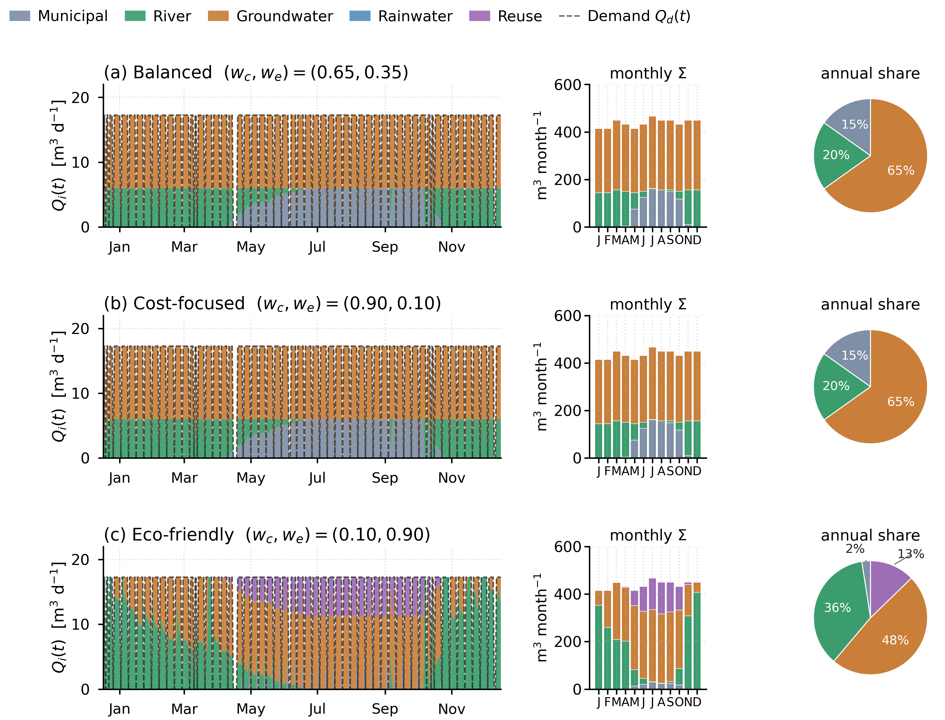
Each row corresponds to one scenario (Balanced, Cost-focused, Eco-friendly). The left column plots the stacked daily allocations across the 365-day horizon, with the dashed black line marking the daily demand; the visual identity of Figure 3a,b confirms the coincident-optima finding reported in Section 4.2. The middle column re-aggregates the same daily values into twelve monthly volumes, summarising the seasonal substitution pattern: under Figure 3a,b the source mix is largely time-invariant, whereas under Figure 3c the river dominates winter months and groundwater + reuse take over in summer. The right column condenses the annual totals into a pie chart that reports each source’s share of the 5250 m3 yr−1 delivered demand. The threefold representation—daily, monthly, annual—makes the interaction between hydrological seasonality and managerial weighting legible at three temporal scales without any change of underlying data.
Figure 4.
Per-source daily allocation under the Eco-friendly scenario.
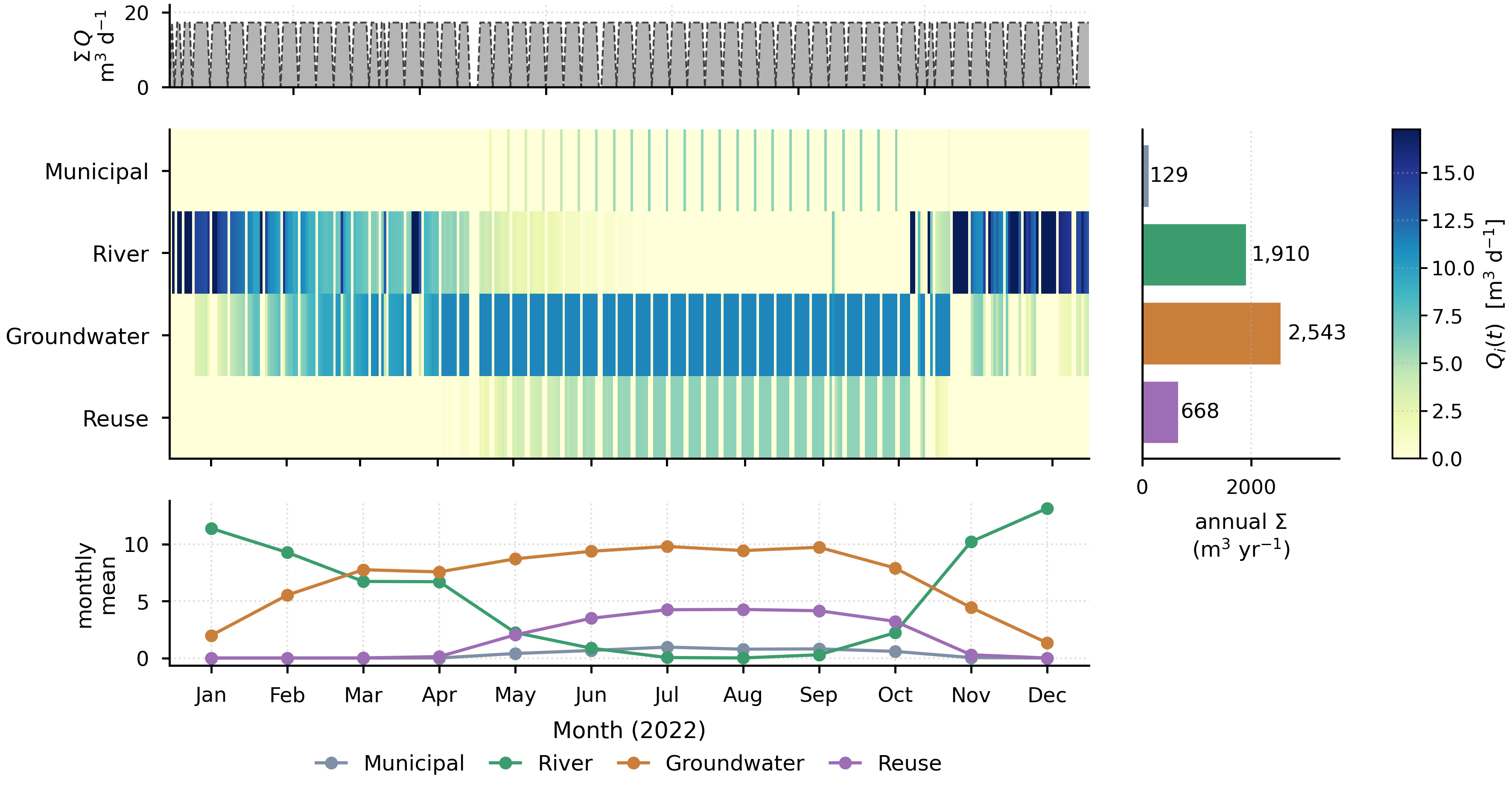
Figure 4 is plotted as a heatmap across the 365 days of 2022, with three marginal aggregates that together summarise the spatial, temporal and quantitative structure of the optimum. The top marginal trace plots the total daily delivered volume Σ against the dashed-black demand line, confirming that the LP exactly satisfies demand on every operational day (the dips correspond to the 62 non-operational days). The main heatmap encodes the allocation matrix as colour intensity, with rows ordered by typical seasonal contribution; rainwater is omitted because it is filtered out by Equation (5). The right-hand horizontal-bar marginal reports each source’s annual total in m3 yr−1 alongside the heatmap, providing the cross-source comparison that the heatmap alone cannot. The bottom panel plots the monthly mean of each source’s allocation as small multiples on a single set of axes; the seasonal handover between river (winter dominant, peaking at 11 m3 d−1 in December) and groundwater + reuse (summer dominant, peaking at 8–9 m3 d−1 in July–August) is the operational signature of the framework’s emissions-minimising strategy.
4.4. Cross-Scenario Comparison
A side-by-side reading of Table 5 and Table 6 produces three observations. First, both LCOW and unit-emissions curves drop monotonically away from the pre-optimisation baseline; no scenario worsens either metric. Second, the cost–emissions trade-off is internal to the optimisation rather than imposed by the data: the Balanced/Cost-focused scenarios give up 11 percentage points of emissions reduction to gain 6 percentage points of cost reduction relative to the Eco-friendly case. Third, the coincidence of the Balanced and Cost-focused optima implies that managerial weights anywhere in the cost-leaning range ≲ 0.43 deliver the same supply mix; an aggressive emissions weight unlocks an emissions-leaning optimum, and the continuous weight sweep reported in Section 4.7 reveals an intermediate regime between the two named ones. The cost–emissions trade-off across scenarios is depicted in Figure 5.
Figure 5.
Pareto frontier of (LCOW, unit emissions) outcomes across a continuous weight sweep ∈ [0, 1] in 41 steps.
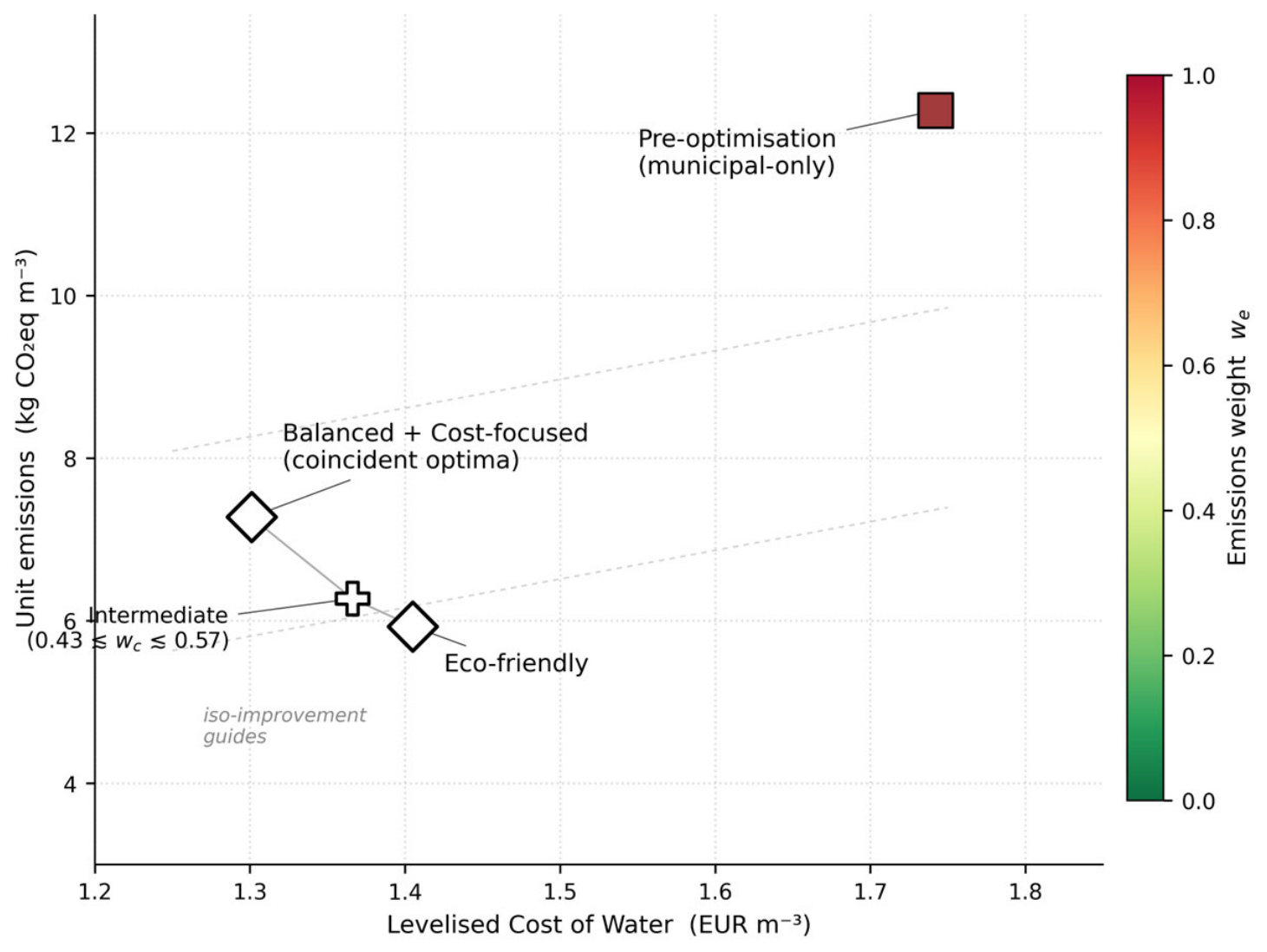
In Figure 5, the three named managerial scenarios and the pre-optimisation baseline are overlaid. The colour of each scattered point encodes the emissions weight = 1 − (red for emissions-leaning, green for cost-leaning), so the Pareto curve is also a one-dimensional weight-trajectory map. The diamond markers identify the two distinct optima under the studied weight pairs: a coincident point at (1.301, 7.277) shared by the Balanced and Cost-focused scenarios, and a single Eco-friendly point at (1.405, 5.930). The vertical dotted line marks the analytical pivot weight at ≈0.43, where the LP optimum jumps discontinuously between the two regimes, a consequence of the polytope geometry rather than a smooth interpolation. The dashed-grey iso-improvement guides indicate loci of equivalent joint reduction in LCOW and unit emissions relative to the municipal-only baseline. The square red marker fixes the pre-optimisation reference at (1.7421, 12.279) and visualises the magnitude of the joint improvement that the framework achieves at any non-zero weight pair on the frontier.
4.5. Sensitivity Analysis: Bounds and Capacity Perturbations
4.5.1. Diversification Bounds
Tightening the per-source share constraint progressively raises both LCOW and unit emissions (Figure 6a, Table 7). At = 0.80, the LCOW remains identical to the reference (1.301 EUR m−3), and unit emissions are unchanged, because the reference solution itself never exceeds an 80% per-source share on any operational day. At = 0.50, the LCOW rises to 1.380 EUR m−3 (+6.1% above reference) and unit emissions drift up by less than 1%. From = 0.40 onwards, the system pays a measurable price for diversification: the LCOW rises to 1.466 EUR m−3, and the system can no longer satisfy demand on every operational day (annual delivered volume falls to 5183 m3, a 1.3% shortfall). At = 0.25, the shortfall reaches 14% (delivered volume 4499 m3) and the LCOW reaches 1.601 EUR m−3. The 0.25-bound case fails because no single source may deliver more than a quarter of the daily demand (4.32 m3), so feasible operation requires at least four simultaneously available sources with sufficient aggregate capacity. On dry summer days, river capacity is below this cap, and rainwater is excluded by Equation (5), leaving too little capped capacity to satisfy demand.
Table 7.
Sensitivity analysis: LCOW and unit emissions for each variant.
The interpretation is policy-relevant. A diversification ceiling up to roughly = 0.80 is cost-neutral in this case; from there to = 0.50 it imposes a small cost penalty but no demand shortfall; below = 0.50 the curve turns sharply upward, and the system begins to fail demand on stressed days. The framework therefore identifies ≈ 0.80 as a site-specific starting point for a regulatory or risk-management ceiling, capturing diversification without measurable cost or emissions penalty in the tested source matrix.
4.5.2. Groundwater-Capacity Perturbations
Multiplying by = 0.4 raises the LCOW to 1.511 EUR m−3 and unit emissions to 7.682 kg CO2eq m−3 (Figure 6b, Table 7); both deteriorate relative to the reference. At = 0.8, the deterioration is mild but measurable. Raising above 1.0, in contrast, lowers the LCOW further (because the optimum substitutes cheaper groundwater for river and municipal water on days when river flow is weak), but the unit emissions rise slightly because the substitution is towards a more carbon-intensive source. At = 2.0, the LCOW reaches 1.131 EUR m−3, the standalone groundwater LCOW, indicating that the LP has converged on a near-monoculture solution.
The asymmetry between the < 1 and > 1 regimes is informative. A firm whose aquifer remains healthy enjoys a small additional LCOW gain at the cost of a small emissions penalty; a firm whose aquifer depletes to = 0.4 pays a substantial cost-and-emissions penalty. Aquifer protection therefore behaves like an option whose downside is large and whose upside is modest, an asymmetry that justifies a precautionary extraction policy in regions of documented over-extraction. Read as a real option, the value of preserving aquifer headroom is sharply asymmetric—large downside protection for only a modest upside cost—which strengthens the case for the precautionary groundwater-governance regimes increasingly advocated for stressed Mediterranean basins; the shadow-price analysis of Section 4.8.5 attaches a direct monetary value to that headroom.
4.5.3. River-Capacity Perturbations
The river-capacity sweep produces the smallest cost effect of the three sweeps but the largest emissions effect (Figure 6c, Table 7). LCOW barely moves across ∈ [0.4, 2.0]; unit emissions, by contrast, fall from 7.878 kg CO2eq m−3 at = 0.4 to 7.073 at = 2.0. The pattern reflects the structural fact that river OSRO is the cleanest source by a factor of four but only the second-cheapest: extra river availability lets the LP substitute river for groundwater on the emissions side, but at almost no cost penalty because the two unit costs are within 35% of one another.
The two-tone behaviour is informative. Under a future climate that increases river flows (a possible outcome for some Mediterranean sub-regions during the rainy season), the system is well-positioned to lower its emissions at negligible cost. Under a drought future that decreases river flows, the cost penalty is small, but the emissions penalty is real: the system must substitute groundwater for river, paying a structural carbon cost.
Figure 6.
Sensitivity composite for the Balanced scenario, structured as a 2 × 3 grid of complementary perspectives plus a parameter-influence ranking.
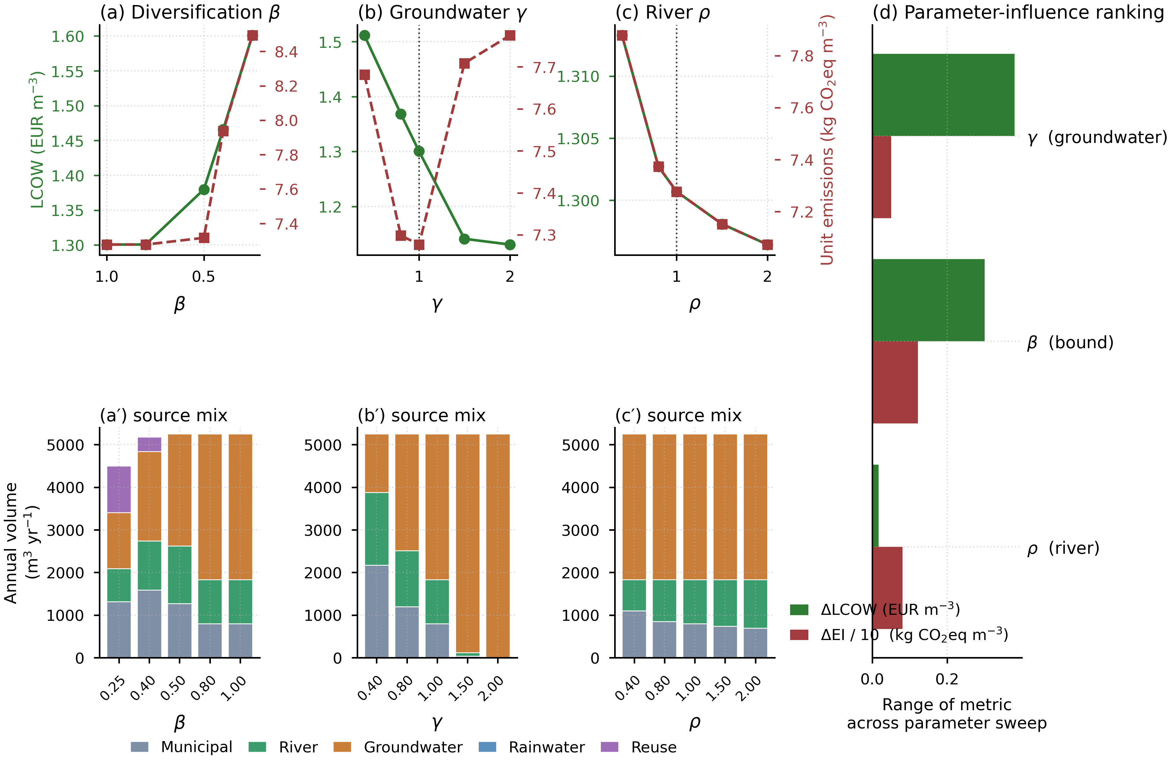
The top row (Figure 6a–c) plots LCOW (green, left axis) and unit emissions (red, right axis) against the three perturbation parameters: the per-source share cap with the axis inverted so that tighter constraints sit to the right Figure 6a, the groundwater-capacity multiplier with the reference = 1 marked by a vertical dotted line Figure 6b, and the river-capacity multiplier with the same convention Figure 6c. The bottom row (Figure 6a′–c′, stacked beneath their corresponding top panels) shows the source mix at every perturbation level as stacked bars, summarising the substitution mechanism that drives each metric trend. Figure 6d on the right is a tornado plot ranking the three parameters by the range of LCOW and unit emissions they induce across the swept range; and dominate the LCOW range while dominates the emissions range, consistent with the structural role each parameter plays in the LP geometry. The composite layout makes it possible to read each sensitivity at three levels in parallel: the aggregate metric trend, the underlying source-mix substitution, and the relative parameter influence.
4.6. Generalisability: Parametric Sweep over the Grid Emission Factor
The headline emissions reduction reported in Section 4.2, Section 4.3 and Section 4.4 reflects, in part, the unusually high carbon intensity of the Cretan-island electricity grid (0.989 kg CO2eq kWh−1). To bound the generalisability of the result, the Balanced LP is re-solved with the unit-emissions vector recomputed at three additional grid factors: 0.50 kg CO2eq kWh−1 (typical southern-European mainland mix), 0.25 (current EU-27 average) and 0.10 (low-carbon mix). All other inputs are held constant.
Two structural findings emerge (Figure 7). First, the cost-side optimum is independent of the grid factor by construction: the Balanced LCOW remains at 1.301 EUR m−3 across the four grids. Second, the absolute emissions-side benefits scale roughly linearly with the grid factor, but the fractional reduction relative to the municipal-only baseline is preserved at approximately 41% across all grids tested. The reason is that both the baseline and the alternative trains share the same grid, so a less carbon-intensive grid attenuates the absolute emissions of all five sources by the same factor and leaves the ratio invariant. The emissions-reduction ratio therefore transfers to less carbon-intensive grids under the assumption that all treatment trains draw from the same grid and that non-electricity emissions remain second-order, even if the absolute kg CO2eq m−3 reductions reported as the headline numbers attenuate proportionally.
A practical corollary: industries operating on grids approaching the EU-27 average of 0.25 kg CO2eq kWh−1 should expect an absolute emissions reduction of roughly 1.27 kg CO2eq m−3 rather than the 5.00 kg CO2eq m−3 obtained on the Cretan grid. That remains a non-trivial saving in absolute terms and is proportionate to the grid’s residual carbon intensity. The headline 41–51% fractional reductions, by contrast, are structural properties of the source matrix and transfer beyond the case study. The transferability claim is deliberately confined to these fractional reductions and to the framework’s diagnostics; the optimal supply-mix structure itself—here groundwater-dominant—is a property of the local cost-and-emissions matrix and need not carry over. On a site where, for example, river water was both the cheapest and the cleanest source, the pivot weights of Section 3.6.4 would simply be recomputed from the new coefficients, and the same machinery would identify a river-dominant optimum.
Figure 7.
Generalisability sweep over the regional grid emission factor, separated into absolute (a) and fractional (b) emissions metrics across all three managerial scenarios.
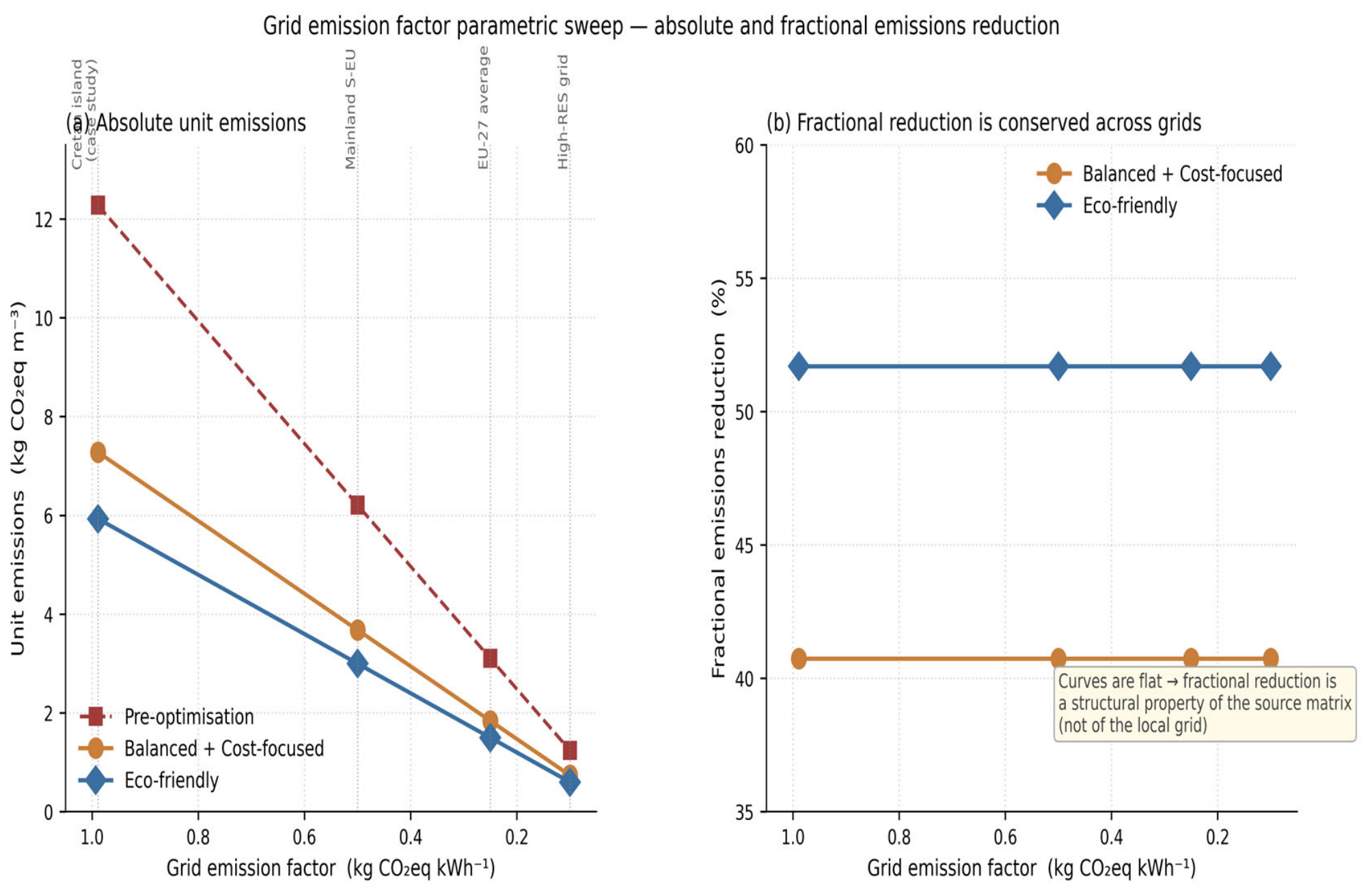
Figure 7a plots unit emissions in absolute kg CO2eq m−3 for the pre-optimisation baseline, the coincident Balanced/Cost-focused optimum, and the Eco-friendly optimum as the grid factor decreases from 0.989 (Cretan island) through 0.50 (typical southern-European mainland), 0.25 (EU-27 average) and 0.10 (high-renewable-penetration grid). The vertical guides mark the four reference grid factors. All three traces decline approximately linearly with the grid factor; the curves are non-crossing because every train shares the same grid. Figure 7b plots the fractional emissions reduction relative to the pre-optimisation baseline. The two scenario curves are essentially flat at 40.7% (Balanced/Cost-focused) and 51.7% (Eco-friendly) across the four grid factors tested, demonstrating that the fractional reduction is a structural property of the source-cost-and-emissions matrix rather than of the local grid. The flat curves are the central generalisability claim of the framework: a firm operating on a less carbon-intensive grid still recovers the full fractional improvement, even though the absolute kg CO2eq m−3 saving attenuates proportionally with grid factor.
4.7. Continuous Weight Sweep
The three managerial scenarios are discrete samples of a continuous weight space. To trace the full geometry of the optimum across that space, the LP is re-solved at 41 evenly-spaced ∈ [0, 1] values in steps of 0.025; the resulting source mix and aggregate metrics are plotted in Figure 8.
Figure 8.
Continuous weight sweep across ∈ [0, 1] in 41 steps.
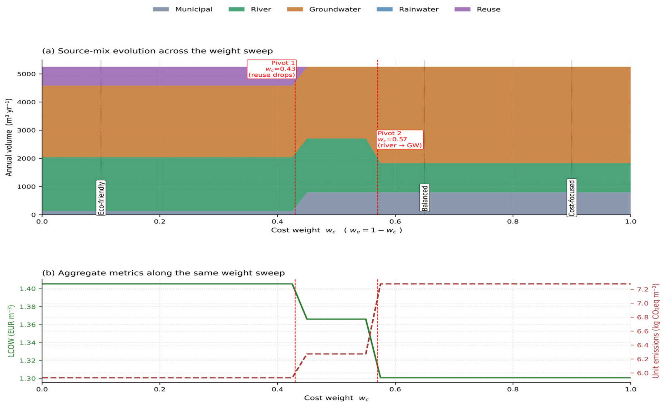
Figure 8a plots the annual contribution of each source as a stacked area against the vertical dotted lines, mark the three named scenarios (Eco-friendly at = 0.10, Balanced at = 0.65, Cost-focused at = 0.90). The continuous sweep reveals two pivot weights at which the LP optimum jumps discontinuously between vertex solutions: a first pivot near ≈ 0.43 at which reuse drops out of the mix, and a second pivot near ≈ 0.57 at which the river-vs-groundwater preference flips. Figure 8b plots the corresponding LCOW (green, left axis) and unit emissions (red, right axis) on the same horizontal axis. Both metrics are step functions, holding approximately constant within each weight regime and switching sharply at the two pivots, mirroring the discrete vertex transitions of the underlying convex polytope.
The separated weight-sweep panels confirm three claims that the discrete-scenario figures could only suggest. First, the source mix is piecewise-constant in the weight, with three dominant regimes separated by the two pivots: an emissions-leaning regime ( ≲ 0.43) in which river, groundwater and reuse share the supply with reuse contributing about 670 m3 yr−1; an intermediate regime (0.45 ≲ ≲ 0.55) in which reuse has dropped out and the lost share is absorbed by municipal water at the same river/groundwater envelope (LCOW = 1.366 EUR m−3, EI = 6.27 kg CO2eq m−3); and a cost-leaning regime ( ≳ 0.57) in which groundwater saturates the cap, river contributes only its lowest-cost portion, and reuse remains absent. Second, the aggregate metrics LCOW and unit emissions move in synchrony with the source mix and trace a two-step ladder, with LCOW values 1.405 → 1.366 → 1.301 EUR m−3 and unit emissions 5.93 → 6.27 → 7.28 kg CO2eq m−3 across the three regimes. Third, the three named scenarios populate only two of the three vertices: Balanced and Cost-focused both fall inside the cost-leaning regime; only the Eco-friendly weight lies on the emissions-leaning side of the first pivot, and none of the three named scenarios samples the intermediate regime. The continuous sweep therefore reframes the original three-scenario report as a sample of two of three distinct optima and motivates the recommendation in Section 5.4 that managerial weight selection should be informed by the firm’s location relative to the two pivots rather than by the percentage labels alone.
4.8. Additional Robustness Analyses and Solution-Method Validation
This subsection adds a set of further analyses that bound the parameter uncertainty raised in the review and validate the solution method. Each re-solves the same daily LP on perturbed inputs; the discount-rate, recovery and demand-profile results are collected in Table 8.
Table 8.
Additional robustness analyses for the Balanced scenario: optimised LCOW and unit emissions under discount-rate, reverse-osmosis-recovery and demand-profile perturbations. Reference rows reproduce the baseline Balanced optimum.
4.8.1. Discount-Rate Sensitivity
Holding the cost decomposition of Section 3.3 fixed, the capital-recovery factor in Equation (1) is re-evaluated at r ∈ {0.05, 0.08, 0.10, 0.12, 0.15}, the per-source unit costs are re-derived, and the Balanced LP is re-solved (Figure 9a, Table 8). The optimised LCOW rises monotonically from 1.196 EUR m−3 at r = 0.05 to 1.439 EUR m−3 at r = 0.15, an −8% to +11% band around the 1.301 EUR m−3 reference. Below r ≈ 0.08, the discount rate also has a structural effect: the cheaper river-OSRO capital cost pulls the optimum across the first weight pivot into the river-leaning intermediate regime, lowering unit emissions from 7.277 to 6.272 kg CO2eq m−3. The groundwater-led diversified structure is preserved across the whole range, so the headline conclusions are robust to the assumed cost of capital, while a lower discount rate makes the cleaner river source more competitive.
4.8.2. Reverse-Osmosis Recovery Sensitivity
The 100% recovery idealisation of Section 3.2 is relaxed with a transparent first-order model: at recovery η, each RO stage processes 1/η m3 of feed per m3 of permeate, so its electricity intensity scales by 1/η and a brine-disposal charge of c_b(1/η − 1) EUR m−3 is added, with a central c_b = 0.5 EUR m−3 (range 0.3–1.0). The unit-cost and unit-emissions vectors are re-derived and the Balanced LP re-solved (Figure 9b, Table 8). At a representative η = 0.75, the per-source unit costs rise by 13.9% (river OSRO), 29.1% (groundwater) and 12.3% (reuse), and the optimised Balanced LCOW rises from 1.301 to 1.631 EUR m−3 (+25%); at η = 0.60, it reaches 1.895 EUR m−3 (+46%). Groundwater carries the largest per-source penalty because it is the most RO-energy-intensive train, yet it remains the cheapest source, and the diversified groundwater-led optimum survives at every recovery level tested. Varying c_b over 0.3–1.0 EUR m−3 moves the η = 0.75 LCOW only within 1.564–1.797 EUR m−3 and does not change this conclusion.
Figure 9.
Discount rate and reverse osmosis recovery sensitivity of the Balanced optimum. (a) Optimised LCOW (green) and unit emissions (red) across discount rates r from 0.05 to 0.15; the step in unit emissions at r ≤ 0.08 marks the optimum crossing the first weight pivot into the river-leaning regime. (b) Increase in per-source RO-train unit cost (left axis: river OSRO, groundwater RO, reuse RO) and optimised Balanced LCOW (right axis) as the RO recovery rate η falls from 1.0 to 0.6.
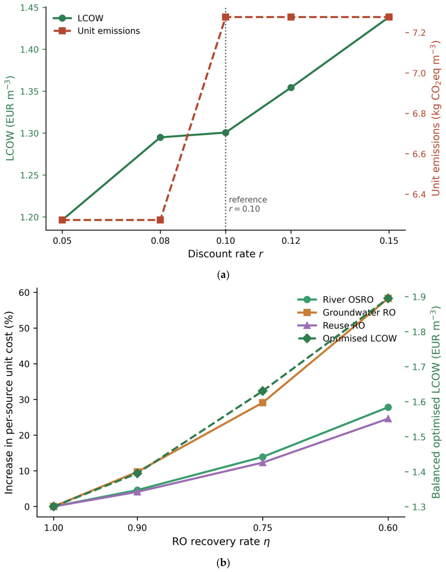
4.8.3. Pre-Screening Threshold and Demand Profile
Two structural assumptions are stressed. First, the pre-screening threshold is swept downward: lowering α below the eligibility cut-off of 0.045 (= 238.4 ÷ 5250) re-admits rainwater to the eligible set, but rainwater still draws zero volume in every scenario because its unit cost (5.382 EUR m−3) and unit emissions (10.001 kg CO2eq m−3) are both dominated. The exclusion of rainwater is therefore an economic outcome, not an artefact of the α = 0.10 setting. Second, the uniform daily demand is replaced by two seasonal profiles carrying the same 5250 m3 annual total (Table 8): a summer-peaked craft-brewery profile and a winter-peaked profile. The summer-peaked profile raises the Balanced LCOW to 1.327 EUR m−3 and unit emissions to 8.531 kg CO2eq m−3—demand concentrates when river flow is at its seasonal minimum, forcing more municipal water—while the winter-peaked profile lowers them to 1.281 EUR m−3 and 6.281 kg CO2eq m−3. Both shifts are smaller than the spread between the named scenarios and leave the groundwater-led ranking intact, so the uniform-demand simplification is directionally transparent rather than results-determining.
4.8.4. Equivalence of the Weighted-Sum and ε-Constraint Frontiers
To confirm that the weighted-sum scalarisation does not miss supported Pareto points, the allocation problem is re-solved as a single aggregate ε-constraint program—minimise total cost subject to total emissions ≤ ε—swept across the achievable emissions range (Figure 10). The ε-constraint frontier coincides with the weighted-sum solutions at every vertex, sharing the identical endpoints (1.301 EUR m−3, 7.277 kg CO2eq m−3) and (1.405 EUR m−3, 5.930 kg CO2eq m−3) and passing through the same intermediate vertex (1.366 EUR m−3, 6.27 kg CO2eq m−3). Because the feasible set is a convex polytope, every Pareto-optimal point is supported, so the two methods are equivalent here; the ε-constraint formulation would become necessary only if a future non-convex extension introduced non-supported points (Section 5.5, L7).
Figure 10.
Equivalence of the weighted-sum and ε-constraint Pareto frontiers. The grey curve is the ε-constraint frontier (minimise cost subject to an emissions cap); the markers are the 41 weighted-sum solutions, shaded by cost weight w_c. Both recover the identical supported vertices, including the intermediate regime.
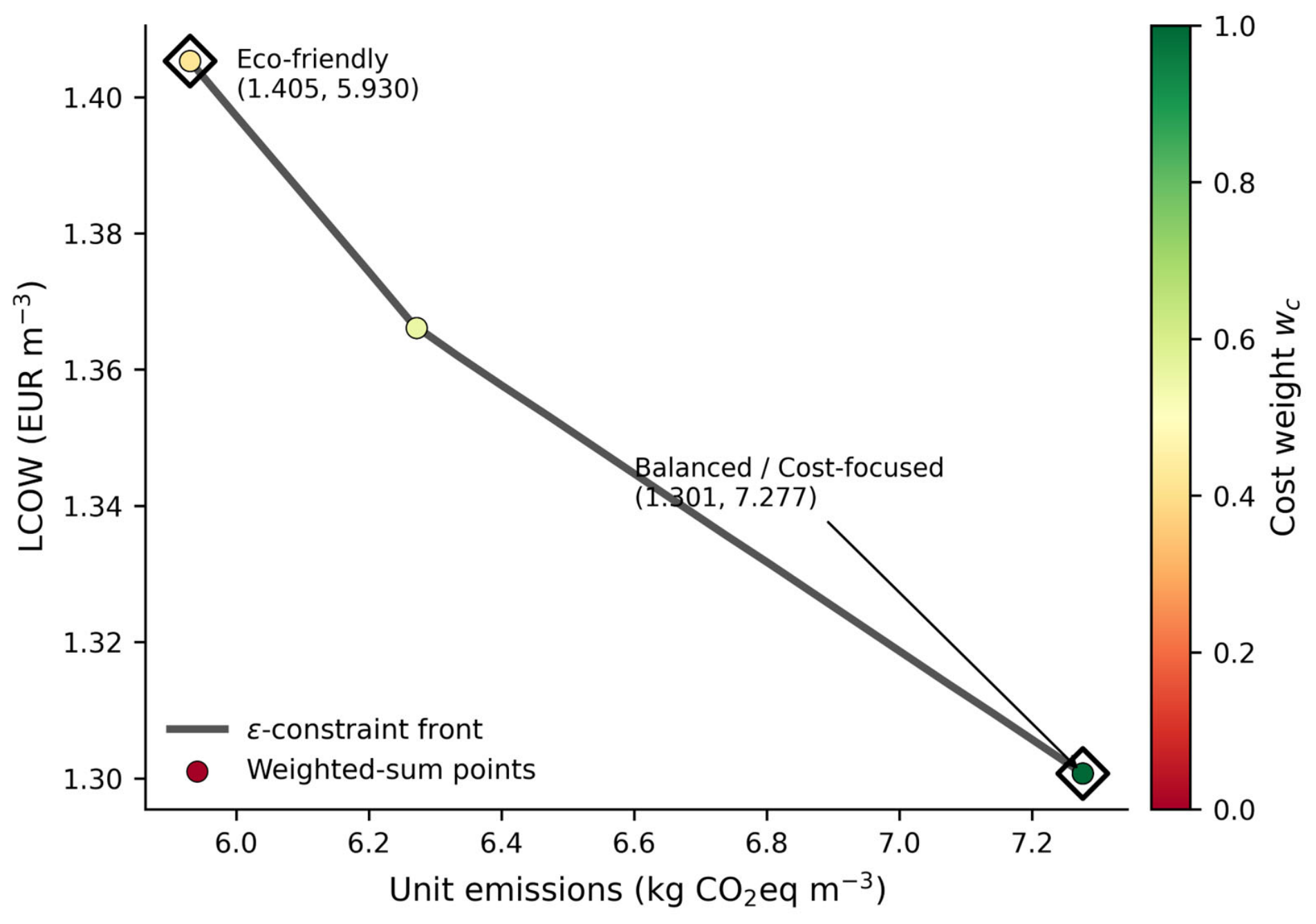
4.8.5. Shadow-Price Profiles
The daily LP duals are extracted directly from the HiGHS solver and reported here rather than only interpreted (Figure 11). The demand-constraint dual—the marginal cost of one additional cubic metre of demand—equals the river-OSRO LCOW (1.522 EUR m−3) through the winter months when river flow is abundant and rises to the municipal LCOW (1.742 EUR m−3) through May–August, when river flow falls to zero, and groundwater is capacity-bound, exactly the seasonal price signal anticipated in Section 3.6.5. The groundwater-capacity dual is positive on every operating day, peaks in summer, and summed across the operating year equals 154.7 EUR yr−1 per additional m3 d−1 of groundwater capacity—within 3% of the finite-difference proxy of Section 3.6.5. This dual is the quantitative answer to whether it is worth deepening the well or enlarging the abstraction permit, and the seasonal demand dual is the per-day signal a coupled supply–demand extension would target.
Figure 11.
Seasonal profile of the LP shadow prices for the Balanced scenario. The demand-constraint dual (line, left axis) tracks the river-OSRO LCOW (1.522 EUR m−3) in winter and the municipal LCOW (1.742 EUR m−3) in summer; the groundwater-capacity dual (bars, right axis) is positive on every operating day and peaks in summer. Summed over the operating year it equals 154.7 EUR yr−1 per additional m3 d−1 of groundwater capacity.
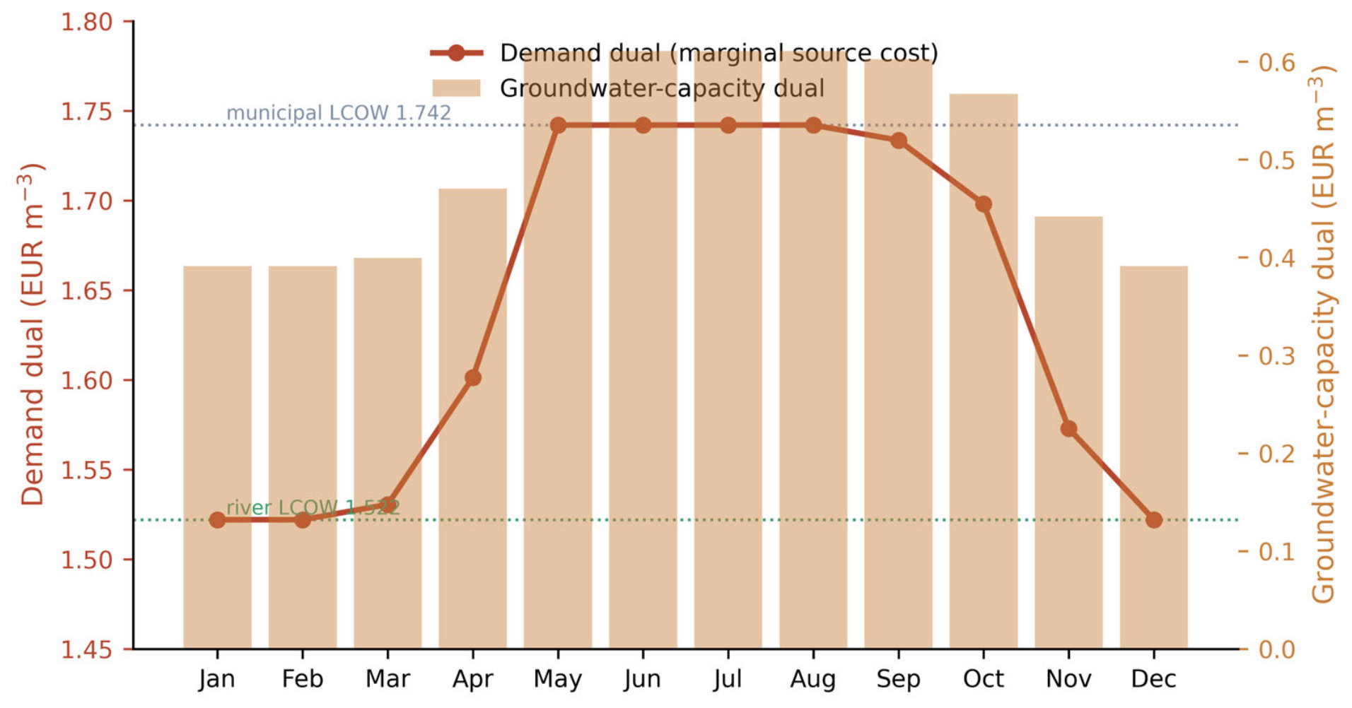
4.8.6. Solution-Method Efficiency
On a single CPU core, each daily LP solves in approximately 1.6 ms, a full 365-day scenario in about 0.5 s, and the complete suite—three scenarios, the nineteen sensitivity variants, the discount, recovery and demand-profile sweeps and the 41-step weight sweep—in well under a minute. For this convex problem, a population-based metaheuristic such as NSGA-II would, at best, reproduce the same vertex optimum while requiring Monte-Carlo replication and wall times of minutes per scenario, and—decisively—would not return the shadow-price duals of Section 4.8.5. The deterministic LP therefore dominates on speed, reproducibility and the governance information it yields.
5. Discussion
5.1. Asymmetry Between Cost and Emissions Weights
The most structurally informative result of the optimisation layer is the coincidence of the Balanced and Cost-focused optima. The two share the same vertex of the feasible polytope because, after min–max normalisation, the cost-side objective contributions of groundwater and river differ by enough that even a 35% emissions weight cannot reverse the cost-side ranking. Only at an emissions weight above ≈ 0.43 does the optimum shift towards a river-and-reuse-heavy mix. The implication is that, in the present source matrix, mild-to-moderate cost preference and aggressive cost preference are equivalent in their effect on the supply mix, whereas mild-to-moderate emissions preference is insufficient to alter the mix at all.
A 65/35 weight implements a cost-driven optimum, not a balanced one—the emissions weight is too low to bind, so the manager who sets weights at that level is in effect choosing the cost-minimising mix. Reaching the emissions-optimal mix requires an aggressive emissions weight (≥0.45), which industrial decision-makers may regard as politically uncomfortable when phrased as such, but which costs only 0.105 EUR m−3 in LCOW relative to the cost-optimum: a 6% cost penalty buys an additional 11% emissions reduction. This is the central managerial warning of the study: a nominally balanced weighting can silently implement a cost-driven decision whenever the cost and emissions vectors are sufficiently aligned. The analytic pivot calculation of Section 3.6.4 should therefore be treated as a mandatory pre-check—computed from the local source coefficients before any weight is reported—rather than as an after-the-fact diagnostic.
The structural lesson generalises beyond the case study. In any multi-source water system, the alignment between cost and emissions vectors should be checked explicitly before reporting a “trade-off” as inherent. The cost-and-emissions matrix in Table 4 is one specific arrangement, not a universal property of multi-origin systems; on a different matrix the Balanced and Eco-friendly weights might produce coincident optima instead.
5.2. Diversification as a Resilience Strategy
The diversification-bounds sensitivity (Section 4.5.1) makes the case for diversification quantitative. Up to ≈ 0.80, a per-source cap leaves both LCOW and emissions identical to the reference. From = 0.50 onwards, the LCOW rises monotonically, and the system begins to fail the daily demand. Diversification is best framed as a band rather than a corner: a moderate per-source ceiling can reduce over-reliance at negligible cost, while an aggressive cap forecloses the very flexibility it nominally promotes.
The river-capacity sensitivity (Section 4.5.3) reinforces the same conclusion from a different angle. The fact that the system can substitute reuse and groundwater for missing river flow allows it to absorb a 60% river-flow shock with only a 0.012 EUR m−3 LCOW penalty (Table 7). Without the reuse train in the active source mix, that absorption capacity would not exist. Diversification therefore offers two conceptually different goods: a cost-and-emissions optimum within nominal conditions, and a resilience reserve for stressed conditions.
5.3. Benchmarking and Positioning Within Operations-Research and Industrial-Cluster Decision Support
A direct numerical comparison places the present results against published industrial water-treatment benchmarks. The 1.301–1.405 EUR m−3 post-optimisation LCOW range is meaningfully below the 1.80 EUR m−3 value reported by Verhuelsdonk et al. [29] for full-scale brewery wastewater reuse alone, and competitive with the brewery-effluent membrane-treatment range of 1.5–2.5 EUR m−3 documented by Holloway et al. [25], Tay et al. [26] and Toran et al. [28]. The diversification framework lowers the blended cost below what any single alternative source could deliver on its own because the framework draws each source from its cheapest range and combines them according to the marginal cost of demand satisfaction. The 19–25% reduction is therefore not a benefit of any one treatment technology, but a benefit of integration—and the integration in question is precisely the cluster-level coordination across multiple supply trains.
The framework is also consistent with the broader process-systems-engineering literature on industrial water networks. The classical water-pinch and water-network synthesis methods, originating with the targeting and design heuristics of Wang and Smith [60] and consolidated in the textbook treatment of El-Halwagi [61] and the comprehensive review by Foo [62], optimise the internal reuse network within a single industrial site. The same lineage extends naturally into the explicitly multi-objective design of eco-industrial parks reviewed by Boix et al. [72], where the LP/MILP kernel coordinates resource flows across multiple co-located firms. The classical methods treat freshwater as a single input; the eco-industrial-park literature opens up the multi-firm cluster, but at the level of a network of plants. The framework developed here operates at a complementary intermediate layer, optimising the mix of imports into a single industrial site given a known internal demand, with the same LP-and-duality machinery that the cluster literature uses. A natural extension would couple three loops. The innermost loop performs water-pinch synthesis on the brewery’s internal water network. The intermediate loop is the multi-source LP developed here, supplying the internal network’s freshwater nodes. The outer loop opens an EIP-style coupling with neighbouring industrial sites along the cluster’s water and effluent flows.
Methodologically, the framework belongs to the operations-research tradition of weighted-sum multi-objective Linear Programming, with closed-form pivot derivation (Section 3.6.4) and shadow-price diagnostics (Section 3.6.5) that mirror the way decision-support systems for energy procurement, microgrid dispatch and industrial-cluster coordination are typically built [59,60,61,62,72,73]. The min–max normalisation adopted in Equation (4) follows the canonical recommendation for bounded-range physical coefficients in multi-objective programming [36], where z-score normalisation would require a probability distribution that the engineering coefficients do not have. The cost coefficients of Table 4 already embed the local energy price; the emissions coefficients embed the local grid factor; so the framework is, by construction, a water–energy nexus tool at the boundary between the brewing line and its external utilities, structurally identical to the LP kernels deployed for nearly Zero Energy Port and microgrid dispatch design where heterogeneous supply trains (grid, photovoltaics, storage, hydrogen) are coordinated by the same weighted-sum machinery [74]. Coupling the framework with a brewery-side energy procurement model—on-site photovoltaic generation, demand-side flexibility, electricity-tariff timing—or with the parallel energy supply trains of an industrial cluster would convert the supply-side optimisation into a fully coupled water–energy resource procurement formulation, in line with the broader water–energy–food nexus programme in process-systems engineering [10]. The LP kernel admits such extensions because the additional constraints remain linear, and the same shadow-price logic carries across to energy capacity and tariff duals. Concretely, the cross-commodity transposition mirrors the present “source → treatment train → cost/emissions” matrix onto an “energy source → conversion technology → cost/emissions” matrix: grid electricity, on-site photovoltaics, battery storage and hydrogen replace the five water trains, daily generation and tariff profiles replace the capacity envelopes, and the demand-satisfaction equality becomes a daily energy balance. The decisive new coupling constraints are a shared electricity budget that links the water trains’ pumping and RO loads to the energy LP, and a storage state-of-charge carry-over analogous to the rainwater-tank state update of Section 3.7.
The cluster reading transposes the case study directly to other Cretan SMEs that share the same multi-source decision geometry: irrigation cooperatives that draw from groundwater, surface water and rainwater; food-and-beverage producers whose water and energy needs are tightly coupled; agri-energy collectives whose membership pools heterogeneous renewable and conventional supply trains. In each case, the LP kernel, the weighted-sum scalarisation, the pivot diagnostic and the shadow-price reading remain valid; only the source matrix and the demand profile change. Demonstrating the kernel on water in a brewery is therefore a deliberately chosen vehicle for an operations-research and decision-support method that is portable across water-and-energy resource clusters [75]. In cluster terms, each supply train maps to a distinct managing entity: the municipal train to the water utility (DEIAVA), the river train to the basin regulator and abstraction-permit authority, the groundwater train to the well-permit regime, and the rainwater and reuse trains to the firm itself. The LP duals are precisely the signals a cluster coordinator needs to arbitrate between these actors—pricing, for instance, the marginal value of an enlarged abstraction permit against the cost of additional reuse capacity.
5.4. Governance, Innovation Management and Decision Support for Industrial Resource Clusters
The findings carry implications for three audiences that are typically distinct but converge in cluster-management practice: industrial users, regulators, and operations-research practitioners working on energy and resource cooperatives.
For industrial water users in Mediterranean settings, the practical lessons are threefold. First, a multi-origin supply mix is achievable at moderate scale: the Charma case study uses five candidate sources and a 5250 m3 yr−1 demand, a profile representative of small-to-medium food-and-beverage producers and operationally close to the demand profiles of irrigation cooperatives, port operators and other Mediterranean SMEs that share the same multi-source decision geometry. Second, the headline numerical results—25.3% LCOW and 40.7% emissions reduction under the Balanced/Cost-focused scenarios, 19.3% and 51.7% under the Eco-friendly scenario—are obtainable with treatment trains that are commercially available today; the only non-trivial CapEx commitment is the reuse train (137,475 EUR), amortisable over 15 years. Third, the rainwater and groundwater additions sit near the noise floor of an industrial CapEx budget and could be deployed even by financially constrained microbreweries; the LP framework is the right vehicle for a small management team because the duals expose, transparently, where additional capital would do most work.
For regulators and cluster coordinators, the diversification-bounds sensitivity offers a calibration tool. A policy that requires a minimum diversity of supply (an upper share cap) can be evaluated against the curve in Figure 6a: capping any source at ≈ 0.80 of demand is cost-neutral in the Charma source matrix while reducing dependence on a single train. Capping at = 0.50 starts to cost the firm and accelerates emissions; capping at = 0.25 or below makes daily demand unsatisfiable and is therefore counter-productive. The framework provides the quantitative input that such policy calibration requires, and the 0.80 value should be read as a case-derived starting point to be recalibrated for each industrial site. The same logic applies to energy resource clusters and to renewable-energy cooperatives that routinely adopt diversification or share-cap rules in their internal organisation [76]: the LP kernel and the sweep are directly transferable, only the source matrix changes.
The shadow-price diagnostics (Section 3.6.5) sharpen the governance reading. The dual on the groundwater capacity constraint, summed across the year, places an order-of-magnitude estimate of approximately 150 EUR yr−1 (finite-difference proxy, Section 3.6.5) on the value of relaxing the conservative 11.25 m3 d−1 extraction policy by an average of one m3 d−1. That dual is the LP equivalent of an investment NPV input: it answers, in the specific units of the cluster, the question of what would it be worth to invest in a deeper well, a higher-capacity pump, or a contractual increase in the abstraction permit. The dual on the daily demand constraint similarly produces a per-day price signal that demand-side levers (clean-in-place rescheduling, cooling-loop adjustments) can target. These duals are exactly the marginal-value signals that the operations- research literature recommends for industrial- cluster decision support, and they are produced by the LP at no additional computational cost.
From an innovation-management standpoint, the pre-screening filter of Equation (5) acts as an explicit technology-readiness gate—the threshold can be tightened or relaxed to reflect a cluster’s tolerance for early-stage trains, an operational analogue to the technology-readiness assessments documented in port and industrial-cluster pilots that integrate hybrid energy storage [77]. The weighted-sum scalarisation is one of the simpler MCDA aggregations available; coupled with the analytic pivot derivation of Section 3.6.4, it integrates cleanly with stakeholder-derived weights extracted via TOPSIS, AHP, CRITIC or multi-actor multi-criteria analysis [76] in subsequent work, without changing the LP kernel.
The grid-factor sensitivity (Section 4.6) makes a more cautious version of the abstract’s transferability claim defensible: the fractional cost-and-emissions reductions are conserved across grid factors, so a firm operating on a less carbon-intensive grid should still expect a 41% emissions reduction in fractional terms even though the absolute kg CO2eq m−3 saving is correspondingly smaller. The framework therefore transfers in a structural sense beyond the Cretan-island grid that anchors the case study.
5.5. Limitations
Seven limitations temper the interpretation of the results.
(L1) Static CapEx and discount rate. Capital expenditure (Section 3.2) is held constant during optimisation, so the per-cubic-metre CapEx scales inversely with realised utilisation; the discount rate is fixed at = 0.10. The analytical estimate in Section 3.6.1 (LCOW swings of +40% at = 0.15 and −36% at = 0.05 for the EAC component alone) has not been empirically verified by re-running the LP at perturbed , and the four-axis sensitivity design therefore deliberately excluded a discount-rate axis. A nested optimisation that sets CapEx as a function of expected throughput together with a discount-rate sensitivity sweep across [0.05, 0.15] is a logical extension (Section 6). This discount-rate sweep has now been carried out (Section 4.8.1): the optimised Balanced LCOW ranges from 1.20 EUR m−3 at r = 0.05 to 1.44 EUR m−3 at r = 0.15, and the groundwater-led optimum is preserved throughout, so the only remaining future-work item under this heading is the nested CapEx-as-a-function-of-throughput optimisation.
(L2) RO recovery rate. RO stages are modelled at 100% recovery, omitting brine handling. Realistic 60–90% recovery rates would raise the effective LCOW for the river, groundwater and reuse pathways by 10–40%, with the largest sensitivity on the river OSRO and reuse trains; an explicit first-order recovery-rate sweep is reported in Section 4.8.2, where 60–90% recovery raises the optimised Balanced LCOW by 7–46% and the per-source RO-train unit costs by up to about 58% for groundwater without overturning the source ranking; full brine-management engineering remains future work.
(L3) Uniform demand profile. Real brewery production varies seasonally, tracks holiday patterns and is auto-correlated. A deterministic test with summer-peaked and winter-peaked profiles (Section 4.8.3) shifts the annual LCOW by roughly −1.5% to +2% and unit emissions by about −14% to +17% while leaving the source ranking intact; coupling the LP with a fully probabilistic demand model is the remaining refinement.
(L4) Rainwater excluded by the α = 0.10 filter. With a larger catchment area, α = 0.05, or a maximum-diversification posture, rainwater would re-enter the optimum; the framework supports this directly and only requires re-running with updated parameters. A threshold sweep (Section 4.8.3) confirms that rainwater stays out of the optimum for every α below the eligibility cut-off because it is dominated on both cost and emissions, so the choice of α = 0.10 is not what excludes it.
(L5) Single-impact carbon metric. The carbon-equivalent metric ignores other Life-Cycle Assessment dimensions (eutrophication, water-deprivation potential, land-use change). An extension to a multi-impact LCA front would be straightforward but would inflate the optimisation dimensionality.
(L6) Exogenous, supply-side-only demand. Real industrial water management couples demand-side measures (clean-in-place optimisation, cooling-loop redesign, dry-cleaning techniques) with supply-side measures of the kind optimised here. A coupled supply–demand formulation is a natural extension; the contribution of the present paper is supply-side.
(L7) Weighted-sum scalarisation. The weighted-sum aggregation in Equation (6) cannot reach non-supported (concave) Pareto-optimal points if the feasible set turns out to contain a non-convex region [36]; in the present linear formulation, the feasible set is a convex polytope, so every Pareto-optimal point is supported and reachable, and the limitation is methodological rather than empirical. An explicit ε-constraint solve confirms this empirically (Section 4.8.4): for the present convex problem, it recovers exactly the same supported frontier as the weighted sum does. If the framework is later extended to a non-linear cost or emissions structure, the ε-constraint or an augmented Tchebycheff aggregation would be preferable to the present scalarisation.
6. Conclusions
This paper has developed an operations-research decision-support framework that treats a water-intensive industrial firm as the demand node of a small industrial resource cluster, prices five alternative supply trains within a single multi-objective Linear-Programming kernel and solves the daily allocation problem at firm scale. The framework closes a gap between the techno-economic literature on individual alternative water sources and the basin-scale allocation literature, both of which leave the firm-level operational allocation question unaddressed, and connects the multi-source water-supply problem to the methodological tradition that has built decision-support systems for renewable-energy cooperatives, microgrids and industrial clusters. The Linear-Programming choice is auditable, reproducible with optimisation tools, and computationally cheap enough; LP duality additionally produces shadow prices on capacity and demand that translate directly into governance and investment signals for the cluster coordinator.
In the examined microbrewery case study, the headline numbers are a 19.3–25.3% LCOW reduction and a 40.7–51.7% unit-emissions reduction relative to the municipal-only baseline, with the achievable point on the cost–emissions Pareto frontier set by the firm’s managerial weighting. The Balanced and Cost-focused weight settings produce an identical optimum, a structural feature of the local cost-and-emissions matrix that reveals a sharp asymmetry between cost and emissions weights and warns against equating “balanced” with “neutral”—an observation that generalises to other industrial resource clusters whose source matrices may have similarly aligned cost and emissions vectors. Sensitivity analyses on diversification bounds, on groundwater and river capacities, and on the regional grid emission factor confirm that the optimum is robust to most plausible perturbations and clarify the band within which a regulator or cluster coordinator might reasonably impose a minimum-diversity constraint. The framework is intentionally lightweight and parameterisable: re-populating the cost-and-emissions matrix, the daily capacity profile and the constraint set adapts it to other water-intensive industrial sites that share the same convex-polytope source geometry; the numerical results reported here are, however, specific to the studied site and should be re-derived rather than assumed for any new setting—what transfers is the method and its diagnostics, not the percentages. Structural transposition to energy cooperatives and broader resource clusters, where the LP kernel, weighted-sum scalarisation and shadow-price machinery remain commodity-agnostic in principle, is a natural next step and is identified as future work.
Four concrete contributions emerge. First, multi-origin supply at the scale of a small-to-medium food-and-beverage producer is technically and economically tractable today: no exotic technology is required, and only the reuse train carries non-trivial CapEx. Second, the ≈ 0.80 diversification bound is a defensible case-derived calibration point: capping any single source at 80% of demand reduces over-reliance without a measurable cost penalty in the tested source matrix, providing regulators and cluster coordinators with a quantitative starting point. Third, the fractional cost-and-emissions reductions are conserved across plausible grid emission factors under a shared-grid assumption, so the framework’s qualitative conclusions transfer beyond the local grid. Fourth, the LP duality and the analytic pivot derivation provide a portable diagnostic toolkit: a practitioner managing an industrial resource cluster can compute the pivot weights from local source coefficients via Equation (12), read the shadow prices off any LP solver, and establish whether a managerial weight, a diversification ceiling or a capacity investment lies in the cost-leaning, intermediate or emissions-leaning regime—without re-deriving the framework.
Five directions stand out for further work. First, a full brine-management and concentrate-disposal model that extends the first-order recovery-rate sweep of Section 4.8.2 to the detailed engineering of each reverse-osmosis train. Second, a nested CapEx–OpEx optimisation that updates capital expenditure as a function of expected throughput, eliminating the static-CapEx assumption and tightening the bound on the worst-case LCOW. Third, an extension of the objective to a multi-impact LCA front that prices eutrophication, water-deprivation and land-use alongside CO2-equivalent emissions, accepting a higher-dimensional Pareto frontier in exchange for richer governance guidance and integrating naturally with stakeholder-weighted MCDA aggregations such as TOPSIS, AHP or multi-actor multi-criteria analysis. Fourth, a coupling with a probabilistic demand model and a stochastic precipitation generator, converting the framework from a deterministic planning tool into a risk-aware operational tool, and a parallel coupling with an energy-side LP that would close the water–energy nexus loop and align the framework with industrial-cluster decision-support systems already in use for nearly Zero Energy Ports [74]. Fifth, multi-site validation across additional water-intensive industries and regions would test whether the framework’s diagnostics and qualitative findings hold under different source matrices, establishing external validity beyond the single case study examined here. Each extension is incremental relative to the present formulation, and each preserves the auditability that makes the Linear-Programming kernel attractive to industrial decision-makers and cluster coordinators in the first place.
Author Contributions
Conceptualization, A.P., N.S. and G.A.; methodology, A.P., N.S. and G.T.; operations-research re-positioning of the framework, N.S.; software, N.S., A.P. and D.C.; validation, A.P., N.S., G.T. and G.A.; formal analysis, N.S. and A.P.; investigation, N.S., A.P. and D.C.; resources, N.S. and G.A.; data curation, A.P., N.S. and D.C.; writing—original draft preparation, N.S. and A.P.; writing—review and editing, N.S., G.T. and G.A.; visualization, N.S. and D.C.; supervision, N.S. and G.A.; project administration, N.S. and G.A. All authors have read and agreed to the published version of the manuscript.
Funding
This research received no external funding.
Data Availability Statement
The original contributions presented in the study are included in the article, further inquiries can be directed to the corresponding author.
Acknowledgments
The authors thank the staff of the Cretan brewery for sharing operational water-consumption data and the School of Chemical and Environmental Engineering of the Technical University of Crete for providing simulated daily flow data for the Derianos River.
Conflicts of Interest
The authors declare no conflicts of interest.
Abbreviations
The following abbreviations are used in this manuscript:
| ABF | Artificial Bank Filtration |
| ARNSGA | Reference-Point-Based Non-dominated Sorting Genetic Algorithm |
| CapEx | Capital Expenditure |
| CSS | Charged System Search algorithm |
| DEIACH | Municipal Enterprise for Water Supply and Sewerage of Chania |
| DEIAVA | Municipal Enterprise for Water Supply and Sewerage of the Northern Axis of Platanias Municipality |
| EAC | Equivalent Annual Cost; EI: Environmental Impact (kg CO2eq m−3) |
| GHG | Greenhouse Gas |
| HSWOA | Hybrid Whale Optimisation Algorithm |
| IPCC | Intergovernmental Panel on Climate Change |
| IWRM | Integrated Water Resource Management |
| KSWAT | Karst-Soil and Water Assessment Tool |
| LCA | Life-Cycle Assessment |
| LCOE | Levelised Cost of Energy |
| LCOW | Levelised Cost of Water |
| LP | Linear Programming |
| MAR1 | First Mediterranean Assessment Report |
| MBR | Membrane Bioreactor |
| MedEEC | Mediterranean Experts on Climate and Environmental Change |
| MF | Microfiltration |
| NF | Nanofiltration |
| NSGA | Non-dominated Sorting Genetic Algorithm |
| OpEx | Operational Expenditure |
| OSRO | One-Step Reverse Osmosis |
| PEF | Primary-Energy Factor |
| RBF | Riverbank Filtration |
| RO | Reverse Osmosis |
| RWHS | Rainwater Harvesting System |
| SWAT | Soil and Water Assessment Tool |
| UF | Ultrafiltration |
| UV | Ultraviolet |
References
- Lee, H.; Romero, J. (Eds.) IPCC, 2023: Climate Change 2023: Synthesis Report. Contribution of Working Groups I, II and III to the Sixth Assessment Report of the Intergovernmental Panel on Climate Change; IPCC: Geneva, Switzerland, 2023. [Google Scholar] [CrossRef] [Scilit]
- Cramer, W.; Guiot, J.; Marini, K. (Eds.) Climate and Environmental Change in the Mediterranean Basin—Current Situation and Risks for the Future. First Mediterranean Assessment Report; MedECC: Marseille, France, 2020; Available online: https://www.medecc.org/first-mediterranean-assessment-report-mar1/ (accessed on 16 July 2026).
- Cos, J.; Doblas-Reyes, F.; Jury, M.; Marcos, R.; Bretonnière, P.-A.; Samsó, M. The Mediterranean Climate Change Hotspot in the CMIP5 and CMIP6 Projections. Earth Syst. Dyn. 2022, 13, 321–340. [Google Scholar] [CrossRef] [Scilit]
- Tuel, A.; Eltahir, E.A.B. Why Is the Mediterranean a Climate Change Hot Spot? J. Clim. 2020, 33, 5829–5843. [Google Scholar] [CrossRef] [Scilit]
- Morianou, G.G.; Kourgialas, N.N.; Psarras, G.; Koubouris, G.C. Mapping Sensitivity to Desertification in Crete (Greece), the Risk for Agricultural Areas. J. Water Clim. Change 2018, 9, 691–702. [Google Scholar] [CrossRef] [Scilit]
- Seo, K.-W.; Ryu, D.; Eom, J.; Jeon, T.; Kim, J.-S.; Youm, K.; Chen, J.; Wilson, C.R. Drift of Earth’s Pole Confirms Groundwater Depletion as a Significant Contributor to Global Sea Level Rise 1993–2010. Geophys. Res. Lett. 2023, 50, e2023GL103509. [Google Scholar] [CrossRef] [Scilit]
- European Academies Science Advisory Council. Groundwater in the Southern Member States of the European Union: An Assessment of Current Knowledge and Future Prospects; EASAC Secretariat: Halle, Germany, 2010; Available online: https://easac.eu/publications/details/groundwater-in-the-southern-member-states-of-the-european-union/ (accessed on 16 July 2026).
- Mas-Pla, J.; Ghiglieri, G.; Uras, G. Seawater Intrusion and Coastal Groundwater Resources Management. Examples from Two Mediterranean Regions: Catalonia and Sardinia. Contrib. Sci. 2014, 10, 171–184. [Google Scholar] [CrossRef]
- Nydrioti, I.; Moutsaki, M.-M.; Leounakis, N.; Grigoropoulou, H. Implementation of the Water Footprint as a Water Performance Indicator in Industrial Manufacturing Units Located in Greece: Challenges and Prospects. Environ. Sci. Pollut. Res. 2024, 31, 803–819. [Google Scholar] [CrossRef] [Scilit] [PubMed]
- Garcia, D.J.; You, F. The Water-Energy-Food Nexus and Process Systems Engineering: A New Focus. Comput. Chem. Eng. 2016, 91, 49–67. [Google Scholar] [CrossRef] [Scilit]
- Amienyo, D.; Azapagic, A. Life Cycle Environmental Impacts and Costs of Beer Production and Consumption in the UK. Int. J. Life Cycle Assess. 2016, 21, 492–509. [Google Scholar] [CrossRef] [Scilit]
- Gomaa, A. Application of Enzymes in Brewing. J. Nutr. Food Sci. Forecast 2018, 1, 1002. [Google Scholar] [CrossRef]
- Koroneos, C.; Roumbas, G.; Gabari, Z.; Papagiannidou, E.; Moussiopoulos, N. Life Cycle Assessment of Beer Production in Greece. J. Clean. Prod. 2005, 13, 433–439. [Google Scholar] [CrossRef] [Scilit]
- Yu, J.; Zhang, Y.; Zhang, S.; Li, J. Life Cycle Assessment of Beer Production. Acta Sci. Circumst. 2015, 35, 1217–1223. [Google Scholar] [CrossRef]
- Ribeiro, F.W.; Silva, S.M.O.; Souza Filho, F.A.; Carvalho, T.M.N.; Lopes, T.M.X.M. Diversification of Urban Water Supply: An Assessment of Social Costs and Water Production Costs. Water Policy 2022, 24, 980–997. [Google Scholar] [CrossRef] [Scilit]
- Losada-Puente, L.; Blanco, J.A.; Dumitru, A.; Sebos, I.; Tsakanikas, A.; Liosi, I.; Psomas, S.; Merrone, M.; Quiñoy, D.; Rodríguez, E. Cross-Case Analysis of the Energy Communities in Spain, Italy, and Greece: Progress, Barriers, and the Road Ahead. Sustainability 2023, 15, 14016. [Google Scholar] [CrossRef] [Scilit]
- Pearson, J.L.; Michael, P.R.; Ghaffour, N.; Missimer, T.M. Economics and Energy Consumption of Brackish Water Reverse Osmosis Desalination: Innovations and Impacts of Feedwater Quality. Membranes 2021, 11, 616. [Google Scholar] [CrossRef] [Scilit] [PubMed]
- He, C. Take a Holistic Approach to Groundwater Treatment. Opflow 2015, 41, 22–25. [Google Scholar] [CrossRef] [Scilit]
- Farreny, R.; Gabarrell, X.; Rieradevall, J. Cost-Efficiency of Rainwater Harvesting Strategies in Dense Mediterranean Neighbourhoods. Resour. Conserv. Recycl. 2011, 55, 686–694. [Google Scholar] [CrossRef] [Scilit]
- Kakoulas, D.; Golfinopoulos, S.; Koumparou, D.; Alexakis, D. The Effectiveness of Rainwater Harvesting Infrastructure in a Mediterranean Island. Water 2022, 14, 716. [Google Scholar] [CrossRef] [Scilit]
- Tran, S.H.; Dang, H.T.T.; Dao, D.A.; Nguyen, V.-A.; Nguyen, L.T.; Nguyen, V.-A.; Han, M. On-Site Rainwater Harvesting and Treatment for Drinking Water Supply: Assessment of Cost and Technical Issues. Environ. Sci. Pollut. Res. 2021, 28, 11928–11941. [Google Scholar] [CrossRef] [Scilit] [PubMed]
- Yan, X.; Ward, S.; Butler, D.; Daly, B. Performance Assessment and Life Cycle Analysis of Potable Water Production from Harvested Rainwater by a Decentralized System. J. Clean. Prod. 2018, 172, 2167–2173. [Google Scholar] [CrossRef] [Scilit]
- Ahmed, A.K.A.; Marhaba, T.F. Review on River Bank Filtration as an In Situ Water Treatment Process. Clean Technol. Environ. Policy 2017, 19, 349–359. [Google Scholar] [CrossRef] [Scilit]
- Zhai, Y.; Liu, G.; van der Meer, W.G.J. One-Step Reverse Osmosis Based on Riverbank Filtration for Future Drinking Water Purification. Engineering 2022, 9, 27–34. [Google Scholar] [CrossRef] [Scilit]
- Holloway, R.W.; Miller-Robbie, L.; Patel, M.; Stokes, J.R.; Munakata-Marr, J.; Dadakis, J.; Cath, T.Y. Life-Cycle Assessment of Two Potable Water Reuse Technologies: MF/RO/UV–AOP Treatment and Hybrid Osmotic Membrane Bioreactors. J. Membr. Sci. 2016, 507, 165–178. [Google Scholar] [CrossRef] [Scilit]
- Tay, M.F.; Liu, C.; Cornelissen, E.R.; Wu, B.; Chong, T.H. The Feasibility of Nanofiltration Membrane Bioreactor (NF-MBR) + Reverse Osmosis (RO) Process for Water Reclamation: Comparison with Ultrafiltration Membrane Bioreactor (UF-MBR) + RO Process. Water Res. 2018, 129, 180–189. [Google Scholar] [CrossRef] [Scilit] [PubMed]
- Werkneh, A.A.; Beyene, H.D.; Osunkunle, A.A. Recent Advances in Brewery Wastewater Treatment; Approaches for Water Reuse and Energy Recovery: A Review. Environ. Sustain. 2019, 2, 199–209. [Google Scholar] [CrossRef] [Scilit]
- Toran, M.S.; Labrador, P.F.; Ciriza, J.F.; Asensio, Y.; Reigersman, A.; Arevalo, J.; Rogalla, F.; Monsalvo, V.M. Membrane-Based Processes to Obtain High-Quality Water from Brewery Wastewater. Front. Chem. Eng. 2021, 3, 734233. [Google Scholar] [CrossRef] [Scilit]
- Verhuelsdonk, M.; Glas, K.; Parlar, H. Economic Evaluation of the Reuse of Brewery Wastewater. J. Environ. Manag. 2021, 281, 111804. [Google Scholar] [CrossRef] [Scilit] [PubMed]
- Asadieh, B.; Afshar, A. Optimization of Water-Supply and Hydropower Reservoir Operation Using the Charged System Search Algorithm. Hydrology 2019, 6, 5. [Google Scholar] [CrossRef] [Scilit]
- Zhang, S.; Fang, G.; Zhang, D.; Ju, M.; Zhong, H. Water Resources Optimal Allocation Model for Coordinating Regional Multi-Level Water Resources Managers’ Interests. Front. Environ. Sci. 2023, 11, 1152296. [Google Scholar] [CrossRef] [Scilit]
- Tang, X.; He, Y.; Qi, P.; Chang, Z.; Jiang, M.; Dai, Z. A New Multi-Objective Optimization Model of Water Resources Considering Fairness and Water Shortage Risk. Water 2021, 13, 2648. [Google Scholar] [CrossRef] [Scilit]
- Zhang, J.; Dong, Z.; Chen, T. Multi-Objective Optimal Allocation of Water Resources Based on the NSGA-2 Algorithm While Considering Intergenerational Equity: A Case Study of the Middle and Upper Reaches of Huaihe River Basin, China. Int. J. Environ. Res. Public Health 2020, 17, 9289. [Google Scholar] [CrossRef] [Scilit] [PubMed]
- Li, C.; Men, B.; Yin, S. Optimized Selection of Water Resource Allocation Schemes Based on Improved Connection Entropy in Beijing’s Southern Plain. Entropy 2022, 24, 920. [Google Scholar] [CrossRef] [Scilit] [PubMed]
- Bertsimas, D.; Tsitsiklis, J.N. Introduction to Linear Optimization; Athena Scientific: Belmont, MA, USA, 1997; ISBN 978-1-886529-19-9. Available online: https://books.google.com/books/about/Introduction_to_Linear_Optimization.html?id=GAFsQgAACAAJ (accessed on 16 July 2026).
- Miettinen, K. Nonlinear Multiobjective Optimization; International Series in Operations Research and Management Science; Springer: Boston, MA, USA, 1998; Volume 12. [Google Scholar] [CrossRef] [Scilit]
- Hiscock, K.M. Groundwater in the 21st Century—Meeting the Challenges. In Sustaining Groundwater Resources; Springer: Dordrecht, The Netherlands, 2011; pp. 207–225. [Google Scholar] [CrossRef] [Scilit]
- Da’ana, D.A.; Zouari, N.; Ashfaq, M.Y.; Abu-Dieyeh, M.; Khraisheh, M.; Hijji, Y.M.; Al-Ghouti, M.A. Removal of Toxic Elements and Microbial Contaminants from Groundwater Using Low-Cost Treatment Options. Curr. Pollut. Rep. 2021, 7, 300–324. [Google Scholar] [CrossRef] [Scilit]
- Gracia-de-Rentería, P.; Barberán, R.; Mur, J. The Groundwater Demand for Industrial Uses in Areas with Access to Drinking Publicly-Supplied Water: A Microdata Analysis. Water 2020, 12, 198. [Google Scholar] [CrossRef] [Scilit]
- Bhakar, V.; Kumar, D.N.S.H.; Sai, N.K.; Sangwan, K.S.; Raghuvanshi, S. Life Cycle Assessment of Filtration Systems of Reverse Osmosis Units: A Case Study of a University Campus. Procedia CIRP 2016, 40, 268–273. [Google Scholar] [CrossRef] [Scilit]
- Singh Dhillon, M.; Kaur, S.; Sood, A.; Aggarwal, R. Estimation of Carbon Emissions from Groundwater Pumping in Central Punjab. Carbon Manag. 2018, 9, 425–435. [Google Scholar] [CrossRef] [Scilit]
- Khayan, K.; Husodo, A.H.; Astuti, I.; Sudarmadji, S.; Djohan, T.S. Rainwater as a Source of Drinking Water: Health Impacts and Rainwater Treatment. J. Environ. Public Health 2019, 2019, 1760950. [Google Scholar] [CrossRef] [Scilit] [PubMed]
- Gwenzi, W.; Dunjana, N.; Pisa, C.; Tauro, T.; Nyamadzawo, G. Water Quality and Public Health Risks Associated with Roof Rainwater Harvesting Systems for Potable Supply: Review and Perspectives. Sustain. Water Qual. Ecol. 2015, 6, 107–118. [Google Scholar] [CrossRef] [Scilit]
- Vlastos, D.; Antonopoulou, M.; Lavranou, A.; Efthimiou, I.; Dailianis, S.; Hela, D.; Lambropoulou, D.; Paschalidou, A.K.; Kassomenos, P. Assessment of the Toxic Potential of Rainwater Precipitation: First Evidence from a Case Study in Three Greek Cities. Sci. Total Environ. 2019, 648, 1323–1332. [Google Scholar] [CrossRef] [Scilit] [PubMed]
- Lee, M.; Kim, M.; Kim, Y.; Han, M. Consideration of Rainwater Quality Parameters for Drinking Purposes: A Case Study in Rural Vietnam. J. Environ. Manag. 2017, 200, 400–406. [Google Scholar] [CrossRef] [Scilit] [PubMed]
- Latif, S.; Alim, M.A.; Rahman, A. Disinfection Methods for Domestic Rainwater Harvesting Systems: A Scoping Review. J. Water Process Eng. 2022, 46, 102542. [Google Scholar] [CrossRef] [Scilit]
- Senevirathna, S.; Ramzan, S.; Morgan, J. A Sustainable and Fully Automated Process to Treat Stored Rainwater to Meet Drinking Water Quality Guidelines. Process Saf. Environ. Prot. 2019, 130, 190–196. [Google Scholar] [CrossRef] [Scilit]
- Musayev, S.; Burgess, E.; Mellor, J. A Global Performance Assessment of Rainwater Harvesting under Climate Change. Resour. Conserv. Recycl. 2018, 132, 62–70. [Google Scholar] [CrossRef] [Scilit]
- Skoulikidis, N. The State and Origin of River Water Composition in Greece. In The Rivers of Greece: Evolution, Current Status and Perspectives; Skoulikidis, N., Dimitriou, E., Karaouzas, I., Eds.; Springer: Berlin, Germany, 2018; pp. 97–127. [Google Scholar] [CrossRef] [Scilit]
- Kotti, M.; Zacharioudaki, D.-E.; Kokinou, E.; Stavroulakis, G. Characterization of Water Quality of Almiros River (Northeastern Crete, Greece): Physicochemical Parameters, Polycyclic Aromatic Hydrocarbons and Anionic Detergents. Model. Earth Syst. Environ. 2018, 4, 1285–1296. [Google Scholar] [CrossRef] [Scilit]
- Suprihatin, S.; Cahyaputri, B.; Romli, M.; Yani, M. Use of Biofilter as Pre-Treatment of Polluted River Water for Drinking Water Supply. Environ. Eng. Res. 2017, 22, 203–209. [Google Scholar] [CrossRef] [Scilit]
- Malagò, A.; Efstathiou, D.; Bouraoui, F.; Nikolaidis, N.P.; Franchini, M.; Bidoglio, G.; Kritsotakis, M. Regional Scale Hydrologic Modeling of a Karst-Dominant Geomorphology: The Case Study of the Island of Crete. J. Hydrol. 2016, 540, 64–81. [Google Scholar] [CrossRef] [Scilit]
- Nerantzaki, S.; Efstathiou, D.; Giannakis, G.; Kritsotakis, M.; Grillakis, M.; Koutroulis, A.; Tsanis, I.; Nikolaidis, N. Climate Change Impact on the Hydrological Budget of a Large Mediterranean Island. Hydrol. Sci. J. 2019, 64, 1190–1203. [Google Scholar] [CrossRef] [Scilit]
- Tzanakakis, V.E.; Paranychianaki, N.V.; Angelakis, A.N. Soil as a Wastewater Treatment System: Historical Development. Water Sci. Technol. Water Supply 2007, 7, 67–75. [Google Scholar] [CrossRef] [Scilit]
- Abou-Shady, A.; El-Araby, H. Treatment Technologies and Guidelines Set for Water Reuse. In Sewage Management; Taşeli, B.K., Ed.; IntechOpen: London, UK, 2023. [Google Scholar] [CrossRef] [Scilit]
- Chen, J.; Liu, Y.; Liu, K.; Hu, L.; Yang, J.; Wang, X.; Song, Z.; Yang, Y.; Tang, M.; Wang, R. Bacterial Community Composition of Internal Circulation Reactor at Different Heights for Large-Scale Brewery Wastewater Treatment. Bioresour. Technol. 2021, 331, 125027. [Google Scholar] [CrossRef] [Scilit] [PubMed]
- Ariyomo, T.; Akinsorotan, A.; Nwachukwu, E. Toxicity of Brewery Effluents (Burukutu Effluent) to Clarias gariepinus and Its Effect on Some Target Organs. J. Appl. Sci. Environ. Manag. 2021, 25, 1081–1085. [Google Scholar]
- Enitan, A.M.; Adeyemo, J.; Kumari, S.; Swalaha, F.M.; Bux, F. Characterization of Brewery Wastewater Composition. Int. J. Environ. Ecol. Eng. 2015, 9, 1071–1076. [Google Scholar] [CrossRef] [Scilit]
- Sifakis, N.; Kalaitzakis, K.; Tsoutsos, T. Integrating a Novel Smart Control System for Outdoor Lighting Infrastructures in Ports. Energy Convers. Manag. 2021, 246, 114684. [Google Scholar] [CrossRef] [Scilit]
- Wang, Y.P.; Smith, R. Wastewater Minimisation. Chem. Eng. Sci. 1994, 49, 981–1006. [Google Scholar] [CrossRef] [Scilit]
- El-Halwagi, M.M. Sustainable Design Through Process Integration: Fundamentals and Applications to Industrial Pollution Prevention, Resource Conservation, and Profitability Enhancement, 2nd ed.; Butterworth-Heinemann: Oxford, UK, 2017; Available online: https://archive.org/details/sustainabledesig0000elha (accessed on 16 July 2026).
- Foo, D.C.Y. State-of-the-Art Review of Pinch Analysis Techniques for Water Network Synthesis. Ind. Eng. Chem. Res. 2009, 48, 5125–5159. [Google Scholar] [CrossRef] [Scilit]
- Nikolaidis, N.; Karatzas, G. Specific Water Resources Management Plan for Tavronitis River Basin; Technical University of Crete: Chania, Greece, 2012. [Google Scholar]
- Charchousi, D.; Spanoudaki, K.; Papadopoulou, M.P. Assessing Groundwater Resources Sustainability Using Groundwater Footprint Concept. In Proceedings of the EGU General Assembly Conference, Vienna, Austria, 23–28 April 2017; Available online: https://meetingorganizer.copernicus.org/EGU2017/EGU2017-598.pdf (accessed on 16 July 2026).
- Jamil, M.A.; Qureshi, B.A.; Zubair, S.M. Exergo-Economic Analysis of a Seawater Reverse Osmosis Desalination Plant with Various Retrofit Options. Desalination 2017, 401, 88–98. [Google Scholar] [CrossRef] [Scilit]
- Amores, M.J.; Meneses, M.; Pasqualino, J.; Antón, A.; Castells, F. Environmental Assessment of Urban Water Cycle on Mediterranean Conditions by LCA Approach. J. Clean. Prod. 2013, 43, 84–92. [Google Scholar] [CrossRef] [Scilit]
- Sarai Atab, M.; Smallbone, A.J.; Roskilly, A.P. An Operational and Economic Study of a Reverse Osmosis Desalination System for Potable Water and Land Irrigation. Desalination 2016, 397, 174–184. [Google Scholar] [CrossRef] [Scilit]
- Tribe, M.; Alpine, R.L.W. Scale Economies and the “0.6 Rule”. Eng. Costs Prod. Econ. 1986, 10, 271–278. [Google Scholar] [CrossRef] [Scilit]
- NASA Langley Research Center. POWER Data Access Viewer—Prediction of Worldwide Energy Resource. Available online: https://power.larc.nasa.gov/data-access-viewer/ (accessed on 13 October 2023).
- North Carolina Department of Environmental Quality. Stormwater BMP Manual—Rational Runoff Coefficient; NC DEQ: Raleigh, NC, USA, 2017. Available online: https://files.nc.gov/ncdeq/Energy%20Mineral%20and%20Land%20Resources/Stormwater/BMP%20Manual/B%20%20Stormwater%20Calculations.pdf (accessed on 16 July 2026).
- Towler, G.; Sinnott, R. Capital Cost Estimating. In Chemical Engineering Design—Principles, Practice and Economics of Plant and Process Design, 3rd ed.; Butterworth-Heinemann: Oxford, UK, 2022; pp. 239–278. [Google Scholar] [CrossRef] [Scilit]
- Boix, M.; Montastruc, L.; Azzaro-Pantel, C.; Domenech, S. Optimization Methods Applied to the Design of Eco-Industrial Parks: A Literature Review. J. Clean. Prod. 2015, 87, 303–317. [Google Scholar] [CrossRef] [Scilit]
- Sifakis, N.; Konidakis, S.; Tsoutsos, T. Hybrid Renewable Energy System Optimum Design and Smart Dispatch for Nearly Zero Energy Ports. J. Clean. Prod. 2021, 310, 127397. [Google Scholar] [CrossRef] [Scilit]
- Sifakis, N.; Tsoutsos, T. Planning Zero-Emissions Ports through the Nearly Zero Energy Port Concept. J. Clean. Prod. 2021, 286, 125448. [Google Scholar] [CrossRef] [Scilit]
- Olajire, A.A. The Brewing Industry and Environmental Challenges. J. Clean. Prod. 2020, 256, 102817. [Google Scholar] [CrossRef] [Scilit]
- Heuninckx, S.; te Boveldt, G.; Macharis, C.; Coosemans, T. Stakeholder Objectives as a Guide for the Design of Energy Communities: Application of the Multi-Actor Multi-Criteria Analysis. Energy Res. Soc. Sci. 2022, 88, 102607. [Google Scholar]
- Vichos, E.; Sifakis, N.; Tsoutsos, T. Challenges of Integrating Hydrogen Energy Storage Systems into Nearly Zero-Energy Ports. Energy 2022, 241, 122878. [Google Scholar] [CrossRef] [Scilit]

Disclaimer/Publisher’s Note: The statements, opinions and data contained in all publications are solely those of the individual author(s) and contributor(s) and not of MDPI and/or the editor(s). MDPI and/or the editor(s) disclaim responsibility for any injury to people or property resulting from any ideas, methods, instructions or products referred to in the content. |
© 2026 by the authors. Licensee MDPI, Basel, Switzerland. This article is an open access article distributed under the terms and conditions of the Creative Commons Attribution (CC BY) license.