Three-Dimensional Mechanical Model of Single-Span Elastic Rod and Its Application

Abstract

A rod with end restraints is defined as a single-span elastic rod based on Kirchhoff’s nonlinear mechanical theory. To address the problems of unclear degrees of freedom, unsystematic boundary condition classification, and insufficient integration of theory with engineering applications, this paper establishes a systematic static analysis method. The degree of freedom of the single-span elastic rod is rigorously proved to be 12 through discrete constraint counting. Four criteria for boundary conditions are proposed: mutual correspondence and exclusion, coordination, and necessity. Based on these criteria, the boundary condition parameters are classified into generalized forces and generalized displacements, yielding 7 types with 729 valid combinations. A quaternion-based discretization method is developed to solve the equilibrium equations, and a mesh convergence study is performed using four mesh densities to confirm the numerical accuracy. The method is verified by comparing the computed results with analytical circular and helical curves, with coordinate errors below 1 cm for the circular case and below 5 cm for the helical case when using 40 elements. Using a deep-water landing string as an example, the complete application procedure is presented, including force analysis, boundary condition setting, distributed force application, and case study. The results show that the proposed model can effectively analyze three-dimensional large-deformation static problems of elastic rods, providing a unified theoretical framework for engineering applications such as cables, drill strings, and flexible manipulators.

1. Introduction

In material mechanics and engineering mechanics, the research on statics problems for rods and beams is only mature under two-dimensional conditions [1,2]. However, there are some approximate three-dimensional processing methods for statics analysis of rods and beams, but they are reasonable only with a small deformation because the coupling between moment and deformation is ignored [3,4]. Therefore, in such mechanical subjects, no three-dimensional static method is suitable for any deformation of rods and beams. In contrast, the Kirchhoff elastic rod theory can accurately describe finite bending and twisting of rods in three-dimensional space without requiring small-deformation approximations [5,6].

Since Kirchhoff laid the foundation of elastic rod statics, the theory has been continuously developed in mechanics and molecular biology, and has shown broad engineering prospects. Some scholars, such as Antman [7], Ilyukhin [8], and Liu [9], have improved the classical theory. In addition, the establishments and solutions for the equilibrium equations of the elastic rod are discussed in many documents [10,11,12,13,14,15]. Currently, research on elastic rods has been extended to the Cosserat rod, which can account for both dynamic effects and shear strain [16,17,18,19].

When applying this theory to practical problems, there exists a type of rod that is restrained at both ends and may also be subjected to distributed forces along its length [20]. This type of rod is defined as a single-span elastic rod. Typical examples include cables [21], drill strings [22,23,24], flexible manipulators [25,26,27], and deep-water landing strings [28]. The key to studying the force and deformation of these rods is to solve the mechanical model of the single-span elastic rod. In some reports, the theory of the single-span elastic rod has been developed. For example, Liu [29] elaborated on the deformation and stability of an elastic rod under tension and torsion constraints. Ref. [30] described the necessary boundary conditions for the elastic rod and listed several boundary types (these boundary types may not be consistent with actual applications because they do not consider the relationship between the displacement boundaries and force boundaries). Ref. [31] proposed a Hermite shape function-based finite element formulation for nonlinear Kirchhoff rods, which employs the same interpolation scheme for both geometry and kinematics, effectively avoiding the “locking” issues inherent in traditional approaches. Ref. [32] developed a singularity-free, objective, and locking-free SE(3) Cosserat rod finite element formulation based on the Petrov–Galerkin projection method and non-unit quaternion parametrization, capable of handling large displacements, large rotations, and large strains. In terms of deep learning methods, ref. [33] proposed physics-informed neural networks based on derivative operator splitting, using the nonlinear Kirchhoff rod as a prototype to solve partial-differential-algebraic equations, demonstrating the potential of deep learning in the numerical simulation of elastic rods.

In terms of engineering applications, ref. [34] studied a submarine cable with one end constrained and the other end free based on Kirchhoff’s theory. Refs. [35,36] applied the elastic rod theory to simulate the morphological characteristics of a cable, considering the closed-loop deformation and self-contact in the cable. Ref. [37] derived differential equations applicable to deep-water risers and mooring lines based on the elastic rod theory. Ref. [38] applied a new mathematical formulation based on the Kirchhoff rod model to the load and motion analysis of mooring lines, comparing it with the current industry-standard lumped parameter modeling approach. Ref. [20] introduced the two-dimensional Kirchhoff elastic rod model to wellbore trajectory design. By simplifying the Kirchhoff equilibrium equations, the deformed central axis of a naturally suspended drill string is used as the build-up trajectory, ensuring curvature consistency between the drill string and wellbore to effectively reduce drag and torque. These recent studies collectively validate the applicability and advantages of Kirchhoff elastic rod theory in the engineering analysis of single-span rods. The main problems in applying the single-span elastic rod are as follows: (1) there is a lack of analysis and demonstration of the degree of freedom of the single-span elastic rod, (2) the classification of boundary conditions is not comprehensive, and (3) there are no uniform methods or procedures.

To establish a comprehensive static method for the single-span elastic rod, this paper discusses several key issues in the establishment of the model and presents the modeling method and procedure through an example. The main contents of this paper are organized as follows. In Section 2, the constraint equations and degree of freedom of the single-span rod are presented. The types and total number of valid boundary conditions are analyzed. In Section 3, a discrete method for solving the equilibrium equations is introduced. In Section 4, the method is verified through two steps: first, numerical results are compared with analytical circular and helical curves to confirm accuracy; second, a mesh convergence study is performed using multiple mesh densities. In Section 5, the application procedure is demonstrated through a deep-water landing string example. Finally, Section 6 draws conclusions and summarizes the modeling method.

Relative to existing studies, the specific contributions of this work are as follows. Building upon previous discussions on the degree of freedom of elastic rods, the present work establishes systematic criteria for boundary conditions, namely mutual correspondence and exclusion, coordination, and necessity. Based on these criteria, a complete classification of boundary conditions is derived, yielding 7 types with 729 valid combinations. In addition, a step-by-step engineering application procedure is provided, from force analysis to case study, using a deep-water landing string as an example. These contributions together make the classical Kirchhoff rod theory more accessible for single-span rod problems in engineering practice.

2. Materials and Methods

The elastic rod described in this paper should meet the following assumptions:

(1)

The length and curvature radius of the rod are much larger than the dimensions of its cross-section, and the shear deformation and cross-section warpage of the rod can be ignored.

(2)

Any cross-section of the rod is circular and isotropic.

(3)

The cross-section is a rigid section, which is always orthogonal to the tangent vector of the rod centerline.

(4)

Adjacent cross-sections can be twisted relative to each other along the centerline, and the twist angle is a continuous function.

2.1. Equilibrium Equation

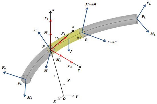
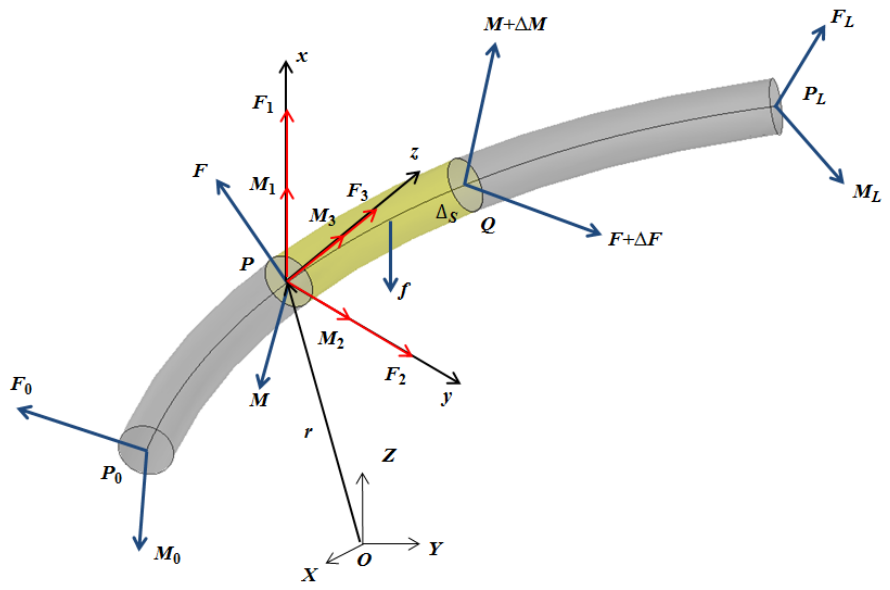
As shown in Figure 1, an elastic rod of length L is located in the inertial coordinate system O-XYZ; the two ends of this rod are marked as $P_0$ and $P_L$, respectively. The principal vector ${\mathit{F}}_0$ and principal moment ${\mathit{M}}_0$ act on end $P_0$, and the principal vector ${\mathit{F}}_{\mathit{L}}$ and principal moment ${\mathit{M}}_{\mathit{L}}$ act on end $P_L$. The elastic rod is subjected to distributed forces $\mathit{f}$ in addition to the principal vectors and principal moments acting on the ends, and this rod can be regarded as a single-span elastic rod. The arc coordinate s is established from end $P_0$ to end $P_L$ in the centerline of the rod. A cross-section P is intercepted at any point in the arc coordinate s, and the internal force and internal moment on this cross-section are principal vector F and principal moment M. Meanwhile, another cross-section Q is intercepted at an infinitesimal distance ${∆}_s$ from cross-section P, and the internal force and internal moment on this cross-section are principal vector F + $∆$F and principal moment M + $∆$M. The infinitesimal element between cross-section P and cross-section Q is in an equilibrium state, and its equilibrium equation can be written as Equations (1) and (2) [39,40].

$${\displaystyle \frac{\mathrm{d}\mathit{F}}{\mathrm{d}\mathit{s}}}+\mathit{f}=0$$

(1)

$${\displaystyle \frac{\mathrm{d}\mathit{M}}{\mathrm{d}\mathit{s}}}+\mathit{z} \times \mathit{F}=0$$

(2)

where z is the tangential unit vector on cross-section P. The relationship between the vector radius r on the center of cross-section P and the tangent unit vector z can be expressed as Equation (3) [41].

$${\displaystyle \frac{\mathrm{d}\mathit{r}}{\mathrm{d}\mathit{s}}}=\mathit{z}$$

(3)

Figure 1. Equilibrium of infinitesimal element in single-span elastic rod.

By establishing the principal axis coordinate system $P$-xyz at the center of cross-section P, the relationship between the inertial coordinate system O-XYZ and the principal axis coordinate system $P$-xyz can be expressed by the direction cosine matrix composed of Euler angles $\psi$, $\theta$, and $\phi$, as indicated in Equation (4).

$$\left[\begin{array}{c}\mathit{X}\\ \mathit{Y}\\ \mathit{Z}\end{array}\right]=\left[\begin{array}{ccc}\cos \psi \cos \phi -\cos \theta \sin \psi \sin \phi & -\cos \psi \sin \phi -\cos \theta \sin \psi \cos \phi & \sin \theta \sin \psi \\ \sin \psi \cos \phi +\cos \theta \cos \psi \sin \phi & -\sin \psi \sin \phi +\cos \theta \cos \psi \cos \phi & -\sin \theta \cos \psi \\ \sin \theta \sin \phi & \sin \theta \cos \phi & \cos \theta \end{array}\right]\left[\begin{array}{c}\mathit{x}\\ \mathit{y}\\ \mathit{z}\end{array}\right]$$

(4)

The principal vector F can be projected into the principal axis coordinate system using Equation (4), and the components are the axial force $F_3$ along the z-axis and lateral forces $F_1$, $F_2$ along the x-axis and y-axis. Similarly, principal moment M can also be projected into the principal axis coordinate system; the components are torque $M_3$ along the z-axis and bending moments $M_1$, $M_2$ along the x-axis and y-axis. By introducing the curvature-twisting vectors ${\omega }_1$, ${\omega }_2$, and ${\omega }_3$, the equilibrium equation can be rewritten into component equations in the principal axis coordinate system $P$-xyz, as expressed in Equation (5) [42].

$$\begin{array}{c} {\displaystyle \frac{\mathrm{d} F_1}{\mathrm{d} s}}+{\omega }_2{F}_3 – {\omega }_3{F}_2+f_1=0\end{array}$$

(5a)

$${\displaystyle \frac{\mathrm{d} F_2}{\mathrm{d} s}}+{\omega }_3{F}_1 – {\omega }_1{F}_3+f_2=0$$

(5b)

$${\displaystyle \frac{\mathrm{d} F_3}{\mathrm{d} s}}+{\omega }_1{F}_2 –{ \omega }_2{F}_1+{ f}_3=0$$

(5c)

$${\displaystyle \frac{\mathrm{d} M_1}{\mathrm{d} s}}+{ \omega }_2{M}_3 -{ \omega }_3{M}_2 -{ F}_2=0$$

(5d)

$${\displaystyle \frac{\mathrm{d} M_2}{\mathrm{d} s}}+{\omega }_3{M}_1 – {\omega }_1{M}_3+{ F}_1=0$$

(5e)

$${\displaystyle \frac{\mathrm{d} M_3}{\mathrm{d} s}}+{ \omega }_1{M}_2 -{ \omega }_2{M}_1=0$$

(5f)

where $f_1$, $f_2$, and $f_3$ are the components of the distributed forces in the principal axis coordinate system. The curvature-twisting vectors ${\omega }_1$, ${\omega }_2$, and ${\omega }_3$ satisfy the constitutive relations in Equation (6).

$${M_1=A \omega }_1,{M_2=B \omega }_2,{M_3= C \omega }_3$$

(6)

where A and B are the bending rigidities of the cross-section, and the bending rigidities satisfy A = B for a circular cross-section. C is the torsional rigidity of the cross-section. The relationship between the Euler angles and curvature-twisting vectors is provided in Equation (7).

$${\displaystyle \frac{\mathrm{d}\psi }{\mathrm{d}s}}={\displaystyle \frac{\sin \phi }{\sin \theta }}{ \omega }_1+{\displaystyle \frac{\cos \phi }{\sin \theta }}{ \omega }_2$$

(7a)

$${\displaystyle \frac{\mathrm{d}\theta }{\mathrm{d}s}}=\cos \phi { \omega }_1+s\mathrm{in}\phi { \omega }_2$$

(7b)

$${\displaystyle \frac{\mathrm{d}\phi }{\mathrm{d}s}}={ \omega }_3-\left({\displaystyle \frac{\sin \phi { \omega }_1+\cos \phi { \omega }_2}{\sin \theta }}\right) \cos \theta$$

(7c)

The position of any cross-section in the elastic rod can be described by the components of the vector radius X, Y, and Z in the inertial coordinate system O-XYZ. The relationship between the Euler angles and components of the vector radius is given by Equation (8).

$${\displaystyle \frac{\mathrm{d}X}{\mathrm{d}s}}=\sin \theta \sin \psi$$

(8a)

$${\displaystyle \frac{\mathrm{d}Y}{\mathrm{d}s}}=-\sin \theta \cos \psi$$

(8b)

$${\displaystyle \frac{\mathrm{d}Z}{\mathrm{d}s}}=-\cos \theta$$

(8c)

2.2. Constraint Equation and Degree of Freedom

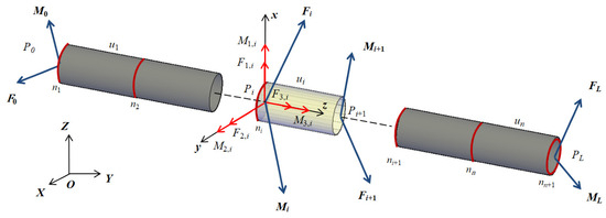
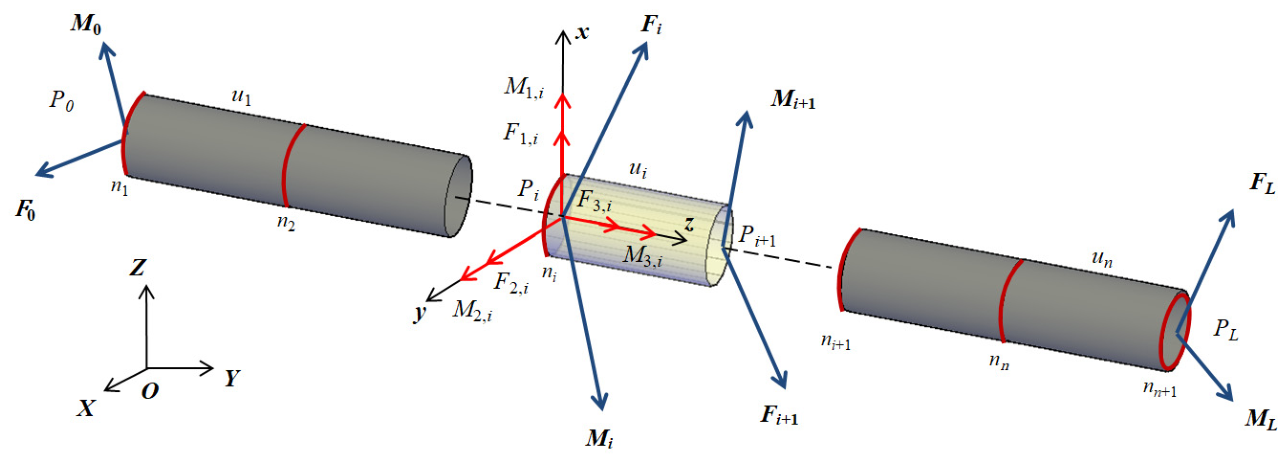
As shown in Figure 2, the single-span elastic rod is discretized into n units and n + 1 nodes, with the length of each unit as $L_i$ [43,44]. Node 1 is located at end $P_0$, and node n + 1 is located at end $P_L$. Taking unit i as an example, this unit is located between node i and node i + 1. The position of the cross-section at node i can be determined by the components of the vector radius in the inertial coordinate system $X_i$, $Y_i$, and $Z_i$. The principal axis coordinate system $P_i$-xyz at node I is established, and the relationship between the coordinate systems O-XYZ and $P_i$-xyz can be expressed by the direction cosine matrix composed of Euler angles ${\psi }_i$, ${\theta }_i$, and ${\phi }_i$. The principal vector can be projected into the principal axis coordinate system, and the components are the axial force $F_{3,i}$ along the z-axis and lateral forces $F_{1,i}$, $F_{2,i}$ along the x-axis and y-axis, respectively. The principal moment can also be projected into the principal axis coordinate system, and the components are torque $M_{3,i}$ along the z-axis and bending moments $M_{1,i}$ and $M_{2,i}$ along the x-axis and y-axis, respectively. Similarly, the principal axis coordinate system $P_{i+1}$-xyz can also be established at node I + 1, and other 12 parameters on the cross-section $P_{i+1}$ are obtained: $X_{i+1}$, $Y_{i+1}$, $Z_{i+1}$, ${\psi }_{i+1}$, ${\theta }_{i+1}$, ${\phi }_{i+1}$, $F_{1,i+1}$, $F_{2,i+1}$, $F_{3,i+1}$, $M_{1,i+1}$, $M_{2,i+1}$, and $M_{3,i+1}$. The equilibrium equation in unit i can be written by the parameters of node i and node i + 1, as expressed in Equation (9).

$$F_{1,i+1}=F_{1,i}+\left[-\left({\displaystyle \frac{{\omega }_{2,i+1}+{\omega }_{2,i}}{2}}\right)\left({\displaystyle \frac{F_{3,i+1}+F_{3,i}}{2}}\right)+\left({\displaystyle \frac{{\omega }_{3,i+1}+{\omega }_{3,i}}{2}}\right)\left({\displaystyle \frac{F_{2,i+1}+F_{2,i}}{2}}\right)+f_{1,i}\right]L_i$$

(9a)

$$F_{2,i+1}=F_{2,i}+\left[-\left({\displaystyle \frac{{\omega }_{3,i+1}+{\omega }_{3,i}}{2}}\right)\left({\displaystyle \frac{F_{1,i+1}+F_{1,i}}{2}}\right)+\left({\displaystyle \frac{{\omega }_{1,i+1}+{\omega }_{1,i}}{2}}\right)\left({\displaystyle \frac{F_{3,i+1}+F_{3,i}}{2}}\right)+f_{2,i}\right]L_i$$

(9b)

$$F_{3,i+1}=F_{3,i}+\left[-\left({\displaystyle \frac{{\omega }_{1,i+1}+{\omega }_{1,i}}{2}}\right)\left({\displaystyle \frac{F_{2,i+1}+F_{2,i}}{2}}\right)+\left({\displaystyle \frac{{\omega }_{2,i+1}+{\omega }_{2,i}}{2}}\right)\left({\displaystyle \frac{F_{1,i+1}+F_{1,i}}{2}}\right)+f_{3,i}\right]L_i$$

(9c)

$$M_{1,i+1}=M_{1,i}+\left[-\left({\displaystyle \frac{{\omega }_{2,i+1}+{\omega }_{2,i}}{2}}\right)\left({\displaystyle \frac{M_{3,i+1}+M_{3,i}}{2}}\right)+\left({\displaystyle \frac{{\omega }_{3,i+1}+{\omega }_{3,i}}{2}}\right)\left({\displaystyle \frac{M_{2,i+1}+M_{2,i}}{2}}\right)+\left({\displaystyle \frac{F_{2,i+1}+F_{2,i}}{2}}\right)\right]L_i$$

(9d)

$$M_{2,i+1}=M_{2,i}+\left[-\left({\displaystyle \frac{{\omega }_{3,i+1}+{\omega }_{3,i}}{2}}\right)\left({\displaystyle \frac{M_{1,i+1}+M_{1,i}}{2}}\right)+\left({\displaystyle \frac{{\omega }_{1,i+1}+{\omega }_{1,i}}{2}}\right)\left({\displaystyle \frac{M_{3,i+1}+M_{3,i}}{2}}\right)+\left({\displaystyle \frac{F_{1,i+1}+F_{1,i}}{2}}\right)\right]L_i$$

(9e)

$$M_{3,i+1}=M_{3,i}+\left[-\left({\displaystyle \frac{{\omega }_{1,i+1}+{\omega }_{1,i}}{2}}\right)\left({\displaystyle \frac{M_{2,i+1}+M_{2,i}}{2}}\right)+\left({\displaystyle \frac{{\omega }_{2,i+1}+{\omega }_{2,i}}{2}}\right)\left({\displaystyle \frac{M_{1,i+1}+M_{1,i}}{2}}\right)\right]L_i$$

(9f)

where $f_{1,i}$, $f_{2,i}$, and $f_{3,i}$ are the distributed forces in unit i. ${\omega }_{1,i}$, ${\omega }_{2,i}$, ${\omega }_{3,i}$, ${\omega }_{1,i+1}$, ${\omega }_{2,i+1}$, and ${\omega }_{3,i+1}$ are the curvature-twisting vectors at node i and node i + 1, respectively. Meanwhile, Equations (7) and (8) can also be rewritten by the parameters of node i and node i + 1, as shown in Equation (10).

$${\psi }_{i+1}={\psi }_i+[\sin \left({\displaystyle \frac{{\phi }_{i+1}+{\phi }_i}{2}}\right)\left({\displaystyle \frac{{\omega }_{1,i+1}+{\omega }_{1,i}}{2}}\right)+\cos \left({\displaystyle \frac{{\phi }_{i+1}+{\phi }_i}{2}}\right)\left({\displaystyle \frac{{\omega }_{2,i+1}+{\omega }_{2,i}}{2}}\right)]{\displaystyle \frac{L_i}{\sin \left(\frac{{\theta }_{i+1}+{\theta }_i}{2}\right)}}$$

(10a)

$${\theta }_{i+1}={\theta }_i+\left[\cos \left({\displaystyle \frac{{\phi }_{i+1}+{\phi }_i}{2}}\right)\left({\displaystyle \frac{{\omega }_{1,i+1}+{\omega }_{1,i}}{2}}\right)-\sin \left({\displaystyle \frac{{\phi }_{i+1}+{\phi }_i}{2}}\right)\left({\displaystyle \frac{{\omega }_{2,i+1}+{\omega }_{2,i}}{2}}\right)\right]L_i$$

(10b)

$${\phi }_{i+1}={\phi }_i+\left[\left({\displaystyle \frac{{\omega }_{3,i+1}+{\omega }_{3,i}}{2}}\right)-\left(\sin \left({\displaystyle \frac{{\phi }_{i+1}+{\phi }_i}{2}}\right)\left({\displaystyle \frac{{\omega }_{1,i+1}+{\omega }_{1,i}}{2}}\right)+\cos \left({\displaystyle \frac{{\phi }_{i+1}+{\phi }_i}{2}}\right)\left({\displaystyle \frac{{\omega }_{2,i+1}+{\omega }_{2,i}}{2}}\right)\right)\cot {\displaystyle \frac{{\theta }_{i+1}+{\theta }_i}{2}}\right]L_i$$

(10c)

$$X_{i+1}=X_i+\left[\sin \left({\displaystyle \frac{{\theta }_{i+1}+{\theta }_1}{2}}\right)\sin \left({\displaystyle \frac{{\psi }_{i+1}+{\psi }_i}{2}}\right)\right]L_i$$

(10d)

$$Y_{i+1}=Y_i-[\sin \left({\displaystyle \frac{{\theta }_{i+1}+{\theta }_i}{2}}\right)\cos \left({\displaystyle \frac{{\psi }_{i+1}+{\psi }_i}{2}}\right)]L_i$$

(10e)

$$Z_{i+1}=Z_i-\cos \left({\displaystyle \frac{{\theta }_{i+1}+{\theta }_i}{2}}\right)L_i$$

(10f)

Figure 2. Discrete element in single-span elastic rod.

Equations (9) and (10) are the constraint equations of unit i. Thus, there are 12n constraint equations and 12(n + 1) node parameters for the discrete system of the elastic rod with n units. The number of independent parameters can be limited to 12 by the 12n constraint equations after all units are connected. Thus, the discrete system can be closed when any 12 of the node parameters are known, and then the other node parameters can be obtained by the constraint equations. However, the known node parameters only appear at node 1 and node n + 1 for a single-span elastic rod. Therefore, the deformation, attitude, and position of the rod are determined only when 12 of the 24 parameters on the two ends are given. According to the above analysis, the degree of freedom in the single-span elastic rod is 12.

These 12 degrees of freedom directly determine the strategy for selecting boundary conditions in the subsequent calculation, since only 12 parameters can be independently prescribed at the two ends, they must be chosen from the 24 parameters according to the criteria of mutual correspondence, exclusion, coordination, and necessity (see Section 2.3). This conclusion provides the theoretical basis for the classification of boundary conditions in Table 1 and ensures the closure of the equation system in the discrete solution procedure.

Table 1. Types of boundary conditions under the necessity criterion.

Type	Number of Prescribed Displacements at P0 (i)	Combinations at P0	Range of j at PL	Combinations at PL for Given j	Total
1	0	$\left(\begin{array}{c}6\\ 0\end{array}\right)=1$	j = 6	$\left(\begin{array}{c}0\\ 6-6\end{array}\right)=1$	1
2	1	$\left(\begin{array}{c}6\\ 1\end{array}\right)=6$	j = 5, 6	${\displaystyle {\sum }_{j=5}^6\left(\begin{array}{c}1\\ j-5\end{array}\right)}=2$	12
3	2	$\left(\begin{array}{c}6\\ 2\end{array}\right)=15$	j = 4, 5, 6	${\displaystyle {\sum }_{j=4}^6\left(\begin{array}{c}2\\ j-4\end{array}\right)}=4$	60
4	3	$\left(\begin{array}{c}6\\ 3\end{array}\right)=20$	j = 3, 4, 5, 6	${\displaystyle {\sum }_{j=3}^6\left(\begin{array}{c}3\\ j-3\end{array}\right)}=8$	160
5	4	$\left(\begin{array}{c}6\\ 4\end{array}\right)=15$	j = 2, 3, 4, 5, 6	${\displaystyle {\sum }_{j=2}^6\left(\begin{array}{c}4\\ j-2\end{array}\right)}=16$	240
6	5	$\left(\begin{array}{c}6\\ 5\end{array}\right)=6$	j = 1, …, 6	${\displaystyle {\sum }_{j=1}^6\left(\begin{array}{c}5\\ j-1\end{array}\right)}=32$	192
7	6	$\left(\begin{array}{c}6\\ 6\end{array}\right)=1$	j = 0, …, 6	${\displaystyle {\sum }_{j=0}^6\left(\begin{array}{c}6\\ j\end{array}\right)}=64$	64
Total					729

2.3. Boundary Condition

2.3.1. Criterion of Boundary Condition

It can be concluded from Section 2.2 that there are 24 parameters on the two ends of a single-span elastic rod, which are called the boundary parameters. Generally, the deformation, attitude, and position of the elastic rod can be determined when 12 boundary parameters are given [45,46]. However, the boundary condition is not an arbitrary combination of boundary parameters, and the selection of these parameters should meet specific criteria. To better explain these criteria, we now introduce four basic concepts related to the boundary condition, which are as follows.

(1)

Generalized displacement: Angular displacements and linear displacements in the boundary condition, which can be used to control the attitude and position of the elastic rod’s end, respectively. The generalized displacement could be a single parameter of the Euler angle or coordinate, and an equation composed of these parameters. However, only six independent generalized displacements exist on one end of the elastic rod, and their expressions can only be established in the inertial coordinate system.

(2)

Generalized force: Moments and forces in the boundary condition. The generalized force could be a component of the principal moment or principal force in the inertial coordinate system, and an equation of these components with generalized displacements. However, only six independent generalized forces exist on one end of the elastic rod, and their expressions vary in different coordinate systems.

(3)

Mutual correspondence: The relationship of one-to-one correspondence between the generalized force and the generalized displacement in a certain direction. For example, the principal vector component corresponds to the linear displacement in the same direction, and the principal moment component corresponds to the angular displacement in the same direction.

(4)

Mutual exclusion: The generalized force and generalized displacement cannot be simultaneously given when they have a relationship of mutual correspondence.

Based on the theoretical analysis, the boundary condition should meet these criteria that can entirely determine the deformation, attitude, and position of the single-span elastic rod, which are as follows.

(1)

Mutual correspondence and exclusion: At the end of the elastic rod, the generalized force and generalized displacement in the same direction have the property of mutual correspondence and mutual exclusion.

(2)

Coordination: The given generalized forces on the ends of the elastic rod need to meet the mechanical equilibrium equation.

(3)

Necessity: For each of the six directions (three translations and three rotations), at least one end must have a prescribed displacement. This prevents the physically inadmissible case where a direction has no displacement prescribed at either end, which would leave a rigid-body mode unconstrained.

Undoubtedly, the necessity in boundary condition criteria does not need to be met when the elastic rod’s rotations or coordinates are not entirely determined. For example, a flexible shaft with uniform rotation can be simulated as long as 5 generalized displacements are given on two ends.

2.3.2. Mutual Correspondence of Boundary Parameters

Taking end $P_0$ as an example, the criterion of mutual correspondence and exclusion between the generalized displacements and the generalized forces for the single-span elastic rod is illustrated. There is a principal axis coordinate system $P_0$-xyz established at end $P_0$, and the direction cosine matrix between coordinate system O-XYZ and coordinate system $P_0$-xyz can be expressed by the Euler angles ${\psi }_0$, ${\theta }_0$, and ${\phi }_0$, as shown in Equation (11).

$$\begin{gathered} \mathit{A}(m,n)=\left[\begin{array}{ccc}\cos {\psi }_0 \cos {\phi }_0-\cos {\theta }_0\sin {\psi }_0\sin {\phi }_0& -\cos {\psi }_0 \sin {\phi }_0-\cos {\theta }_0\sin {\psi }_0\cos {\phi }_0& \sin {\theta }_0\sin {\psi }_0\\ \sin {\psi }_0 \cos {\phi }_0+\cos {\theta }_0\cos {\psi }_0\sin {\phi }_0& -\sin {\psi }_0 \sin {\phi }_0+\cos {\theta }_0\cos {\psi }_0\cos {\phi }_0& -\sin {\theta }_0\cos {\psi }_0\\ \sin {\theta }_0\sin {\phi }_0& \sin {\theta }_0\cos {\phi }_0& \cos {\theta }_0\end{array}\right] \\ (m=1,2,3;n=1,2,3) \end{gathered}$$

(11)

Then, the relationship of the two coordinate systems can be expressed as Equation (12).

$$\left[\begin{array}{c}\mathit{X}\\ \mathit{Y}\\ \mathit{Z}\end{array}\right]=\mathit{A}\left[\begin{array}{c}\mathit{x}\\ \mathit{y}\\ \mathit{z}\end{array}\right]$$

(12)

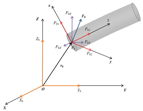
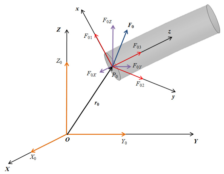
As shown in Figure 3, there are many boundary parameters at end $P_0$. Among them, $F_{01}$, $F_{02}$, and $F_{03}$ are the components of the principal vector ${\mathit{F}}_{\mathbf{0}}$ in the principal axis coordinate system. $X_0$, $Y_0$, and $Z_0$ are the components of vector radius ${\mathit{r}}_{\mathbf{0}}$, which can control the position of end $P_0$.

Figure 3. Relationship of mutual correspondence between principal vector components and vector radius components.

The principal vector ${\mathit{F}}_{\mathbf{0}}$ can also be projected into the inertial coordinate system O-XYZ, and the components of the principal vector are marked as $F_{0X}$, $F_{0Y}$, and $F_{0Z}$, respectively. $F_{0X}$, $F_{0Y}$, and $F_{0Z}$ can be converted by $F_{01}$, $F_{02}$, and $F_{03}$ through the direction cosine matrix, as indicated in Equation (13).

$$\left[\begin{array}{c}{F}_{0X}\\ F_{0Y}\\ F_{0Z}\end{array}\right]=\mathit{A}\left[\begin{array}{c}{F}_{01}\\ F_{02}\\ F_{03}\end{array}\right]$$

(13)

Obviously, the components of the principal vector $F_{0X}$, $F_{0Y}$, and $F_{0Z}$ are generalized forces, which have the criterion of mutual correspondence and exclusion with generalized displacements $X_0$, $Y_0$, and $Z_0$, respectively. Moreover, the three relational expressions of $F_{0X}$, $F_{0Y}$, and $F_{0Z}$ (Equation (13)) can be regarded as generalized forces, and the expressions also have the criterion of mutual correspondence and exclusion with $X_0$, $Y_0$, and $Z_0$, respectively.

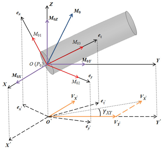
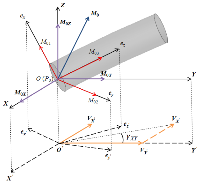
As shown in Figure 4, when moving the center of end $P_0$ to the origin of the inertial coordinate system O-XYZ, $M_{01}$, $M_{02}$, and $M_{03}$ are the components of the principal moment $M_0$ in the principal axis coordinate system $P_0$-xyz. Similarly, the principal moment $M_0$ can also be projected into the inertial coordinate system O-XYZ, and the components are marked as $M_{0X}$, $M_{0Y}$, and $M_{0Z}$, respectively. $M_{0X}$, $M_{0Y}$, and $M_{0Z}$ can be converted by $M_{01}$, $M_{02}$, and $M_{03}$ through the direction cosine matrix, as indicated in Equation (14).

$$\left[\begin{array}{c}{M}_{0X}\\ M_{0Y}\\ M_{0Z}\end{array}\right]=\mathit{A}\left[\begin{array}{c}{M}_{01}\\ M_{02}\\ M_{03}\end{array}\right]$$

(14)

Figure 4. Relationship of mutual correspondence between principal moment components and attitude angles of end.

Although Euler angles ${\psi }_0$, ${\theta }_0$, and ${\phi }_0$ can control the attitude of end $P_0$, they cannot directly correspond to generalized forces $M_{01}$, $M_{02}$, $M_{03}$ or $M_{0X}$, $M_{0Y}$, $M_{0Z}$. To explain how these parameters satisfy the mutual correspondence and exclusion, finding the generalized displacements corresponding to the principal vector moment components is the first step.

The plane determined by the X-axis and Y-axis of the inertial coordinate system is defined as plane XY, and the vertical projection plane $X^{\prime }{Y}^{\prime }$ passing through point $O^{\prime }$ is established to illustrate the relationships of different projections on plane XY. The basic vectors of the principal axis coordinate system ${\mathit{e}}_{\mathit{x}}$, ${\mathit{e}}_{\mathit{y}}$, ${\mathit{e}}_{\mathit{z}}$ can be projected onto a plane $X^{\prime }{Y}^{\prime }$ and marked as ${\mathit{e}}_{{\mathit{x}}^{\prime }}$, ${\mathit{e}}_{{\mathit{y}}^{\prime }}$, and ${\mathit{e}}_{{\mathit{z}}^{\prime }}$, respectively. ${\mathit{e}}_{{\mathit{x}}^{\prime }}$, ${\mathit{e}}_{{\mathit{y}}^{\prime }}$, and ${\mathit{e}}_{{\mathit{z}}^{\prime }}$ can be expressed as Equation (15).

$$\begin{array}{c}{\mathit{e}}_{{\mathit{x}}^{\prime }}=A\left(1,1\right){\mathit{e}}_{{\mathit{X}}^{\prime }}+A\left(2,1\right){\mathit{e}}_{{\mathit{Y}}^{\prime }}\\ {\mathit{e}}_{{\mathit{y}}^{\prime }}=A\left(1,2\right){\mathit{e}}_{{\mathit{X}}^{\prime }}+A\left(2,2\right){\mathit{e}}_{{\mathit{Y}}^{\prime }}\\ {\mathit{e}}_{{\mathit{z}}^{\prime }}=A\left(1,3\right){\mathit{e}}_{{\mathit{X}}^{\prime }}+A\left(2,3\right){\mathit{e}}_{{\mathit{Y}}^{\prime }}\end{array}$$

(15)

where A(m, n) is the value of row m and column n in Equation (11). ${\mathit{e}}_{{\mathit{X}}^{\prime }}$, ${\mathit{e}}_{{\mathit{Y}}^{\prime }}$ are the basic vectors of the $X^{\prime }$-axis and $Y^{\prime }$-axis. The projections ${\mathit{e}}_{{\mathit{x}}^{\prime }}$, ${\mathit{e}}_{{\mathit{y}}^{\prime }}$, and ${\mathit{e}}_{{\mathit{z}}^{\prime }}$ can be composited in the $X^{\prime }$-axis and $Y^{\prime }$-axis, and the composite vectors ${\mathit{V}}_{{\mathit{X}}^{\prime }}$, ${\mathit{V}}_{{\mathit{Y}}^{\prime }}$ can be expressed as Equation (16).

$$\begin{array}{c}{\mathit{V}}_{{\mathit{X}}^{\prime }}=\left[A\left(1,1\right)+A\left(1,2\right)+A\left(1,3\right)\right]{\mathit{e}}_{{\mathit{X}}^{\prime }}\\ {\mathit{V}}_{{\mathit{Y}}^{\prime }}=\left[A\left(2,1\right)+A\left(2,2\right)+A\left(2,3\right)\right]{\mathit{e}}_{{\mathit{Y}}^{\prime }}\end{array}$$

(16)

By introducing the attitude angle ${\gamma }_{\mathit{XY}}$, the expression of this angle is indicated in Equation (17).

$${\gamma }_{\mathit{XY}}=\mathrm{asin}{\displaystyle \frac{V_{X^{\prime }}}{\sqrt{{\left(V_{X^{\prime }}\right)}^2+{\left(V_{Y^{\prime }}\right)}^2}}}$$

(17)

The attitude angle ${\gamma }_{\mathit{XY}}$ can be regarded as the angular displacement along the $Z^{\prime }$-axis caused by the component of the principal moment $M_{0Z}$. Thus, the attitude angle ${\gamma }_{\mathit{XY}}$ is the generalized displacement corresponding to the generalized force $M_{0Z}$. Similarly, the attitude angles ${\gamma }_{\mathit{YZ}}$ and ${\gamma }_{\mathit{ZX}}$ can also be obtained on plane YZ and plane ZX. The components of the principal moment $M_{0X}$, $M_{0Y}$, and $M_{0Z}$ or the expressions of $M_{0X}$, $M_{0Y}$, and $M_{0Z}$ are regarded as generalized forces, which correspond to the attitude angles ${\gamma }_{\mathit{YZ}}$, ${\gamma }_{\mathit{ZX}}$, and ${\gamma }_{\mathit{XY}}$, respectively.

2.3.3. Types of Boundary Conditions Under Necessity Criterion

According to the necessity criterion of boundary conditions in Section 2.3.1, there must be at least six generalized displacements on the two ends, which need to determine the rotations and coordinates in different directions. This means that the six necessary generalized displacements could not only be located at end $P_0$ or end $P_L$, but also could be dispersed on both ends of the elastic rod. After the necessary generalized displacements are determined, the remaining in the boundary condition can be either generalized forces or generalized displacements. The types of boundary conditions for this type of single-span elastic rod are summarized in Table 1. Here, i and j denote the numbers of directions (out of the six: three translations and three rotations) in which displacement (linear or angular) is prescribed at end P₀ and end P_L, respectively. The necessity criterion requires that for each of the six directions, at least one end has a prescribed displacement; i.e., the state (0, 0) (both ends prescribed forces) is forbidden. Consequently, each direction has three possible states: displacement only at P₀, displacement only at P_L, or displacement at both ends. Thus, the total number of valid boundary condition combinations is 3⁶ = 729. The table classifies these combinations by i and verifies the total.

The classification covers all boundary conditions that satisfy the necessity criterion (at least one end with prescribed displacement in each direction), thereby ensuring a well-posed mechanical model with a unique solution. Moreover, all end-constraint types encountered in practical applications (e.g., fixed end, free end, hinged end) can be categorized into the above scheme without omitting any valid combination.

3. Solution of the Mechanical Model

In addition to Euler angles $\psi$, $\theta$, and $\phi$, Euler quaternions $q_1$, $q_2$, $q_3$, and $q_4$ can also be used as the conversion parameters between the inertial coordinate system O-XYZ and the principal axis coordinate system $P$-xyz, and these parameters can be converted to each other [47]. However, using Euler angles will not only lead to singularity, but also reduce the computational efficiency because the equations have trigonometric functions. In contrast, using quaternions can effectively avoid the above problems. Thus, in this work, both approaches replace Euler angles with Euler quaternions, and the derivation procedure of the single-span elastic rod equilibrium equations described by Euler quaternions is illustrated in Appendix A.

Similar to Section 2.2, the single-span elastic rod is discretized into n units and n + 1 nodes. Taking unit i as an example, this unit is located between node i and node i + 1. Node i has the parameters of Euler quaternions $q_{1,i}$, $q_{2,i}$, $q_{3,i}$, $q_{4,i}$, derivatives of quaternions $Q_{1,i}$, $Q_{2,i}$, $Q_{3,i}$, $Q_{4,i}$, components of the principal vector $F_{1,i}$, $F_{2,i}$, $F_{3,i}$, and components of vector radius $X_i$, $Y_i$, $Z_i$. There are only 12 independent parameters at node i because the number of independent quaternions and their derivatives is 3. Similarly, node i + 1 also has the parameters $q_{1,i+1}$, $q_{2,i+1}$, $q_{3,i+1}$, $q_{4,i+1}$, $Q_{1,i+1}$, $Q_{2,i+1}$, $Q_{3,i+1}$, $Q_{4,i+1}$, $F_{1,i+1}$, $F_{2,i+1}$, $F_{3,i+1}$, $X_{i+1}$, $Y_{i+1}$, and $Z_{i+1}$. According to the derivation of Equation (A11), the single-span elastic rod’s constraint equations described by Euler quaternions can be rewritten as Equation (18).

$$\begin{gathered} H_{m, i}(q_{1,i},q_{1,i+1}, q_{2,i},q_{2,i+1}, q_{3,i}, q_{3,i+1}, q_{4,i},q_{4,i+1}, \\ {Q}_{1,i},Q_{1,i+1},Q_{2,i},Q_{2,i+1},Q_{3,i},Q_{3,i+1},Q_{4,i},Q_{4,i+1}, \\ {F}_{1,i},{ F}_{1,i+1},{ F}_{2,i},{ F}_{2,i+1}, F_{3,i}, F_{3,i+1})=0 (m =1,2,\dots ,11; I =1,2,3,\dots ,n) \end{gathered}$$

(18)

Equation (18) is a discretized differential equation with 11n equations and 11(n + 1) node parameters. To make the equations closed, 11 additional generalized displacements and generalized forces have to be found at end $P_0$ and end $P_L$.

It should be noted that Equation (18) involves only the mechanical variables (quaternions, their derivatives, and forces) and does not include the nodal coordinates. The system of Equation (18) has 11n equations and 11(n + 1) nodal parameters, but after applying the quaternion normalization constraints (Equation (A2)) and their derivative relations (Equation (A3)), the number of independent parameters per node reduces to nine. With only these nine independent parameters, the spatial position of the single-span elastic rod cannot be uniquely determined because the rod can undergo rigid-body translations without changing its internal forces and moments. To fully define the rod’s configuration, the coordinates of at least one end must be specified. These three geometric conditions, together with the 9 independent mechanical parameters, yield a total of 12 independent parameters per node, consistent with the 12 degrees of freedom derived in Section 2. Therefore, in addition to the 11 boundary conditions already mentioned, the three coordinates of one end are prescribed separately, resulting in a total of 12 boundary conditions.

Taking end $P_0$ as an example, the attitude of this end can be controlled by the direction cosine, which is composed of Euler quaternions $q_{01}$, $q_{02}$, $q_{03}$, and $q_{04}$, as expressed in Equation (A1). Although the conversion parameters have changed from ${\psi }_0$, ${\theta }_0$, ${\phi }_0$ to $q_{01}$, $q_{02}$, $q_{03}$, $q_{04}$, the direction cosine matrix between the principal axis coordinate system $P_0$-xyz and the inertial coordinate system O-XYZ does not change.

The components of the principal moment $M_{01}$, $M_{02}$, and $M_{03}$ can be converted into the expressions of quaternions’ derivatives $Q_{01}$, $Q_{02}$, $Q_{03}$, and $Q_{04}$ through Equations (6) and (A3), as expressed in Equation (19).

$$\begin{array}{c}{Q}_{01}={\displaystyle \frac{1}{2}}(-q_{1,2}{\omega }_{01} – q_{1,3}{\omega }_{02} – q_{1,4}{\omega }_{03})\\ Q_{02}={\displaystyle \frac{1}{2}} (q_{1,1}{\omega }_{01}-q_{1,4}{\omega }_{02}+q_{1,3}{\omega }_{03})\\ \begin{array}{c}{Q}_{03}={\displaystyle \frac{1}{2}} (q_{1,4}{\omega }_{01}+q_{1,1}{\omega }_{02 }– q_{1,2}{\omega }_{03})\\ Q_{04}={\displaystyle \frac{1}{2}}(-q_{1,3}{\omega }_{01}+q_{1,2}{\omega }_{02}+q_{1,1}{\omega }_{03})\end{array}\end{array}$$

(19)

where ${\omega }_{01}$, ${\omega }_{02}$, and ${\omega }_{03}$ are curvature-twisting vectors. $Q_{1,1}$, $q_{1,2}$, $q_{1,3}$, and $q_{1,4}$ are undetermined Euler quaternions at node 1. Equation (19) can be regarded as generalized forces when $M_{01}$, $M_{02}$, and $M_{03}$ are all given.

Moving the center of end $P_0$ to a certain position in the inertial coordinate system O-XYZ, the expressions of coordinates $X_L$, $Y_L$, and $Z_L$ can be regarded as the generalized displacements on end $P_L$, as indicated in Equation (A15). The elastic rod system is closed by adding 11 constraint equations of the boundary condition to Equation (18). Finally, the attitude, position, and deformation of the elastic rod can be calculated through a programming calculation [48].

4. Verification of the Mechanical Model

The end constraints of single-span elastic rods with known mathematical curve deformations are taken as boundary conditions, and the elastic rod deformations are calculated using the discrete method introduced in Section 3. Then, the rationality of this method is verified by comparing the elastic rods with their corresponding mathematical curves.

4.1. Circular Elastic Rod

A single-span elastic rod is located in the inertial coordinate system O-XYZ and becomes a two-dimensional circular rod under particular boundary conditions. The radius and length of this elastic rod are R and L, respectively. The center of end $P_0$ is fixed at point O, and the direction of the principal axis coordinate system $P_0$xyz is established on end $P_0$, where the z-axis and x-axis are consistent with the Y-axis and X-axis, respectively. Meanwhile, the attitude and position of end $P_L$ are variable with the change in bending moment along the x-axis, $M_{L1}$. In addition, no distributed force exists on the elastic rod. The boundary condition can be rewritten into constraint equations based on the above analysis, as indicated in Equation (20).

$$H_{1,n+1}=q_{1,1}-{ q}_{01}$$

(20a)

$$H_{2,n+1}=q_{2,1}-{ q}_{02}$$

(20b)

$$H_{3,n+1}=q_{3,1}-{ q}_{03}$$

(20c)

$$H_{4,n+1}=q_{4,1}-{ q}_{04}$$

(20d)

$$H_{5,n+1}={\displaystyle \frac{1}{2}}\left(-{ q}_{2,n+1}{\omega }_{L1}-{ q}_{3,n+1} {\omega }_{L2}-{ q}_{4,n+1}{\omega }_{L3}\right)-{ Q}_{1,n+1}$$

(20e)

$$H_{6,n+1}={\displaystyle \frac{1}{2}}\left(q_{1,n+1}{\omega }_{L1} –{ q}_{4,n+1} {\omega }_{L2}+q_{3,n+1}{\omega }_{L3}\right) –{ Q}_{2,n+1}$$

(20f)

$$H_{7,n+1}= {\displaystyle \frac{1}{2}}\left(q_{4,n+1}{\omega }_{L1}+q_{1,n+1} {\omega }_{L2}-{ q}_{2,n+1}{\omega }_{L3}\right) –{ Q}_{3,n+1}$$

(20g)

$$H_{8,n+1 }={\displaystyle \frac{1}{2}}\left(q_{3,n+1}{\omega }_{L1 }+{ q}_{2,n+1}{\omega }_{L2}+q_{1,n+1}{\omega }_{L3}\right) –{ Q}_{4,n+1}$$

(20h)

$$H_{9,n+1}={ F}_{1,n+1} –{ F}_{L1}$$

(20i)

$$H_{10,n+1}={ F}_{2,n+1}-F_{L2}$$

(20j)

$$H_{11,n+1} =F_{3,n+1}-{ F}_{L3}$$

(20k)

where ${\omega }_{L1}$, ${\omega }_{L2}$, and ${\omega }_{L3}$ are curvature-twisting vectors on end $P_L$. $F_{L1}$, $F_{L2}$, and $F_{L3}$ are components of the principal vector ${\mathit{F}}_{\mathit{L}}$ on end $P_L$. The closed equations for the circular elastic rod are established by combining Equations (18) and (20), and the required parameters in this example are listed in Table 2.

Table 2. Calculation parameters of circular elastic rod.

Parameters	Symbol	Value	Units
Euler quaternions on end $P_0$	${ q}_{01}$	−0.7071	-
	${ q}_{02}$	0.7071	-
	${ q}_{03}$	0.00	-
	${ q}_{04}$	0.00	-
	${ X}_0$	0.00	m
Coordinates of end $P_0$	${ Y}_0$	0.00	m
	${ Z}_0$	0.00	m
Components of principal moment on end $P_0$	$M_{L2}$	0.00	N$·$m
	$M_{L3}$	0.00	N$·$m
Components of principal vector on end $P_0$	${ F}_{L1}$, $F_{L2}$, $F_{L3}$	0.00	N
Length	L	40.00	m
Outer diameter	${ r}_o$	0.05	m
Inner diameter	${ r}_i$	0.02	m
Elastic modulus	E	2.14 · 10−8	Pa
Poisson ratio	$\mu$	0.25	-
Number of units	n	40.00	-

The equations for the circular elastic rod can be solved when the bending moment $M_{L1}$ is given, and the variations of $M_{L1}$ lead to different deformations, positions, and attitudes of this elastic rod. The radius of these elastic rods can be expressed as Equation (21).

$$R={\displaystyle \frac{A}{M_{L1}}}$$

(21)

where A is the bending rigidity and R is the radius of the elastic rod.

Meanwhile, the parameter equations of the mathematical curve with the same deformation as the circular elastic rod can be expressed as Equation (22).

$$\begin{array}{ccc}X\left(s\right)=0, & Y\left(s\right)=R\cos \left({\displaystyle \frac{L·s}{R}}-{\displaystyle \frac{\pi }{2}}\right), & Z\left(s\right)=-R – R\sin \left({\displaystyle \frac{L·s}{R}}-{\displaystyle \frac{\pi }{2}}\right) \end{array} (0 \le s \le L)$$

(22)

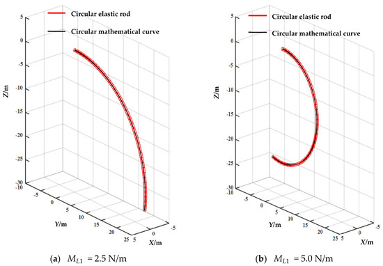
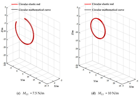
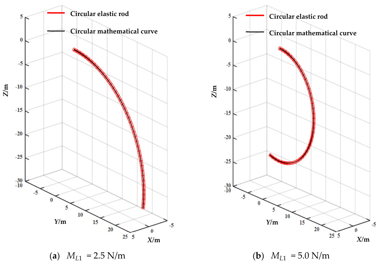
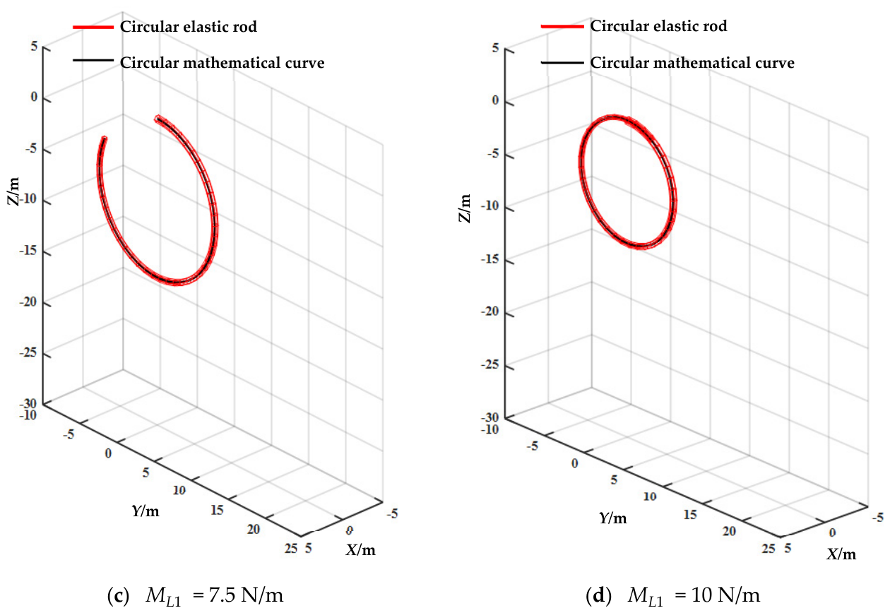
The selections of $M_{L1}$ are 2.5, 5.0, 7.5, and 10.0 N/m, respectively, and then four circular elastic rods are obtained. The deformations of these elastic rods and their corresponding mathematical curves are shown in Figure 5.

Figure 5. Comparison between circular elastic rod and circular mathematical curve.

Comparing the deformations of the circular elastic rods with their corresponding circular mathematical curves, each figure in Figure 5 shows that the centerline of the circular elastic rod entirely coincides with the circular mathematical curve. Taking the bending moment $M_{L1}$ = 2.5 N/m as an example, the coordinates of the circular elastic rod and circular mathematical curve are listed in Table 3.

Table 3. Comparison between circular elastic rod and circular mathematical curve.

Distance from End ${\mathit{P}}_0$ (m)	Model	X (m)	Y (m)	Z (m)
10.00	Elastic rod	0.00	9.6971	−2.1096
	Mathematical curve	0.00	9.6965	−2.1109
20.00	Elastic rod	0.00	17.6398	−8.0588
	Mathematical curve	0.00	17.6380	−8.0615
30.00	Elastic rod	0.00	22.3911	−16.7711
	Mathematical curve	0.00	22.3873	−16.7748
40.00	Elastic rod	0.00	23.0911	−26.6700
	Mathematical curve	0.00	23.0848	−26.6738

In Table 3, the coordinate error between the circular elastic rod and the mathematical curve is less than 1 cm, which means that the discrete method of the single-span elastic rod model is basically accurate in the two-dimensional condition.

4.2. Helical Elastic Rod

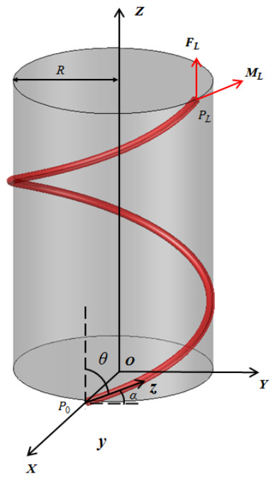
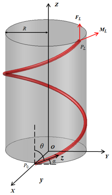
A single-span elastic rod with length L is located in the inertial coordinate system O-XYZ, and it becomes a three-dimensional circular rod under a particular boundary condition, of which the helix diameter R and helix angle $\alpha$ remain unchanged. In addition, no distributed force exists on the elastic rod.

As shown in Figure 6, the center of end $P_0$ is located at coordinates (R, 0, 0) in the inertial coordinate system O-XYZ. The direction of the principal axis coordinate system $P_0$-xyz relative to the inertial coordinate system is determined, and the direction cosine matrix between the two coordinate systems can be expressed as Equation (23).

$$\left[\begin{array}{c}\mathit{X}\\ \mathit{Y}\\ \mathit{Z}\end{array}\right]=\left[\begin{array}{ccc}-1& 0& 0\\ 0& -\cos \theta & \sin \theta \\ 0& \sin \theta & \cos \theta \end{array}\right]\left[\begin{array}{c}\mathit{x}\\ \mathit{y}\\ \mathit{z}\end{array}\right]$$

(23)

where $\theta$ is the nutation angle of the helical elastic rod, which is complementary to the helix angle $\alpha$. The Euler quaternions $q_{01}$, $q_{02}$, $q_{03}$, $q_{04}$ at end $P_0$ can be converted through the conversion relationship between the direction cosine matrix and the quaternions. Principal vector ${\mathit{F}}_{\mathit{L}}$ and principal moment ${\mathit{M}}_{\mathit{L}}$ act on end $P_L$ simultaneously. The components of the principal moment in the principal axis coordinate system $P_L$-xyz should meet special requirements, as indicated in Equation (24).

$$M_{L1}=0,{M_{L2}=B \omega }_0 \sin \theta ,M_{L3}=C {\omega }_{L3}$$

(24)

where ${\omega }_{L3}$ is the curvature-twisting vector along the z-axis. ${\omega }_0$ can be expressed as Equation (25).

$${\omega }_0={\displaystyle \frac{\sin \theta }{R}}$$

(25)

Figure 6. Parameters on helical elastic rod.

The components of the principal moment $M_{L1}$, $M_{L2}$, and $M_{L3}$ can be converted into the expressions of quaternions’ derivatives $Q_{L1}$, $Q_{L2}$, $Q_{L3}$, and $Q_{L4}$ through Equations (6) and (19). In addition, the direction of the principal vector ${\mathit{F}}_{\mathit{L}}$ along the Z-axis is based on the force-spiral theory, and the size of ${\mathit{F}}_{\mathit{L}}$ can be expressed as Equation (26).

$$F_L=C {\omega }_0{\omega }_{L3}-{B{ (\omega }_0)}^2\cos \theta$$

(26)

The principal vector can be projected into the principal axis coordinate system $P_L$-xyz through Equation (A1), as indicated in Equation (27).

$$\begin{gathered} F_{L1}=2\left(q_{2,n+1}{q}_{4,n+1}+{ q}_{1,n+1}{q}_{3,n+1}\right)F_L \\ {F}_{L2}=2\left(q_{3,n+1}{q}_{4,n+1} -{ q}_{1,n+1}{q}_{2,n+1}\right)F_L \\ {F}_{L3}=\left(q_{1,n+1}^2-q_{2,n+1}^2 -{ q}_{3,n+1}^2+q_{4,n+1}^2\right)F_L \end{gathered}$$

(27)

The boundary condition can be rewritten into constraint equations based on the above analysis, as indicated in Equation (28).

$$H_{1,n+1}=q_{1,1}-{ q}_{01}$$

(28a)

$$H_{2,n+1}=q_{2,1}-{ q}_{02}$$

(28b)

$$H_{3,n+1}=q_{3,1}-{ q}_{03}$$

(28c)

$$H_{4,n+1}=q_{4,1}-{ q}_{04}$$

(28d)

$$H_{5,n+1}={\displaystyle \frac{1}{2}}\left(-{ q}_{2,n+1}{\omega }_{L1} -{ q}_{3,n+1} {\omega }_{L2}-{ q}_{4,n+1}{\omega }_{L3}\right)-{ Q}_{1,n+1}$$

(28e)

$$H_{6,n+1}={\displaystyle \frac{1}{2}}\left(q_{1,n+1}{\omega }_{L1} -{ q}_{4,n+1} {\omega }_{L2}+q_{3,n+1}{\omega }_{L3}\right) -{ Q}_{2,n+1}$$

(28f)

$$H_{7,n+1}={\displaystyle \frac{1}{2}}\left(q_{4,n+1}{\omega }_{L1}+q_{1,n+1} {\omega }_{L2}-{ q}_{2,n+1}{\omega }_{L3}\right) -{ Q}_{3,n+1}$$

(28g)

$$H_{8,n+1}={\displaystyle \frac{1}{2}}\left(q_{3,n+1}{\omega }_{L1 }+{ q}_{2,n+1}{\omega }_{L2}+q_{1,n+1}{\omega }_{L3}\right) -{ Q}_{4,n+1}$$

(28h)

$$H_{9,n+1}={ F}_{1,n+1} -{ F}_{L1}$$

(28i)

$$H_{10,n+1}={ F}_{2,n+1}- F_{L2}$$

(28j)

$$H_{11,n+1} =F_{3,n+1}-{ F}_{L3}$$

(28k)

The closed equations for the helical elastic rod are established by combining Equations (18) and (28), and the required parameters in this example are listed in Table 4.

Table 4. Calculation parameters of helical elastic rod.

Parameters	Symbol	Value	Units
Component of principal moment on end $P_0$	$M_{L3}$	0.00	N$·$m
Length	L	40.00	m
Outer diameter	${ r}_o$	0.05	m
Inner diameter	${ r}_i$	0.02	m
Elastic modulus	E	2.14 $·$ 10−8	Pa
Poisson ratio	$\mu$	0.25	-
Number of units	n	40.00	-

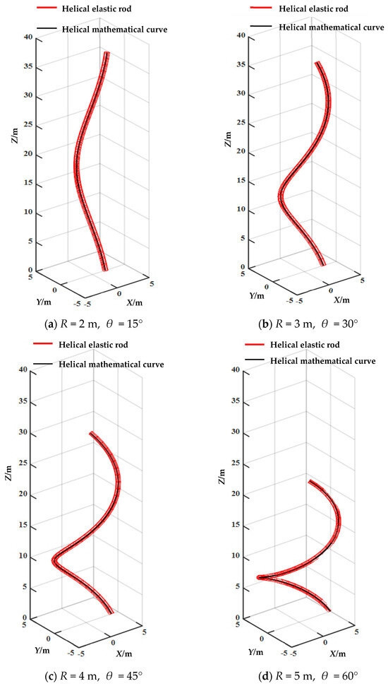
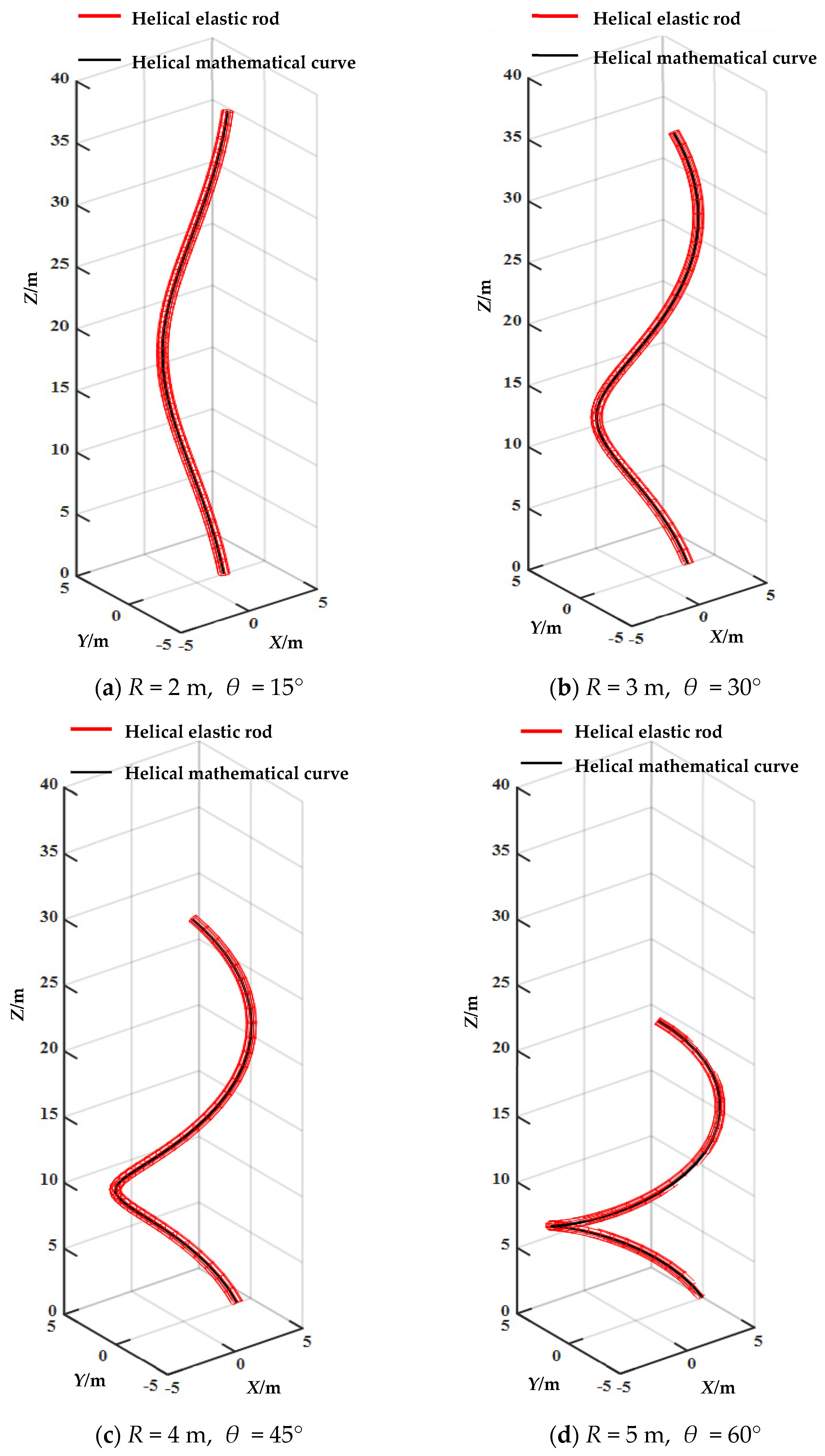
The equations for the helical elastic rod can be solved when the helix diameter R and helix angle $\alpha$ are given, and different combinations of R and $\alpha$ correspond to variable deformations, positions, and attitudes of this rod. Meanwhile, the parameter equations of the mathematical curve in the same deformation as the helical elastic rod can be expressed as Equation (29).

$$\begin{array}{ccc}X\left(s\right)=R\cos \left({s·\omega }_0\right),& Y\left(s\right)=R \sin ({s·\omega }_0),& Z\left(s\right)=s·\cos \theta \end{array} (0 \le s \le L)$$

(29)

The selections of helix diameter R and helix angle $\alpha$ are divided into four types: R = 2 m, $\theta$ = 15°; R = 3 m, $\theta$ = 30°; R = 4 m, $\theta$ = 45°; and R = 5 m, $\theta$= 60°. The deformations of the elastic rods with their corresponding mathematical curves are shown in Figure 7.

Figure 7. Comparison between helical elastic rod and helical mathematical curve.

Comparing the deformations of the helical elastic rods with the helical mathematical curves, each figure in Figure 7 shows that the centerline of the elastic rod entirely coincides with the mathematical curve. Taking the helix diameter R = 5 m and helix angle $\theta$= 60° as an example, the coordinates of the helical elastic rod and helical mathematical curve are listed in Table 5.

Table 5. Comparison between helical elastic rod and helical mathematical curve.

Distance from End ${\mathit{P}}_0$ (m)	Model	X (m)	Y (m)	Z (m)
10.00	Elastic rod	−0.7939	4.9477	5.0192
	Mathematical curve	−0.80278	4.9351	5.0000
20.00	Elastic rod	−4.7570	−1.5554	10.0399
	Mathematical curve	−4.7422	−1.5847	10.0000
30.00	Elastic rod	2.3013	−4.4291	15.0463
	Mathematical curve	2.3256	−4.4263	15.0000
40.00	Elastic rod	3.9281	2.9953	20.0420
	Mathematical curve	3.9954	3.0061	20.0000

In Table 5, the error of coordinates between the helical elastic rod and the helical mathematical curve is less than 7 cm, which means that the discrete method for the single-span elastic rod model is basically accurate. It also shows that the single-span elastic rod model can solve problems involving large deformations in three-dimensional conditions.

4.3. Mesh Convergence Study

A mesh convergence study is performed for both the circular and helical elastic rods using four mesh densities: n = 20, 40, 80, and 160. The Euclidean error, defined as the distance between the computed coordinates and the analytical solution, is evaluated at positions s = 10, 20, 30, and 40 m along the rod. For the circular rod (two-dimensional case), the error is the square root of the sum of squared differences in the Y and Z coordinates; for the helical rod (three-dimensional case), the error additionally includes the X coordinate. The convergence results are presented for the same loading and geometric configurations as in Section 4.1 and Section 4.2. For the circular rod, the bending moment $M_{L1}$ is 2.5 N/m; for the helical rod, the helix diameter R is 5 m and the helix angle θ is 60°.

The errors for the circular rod are listed in Table 6, and those for the helical rod are listed in Table 7. For the circular rod at 40 m, the error decreases from 0.0152 m (n = 20) to 0.0004 m (n = 160); for the helical rod at the same position, the error decreases from 0.2911 m to 0.0127 m. The error decays monotonically with mesh refinement at all sampled positions, and the convergence rate is approximately first-order, consistent with the finite difference scheme employed.

Table 6. Convergence of the circular elastic rod: Euclidean errors at selected positions for different mesh densities.

Distance from End ${\mathit{P}}_0$ (m)	n = 20 Error (m)	n = 40 Error (m)	n = 80 Error (m)	n = 160 Error (m)
10	0.0052	0.0014	0.0005	0.0001
20	0.0106	0.0032	0.0011	0.0003
30	0.0146	0.0053	0.0016	0.0004
40	0.0152	0.0074	0.0020	0.0004

Table 7. Convergence of the helical elastic rod: Euclidean errors at selected positions for different mesh densities.

Distance from End ${\mathit{P}}_0$ (m)	n = 20 Error (m)	n = 40 Error (m)	n = 80 Error (m)	n = 160 Error (m)
10	0.0959	0.0246	0.0064	0.0018
20	0.2014	0.0517	0.0138	0.0043
30	0.2113	0.0524	0.0139	0.0045
40	0.2911	0.0801	0.0245	0.0127

The verification presented in this section is limited to two benchmark cases: a circular curve representing two-dimensional bending under a constant bending moment and a helical curve representing three-dimensional bending and twisting under combined loading. These two cases were selected because they represent fundamental deformation patterns that frequently appear in practical engineering applications, such as planar buckling of drill strings in curved wellbores, helical buckling of cables, landing string subjected to wave loads and current force, sand shape control of flexible manipulators. The good agreement between the numerical results and the analytical solutions, together with the mesh convergence study, demonstrates that the discrete method accurately captures large deformations in both two and three dimensions. While this verification does not exhaust all possible loading or boundary conditions, it provides a rigorous quantitative basis for applying the model to problems exhibiting similar deformation characteristics, including the deep-water landing string analyzed in Section 5. For other specific configurations not covered here, additional validation may be required.

5. Application of the Mechanical Model

Taking the mechanical analysis of a landing string in deep water as an example, the procedures of using the single-span elastic rod model are introduced in detail. The following example of a deep-water landing string serves primarily to illustrate the step-by-step application procedure of the proposed single-span elastic rod model and to demonstrate how selected environmental and operational factors influence the calculated Mises stress. It is not intended as a full-scale engineering analysis but rather as a methodological demonstration. The proposed method can be further extended to more complex problems in deep-water drilling, including the mechanical analysis of risers, landing strings, and drill strings under coupled loads.

5.1. Force Analysis

Deep-water drilling operations before riser deployment include conductor installation, surface wellbore drilling, and cementing. All operations require the use of a landing string. However, the landing string is directly exposed to the sea and has complex deformation and force conditions under the influence of high tensile strength, wave load, current force, heave, and offset of the platform [49]. Therefore, it is necessary to conduct a mechanical analysis of the landing string.

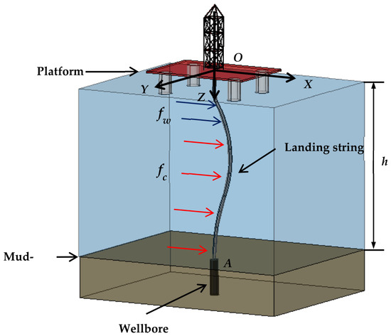
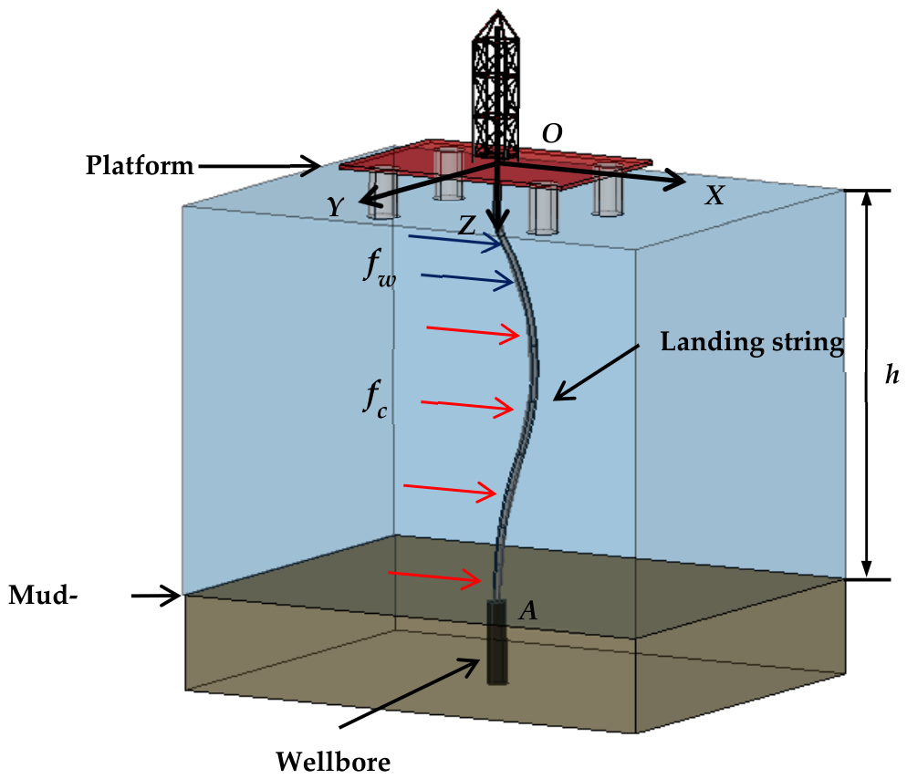
As shown in Figure 8, a landing string is located in the seawater, and the length of the landing string and the depth of seawater are L and h, respectively. The top of the landing string is located in moon pool O and is fixed by wellhead slips. The bottom of the landing string is tripped in the vertical surface wellbore through wellhead A and connected with the preventer, casing, and conductor. There are wave load $f_w$ and current force $f_c$ that exist on the landing string in addition to the buoyed weight. Thus, the landing string can be regarded as a single-span elastic rod.

Figure 8. Force analysis for landing string in deep water.

5.2. Setting of Boundary Condition

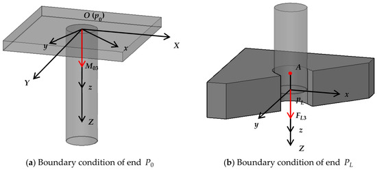
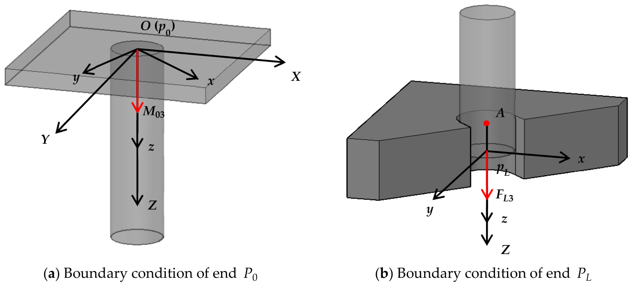
A fixed coordinate system O-XYZ is established at point O, of which the Z-axis is along the vertical direction. As shown in Figure 9a, the top of the landing string is marked as end $P_0$. The principal axis coordinate system $P_0$-xyz is established at end $P_0$, and the direction of the z-axis is consistent with the Z-axis of the fixed coordinate. The component of the principal moment $M_{03}$ can be regarded as a generalized force, which has the criterion of mutual correspondence and exclusion with the angular displacement along the direction of the Z-axis. Therefore, the direction cosine between the Y-axis and the x-axis or y-axis cannot be determined when $M_{03}$ is given. As shown in Figure 9b, the bottom of the landing string is marked as end $P_L$. The principal axis coordinate system $P_L$xyz is established on end $P_L$, of which the z-axis is consistent with the Z-axis of the fixed coordinate system. Then, the direction of the x-axis and y-axis should be determined based on the criterion of necessity. In addition, end $P_L$ can move along the Z-axis as the variable of axial tension $F_{L3}$, which means that the coordinate $Z_L$ cannot be determined when $F_{L3}$ is given.

Figure 9. Boundary condition of landing string.

The boundary condition can be rewritten into constraint equations based on the above analysis, as indicated in Equation (30).

$$H_{1,n+1}=2\left(q_{2,1}{q}_{4,1}+q_{1,1}{q}_{3,1}\right)$$

(30a)

$$H_{2,n+1}=2\left(q_{3,1}{q}_{4,1}-q_{1,1}{q}_{2,1}\right)$$

(30b)

$$H_{3,n+1}=\left(q_{1,1}^2-q_{2,1}^2-q_{3,1}^2+q_{4,1}^2\right)+1$$

(30c)

$$H_{4,n+1}=2\left({-q}_{4,1}{Q}_{1,1}+q_{3,1}{Q}_{2,1}-{ q}_{2,1}{Q}_{3,1}+{ q}_{1,1}{Q}_{4,1}\right)-{\displaystyle \frac{M_{03}}{C}}$$

(30d)

$$H_{5,n+1}=q_{1,n+1}-{ q}_{L1}$$

(30e)

$$H_{6,n+1}=q_{2,n+1}-{ q}_{L2}$$

(30f)

$$H_{7,n+1}=q_{3,n+1}-{ q}_{L3}$$

(30g)

$$H_{8,n+1}=q_{4,n+1}-{ q}_{L4}$$

(30h)

$$H_{9,n+1}={\displaystyle \sum _{i=1}^n}{L}_i{\stackrel{\mathrm{-}}{A}}_i\left(1,3\right)+Y_0-Y_L$$

(30i)

$$H_{10,n+1}={\displaystyle \sum _{i=1}^n}{L}_i{\stackrel{\mathrm{-}}{A}}_i\left(2,3\right)+X_0-{ X}_L$$

(30j)

$$H_{11,n+1}={F_{3,n+1}- F}_{L3}$$

(30k)

where ${ q}_{L1}$, ${ q}_{L2}$, ${ q}_{L3}$, and ${ q}_{L4}$ are Euler quaternions on end $P_L$. ${\stackrel{\mathrm{-}}{\mathit{A}}}_i$(m,n) is the direction cosine matrix at the average position of each unit, and the value corresponding to row m and column n in the matrix can be expressed as Equation (A12). $X_0$, $Y_0$ are the coordinates of end $P_0$. $X_L$, $Y_L$ are the coordinates of end $P_L$.

5.3. Exertion of Distributed Force

The wave load $f_w$ and current force $f_c$ can be regarded as the distributed forces acting on the landing string. The formulas for the wave load and current force are obtained from the Morison equation [48], as indicated in Equations (31) and (32).

$$F_w={\displaystyle \frac{\rho D_o}{2}}{C}_{D}u \left|u\right|+\rho C_m{\displaystyle \frac{\pi D_o^2}{4}}{\displaystyle \frac{\partial u}{\partial t}}$$

(31)

$$f_c={\displaystyle \frac{\rho D_o}{2}}{C}_{D}v \left|v\right|$$

(32)

where $\rho$ is the density of seawater, $D_o$ is the outer diameter of the landing string, $C_D$ is the coefficient of drag force, $C_m$ is the coefficient of inertia force, u is the velocity of the water particle perpendicular to the cylinder, ${\displaystyle \frac{\partial u}{\partial t}}$ is the acceleration of the water particle perpendicular to the cylinder, and v is current velocity. In addition, u and ${\displaystyle \frac{\partial u}{\partial t}}$ can be expressed as Equations (33) and (34), respectively.

$$u ={\displaystyle \frac{\pi H}{T}}{\displaystyle \frac{\cos hk (h-Z)}{\sin h\mathrm{kh}}} \cos \omega t$$

(33)

$${\displaystyle \frac{\partial u}{\partial t}}=-{\displaystyle \frac{2 {\pi }^{2}H}{T^2}}{\displaystyle \frac{\cos hk (h-Z)}{\sin h \mathrm{kh}}}\sin \omega t$$

(34)

$$k={\displaystyle \frac{2\pi }{l}},\omega ={\displaystyle \frac{2\pi }{T}},l={\displaystyle \frac{9.8T^{ 2}}{2\pi }}$$

(35)

where k is the wave number, $\omega$ is circular frequency, H is wave height, T is wave period, h is depth of seawater, Z is calculation depth, l is wave length, and t is time. The current velocity v can be expressed as Equation (36).

$$v={\displaystyle \frac{\left(v_m-v_d\right) Z}{h}}+v_d$$

(36)

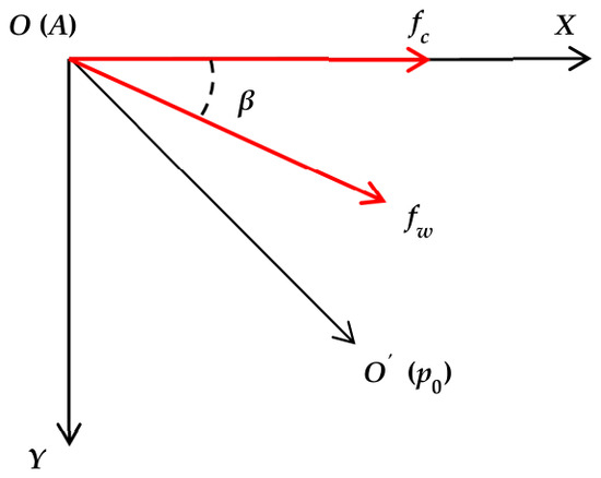
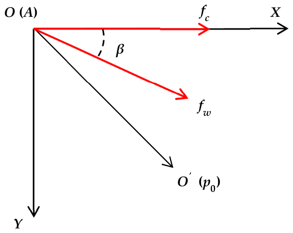
where $v_m$ is the current velocity on the sea surface and $v_d$ is the current velocity on the mudline. By introducing Equation (33) to Equation (35) into Equation (31), and introducing Equation (36) into Equation (32), the wave load and current force varying with the depth of seawater can be obtained. The wave load and current force are regarded as distributed forces acting on the average position of each landing string unit, where the current force direction is consistent with the X-axis. The angle between the wave load and current force is denoted as $\beta$, and the distributed force can be expressed as Equation (37).

$$f_X\left({\stackrel{\mathrm{-}}{Z}}_i\right)=f_w\left({\stackrel{\mathrm{-}}{Z}}_i\right)\sin \beta f_Y \left({\stackrel{\mathrm{-}}{Z}}_i\right)=f_c\left({\stackrel{\mathrm{-}}{Z}}_i\right)+f_w\left({\stackrel{\mathrm{-}}{Z}}_i\right)\cos \beta (i =1,2,3,\dots ,n)$$

(37)

where $f_X\left({\overline{Z}}_i\right)$ and $f_Y\left({\overline{Z}}_i\right)$ are the components of the distributed force along the X-axis and Y-axis, respectively. ${\overline{Z}}_i$ is the average vertical coordinate of each unit. In addition to the current force and wave load, the buoyed weight $G_{Z,i}$ also needs to be considered. Therefore, the distributed force is composed of $f_X\left({\overline{Z}}_i\right)$, $f_Y\left({\overline{Z}}_i\right)$, and $G_{Z,i}$, which can be converted into the principal axis coordinate system $\overline{P_i}$-xyz, as indicated in Equation (38).

$$\begin{array}{c}{\stackrel{\mathrm{-}}{F}}_{1,i}={\stackrel{\mathrm{-}}{\mathit{A}}}_{\mathit{i}}(1,1) f_X\left({\stackrel{\mathrm{-}}{Z}}_i\right)+{\stackrel{\mathrm{-}}{\mathit{A}}}_{\mathit{i}}(2,1) f_Y \left({\stackrel{\mathrm{-}}{Z}}_i\right)+{\stackrel{\mathrm{-}}{\mathit{A}}}_{\mathit{i}}(3,1) G_{Z,I} \\ {\stackrel{\mathrm{-}}{f}}_{2,i}={\stackrel{\mathrm{-}}{\mathit{A}}}_{\mathit{i}}(1,2) f_X\left({\stackrel{\mathrm{-}}{Z}}_i\right)+{\stackrel{\mathrm{-}}{\mathit{A}}}_{\mathit{i}}(2,2) f_Y \left({\stackrel{\mathrm{-}}{Z}}_i\right)+{\stackrel{\mathrm{-}}{\mathit{A}}}_{\mathit{i}}(3,2) G_{Z,i} \\ {\stackrel{\mathrm{-}}{f}}_{3,i}={\stackrel{\mathrm{-}}{\mathit{A}}}_{\mathit{i}}(1,3) f_X\left({\stackrel{\mathrm{-}}{Z}}_i\right)+{\stackrel{\mathrm{-}}{\mathit{A}}}_{\mathit{i}}(2,3) f_Y \left({\stackrel{\mathrm{-}}{Z}}_i\right)+{\stackrel{\mathrm{-}}{\mathit{A}}}_{\mathit{i}}(3,3) G_{Z,i} \end{array}$$

(38)

Equation (38) is introduced into Equation (18), and then the closed equations for the landing string are established by combining Equations (18) and (30).

5.4. Example Calculation

Taking a well as an example, the bottom of the landing string connects the conductor and BHA during the drilling operation. The parameters of the landing string are listed in Table 8.

Table 8. Parameters of landing string.

Parameters	Symbol	Value	Units
Length	L	1300.00	m
Outer diameter	${ D}_o$	0.15	m
Inner diameter	${ D}_i$	0.13	m
Elastic modulus	E	2.14 · 1011	Pa
Poisson ratio	$\mu$	0.34	-
Buoyant weight	$G_Z$	367.30	N/m

According to the statistics for the water around the well in a period of time, the parameters of wave load and current force are listed in Table 9. The parameters in Table 9 are introduced into Equations (33) and (34), and then the variation in wave load on the sea surface can be obtained through Equation (31).

Table 9. Parameters of wave load and current force.

Parameters	Symbol	Value	Units
Density of seawater	$P$	1025.00	kg/${\mathrm{m}}^3$
Coefficient of drag force	$C_D$	1.00	-
Coefficient of inertia force	$C_m$	2.00	-
Wave number	k	0.06	-
Wave height	H	5.10	m
Wave length	l	104.88	m
Wave period	T	8.20	s
Depth of seawater	h	1293.00	m
Current velocity on sea surface	$v_m$	0.75	m/s
Current velocity on mudline	$v_d$	0.05	m/s

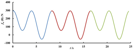
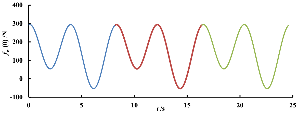
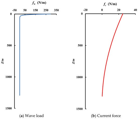
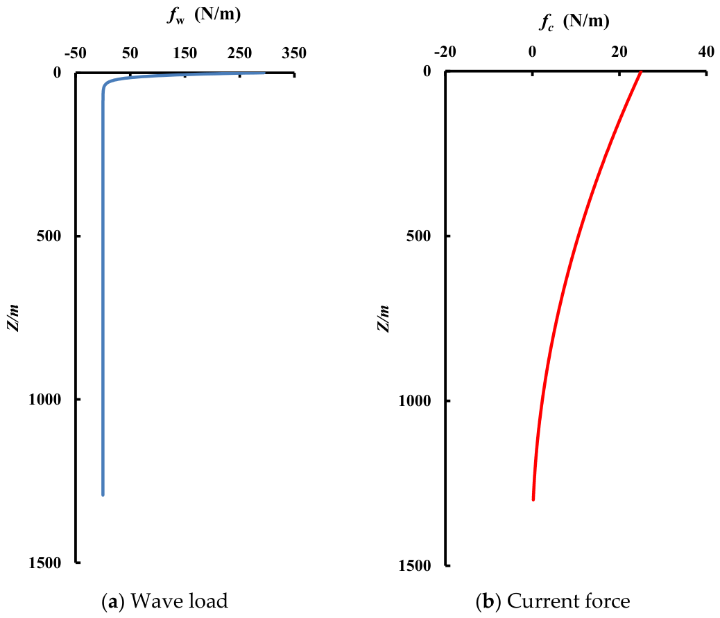
As shown in Figure 10, the wave load changes periodically with time. Therefore, the wave load $f_w$(0) reaches the largest value of 294.39 N when t = 0.11 + T, which could be used as the distributed force of the wave load. Then, the wave load and current force varying with the calculation depth of sea can be obtained from Equations (31) and (32), as shown in Figure 11.

Figure 10. Variation in wave load on sea surface.

Figure 11. Variation in wave load and current with depth.

First, assuming that there is no lateral offset between moon pool O and wellhead A, the torque at end $P_0$, the axis force at end $P_L$, and the angle between the wave load and the current force are all known. The required parameters are listed in Table 10.

Table 10. Calculation parameters of landing string.

Parameters	Symbol	Value	Units
Coordinates of end $P_0$	$X_0$	0.00	m
	$Y_0$	0.00	m
	$Z_0$	0.00	m
Torque on end $P_0$	$M_{03}$	15.00	kN·m
Euler quaternions on end $P_L$	$q_{L1}$	0.00	-
	$q_{L2}$	1.00	-
	$q_{L3}$	0.00	-
	$q_{L4}$	0.00	-
Coordinates of end $P_L$	$X_L$	0.00	m
	$Y_L$	0.00	m
Axis force on end $P_L$	$F_{L3}$	600.00	kN
Angle between wave load and current force	$\beta$	90.00	°
Units of landing string	n	650.00	-

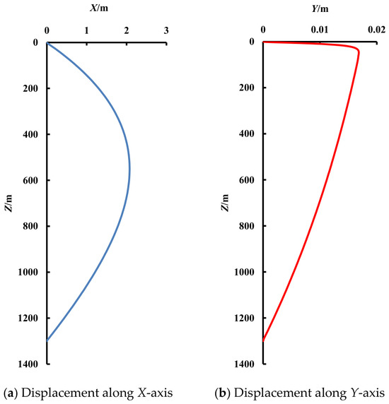
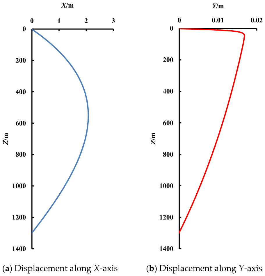
The parameters in Table 6 and Table 8 are introduced into the closed equations for the landing string, and then the deformation and force of the landing string influenced by the wave load and current force are obtained. The deformation of the landing string can be expressed by the lateral displacements of each node in the fixed coordinate system O-XYZ, as shown in Figure 12.

Figure 12. Lateral displacements of landing string.

From Figure 12, the lateral displacement in the X-axis is much greater than that in the Y-axis, which means that the current force is the main reason for the deformation of the landing string. Meanwhile, the wave load is only distributed along approximately 30 m of the sea surface and has little effect on the deformation of the landing string.

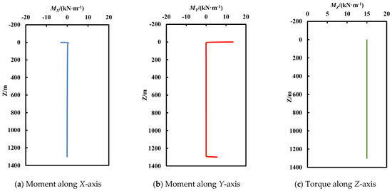
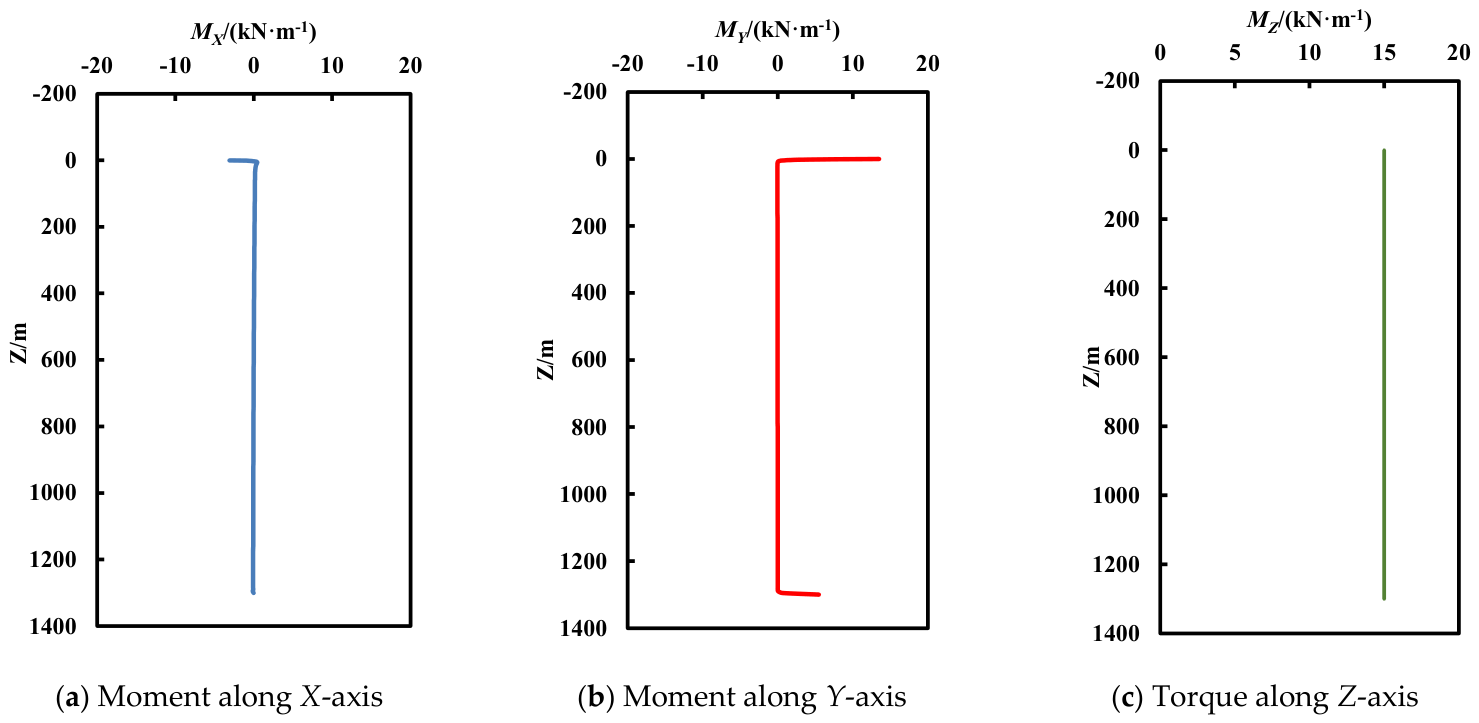
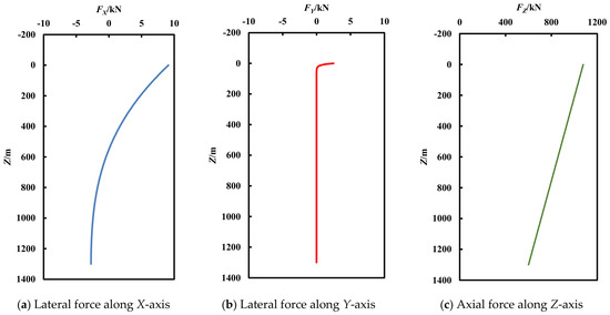
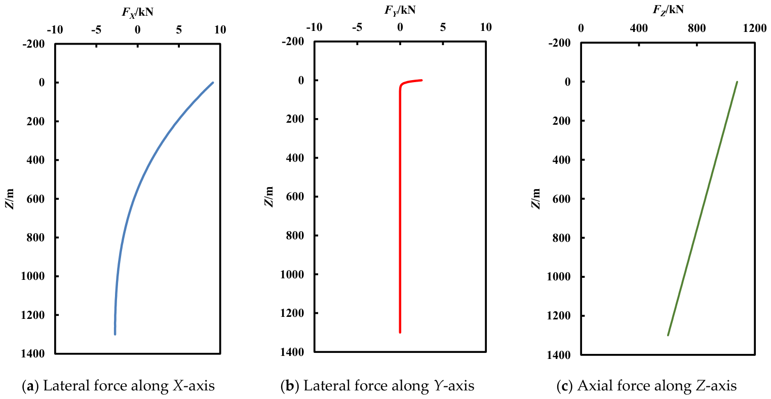
The components of forces and moments at all nodes can be converted from the principal axis coordinate system to the fixed coordinate system, as shown in Figure 13 and Figure 14.

Figure 13. Moments of landing string.

Figure 14. Force of landing string.

From Figure 14 and Figure 15, the maximum lateral force, axial force, and bending moment are all at end $P_0$, in which accidents of overload tension and shear failure occur easily. The Mises stress at end $P_0$ can be used to evaluate the failure risk for a landing string, as indicated in Equation (39).

$${\sigma }_{\mathrm{Mises}}=\sqrt{{\left(\left|{\displaystyle \frac{F_{03}}{S}}\right|+{\displaystyle \frac{D_o\sqrt{M_{01}^{ 2}+M_{02}^{ 2}}}{2I_A}}\right)}^2+3{\left({\displaystyle \frac{\sqrt{F_{01}^{ 2}+F_{02}^{ 2}}}{S}}\right)}^2+3{\left({\displaystyle \frac{M_{03} D_o}{2I_Z}}\right)}^2}$$

(39)

where S is the cross-sectional area of the landing string (${\mathrm{m}}^2$), $I_A$ is the inertia moment of cross-section (${\mathrm{m}}^4$), and $I_Z$ is the polar inertia moment of cross-section (${\mathrm{m}}^4$). Therefore, the forces and moments on end $P_0$ can be unified into a parameter using Equation (39), and higher Mises stress indicates greater failure risk of the landing string.

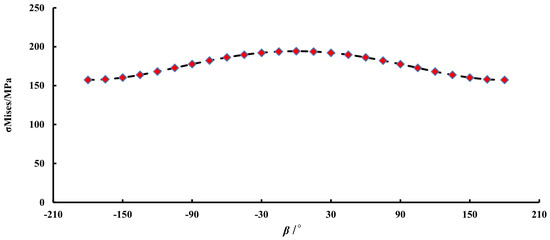
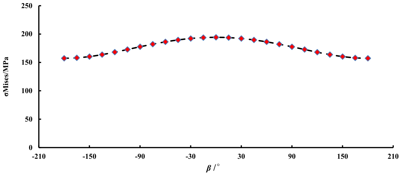
Figure 15. Effect of angle between current force and wave load on Mises stress of end $P_0$.

Second, the angle between the current force and wave load $\beta$ ranges from −180° to 180°, whereas the rest of the parameters are not changed. The effect of different angles on the Mises stress is analyzed, and the results are illustrated in Figure 15.

From Figure 15, the angle between the current force and wave load $\beta$ has an influence on the Mises stress at end $P_0$. The Mises stress increases with the decrease in angle $\beta$, reaching a maximum value of 194.30 Mpa when $\beta$= 0°, and reaches the minimum value of 157.34 Mpa when $\beta$ = 180°. Therefore, the risk failure of the landing string will decrease with an increase in the angle between the wave load and current force.

Finally, the influence of the platform offset on the Mises stress of end $P_0$ is analyzed further. As shown in Figure 16, it is assumed that the positions of the fixed coordinate system O-XYZ and the wellhead at point A remain unchanged. The platform can move in the plane composed of the X-axis and Y-axis by changing the new position of the moon pool $O^{\prime }$. Then, the relative position of the two ends on the landing string can be controlled. The coordinates of point $O^{\prime }$ are marked as $X_{O^{\prime }}$ and $Y_{O^{\prime }}$.

Figure 16. Relationship of direction between offset of platform and wave load or current force.

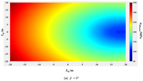
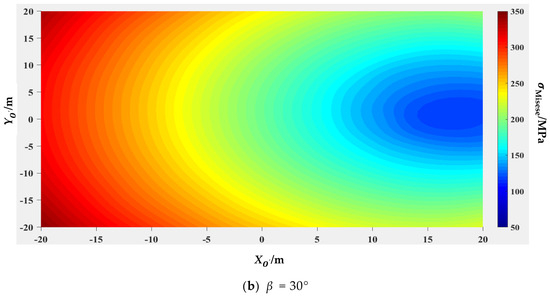
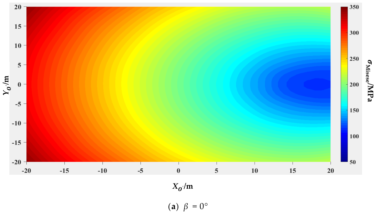
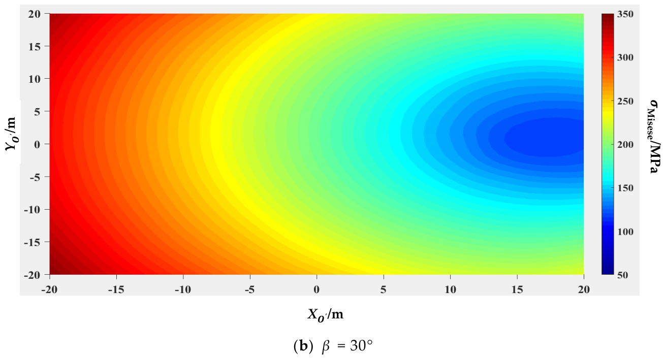
The coordinates of point $O^{\prime }$ are changed from $X_{O^{\prime }}$= −20 m, $Y_{O^{\prime }}$= −20 m to $X_{O^{\prime }}$= 20 m, $Y_{O^{\prime }}$= 20 m, whereas the selections of $\beta$ are 0° and 30°, respectively. The effects of platform offset on the Mises stress at end $P_0$ are illustrated in Figure 17.

Figure 17. Changing regularity of platform offset affecting Mises stress.

Figure 17 shows that Mises stress ${\sigma }_{\mathrm{Mises}}$ will change significantly with the position of the platform. As shown in Figure 17a, when the angle between the current force and wave load is 0°, Mises stresses are symmetrically distributed on both sides of $Y_{O^{\prime }}$ = 0. In addition, when the platform shifts in the same direction with the current force, the Mises stress will decrease with the increase in platform offset and reach the minimum value of 114.80 MPa at $X_{O^{\prime }}$ = 18 m, $Y_{O^{\prime }}$ = 0 m. As shown in Figure 17b, when the angle between the current force and wave load is 30°, although the area with less Mises stresses moves over the positive direction of the Y-axis moderately, the Mises stress will significantly decrease with the platform shifting in the same direction with the current force and reach the minimum value of 106.10 MPa at $X_{O^{\prime }}$ = 17 m, $Y_{O^{\prime }}$ = 1.5 m. Thus, it can be concluded that controlling the offset of the platform along the direction of the current force can effectively reduce the stress on the landing string, thereby reducing the safety risk during drilling.

Thus far, the introduction of the application of the single-span elastic rod model in deep-water drilling has been completed, and it mainly includes force analysis, set of boundary condition, exertion of distributed force, and example calculation. This model can reasonably explain the influence of different factors on the landing string. The use of this model is an extension of deep-water drilling from two-dimensional to three-dimensional, and also a preliminary attempt in a new engineering application area.

6. Conclusions

To establish a comprehensive static method for a single-span elastic rod based on the nonlinear mechanical theory of elastic rods, this paper discusses several key issues in the establishment of the model, such as degree of freedom, boundary condition, calculation method, model verification, and procedure of application.

There are 24 boundary parameters on the ends of an elastic rod, including the principal vector components, principal moment components, Euler angles, and coordinate components. Among them, the number of independent parameters is only 12; thus, the elastic rod’s degree of freedom is 12. To make the system of a single-span elastic rod closed, it is necessary to find the boundary condition consisting of 12 boundary parameters.

The boundary condition can be divided into generalized displacement and generalized force; they have a one-to-one correspondence in a certain direction and cannot be simultaneously given. To determine the deformation, attitude, and position of the single-span elastic rod entirely, there must be at least six generalized displacements at the two ends. Thus, there are seven types of boundary conditions that could entirely determine the deformation, attitude, and position of the elastic rod, and the total number for the seven types is 729.

The elastic rods can become two-dimensional circular rods and three-dimensional helical rods by setting the boundary conditions and using the calculation of the discrete method. Meanwhile, two mathematical curves corresponding to the circular rod and helical rod are established to verify the rationality of this method. The results show that the discrete method for the single-span elastic rod model is accurate, and the single-span elastic rod model can be used to solve the rod with large deformation.

The deep-water landing string example in Section 5 is intended as a methodological demonstration of the application procedure; for real engineering design, additional site-specific factors and more detailed validation would be required [50,51,52]. Beyond deep-water landing strings, the proposed single-span elastic rod model can be applied to several other domains with specific details. In petroleum engineering, it enables calculation of critical buckling loads and contact force distribution for drill strings in complex well trajectories, as well as fast assessment of time-varying stresses in riser-less drilling induced by waves and currents. In soft robotics, it facilitates shape reconstruction and precise end-effector positioning of continuum manipulators. For space structures, it can simulate the deployment process of deployable antenna trusses. In ocean engineering, it supports large-deformation static analysis of mooring lines and submarine power cables.

References

- Hibbeler, R.C. Statics and Mechanics of Materials, 2nd ed.; Pearson Schwz Ag: Cham, Switzerland, 2011. [Google Scholar]
- Beer, F.P.; Johnston, E.R.; Dewolf, J.T. Statics and Mechanics of Materials; China Machine Press: Beijing, China, 2014. [Google Scholar]
- Bai, J.Z.; Lin, X.M. Two-dimensional analysis of bottom hole assembly by beam-column theory. Acta Pet. Sin. 1985, 6, 75–84. [Google Scholar]
- Su, Y.N.; Tang, X.P.; Chen, Z.X. Equivalent loading method for solving beam-column with initial bending and its application in drilling engineering. Mech. Eng. 2004, 26, 42–44. [Google Scholar]
- Shi, Y.M.; Hearst, J.E. The Kirchhoff elastic rod, the nonlinear Schrödinger equation, and DNA supercoiling. J. Chem. Phys. 1994, 101, 5186–5200. [Google Scholar] [CrossRef] [Scilit]
- Carrera, E.; Giunta, G.; Petrolo, M. Beam Structures: Classical and Advanced Theories; John Wiley & Sons: Chichester, UK, 2011. [Google Scholar]
- Antman, S.S. The theory of rods. In Handbuch der Physik, Vol. Via/2, Mechanics of Solids II; Truesdell, C., Ed.; Springer: Berlin/Heidelberg, Germany, 1972; pp. 641–703. [Google Scholar]
- Ilyukhin, A.A. Spatial Problems of the Nonlinear Theory of Elastic Rods; Naukova Dumka: Kiev, Ukraine, 1979. (In Russian) [Google Scholar]
- Liu, Y.Z. Nonlinear Mechanics of Thin Elastic Rod—Theoretical Basic of Mechanical Model of DNA; Tsinghua University Press: Beijing, China, 2006. (In Chinese) [Google Scholar]
- Kehrbaum, S.; Maddocks, J.H. Elastic rods, rigid bodies, quaternions and the last quadrature. Philos. Trans. R. Soc. Lond. A 1997, 355, 2117–2136. [Google Scholar] [CrossRef] [Scilit]
- Nizette, M.; Goriely, A. Towards a classification of Euler-Kirchhoff filaments. J. Math. Phys. 1999, 40, 2830–2866. [Google Scholar] [CrossRef] [Scilit]
- Healey, T.J.; Mehta, P.G. Straightforward computation of spatial equilibria of geometrically exact Cosserat rods. Int. J. Bifurc. Chaos 2005, 15, 949–965. [Google Scholar] [CrossRef] [Scilit]
- Xue, Y.; Liu, Y.Z.; Chen, L.Q. Methods of analytical mechanics for dynamics of the Kirchhoff elastic rod. Acta Phys. Sin. 2006, 55, 3845–3851. [Google Scholar] [CrossRef] [Scilit]
- Kawakubo, S. Kirchhoff elastic rods in three-dimensional space forms. J. Math. Soc. Jpn. 2008, 60, 551–582. [Google Scholar] [CrossRef] [Scilit]
- Jung, P.; Leyendecker, S.; Linn, J.; Ortiz, M. A discrete mechanics approach to the Cosserat rod theory-Part 1: Static equilibria. Int. J. Numer. Methods Eng. 2011, 85, 31–60. [Google Scholar] [CrossRef] [Scilit]
- Goicoechea, H.E.; Buezas, F.S.; Rosales, M.B. A non-linear Cosserat rod model for drill-string dynamics in arbitrary borehole geometries with contact and friction. Int. J. Mech. Sci. 2019, 158, 98–110. [Google Scholar] [CrossRef] [Scilit]
- Goicoechea, H.E.; Lima, R.; Buezas, F.S.; Sampaio, R. Drill-string with cutting dynamics: A mathematical assessment of two models. J. Sound Vib. 2023, 544, 117364. [Google Scholar] [CrossRef] [Scilit]
- Goicoechea, H.E.; Lima, R.; Sampaio, R. How to mathematically model a drill-string: Lumped or continuous models? Chaos Solitons Fractals 2024, 188, 115543. [Google Scholar] [CrossRef] [Scilit]
- Goicoechea, H.E.; Lima, R.; Buezas, F.S.; Sampaio, R. A comprehensive Cosserat rod drill-string model for arbitrary well geometry that includes the dynamics of the cutting and lateral contact. J. Sound Vib. 2024, 571, 118035. [Google Scholar] [CrossRef] [Scilit]
- Yu, F.; Huang, G.L.; Han, Z.Y.; NI, H.; Li, J.; Li, W. Method of suspender line trajectory design. Pet. Explor. Dev. 2021, 48, 1208–1217. [Google Scholar] [CrossRef] [Scilit]
- Jun, G.; Zhi, X.D.; Fan, F.; Shen, S.Z. Static and dynamic stiffness in the modeling of inclined suspended cables. J. Constr. Steel Res. 2020, 172, 106210. [Google Scholar] [CrossRef] [Scilit]
- Xie, D.; Huang, Z.Q.; Ma, Y.C.; Vaziri, V.; Kapitaniak, M.; Wiercigroch, M. Nonlinear dynamics of lump mass model of drill-string in horizontal well. Int. J. Mech. Sci. 2020, 174, 105450. [Google Scholar] [CrossRef] [Scilit]
- Li, W.; Huang, G.L.; Yu, F.; Ni, H.; Jiang, W.; Zhang, X. Modeling and numerical study on drillstring lateral vibration for air drilling in highly-deviated wells. J. Pet. Sci. Eng. 2020, 195, 107913. [Google Scholar] [CrossRef] [Scilit]
- Yu, F.; Huang, G.L.; Ni, H.J.; Nie, Z.; Li, W.; Li, J.; Jiang, W. Analysis of the main factors affecting bottom hole assembly Re-entry into main hole in forward drilling of fishbone wells. J. Pet. Sci. Eng. 2020, 189, 107018. [Google Scholar] [CrossRef] [Scilit]
- Chen, B.; Huang, J.; Ji, J.C. Control of flexible single-link manipulators having duffing oscillator dynamics. Mech. Syst. Signal Process. 2019, 121, 44–57. [Google Scholar] [CrossRef] [Scilit]
- Artinian, A.; Ben Amar, F.; Perdereau, V. Closed-loop shape control of deformable linear objects based on Cosserat model. IEEE Robot. Autom. Lett. 2024, 9, 8746–8753. [Google Scholar] [CrossRef] [Scilit]
- Pourghasemi Hanza, S.; Ghafarirad, H. Mechanics of fiber-reinforced soft manipulators based on inhomogeneous Cosserat rod theory. Mech. Adv. Mater. Struct. 2024, 31, 3161–3173. [Google Scholar] [CrossRef] [Scilit]
- Guan, Z.C.; Li, J.J.; Han, C.; Zhang, B.; Zhao, X.F. Loads calculation and strength analysis of landing string during deepwater drilling. J. China Univ. Pet. (Ed. Nat. Sci.) 2018, 42, 77–84. [Google Scholar]
- Liu, Y.Z.; Xue, Y. Qualitive analysis of supercoiling configuration of a thin elastic rod under tension and twist. Acta Phys. Sin. 2009, 58, 5936–5941. [Google Scholar] [CrossRef] [Scilit]
- Xue, Y.; Zhang, Y. Mechanical Model of Super-thin Elastic Rod and Boundary Conditions. J. Appl. Eng. Sci. 2007, 25, 306–310. [Google Scholar]
- Armero, F. A new Hermite finite element for nonlinear Kirchhoff rods: The plane case. Int. J. Numer. Methods Eng. 2024, 125, 7448. [Google Scholar] [CrossRef] [Scilit]
- Harsch, J.; Sailer, S.; Eugster, S.R. A total Lagrangian, objective and intrinsically locking-free Petrov–Galerkin SE(3) Cosserat rod finite element formulation. Int. J. Numer. Methods Eng. 2023, 124, 2965–2994. [Google Scholar] [CrossRef] [Scilit]
- Vu-Quoc, L.; Humer, A. Partial-differential-algebraic equations of nonlinear dynamics by physics-informed neural-network. I: Operator splitting and framework assessment. Int. J. Numer. Methods Eng. 2024, 125, e7586. [Google Scholar] [CrossRef] [Scilit]
- Gatti-Bono, C.; Perkins, N.C. Numerical simulations of cable/seabed interaction. Int. J. Offshore Polar Eng. 2004, 14, 118–124. [Google Scholar]
- Goss, V.G.A.; Van der Heijden, G.H.M.; Thompson, J.M.T. Experiments on snap bucking, hysteresis and loop formation in twisted rods. Exp. Mech. 2005, 45, 101–111. [Google Scholar] [CrossRef]
- Du, H.W. Physical Modeling and Configuration Simulation for Flexible Cable. Master’s Thesis, Dalian Maritime University, Dalian, China, 2015. [Google Scholar]
- Ma, G. Dynamics Study of Deepwater Mooring Line and Riser Based on Elastic Rod Theory. Ph.D. Thesis, Harbin Engineering University, Harbin, China, 2009. [Google Scholar]
- Veseth, P.A. On the Use of a New Mathematical Formulation for Loads- and Motion Analysis of a Mooring Line. Master’s Thesis, University of Bergen, Bergen, Norway, 2023. [Google Scholar]
- O’Reilly, O.M. Modeling nonlinear problems in the mechanics of strings and rods. In The Role of the Balance Laws, 1st ed.; Springer: Cham, Switzerland, 2017. [Google Scholar]
- Arora, A.; Kumar, A.; Steinmann, P. A computational approach to obtain nonlinearly elastic constitutive relations of special Cosserat rods. Comput. Methods Appl. Mech. Eng. 2019, 350, 295–314. [Google Scholar] [CrossRef] [Scilit]
- de Miguel, A.G.; De Pietro, G.; Carrera, E.; Giunta, G.; Pagani, A. Locking-free curved elements with refined kinematics for the analysis of composite structures. Comput. Methods Appl. Mech. Eng. 2018, 337, 481–500. [Google Scholar] [CrossRef] [Scilit]
- Xue, Y. Modeling and Analysis of Nonlinear Mechanics of a Super-Thin Elastic Rod. Ph.D. Thesis, Shanghai University, Shanghai, China, 2004. [Google Scholar]
- Krasilnikov, P.S. On a discrete model of the elastic rod. Int. J. Nonlinear Ences Numer. Simul. 2001, 2, 295–298. [Google Scholar] [CrossRef] [Scilit]
- Kapitaniak, M.; Vaziri, V.; Wiercigroch, M. Bifurcation scenarios in helical buckling of slender rods using new FE. Int. J. Eng. Sci. 2020, 147, 103197. [Google Scholar] [CrossRef] [Scilit]
- Banan, M.R.; Karami, G.; Farshad, M. Finite element analysis of curved beams on elastic foundations. Comput. Struct. 1989, 32, 45–53. [Google Scholar] [CrossRef] [Scilit]
- da Fonseca, A.F.; de Aguiar, M.A.M. Solving the boundary value problem for finite Kirchhoff rods. Phys. D. Nonlinear Phenom. 2002, 181, 53–69. [Google Scholar] [CrossRef] [Scilit]
- Zhou, S.L.; Cong, Y.C.; Li, J.; Dai, H.D. Comparison of algorithms for extracting quaternion from DCM. J. Chin. Inert. Technol. 2008, 16, 41–44. [Google Scholar]
- Williamson, C.H.K. In-line response of a cylinder in oscillatory flow. Appl. Ocean. Res. 1985, 7, 97–106. [Google Scholar] [CrossRef] [Scilit]
- Bordet, L.; Franchi, J.; Granger, S. Innovative forging process allows safer and cost effective heavy duty landing string for deepwater applications. In Proceedings of the SPE Deepwater Drilling and Completions Conference, Galveston, TX, USA, 14–15 September 2016. [Google Scholar]
- Tian, L.; Zhang, Q.; Li, X.; Li, C. Fracturing Effectiveness Evaluation Based on Flowback Data Using Pressure Transient Testing. Reserv. Sci. 2026, 2, 97–110. [Google Scholar] [CrossRef] [Scilit]
- Ali, J.; Ansari, U.; Ali, F.; Javed, T.; Hullio, I.A. Application of Machine Learning for Effective Screening of Enhanced Oil Recovery Methods. Reserv. Sci. 2026, 2, 65–80. [Google Scholar] [CrossRef] [Scilit]
- Hu, Y.; Yang, Y. A Comparative Study on Drag Reduction Methods for Continental Shale Drilling in the Fuxing Block, Southeastern Sichuan Basin. Reserv. Sci. 2026, 2, 81–96. [Google Scholar] [CrossRef] [Scilit]
Disclaimer/Publisher’s Note: The statements, opinions and data contained in all publications are solely those of the individual author(s) and contributor(s) and not of MDPI and/or the editor(s). MDPI and/or the editor(s) disclaim responsibility for any injury to people or property resulting from any ideas, methods, instructions or products referred to in the content. |
© 2026 by the authors. Licensee MDPI, Basel, Switzerland. This article is an open access article distributed under the terms and conditions of the Creative Commons Attribution (CC BY) license.