3D DL-Based Surrogate Modeling for Borehole Resistivity Inversion in Anisotropic Formations

Abstract

To address the low computational efficiency of conventional forward modeling that hinders real-time inversion of borehole resistivity logging data in deviated/horizontal wells through anisotropic formations, this paper presents an adaptive inversion method based on a deep neural network forward surrogate model. A resistivity response database covering deviation angle, mud invasion, and anisotropy is constructed using three-dimensional finite-element forward modeling. The deep neural network architecture is systematically optimized by varying the number of hidden layers and neurons per layer, comparing five activation functions, evaluating four training algorithms, and testing five batch size ratios. The resulting deep learning-based forward model achieves a speedup of over two orders of magnitude compared with 3D finite-element modeling while maintaining high accuracy (maximum relative error < 1%). By integrating this fast forward model with an adaptively modified Levenberg–Marquardt algorithm, rapid inversion in anisotropic formations is realized. Numerical simulations and field data processing demonstrate that the proposed method accurately extracts uninvaded resistivity, invasion depth, and anisotropy coefficient, with an efficiency gain of approximately 98% over traditional approaches. Reconstructed logs show excellent agreement with measured data, providing robust support for real-time evaluation of deviated and horizontal wells.

1. Introduction

With the continuous growth in global demand for oil and gas resources, exploration focus has shifted toward unconventional reservoirs such as tight sandstones and shale formations. These reservoirs typically exhibit poor porosity properties with high development costs [1,2,3,4]. Therefore, deviated/horizontal well technology is employed. The key advantage of this approach lies in significantly increasing the contact area between the borehole and the target reservoir, thereby substantially improving both well productivity and recovery [5,6]. Currently, most oil fields worldwide, particularly shale oil and gas reservoirs, are increasingly deploying horizontal wells to enhance production efficiency. In well logging evaluation, resistivity is a critical parameter for identifying hydrocarbon potential. However, electrical anisotropy is commonly induced by grain alignment, pervasive oriented fractures, and layered structures, causing the measured apparent resistivity to significantly deviate from the true formation resistivity [7,8,9,10]. As a result, accurate evaluation of resistivity in anisotropic formations has become a key challenge for reservoir characterization.

Geophysical inversion is essential for accurately estimating anisotropic resistivity parameters. At present, the most widely used inversion methods in electrical logging fall into two main categories: stochastic and deterministic algorithms [11,12,13]. Stochastic algorithms (e.g., particle swarm optimization, simulated annealing, differential evolution) perform global random searches and offer strong multi-parameter optimization capabilities, although they are often computationally expensive. Deterministic algorithms (e.g., Gauss–Newton, Levenberg–Marquardt) are rooted in least-squares theory and iteratively adjust model parameters to minimize the misfit between simulated and measured data, and their fast convergence and robust mitigation of environmental effects have made them widely adopted in electrical logging inversion in recent years [14,15,16,17].

Although deterministic algorithms are widely used for fast processing of electrical logging data, they have notable limitations when applied to anisotropic formations. In such cases, inversion typically requires three-dimensional (3D) forward modeling. Taking the 3D finite element method (3D-FEM) as an example, high accuracy comes at the cost of extremely fine meshes—often containing tens of thousands to millions of elements—resulting in very low computational efficiency that precludes real-time or rapid log evaluation [18,19,20]. In current field data practice, direct current electrical logging data are processed using a point-by-point inversion approach. Consider a 100 m well interval sampled at 0.1 m spacing (total of 1001 logging points). A standard gradient-based inversion requires at least five iterations per point, with each iteration involving six forward simulations and Jacobian computation. Given that each 3D-FEM forward simulation takes about 0.7 s, the total computational time amounts to roughly 21,021 s (5.84 h). Such a heavy computational burden severely limits interpretation efficiency, highlighting the critical need for faster forward modeling.

Recently, deep learning (DL) has been introduced into geophysical inversion to overcome the low efficiency of forward modeling in conventional workflows [21]. Through offline training, it constructs a rapid nonlinear mapping from model parameters to logging responses, enabling the replacement of costly 3D numerical forward modeling with near-real-time computation during inversion [22,23,24,25,26]. For example, Xu et al. used DL methods to achieve rapid and accurate reconstruction of electromagnetic wave logging-while-drilling responses [27]. By comparing neural networks, gradient-boosted regression trees, and Gaussian process regression, they clearly demonstrated the high efficiency of DL in forward modeling. Raissi et al. employed deep neural networks to accelerate the solution of partial differential equations, achieving substantial efficiency improvements over conventional numerical methods [28]. Paszynski et al. replaced the original iterative algorithm in the hp-adaptive finite element method with a deep neural network framework, enabling automatic optimization of mesh element count and interpolation polynomial order [29]. This approach significantly enhanced both the speed and accuracy of numerical simulations. Collectively, these studies indicate that deep learning-based forward surrogate models represent a highly promising pathway for fast resistivity inversion in anisotropic formations.

Although the application of DL in well logging is still in its early stages, preliminary results already show its potential to meet practical demands. effectively incorporating intelligent algorithms into fast forward modeling for logging presents two core challenges that must be addressed: (1) High-quality, representative resistivity responses databases are essential to fully exploit the learning capacity of deep neural networks. For anisotropic formations and deviated/horizontal wells, training samples must span a wide range of key parameters—e.g., anisotropy coefficients, deviation angles, and layer resistivity. Inadequate or imbalanced sample coverage seriously degrades the generalization performance of the surrogate model. (2) Neural network architecture design: DL models, particularly fully connected networks, involve a large number of trainable parameters, yet there is no standardized procedure for optimizing their structure (e.g., number of layers, neurons, activation functions). Effectively addressing these two challenges is essential for realizing deep learning-based surrogates for 3D forward modeling.

To address these challenges, this paper presents a technical strategy for anisotropic inversion of array resistivity logging in deviated/horizontal wells. First, a 3D resistivity response database is generated by 3D finite-element (3D-FEM) forward modeling, considering deviation angle, mud invasion, and anisotropy, to provide reliable training data for deep neural networks. Second, the effects of network depth, activation functions, and optimization algorithms on predictive performance are systematically analyzed, leading to the design of an efficient deep neural network surrogate model. The prediction accuracy and computational efficiency of this model are subsequently validated. Finally, an adaptive modified Levenberg–Marquardt algorithm is employed to construct a fast resistivity inversion method for anisotropic formations with deviated/horizontal wells. The reliability of the inversion scheme is validated through numerical simulation examples, and the method is further applied to field data processing to assess its performance.

2. Deep Learning-Based Forward Model

2.1. Fast Forward Modeling Method

2.1.1. Borehole Resistivity Response Database Construction

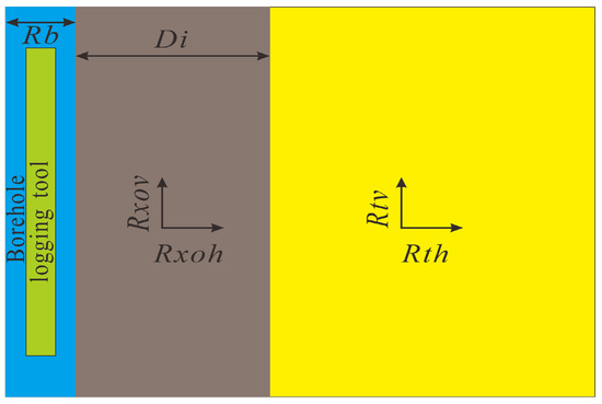
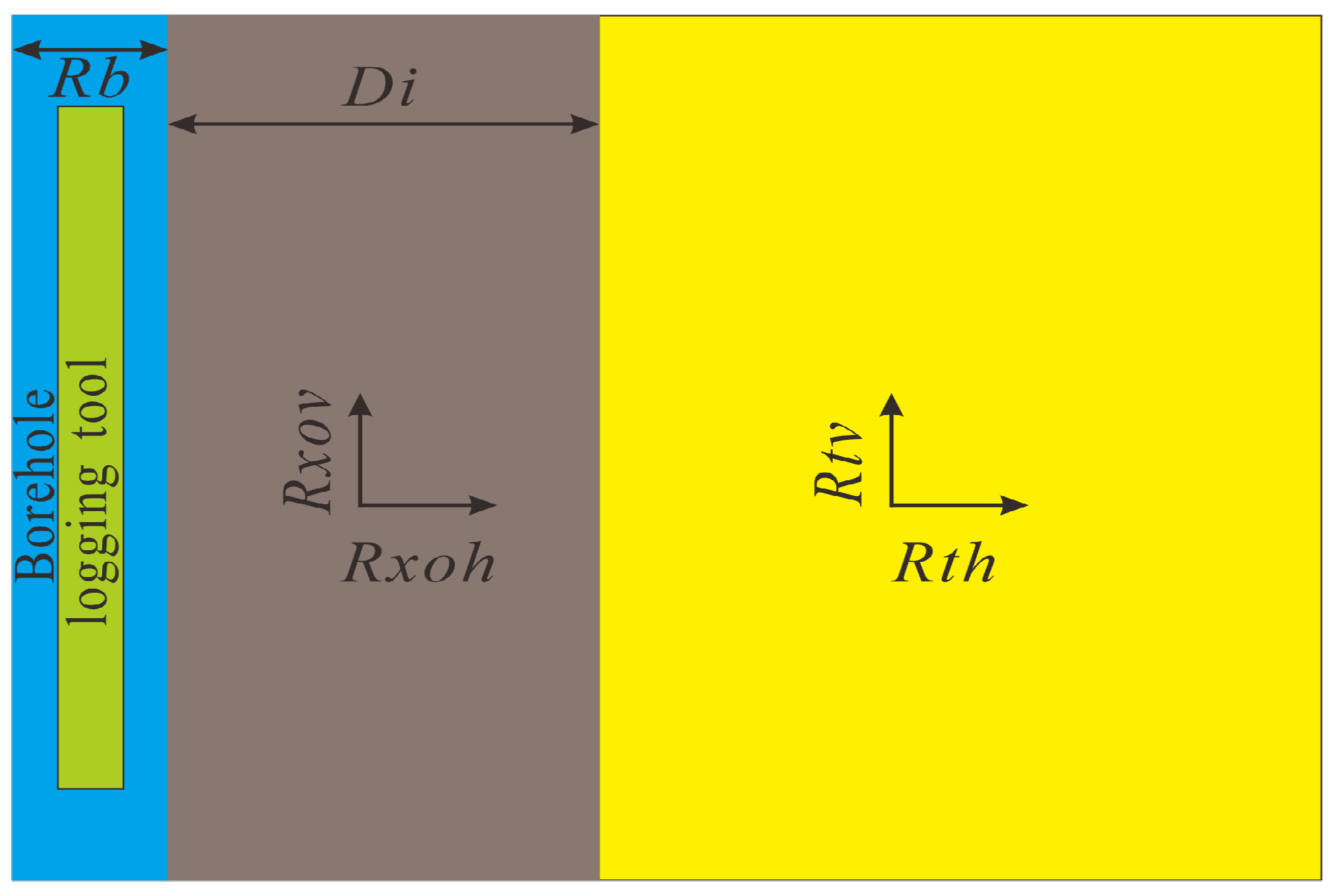
As an inherently data-driven learning mechanism, the deep learning framework relies on a comprehensive and representative response database to ensure that prediction results meet accuracy requirements [30]. The High Resolution Laterolog Array (HRLA) instrument developed by Schlumberger (Houston, TX, USA) is taken as an example in this paper. In borehole resistivity logging (a post-drilling measurement), mud invasion effects are non-negligible. Moreover, for shale, sandy mudstone, and carbonate formations in deviated wells, both deviation angle and formation anisotropy play important roles. Collectively, the dominant parameters governing borehole resistivity responses encompass borehole diameter (Rb), mud resistivity (Rm), deviation angle (θ), invasion depth (Di), the horizontal resistivities of both the invaded and virgin zones (Rxoh and Rth), as well as formation anisotropy ($\lambda =\sqrt{{\displaystyle \raisebox{1ex}{$Rtv$}\!\left/ \!\raisebox{-1ex}{$Rth$}\right.}}$). The corresponding formation model is schematically depicted in Figure 1.

Figure 1. Formation model for generating response database.

After fixing the model, parameters are sampled within specified bounds, with the deviation angle θ varying from 0° to 90°. To improve network fitting capability, avoid gradient vanishing, and reduce errors, the θ range is divided into 10 intervals, each serving as the basis for a separate sub-database. Thus, the entire resistivity response database comprises 10 sub-databases. Table 1 lists the sampling ranges of the parameters for each sub-database. Rat is the ratio of invaded-zone to virgin-zone horizontal resistivity. Moreover, resistivity values are expressed on a logarithmic scale. All parameter combinations were generated using a full factorial grid sampling strategy based on the discrete values listed in Table 1.

Table 1. Range of parameters in resistivity response database.

Parameter	rb/in.	Log (Rm)/Ω·m	Di/m	Log (Rxoh)/Ω·m	Rat	λ
Range	6~12	−2~−1	0~1	−1~3	1~20	1~5
Group	5	4	10	20	21	6

According to the parameter combinations listed in Table 1, each sub-database contains 5 × 4 × 10 × 20 × 21 × 6 = 504,000 samples. Each sample comprises six model parameters, yielding a total of 504,000 parameter sets, which are stored in variable M as a matrix of size 504,000 × 6. Then, the 3D finite-element forward modeling, which was employed in this study, follows the numerical scheme established in our previous work (Wu & Fan, 2021) [31] and is adopted to generate the resistivity response database. Concurrently, each sample produces five apparent resistivity values (RLA1–RLA5) [32], resulting in a total of 504,000 × 5 = 2,520,000 data points. These are stored as output in variable D with dimensions 504,000 × 5504,000 × 5. Assuming double precision, each matrix occupies about 0.024 GB, and the total size of the entire resistivity response database is approximately 0.24 GB.

To illustrate the data format, fifty sample data are presented (including both input and output parameters) in Appendix A.

2.1.2. Deep Neural Network Framework

In deep learning, the loss function determines the direction and step size of network parameter updates. In this section, the objective function is formulated as the mean squared error (MSE). To mitigate overfitting and enhance the generalization capability of the trained model, an L2 regularization term is added to the MSE loss, which is expressed as follows [33]:

$$L\left(w,b,x\right)={\displaystyle \frac{1}{m}}{\displaystyle \sum _{i=1}^m{\displaystyle \sum _{j=1}^5{\left(g{\left(x,w,b\right)}_j^i-y_j^i\right)}^2}}+{\displaystyle \frac{\chi }{2m}}{‖w,b‖}_2^2$$

(1)

where g is the activation function; w and b are the weights and biases connecting the layers; p is the number of iterations; m is the number of samples; x is the net input vector to the neurons in each layer; y is the output vector of the training set; and $\chi$ is the regularization coefficient.

Prior to feeding the dataset into the deep neural network, min-max normalization is applied to uniformly scale the output data to the [0, 1] range [34]. The normalization formula is given as follows:

$$\left\{\begin{array}{l}{x}_i^{new}={\displaystyle \frac{x_i-x_{i\_min}}{x_{i\_\max }-x_{i\_min}}}\\ y_j^{new}={\displaystyle \frac{lo{g}_{10}\left(y_j\right)-lo{g}_{10}\left(y_{j\_min}\right)}{lo{g}_{10}\left(y_{j\_\max }\right)-lo{g}_{10}\left(y_{j\_min}\right)}}\end{array}\right.$$

(2)

where x_i is the input vector, $x={\left(Rm,rb,Di,Rxo,con,\lambda \right)}^T$, with i = 1,…,6; y is the label vector, y_j = (RLA1, RLA2, RLA3, RLA4, RLA5)^T, with j = 1,…,5, denoting the detection mode; $x_i^{new}$ and $y_i^{new}$ are the normalized data; x_{i_max} and x_{i_min} are the maximum and minimum values of each input parameter, x_{i_max} = (Rm__max, rb__max, Di__max, con__max, λ__max)^T, x_{i_min} = (Rm__min, rb__min, Di__min, con__min, λ__min)^T; y_{j_max} and y_{j_min} are the maximum and minimum values of each resistivity response, y_{j_max} = (RLA1__max, RLA2__max, RLA3__max, RLA4__max, RLA5__max)^T, y_{j_min} = (RLA1__min, RLA2__min, RLA3__min, RLA4__min, RLA5__min)^T.

It is worth noting that the predicted data should be denormalized to revert to the original physical scale.

To fully exploit the learning capability for high-accuracy predictions, a fully connected neural network iteratively updates parameters via backpropagation. Taking a three-layer network as an example, and based on the loss function defined in Equation (1), the forward propagation process is expressed as follows [35]:

$$\left\{\begin{array}{c}{\mathit{z}}^{(1)}={\mathit{W}}^{(1)}\mathit{x}+{\mathit{b}}^{(1)};{\mathit{a}}^{(1)}=f\left({\mathit{z}}^{(1)}\right)\\ z^{(2)}={\mathit{W}}^{(2)}{\mathit{a}}^{(1)}+{\mathit{b}}^{(2)};\widehat{y}={\mathit{a}}^{(2)}=g\left({\mathit{z}}^{(2)}\right)\end{array}\right.$$

(3)

where x is the net input vector to the neurons in each layer, $x={\left(Rm,rb,Di,Rxo,con,\lambda \right)}^T$; ${\mathit{W}}^{(1)}\in {\Re }^{m_1\times d}$, d is the dimension of x, m₁ is the number of neurons in the hidden layer; ${\mathit{W}}^{(2)}\in {\Re }^{m_2\times d}$, m₂ is the number of neurons in the output layer; f and g denote the activation functions of the hidden layer and the output layer, respectively.

Backpropagation, as the name implies, starts from the loss function and adjusts the parameters of preceding layers based on the computed gradients. For a three-layer network, computing the loss gradients with respect to the hidden-to-output weights and biases is essential. As the loss function cannot be directly differentiated with respect to these parameters, the chain rule is applied to derive and compute the derivatives, which are expressed as follows:

$$\left\{\begin{array}{c}{\displaystyle \frac{\partial L}{\partial {\mathit{W}}_i^{(2)}}}={\displaystyle \frac{\partial L}{\partial \widehat{y}}}{\displaystyle \frac{\partial \widehat{y}}{\partial {\mathit{W}}_i^{(2)}}}={\displaystyle \frac{\partial L}{\partial \widehat{y}}}{\displaystyle \frac{\partial \widehat{y}}{\partial g_i}}{\displaystyle \frac{\partial g_i}{\partial {\mathit{W}}_i^{(2)}}}={\displaystyle \frac{\partial L}{\partial \widehat{y}}}{\displaystyle \frac{\partial \widehat{y}}{\partial g_i}}{\displaystyle \frac{\partial g_i}{\partial z_i^{(2)}}}{\displaystyle \frac{\partial z_i^{(2)}}{\partial {\mathit{W}}_i^{(2)}}}\\ {\displaystyle \frac{\partial L}{\partial {\mathit{b}}^{(2)}}}={\displaystyle \frac{\partial L}{\partial \widehat{y}}}{\displaystyle \frac{\partial \widehat{y}}{\partial {\mathit{b}}^{(2)}}}={\displaystyle \frac{\partial L}{\partial \widehat{y}}}{\displaystyle \frac{\partial \widehat{y}}{\partial g_i}}{\displaystyle \frac{\partial g_i}{\partial z_i^{(2)}}}{\displaystyle \frac{\partial z_i^{(2)}}{\partial {\mathit{b}}^{(2)}}}\end{array}\right.$$

(4)

where $\widehat{y}={\displaystyle \sum _{i=1}^{m1}{\mathit{W}}_i^{(2)}{\mathit{a}}_i^{(1)}}+{\mathit{b}}^{(2)}$, g denote the active function.

Finally, Equation (4) can be written as:

$$\left\{\begin{array}{c}{\displaystyle \frac{\partial L}{\partial {\mathit{W}}_i^{(2)}}}=\left(\widehat{y}-y\right)g^{\prime }\left(z_i^{(2)}\right)a_i^{(1)}\\ {\displaystyle \frac{\partial L}{\partial {\mathit{b}}^{(2)}}}=\left(\widehat{y}-y\right)g^{\prime }\left(z_i^{(2)}\right)\end{array}\right.$$

(5)

Equivalent to the following vector form:

$$\left\{\begin{array}{c}{\displaystyle \frac{\partial L}{\partial {\mathit{W}}^{(2)}}}=\left(\widehat{y}-y\right)g^{\prime }\left(z^{(2)}\right){\mathit{a}}^{(1)T}\\ {\displaystyle \frac{\partial L}{\partial {\mathit{b}}^{(2)}}}=\left(\widehat{y}-y\right)g^{\prime }\left({\mathit{z}}^{(2)}\right)\end{array}\right.$$

(6)

where ${\displaystyle \frac{\partial L}{\partial {\mathit{W}}^{(2)}}}\in {\Re }^{1\times m_1}$; ${\displaystyle \frac{\partial L}{\partial {\mathit{b}}^{(2)}}}\in {\Re }^{1\times 1}$.

For a multi-layer neural network, the partial derivatives of the loss function with respect to the weights and biases of the k-th layer are given as follows:

$$\left\{\begin{array}{c}{\displaystyle \frac{\partial L}{\partial W_{ij}^{(k)}}}={\displaystyle \frac{\partial L}{\partial z_i^{(k)}}}{\displaystyle \frac{\partial z_i^{(k)}}{\partial W_{ij}^{(k)}}}={\displaystyle \frac{\partial L}{\partial a_i^{(k)}}}{\displaystyle \frac{\partial a_i^{(k)}}{\partial z_i^{(k)}}}{x}_j\\ {\displaystyle \frac{\partial L}{\partial b_i^{(k)}}}={\displaystyle \frac{\partial L}{\partial z_i^{(k)}}}{\displaystyle \frac{\partial z_i^{(k)}}{\partial b_i^{(k)}}}={\displaystyle \frac{\partial L}{\partial a_i^{(k)}}}{\displaystyle \frac{\partial a_i^{(k)}}{\partial z_i^{(k)}}}\end{array}\right.$$

(7)

where $z_i^{(k)}={\displaystyle \sum _{j=1}^d{W}_{ij}^{(k)}{x}_j+{\mathit{b}}_i^{(k)}}$$a_i^{(k)}$ is the input value of the i-th neuron in the hidden layer, $a_i^{(k)}=f(z_i^{(k)})$, f denotes the activation function.

Finally, using the chain rule, the parameter update formulas for the neural network are obtained as follows:

$$\left\{\begin{array}{c}{\mathit{W}}^{(k)}:={\mathit{W}}^{(k)}-\alpha {\displaystyle \frac{\partial L}{\partial {\mathit{W}}^{(k)}}}\\ {\mathit{b}}^{(k)}:={\mathit{b}}^{(k)}-\alpha {\displaystyle \frac{\partial L}{\partial {\mathit{b}}^{(k)}}}\end{array}\right.$$

(8)

where k indexes the k-th layer of the neural network, and α is the learning rate that determines the update step size during the deep learning process.

2.1.3. Deep Neural Network Training

The layer structure of a deep neural network profoundly influences training accuracy. All neural network training tasks described below were performed on a computer with an Intel Core i9-14900KF CPU and 64 GB RAM. Moreover, the effect of key factors—such as the number of layers, activation function, training algorithm, batch size, and learning rate—on prediction accuracy is task-dependent. Therefore, in this section, these network parameters are optimized using a random subset of 40,000 samples.

The number of layers and neurons fundamentally determines the predictive accuracy of a deep neural network. Thus, we first investigate how these two factors affect training performance. Seven network configurations are built in Table 2, where the listed layer numbers denote only hidden layers.

Table 2. Structure parameters of deep neural network.

No.	The Number of Neural Layers	The Number of Neurons	The Number of Training Parameters
①	1	100	1205
②	2	100/100	11,305
③	3	100/100/100	21,405
④	4	100/100/100/100	31,505
⑤	5	100/100/100/100/100	41,605
⑥	5	100/300/500/300/100	362,405

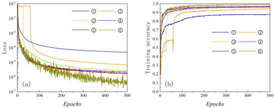
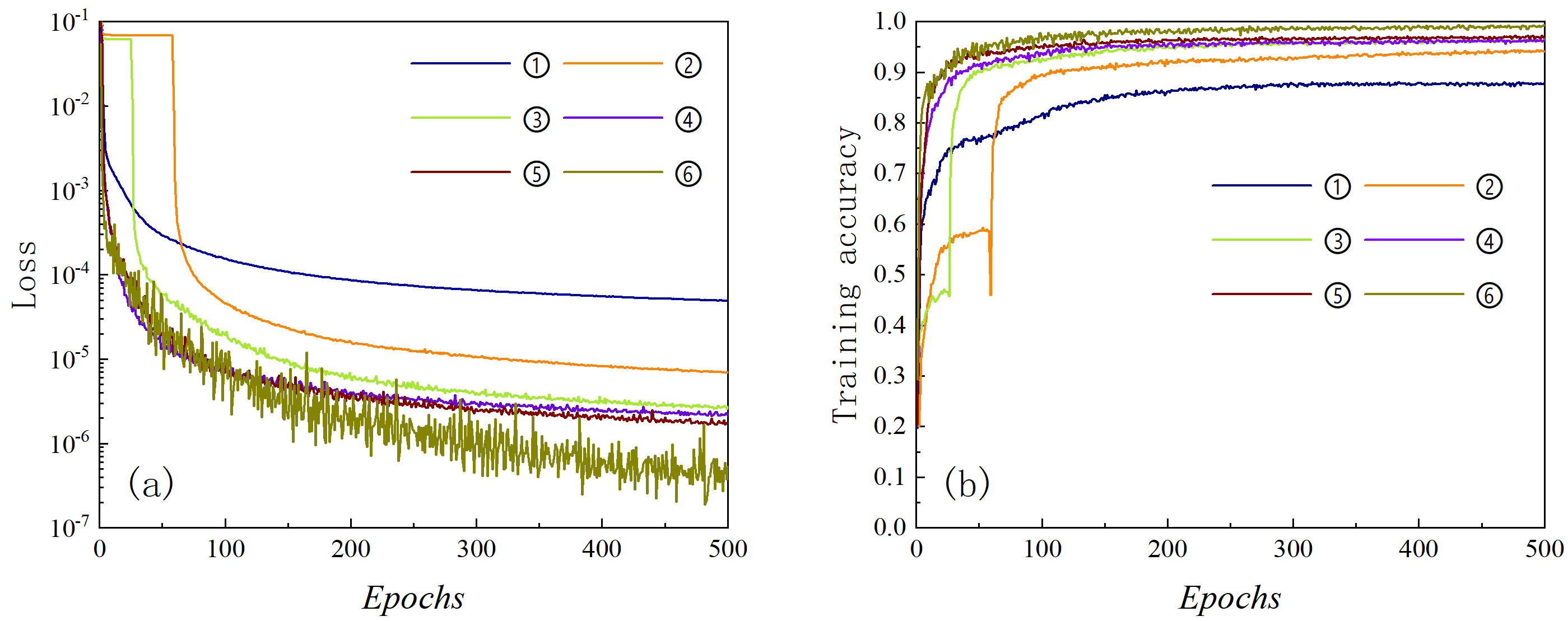
During training, we employ the ReLU activation function and the Adam optimizer. Figure 2 presents the training results for the six neural network models on the small sample dataset. Specifically, Figure 2a,b show the loss function values and training accuracy as functions of the iteration number, respectively. It is evident that with increasing iterations, deeper neural networks consistently outperform shallower ones in terms of training performance. However, beyond a certain layer number, the performance gain gradually saturates, as seen in models ④ and ⑤. Compared with model ④, model ⑤ reduces the loss function value by 17.3% but improves training accuracy by only 0.6%. Adding more network layers would incur substantial computational overhead while providing only marginal improvements in learning performance—an approach that is therefore discouraged.

Figure 2. Training results produced by six neural network structures: (a) loss curve; (b) training accuracy curve.

To further boost training efficiency, we analyze the effect of neuron number. Model ⑥, for instance, has the same layer count as model ⑤ but uses moderately more neurons per layer. As shown in Figure 2, model ⑥ outperforms model ⑤ significantly, reducing the loss function by 75.3% and increasing training accuracy by 3.1%. Consequently, the data-driven network architecture adopted in this paper follows the same layer and neuron configuration as model ⑥.

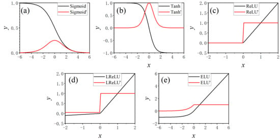
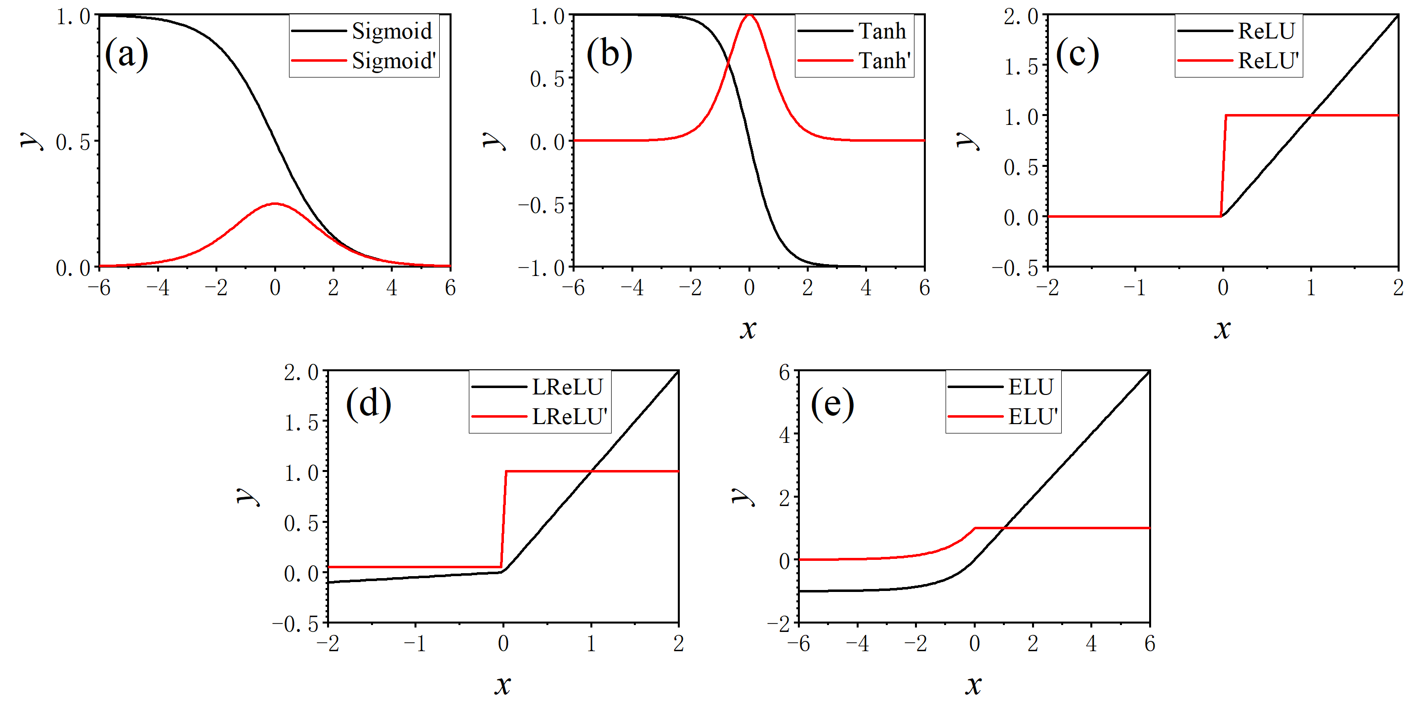
Next, we consider the selection of the activation function. Common candidates include the Sigmoid, Tanh, ReLU, Leaky ReLU (LReLU), and ELU functions. The mathematical expressions are provided in Equations (9)–(12) [36,37].

$$S\left(x\right)={\displaystyle \frac{1}{1+e^x}}$$

(9)

$$\mathrm{Tan}\mathrm{h}\left(x\right)={\displaystyle \frac{e^x-e^{-x}}{e^x+e^{-x}}}=2S(2x)-1$$

(10)

$$\mathrm{Re}\mathrm{LU}\left(x\right)=\left\{\begin{array}{l}x,x>0\\ 0,x\le 0\end{array}\right.$$

(11)

$$\mathrm{LReLU}\left(x\right)=\max \left(nx,x\right)=\left\{\begin{array}{l}x,x>0\\ nx,x\le 0\end{array}\right.$$

(12)

where n is the hyperparameter, and its value is greater than 0.

$$\begin{array}{cc}\mathrm{ELU}\left(x\right)& =\left\{\begin{array}{cc}x,& x>0\\ \gamma \left(e^x-1\right),& x\le 0\end{array}\right.\\ & =\max \left(0,x\right)+\min \left(0,\gamma \left(e^x-1\right)\right)\end{array}$$

(13)

where γ is the hyperparameter, and its value is greater than 0.

Figure 3 illustrates the curves of the five activation functions alongside their respective derivatives.

Figure 3. Activation function and derivative function: (a) Sigmoid; (b)Tanh; (c) ReLU; (d) LReLU; (e) ELU.

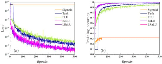
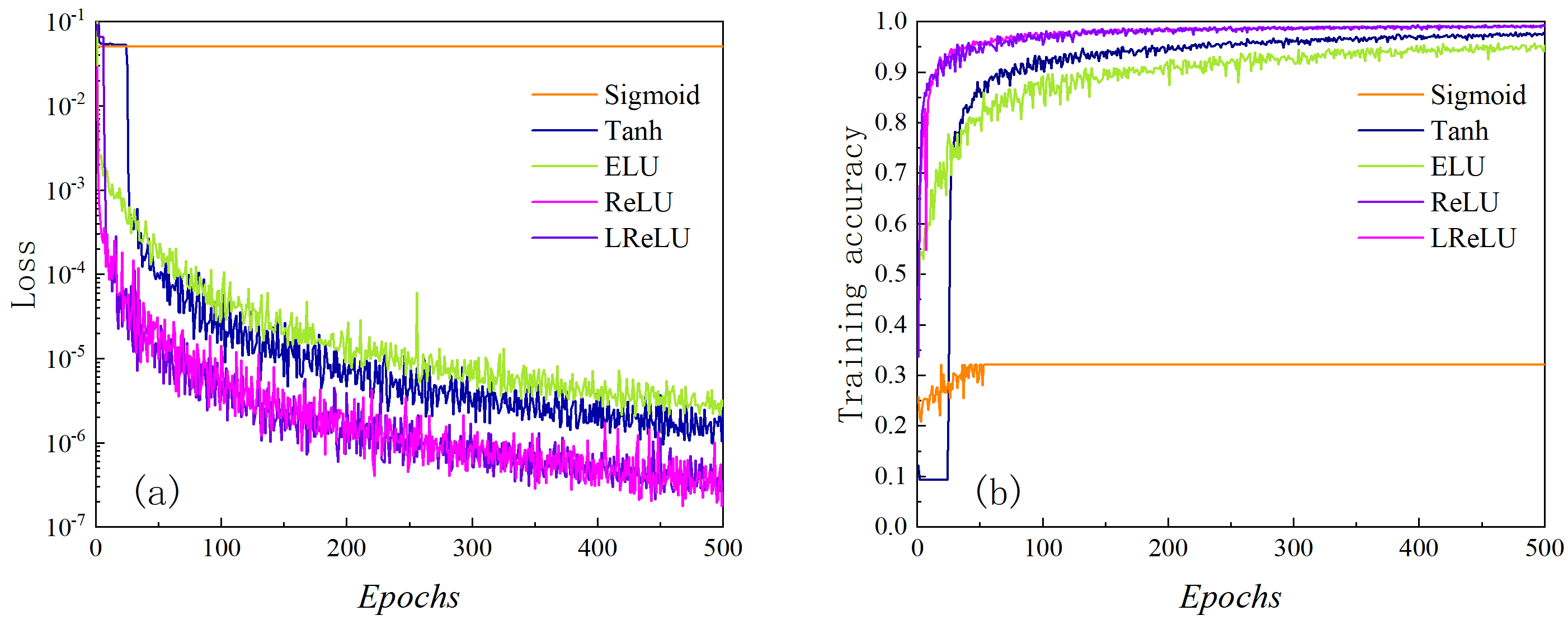
Here, a five-layer network is trained on the dataset using Adam (learning rate = 0.001). The training results for the five activation functions are illustrated in Figure 4, where panel (a) shows the loss function curves and panel (b) shows the training accuracy curves.

Figure 4. Training results generated by five activation functions: (a) loss curve; (b) training accuracy curve.

It can be observed that: (1) ReLU and LReLU perform similarly, both outperforming Tanh, ELU, and Sigmoid in loss reduction and accuracy. Sigmoid, however, tends to fall into local minima and thus exhibits the poorest performance. (2) Given that all resistivity response database entries are normalized to the range [0, 1], the LReLU function cannot handle negative anomalous values if they appear in the input vector of any layer, which would significantly degrade training performance. The ReLU function, by contrast, circumvents this issue. Furthermore, following random network initialization, approximately 50% of neurons in ReLU-activated layers remain inactive. This sparsity prevents neuron saturation, reduces interdependencies between adjacent layers, and improves computational efficiency. Consequently, ReLU is selected as the activation function in this paper.

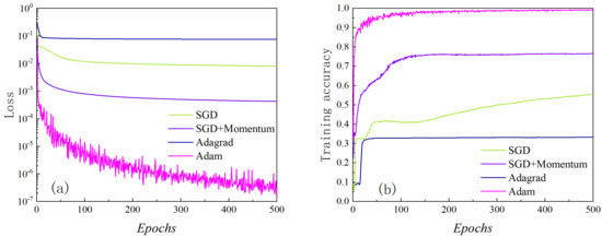
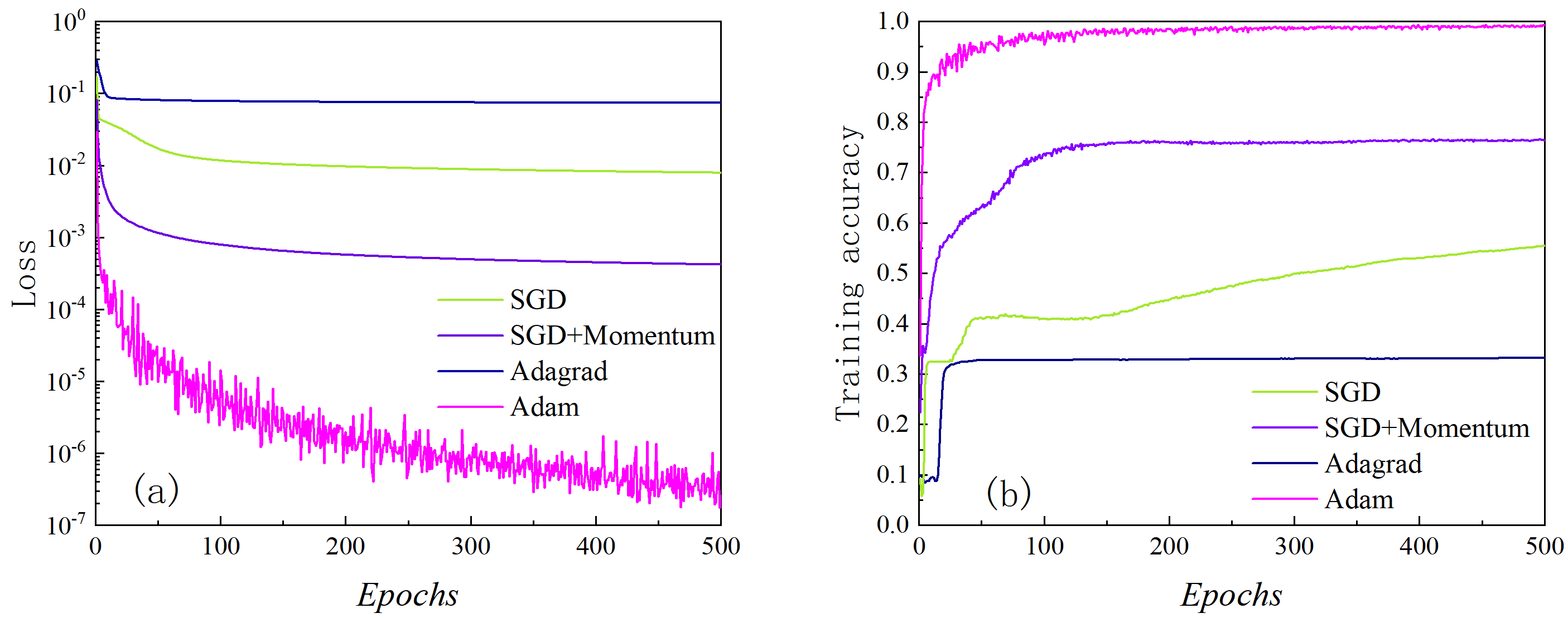
Training algorithms for deep neural networks include Stochastic Gradient Descent (SGD), SGD with momentum (SGD + Momentum), Adagrad, and Adam. Figure 5 compares their training performance, with the same network configuration (layer count and neuron number) as in the previous section and ReLU as the activation function. Adam clearly exhibits superior learning capability relative to Adagrad, SGD + Momentum, and vanilla SGD. Hence, Adam is selected as the optimizer for this study.

Figure 5. Training results generated by four training algorithms: (a) loss curve; (b) training accuracy curve.

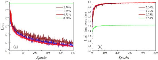
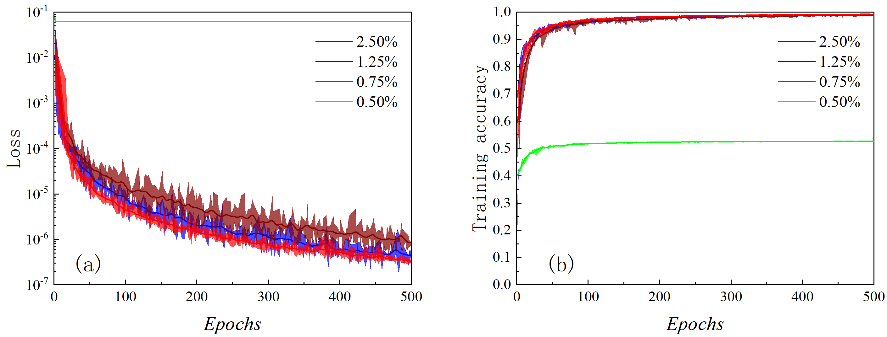
To reduce update variance and improve convergence stability, training data are split into mini-batches. Batch size is the size of each mini-batch. For the deviated/horizontal borehole resistivity dataset, the batch sizes corresponding to 0.5%, 0.75%, 1%, 1.25%, and 2.5% of the full dataset are tested. Figure 6 shows that model performance improves with smaller batch size ratios. Relative to 2.5%, a 1.25% ratio reduces loss by 37.7% and improves accuracy by 3.37%; a 0.75% ratio cuts loss by 61.9% and boosts accuracy by 5.10%. However, reducing the batch size ratio excessively leads to a sharp deterioration in model performance. As shown in the figure, at a ratio of 0.50%, the prediction accuracy drops dramatically and the loss function fails to converge. The reason is that an overly small batch size produces gradient estimates that no longer approximate the global gradient direction of the entire training set. Consequently, the optimization process trapped in a local minimum, preventing any further improvement in network training performance.

Figure 6. Training results generated by four batch sizes: (a) loss curve; (b) training accuracy curve.

Therefore, the optimal batch size for the deviated/horizontal borehole resistivity response database is determined to be 0.75% of the total training set.

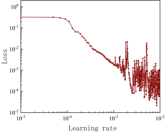
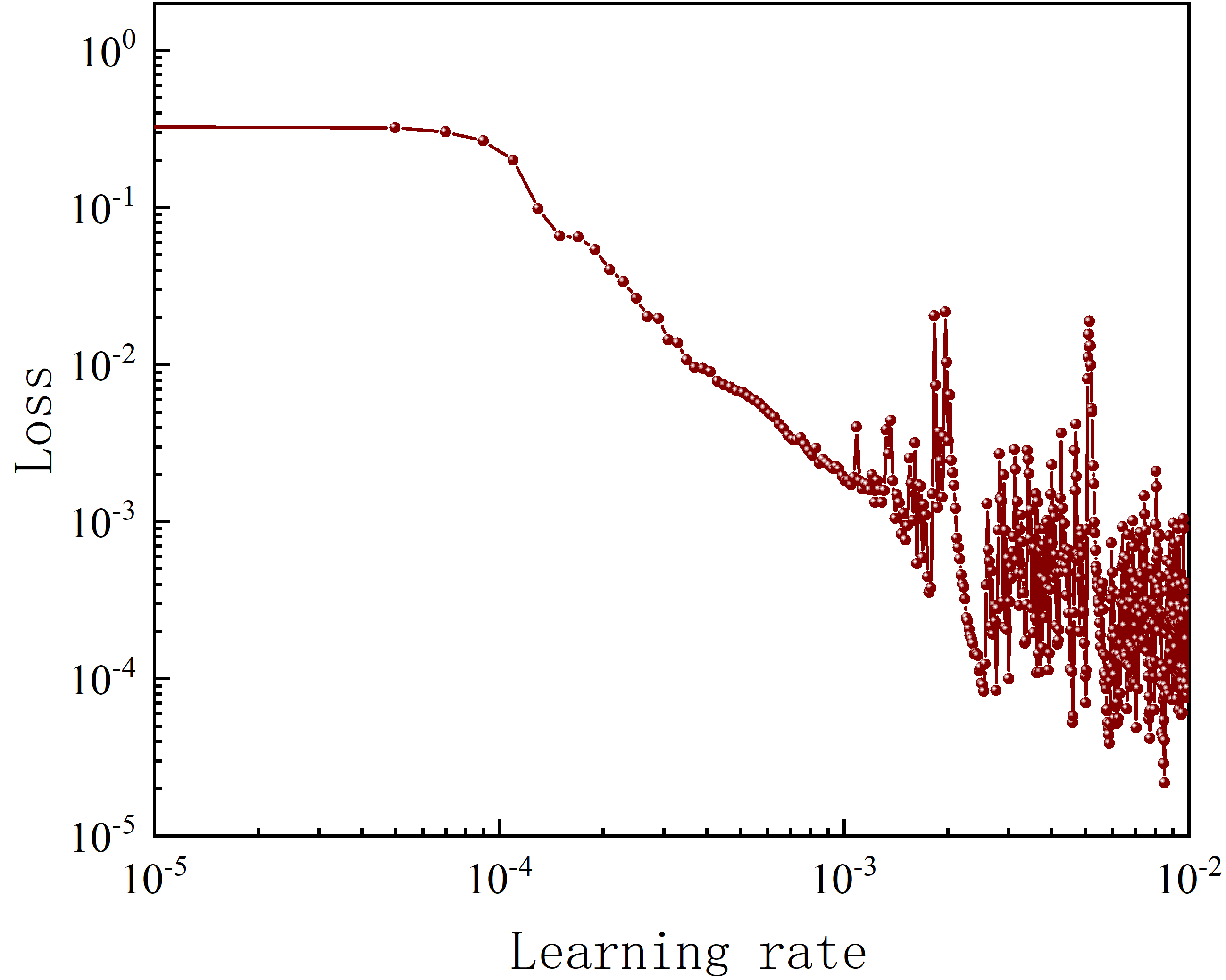
As seen from the training results, deep neural networks suffer from significant oscillations in loss and accuracy during iterations due to their large parameter count and heavy gradient computations. This instability undermines gradient updates and increases prediction uncertainty. The learning rate is the direct stability factor: a too-small rate causes slow convergence, while a too-large rate leads to drastic loss of oscillations. To address this issue, the “variable learning rate” algorithm that adapts the learning rate based on the iteration count is proposed, thereby enabling rapid and adaptive learning rate optimization. The main procedure is outlined as follows:

Step 1. Define the learning rate range as [min_lr, max_lr], where min_lr = 10⁻⁵, max_lr = 10⁻².

Step 2. Based on the iteration number, define the learning rate at each iteration as follows:

$$lr=\min \_lr+{\displaystyle \frac{(\max \_lr-\min \_lr)\ast n}{epochs}}$$

(14)

where epochs is the total number of iterations, here set to 500, and n is the iteration index ranging from 1 to 500.

Step 3. Start training based on the defined neural network framework.

Step 4. After training, extract the learning rate values as a function of the iteration number, along with the corresponding loss function values for each learning rate, and determine the optimal learning rate range.

The curve of the loss function value as a function of the learning rate after training is shown in the figure.

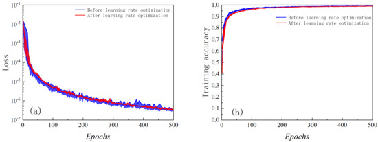
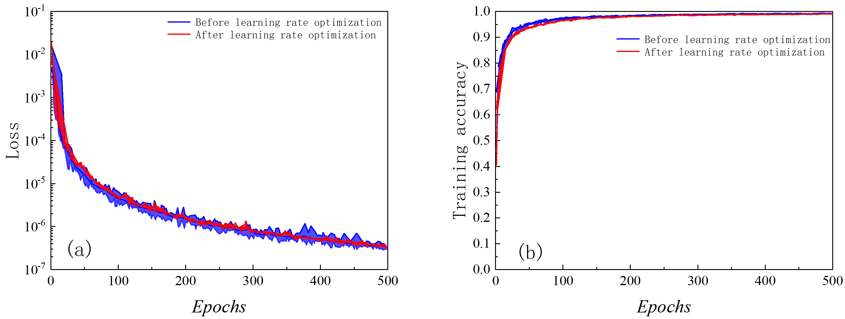
Figure 7 shows that a too-small learning rate traps the loss in a local minimum (no convergence). Raising it to 10⁻⁴ allows Adam to escape local extrema and converge smoothly. Above 0.001, the loss oscillates and training becomes unstable. Thus, the preferred learning rate for our dataset lies between 10⁻⁴ and 10⁻³. Training with this range yields Figure 8 (blue: before optimization, red: after). As can be seen, the oscillations in the training results are greatly suppressed, leading to a marked improvement in neural network model performance.

Figure 7. Loss values generated by different learning rates.

Figure 8. Training results before and after learning rate optimization: (a) loss curve; (b) training accuracy curve.

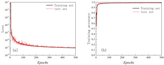
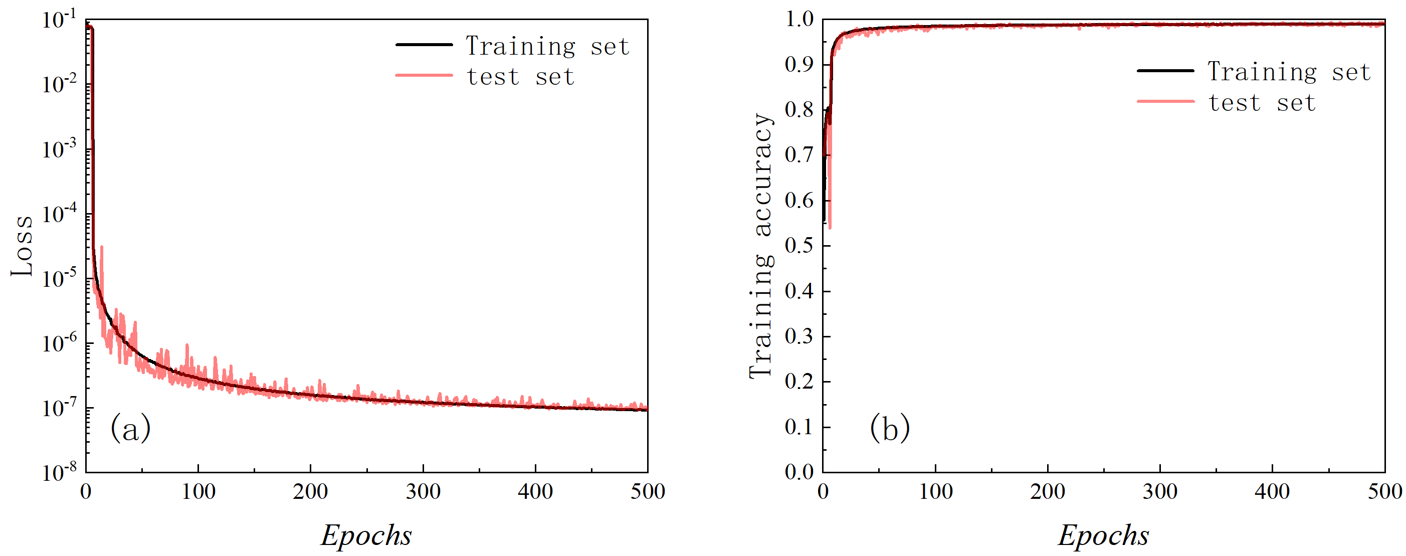
Thus far, the fully connected deep neural network framework adopted in this section has been established. The training scheme proceeds as follows: the resistivity response database is normalized, then randomly divided into a training set (95%) and a test set (5%). A five-layer DL model is trained on the training set using the ReLU activation function, the Adam optimizer, a batch size of 0.75% of the training set, and a learning rate in the range of 10⁻⁴ to 10⁻³.

The neural network architecture established above is employed to train the borehole resistivity response database, and the results are presented in Figure 9. Panels (a) and (b) plot loss and accuracy versus iterations for training and test sets. The following observations can be made: (1) Once the number of iterations exceeds 300, the performance of the fully connected neural network model gradually approaches an optimum, with the loss function converging accordingly. At 500 iterations, the loss function converges to 10⁻⁷, and the prediction accuracy reaches 99.5%. (2) The suitably selected learning rate range prevents significant oscillations in both loss and accuracy, indicating robust model performance. (3) The test set curves for loss and accuracy closely track those of the training set. (4) Because the test set and training set are randomly selected without overlap, the test set prediction accuracy of 99.3% demonstrates the strong generalization capability of the trained model. Consequently, this network can effectively and accurately compute borehole resistivity response data.

Figure 9. Training results for borehole resistivity dataset: (a) loss curve; (b) training accuracy curve.

2.2. Modeling Accuracy Analysis

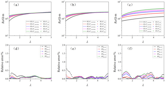
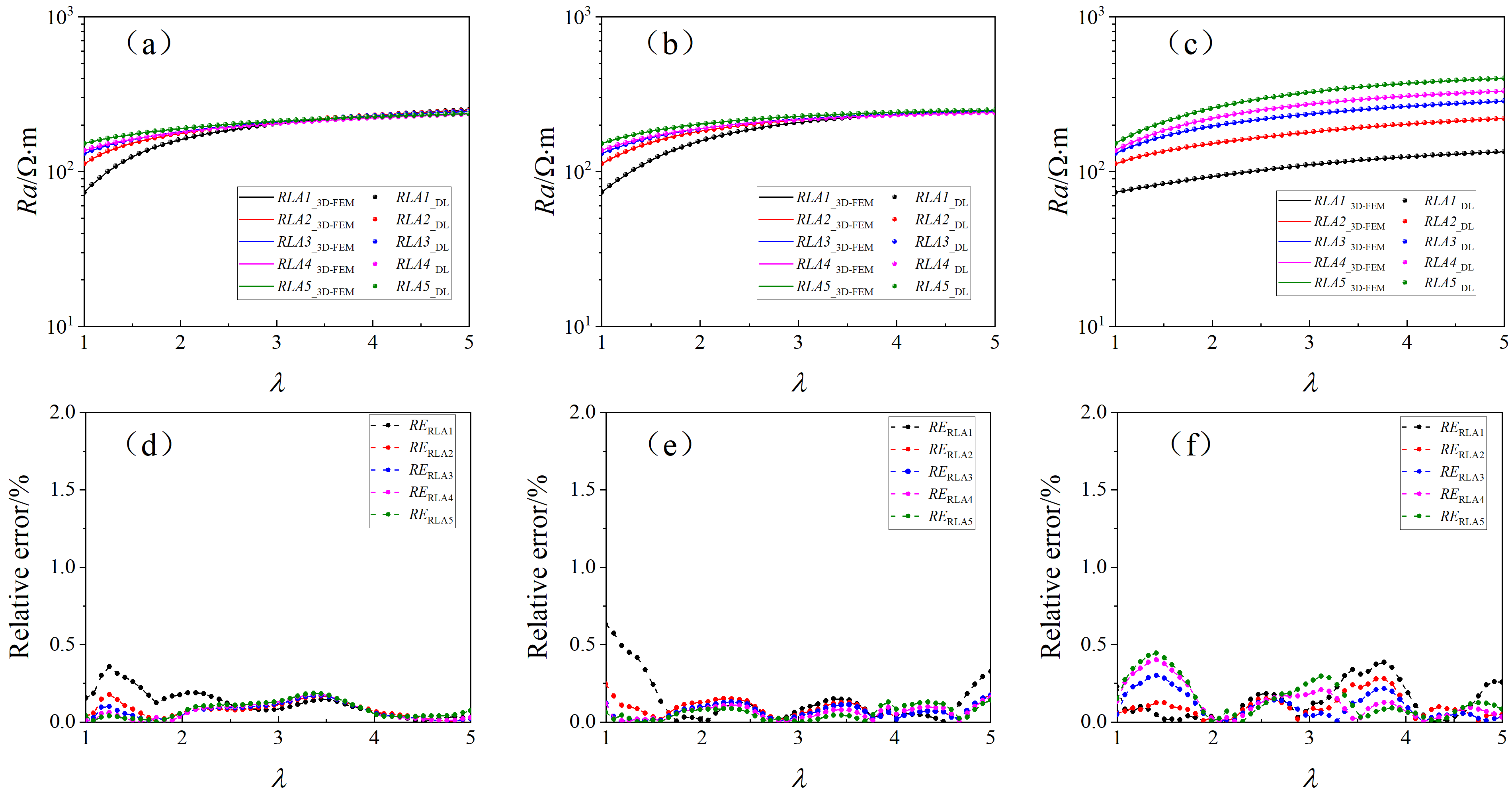
To further assess the stability and reliability of the DL-based forward model, this section compares its predicted results with those obtained from rigorous 3D-FEM simulations. The formation model is defined as follows: deviation angles of 0°, 30°, and 80°; borehole diameter of 8 in.; mud resistivity of 0.1 Ω·m; invasion depth of 0.3 m; invaded-zone horizontal resistivity of 20 Ω·m; resistivity contrast of 10; and anisotropy coefficient ranging from 1 to 5. Figure 10a–c present the predicted apparent resistivity (Ra) for the three deviation angles alongside the corresponding 3D-FEM simulation results, and Figure 10d–f show the respective relative error curves. It can be observed that the apparent resistivity curves predicted by the model are in good agreement with those from the simulations; both sets of curves increase progressively with the anisotropy coefficient. The relative error curves indicate a strong match between the model predictions and finite element results, with a maximum relative error of 0.61%.

Figure 10. Effect of anisotropy coefficient on prediction accuracy: (a) Ra (θ = 0°); (b) Ra (θ = 30°); (c) Ra (θ = 80°); (d) Relative error (θ = 0°); (e) Relative error (θ = 30°); (f) Relative error (θ = 80°).

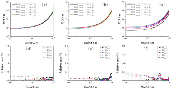
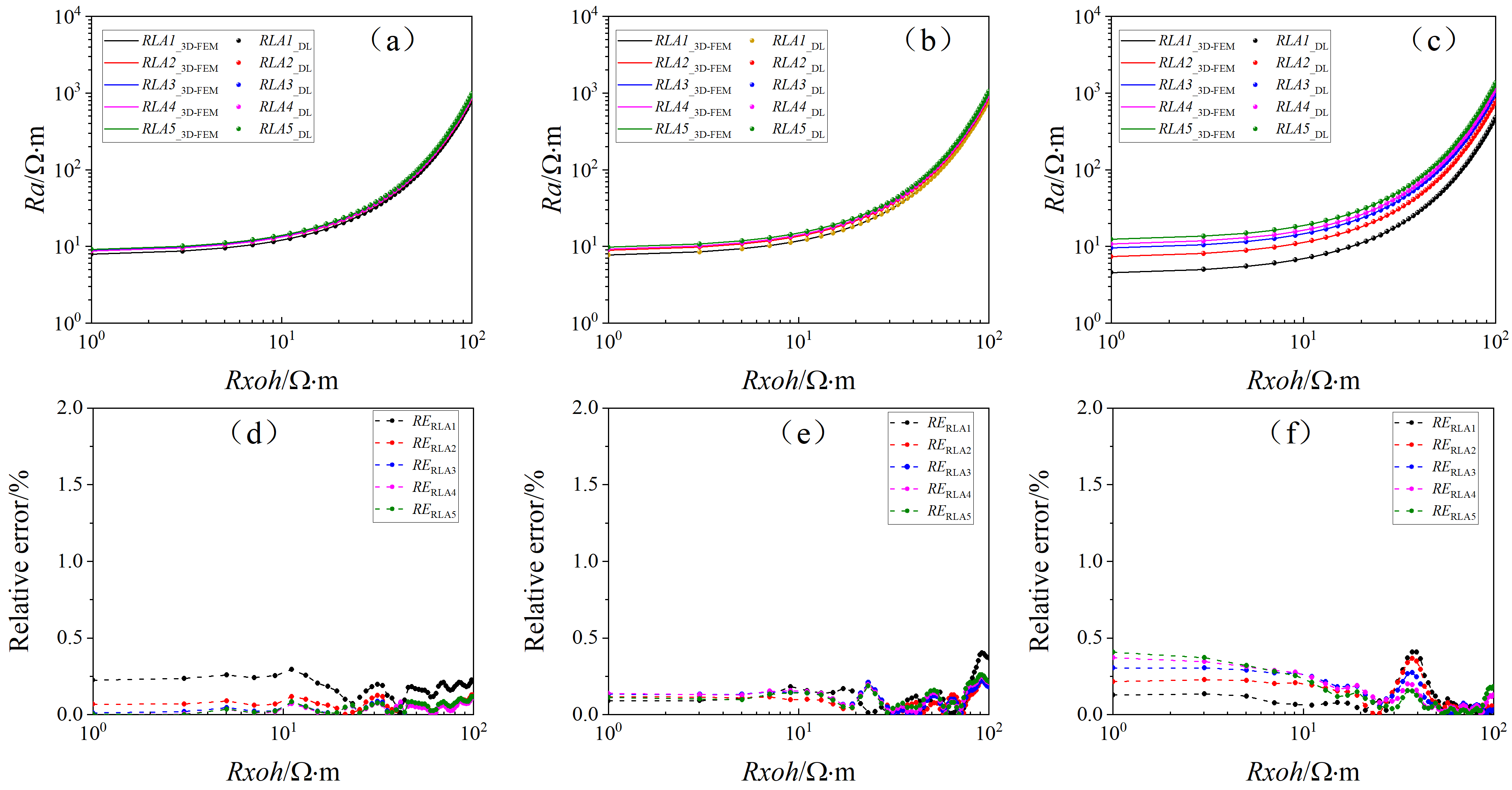
The effect of invaded-zone horizontal resistivity on the model’s prediction accuracy is evaluated. The formation model is defined with deviation angles of 0°, 30°, and 80°; borehole diameter of 8 inches; mud resistivity of 0.1 Ω·m; invasion depth of 0.3 m; invaded-zone horizontal resistivity ranging from 1 to 100 Ω·m; anisotropy coefficient of 2; and resistivity contrast of 10. Figure 11a–c present the predicted results alongside the 3D finite element simulation results for the three deviation angles, and Figure 11d–f give the corresponding relative error curves. The results demonstrate that the apparent resistivity curves increasing with the horizontal resistivity of the invaded zone. Furthermore, larger deviation angles amplify the influence on the five apparent resistivity curves, leading to greater separation among them. The relative error curves confirm excellent agreement between the two simulation outcomes, with a maximum relative error of 0.49% under the given formation model.

Figure 11. Effect of invaded horizontal resistivity on prediction accuracy: (a) Ra (θ = 0°); (b) Ra (θ = 30°); (c) Ra (θ = 80°); (d) Relative error (θ = 0°); (e) Relative error (θ = 30°); (f) Relative error (θ = 80°).

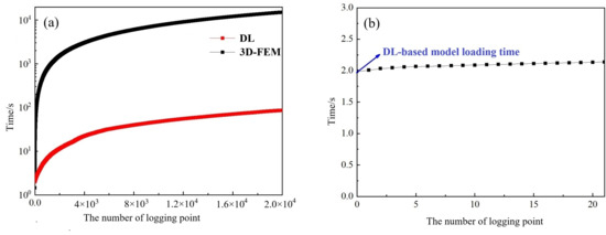
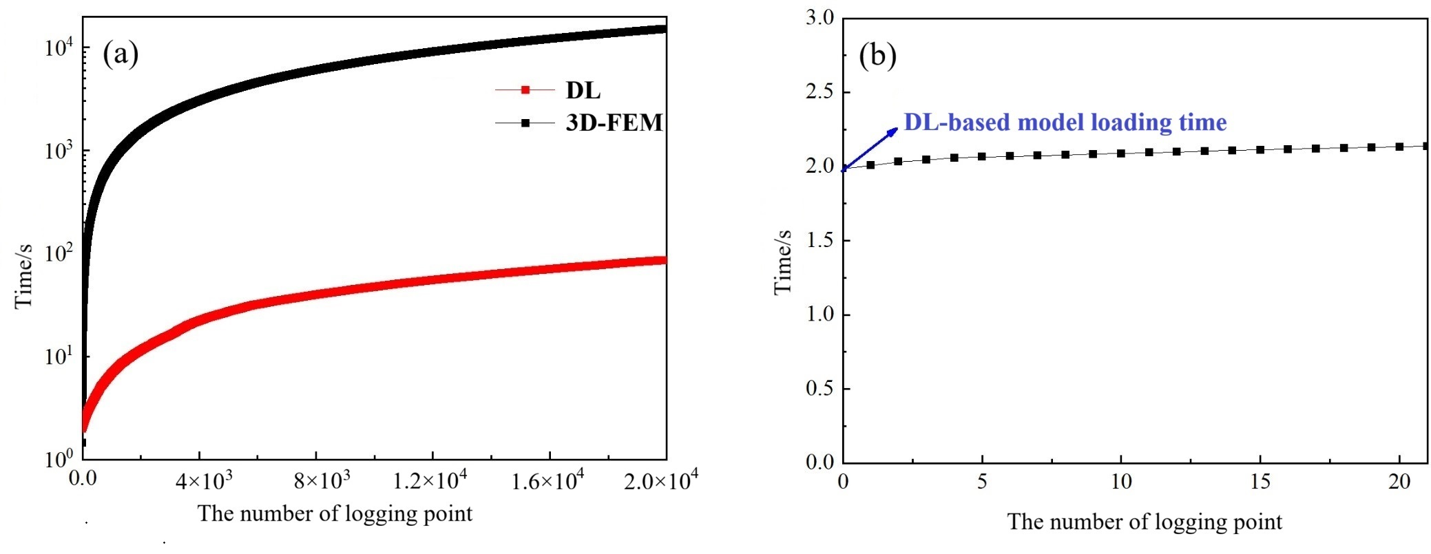
The most significant advantage of the DL model is its dramatically improved forward modeling efficiency, as illustrated in Figure 12a. The horizontal axis denotes the number of logging points, and the vertical axis the computational time for borehole resistivity responses. The DL model requires only about 0.0042 s per logging point, compared to approximately 0.68 s for the 3D finite element method. Thus, the DL achieves a speedup factor of roughly 162 s for a single logging point. This efficiency gain becomes even more pronounced as the number of logging points increases. For instance, computing 20,000 logging points takes the DL 86 s (0.024 h), whereas 3D-FEM requires 15,051 s (4.181 h).

Figure 12. Computational efficiency comparison: (a) Time consumption of the two models (3D-FEM vs. DL) for different numbers of logging points; (b) DL model loading time.

It is also worth noting that loading the DL model before invoking it incurs a certain time overhead, as shown in Figure 12b. The first data point in the figure corresponds to this model loading time, which is approximately 1.97 s.

3. Adaptive Regularized Inversion Algorithm

The Levenberg–Marquardt (LM) algorithm, despite combining steepest descent and Gauss–Newton advantages, cannot ensure global convergence for strongly nonlinear inversion problems. Its inherent second-order convergence also leads to slow processing, inadequate for real-time evaluation. To address these issues, a modified LM algorithm with third-order convergence is presented, achieved via an improved step-size scheme that boosts global optimization.

Typically, the parameter iteration formula of the LM algorithm is as follows [38,39]

$$y_k=x_{k-1}+d_k$$

(15)

where k is the current iteration number, $d_k=-J_k^T\cdot C\left(x_k\right)\cdot {\left(J_k^T{J}^k+{\mu }_k\mathit{I}\right)}^{-1}$.

The adaptively modified LM (AMLM) algorithm then refines the update direction based on the previous iteration, yielding the new iteration formula [40]:

$$d_{1k}=-J_k^T\cdot C\left(y_k\right)\cdot {\left(J_k^T{J}^k+{\mu }_k\mathit{I}\right)}^{-1}$$

(16)

$$x_k=y_k+{\alpha }_k\cdot d_{1k}$$

(17)

where ${\alpha }_k$ is the iteration step size in the direction of $d_{1k}$, which is typically determined using a line search method:

$$\underset{{\alpha }_k>0}{\min }‖C\left(y_k+{\alpha }_k{d}_{1k}\right)‖$$

(18)

According to Taylor expansion, the above equation is equivalent to the following:

$$\underset{{\alpha }_k>0}{\max }\Phi \left({\alpha }_k\right)={\displaystyle \sum _{i=1}^m{‖f_i\left(y_k\right)‖}^2-{‖f_i\left(y_k\right)+{\alpha }_k{J}_k{d}_{1k}‖}^2}$$

(19)

Therefore,

$${\alpha }_k=1+{\displaystyle \frac{{\mu }_k{d}_{1k}^T{d}_{1k}}{d_{1k}^T{J}_k^T{J}_k{d}_{1k}}}$$

(20)

Because when $J_k{d}_{1k}$ is large enough, ${\alpha }_k$ approaches 0, to avoid losing the iteration information from the previous step, we define:

$${\alpha }_k=\min \left\{{\alpha }_k,\widehat{\alpha }\right\}$$

(21)

where $\widehat{\alpha }>1$.

Yamashita and Fukushima proved that the LM algorithm achieves second-order convergence even when ${\mu }_k=‖C_k‖$ [41]. Fan et al. subsequently modified it to ${\mu }_k={\zeta }_k{‖C_k‖}^{{\displaystyle \raisebox{1ex}{$\delta $}\!\left/ \!\raisebox{-1ex}{$2$}\right.}}$ and demonstrated that the convergence order is governed by E, but never exceeds three [42].

Keyvan et al. further proposed a hyperparameter update method (shown below) that ensures stable third-order convergence of the AMLM algorithm without sacrificing accuracy.

$${\delta }_k=\left\{\begin{array}{l}{\displaystyle \frac{1}{{‖C_k‖}^{\raisebox{1ex}{$1$}\!\left/ \!\raisebox{-1ex}{$2$}\right.}}}\begin{array}{cc} & \end{array}if{‖C_k‖}^{{\displaystyle \raisebox{1ex}{$1$}\!\left/ \!\raisebox{-1ex}{$2$}\right.}}\\ 1+{\displaystyle \frac{1}{k}}\begin{array}{cc} & \end{array}otherwise\end{array}\right.$$

(22)

$${\mu }_k={\zeta }_k{‖C_k‖}^{{\displaystyle \raisebox{1ex}{${\delta }_k$}\!\left/ \!\raisebox{-1ex}{$2$}\right.}}$$

(23)

The update procedure for the ${\zeta }_k$ is as follows

$${\zeta }_k=\left\{\begin{array}{c}4{\zeta }_k\\ {\zeta }_k\\ \max \left({\zeta }_k/4,m\right)\end{array}\begin{array}{c}if\left(r_k<p_1\right)\\ if\left(r_k\in \left[p_1,p_2\right]\right)\\ otherwise\end{array}\right.$$

(24)

where P₁, P₂, and m are typically positive numbers less than 1.

The evaluation function is:

$$r_k={\displaystyle \frac{‖C\left(x_k\right)‖-‖C\left(x_k+d_k+{\alpha }_k\cdot d_{1k}\right)‖}{‖C\left(x_k\right)‖-‖C\left(x_k\right)+J\left(x_k\right)d_k‖+‖C\left(y_k\right)‖-‖C\left(y_k\right)+{\alpha }_{k}J\left(x_k\right)d_{1k}‖}}$$

(25)

where $y_k=x_k+d_k$.

The adaptive damping parameter μ is updated according to the gain ratio r_k, which measures the actual reduction in the misfit against the predicted reduction. This strategy ensures fast third-order convergence while maintaining stability. It can be observed that during each parameter update, C(x_k), J(x_k), and d_k are already available from the standard LM algorithm. The only extra computation is d_1k. Thus, the AMLM algorithm achieves third-order convergence at the cost of only one additional forward modeling per iteration.

4. Synthetic Data Examples

4.1. High-Resistivity Anisotropic Formation

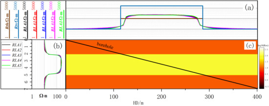
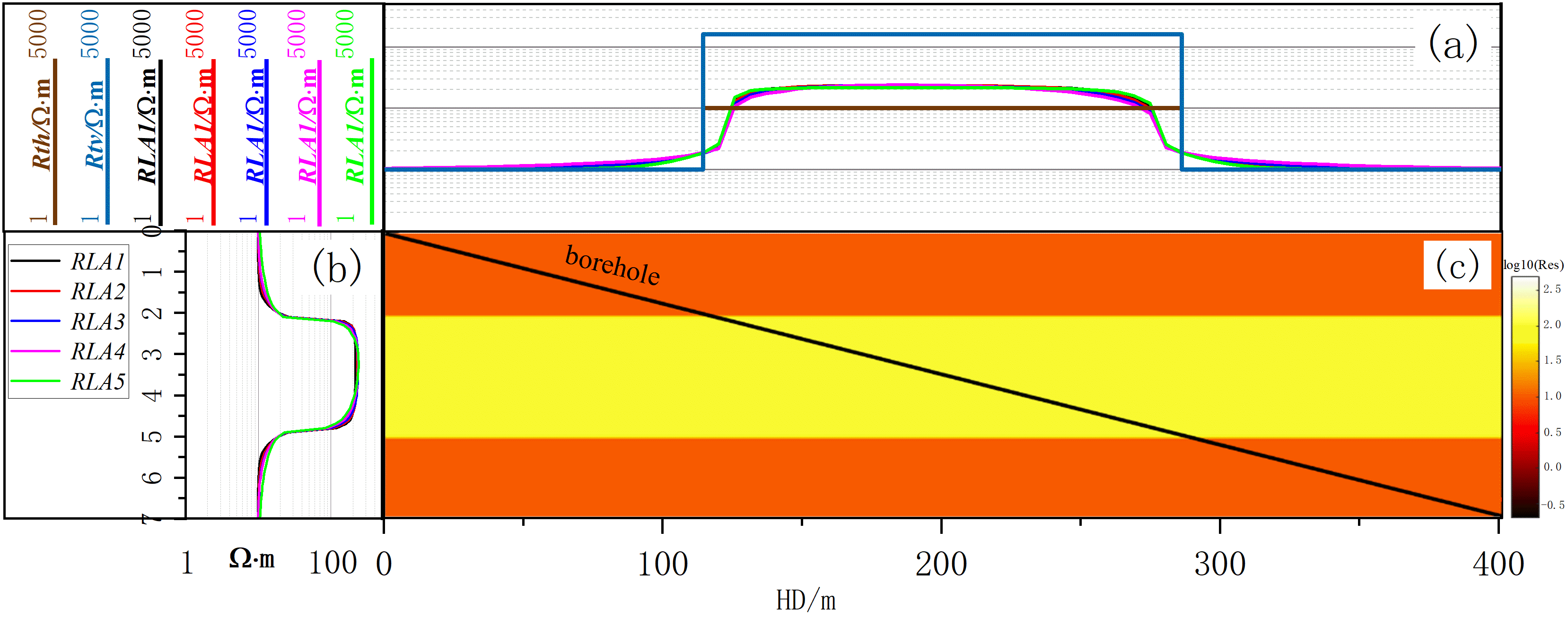
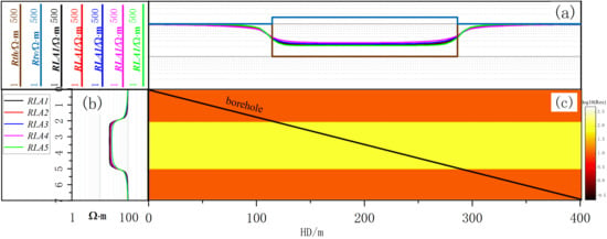
To validate the effectiveness of the fast inversion method, a three-layer horizontal interface model is constructed in this section. The borehole diameter is 8 inches, and the mud resistivity is 0.1 Ω·m. The middle layer is an anisotropic high-resistivity formation with a horizontal resistivity of 100 Ω·m and an anisotropy coefficient of 4. The first and third layers are isotropic formations with a resistivity of 10 Ω·m, as illustrated in Figure 13c, where the black solid line indicates the well trajectory with a deviation angle of 89°. Figure 13b shows the apparent resistivity logs of the corresponding pilot well for this formation model, and Figure 13a presents the horizontal apparent resistivity information. The initial bed boundary locations and formation resistivity values can be obtained by processing the pilot well data, which can then be used as prior information to constrain the inversion process.

Figure 13. Formation model with well trajectory: (a) horizontal and vertical resistivities, borehole resistivity responses; (b) apparent resistivity curves from pilot well; (c) formation model.

The logging responses in the figure show that the apparent resistivity in the target zone is severely affected by anisotropy. The measured values are approximately twice the true formation resistivity, thus failing to represent the actual formation resistivity. Hence, inversion is necessary to reconstruct the true resistivity profile.

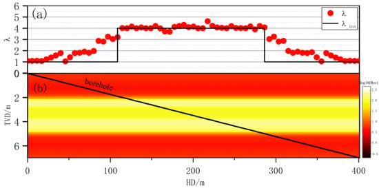
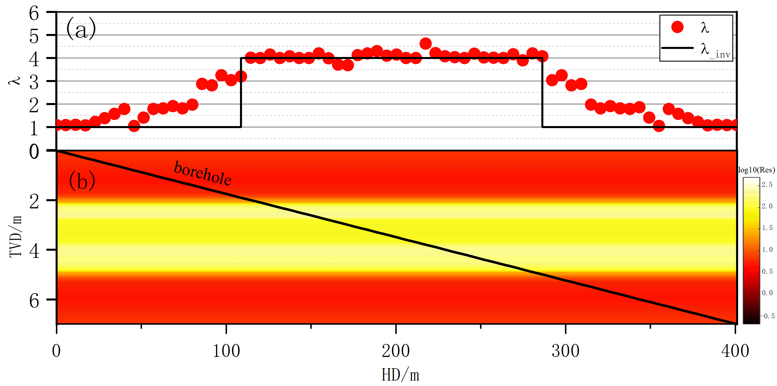
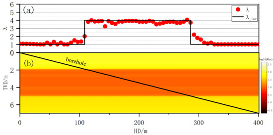
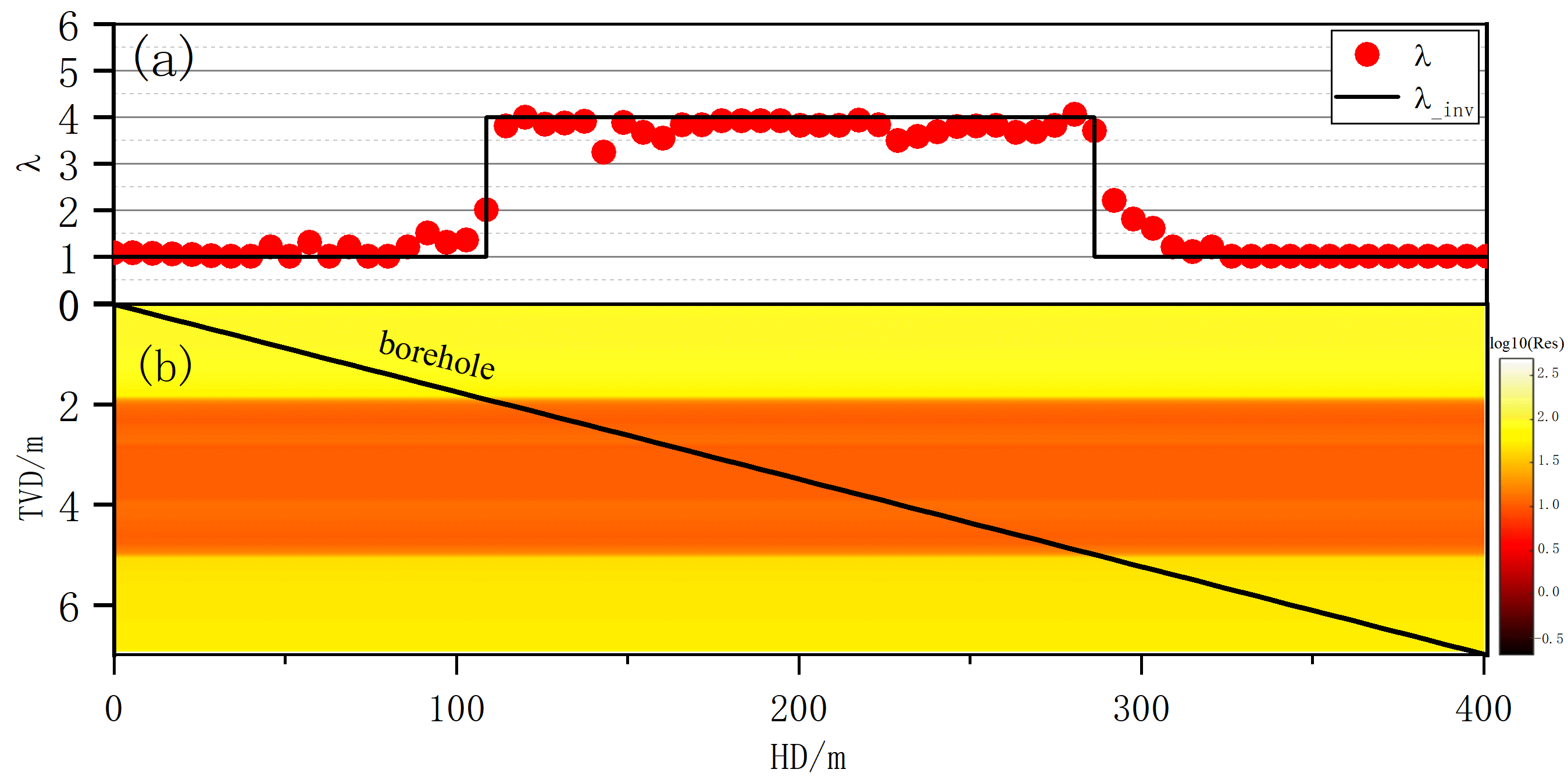
Figure 14a shows the inverted anisotropy coefficient in the target zone (black line: true values while drilling; red dots: inverted results). Figure 14b presents the 2D horizontal resistivity image, with brighter colors indicating higher resistivity. The average per-point relative errors (the mean of relative errors over all logging points) for horizontal resistivity and anisotropy coefficient are 6.82% and 6.97%, respectively, demonstrating the accuracy and reliability of the proposed fast horizontal-well resistivity imaging method.

Figure 14. Inversion results: (a) anistropic coefficients; (b) 2-D resistivity image.

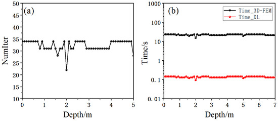
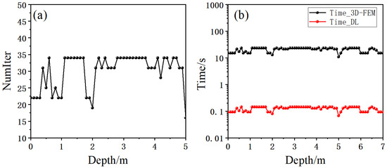
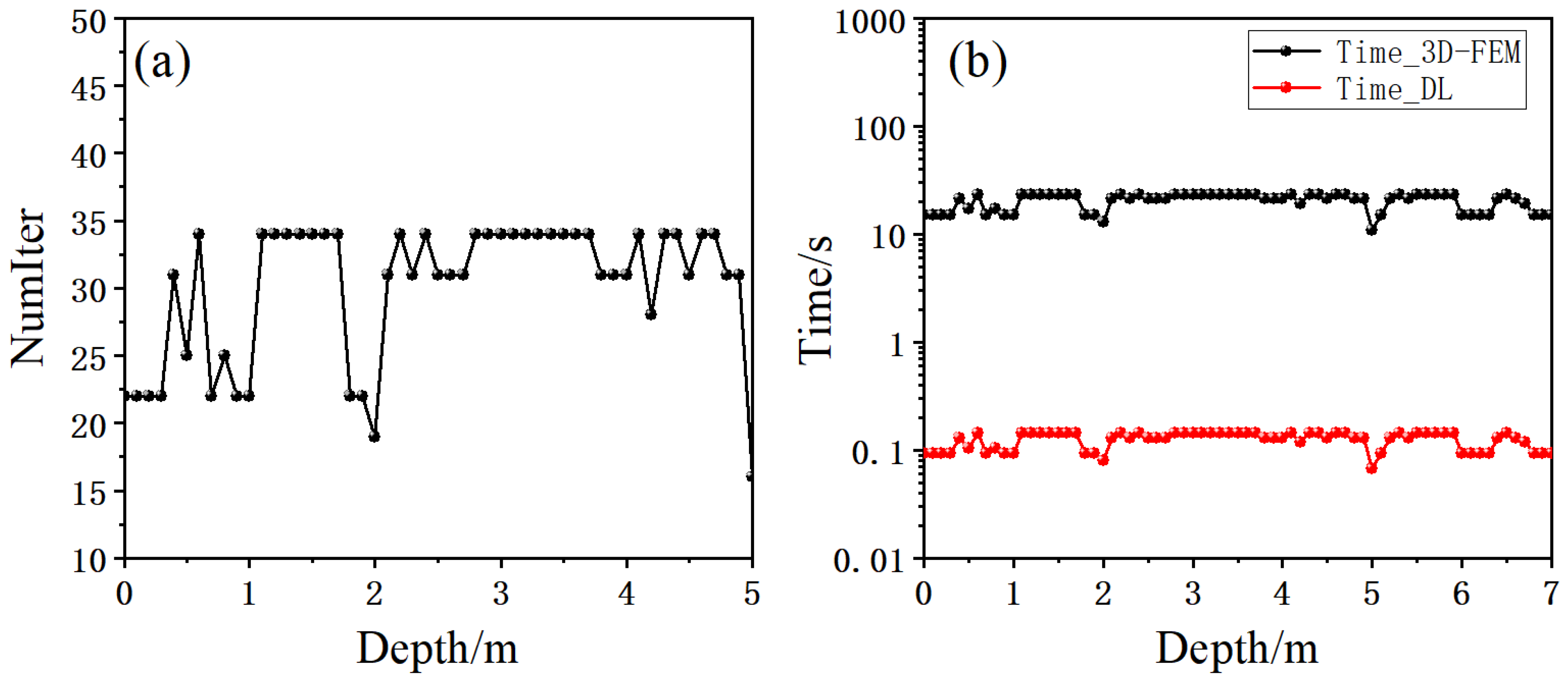
Figure 15 shows the number of forward modeling calls required for convergence at each logging point for this model. The right panel presents the time per logging point upon convergence, where the black and red bars correspond to the 3D FEM and the fast forward model, respectively. The fast forward model takes only about 0.15 s per logging point, whereas 3D FEM requires more than 11 s. The total time across all logging points is 10.65 s for the fast model versus 781 s for 3D FEM, yielding an efficiency improvement of 98.64%.

Figure 15. Convergence performance: (a) number of forward modeling calls; (b) time consumption.

4.2. Low-Resistivity Anisotropic Formation

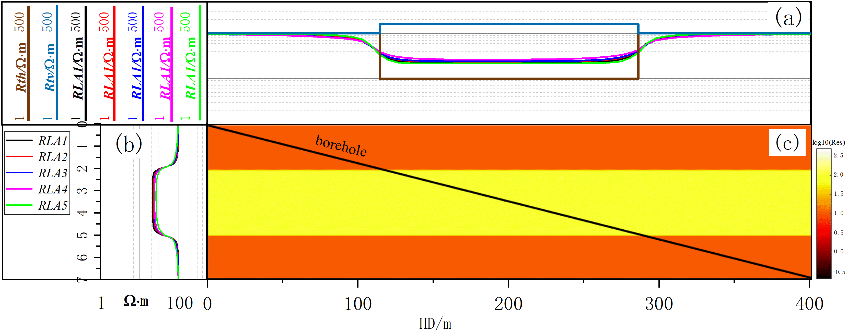
To further evaluate the performance of the algorithm in a low-resistivity interlayer model, a three-layer horizontal interface model is constructed. The borehole diameter is 8 inches, and the mud resistivity is 0.1 Ω·m. The middle layer is an anisotropic low-resistivity formation with a horizontal resistivity of 10 Ω·m and an anisotropy coefficient of 4. The first and third layers are isotropic formations with resistivities of 100 Ω·m and 50 Ω·m, respectively, as illustrated in Figure 16a,c, where the black solid line indicates the well trajectory with a deviation angle of 89°. As can be seen from the logging responses in the figure, the apparent resistivity in the target zone is still severely affected by anisotropy, with measured values exceeding the true formation resistivity.

Figure 16. Formation model with well trajectory: (a) horizontal and vertical resistivities, borehole resistivity responses; (b) apparent resistivity curves from pilot well; (c) formation model.

Figure 17 shows the inversion results. Average relative errors per logging point are 6.82% (horizontal resistivity) and 6.97% (anisotropy coefficient). Inversion accuracy is higher in the low-resistivity interlayer than in the high-resistivity case, because the low-resistivity medium enhances current propagation, enabling apparent resistivity responses to carry more formation information. These results further validate the proposed fast resistivity imaging method for horizontal wells.

Figure 17. Inversion results: (a) anistropic coefficients; (b) 2-D resistivity image.

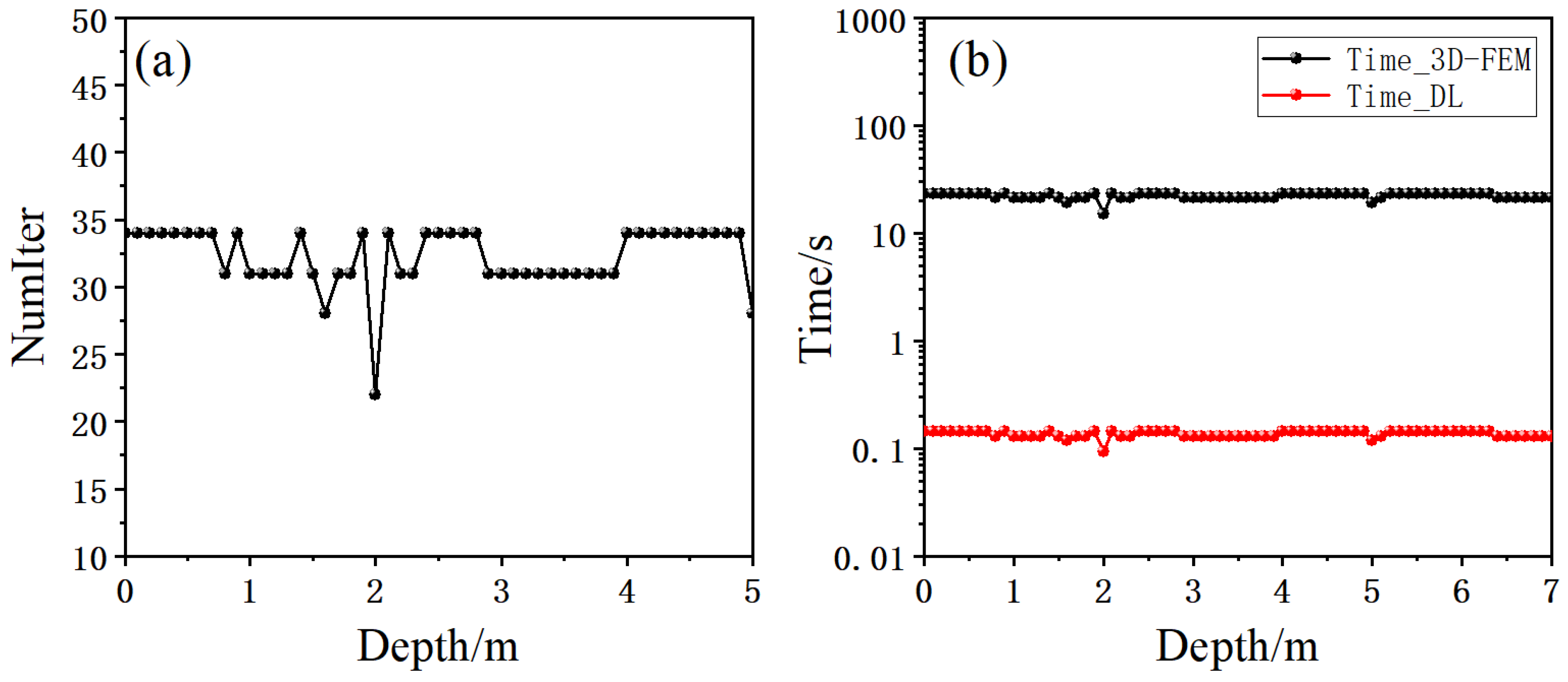
Similar to Figure 15, Figure 18 shows the number of forward modeling calls (left) and the time per logging point (right) required for inversion convergence. The black and red bars denote the 3D FEM and the fast forward model, respectively. The fast model takes only about 0.15 s per logging point, whereas 3D FEM requires more than 11 s. The total computation time for all logging points is 10.65 s using the fast model, compared to 781 s using 3D FEM, yielding an efficiency improvement of 98.64%.

Figure 18. Convergence performance: (a) number of forward modeling calls; (b) time consumption.

4.3. Multi-Layer Anisotropic Formation

During logging, resistivity tools often traverse multiple layer boundaries, acquiring information from several formations. In this section, a multi-layer model is constructed to investigate the effect of layer boundaries on inversion results.

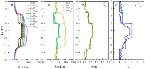
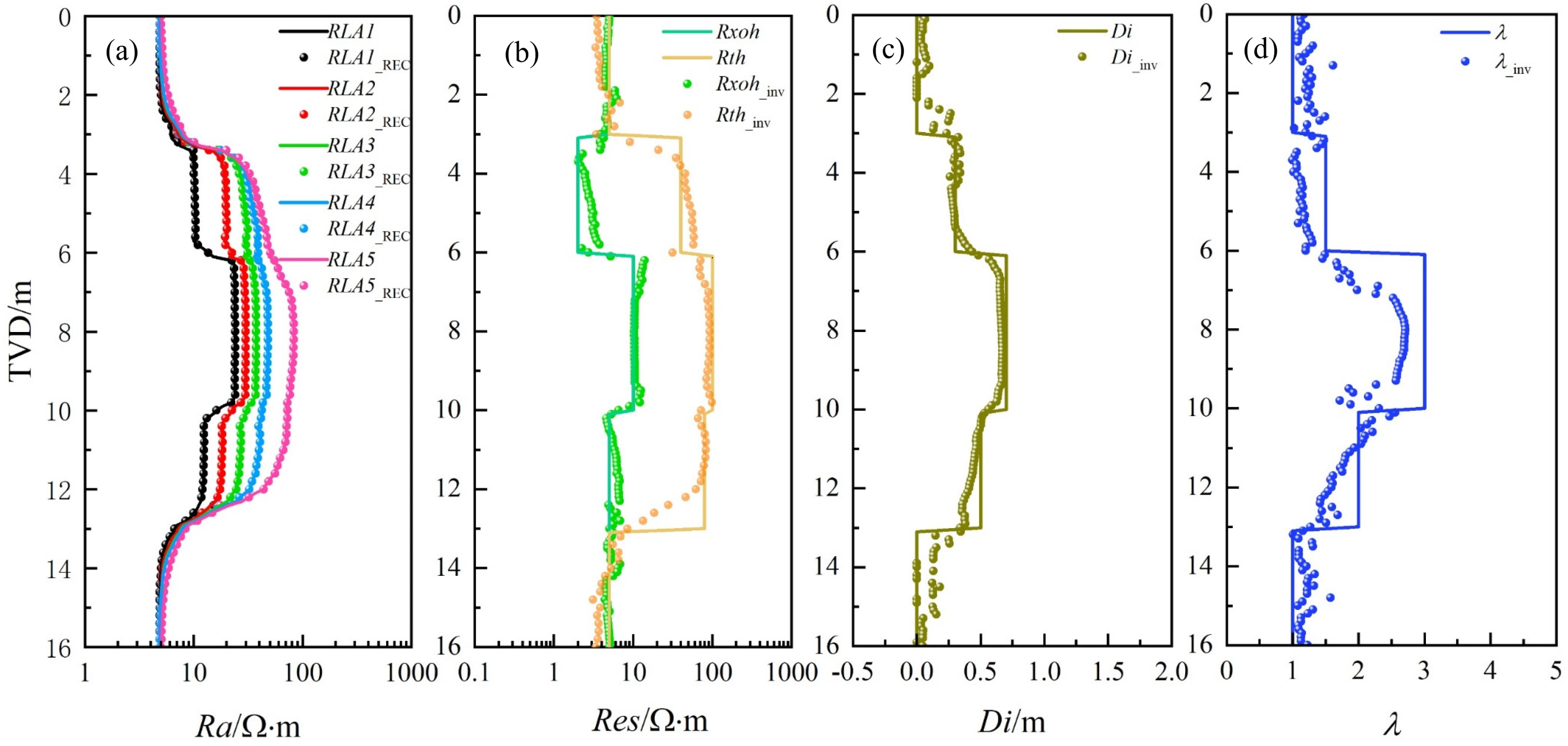
A five-layer formation model with a deviation angle of 30° is established. The parameters for each layer, namely layer thickness, invasion depth, and anisotropy coefficient, are summarized in Table 3. Figure 19 illustrates the inverted parameter distribution. The borehole resistivity responses and the inversion-reconstructed curves are shown in Figure 19a. Figure 19b–d present a comparison between the inverted results and the true model values for invaded-zone resistivity, undisturbed formation resistivity, invasion depth, and anisotropy coefficient, respectively.

Table 3. Model parameter distribution.

No.	H/m	Di/m	Rxoh/Ω·m	Rth/Ω·m	λ
①	3	0	5	5	1
②	3	0.3	2	40	1.5
③	4	0.7	10	100	3
④	3	0.5	5	80	2
⑤	3	0	5	5	1

Figure 19. Inversion results: (a) borehole resistivity responses; (b) inverted resistivity; (c) inverted invasion depth; (d) anisotropy coefficient.

The following observations can be made from the inversion results: (1) The original borehole resistivity responses and the reconstructed responses (RLA1_{_REC}~RLA1_{_REC}) are in good agreement, with an average relative error of less than 10% per logging point over the entire interval. (2) Overall, the inversion results effectively capture the vertical and lateral resistivity distribution of the formation, and the estimated true horizontal resistivity meets practical accuracy requirements. (3) Compared with invasion depth and horizontal resistivity, the anisotropy coefficient exhibits lower inversion accuracy, mainly because under low deviation angles, the invasion effect and the true formation resistivity dominate the logging responses. (4) In intervals with mud invasion, the five apparent resistivity curves show significant separation, providing rich invasion-related information that facilitates stable inversion. (5) The point-by-point inversion strategy does not fully account for surrounding bed effects, leading to reduced inversion accuracy near layer boundaries.

In terms of inversion efficiency, this interval contains 161 logging points. The fast computation model takes approximately 21.68 s, whereas the traditional algorithm requires 3510.2 s, clearly demonstrating a significant efficiency improvement.

5. Field Data Example

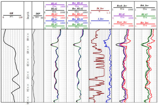
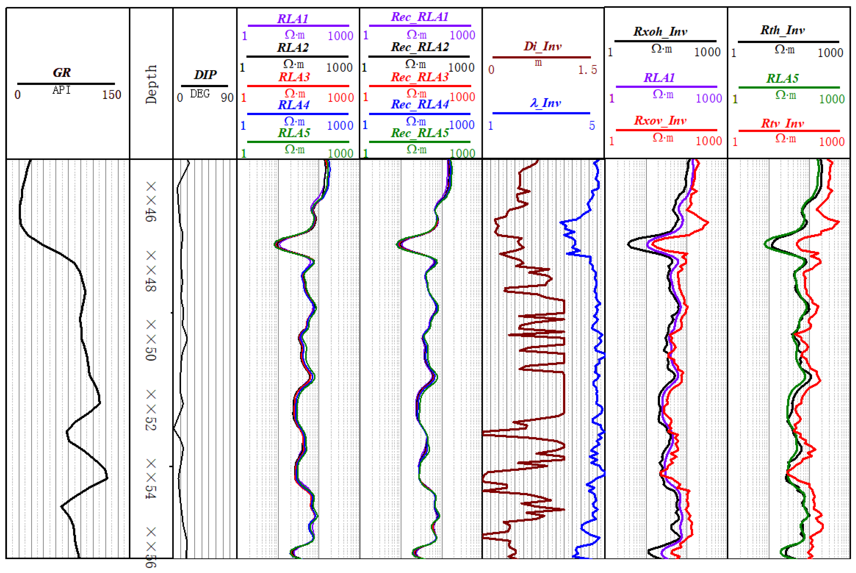
The proposed inversion algorithm was applied to field data from Well X in central-western China, and the results are shown in Figure 20. The logged interval spans from ××46 m to ××56 m. Track 1 presents the natural gamma ray log. Track 2 is the depth track. Track 3 shows the relative formation dip. Track 4 displays the measured apparent resistivity curves. Track 5 presents the apparent resistivity curves reconstructed from the inversion results. Track 6 shows the average relative error between the reconstructed and measured curves. Track 7 presents the inverted invasion depth and formation anisotropy coefficient. Track 8 shows the inverted horizontal and vertical resistivities of the invaded zone along with the shallow-reading apparent resistivity curve RLA1. Track 9 presents the inverted horizontal and vertical resistivities of the undisturbed formation together with the deep-reading apparent resistivity curve RLA5.

Figure 20. Inversion results of field data.

The following observations can be found: (1) As seen in Track 8, the measured RLA1 values lie between the inverted horizontal and vertical resistivities of the invaded zone. This is primarily because, in low-angle formations, the shallow-reading resistivity response is strongly affected by anisotropy, causing the measured RLA1 to exceed Rxo. Thus, the inversion results behave as expected. (2) At low dip angles, the deep-reading curves (e.g., RLA5) are less influenced by anisotropy and are mainly sensitive to low-resistivity invasion, leading to measured RLA5 values that are generally smaller than Rt. A comparison shows that the inversion results are consistent with theoretical expectations. (3) A comparison between the reconstructed apparent resistivity curves and the actual measured curves reveals a good match, with an average relative error of less than 10%, indirectly demonstrating the reliability of the inversion results.

6. Conclusions

This paper presents a fast inversion method for borehole resistivity logging data in deviated/horizontal wells through anisotropic formations, based on a deep neural network forward surrogate and an adaptively modified Levenberg–Marquardt algorithm.

A high-coverage 3D resistivity response database (504,000 samples) was constructed using 3D finite-element forward modeling, covering deviation angle, mud invasion, and anisotropy. The deep neural network (ADNN) was systematically optimized to achieve a single-point forward computation time of 0.0042 s—about 162 times faster than 3D FEM—with a maximum relative error of 0.61%. Numerical inversions show an efficiency improvement of approximately 98 over conventional point-by-point inversion, with average relative errors of 6.82% (horizontal resistivity) and 6.97% (anisotropy coefficient). Application to field data demonstrates that the reconstructed apparent resistivity curves match the measured curves with an average relative error of less than 10%. The inverted invaded-zone resistivities, undisturbed formation resistivities, and anisotropy coefficients are consistent with theoretical expectations, confirming the practical applicability and reliability of the proposed method.

It should be noted that the proposed fast forward model is feasible within the resistivity response database parameter ranges, which cover most practical scenarios. For more complex reservoirs (e.g., carbonates with fractures or wider anisotropy ranges), users can expand the database accordingly and fine-tune the optimization workflow as described in this paper. Furthermore, future work will investigate the influence of in situ stress on anisotropic resistivity by incorporating stress-dependent rock physics models, which will further enhance the applicability of the method.

References

- Jia, C.Z.; Wang, Z.G.; Jiang, L.; Zhao, W. Progress and key scientific and technological problems of shale oil exploration and development in China. World Petroleum Industry 2024, 31, 4. [Google Scholar]
- Zhou, Y.; Xiao, Z.; Li, Y.; Lu, J.; Jiang, Q.; Zhou, X.; Cai, Z.; Wang, X. Lithofacies assemblages of shale and dense shell limestone: Implications for shale oil exploration. Front. Earth Sci. 2025, 19, 566–584. [Google Scholar] [CrossRef] [Scilit]
- Torcuk, M.A.; Kurtoglu, B.; Alharthy, N.; Kazemi, H. Analytical and Numerical Solutions for Multiple-Matrix in Fractured Reservoirs: Application to Conventional and Unconventional Reservoirs. SPE J. 2013, 18, 969–981. [Google Scholar] [CrossRef] [Scilit]
- Rezaee, R. Editorial on Special Issues of Development of Unconventional Reservoirs. Energies 2022, 15, 2617. [Google Scholar] [CrossRef] [Scilit]
- Wang, S.; Chen, M.; Hao, Y.L.; Zhao, C.; Zhou, T. Evolution Mechanism of Deviated Well Fiber-Optic Strain Induced by Single-Fracture Propagation During Fracturing in Horizontal Wells. Eng. Fract. Mech. 2024, 311, 110545. [Google Scholar] [CrossRef] [Scilit]
- Wang, H.; Tao, G.; Zhang, K. Wavefield simulation and analysis with the finite-element method for acoustic logging while drilling in horizontal and deviated wells. Geophysics 2013, 78, D525–D543. [Google Scholar] [CrossRef] [Scilit]
- Curcio, A. VTI, HTI, TTI and combination of symmetries: Electrical anisotropy and its impact in unconventional reservoirs. In Proceedings of the First International Meeting for Applied Geoscience & Energy Expanded Abstracts, Denver, CO, USA and Online, 26 September–1 October 2021. [Google Scholar]
- Alexander, G.; Michael, S.Z. Rigorous 3D inversion of tensor electrical and magnetic induction well logging data in inhomogeneous media. In Proceedings of the SEG Annual Meeting, Houston, TX, USA, 25–30 October 2009. [Google Scholar]
- Dubourg, I.; Leech, R.; Luling, M.G. The paradox of anisotropy and the array-laterolog anisotropy response. In Proceedings of the SPWLA 58th Annual Logging Symposium, Oklahoma City, OK, USA, 17–21 June 2017. [Google Scholar]
- Gao, J.; Xu, C.H.; Xiao, J.Q. Forward modelling of multi-component induction logging tools in layered anisotropic dipping formations. J. Geophys. Eng. 2013, 10, 054007. [Google Scholar] [CrossRef] [Scilit]
- Wiggins, R.A. The general linear inverse problem: Implication of surface waves and free oscillations for Earth structure. Rev. Geophys. 1972, 10, 251–285. [Google Scholar] [CrossRef] [Scilit]
- Anderson, B.I. Modeling and Inversion Methods for the Interpretation of Resistivity Logging Tool Response. Ph.D. Thesis, Delft University of Technology, Delft, The Netherlands, 2001. [Google Scholar]
- Yang, Q.; Torres-Verdín, C. Efficient 2D Bayesian inversion of borehole resistivity measurements. In Proceedings of the SEG Annual Meeting, San Antonio, TX, USA, 18–23 September 2011. [Google Scholar]
- Wang, G.L.; Barber, T.; Wu, P.; Allen, D.; Abubakar, A. Fast inversion of triaxial induction data in dipping crossbedded formations. Geophysics 2017, 82, D31–D45. [Google Scholar] [CrossRef] [Scilit]
- Zheng, J.; Du, J. Novel interpretation for Levenberg-Marquardt algorithm. Comput. Eng. Appl. 2009, 45, 724–728. [Google Scholar]
- Wang, H. Adaptive regularization iterative inversion of array multicomponent induction well logging datum in a horizontally stratified inhomogeneous TI formation. IEEE Trans. Geosci. Remote Sens. 2011, 49, 4483–4492. [Google Scholar] [CrossRef]
- Nechaev, O.; Glinskikh, V.; Mikhaylov, I.; Moskaev, I. Joint inversion of high-frequency induction and lateral logging sounding data in earth models with tilted principal axes of the electrical resistivity tensor. J. Inverse Ill-Posed Probl. 2021, 29, 295–304. [Google Scholar] [CrossRef] [Scilit]
- Ren, Z.; Tang, J. 3D direct current resistivity modeling with unstructured mesh by adaptive finite-element method. Geophysics 2010, 75, H7–H17. [Google Scholar] [CrossRef] [Scilit]
- Smołka, M.; Gajda-Zagórska, E.; Schaefer, R.; Paszyński, M.; Pardo, D. A hybrid method for inversion of 3D AC resistivity logging measurements. Appl. Soft Comput. 2015, 36, 442–456. [Google Scholar] [CrossRef] [Scilit]
- Wilson, G.; Marchant, D.; Haber, E.; Clegg, N.; Zurcher, D.; Rawsthorne, L.; Kunnas, J. Real-Time 3D inversion of ultra-deep resistivity logging-while-drilling data. In Proceedings of the SPE Annual Technical Conference and Exhibition, Calgary, AB, Canada, 30 September–2 October 2019. [Google Scholar]
- Zhou, Y.Z.; Zhu, B.B.; Tong, X.X.; Li, D.; Zhang, T.; Niu, L.J.; Yu, X.H.; Zhang, Y.Q.; Wang, Z.Z.; Guo, Y.J.; et al. GoldMiner-AI: Design and implementation of an intelligent prospecting system driven by big data and artificial intelligence. Earth Sci. Front. 2026, 33, 1–11. [Google Scholar]
- Li, N.; Xu, B.; Wu, H.; Feng, Z.; Li, Y.; Wang, K.; Liu, P. Application status and prospects of artificial intelligence in well logging and formation evaluation. Acta Pet. Sin. 2021, 42, 508–522. [Google Scholar]
- Bondarenko, A.V.; Kushnir, D.Y.; Velker, N.N.; Dyatlov, G.V. Algorithm for inversion of resistivity logging-while-drilling data in 2D pixel-based model. J. Phys. Conf. Ser. 2021, 2099, 012040. [Google Scholar] [CrossRef] [Scilit]
- Kovalev, D.; Safonov, S.; Katterbauer, K.; Marsala, A. Interwell saturation prediction by artificial intelligence analysis of well logs. In Proceedings of the SPE Middle East Oil & Gas Show and Conference, Event Canceled, 28 November–1 December 2021. [Google Scholar] [CrossRef] [Scilit]
- Jolfaei, S.; Lakirouhani, A. Sensitivity Analysis of Effective Parameters in Borehole Failure Using Neural Network. Adv. Civ. Eng. 2022, 2022, 4958004. [Google Scholar] [CrossRef] [Scilit]
- Gao, J.; Ma, Y.N.; Jiang, L.; Lu, C.; Shi, J. Research on quantitative inversion characterization of high-definition electrical imaging logging in oil-based mud based on backpropagation neural network and multiple population genetic algorithm-Levenberg-Marquardt algorithm. Geophysics 2024, 89, D171–D181. [Google Scholar] [CrossRef] [Scilit]
- Xu, Y.; Sun, K.; Xie, H.; Zhong, X.; Mirto, E.; Feng, Y.; Hong, X. Borehole resistivity measurement modeling using machine-learning techniques. Petrophysics 2018, 59, 778–785. [Google Scholar] [CrossRef] [Scilit]
- Raissi, M.; Perdikaris, P.; Karniadakis, G.E. Physics-informed neural networks: A deep learning framework for solving forward and inverse problems involving nonlinear partial differential equations. J. Comput. Phys. 2019, 378, 686–707. [Google Scholar] [CrossRef] [Scilit]
- Paszyński, M.; Grzeszczuk, R.; Pardo, D.; Demkowicz, L. Deep learning driven self-adaptive hp finite element method. In Computational Science—ICCS 2021, LNCS; Springer: Cham, Switzerland, 2021; Volume 12745, pp. 123–135. [Google Scholar]
- Bai, Y.; Chen, W.; Chen, J.; Guo, W. Deep learning methods for solving linear inverse problems: Research directions and paradigms. Signal Process. 2020, 177, 107729. [Google Scholar] [CrossRef] [Scilit]
- Wu, Y.Z.; Fan, Y.R. Fast hierarchical inversion for borehole resistivity measurements in high-angle and horizontal wells using ADNN-AMLM. J. Pet. Sci. Eng. 2021, 203, 108661. [Google Scholar] [CrossRef] [Scilit]
- Wu, Y.Z.; Fan, Y.R.; Wu, Z.G.; Deng, S.G.; Zhang, P.; Chen, S.Y.; Yin, Z.X. A fast inversion method for array laterolog based on convolutional neural network and hybrid MPGA-LM algorithm. Chin. J. Geophys. 2021, 64, 3410–3425. (In Chinese) [Google Scholar]
- Heaton, J. Review of: Ian Goodfellow, Yoshua Bengio, and Aaron Courville: Deep learning. Genet. Program. Evolvable Mach. 2018, 19, 305–307. [Google Scholar] [CrossRef] [Scilit]
- Zhong, Z.; Carr, T.R.; Wu, X.; Wang, G. Application of a convolutional neural network in permeability prediction: A case study in the Jacksonburg-Stringtown oil field, West Virginia, USA. Geophysics 2019, 84, B363–B373. [Google Scholar] [CrossRef] [Scilit]
- LeCun, Y.; Bengio, Y.; Hinton, G. Deep learning. Nature 2015, 521, 436–444. [Google Scholar] [CrossRef] [Scilit]
- Rumelhart, D.E.; Hinton, G.E.; Williams, R.J. Learning representations by back-propagating errors. Nature 1986, 323, 533–536. [Google Scholar] [CrossRef] [Scilit]
- Clevert, D.; Unterthiner, T.; Hochreiter, S. Fast and Accurate Deep Network Learning by Exponential Linear Units (ELUs). arXiv 2015, arXiv:1511.07289. [Google Scholar]
- Levenberg, K. A method for the solution of certain nonlinear problems in least squares. Q. Appl. Math. 1944, 2, 164–166. [Google Scholar] [CrossRef] [Scilit]
- Marquardt, D.W. An algorithm for least-squares estimation of nonlinear inequalities. SIAM J. Appl. Math. 1963, 11, 431–441. [Google Scholar] [CrossRef] [Scilit]
- Fan, J.Y. A modified Levenberg-Marquardt algorithm for singular system of nonlinear equations. J. Comput. Math. 2003, 21, 625–636. [Google Scholar]
- Yamashita, N.; Fukushima, M. On the rate of convergence of the Levenberg-Marquardt method. In Computing Supplementa; Springer: Vienna, Austria, 2001; Volume 15, pp. 239–249. [Google Scholar]
- Fan, J. The modified Levenberg-Marquardt method for nonlinear equations with cubic convergence. Math. Comput. 2012, 81, 447–466. [Google Scholar] [CrossRef] [Scilit]
Disclaimer/Publisher’s Note: The statements, opinions and data contained in all publications are solely those of the individual author(s) and contributor(s) and not of MDPI and/or the editor(s). MDPI and/or the editor(s) disclaim responsibility for any injury to people or property resulting from any ideas, methods, instructions or products referred to in the content. |
© 2026 by the authors. Licensee MDPI, Basel, Switzerland. This article is an open access article distributed under the terms and conditions of the Creative Commons Attribution (CC BY) license.