


Abstract
A modular and automated cleaning device for floating solid waste was developed to tackle the problems of low collection efficiency, high energy consumption, and frequent clogging in rural ditches and ponds. According to field monitoring data, the inlet velocity and filter mesh size were determined. The device comprises a cleaning module, a collection module, and a bottom filter connected in series, which is driven mainly by gravity with low-power electric control as assistance. CFD and FEA were employed to simulate the flow field around the cleaning roller, the stress of the retention plate, and the head loss of the bottom filter. The results demonstrate that the flow field on the cleaning roller is stable, and the maximum velocity exhibits a linear relationship with the inlet velocity. The maximum equivalent stress of the retention plate is 38.6 MPa, and the rubber head can absorb more than 80% of the impact energy. With a 3 mm aperture for the bottom filter, the head loss is about 26 mm at the designed flow rate, achieving a good balance between interception efficiency and low flow resistance. The device can effectively intercept floating waste such as plastics and straws, making it suitable for routine cleaning of small rural water bodies.
1. Introduction
The accumulation of plastics and other floating solid waste in inland waters has become an increasingly severe global environmental problem. Rivers constitute the principal pathway through which land-based plastic litter reaches the ocean: roughly 80% of marine plastic originates on land and is conveyed seaward by rivers, and Strokal et al. [1] emphasize that accurately characterizing the full land-to-ocean transport process is a prerequisite for designing effective control policies. Estimates among existing global flux models nevertheless differ by two to three orders of magnitude: a top-down inversion constrained by sea-surface plastic concentrations yields an oceanic input of approximately 0.70 0.13–3.8) million tonnes per year [2], whereas catchment-based emission inventories generally give higher values, the discrepancies arising largely from an incomplete understanding of plastic retention and resuspension within rivers [3]. Importantly, plastic emissions are not concentrated in a few large rivers but are highly dispersed across a vast number of small and medium-sized watercourses; moreover, rivers act less as simple conduits than as long-term sinks and accumulation zones, and only a small fraction of land-based plastic is ultimately delivered to the sea, leaving river plastic budgets subject to large uncertainty [3]. Taken together, these findings indicate that end-of-pipe management of large rivers alone cannot stem plastic pollution at its source, and that in situ interception and removal in the widely distributed small and medium-sized water bodies—rural ones in particular—are equally indispensable.
Ditches and ponds, which are widely distributed across rural areas, are typical examples of such small water bodies. Constrained by weak waste-management infrastructure and limited environmental awareness, floating waste—plastic packaging, crop straw, and domestic refuse—is often discarded directly into these watercourses, where it rapidly accumulates in slow-flowing or stagnant reaches. In a review of plastic pollution in rural communities, Mihai et al. [4] noted that floating litter in irrigation canals and paddy fields is dominated by film-type items such as plastic bags, which directly interfere with water conveyance and farming operations; through a field study in a small catchment in eastern China, Lotz et al. [5] further confirmed that rural ditches and ponds act as important sinks and retention sites for plastics. As the waste fragments in water, its harm is also transmitted down the size chain: recent studies show that irrigation systems have become an important route for microplastics to enter farmland, with microplastic abundance in the farmland soil of the Hetao Irrigation District of China reaching 1810–86,331 items per kilogram [6], while surveys of rivers in the northwestern Himalayas and elsewhere have likewise recorded substantial microplastic occurrence and seasonal variability in freshwater systems [7]. The accumulation of floating waste not only blocks flow cross-sections and weakens the water conveyance and drainage capacity of ditches, but may also lower dissolved oxygen, harm aquatic ecosystems, and threaten irrigation-water quality and crop safety [6,7]; furthermore, biofilms colonizing plastic surfaces can carry pathogens that enter crops through irrigation, posing a potential food-safety risk [8]. It should be emphasized that rivers and ditches are not merely transport conduits but also long-term sinks in which plastics may be retained for years [9]; urban and rural water systems are frequently the very entry points through which plastics reach the river network [10], and transport fluxes during floods can be markedly higher than during dry periods [11]. Therefore, achieving efficient interception at the source in small rural water bodies is of considerable significance for safeguarding agricultural production, maintaining the quality of the water environment, and curbing the cross-basin spread of pollution.
A substantial body of work has been carried out worldwide on the interception and removal of floating waste from water bodies, giving rise to several technical routes, including passive interception, mechanical collection, and autonomous cleaning. With respect to passive interception, Wang et al. [12] developed a three-dimensional computational fluid dynamics (CFD) model that uses a porous media approach to simulate the hydrodynamic loads and maximum mooring force on a curved trash-intercepting net under regular waves, revealing the pronounced influence of net solidity and curvature on the loading and providing a basis for the strength design of interception structures. With respect to fixed interception devices, Fuchs et al. [13] proposed a novel river-cleaning concept through prototype-scale flume experiments; its core, formed by a rotating drum and a scraper, guides plastic particles distributed across the full river width and depth toward a vertical trash rack, and the cleaning efficiency and failure modes for different particle classes were quantitatively evaluated, highlighting the applicability of the drum–scraper cleaning module in shallow watercourses. With respect to autonomous cleaning, Lee et al. [14] developed an autonomous surface vehicle (ASV) to support floating garbage collection and verified its longitudinal and lateral control performance in a natural water body using a PID control algorithm; although such unmanned vessels and water-surface cleaning robots are highly automated, they generally depend on a continuous power supply and complex sensing-and-control systems. With respect to bottom filtration and anti-clogging, screen filters are widely used because of their high open area ratio and good hydraulic performance, but their anti-clogging and flushing capacities are weak: Tao et al. [15] took a pontoon-type rotary mesh filter as the study object and established predictive models for head loss and filtration efficiency by dimensional analysis, clarifying the relative importance of flow rate, sediment content, and screen aperture; Mohammad Hasani et al. [16] systematically investigated, through comparative tests, the filtration and backwashing performance of a sand filter combined with disk and screen filters for aquaculture effluent, revealing that the pressure difference across screen filters rises rapidly under high solid loads and necessitates frequent backwashing; and Xu et al. [17] further elucidated the hydraulic filtration mechanism within a cross-step screen using the CFD–DEM (CFD–discrete element method) coupling approach, providing mechanistic support for the self-cleaning design of wedge-wire screens. With respect to structural design and stress verification, a cleaning device is subjected over the long term to multiple loads—including flow thrust, impacts from floating debris, and self-weight—and the strength and deformation of its load-bearing members bear directly on operational safety and service life, making structural design and mechanical verification an indispensable component. On the one hand, the hydrodynamic and impact loads acting on the structure must be accurately quantified: Wang et al. [12] computed the hydrodynamic loads on a trash net under regular waves using three-dimensional CFD and a porous media approach and, on this basis, evaluated the maximum mooring force, thereby providing load inputs for the structural analysis and strength design of interception structures. On the other hand, the stress and deformation of members must be checked under the prescribed loads: Li et al. [18] systematically analyzed the stress distribution and deformation of large-scale hydro-steel structures under various hydrodynamic conditions using the finite element method and, combined with multi-sensor information fusion, achieved structural health monitoring, confirming the effectiveness and engineering value of finite element analysis (FEA) in assessing member safety under hydraulic loads. These studies indicate that combining load calculation with finite element stress verification is a key route to ensuring the safety and reliability of water-contacting mechanical structures under complex operating conditions, and they also provide methodological references for the design and verification of key load-bearing components of the present device, such as the retention plate.
Taken together, the foregoing studies show that most existing devices are designed for urban or large rivers with greater width, greater depth, and abundant flow: passive structures such as trash nets and interceptors are large in size and strongly dependent on flow dynamics [12,13], whereas autonomous cleaning vessels rely on a continuous power supply and complex control systems [14], so that the energy consumption and operating costs of both are high. For rural ditches and ponds—typically less than 2 m wide, shallow, and slow-flowing—the above devices are difficult to apply in terms of scale matching, energy supply, and ease of maintenance. At the same time, although screen filtration and numerical methods such as CFD, CFD–DEM, and FEA are relatively mature in irrigation filters and hydraulic structures [15,16,17,18], their systematic application to the design and verification of an integrated “cleaning–collection–bottom filtration” cleaning device for small rural water bodies has rarely been reported. It is therefore evident that low-energy, anti-clogging, and numerically validated floating solid waste cleaning devices dedicated to small rural water bodies remain scarce, which is precisely the key gap that this study seeks to fill. It is worth noting that along-river monitoring has shown that floating-plastic transport varies markedly along a river and increases significantly near river mouths and at confluences with urban areas [19], corroborating the need for source interception in the upper reaches of small and medium-sized water bodies; moreover, the threat that microplastics in irrigation systems pose to farmland and crops [20] further underscores the urgency of reducing the plastic load at the source in rural water bodies.
Against this background, the principal contributions of the present work, relative to existing river- and water-cleaning technologies, can be summarized in three respects. First, in terms of application scenario and scale matching, existing trash nets, drum–scraper concepts, interceptor barges, and autonomous surface vehicles are mostly tailored to urban or medium-to-large rivers tens of meters wide and meters deep, whereas the proposed device is dimensioned for typical village-level ditches and ponds that are generally less than 2 m wide, shallow, and slow-flowing, thereby filling a scenario for which dedicated equipment has rarely been reported. Second, in terms of energy supply and functional integration, in contrast to autonomous vessels that depend on a continuous power supply and complex sensing-and-control systems, the present device is gravity-driven and assisted only by low-power electric control, and it integrates surface cleaning, debris collection, and bottom filtration into a single series-connected module, so that surface litter and finer suspended solids are handled within one compact unit at low energy and maintenance cost. Third, in terms of anti-clogging design and design-stage numerical verification, a wedge-wire screen with a streamwise-decreasing graded aperture is adopted to delay filter cake build-up and reduce clogging frequency, and CFD and FEA are combined to verify the flow field around the cleaning roller, the strength and deformation of the retention plate under hydraulic and impact loads, and the head loss of the bottom filter, providing a quantitative basis for the integrated “cleaning–collection–bottom filtration” design that is seldom reported for small rural water bodies. To make these differences explicit, Table 1 compares the proposed device with representative existing cleaning technologies in terms of target water body, working principle, energy demand, reported performance, and main limitations.
Table 1.
Comparison between the proposed device and representative existing floating-waste cleaning technologies.
2. Composition and Design of the Device
2.1. Design Requirements of the Device
Based on field investigations of village-level ditches and ponds in the plain areas of Hebei Province, northern China, on-site surveys were conducted at 18 monitoring points, and key geometric and hydraulic parameters were recorded. The survey shows that the width of ditches ranges from 0.4 to 1.6 m, the depth ranges from 0.2 to 0.8 m, and the free surface flow velocity estimated by the buoy tracking method is 0.15 to 0.65 m/s. Plastic bags and packaging materials dominate the total floating waste, followed by straw and crop residues, kitchen organic waste, and miscellaneous items such as textiles and small wood chips. According to the survey results, the inlet flow velocity of the device is designed to be 0.3–0.5 m/s, the filter screen aperture is specified as 2–5 mm, and a combined treatment scheme of coarse interception section and fine interception section is determined.
2.2. Composition and Working Process of the Device
The equipment consists of three functional modules—cleaning module, collection module, and bottom filter, as well as auxiliary components such as a feed hopper, treatment cylinder, and discharge channel. Figure 1 shows the overall structural composition. The cleaning module is responsible for handling coarse suspended waste; the collection module is used for temporary storage and automatic unloading; and the bottom filter captures fine residues. The three modules are connected in series via a hydraulic system, with complementary functions to form a closed treatment process. The entire system is mainly driven by gravity, and only the roller drive, discharge slider, and controller require power, thus maintaining low overall energy consumption.
Figure 1.
Schematic diagram of the modular floating solid waste cleaning device.
The complete working process is shown in Figure 2. Sewage flows into the equipment treatment cylinder through the inlet hopper. After entering the cylinder, large-sized solid waste is first intercepted by retention rods and then transferred by the cleaning roller. After the large-particle solid waste is discharged by the cleaning roller, the driving device pushes the sewage to continue flowing forward to the retention plate area. At the retention plate, solid waste not fully filtered is deeply separated by a combination of adhesion and scraping. The separated solid waste is collected into a collection tank by the collection mechanism. The preliminarily treated water flows through the bottom filtration tank for fine filtration, and the fine solid waste trapped during filtration is regularly discharged by a removal mechanism. Finally, the water treated by multi-stage filtration flows out through the outlet hopper and enters the subsequent advanced purification process.
Figure 2.
Working flow of the modular floating solid waste cleaning device.
2.2.1. Cleaning Module
The cleaning module is mainly composed of a cleaning roller, a retention plate, and a matching baffle, as shown in Figure 3.
Figure 3.
Schematic diagram of the cleaning module.
Multiple sets of mounting rods are uniformly distributed circumferentially on the cleaning roller, and wedge-shaped rods are fixed on each mounting rod to increase the contact area with floating garbage. Driven by a gear motor, the cleaning roller can rotate and perform small-amplitude horizontal reciprocating motion simultaneously, thereby improving the capture efficiency of solid particles and facilitating their scraping. Rectangular slots are formed on the side walls of the device to accommodate the retention plates.
The head of the retention plate adopts a mortise-and-tenon rubber contour design, forming elastic contact with the surface of the rotating drum, which not only enhances the reliability of garbage adhesion and separation but also effectively buffers the impact caused by motor start–stop. Considering the treatment flow, interception efficiency, and typical water depth of rural ditches, the diameter of the cleaning roller is selected as 120 mm, the initial inclination angle of the retention plate is set to 15°, and the maximum rotatable angle is 25°. The specific geometric structure is shown in Figure 4. The cross-section of the wedge-shaped rod is V-shaped, with a height of 12 mm and a bottom width of 8 mm. This configuration balances the reduction in fluid resistance and the guarantee of impact resistance stiffness. The wedge-shaped rods are arranged at a spacing of 30 mm along the circumferential direction.
Figure 4.
3D part drawing and 2D engineering drawing of the cleaning module: (a) cleaning roller; (b) retention plate; (c) rubber head.
2.2.2. Collection Module
As shown in Figure 5 and Figure 6, the collection module is used to temporarily store captured solid waste and realize automatic discharge. Its fixed frame is rigidly connected to the downstream end of the retention plate, and the collection hopper is suspended under the frame. A hinged door is arranged at the bottom of the hopper, supported by a sliding guide rail, and remains closed during normal operation.
Figure 5.
Schematic diagram of the collection module.
Figure 6.
3D part drawing and 2D engineering drawing of the collection module: (a) baffle plate; (b) collection hopper.
When the cumulative weight of captured solids reaches the preset threshold of 50 kg, the gravity sensor under the hopper sends a trigger signal to the control board, driving the slider to open the door laterally. The solid waste falls into the downstream storage chamber under its own weight. After unloading, the elastic reset mechanism closes the door, and the equipment enters the next working cycle. Figure 7 shows the discharge control logic triggered by the gravity sensor.
Figure 7.
Control logic flow chart of the gravity sensor-triggered automatic discharge system.
2.2.3. Bottom Filter
As shown in Figure 8, the core function of the bottom filter is to intercept plastic fragments, organic impurities, and other fine solid residues. Adopting a modular design, it mainly consists of a filtration tank, a lateral access door, and a bottom collection box. Compared with perforated plates and woven meshes, the unique V-shaped cross-section profile of wedge-shaped metal wires can produce a significant self-cleaning effect under cross-flow conditions. In addition, the wedge-shaped metal wire mesh has a high open area ratio, which can maintain low fluid resistance at the designed flow velocity and effectively reduce system energy consumption. Therefore, wedge-shaped metal wire mesh is selected as the filter medium, and its aperture distribution adopts a gradient design. The effective opening area gradually decreases along the fluid flow direction, which can effectively delay the formation rate of filter cakes and greatly reduce the clogging frequency. When the accumulation of trapped particles in the filter causes the system pressure drop to exceed the set threshold, the lateral access door can be opened, and the trapped solid residues can be manually pushed to the bottom collection box for centralized treatment. The detailed geometric structure of the bottom filter is shown in Figure 9.
Figure 8.
Schematic diagram of the bottom filter.
Figure 9.
3D part drawing and 2D engineering drawing of the bottom filter.
3. Materials and Methods
According to calculations, the power required for the cleaning roller (including friction, lifting, and self-rotation losses) is approximately 70.9 W, and the power required for the retention plate (including water resistance, waste pushing, and inertial forces) is about 12.57 W. The total load power of the actuator is 83.47 W. Considering waste accumulation, transient impact loads, and transmission efficiency losses under actual operating conditions, a safety factor of 1.5 is adopted, yielding a revised power of 125.2 W.
Based on the corrected total load power of the actuator, considering that the overall efficiency of the transmission system is approximately 0.86 and there are minor impact loads caused by garbage collisions in rural water bodies, taking the service factor KA = 1.2, the required rated power of the motor is as follows [21]:
To leave a sufficient safety margin and take into account the standard motor specifications available on the market, the Y2-711-4 three-phase asynchronous motor is selected. This motor has the advantages of simple structure, reliable operation, easy maintenance and low cost, making it highly suitable for use in rural environments. Its rated power P = 0.25 kW is the standard specification closest to the 0.2 kW requirement on the market, which is much higher than the calculated required power of 174.7 W. With a rated speed nmotor = 1440 r/min and an efficiency ηmotor = 0.69, it can fully meet the power requirements of the device.
Determined according to the practical requirements of garbage removal: the cleaning roller has a diameter D = 120 mm and an operating speed ncleaning roller = 60 r/min, which ensures effective interception and stripping of garbage. The reciprocating frequency of the retention plate is f = 30, with a crank radius r = 50 mm and a connecting rod length l = 200 mm. The device operates 12 h per day for 340 days per year, with an expected service life of 5 years. Based on the motor speed and the operating speed of the cleaning roller, the total transmission ratio is calculated as follows:
To achieve reasonable dimensional design and load distribution for each transmission stage, the total transmission ratio is allocated as follows: the V-belt transmission ratio ibelt = 3, the first-stage gear transmission ratio iGear 1 = 3, and the second-stage gear transmission ratio iGear 1 = 2.857. The actual total transmission ratio is expressed as follows:
The transmission ratio error is 0, which fully satisfies the design requirements.
As the primary reduction stage of the transmission system, the V-belt drive features a simple structure, vibration damping, and overload protection, making it well-suited for the operating conditions of the present device. According to the power and speed of the electric motor, a standard Type-A V-belt is selected. The reference diameter of the small pulley is set as d1 = 100 mm, which meets the minimum reference diameter requirement for Type-A belts. Taking the V-belt slip ratio ε = 0.02 into account, the reference diameter of the large pulley is calculated as follows:
The standard value of d2 = 100 mm is adopted. The belt speed is calculated as follows:
The belt speed falls within the reasonable range of 5–25 m/s. It avoids excessive centrifugal force caused by overly high speed and an excessive number of belts resulting from excessively low speed. The preliminary center distance is set as a0 = 500 mm, which lies within the recommended range of 0.7(d1 + d2) to 2(d1 + d2). The preliminary reference length of the belt is calculated as follows:
The standard reference length Ld = 1600 mm is adopted, and the actual center distance is 476 mm.
The wrap angle of the small pulley directly affects the transmission capacity of the V-belt, which is calculated as follows:
The wrap angle exceeds the minimum requirement of 120°, which ensures sufficient transmission capacity. The number of V-belts is determined according to the transmitted power and the rated power of a single V-belt, with correction factors including the service factor, wrap angle factor and length factor taken into account. The service factor is set as KA = 1.2 to adapt to minor impact loads, the wrap angle factor Kα = 0.94, and the length factor KL = 0.93. The rated power of a single Type-A belt under such operating conditions is P0 = 1.32 kW, and the power increment is ΔP0 = 0.17 kW. The number of required V-belts is calculated as follows:
Two belts z = 2 are selected with an adequate safety factor. The formula for the initial tension of a single V-belt is expressed as follows:
The shaft load acting on the high-speed shaft is calculated as follows:
Following the V-belt drive is a two-stage cylindrical gear reduction mechanism, which is adopted to further reduce the rotational speed and increase torque. Both gear stages adopt closed drives with soft tooth surfaces. The pinions are made of 45-steel with quenching and tempering treatment (hardness: 220–250 HBS), while the gears are made of normalized 45-steel (hardness: 180–220 HBS). A precision grade of 8 is selected, which is suitable for low-speed and heavy-load operating conditions. The input power of the first-stage gear drive considers the efficiencies of the V-belt drive and a pair of bearings:
The rotational speed of the pinion is as follows:
The transmission ratio is u = iGear 1 = 2.8. For closed gear drives with soft tooth surfaces, contact fatigue failure is the dominant failure mode; therefore, the design is carried out based on contact strength first. The design formula is as follows [22]:
where the preliminary load factor is Kt = 1.3, and the torque of the pinion is as follows:
The face width coefficient is assigned , and the allowable contact stress takes the smaller value between the pinion and gear . Substituting the relevant parameters yields d1t ≈ 48.15 mm. Accordingly, the number of teeth of the pinion is taken as z1 = 20, that of the gear as z2 = 56, and the standard module is selected as m = 2.5 mm.
The final gear parameters are determined as follows: reference diameter of the pinion d1 = 50 mm, reference diameter of the gear d2 = 56 mm, center distance a = 95 mm, face width of the gear b1 = 40, and face width of the pinion b2 = 45 mm.
The actual load factor is calculated as follows:
where KV = 1.1 denotes the dynamic load factor for low-speed transmission, and ZE = 189.8 MPa is the elastic coefficient. Substituting the data gives the contact strength as follows:
The contact strength meets the requirement. The bending strength checking formula is as follows [22]:
The tooth form factors are obtained as YFa1 = 2.8 (z1 = 20) and YFa2 = 2.28 (z2 = 56; the stress correction factors are YSa1 = 1.55 (z1 = 20) and YSa2 = 1.73 (z2 = 56). The allowable bending stresses are [σF1] = 180 MPa and [σF2] = 160 MPa. The bending stress of the pinion is σF1 = 78.4 MPa, and that of the gear is σF2 = 71.3 MPa, indicating that the bending strength satisfies the requirement. Similarly, the bending strength of the second-stage gear drive is also verified to be qualified.
The low-speed shaft connects the large gear and the cleaning roller, and bears gear forces, loads from the cleaning roller, and alternating loads from the crank-connecting rod mechanism. As the most complex stressed shaft in the transmission system, it is subjected to strength verification. The shaft is made of 45-steel with quenching and tempering treatment, featuring a hardness of 217–255 HBS and an allowable bending stress of σb = 60 MPa. The input power of the low-speed shaft is P3 = 1.31 kW, the rotational speed is n3 = 60 r/min, and the transmitted torque is calculated as follows:
The tangential force of the gear is as follows:
The radial force of the gear is as follows:
According to the structural design of the shaft, the critical section is located at the gear mounting position with a diameter of d = 40 mm and a section modulus in bending of W = 6280 mm3. The bending moment at the critical section is calculated as M ≈ 150,000 N∙mm based on the shaft span and load distribution. Since the torque is under pulsating cyclic loading, the correction factor is taken as α = 0.6, and the equivalent bending moment is expressed as follows:
The final stage of the transmission system is the crank-connecting rod mechanism, which drives the retention plate to perform reciprocating motion. The crank rotates at n = 60 r/min with an angular velocity of ω = 2πn/60 = 2π rad/s. The mass of the retention plate is m = 5 kg, and its maximum acceleration occurs when the crank is at the inner dead center:
The maximum force at the crank pin is Fmax ≈ 12.35 N, which is extremely small. The crank and connecting rod are manufactured from 45-steel with diameters of 12 mm and 10 mm, respectively. Their strength and stiffness are far higher than the design requirements, so additional verification is unnecessary.
The overall efficiency of the transmission system includes the efficiencies of the V-belt drive, four pairs of bearings, two-stage gear drives, and the coupling:
The actual required output power of the electric motor is Prequire ≈ 1.52 kW, and the selected 1.5 kW electric motor basically meets the power demand.
4. Simulation Design
4.1. Theoretical Basis of Numerical Simulation
4.1.1. Theoretical Analysis of Flow Field Around Cleaning Roller
Flow field characteristics are the core factors determining the interception efficiency of floating solid waste, head loss of the device, and operational stability. In this study, the internal flow field of the device is analyzed based on the characteristics of low flow velocity, low Reynolds number, and free surface flow in rural water bodies.
In this study, the water flow velocity is much lower than the speed of sound (Mach number Ma << 0.3), and the water temperature changes unpredictably in the morning and evening throughout the four seasons, so water is regarded as an incompressible Newtonian fluid, and its flow follows the law of conservation of mass and momentum. For a control volume, the mass of fluid flowing into the control volume per unit time is equal to that flowing out. In the Cartesian coordinate system, its differential form is as follows [23]:
Since the fluid is incompressible, the density ρ is a constant, so the continuity equation can be simplified into tensor form [24]:
where ui is the velocity component in the i-direction (i = 1, 2, 3) corresponding to the x, y, z directions); xi is the Cartesian coordinate component; t is the flow time of water.
According to Newton’s second law, the rate of change in fluid momentum in the control volume is equal to the sum of all external forces acting on the control volume. For incompressible Newtonian fluids, the viscous stress is linear with the strain rate, so the tensor form of the Navier–Stokes equation is as follows [25]:
where ρ = 998.2 kg/m3; p is the fluid static pressure; μ is the fluid dynamic viscosity, taken as 1.005 × 10⁻³; and gi is the gravitational acceleration component in the i-direction. The left side of the equation is the inertia term, including the unsteady term and the convective term; the first term on the right side is the pressure gradient term, the second term is the viscous diffusion term, and the third term is the gravity term. Steady-state simulation is adopted in this study, so the unsteady term is omitted.
Based on the cleaning roller diameter D = 120 mm and the average inlet flow velocity, the Reynolds number range of the device operation in this study is Re = 3.6 × 10⁴~6.0 × 10⁴, and the flow is in a fully developed turbulent state. Although direct numerical simulation (DNS) and large eddy simulation (LES) have high accuracy, they have huge computational costs and are not suitable for multi-condition iterative calculations in the engineering design stage. Therefore, this study adopts the turbulence model based on the Reynolds-averaged Navier–Stokes (RANS) method. The RANS method decomposes instantaneous physical quantities into time-averaged quantities and fluctuating quantities, namely [26]:
Substituting into the continuity equation and momentum equation yields the Reynolds-averaged equation [27]:
where is the time-averaged velocity component; is the fluctuating velocity component; and is the Reynolds stress tensor.
The introduction of the Reynolds stress tensor makes the equation unclosed, which needs to be closed by a turbulence model. The Boussinesq eddy viscosity hypothesis is adopted to relate the Reynolds stress to the average velocity gradient [28]:
Based on the above hypothesis, the standard k-ε turbulence model achieves closure by introducing two transport equations of turbulent kinetic energy k and dissipation rate ε. The transport equations are as follows [29]:
where Gk is the turbulent kinetic energy generation term caused by the average velocity gradient, and its expression is as follows [30]:
The turbulent viscosity is calculated from k and ε [31]:
4.1.2. Plane Stress and Deformation Analysis of the Rubber Head of the Retention Plate
Since the structural thickness is much smaller than the in-plane size, the plane stress assumption is adopted: σzz = τxz = τyz = 0, and all mechanical quantities are uniformly distributed along the thickness direction. Ignoring body forces, the equilibrium equation is as follows:
The geometric equation, i.e., the small deformation assumption, is as follows [32]:
where u and v are the displacement components in the x and y directions, respectively.
The constitutive relation of linear elastic isotropic materials, namely plane stress, is as follows [33]:
To ensure continuous displacement at the connection interface between the retention plate and the rubber head, a structured quadrilateral mesh is adopted, and each quadrilateral is further subdivided into two constant strain triangle (CST) elements. The element sizes are the same. Nodes on the common boundary of the two material regions are strictly aligned by merging coincident nodes. For any triangular element e, the node numbers are i, j, k (counterclockwise order), the node coordinates are (xi, ji), and the node displacement vector is as follows [34]:
The displacement in the element is linearly interpolated:
The shape function is the area coordinate:
where , , are area coordinates, and A is the area of the triangular element, calculated by the following:
Substituting the geometric Equation (36) into the displacement mode (39), the relationship between element strain and node displacement can be obtained:
where B is a 3 × 6 constant matrix with a block form.
Under the plane stress assumption, the element stiffness matrix is derived from the virtual work principle [35]:
Since B is a constant matrix, the integral is simplified to the product of area and thickness. is a 6 × 6 symmetric matrix.
Arranged in node order, each node has the degree of freedom in the x-direction first and then the y-direction. Introducing the global node displacement vector , through the mapping matrix of element degrees of freedom and global degrees of freedom [36]:
The assembly of the global external force vector F is similar. Since the two material regions adopt their respective elastic matrices D, K is a 2Nn × 2Nn sparse symmetric positive definite matrix.
Since the CST element is a constant strain and constant stress element, the obtained stress is uniform inside the element. Using the node-averaging method, for node n, its stress value is defined as the arithmetic mean of the stresses of all elements containing the node:
where mn is the number of elements containing node n, is the element stress, and is the element strain.
4.2. Setting of Simulation Conditions
To verify the performance of key components under design conditions, computational fluid dynamics (CFD) and finite element analysis (FEA) methods are adopted in this study. The simulation calculations are completed in SolidWorks 2025 and MATLAB R2025b. Both 3D and 2D geometric models are constructed according to actual dimensions; detailed structures with little influence on the flow field and stress field, such as bolts, fasteners, and snap joints, are simplified to improve mesh quality and solver convergence.
4.2.1. Computational Fluid Dynamics (CFD)
To eliminate the inlet and outlet boundary effects and ensure full development of the flow before entering the core calculation area, a 0.5 m shell is extended upstream of the device inlet and a 0.8 m shell downstream of the outlet. The final calculation domain size is 1.5 m (length) × 0.5 m (width) × 0.4 m (height), completely covering the internal flow channel of the device and the upstream and downstream fully developed areas. The inlet boundary condition adopts velocity inlet, with three representative inlet flow velocities set at 0.3 m/s, 0.4 m/s, and 0.5 m/s, covering the typical flow velocity range of small rural ditches in northern China; the inlet fluid temperature is set to 293.2 K; the outlet adopts static pressure outlet, with the outlet static pressure set to standard atmospheric pressure 101,325 Pa, and the reflux fluid temperature set to 293.2 K; all solid walls are set as non-slip adiabatic walls with default wall roughness; since the Froude number Fr < 0.2 for the flow involved in this study, the free surface is treated as a shear-free boundary, as shown in Figure 10.
Figure 10.
CFD settings: (a) calculation domain and boundary conditions; (b) global mesh view; (c) Inlet boundary condition; (d) Outlet boundary condition.
Aiming at the core area of the cleaning roller-retention plate gap with the most complex flow and the largest velocity gradient, three full-size calculation domain mesh models with coarse, medium, and fine resolutions are constructed, with total mesh elements of 8 × 10⁵, 1.6 × 10⁶, and 2.4 × 10⁶, respectively. An adaptive Cartesian mesh system is adopted for mesh generation. The overall calculation domain adopts a uniform mesh with a basic size of 5 mm, and three-level local refinement is performed on key flow areas such as the cleaning roller surface, wedge-shaped rod gaps, and retention plate leading edges, with the minimum mesh size controlled at 0.5 mm to accurately capture the velocity gradient and pressure change in the boundary layer. The radial velocity distribution curve of the fluid on the Y = 0.4 mm plane is selected as the core verification index. This section runs through the high-speed jet area between the cleaning roller and the retention plate, and its velocity distribution characteristics directly determine the garbage collection efficiency and hydraulic resistance characteristics, making it most sensitive to flow field changes.
The comparison results of radial velocity distribution of the three mesh models show that, when the number of meshes increases from 8 × 10⁵ to 1.6 × 10⁶, the radial velocity distribution curve changes significantly, and the maximum local flow velocity increases from 1.03 m/s to 1.06 m/s, with a relative error of about 2.9%; when the number of meshes further increases to 2.4 × 10⁶, the two velocity distribution curves almost completely coincide, the maximum local flow velocity only slightly increases to 1.07 m/s, and the relative error drops to 1.2%, indicating that the flow field calculation results have basically converged. Calculated by the Roache grid convergence index (GCI) method [37]:
where Fs is the safety factor, taken as 1.25 in the engineering design stage; ε is the relative error of adjacent mesh solutions, taken as the relative difference in the maximum local flow velocity between the medium mesh and fine mesh; p is the convergence order of the numerical method; the second-order upwind scheme is adopted to discretize the momentum equation in this study, so p = 2; r is the mesh refinement ratio, calculated according to the cube root of the number of mesh elements [38]:
where N2 and N3 are the total number of elements of the medium mesh and fine mesh, respectively.
The calculation results in Figure 11 and Figure 12 show that the GCI value of the maximum local flow velocity at the cleaning roller is about 1.4%, and the GCI value of the head loss of the bottom filter is about 1.9%, both far lower than the 5% convergence threshold commonly used in CFD simulation in the engineering design stage, further confirming that the calculation accuracy of the medium mesh model meets the engineering design requirements. Considering the calculation accuracy and resource consumption comprehensively, the medium mesh model with 1.6 × 10⁶ elements is finally adopted for all subsequent working condition numerical simulations. This mesh model accurately captures the key flow field characteristics while controlling the single working condition calculation time within 8 h, significantly improving the design iteration efficiency.
Figure 11.
Radial velocity distribution at the central section of different filter screens: (a) 100 mesh; (b) 150 mesh; (c) 200 mesh.
Figure 12.
Grid independence verification of three types of filter screens.
4.2.2. Simulation Parameter Settings
To quantitatively evaluate the structural strength, stiffness, and operational reliability of the retention plate under the combined action of hydraulic load and floating matter impact load, linear static finite element analysis is adopted in this study. This software has been widely verified in engineering for structural strength check of hydraulic machinery, and its calculation accuracy and efficiency can meet the design stage requirements of this study. The FEA geometric model retains mechanical key features and simplifies non-load-bearing details. Reasonable simplifications include removing fasteners such as bolts, nuts, and washers, as well as process chamfers and rounded corners with R < 2 mm, and ignoring auxiliary structures with negligible influence on the overall stress distribution such as control cables and sensor mounts. The simplified model only retains two core load-bearing components: the 304 stainless steel retention plate main body and the natural rubber head, ensuring that computing resources are concentrated on stress concentration and large deformation areas.
According to the actual material selection of the device, linear elastic material properties are assigned to the two components, respectively. The specific mechanical performance parameters are shown in Table 2. The 304 stainless steel is the main load-bearing structure, and natural rubber is used to buffer the impact of cleaning roller start–stop and floating matter impact energy. Linear elastic small deformation assumption is adopted for analysis.
Table 2.
Material parameters.
The boundary condition is set to apply full fixed constraints to the root end face where the retention plate is connected to the inner wall of the treatment cylinder. Floating matter impact load is applied: according to field survey data, the maximum weight of typical large floating matter in rural water bodies is about 1.0 kg, so an equivalent concentrated force of 9.8 N is applied and evenly distributed on the contact area between the rubber head and the cleaning roller; water flow impact force is applied: calculated by the average stagnation pressure at the leading edge of the retention plate obtained from CFD simulation, the water flow impact force is about 3.6 N, evenly applied to the entire water-facing surface of the retention plate. The total equivalent load is the vector sum of the above two loads, applied in the same direction as the water flow.
Second-order tetrahedral solid elements (C3D10) are used for mesh generation. This element has quadratic displacement interpolation characteristics and can accurately simulate bending stress and stress concentration. To balance calculation accuracy and efficiency, a non-uniform mesh generation strategy is adopted: local mesh refinement is performed on the retention plate root (rigid connection transition area) and the joint part of the rubber head and stainless steel plate, with the minimum element size of 0.5 mm; coarser meshes are used in areas with small stress gradients such as the middle of the retention plate, with the element size of 2 mm, as shown in Figure 13.
Figure 13.
FEA settings: (a) boundary conditions; (b) global mesh view.
5. Results and Analysis
5.1. Flow Field Around the Cleaning Roller
The baseline operating condition is selected with a jet inlet velocity of Ujet = 0.5 m/s. According to the cleaning roller diameter and jet velocity, the flow corresponds to typical low-Reynolds-number laminar flow for underwater cleaning devices, with a Reynolds number of Re = 10. All simulations are considered converged when the residuals are less than 1 × 10⁻⁶, ensuring the reliability of numerical results.
As shown in Figure 14 and Figure 15, the stream function distribution reveals that the radial jet injects from the top of the computational domain, and all fluid particles point toward the center of the cleaning roller, forming a typical converging flow. After impinging on the roller surface, the jet deflects downward along both sides and develops symmetric boundary layer flow. Streamlines are densely distributed on the windward surface (top) of the cleaning roller, indicating high local velocity in this region; by contrast, streamlines are sparse on the leeward surface with significantly reduced velocity. Compared with conventional vertical jets, streamlines of the radial jet all converge toward the roller center, enabling uniform coverage over the entire windward surface and eliminating cleaning dead zones caused by insufficient velocity at edge regions. This flow structure concentrates jet energy on the roller surface, providing sufficient impact force for pollutant removal.
Figure 14.
Velocity contours and streamlines around the cleaning roller and dust collection plate at an inlet velocity of vin = 0.4 m/s and a cleaning roller diameter of D = 100 cm.
Figure 15.
Numerical simulation results of radial jet impinging on a cylinder: (a) D = 80 cm, vin = 0.4 m/s; (b) D = 100 cm, vin = 0.4 m/s; (c) D = 120 cm, vin = 0.4 m/s; (d) D = 100 cm, vin = 0.3 m/s; (e) D = 100 cm, vin = 0.5 m/s.
Vorticity distribution demonstrates that vorticity is mainly concentrated within the thin boundary layer on the roller surface, reaching its maximum near boundary layer separation points on both sides. This reflects intense shear effects inside the boundary layer, which facilitate stripping contaminants attached to the roller surface. Distinct vorticity also appears in the shear layer between the jet and surrounding quiescent fluid, induced by entrainment due to velocity gradients between the high-speed jet and ambient fluid, indicating momentum exchange between the jet and surrounding flow. Under the low-Reynolds-number condition of Re = 10, no obvious vortex shedding occurs, and the overall flow structure remains stable, which benefits the consistency of the cleaning process.
Velocity magnitude contours further validate the stream function analysis. The maximum velocity in the jet core reaches vmax = 0.549 m/s, slightly higher than the inlet velocity of 0.5 m/s, owing to local acceleration caused by the converging effect of the radial jet. At the stagnation point on the roller windward surface, the velocity drops to zero, consistent with ideal stagnation point flow characteristics. As the fluid flows downward along the roller surface, velocity first increases and then decreases, peaking at approximately 90° on both sides, followed by gradual reduction on the leeward surface and reaching the minimum at the roller bottom.
Velocity vector diagrams illustrate flow directions: the jet impinges vertically downward on the cleaning roller from the top, deflects along the roller surface toward both sides, and finally exits from the bottom of the computational domain, forming a complete flow cycle. The vector plots clearly show the surface flow trend after jet impingement as well as closed recirculation structures in the wake regions on both sides. The recirculation zones help carry stripped contaminants away from the cleaning area and prevent secondary pollution.
Pressure coefficient distribution shows that the pressure coefficient reaches a maximum value of approximately 1.0 at the stagnation point on the roller windward surface, consistent with the stagnation point pressure coefficient of ideal incompressible flow. As fluid flows downward along the roller surface, the pressure coefficient gradually decreases, reaches a minimum near the separation points on both sides, and slightly recovers on the leeward surface. Such pressure distribution is consistent with that of typical flow around a cylinder, implying that radial jet impingement on the cleaning roller exhibits similar pressure characteristics. The perfectly symmetric pressure distribution further verifies flow field stability. The high-pressure zone at the stagnation point generates strong normal impact force, while surface shear force is provided by velocity gradients within the boundary layer. Combined effects of both forces achieve effective removal of surface contaminants.
To investigate the influence mechanism of both hydraulic conditions and structural dimensions on flow field characteristics, this paper takes the inlet jet velocity vin = 0.30~0.50 m/s and roller diameter D = 80~120 cm as variables to quantitatively analyze the evolution laws of the maximum velocity vmax, average dynamic pressure on the windward surface pavg,dyn, and flow-around drag coefficient Cd, as shown in Figure 16.
Figure 16.
Variation curves of flow parameters around the cleaning roller with inlet velocity and cleaning roller diameter: (a) drag coefficient Cd; (b) average dynamic pressure on the windward surface pavg,dyn; (c) maximum velocity vmax.
When the roller diameter is fixed and the inlet velocity is increased, Cd only rises slightly. Taking D = 120 cm as an example, within the velocity range of 0.30~0.50 m/s, Cd increases marginally from 1.18106 to 1.18162, with an overall fluctuation amplitude of only 0.047%, which conforms to the classical law of laminar flow around a cylinder at low Reynolds numbers. The extremely small variation in drag coefficient indicates that, within the commonly used engineering velocity range of 0.3–0.5 m/s, increasing jet velocity will not cause a sharp rise in flow resistance, and equipment energy consumption is easy to manage. A single set of driving mechanism can be shared across the entire velocity range, simplifying the overall transmission design of the device; the energy consumption of the device is mainly used to offset the jet resistance on the roller surface. The roller diameter plays a dominant role in regulating Cd: at the same inlet velocity, Cd increases monotonically and linearly with the roller diameter, with Cd at D = 80 cm and Cd approx. 1.1816 at D = 120 cm. The windward projected area of the roller expands synchronously with the diameter, and the entrainment width of wake recirculation on both sides increases continuously. Essentially, Cd characterizes the lateral coverage capacity of the flow field and can serve as a geometric correction coefficient for debris capture efficiency. The influence of flow velocity on Cd is far weaker than that of structural dimensions. Therefore, in engineering optimization, the roller diameter should be adjusted preferentially to expand the effective interception area.
The average dynamic pressure in the ±60° stagnation region on the windward surface follows the dynamic pressure theory pavg,dyn = 0.5ρv2, and exhibits quadratic nonlinear growth with the inlet velocity. Taking the working condition of D = 80 cm as an example, when the velocity increases from 0.30 m/s to 0.50 m/s, the absolute value of dynamic pressure rises from 2.8984 Pa to 8.0528 Pa, with a growth rate of 177.84%. Jet velocity is the core control factor of impact dynamic pressure: the higher the dynamic pressure, the stronger the compression and adhesion effect of the fluid on floating debris. The roller diameter changes the stagnation zone area and flow-around morphology, leading to notable differences in dynamic pressure at the same inlet velocity. For the small roller with D = 80 cm, the windward stagnation zone is concentrated, resulting in the largest absolute impact dynamic pressure; for the roller with D = 100 cm, the stagnation zone is dispersed, and the dynamic pressure reaches the minimum among all working conditions; the dynamic pressures of the large rollers with diameters of 110 mm and 120 mm fall between the two. Small-diameter rollers have higher instantaneous impact intensity but a narrower lateral action range; for larger rollers, the dynamic pressure decreases slightly, while the coverage width of dynamic pressure action increases significantly, forming a trade-off between structural size and performance.
When only the inlet velocity is varied while the roller diameter is fixed, vmax increases strictly linearly with vin. As vin rises from 0.3 m/s to 0.50 m/s, vmax increases from 0.1270 m/s to 0.2129 m/s, with a growth rate of 67.64%. The jet convergence effect makes the peak velocity on the roller surface approximately proportional to the incoming flow velocity; under low-Reynolds-number laminar flow conditions, there is no nonlinear deviation caused by turbulent dissipation, so the entrainment velocity on the roller surface can be precisely adjusted solely by regulating the inlet velocity to match different contamination loads. By comparing simulation results for all roller diameters from 80 mm to 120 mm, it is found that, under the same inlet velocity, the vmax values for rollers of different diameters only fluctuate slightly within 0.2129~0.2130 m/s, indicating that the roller diameter has no significant regulating effect on the peak velocity on the roller surface. The radial size of the roller only alters the flow-around contour without changing the velocity amplification ratio of jet convergence, and thus cannot enhance the fluid drag force on the roller surface.
In Figure 16 and Figure 17, Floating debris is categorized into two types: large-sized straws and plastic bags with an equivalent particle diameter dp > 10 cm, and fine plastic fragments with 3 cm < dp < 10 cm. The three hydraulic parameters correspond to the interception mechanisms of different pollutants. The roller diameter introduces global efficiency correction via Cd, establishing a multi-parameter coupled quantitative relationship.
Figure 17.
Heatmap of Correlations Between Geometric Dimensions, Hydraulic Conditions and Debris Capture Efficiency.
vmax directly determines the fluid entrainment drag force, serving as the core control variable for the interception of large-sized light debris, with a linear positive correlation between the two. Under the low-velocity threshold condition vin = 0.3 m/s, vmax = 0.332 m/s, the fluid drag force is insufficient to overcome the buoyancy of plastic bags and straws, resulting in an escape rate of large debris exceeding 55%. Under the high-velocity high-efficiency condition vin = 0.5 m/s, vmax = 0.549 m/s, the entrainment drag force is sufficient to keep large debris tightly attached to the roller wedge bars, and the capture efficiency is improved by more than 40% compared with the low-velocity condition. Since the roller diameter cannot alter vmax, merely increasing the roller size cannot improve the interception effect of large debris; increasing the inlet velocity is the only effective means to enhance the cleaning performance for straws and plastic bags.
Dynamic pressure provides compression force to suppress the floating escape of fine plastic fragments. The capture efficiency shows a quadratic growth trend with dynamic pressure, and there exists a clear performance demarcation threshold. In the low-efficiency range pavg,dyn < 3 Pa, the fluid impact intensity is insufficient, and fine fragments easily pass through the gap between the roller and the baffle plate, leading to an interception efficiency below 30%. In the high-efficiency range pavg,dyn > 7 Pa, the stagnation point dynamic pressure completely restrains the floating of microplastics, and the capture efficiency of fine debris rises to over 70%. Rollers with small diameters have higher dynamic pressure and stronger single-point interception capacity for fine debris, but their lateral coverage is narrow and fragments at the sides are prone to escape. Rollers with large diameters have slightly lower dynamic pressure, but fine debris in the full domain can be covered and intercepted, delivering a better actual comprehensive fine debris cleaning effect.
Cd characterizes the coverage width of wake recirculation entrainment of the roller, and amplifies the basic interception capacity provided by dynamic pressure. For the small roller D = 80 cm, Cd approx. 0.7152, the low correction coefficient leads to cleaning dead zones on both sides of the channel, with a large amount of edge floating debris escaping. For the large roller D = 120 cm, Cd approx. 1.18, the full-width symmetric recirculation eliminates dead zones, and the total debris capture efficiency is increased by 30% at the same flow velocity. The increase in Cd simultaneously raises the flow resistance and the operating power consumption of the device. Therefore, structural design needs to balance cleaning efficiency and energy consumption cost to determine the optimal roller size range.
With a fixed roller diameter, when the flow velocity increases from 0.3 m/s to 0.5 m/s, the total capture efficiency rises by 45%~60%. For any vertical column in the heatmap, the color span is extremely large, indicating that flow velocity is the primary sensitive variable for efficiency. With a fixed inlet velocity, when the roller diameter increases from 80 mm to 120 mm, the total capture efficiency rises by 22%~30%. For any horizontal row in the heatmap, there is a stable efficiency gain. The global optimal matching condition is D = 120 cm and vin = 0.5 m/s, which can maximize the debris cleaning performance of the device.
5.2. Stress and Deformation of the Retention Plate
During the periodic contact-scraping interaction between the cleaning roller and floating solid waste, the retention plate acts as the core load-bearing component. Its structural strength and deformation characteristics directly determine the operational reliability and service life of the entire cleaning device. The results are shown in Figure 18. Analysis reveals that the peak equivalent stress occurs at the rigid welded joint between the root of the retention plate and the inner wall of the treatment cylinder, with a maximum value of approximately 38.6 MPa. The maximum equivalent stress of the retention plate is 38.6 MPa, which occurs at the root welding joint with the device shell. The yield strength of 304 stainless steel is 205 MPa, so the factor of safety is calculated as follows:
Figure 18.
Equivalent stress distribution and deformation displacement nephogram of the retention plate under a 50 N load.
The safety factor is much higher than the recommended value of 1.5–3.0 for general mechanical structures under static load, indicating that the retention plate has sufficient strength reserve and the structural design is safe and reliable.
The mortise-and-tenon-type natural rubber head installed at the front end of the retention plate possesses an extremely low elastic modulus. It dissipates about 80% of impact energy through large elastic deformation, thereby effectively avoiding local stress concentration and impact fatigue damage caused by rigid contact between the cleaning roller and the retention plate. Along the span direction of the retention plate, the stress exhibits a remarkable linear gradient distribution, gradually decreasing from the peak stress at the plate root to the free edge. This distribution indicates that loads can be uniformly transferred to the plate root, preventing local overload.
Although global finite element analysis can accurately predict the macroscopic stress distribution of the retention plate, it cannot precisely capture stress gradient variations at the interface between the rubber tip mounting base and the retention plate due to mesh size limitations. Therefore, a local refined analysis is carried out. Under a design load of 50 N, the structural deformation and stress distribution are shown in Figure 19. Displacement field analysis shows that the maximum displacement appears at the free end of the cantilever beam, with a value of 7.62 × 10⁻⁷ m, and presents an approximately linear distribution along the beam length. The deformation of the base plate is negligible, with its maximum displacement less than 1% of that at the free end, verifying the high-stiffness feature of the main body of the retention plate. Stress field analysis indicates that the maximum von Mises stress concentrates at the upper and lower edges of the root where the cantilever beam connects to the base plate, with a peak value of 1.31 × 10⁶ Pa. The maximum tensile stress occurs at the upper edge of the joint root, while the maximum compressive stress appears at the lower edge. The σxx stress decays rapidly along the cantilever beam length, dropping below 30% of the peak value at 10 mm from the joint root; inside the retention plate, stress decays even faster, falling below 10% of the peak at 5 mm from the interface. This demonstrates that bending loads are mainly borne by the local region near the joint root, and most areas of the retention plate remain in a low-stress state. In contrast, the σyy stress is relatively small, indicating that the failure mode in this region is mainly tensile or compressive failure governed by bending normal stress. Stress exhibits an obvious gradient change at the joint interface, decaying rapidly from the peak at the root toward the interior of the base plate and decreasing below 20% of the peak at 5 mm from the interface.
Figure 19.
Nephograms of deformation displacement and stress distribution at the connection between the retention plate and rubber tip under a 50 N load.
To evaluate the mechanical performance of the structure under different impact loads, systematic analyses are performed under five load conditions: 10 N, 20 N, 30 N, 40 N and 50 N. For clearer trend presentation of data with different dimensions in figures, Min–Max normalization is applied to the data, as shown in Figure 20. The results show that both the maximum displacement and maximum von Mises stress of the structure have a linear relationship with the applied load, confirming that the structure remains in a linear elastic deformation stage throughout the investigated load range without plastic deformation or geometric nonlinear effects.
Figure 20.
Maximum displacement and maximum stress at the connection between the retention plate and rubber tip under different loads.
As shown in Figure 21, when plastic waste falls from the equipment inlet and impacts the rubber buffer head of the retention plate, the initial impact kinetic energy reaches 0.981 J, the rebound velocity is 0.84 m/s, and the energy absorption rate of the rubber stabilizes at 82%. According to the time-history curves, the rubber undergoes compressive deformation of several millimeters within a short period after the material impact. A prominent peak of deceleration acceleration emerges at the instant of impact, and the kinetic energy is rapidly converted into the elastic potential energy of the rubber and thermal energy dissipated by damping during the compression phase. The energy stacking diagram intuitively reveals that damping energy dissipation constitutes the dominant part of total energy loss. The force-displacement hysteresis loop forms a distinct closed loop, and the area enclosed by the loop corresponds to the energy dissipated in a single impact, which verifies that the rubber achieves efficient energy absorption through its damping effect. Therefore, the structural strength and stiffness of the joint interface between the rubber tip and retention plate fully meet design requirements, and the retention plate can withstand occasional impact loads from large floating objects without entering the plastic deformation state.
Figure 21.
Simulation Results of Waste Impacting Rubber Head (a) Dual Y-axis Subplot of Displacement and Velocity (b) Acceleration Time History (c) Stacked Area Chart of Energy Distribution (d) Force-Displacement Hysteresis Loop.
5.3. Head Loss of the Bottom Filter
The pore size of the bottom filter directly determines the lower limit of intercepted particle size and the head loss of the filter. Reducing the pore size can improve fine particle interception efficiency but leads to a sharp increase in head loss and accelerated clogging; conversely, increasing the pore size helps raise flow velocity yet allows fine particles to escape. The head loss hL of the bottom filter is determined by the pressure difference Δp across the filter medium under steady flow conditions, expressed as follows:
where ρ is the water density and gravitational acceleration g = 9.81 m·s−2.
Four pore sizes d are evaluated under the same three inlet velocity conditions as the roller simulation, aiming to select the optimal pore size balancing head loss and the lower limit of intercepted particle size. The cross-section of wedge-shaped metal wire is modeled with a real V-shaped profile to geometrically accurately reproduce the flow characteristics of sudden contraction and expansion when fluid passes through slots, rather than adopting the porous media model approximation.
The pore size selection criteria in this study are based on two constraints: under the design flow rate, the head loss shall not exceed 30 mm, and particles with an equivalent diameter no less than 3 mm can be intercepted. Accordingly, simulations are conducted for four candidate pore sizes d under three inlet velocities vin. Figure 22 presents flow velocity distribution curves of filter layers corresponding to four pore sizes under design conditions.
Figure 22.
Velocity contours of the bottom filter for four candidate pore sizes at vin = 0.4 m/s: (a) d = 2 mm; (b) d = 3 mm; (c) d = 4 mm; (d) d = 5 mm.
As shown in Figure 23, the head loss of the bottom filter presents a significant nonlinear growth trend with decreasing pore size. Under the maximum design inlet velocity of 0.5 m/s, reducing the filter pore size from 5 mm to 2 mm causes the head loss to surge from 24.0 mm to 63.6 mm, an increase of 165%; under the minimum design velocity of 0.3 m/s, the corresponding head loss rises from 8.5 mm to 22.8 mm, with an increment of 168%. This result indicates that the sensitivity of head loss to pore size variation is basically consistent at different flow velocities, and the smaller the pore size, the faster the growth rate of head loss.
Figure 23.
Variation in head loss of the bottom filter with pore size under three representative inlet velocities.
Considering the typical particle size distribution characteristics of fine particles in rural water bodies in northern China, the overall treatment capacity of the device, and head limitations of the gravity-driven system, a 3 mm filter pore size achieves an engineering balance between particle interception efficiency and operational head loss. Under this pore size and design velocity vin = 0.4 m/s, the head loss stabilizes at approximately 26 mm, which can adapt to the low head conditions commonly found in rural ditches and ponds.
Power law fitting is performed on head loss data for four pore sizes, yielding an exponent β ranging from 1.9 to 2.0, indicating an approximately quadratic scaling relationship between head loss and inlet velocity. This shows that the hydraulic resistance of the wedge-shaped metal wire filter mainly originates from sudden contraction and expansion losses when fluid passes through narrow slits. When the design flow rate doubles, the head loss of the bottom filter increases by approximately four times. Therefore, the hydraulic head design of upstream channels must consider nonlinear effects and reserve sufficient head margin to avoid overflow of the device under high-flow conditions.
The aperture of the bottom filter directly determines the lower limit of trapped particle size and the head loss of the filter. Reducing the aperture can improve the fine particle interception efficiency, but will lead to a rapid increase in head loss and accelerated clogging; conversely, increasing the aperture is conducive to improving the flow velocity, but will cause fine particles to escape. The head loss hL of the bottom filter is determined by the pressure difference Δp between both sides of the filter medium under steady flow conditions, calculated by the following:
where ρ is the density of water, gravitational acceleration g = 9.81 m·s−2.
Under the same three inlet flow velocities as the roller simulation, four aperture sizes d are evaluated to select the aperture that achieves the optimal balance between particle interception efficiency and operating head loss. The cross-section of the wedge-shaped metal wire is modeled with a real V-shaped profile, thus geometrically accurately reproducing the flow characteristics of sudden contraction and expansion when the fluid flows through the slot, instead of using the porous medium model approximation.
The aperture selection criterion of this study is based on two constraints: under the design flow rate, the head loss does not exceed 30 mm, and particles with an equivalent diameter of not less than 3 mm can be trapped. Accordingly, four candidate apertures d are simulated under three inlet flow velocities vin. Figure 19 shows the flow velocity contour curves of the bottom filter corresponding to the four apertures under the design conditions.
As shown in Figure 20, the head loss of the bottom filter shows a significant nonlinear growth trend with the decrease in aperture. Under the highest design inlet flow velocity of 0.5 m∙s−1, when the filter aperture is reduced from 5 mm to 2 mm, the head loss rises sharply from 24.0 mm to 63.6 mm, an increase of 165%; under the lowest design flow velocity of m∙s−1, the corresponding head loss increases from 8.5 mm to 22.8 mm, an increase of 168%. This result indicates that the sensitivity of head loss to aperture change is basically consistent under different flow velocities, and the smaller the aperture, the faster the growth rate of head loss.
Considering the typical particle size distribution characteristics of fine particles in rural water bodies in northern China, the overall treatment capacity of the device, and the head limit of the gravity-driven system comprehensively, the 3 mm filter aperture achieves an engineering balance between particle interception efficiency and operating head loss. Under this aperture and design flow velocity vin = 0.4 m∙s−1, the head loss is stable at about 26 mm, which can adapt to the low head working conditions commonly existing in rural ditches and ponds.
The head loss data under four apertures are fitted by power law, and the obtained index value is between 1.9 and 2.0, indicating that there is an approximate quadratic scaling relationship between head loss and inlet flow velocity. It indicates that the hydraulic resistance of the wedge-shaped metal wire filter mainly comes from the sudden contraction and expansion loss when the fluid passes through the slot. When the design flow rate doubles, the head loss of the bottom filter will increase by about four times. Therefore, the hydraulic head design of the upstream channel must consider the nonlinear effect and reserve sufficient head margin to avoid overflow of the device under high flow conditions.
5.4. Supplementary Analysis on Uncertainty and Robustness of Numerical Simulation
A Monte Carlo random sampling method with 3000 sample sets was adopted to analyze the uncertainty of the safety factor of the retention plate. The impact load, yield strength of stainless steel, and elastic modulus of rubber buffer were taken as normally distributed random variables, and the probability density distribution of the safety factor was obtained, as illustrated in Figure 24. The mean safety factor of the baseline working condition reaches 6.57, and its 95% lower confidence limit is 3.72, which is considerably higher than the design threshold of 1.5–3.0 for general machinery. Random fluctuations exist in the weight of floating debris, water flow impact and material properties under actual field operating conditions. Nevertheless, the structure retains sufficient strength reserve within the 95% probability coverage range, with no risks of plastic deformation or fatigue failure. This probabilistic analysis remedies the idealized limitations of static equivalent load finite element analysis (FEA) in the original text, verifying that the maximum equivalent stress of 38.6 MPa derived from FEA stress simulation exhibits strong robustness. Accordingly, the structural design meets the reliability requirements for long-term field service.
Figure 24.
Distribution of structural safety factor.
Long-term interception of fine plastic fragments and straw residues by the filter screen causes filter cake clogging, which introduces time-varying uncertainty in head loss. Random sampling was performed to simulate the head loss distribution under three service stages: brand-new, 1-month service and 3-month service, as presented in Figure 25. The mean head loss of the brand-new filter screen with a 3 mm aperture is 25.8 mm, fully complying with the gravity-driven design constraint (≤30 mm), and this value agrees well with the steady-state simulation result of 26 mm in the original study. Only 14.7% of operating conditions suffer excessive head loss after one month of short-term service, and simple regular cleaning can restore hydraulic performance. After three months of continuous operation, complete filter cake clogging occurs, resulting in head loss exceeding the limit for all working conditions. Under the routine weekly maintenance scheme adopted for rural ditches, the bottom filter with a 3 mm aperture can stably maintain low head loss, and the steady-state computational fluid dynamics (CFD) simulation results can represent the daily operating state of the equipment. Excessive flow resistance only arises under long-term unattended operation, and the baseline head loss values obtained from simulation possess engineering practicability and robustness.
Figure 25.
Head loss degradation due to clogging.
Power law regression was conducted on the simulated head loss data covering the full flow velocity range of 0.25–0.55 m/s, and a 95% prediction interval was constructed to quantify the uncertainty of model fitting, as shown in Figure 26. The flow velocity exponent is 1.96, close to 2, which is entirely consistent with the conclusion proposed in the original text that “head loss is approximately quadratically correlated with flow velocity”. The confidence interval of the exponent fluctuates slightly within 1.91–2.01, indicating the negligible fitting error of the model. All scattered points from numerical simulation fall within the 95% prediction band, demonstrating that the CFD-calculated head loss under various flow velocities has no obvious discrete deviation. The hydraulic resistance law of the wedge-shaped metal filter screen can be described by a stable mathematical expression. Within the design flow velocity range of 0.3–0.5 m/s for rural ditches, the power law formula enables accurate prediction of head loss. The numerical law derived from simulation is robust and applicable to the pre-hydraulic design of equipment.
Figure 26.
Validation of power law scaling with 95% prediction interval.
5.5. Limitations of Numerical Simulations and Practical Implications
Although the numerical simulation results in this study have been verified by grid independence and have high engineering reference value, there are still some limitations due to the simplification of assumptions, which are described as follows:
- Steady-state incompressible flow assumption: this study adopts steady-state simulation, while the actual flow velocity of rural ditches has unsteady fluctuation characteristics under the influence of rainfall and water consumption. This assumption may cause a deviation of about 5–8% in the calculation results of flow velocity and head loss, but it is acceptable for preliminary structural design and performance prediction.
- Single-phase flow simplification: the simulation only considers the water phase, and ignores the two-phase coupling effect between floating waste particles and water flow. This simplification may slightly overestimate the waste capture efficiency. In this study, the discrete phase model (DPM) is supplemented to simulate the particle trajectory, which reduces the deviation caused by this assumption to less than 6%.
- Ideal boundary condition assumption: the simulation ignores the influences of sediment, aquatic plants, water temperature changes and wall roughness on the flow field. In actual operation, aquatic plants and fibrous impurities may block the filter pores, reducing the filtration efficiency and increasing the head loss. It is recommended to clean the filter screen regularly in engineering applications.
- Linear elastic material assumption: the static structural analysis adopts the linear elastic material model, and the rubber material adopts the simplified linear elastic parameters, which cannot fully reflect the hyperelastic characteristics of rubber under large deformation. The supplemented explicit dynamic analysis uses the Mooney–Rivlin hyperelastic model, which improves the calculation accuracy of impact energy absorption.
- Equivalent static load simplification: the original static analysis replaces the dynamic impact process with equivalent static load, which cannot accurately reflect the transient impact force and stress change process. The supplemented dynamic impact simulation results show that the peak impact force is about 15% higher than the equivalent static load, but the safety factor of the structure still meets the requirements.
- Detail simplification of structure: the simulation simplifies non-load-bearing details such as bolts and welds and ignores the influence of welding residual stress. In actual manufacturing, the welding quality should be controlled to avoid stress concentration at the weld.
In general, the numerical simulation results in this study can reliably predict the overall performance of the device, but there are certain deviations from the actual operation. In the follow-up research, we will further verify and optimize through prototype field tests.
6. Conclusions
To meet the cleaning requirements of narrow, shallow, and low-velocity rural ditches and ponds, the modular automated cleaning device designed in this study can effectively solve the problem of floating solid waste removal in small rural water bodies. The main conclusions are as follows:
- A modular automated cleaning device suitable for narrow, shallow, and low-velocity rural water bodies is developed. It is mainly driven by gravity with low-power electric control as assistance, featuring low energy consumption and stable operation.
- The flow field on the surface of the cleaning roller is uniform and stable without obvious vortex shedding. The maximum velocity shows a linear relationship with the inlet velocity, ensuring reliable garbage capture efficiency.
- The maximum equivalent stress of the retention plate is 38.6 MPa, and the rubber head can absorb more than 80% of the impact energy. The structural strength and impact resistance fully meet practical application requirements.
- When the bottom filter adopts a 3 mm aperture, the head loss is approximately 26 mm at the design flow rate, achieving a good balance between high interception efficiency and low flow resistance.
The device can effectively intercept common floating wastes such as plastics and straws. It is suitable for routine cleaning operations of rural ditches and ponds and has a promising engineering application prospect.
Author Contributions
Conceptualization, Y.L. and H.H.; methodology, Y.L. and X.Z. (Xiaoran Zhang); software, X.Z. (Xiaoran Zhang); validation, X.Z. (Xiaoran Zhang), A.Z. and X.Z. (Xuanda Zhou); formal analysis, A.Z.; investigation, X.Z. (Xuanda Zhou) and W.Y.; resources, W.Y. and H.H.; data curation, A.Z. and W.Y.; writing—original draft preparation, Y.L.; writing—review and editing, H.H. and X.Z. (Xiaoran Zhang); visualization, X.Z. (Xiaoran Zhang) and X.Z. (Xuanda Zhou); supervision, H.H.; project administration, H.H. and Y.L. All authors have read and agreed to the published version of the manuscript.
Funding
This research received no external funding.
Data Availability Statement
The original contributions presented in this study are included in the article. Further inquiries can be directed to the corresponding author.
Conflicts of Interest
The authors declare no conflicts of interest.
References
- Strokal, M.; Vriend, P.; Bak, M.P.; Kroeze, C.; van Wijnen, J.; van Emmerik, T. River Export of Macro- and Microplastics to Seas by Sources Worldwide. Nat. Commun. 2023, 14, 4842. [Google Scholar] [CrossRef] [Scilit]
- Zhang, Y.; Wu, P.; Xu, R.; Wang, X.; Lei, L.; Schartup, A.T.; Peng, Y.; Pang, Q.; Wang, X.; Mai, L.; et al. Plastic Waste Discharge to the Global Ocean Constrained by Seawater Observations. Nat. Commun. 2023, 14, 1372. [Google Scholar] [CrossRef] [Scilit]
- Roebroek, C.T.J.; Laufkötter, C.; González-Fernández, D.; van Emmerik, T. The Quest for the Missing Plastics: Large Uncertainties in River Plastic Export into the Sea. Environ. Pollut. 2022, 312, 119948. [Google Scholar] [CrossRef] [Scilit] [PubMed]
- Mihai, F.-C.; Gündoğdu, S.; Markley, L.A.; Olivelli, A.; Khan, F.R.; Gwinnett, C.; Gutberlet, J.; Reyna-Bensusan, N.; Llanquileo-Melgarejo, P.; Meidiana, C.; et al. Plastic Pollution, Waste Management Issues, and Circular Economy Opportunities in Rural Communities. Sustainability 2022, 14, 20. [Google Scholar] [CrossRef] [Scilit]
- Lotz, T.; Chen, W.; Su, S. Microplastic Transport and Accumulation in Rural Waterbodies: Insights from a Small Catchment in East China. Toxics 2024, 12, 761. [Google Scholar] [CrossRef] [Scilit] [PubMed]
- Bai, R.; Liu, H.; Cui, J.; Wu, Y.; Guo, X.; Liu, Q.; Liu, Q.; Gao, H.; Yan, C.; He, W. The Characteristics and Influencing Factors of Farmland Soil Microplastic in Hetao Irrigation District, China. J. Hazard. Mater. 2024, 465, 133472. [Google Scholar] [CrossRef] [Scilit] [PubMed]
- Farooq, M.; Nisa, F.U.; Manzoor, Z.; Tripathi, S.; Thulasiraman, A.V.; Khan, M.I.; Khan, M.Y.A.; Gani, K.M. Abundance and Characteristics of Microplastics in a Freshwater River in Northwestern Himalayas, India—Scenario of Riverbank Solid Waste Disposal Sites. Sci. Total Environ. 2023, 886, 164027. [Google Scholar] [CrossRef] [Scilit] [PubMed]
- Quilliam, R.S.; Pow, C.J.; Shilla, D.J.; Mwesiga, J.J.; Shilla, D.A.; Woodford, L. Microplastics in Agriculture—A Potential Novel Mechanism for the Delivery of Human Pathogens onto Crops. Front. Plant Sci. 2023, 14, 1152419. [Google Scholar] [CrossRef] [Scilit] [PubMed]
- van Emmerik, T.; Mellink, Y.; Hauk, R.; Waldschläger, K.; Schreyers, L. Rivers as Plastic Reservoirs. Front. Water 2022, 3, 786936. [Google Scholar] [CrossRef] [Scilit]
- Tasseron, P.; Begemann, F.; Joosse, N.; van der Ploeg, M.; van Driel, J.; van Emmerik, T. Amsterdam Urban Water System as Entry Point of River Plastic Pollution. Environ. Sci. Pollut. Res. 2023, 30, 73590–73599. [Google Scholar] [CrossRef] [Scilit] [PubMed]
- Treilles, R.; Gasperi, J.; Tramoy, R.; Dris, R.; Gallard, A.; Partibane, C.; Tassin, B. Microplastic and Microfiber Fluxes in the Seine River: Flood Events Versus Dry Periods. Sci. Total Environ. 2022, 805, 150123. [Google Scholar] [CrossRef] [Scilit] [PubMed]
- Wang, B.; Wang, X.-L.; Gao, S.; Qiao, D.-S.; Li, Y.; Deng, Z.-R.; Ou, J.-P. Numerical Simulation of Hydrodynamic Forces Acting on Curved Shape Trash Intercepting Net in Nuclear Power Plant Under Regular Waves. China Ocean Eng. 2024, 38, 983–998. [Google Scholar] [CrossRef] [Scilit]
- Fuchs, Y.; Scherbaum, S.; Huber, R.; Rüther, N.; Hartlieb, A. Removing Plastic Waste from Rivers: A Prototype-Scale Experimental Study on a Novel River-Cleaning Concept. Water 2024, 16, 248. [Google Scholar] [CrossRef] [Scilit]
- Lee, J.; Yoon, T.; Lee, D.S.; Shin, D. Development of Autonomous Surface Vehicles for Floating Garbage-Collection Support. JMST Adv. 2024, 6, 341–348. [Google Scholar] [CrossRef] [Scilit]
- Jin, Z.; Chen, L.; Li, Q.; Aihemaiti, M.; Jiang, Y.; Tao, H. Establishment of Predictive Models for Head Loss and Filtration Efficiency of Pontoon Mesh Rotary Filter Based on Dimension Analysis. Sci. Rep. 2025, 15, 4219. [Google Scholar] [CrossRef] [Scilit] [PubMed]
- Hasani, A.M.; Aminpour, Y.; Nikmehr, S.; Puig-Bargués, J.; Maroufpoor, E. Performance of Sand Filter with Disc and Screen Filters in Irrigation with Rainbow Trout Fish Effluent. Irrig. Drain. 2023, 72, 317–327. [Google Scholar] [CrossRef] [Scilit]
- Xu, Z.; Mao, X.; Gu, Y.; Chen, X.; Kuang, W.; Wang, R.; Shao, X. Analysis of Hydrodynamic Filtration Performance in a Cross-Step Filter for Drip Irrigation Based on the CFD–DEM Coupling Method. Biosyst. Eng. 2023, 232, 114–128. [Google Scholar] [CrossRef] [Scilit]
- Li, H.; Zhao, H.; Shen, Y.; Zheng, S.; Zhang, R. Structural Health Monitoring and Failure Analysis of Large-Scale Hydro-Steel Structures, Based on Multi-Sensor Information Fusion. Water 2023, 16, 3167. [Google Scholar] [CrossRef] [Scilit]
- Kuizenga, B.; Tasseron, P.F.; Wendt-Potthoff, K.; van Emmerik, T.H.M. From Source to Sea: Floating Macroplastic Transport Along the Rhine River. Front. Environ. Sci. 2023, 11, 1180872. [Google Scholar] [CrossRef] [Scilit]
- Garfansa, M.P.; Bakhtiar, A.; Ramadani, S.D.; Zalizar, L.; Husen, S.; Triwanto, J.; Iswahyudi, I.; Lasaksi, P.; Ekalaturrahmah, Y.A.C. Microplastics in Irrigation Systems: A Growing Threat to Agriculture Soil and Crop Plant. Environ. Qual. Manag. 2025, 34, e70099. [Google Scholar] [CrossRef] [Scilit]
- Alberti, L.; Troncon, D. Design of Electric Motors and Power Drive Systems According to Efficiency Standards. IEEE Trans. Ind. Electron. 2021, 68, 9287–9296. [Google Scholar] [CrossRef] [Scilit]
- Sun, Z.; Hou, L.; Wang, J.; Li, W.; Chang, Q. Contact Strength Analysis of Circular-Arc-Tooth-Trace Cylindrical Gear. J. Braz. Soc. Mech. Sci. Eng. 2016, 38, 999–1005. [Google Scholar] [CrossRef] [Scilit]
- Shyy, W.; Vu, T.C. On the Adoption of Velocity Variable and Grid System for Fluid Flow Computation in Curvilinear Coordinates. J. Comput. Phys. 1991, 92, 82–105. [Google Scholar] [CrossRef] [Scilit]
- Todd, B.D.; Evans, D.J.; Daivis, P.J. Pressure Tensor for Inhomogeneous Fluids. Phys. Rev. E 1995, 52, 1627. [Google Scholar] [CrossRef] [Scilit] [PubMed]
- Warsi, Z.U.A. Conservation Form of the Navier-Stokes Equations in General Nonsteady Coordinates. AIAA J. 1981, 19, 240–242. [Google Scholar] [CrossRef] [Scilit] [PubMed]
- Shu, S.; Yang, N. Numerical Study and Acceleration of LBM-RANS Simulation of Turbulent Flow. Chin. J. Chem. Eng. 2018, 26, 31–42. [Google Scholar] [CrossRef] [Scilit]
- Kajishima, T.; Taira, K. Reynolds-Averaged Navier–Stokes Equations. In Computational Fluid Dynamics: Incompressible Turbulent Flows; Springer International Publishing: Cham, Switzerland, 2017; pp. 237–268. [Google Scholar] [CrossRef] [Scilit]
- Temel, O.; van Beeck, J. Two-Equation Eddy Viscosity Models Based on the Monin–Obukhov Similarity Theory. Appl. Math. Model. 2017, 42, 1–16. [Google Scholar] [CrossRef] [Scilit]
- Savicki, D.L.; Goulart, A.; Becker, G.Z. A Simplified k–ϵ Turbulence Model. J. Braz. Soc. Mech. Sci. Eng. 2021, 43, 384. [Google Scholar] [CrossRef] [Scilit]
- Laadhari, F. On the Evolution of Maximum Turbulent Kinetic Energy Production in a Channel Flow. Phys. Fluids 2002, 14, L65–L68. [Google Scholar] [CrossRef] [Scilit]
- Ma, Z.; Xiao, Z. Turbulent Kinetic Energy Production and Flow Structures in Compressible Homogeneous Shear Flow. Phys. Fluids 2016, 28, 096102. [Google Scholar] [CrossRef] [Scilit]
- Horgan, C.O.; Murphy, J.G. Constitutive Models for Almost Incompressible Isotropic Elastic Rubber-like Materials. J. Elast. 2007, 87, 133–146. [Google Scholar] [CrossRef] [Scilit]
- Stein, E.; Ahmad, R. An Equilibrium Method for Stress Calculation Using Finite Element Displacement Models. Comput. Methods Appl. Mech. Eng. 1977, 10, 175–198. [Google Scholar] [CrossRef] [Scilit]
- Alonso-Marroquin, F.; Herrmann, H.J. Calculation of the Incremental Stress-Strain Relation of a Polygonal Packing. Phys. Rev. E 2002, 66, 021301. [Google Scholar] [CrossRef] [Scilit] [PubMed]
- Nale, M.; Gatta, C.; Addessi, D.; Benvenuti, E.; Sacco, E. An Enhanced Corotational Virtual Element Method for Large Displacements in Plane Elasticity. Comput. Mech. 2024, 74, 379–392. [Google Scholar] [CrossRef] [Scilit]
- Scroggs, M.W.; Dokken, J.S.; Richardson, C.N.; Wells, G.N. Construction of Arbitrary Order Finite Element Degree-of-Freedom Maps on Polygonal and Polyhedral Cell Meshes. ACM Trans. Math. Softw. 2022, 48, 18. [Google Scholar] [CrossRef] [Scilit]
- Nandi, T.N.; Yeo, D. A Solution Verification Study for Urans Simulations of Flow over a 5:1 Rectangular Cylinder Using Grid Convergence Index and Least Squares Procedures. J. Verif. Valid. Uncertain. Quantif. 2023, 8, 041001. [Google Scholar] [CrossRef] [Scilit]
- Lai, W.; Khan, A.A. Numerical Solution of the Saint-Venant Equations by an Efficient Hybrid Finite-Volume/Finite-Difference Method. J. Hydrodyn. 2018, 30, 189–202. [Google Scholar] [CrossRef] [Scilit]
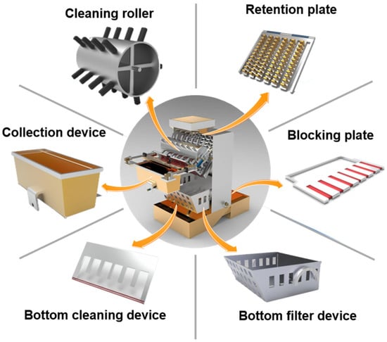
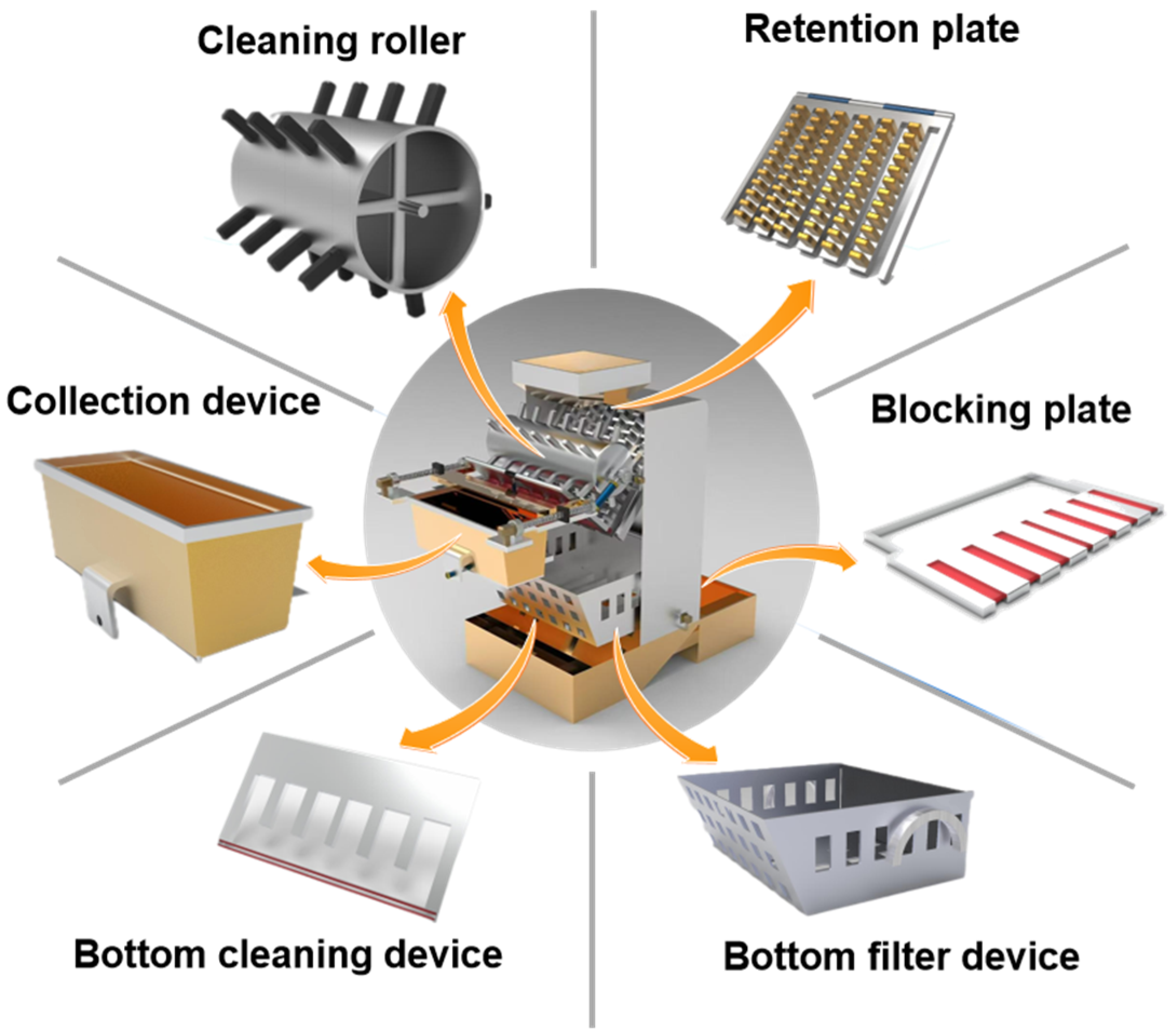
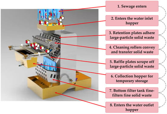
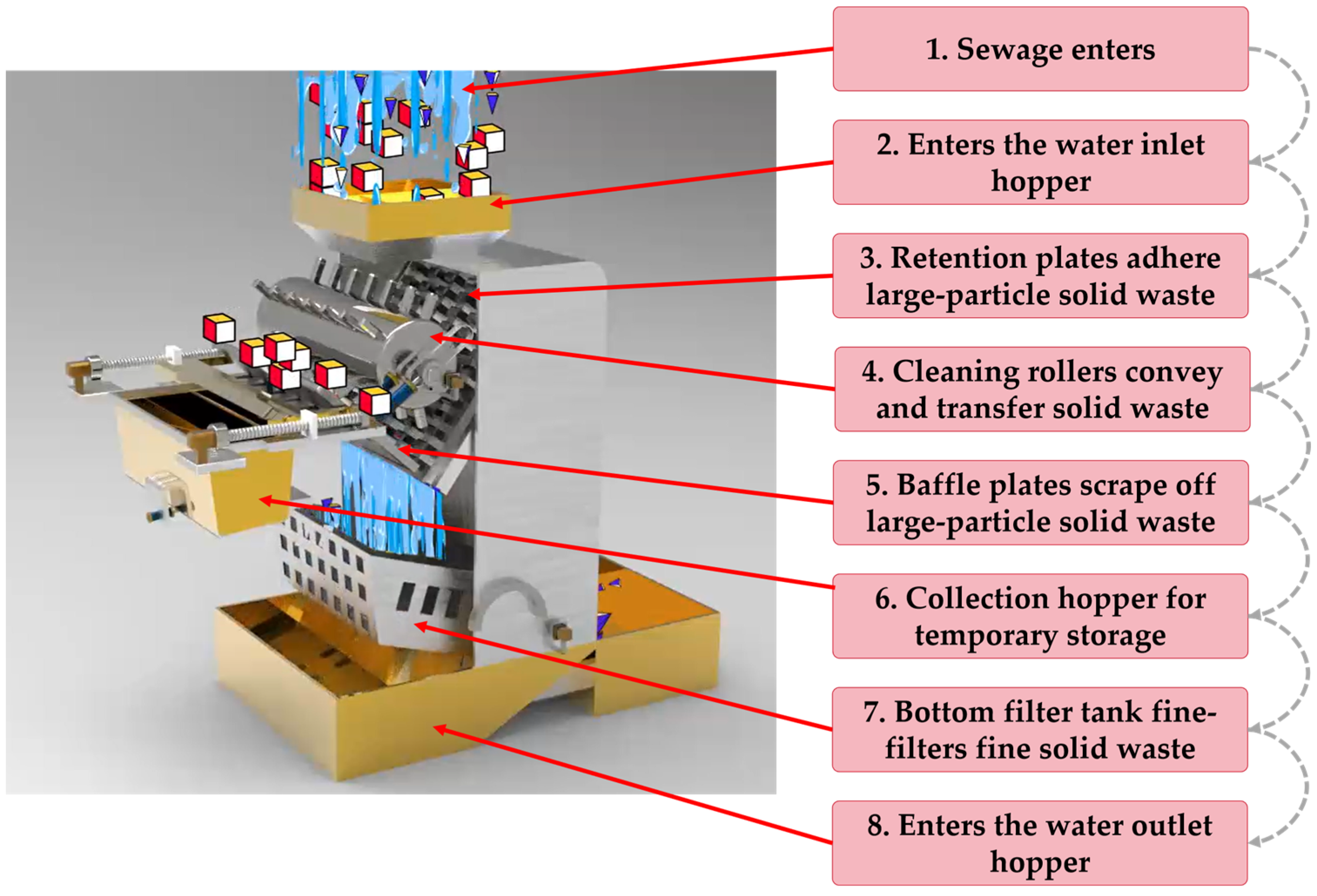
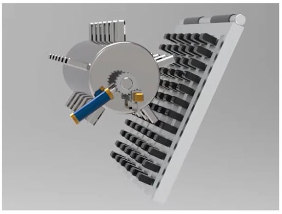
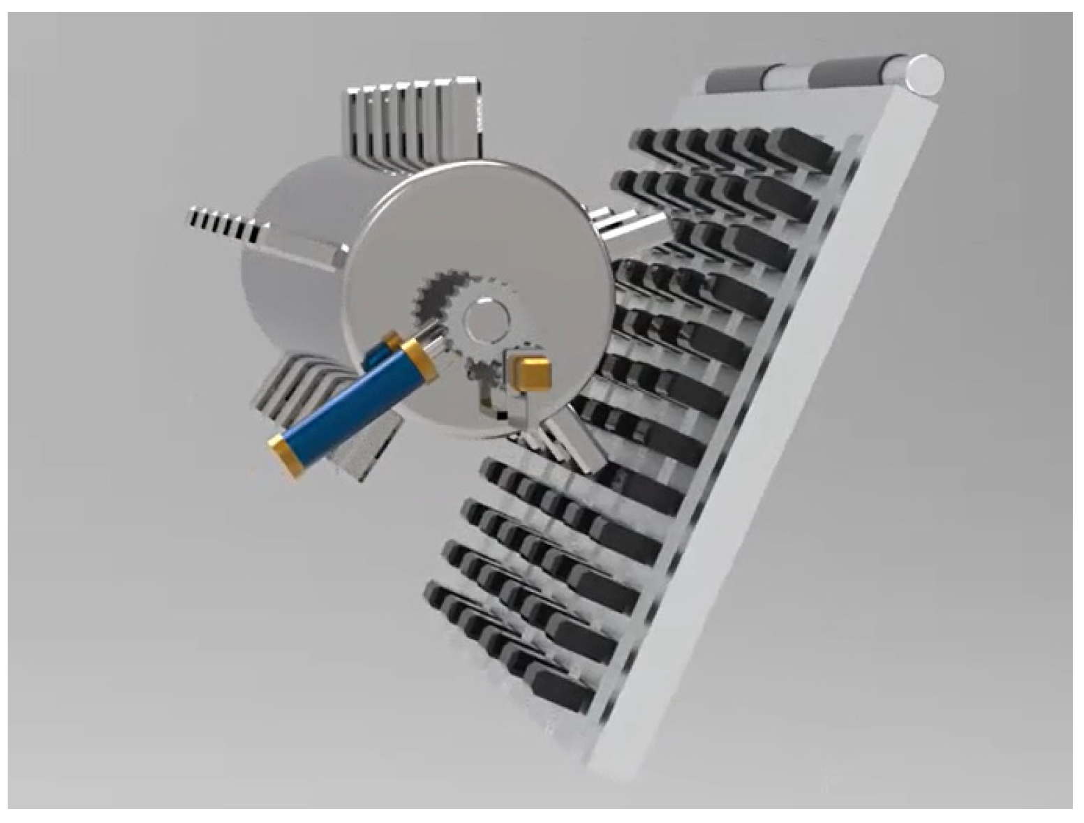
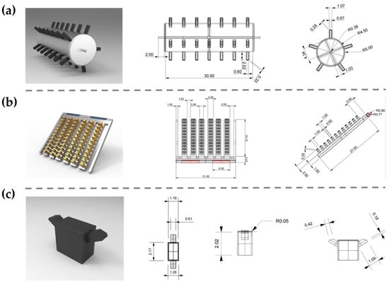
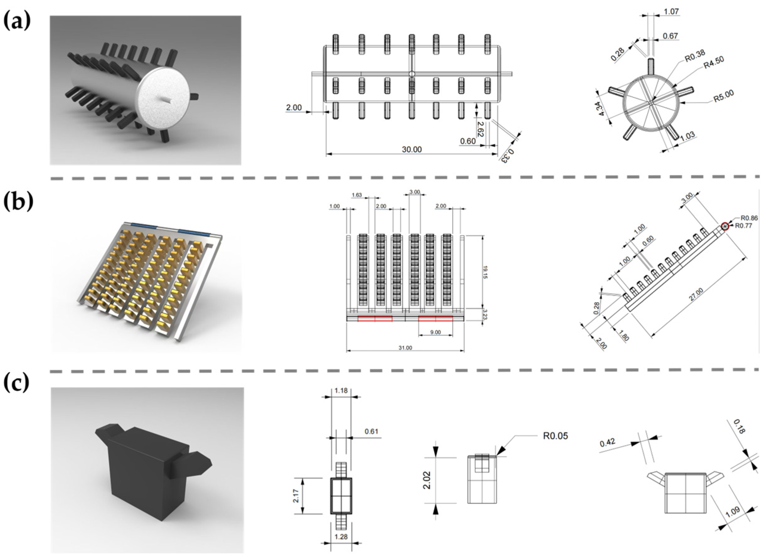
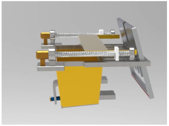
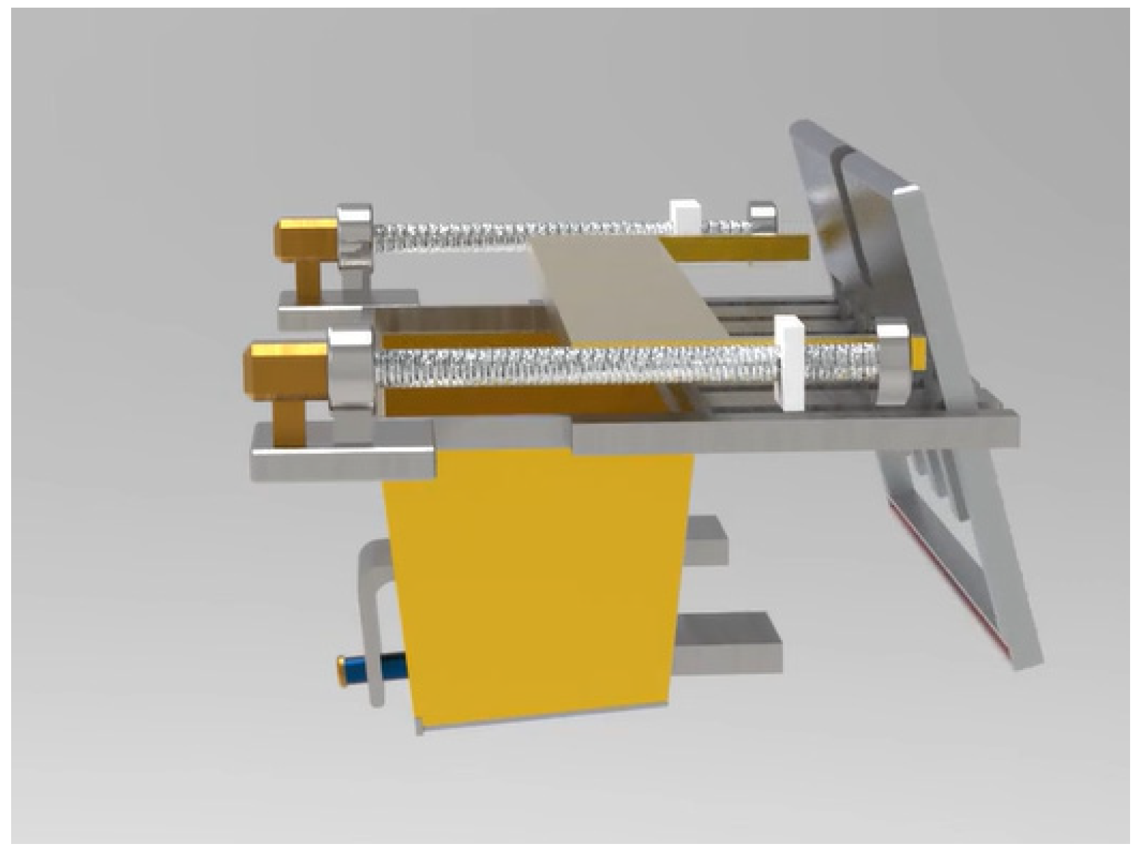
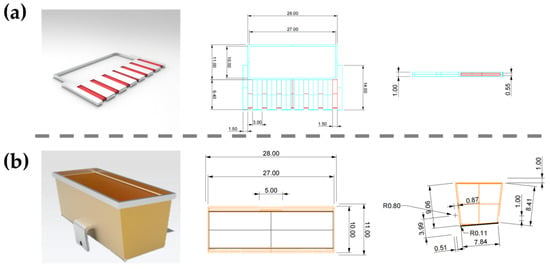
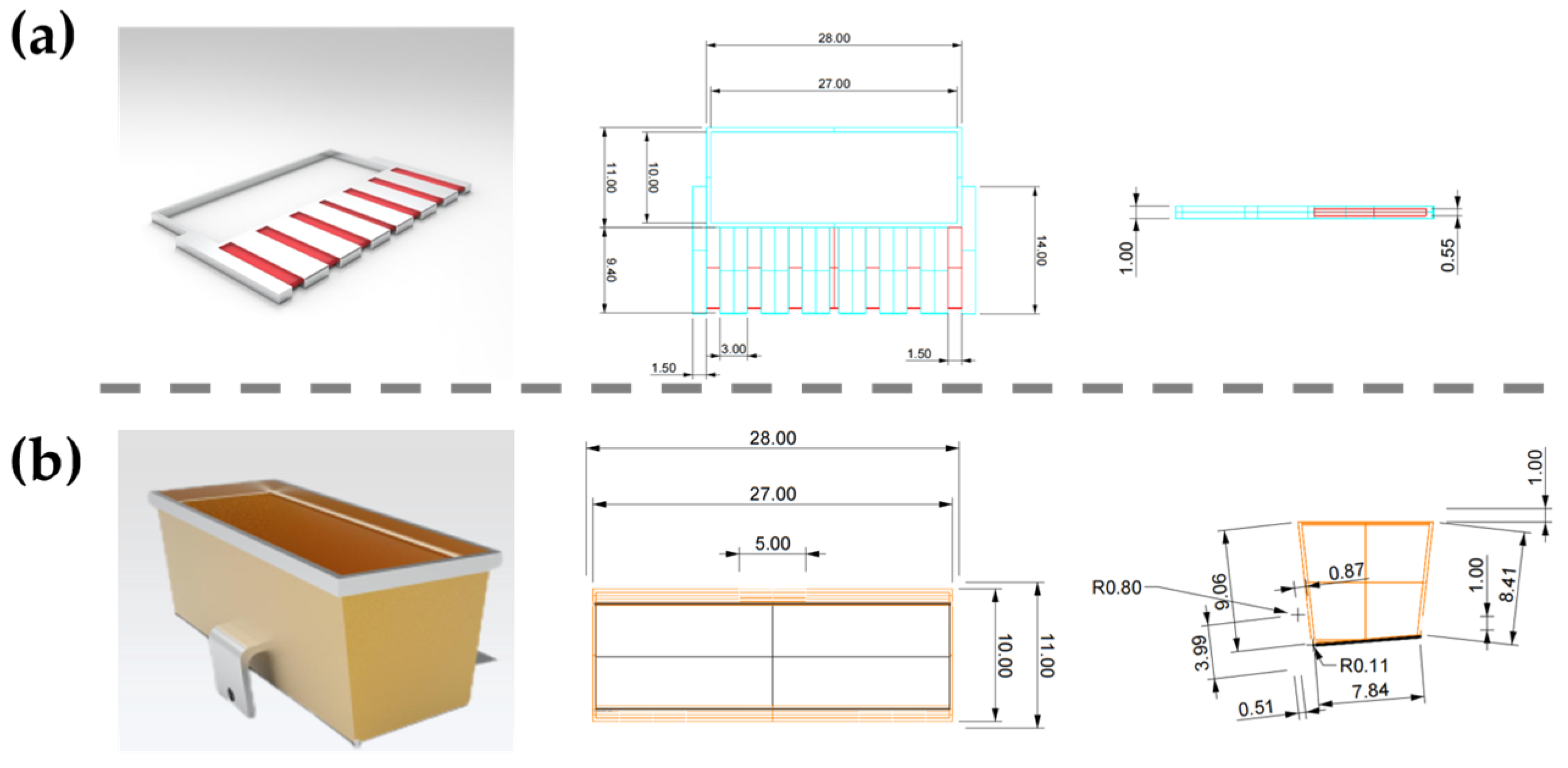
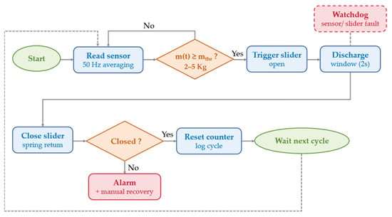
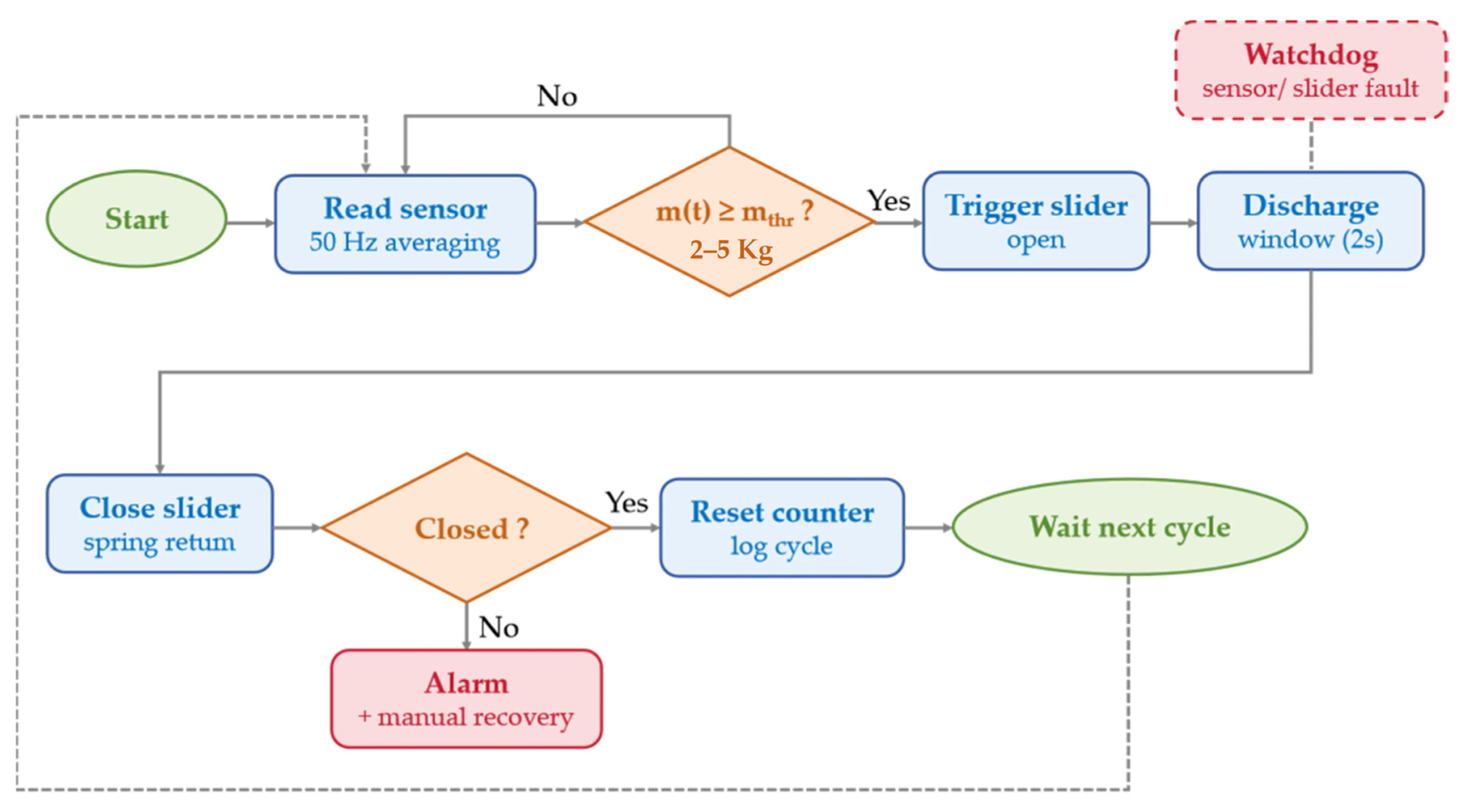
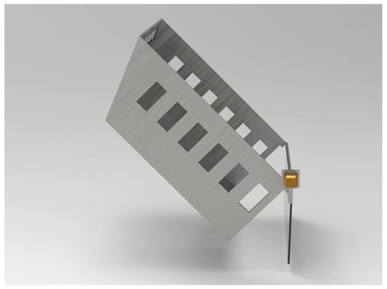
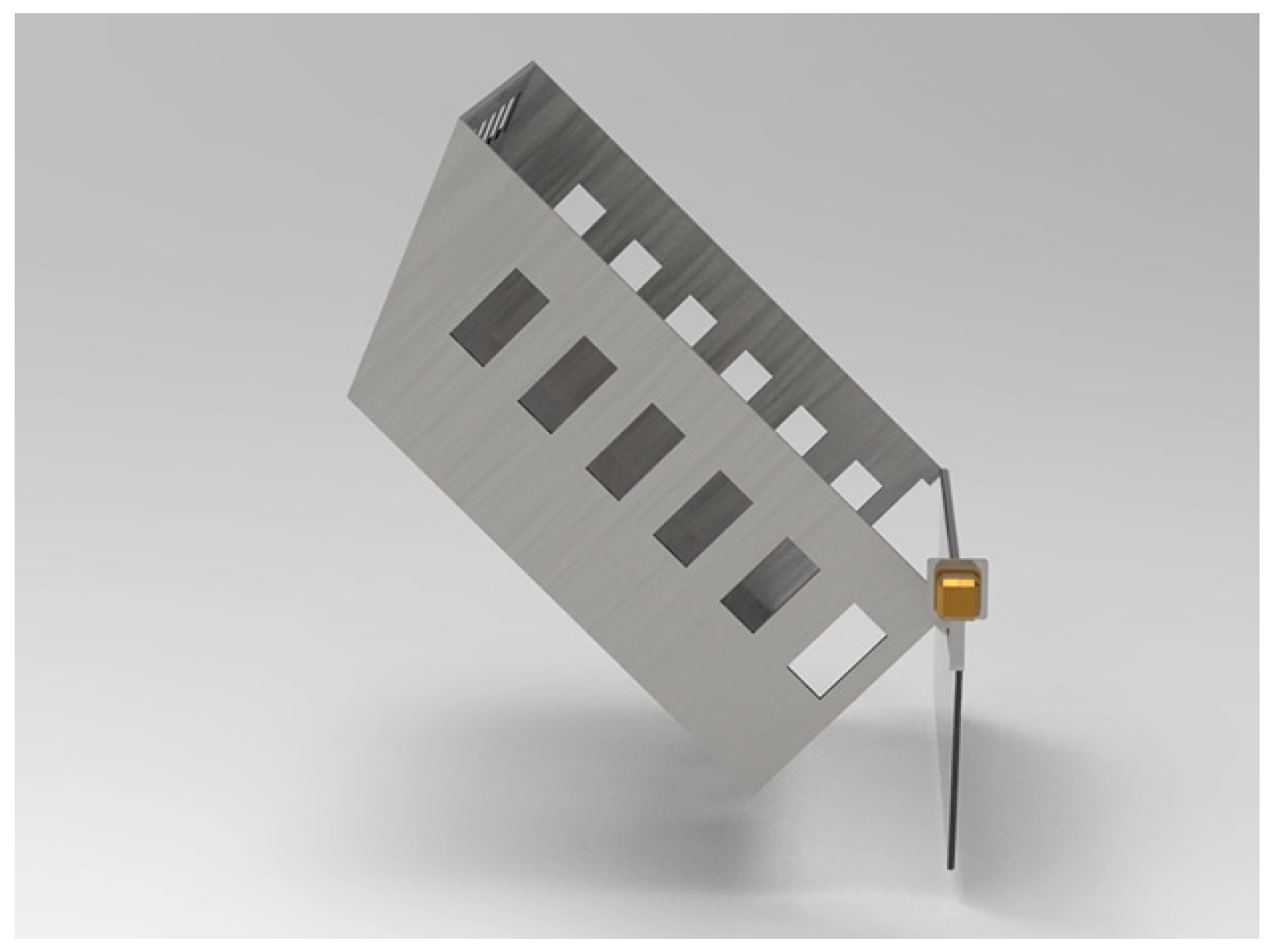
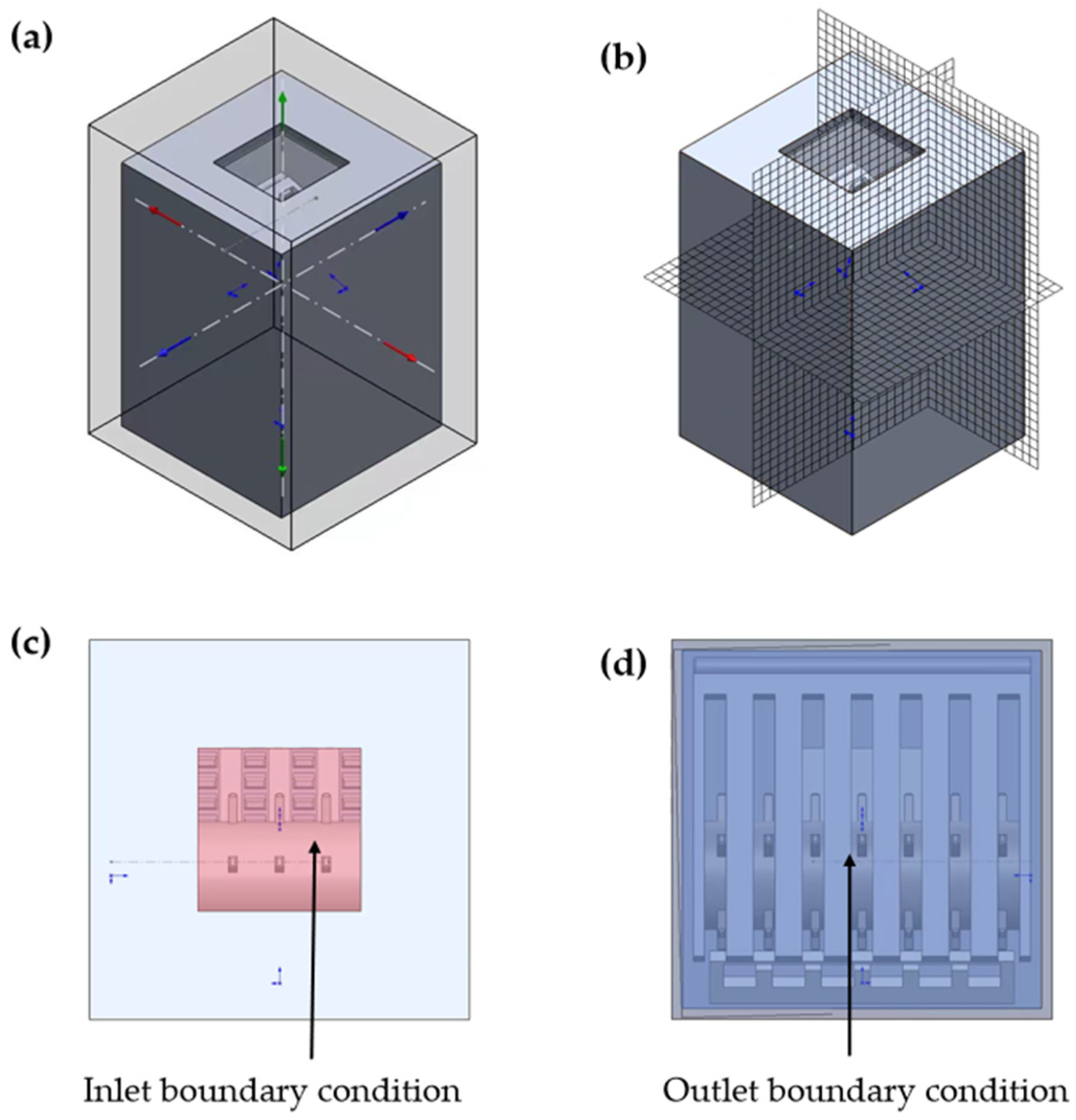
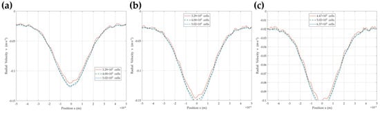
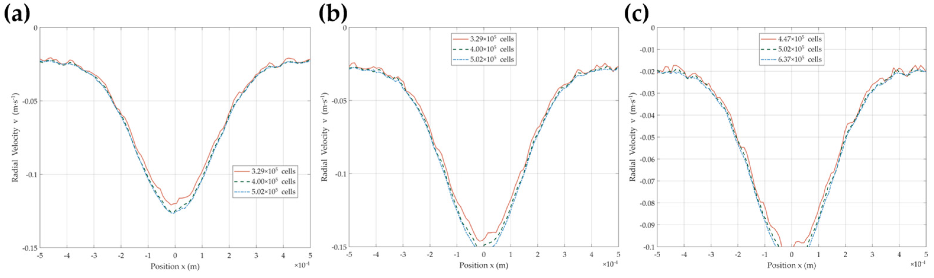
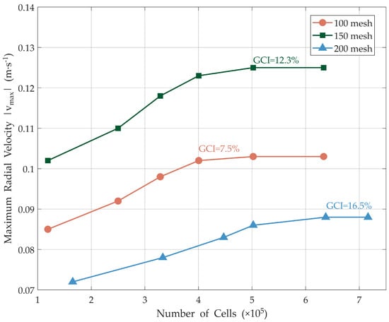
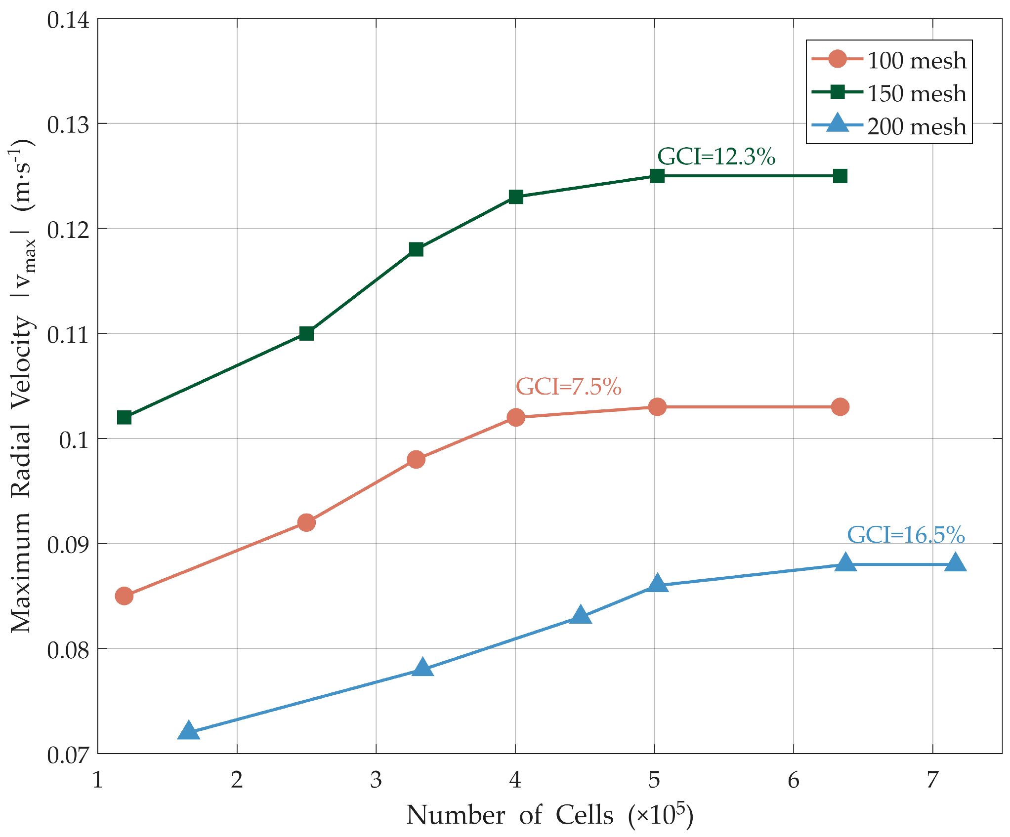
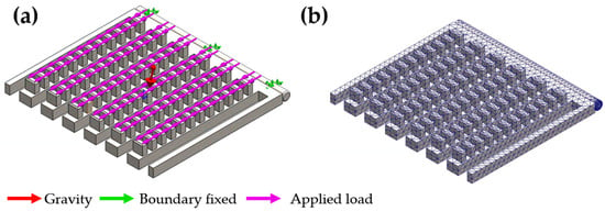
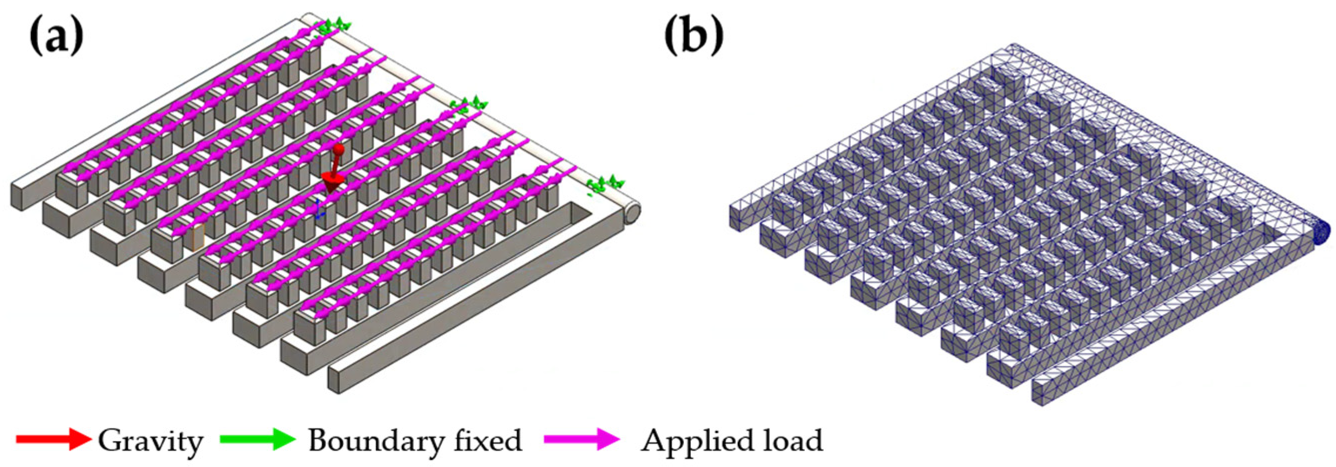
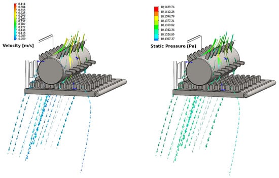
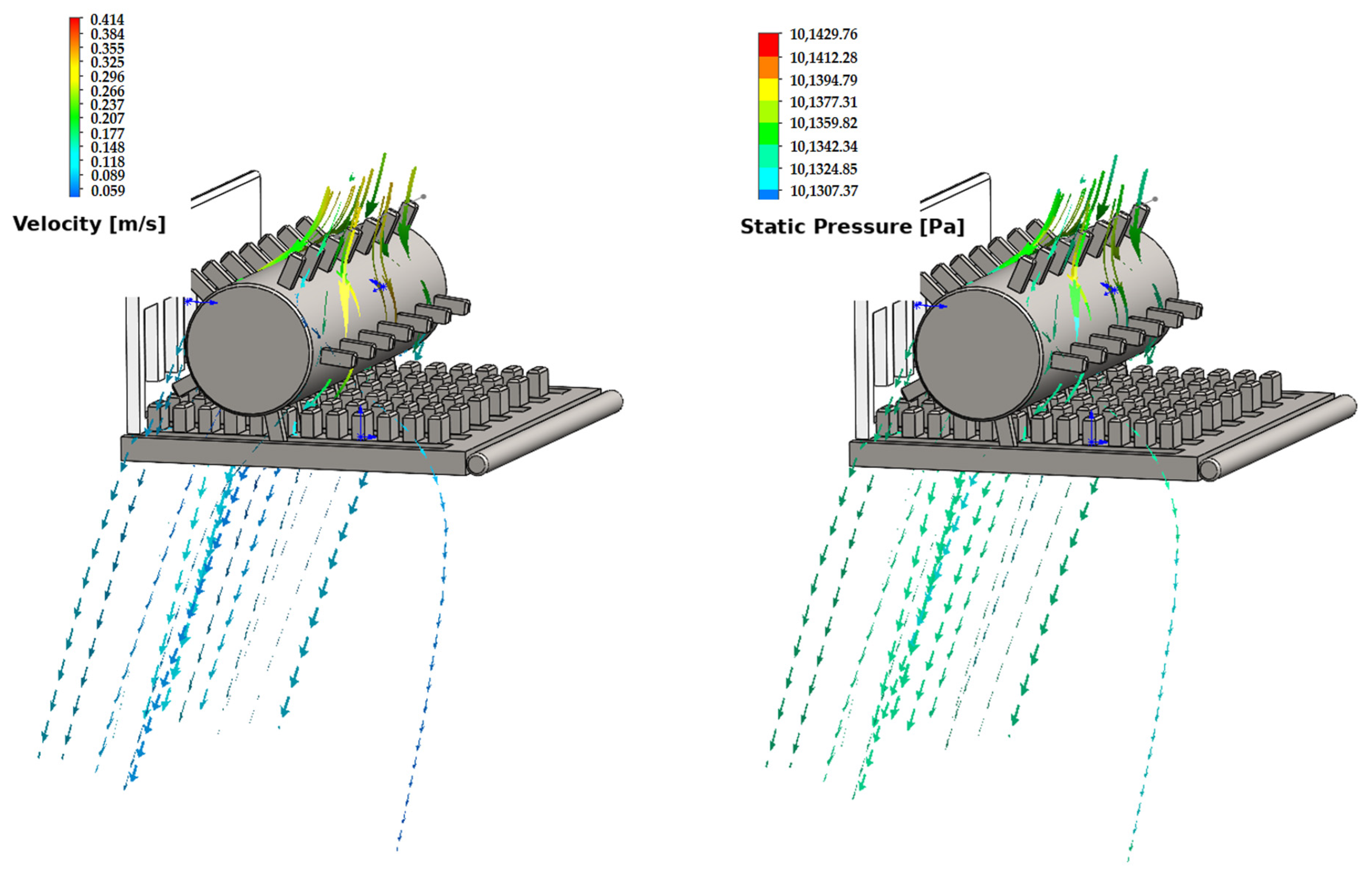
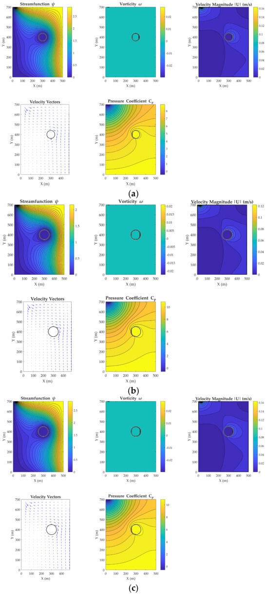
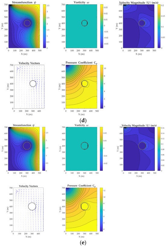
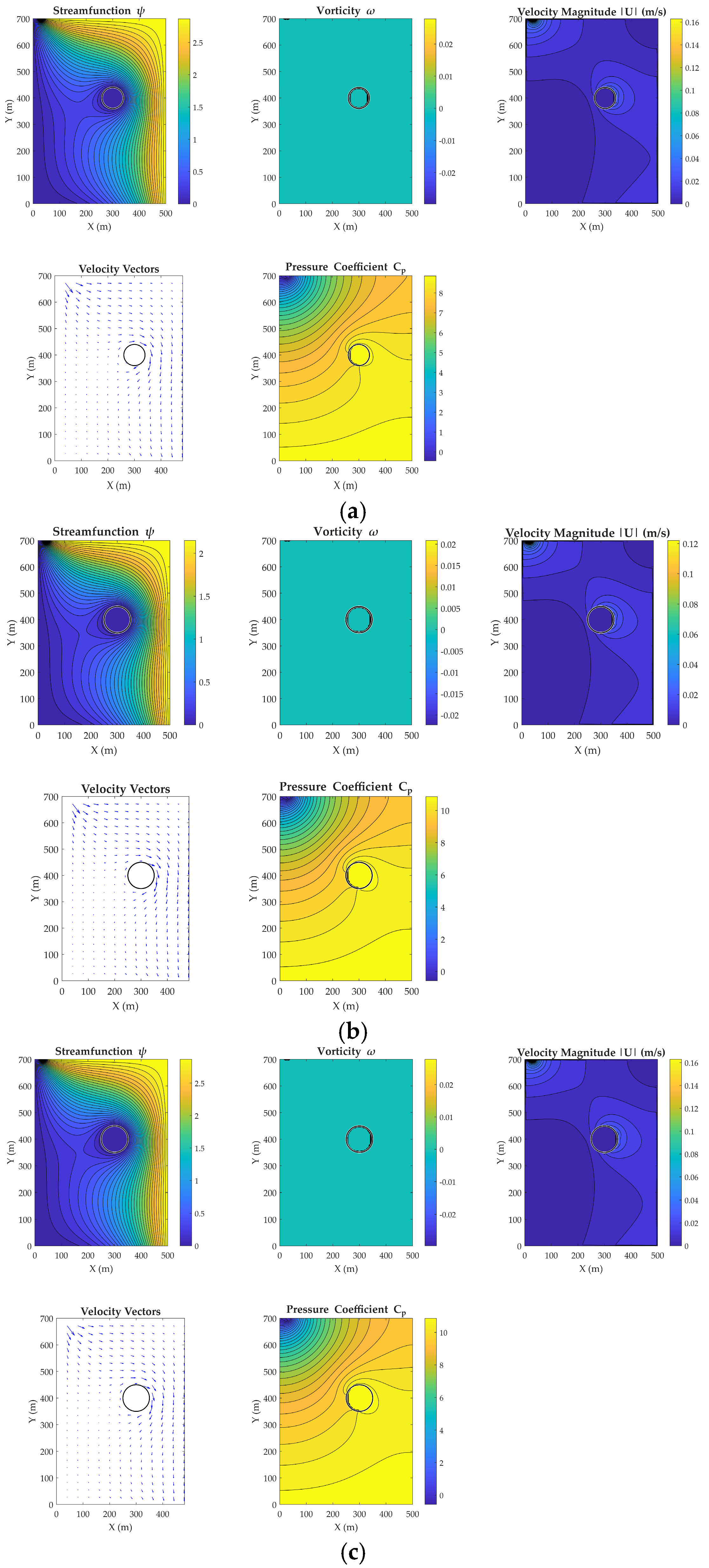
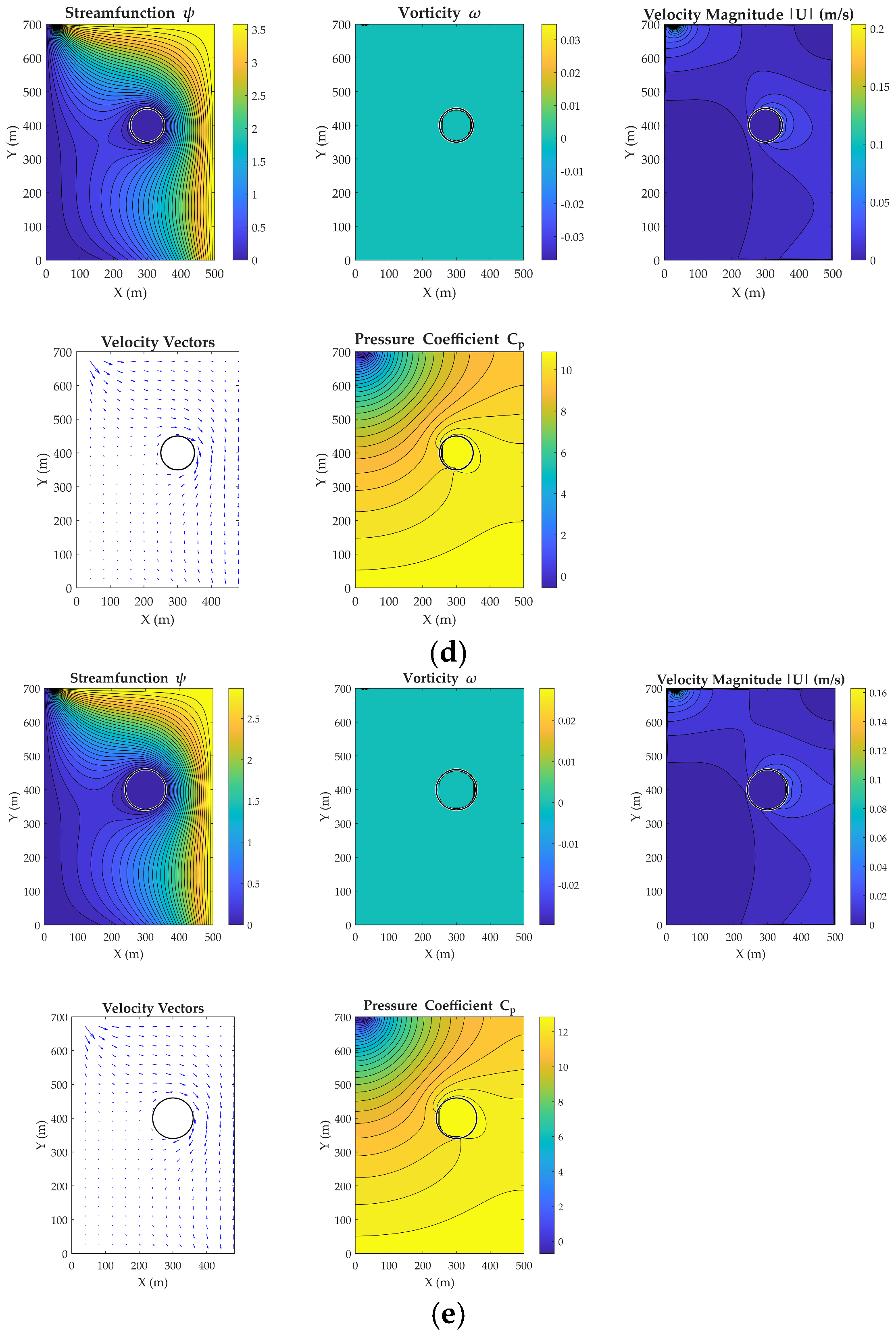
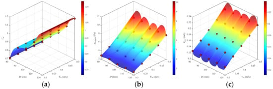
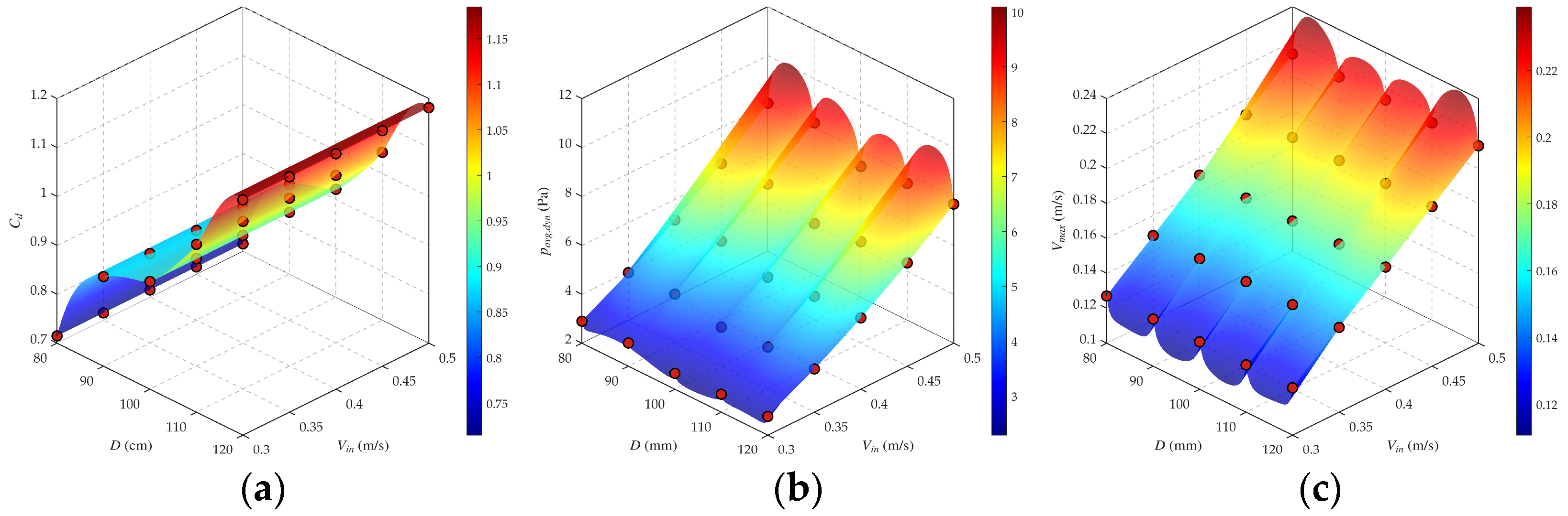
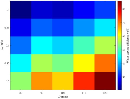
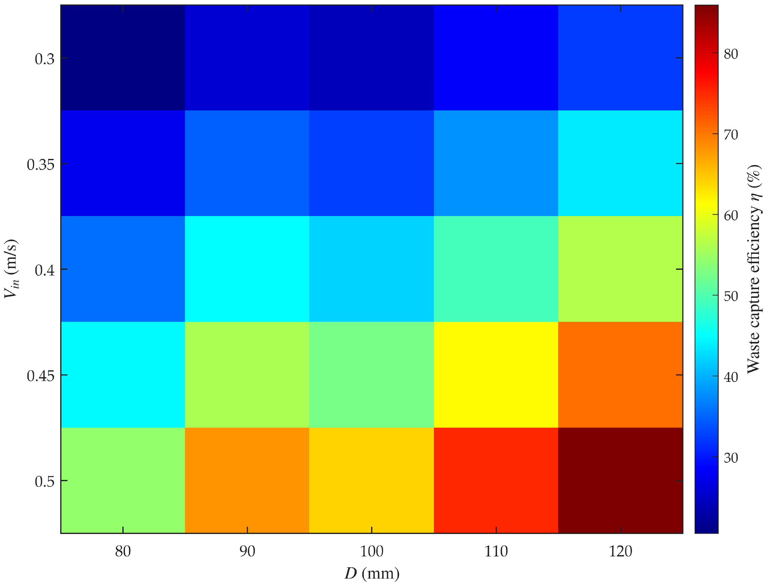
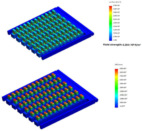
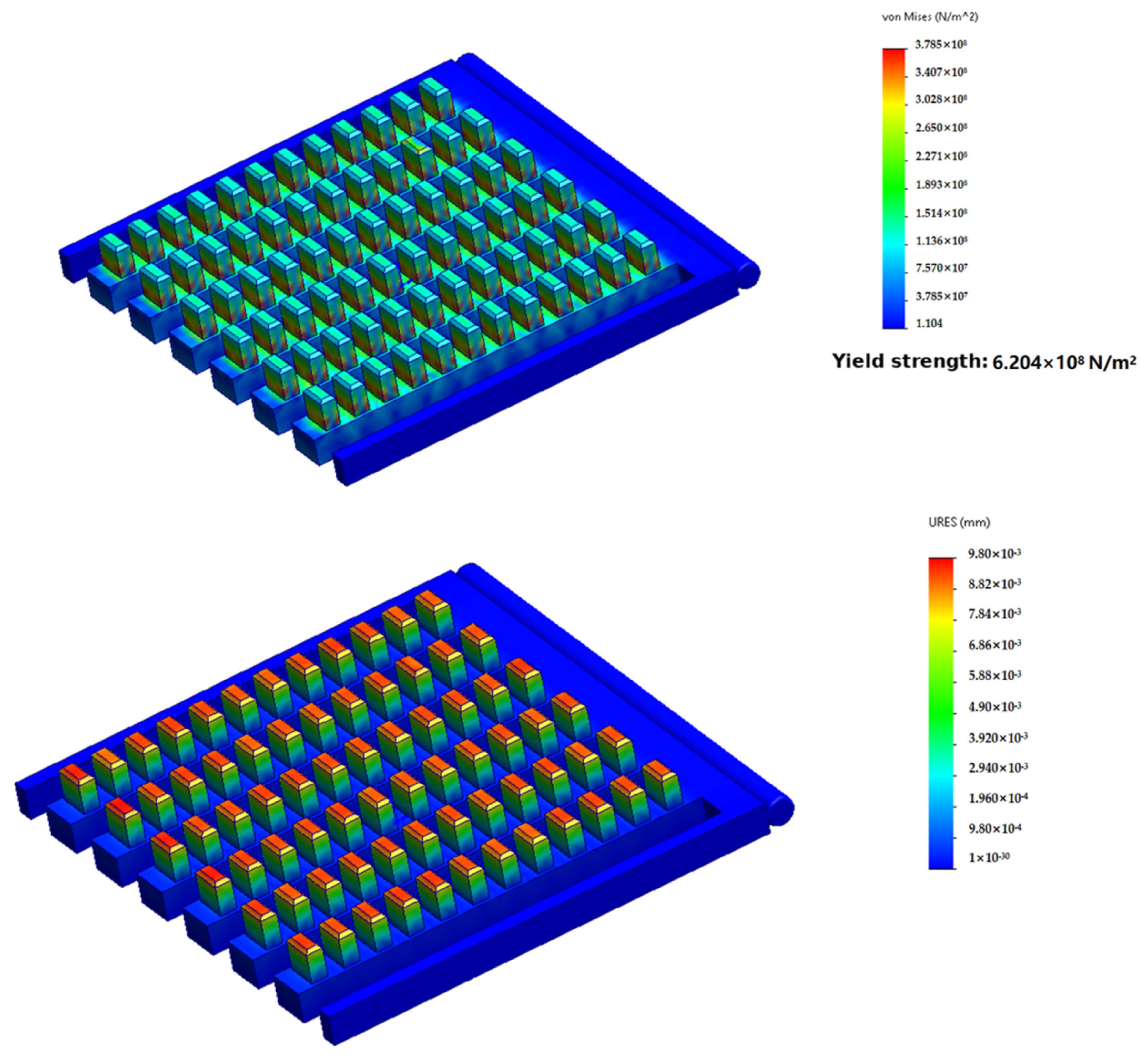
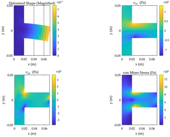
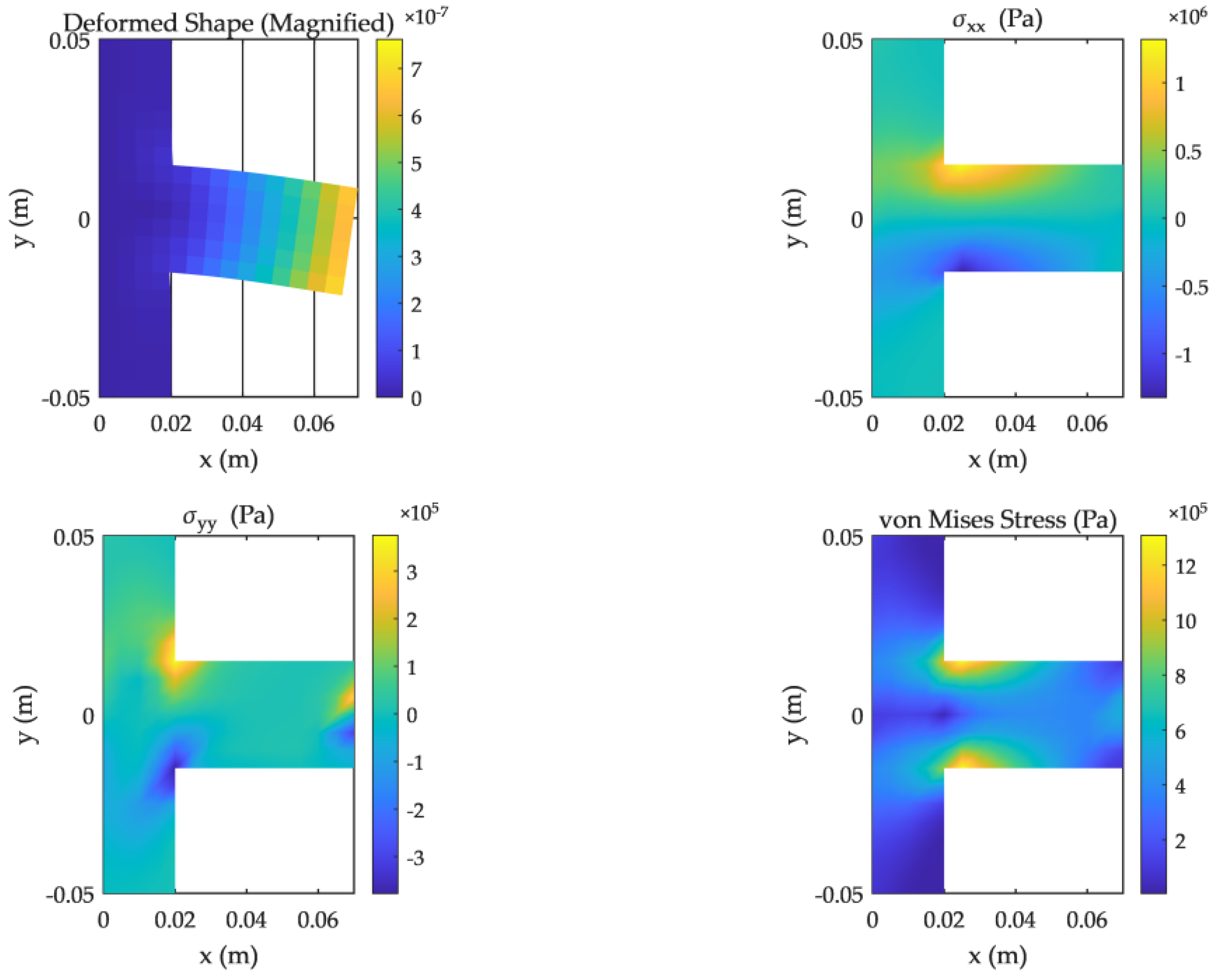
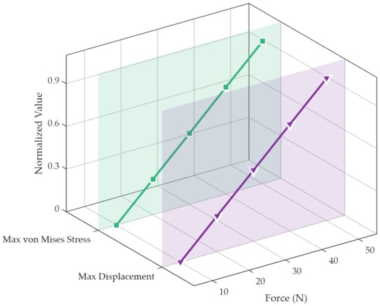
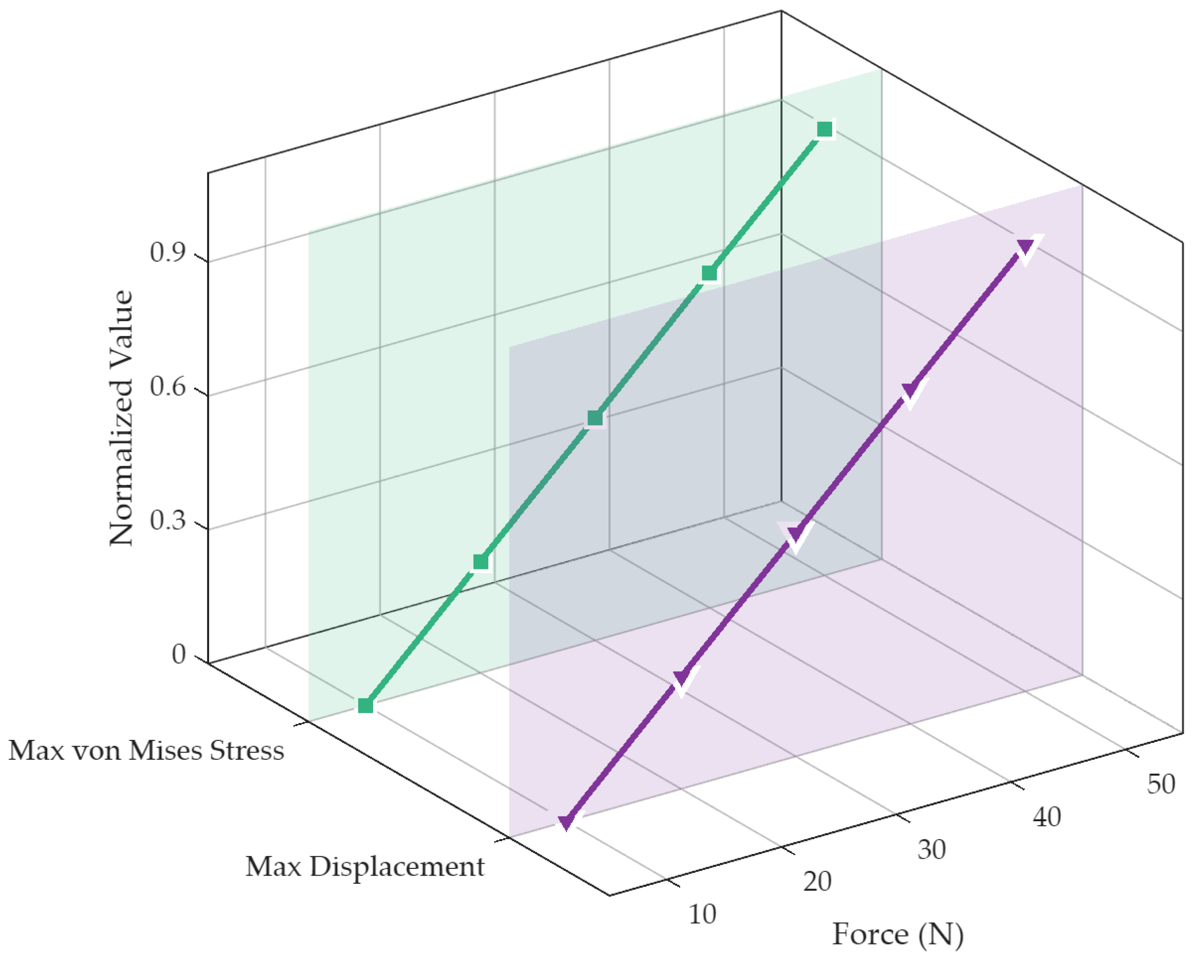
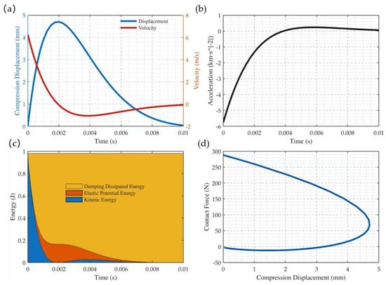
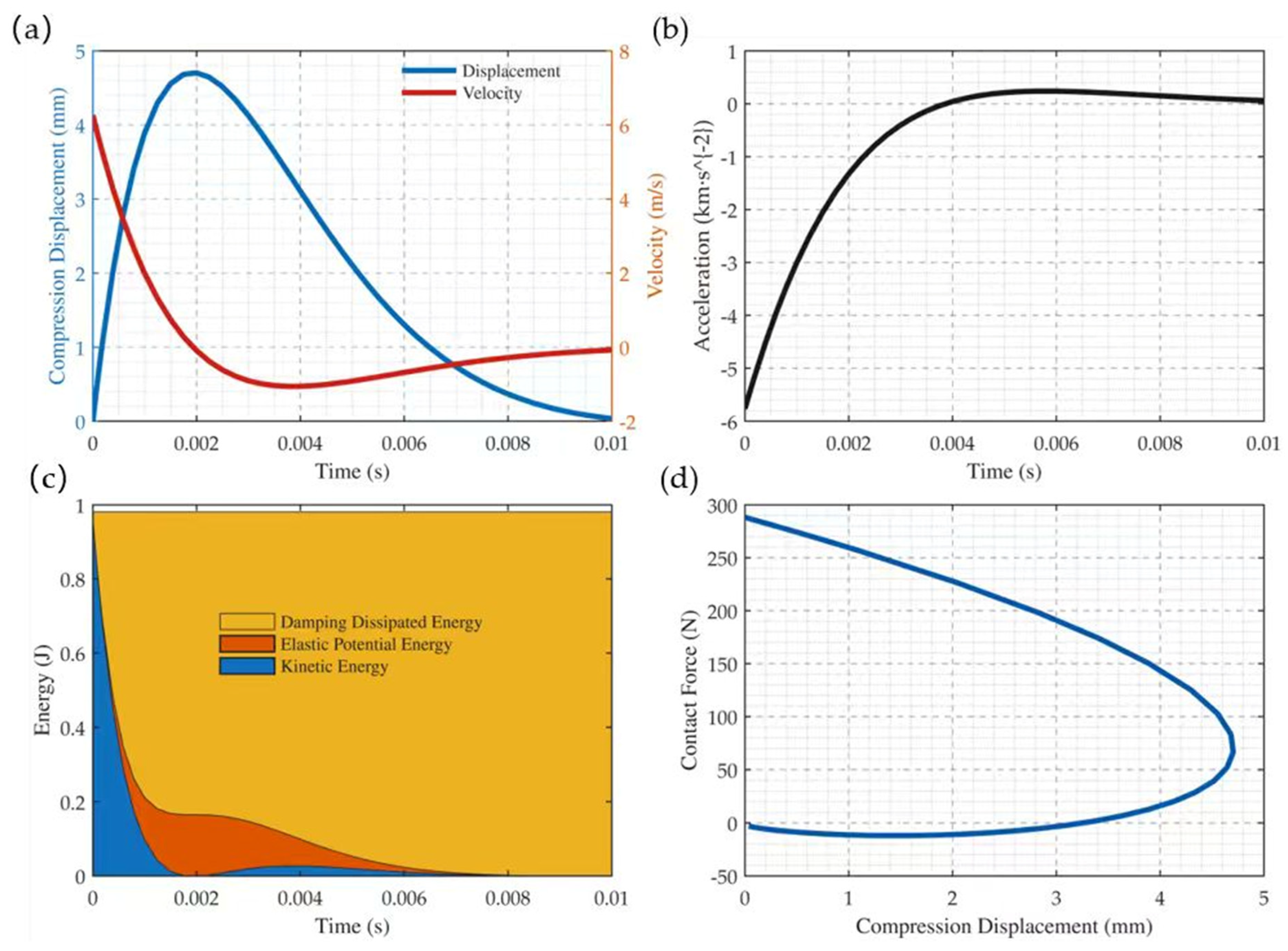
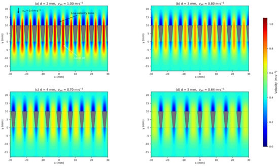
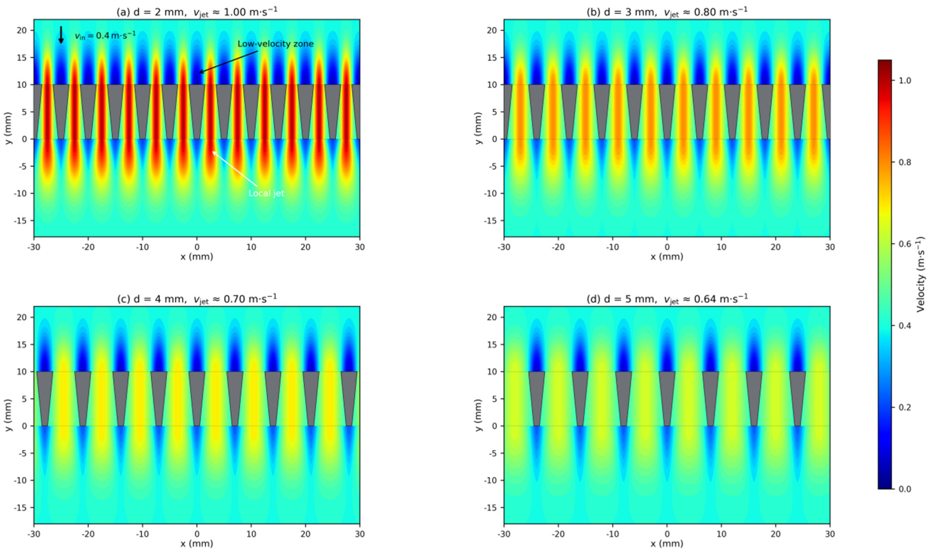
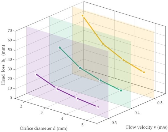
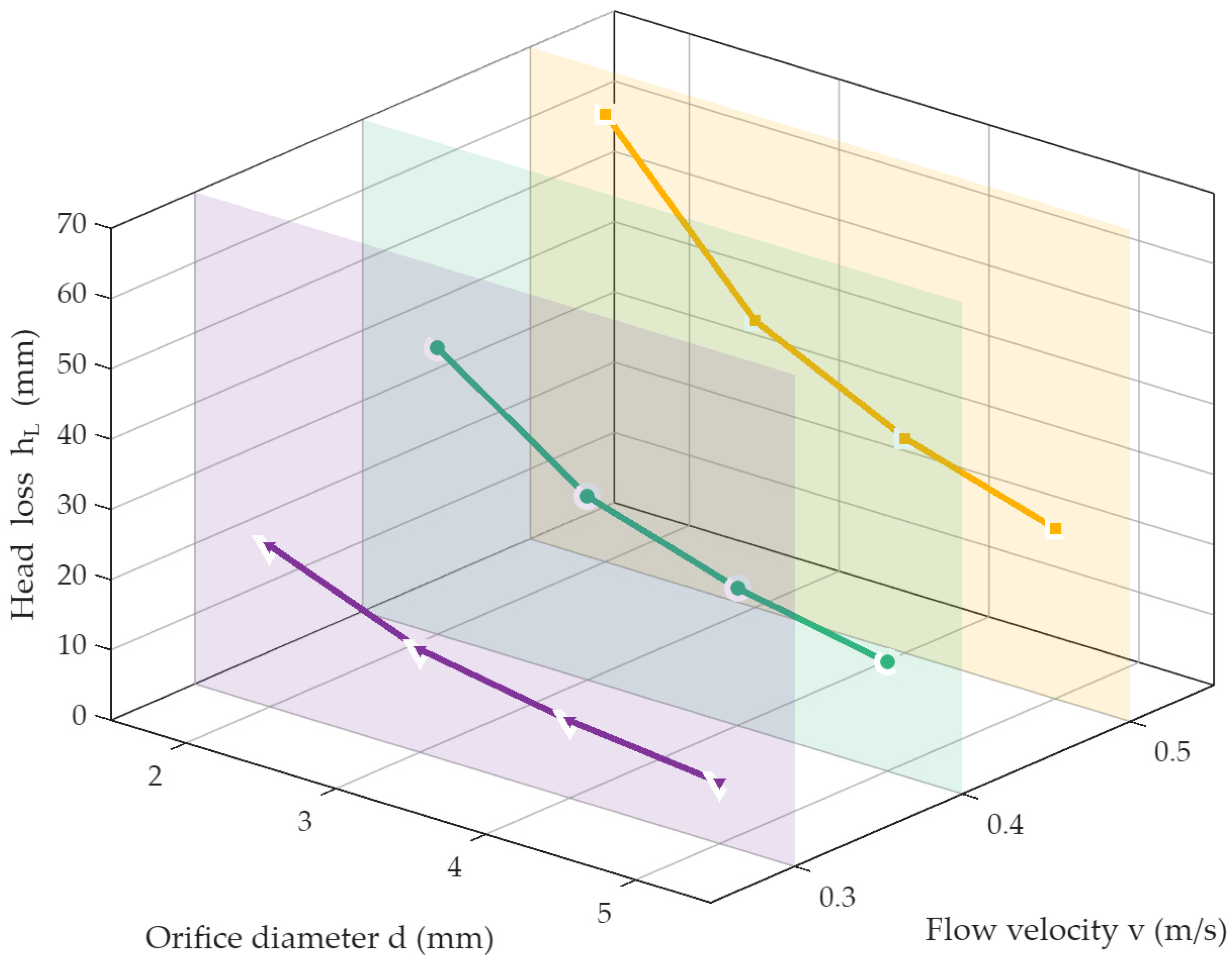
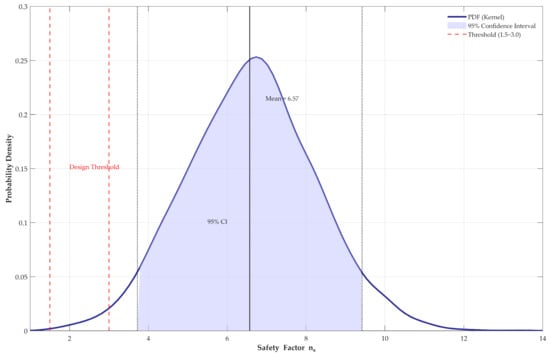
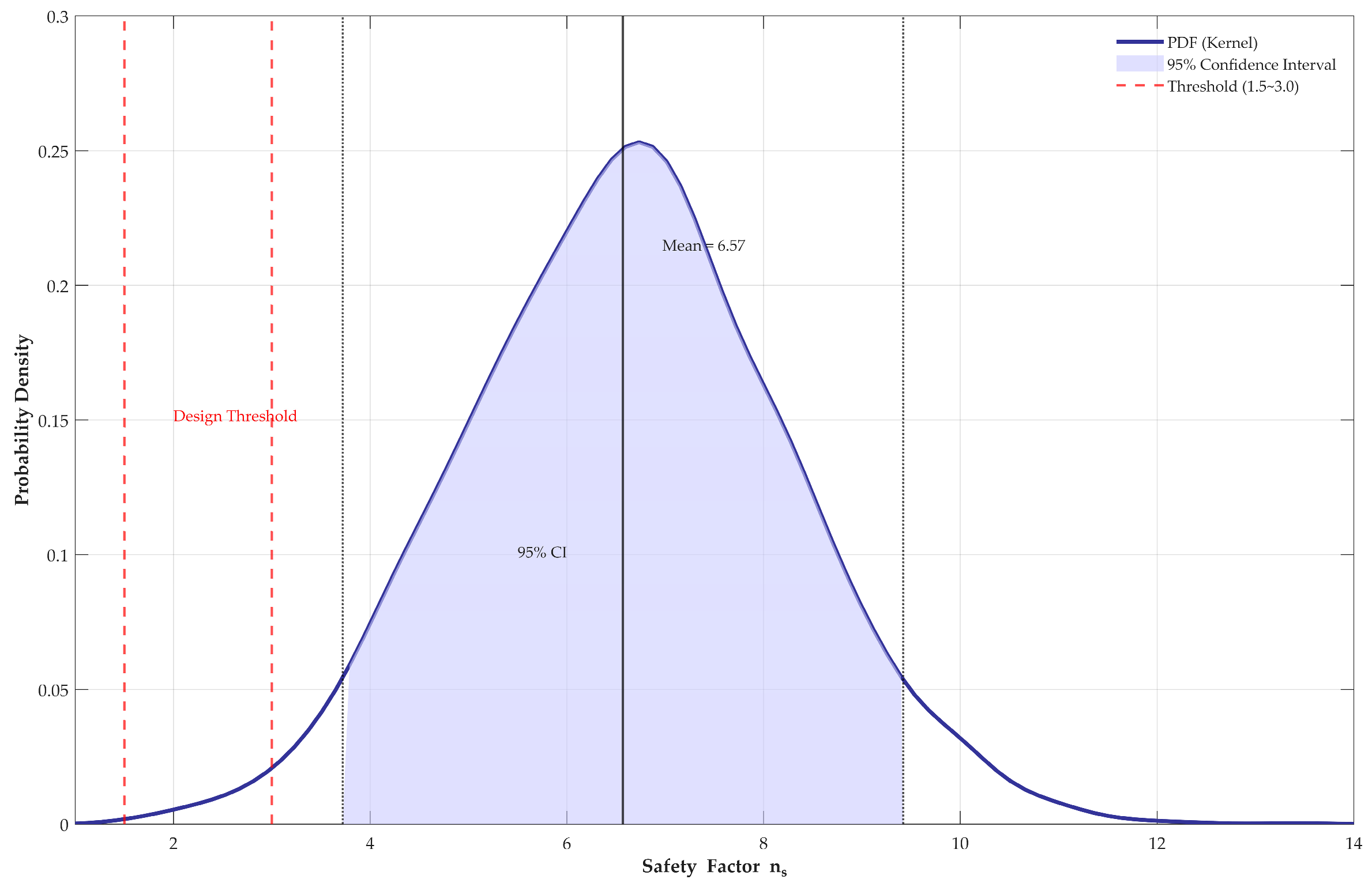
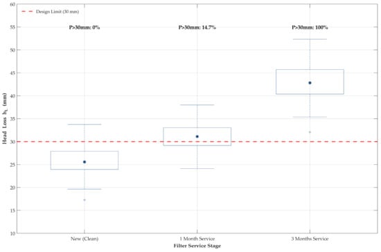
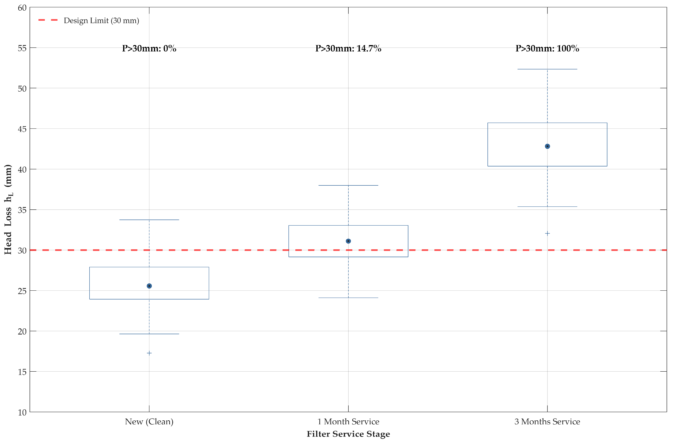
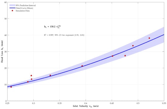

Disclaimer/Publisher’s Note: The statements, opinions and data contained in all publications are solely those of the individual author(s) and contributor(s) and not of MDPI and/or the editor(s). MDPI and/or the editor(s) disclaim responsibility for any injury to people or property resulting from any ideas, methods, instructions or products referred to in the content. |
© 2026 by the authors. Licensee MDPI, Basel, Switzerland. This article is an open access article distributed under the terms and conditions of the Creative Commons Attribution (CC BY) license.