Numerical Investigation of Cavitation Dynamics and Hydraulic Flip Transition in an Internal Nozzle

Abstract

This paper presents a numerical investigation of the cavitation dynamics and hydraulic flip transition in a rectangular nozzle using an Eulerian–Eulerian two-fluid model. The Schnerr–Sauer cavitation model was employed, with its key parameter—the initial bubble number density—set to 10¹⁴ m⁻³ based on experimental data to match the incipient cavitation and regime transition pressures accurately. Combined with a modified Reynolds-averaged Navier–Stokes turbulence model that incorporated the bubble-induced viscosity, this approach significantly improved the prediction accuracy of the mean flow field. The results revealed the quasi-periodic evolution from sheet to cloud cavitation, showing that the dominant frequency of cavity oscillations decreased with increasing inlet pressure. In contrast, the growth of sheet cavitation was the primary source of liquid turbulent kinetic energy. Furthermore, the complete transition sequence from super-cavitation to hydraulic flip was captured, elucidating the underlying vapor–air mixing mechanism. Analysis indicated that the hydraulic flip establishment time decreased sharply with the pressure before plateauing. In contrast, its thickness remained largely insensitive to the pressure and was governed by the upstream geometric configuration. The findings provide a calibrated and validated numerical framework for understanding complex cavitation mechanisms and optimizing spray system designs.

1. Introduction

There is an increasing interest in liquid jet atomization, which has been extensively utilized across various domains, including aeronautics, energy, propulsion, heat transfer, and materials processing. For instance, in internal combustion engines, liquid fuels are injected at high pressures to enhance jet break-up and achieve a high-quality fuel–air mixture. The nozzle orifice, which connects the upstream liquid supply system with the downstream injection atomization, is a key component influencing the droplet behavior and trajectories, ultimately affecting the combustion and emission performance. The rapid changes in the flow state within the orifice have a profound impact on the downstream atomization and combustion efficiency, particularly during fluctuations in the operating conditions and injector switching. Consequently, it is imperative to investigate the flow state variation process within the orifice to optimize the nozzle structure and improve the spray performance.

Multi-regime phenomena frequently arise within the nozzle due to variations in the operating conditions and differing injector designs. These regimes encompass turbulence, cavitating flow, and hydraulic flip, each characterized by distinct gas–liquid states within the nozzle orifice [1,2,3]. The regime transition process is highly sensitive to the prevailing operating conditions. In contrast to the turbulence and hydraulic flip regimes, cavitation within the internal nozzle exhibits a pronounced transient nature. Cavitation is a phase-change phenomenon that is influenced by hydrodynamic factors in high-velocity liquid flows, wherein the local static pressure experiences a rapid decline to the saturated vapor pressure. This abrupt change results in significant pressure fluctuations, as well as the generation of noise, vibrations, and erosion during the process of spray atomization.

1.1. Cavitation

Researchers have studied cavitation in internal flow channels through visualization experiments, revealing a quasi-periodic transition from sheet to cloud cavitation. Sheet cavitation refers to a thin, attached vapor film that forms on the solid boundary, while cloud cavitation describes the shedding of large, coherent vapor clusters into the core flow. Recent advances in fast synchrotron X-ray imaging have allowed simultaneous acquisition of the velocity and gas volume fraction fields, enhancing our understanding of the cavitation structure and flow dynamics [4]. Zhang et al. analyzed sheet growth and cloud shedding in a Venturi channel, noting differences at various inlet pressures [5]. Contrary to common belief, a weak re-entrant flow penetrates the entire cavity during globally steady sheet cavitation [6]. Cavitation modifies the mean velocity field, affecting the velocity fluctuations due to the correlation between the velocity gradients and turbulence intensity [7]. While long internal flow channels enable qualitative visualization of the cavitation behavior and its impact on the liquid velocity and turbulence intensity, capturing these effects in short injector orifices remains challenging. Investigating cavitation structures and flow characteristics in real nozzles is challenging and costly due to their intricate, micron-scale design.

1.2. Nozzle Flow Simulation Models

Numerical methods offer a cost-effective and efficient way to analyze the internal flow within a nozzle [8,9]. Dai et al. [10] examined the impact of curved nozzles on cavitation using the volume of fluid (VOF) multiphase flow model, integrating the k-ε turbulence and Schnerr–Sauer cavitation models. Sou et al. [3] combined the large eddy simulation (LES) method, the Eulerian–Lagrangian bubble tracking method (BTM), and the Rayleigh–Plesset equation to simulate incipient cavitation, revealing that the angle between the orifice wall and sac significantly affects cavitation development [11]. Zhu et al. [12] investigated the cavitating flow of liquid hydrogen using a compressible framework based on the homogeneous mixture model and the LES method. Mohand et al. [13] employed the homogeneous relaxation model (HRM) with the VOF and RNG (renormalization group) k-ε models to simulate nozzle flow, focusing on vaporization mechanisms related to cavitation and flash boiling. Mahmoud et al. [14] applied a mixture multiphase model with the Schnerr–Sauer cavitation model and the LES method to address the three-dimensional isothermal two-phase flow problem in nozzle flow, identifying trends in the turbulence kinetic energy and gas volume fraction at various pressure ratios.

Most multiphase models in nozzle simulations use the mixture hypothesis, which fails to adequately capture interactions between the air, vapor, and liquid phases. Understanding the interactions between the liquid and gas phases is crucial for analyzing air suction phenomena, particularly during cavitation and liquid boundary layer separation in hydraulic flips. Although mixture models require fewer experimental closure relations, accurately representing interfacial forces demands a well-resolved interface and turbulent structures, often necessitating computationally intensive techniques.

The two-fluid model (TFM) with the Eulerian–Eulerian approach is particularly adept at analyzing transient phenomena, wave propagation, and flow regime variations, especially when phases exhibit weak coupling and rapidly changing inertial properties [15]. In nozzle flow, liquid and vapor phases show weak coupling during cavitation and hydraulic flip regimes. Consequently, the local behavior of each phase during these transitions was emphasized in this study, and the TFM was adopted as the foundational framework for our multiphase analysis.

Turbulence modeling is essential for accurately capturing cavitation phenomena in nozzle flow [16,17]. The Reynolds-averaged Navier–Stokes (RANS) model, which is grounded in Boussinesq’s assumptions, is the most widely utilized approach due to its cost-effectiveness and robustness. This model has demonstrated strong performance in simulating bubbly flows, particularly in predicting cavitation flow [10,18,19]. Furthermore, the effects of bubble motion and liquid displacement warrant special consideration. Rzehak et al. observed that bubble-induced turbulence can significantly influence simulation outcomes in bubbly flow [20]. Maniscalco et al. found that LES models that incorporate this turbulence yield superior results across various conditions [21]. The role of bubble-induced turbulence is critical for enhancing the accuracy of multiphase turbulence predictions [22]. Consequently, the effects of bubble-induced turbulence were incorporated into the turbulence model in this study.

The cavitation model in nozzle flow elucidates the phase change and mass transfer occurring between two distinct phases. Prominent models, such as those proposed by Singhal [23], Schnerr–Sauer [24], and Zwart–Gerber–Belamri [25], utilize a simplified version of the Rayleigh–Plesset equation. The bubble number density is a critical parameter for cavitation initiation, with significant differences between fresh and contaminated fluids. Water quality affects the initial bubble number density, ranging from 10⁹ to 10¹⁵ nucleation sites per unit volume [26], a trend likely applicable to other liquids. Thus, the initial bubble number density was selected in this study based on prior experimental findings.

1.3. Super-Cavitation and Hydraulic Flip in Nozzle Flow

A prolonged cavity length at the nozzle exit can cause super-cavitation, a more unstable phenomenon than partial cavitation, where bubbles mix with external air, creating an air back-suction effect [27]. An increased cavity length often leads to hydraulic flip, particularly in nozzles with low length-to-diameter ratios, where a high-speed liquid forms a stable boundary layer that detaches from the wall before exiting, significantly impacting the near-nozzle spray characteristics. Research with transparent, symmetrically scaled nozzles [28,29,30] has indicated that hydraulic flip occurs when the flow rates increase to the point of wall detachment, resulting in a complete flow change without cavitation. An experiment with a gasoline direct injection (GDI) injector used X-ray phase contrast imaging to characterize hydraulic flip, showing that a nozzle with a rounded inlet edge produces a thinner hydraulic flip, resulting in a higher discharge coefficient and a lower turbulence intensity [31]. The nozzle’s internal flow comprises liquid, cavitation bubbles, and entrained air, transitioning from partial cavitation to super-cavitation or hydraulic flip. Most studies focused on either the partial cavitation or hydraulic flip regime, leaving the multifluid processes of super-cavitation and hydraulic flip flows underexplored.

Beyond the internal nozzle flows, substantial efforts have also been devoted to understanding the subsequent jet break-up and impingement processes, which are inherently linked to the initial in-nozzle flow conditions [32]. Furthermore, fundamental studies on cavitation phenomena in other high-speed fluid machinery, such as aerodynamic applications [33], provide complementary insights into the complex nature of phase-change dynamics. However, the intricate multi-fluid interactions during the super-cavitation and hydraulic flip regimes in injector nozzles remain underexplored.

In this study, the TFM multiphase model was used, along with a bubble-induced RANS turbulence model and a parameter-adjusted S-S cavitation model, to investigate the dynamic evolution of nozzle flow regimes, from partial cavitation to hydraulic flip. The differences in the cavitation morphology and mechanisms under various operating conditions were analyzed, and the effects of dynamic cavitation oscillation on the fluid pressure, flow, and turbulence intensity were characterized. The study also provides insights into the transition to hydraulic flip, offering references for optimizing the injector design in liquid atomization technology.

The well-documented experimental dataset of Park et al. [34], which provides both flow visualization and global discharge coefficients for a transparent rectangular nozzle, serves as an ideal benchmark for validating our numerical framework. The adoption of this specific geometry is a prerequisite for a rigorous model validation, ensuring that our predictions can be directly and quantitatively compared against established measurements. However, the primary objective of this study is not to replicate their findings, but to leverage this validated geometry as a platform for a deeper physical investigation that was unattainable in the original experiments. While Park et al. focused on macroscopic flow regimes and atomization performance, our work extends the prior work by: (1) providing a detailed mechanistic analysis of the transient sheet-to-cloud cavitation dynamics, including quantitative Strouhal numbers; (2) elucidating for the first time the complete vapor–air mixing pathway during the super-cavitation to hydraulic flip transition using a two-fluid model; and (3) quantifying the establishment time and thickness of hydraulic flip, which were not accessible in the original experiments.

The novelty of this work lies in the application of a calibrated Eulerian two-fluid model that uniquely combines a bubble-induced RANS turbulence model with the Schnerr–Sauer cavitation model to investigate the detailed dynamics of the transition from partial cavitation, through super-cavitation, to hydraulic flip in a rectangular nozzle. This approach allows for an explicit analysis of phase interactions and provides new insights into the vapor–air mixing mechanisms governing the hydraulic flip establishment.

2. Numerical Methods

2.1. Nozzle Geometry and Mesh Topology

Park et al. [34] experimentally studied the internal cavitation and atomization performance using a transparent rectangular nozzle (6 mm length, 2 mm spanwise width) under varying inlet pressures. The rectangular design effectively reduces bubble formation on all walls except the side wall, thereby facilitating clearer observations of the cavitation dynamics from both the front and side perspectives.

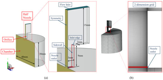
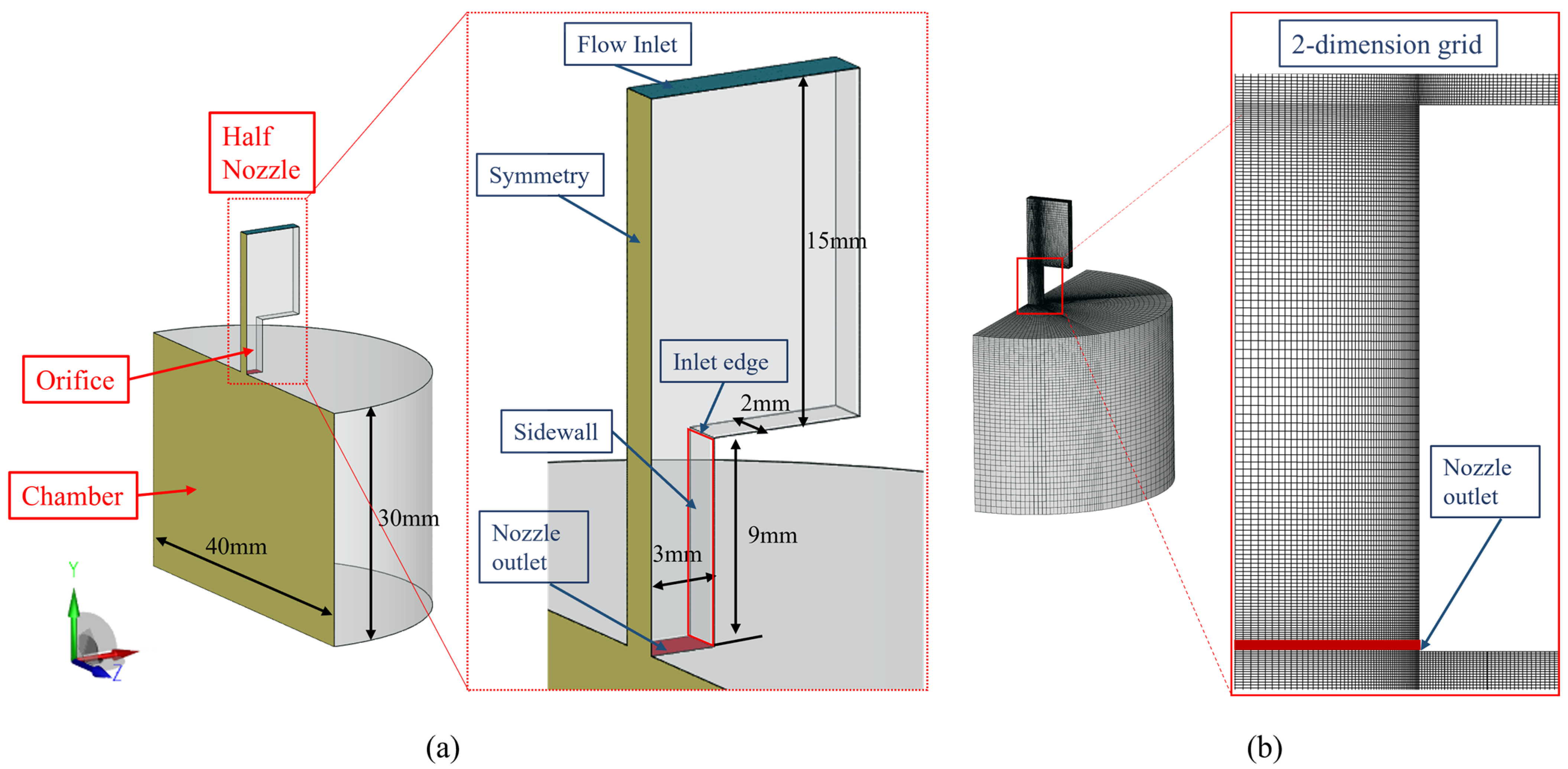
The present numerical study adopts this nozzle geometry. Taking advantage of geometric symmetry, the computational domain is reduced to one half of the full nozzle and the connected downstream chamber; both share a common, co-planar symmetry plane. Figure 1 illustrates the nozzle configuration, computational domain, and mesh. The three-dimensional half-domain with applied boundary conditions is shown in Figure 1a: the symmetry plane is colored yellow, the side wall is highlighted by a red outline, and the flow path from the inlet, past the nozzle inlet edge and along the side wall, to the nozzle exit and into the half-cylinder chamber is explicitly labeled. A symmetry condition (zero normal velocity and zero normal gradients) is prescribed on the symmetry plane, while the side wall and all remaining solid walls are treated as no-slip walls.

Figure 1. (a) Computational domain structure; (b) Grid details.

Figure 1b presents the structured hexahedral mesh, with local refinement applied at the nozzle inlet edge and along the side wall to adequately resolve high-gradient regions; the mesh connectivity at the nozzle inlet, nozzle exit, and chamber interface is clearly visible. Mesh refinements at the inlet edge and side wall were essential for ensuring accurate simulations.

2.2. Governing Equations

The Euler–Euler two-fluid multiphase model describes cavitation development and hydraulic flip transitions by treating each phase separately. It includes conservation equations for mass, momentum, and energy, with terms for phase interactions affecting the transfer processes. The nozzle’s internal flow may contain vapor from cavitation and air due to the low pressure, resulting in three phases: liquid, vapor, and air. The gas phase was treated as a homogeneous mixture of vapor and air, resulting in two phases (liquid and gas) in the governing equations. The liquid was assumed to be weakly compressible, with both phases sharing the same pressure. The mathematical model is detailed below.

• Continuity Equation:

The continuity equations for the gas and liquid phases are

$${\displaystyle \frac{\partial ({\alpha }_{\mathit{g}}{\rho }_{\mathit{g}})}{\partial t}}+\nabla \cdot ({\alpha }_{\mathit{g}}{\rho }_g{u}_{\mathit{g}})={\dot{m}}_{\mathit{lg}},\mathrm{where}{\alpha }_g={\alpha }_{vapor}+{\alpha }_{air}$$

(1)

$${\displaystyle \frac{\partial ({\alpha }_{\mathit{l}}{\rho }_{\mathit{l}})}{\partial t}}+\nabla \cdot ({\alpha }_{\mathit{l}}{\rho }_{\mathit{l}}{u}_{\mathit{l}})={\dot{m}}_{\mathit{gl}}.$$

(2)

where $\mathit{\alpha },\rho ,$ and u are the volume fraction, density, and velocity, respectively. The subscripts l and g denote the liquid and gas phases, respectively. In cavitation flow, ${\dot{m}}_{\mathit{gl}}$ and ${\dot{m}}_{\mathit{lg}}$ represent mass transfer source terms for condensation and evaporation due to cavitation, respectively. The relationship between the liquid and gas volume fractions is as follows: ${\alpha }_l+{\alpha }_g=1$.

• Momentum Equation:

The momentum balance equations for the two phases are

$${\displaystyle \frac{\partial ({\alpha }_{\mathit{g}}{\rho }_{\mathit{g}}{u}_{\mathit{g}})}{\partial t}}+\nabla \cdot ({\alpha }_{\mathit{g}}{\rho }_{\mathit{g}}{u}_{\mathit{g}}{u}_{\mathit{g}})=-{\alpha }_{\mathit{g}}\nabla P+{\alpha }_{\mathit{g}}\nabla \cdot {\tau }_g+{\alpha }_{\mathit{g}}{\rho }_{\mathit{g}}g+F_{\mathit{gl}}+(m_{\mathit{lg}}{u}_{\mathit{g}}-m_{\mathit{gl}}{u}_{\mathit{l}})$$

(3)

$${\displaystyle \frac{\partial ({\alpha }_{\mathit{l}}{\rho }_{\mathit{l}}{u}_{\mathit{l}})}{\partial t}}+\nabla \cdot ({\alpha }_{\mathit{l}}{\rho }_{\mathit{l}}{u}_{\mathit{l}})=-{\alpha }_{\mathit{l}}\nabla P+{\alpha }_{\mathit{l}}\nabla \cdot {\tau }_{\mathit{l}}+{\alpha }_{\mathit{l}}{\rho }_{\mathit{l}}g+F_{\mathit{lg}}+({\dot{m}}_{\mathit{gl}}{u}_{\mathit{l}}-{\dot{m}}_{\mathit{lg}}{u}_{\mathit{g}})$$

(4)

$${\tau }_l=\mu \left[\nabla u_{\mathit{l}}+{(\nabla u_{\mathit{l}})}^{\mathrm{T}}-{\displaystyle \frac{2}{3}}\mu (\nabla \cdot u_{\mathit{l}})I\right]$$

(5)

In this set of momentum equations, $P$ is the local pressure shared by the liquid and gas phases; $({\dot{m}}_{\mathit{gl}}{u}_{\mathit{l}}-{\dot{m}}_{\mathit{lg}}{u}_g)$ represents the interphase momentum transfer caused by the liquid cavitation; $F_{\mathit{lg}}$ is the sum of the interfacial forces, including the drag force, lift force, and turbulent dispersion forces; and ${\tau }_{\mathit{l}}$ is the viscous stress tensor. The viscous stress tensor of the gas ${\tau }_g$ is neglected, as interfacial forces dominate the momentum of the gas phase and its own turbulent stress makes a negligible contribution. This simplification is justified for the cavitation-dominated regimes considered herein, but its potential limitation in the hydraulic flip regime is discussed in Section 4.2.4.

The liquid phase was modeled as a continuous medium, while the gas phase (with a low volume fraction in the nozzle flow) was treated as a dispersed phase. To account for the liquid’s viscous stress and the influence of bubbles. The total turbulent viscosity, ${\mu }_{\mathit{l}}^{\mathrm{t}}$, was obtained by shear-induced (SI) turbulence and bubble-induced (BI) turbulence. Accordingly, the effective viscosity of the liquid phase $\mu$ is given by:

$$\mu ={\mu }_{\mathit{l}}+{\mu }_{\mathit{l}}^{\mathrm{t}},{\mu }_{\mathit{l}}^{\mathrm{t}}={\mu }_{\mathit{l}}^{\mathrm{SI}}+{\mu }_{\mathit{l}}^{\mathrm{BI}}$$

(6)

$${\mu }_{\mathit{l}}^{\mathrm{BI}}={\rho }_{\mathit{l}}{C}_{\mathrm{sato}}{D}_{\mathit{b}}\left|u_{\mathit{g}}-u_{\mathit{l}}\right|{\alpha }_{\mathit{g}}$$

(7)

where ${\mu }_{\mathit{l}}$ is the molecular viscosity of the liquid. The shear-induced turbulent viscosity ${\mu }_{\mathit{l}}^{\mathrm{SI}}$ is provided by the standard $k-\epsilon$ turbulence model detailed in Section 2.3. The bubble-induced turbulent viscosity ${\mu }_{\mathit{l}}^{\mathrm{BI}}$, which accounts for the additional turbulence generated by momentum transfer at the liquid–bubble interfaces, is modeled using the closure proposed by Sato et al. [35]. Here, D_b is the diameter of the bubble, and C_sato = 0.6 is a closure coefficient.

• Energy Equation:

In the Eulerian–Eulerian multiphase model, the energy conservation equations for the liquid and gas phases are as follows:

$${\displaystyle \frac{\partial ({\alpha }_{\mathit{l}}{\rho }_{\mathit{l}}{u}_{\mathit{l}}{h}_{\mathit{l}})}{\partial t}}+\nabla \cdot ({\alpha }_{\mathit{l}}{\rho }_{\mathit{l}}{u}_{\mathit{l}}{h}_{\mathit{l}})=\nabla \cdot \left[{\alpha }_{\mathit{l}}\left({\displaystyle \frac{{\kappa }_{\mathit{l}}}{c_{\mathit{p}\mathit{,}\mathit{l}}}}+{\displaystyle \frac{{\mu }_{\mathit{l}}^{\mathrm{t}}}{{\sigma }_{\mathit{T}}}}\right)\nabla h_{\mathit{l}}\right]+{\tau }_{\mathit{l}}\cdot u_{\mathit{l}}-h_{\mathit{V}}\mathit{(}{T}_{\mathit{l}}-T_{\mathit{g}})+{\dot{m}}_{\mathit{gl}}(h_{\mathit{g}}+h_{\mathit{l}})$$

(8)

$${\displaystyle \frac{\partial ({\alpha }_{\mathit{g}}{\rho }_{\mathit{g}}{u}_{\mathit{g}}{h}_{\mathit{g}})}{\partial t}}+\nabla \cdot ({\alpha }_{\mathit{g}}{\rho }_{\mathit{g}}{u}_{\mathit{g}}{h}_{\mathit{g}})=\nabla \cdot \left[{\alpha }_{\mathit{g}}\left({\displaystyle \frac{{\kappa }_{\mathit{g}}}{c_{\mathit{p}\mathit{,}\mathit{g}}}}+{\displaystyle \frac{{\mu }_{\mathit{g}}^{\mathrm{t}}}{{\sigma }_{\mathit{T}}}}\right)\nabla h_{\mathit{g}}\right]-h_{\mathit{V}}(T_{\mathit{g}}-T_{\mathit{l}})+{\dot{m}}_{\mathit{lg}}(h_{\mathit{g}}+h_{\mathit{l}})$$

(9)

$$h_{\mathit{V}}=C_{\mathrm{H}}{\displaystyle \frac{{\kappa }_{\mathit{l}}}{D_{\mathit{b}}}}\mathrm{N}\mathrm{u}{\displaystyle \frac{6{\alpha }_{\mathit{g}}}{D_{\mathit{b}}}}$$

(10)

where h is the specific enthalpy, $\kappa$ is the thermal conductivity, ${\sigma }_T$ is the turbulent Prandtl number, c_p is the specific heat capacity, $C_{\mathrm{H}}$ = π is a model constant that accounts for the deviation from a spherical bubble shape, related to the interfacial area [20]. The heat exchange coefficient, h_v, is determined using the Ranz–Marshall correlation for the Nusselt number $\mathrm{Nu}=2.0+0.6{{\mathrm{Re}}_{\mathit{b}}}^{{\displaystyle \frac{1}{2}}}{\mathrm{Pr}}^{{\displaystyle \frac{1}{3}}}$, where ${\mathrm{Re}}_{\mathit{b}}={\rho }_{\mathit{l}}\left|u_{\mathit{g}}-u_{\mathit{l}}\right|D_{\mathit{b}}/{\mu }_{\mathit{l}}$ is the local bubble Reynolds number, and $\mathrm{Pr}=c_{\mathit{p}\mathit{,}\mathit{l}}{\mu }_{\mathit{l}}/k_{\mathit{l}}$ is the Prandtl number of the liquid phase.

The gas phase, which comprises a homogeneous mixture of vapor and air, is modeled as an ideal gas. The density of the gas mixture is updated using the ideal gas equation of state:

$${\rho }_{\mathit{g}}={\displaystyle \frac{P}{R_{\mathit{g}}{T}_{\mathit{g}}}}$$

(11)

where $P$is the local pressure, $T_g$ is the gas temperature obtained from the energy equation (Equation (9)), and $R_g$is the specific gas constant of the mixture, calculated as the mass-fraction-weighted average of the vapor and air gas constants. The coupling between the energy equation and the equation of state is achieved through the temperature dependence of the gas density: as the energy equation advances $T_g$in time, the density is updated accordingly at each time step, ensuring thermodynamic consistency between the energy balance and the density evolution.

2.3. Turbulence Equations

The $k-\epsilon$ turbulence model was utilized to handle turbulent transport for cavitating flow. The balance equations for the turbulence kinetic energy k and the turbulence energy dissipation rate $\epsilon$ are given as:

$${\displaystyle \frac{\partial ({\alpha }_{\mathit{l}}{\rho }_{\mathit{l}}{k}_{\mathit{l}})}{\partial t}}+\nabla \cdot ({\alpha }_{\mathit{l}}{\rho }_{\mathit{l}}{u}_{\mathit{l}}{k}_{\mathit{l}})=\nabla \cdot {\alpha }_{\mathit{l}}\left[\left({\mu }_{\mathit{l}}+{\displaystyle \frac{{\mu }_{\mathit{l}}^{\mathrm{SI}}}{{\sigma }_{\mathit{k}}}}\right)\nabla k_{\mathit{l}}\right]+{\alpha }_{\mathit{l}}{G}_{\mathit{k}\mathit{,}\mathit{l}}+G_{\mathit{b}}-{\alpha }_{\mathit{l}}{\rho }_{\mathit{l}}{\epsilon }_{\mathit{l}},$$

(12)

$${\displaystyle \frac{\partial ({\alpha }_{\mathit{l}}{\rho }_{\mathit{l}}{\epsilon }_{\mathit{l}})}{\partial t}}+\nabla \cdot ({\alpha }_{\mathit{l}}{\rho }_{\mathit{l}}{u}_{\mathit{l}}{\epsilon }_{\mathit{l}})=\nabla \cdot {\alpha }_{\mathit{l}}\left[\left({\mu }_{\mathit{l}}+{\displaystyle \frac{{\mu }_{\mathit{l}}^{\mathrm{SI}}}{{\sigma }_{\mathit{\epsilon }}}}\right)\nabla {\epsilon }_{\mathit{l}}\right]+{\displaystyle \frac{{\alpha }_{\mathit{l}}{\epsilon }_{\mathit{l}}}{k_{\mathit{l}}}}(C_{\mathit{1}\mathit{\epsilon }}{G}_{\mathit{k}\mathit{,}\mathit{l}}-C_{\mathit{2}\mathit{\epsilon }}{\rho }_{\mathit{l}}{\epsilon }_{\mathit{l}}+{\mathit{C}}_{\mathit{3}\mathit{\epsilon }}{\mathit{G}}_{\mathit{b}}).$$

(13)

The model constants ${\sigma }_{\mathit{k}}$ and ${\sigma }_{\mathit{\epsilon }}$ are the turbulent Prandtl numbers for $k$ and $\epsilon$, respectively. Following the standard formulation established by Launder and Spalding [36], which originated from the work of Jones and Launder [37], the constants were assigned their classical values: ${\sigma }_{\mathit{k}}=1.0$ and ${\sigma }_{\mathit{\epsilon }}=1.3$ $C_{\mathit{2}\mathit{\epsilon }}$, and $C_{\mathit{3}\mathit{\epsilon }}$ were set to 1.44, 1.92, and 0.8, respectively [36]. The shear-induced turbulent viscosity ${\mu }_l^{SI}$ was calculated as: ${\mu }_{\mathit{l}}^{\mathrm{SI}}=C_{\mathit{\mu }}{\displaystyle \frac{k^2}{\epsilon }}$, where $C_{\mathit{\mu }}=0.9$.

2.4. Cavitation Model

The cavitation model by Sauer and Schnerr (S-S) [24] was used in this study, with the vapor phase defined as a finite number of uniformly distributed bubbles of equal radius in the liquid. Thus, the vapor volume depended on the number and size of the bubbles, as well as the vapor volume fraction. ${\alpha }_v$ defined as follows:

$${\alpha }_{\mathit{v}}={\displaystyle \frac{N^{‴}\frac{4}{3}\pi R_{\mathit{b}}^3}{1+N^{‴}\frac{4}{3}\pi R_{\mathit{b}}^3}},$$

(14)

The initial bubble number density, $N^{‴}$, is a critical parameter that significantly affects the liquid quality and cavitation inception. In this work, $N^{‴}$, was calibrated by systematically comparing the predicted flow regime transition pressures against the experimental data of Park et al. [34]. The calibration objective was to match the onset of cavitation and the subsequent transition to super-cavitation and hydraulic flip.

Through a systematic parametric study, we found that using a lower number density (e.g., ≤10¹³m⁻³) predicted the onset of cavitation at a higher pressure than observed experimentally, indicating a delayed inception. Conversely, a higher number density (e.g., ≥${10}^{15}$ m⁻³) resulted in a premature transition to hydraulic flip. As shown in the second figure in Section 3.2, the intermediate value of $N^{‴}$ = 10¹⁴ m⁻³ accurately reproduced the experimental observations across the entire pressure range. This calibrated value is consistent with the range of nucleation site densities reported for typical liquids in previous studies [26,38,39,40].

2.5. Interfacial Forces

In cavitating nozzle flows, vapor bubbles undergo continuous growth, deformation, and collapse. The resulting interfacial momentum exchange is therefore highly sensitive to bubble morphology, which is conveniently quantified by the Eötvös number (Eo):

$$\mathrm{Eo}={\displaystyle \frac{g({\rho }_{\mathit{l}}-{\rho }_{\mathit{g}})D_{\mathit{b}}^2}{\sigma }}$$

(15)

where $\sigma$ is the surface tension coefficient. To ensure physical consistency in the closure of the interfacial force terms, the present study adopts the Tomiyama model family—a set of drag and lift correlations that share the Eo number as their central governing parameter. This choice is particularly suited to cavitating flows, where continuous variations in Eo directly affect the magnitude and even the direction of individual force components. The total interfacial force is composed of five contributions: drag, lift, wall lubrication, virtual mass, and turbulent dispersion force. The interfacial force models and corresponding parameters were listed in Table 1.

Table 1. Interfacial force models and corresponding parameters.

Interfacial Forces	Model and Parameter
Drag force [41]	${\overrightarrow{\mathrm{F}}}_{\mathit{drag}}={\displaystyle \frac{3}{4}}{\displaystyle \frac{{\mathit{C}}_{\mathit{D}}}{{\mathit{D}}_{\mathit{b}}}}{\mathit{\rho }}_{\mathit{l}}{\mathit{\alpha }}_{\mathit{g}}\left|\overrightarrow{{\mathit{u}}_{\mathit{g}}}\mathit{-}\overrightarrow{{\mathit{u}}_{\mathit{l}}}\right|\mathit{(}\overrightarrow{{\mathit{u}}_{\mathit{g}}}\mathit{-}\overrightarrow{{\mathit{u}}_{\mathit{l}}}\mathit{)}$ $C_{\mathit{D}}=\max \left\{\min \left[{\displaystyle \frac{24}{{\mathrm{Re}}_{\mathit{b}}}}(1+0.15{\mathrm{Re}}_{\mathit{b}}^{0.687}),{\displaystyle \frac{72}{{\mathrm{Re}}_{\mathit{b}}}}\right]\right.,{\displaystyle \frac{8}{3}}\left.{\displaystyle \frac{\mathrm{Eo}}{\mathrm{Eo}+4}}\right\}$ ${\mathrm{Re}}_{\mathit{b}}={\displaystyle \frac{{\mathit{\rho }}_{\mathit{l}}\left|\overrightarrow{{\mathit{u}}_{\mathit{g}}}\mathit{-}\overrightarrow{{\mathit{u}}_{\mathit{l}}}\right|{\mathit{D}}_{\mathit{b}}}{{\mathit{\mu }}_{\mathit{l}}}}$
Lift force [41]	${\overrightarrow{\mathit{F}}}_{\mathit{lift}}\mathit{=}{\mathit{C}}_{\mathit{L}}{\mathit{\alpha }}_{\mathit{g}}{\mathit{\rho }}_{\mathit{l}}\mathit{(}\overrightarrow{{\mathit{u}}_{\mathit{g}}}\mathit{-}\overrightarrow{{\mathit{u}}_{\mathit{l}}}\mathit{)}\mathit{\times }\left(\mathit{\nabla }\mathit{\times }\overrightarrow{{\mathit{u}}_{\mathit{l}}}\right)$ $C_{\mathrm{L}}=\left\{\begin{array}{l}\min \left[0.288\tanh (0.121{\mathrm{Re}}_{\mathit{b}}),f(\mathrm{Eo})\right],\mathrm{Eo}<4\\ f(\mathrm{Eo}),4\le \mathrm{Eo}\le 10\\ -0.27,\mathrm{Eo}>10\end{array}\right.$
Wall lubrication force [42]	${\overrightarrow{F}}_{\mathit{WL}}=C_{\mathrm{WL}}{\mathit{\alpha }}_{\mathit{g}}{\mathit{\rho }}_{\mathit{l}}{\mathit{D}}_{\mathit{b}}{\left|\overrightarrow{{\mathit{u}}_{\mathit{g}}}\mathit{-}\overrightarrow{{\mathit{u}}_{\mathit{l}}}\right|}^2\left({\displaystyle \frac{1}{y_w^2}}-{\displaystyle \frac{1}{{(D-y_w)}^2}}\right)n_w$ $C_{\mathit{WL}}=\left\{\begin{array}{l}{e}^{-0.933\mathrm{Eo}+0.179},1\le \mathrm{Eo}\le 5\\ 0.007 \mathrm{Eo}+0.04,5<\mathrm{Eo}\le 33\\ 0.179,\mathrm{Eo}>33\end{array}\right.$
Virtual mass force [43]	${\overrightarrow{\mathit{F}}}_{\mathit{VM}}\mathit{=}{\mathit{C}}_{\mathit{VM}}{\mathit{\alpha }}_{\mathit{g}}{\mathit{\rho }}_{\mathit{l}}\left({\displaystyle \frac{{\mathit{D}}_{\mathit{l}}{\mathit{u}}_{\mathit{l}}}{\mathit{D}\mathit{t}}}\mathit{-}{\displaystyle \frac{{\mathit{D}}_{\mathit{g}}{\mathit{u}}_{\mathit{g}}}{\mathit{D}\mathit{t}}}\right)$ $C_{\mathrm{TD}}=0.55$
Turbulent dispersion force [44]	${\overrightarrow{F}}_{\mathit{TD}}\mathit{=}{\mathit{C}}_{\mathit{TD}}{\mathit{\rho }}_{\mathit{l}}{\mathit{k}}_{\mathit{l}}\mathit{\nabla }{\mathit{\alpha }}_{\mathit{g}}$ $C_{\mathit{TD}}=0.55$

Although each interfacial force model listed in Table 1 is a classical formulation available in commercial CFD codes, their systematic combination—with coefficients consistently governed by the local Eötvös number—provides a unified closure framework applicable across the full range of bubble morphologies encountered in cavitating nozzle flows. To our knowledge, the present application of this complete Tomiyama-family force suite to the super-cavitation-to-hydraulic-flip transition has not been reported previously within an Eulerian two-fluid framework.

2.6. Boundary and Initial Conditions

The simulation configuration was established with specific boundary and initial conditions. All simulations were performed using the commercial CFD software AVL FIRE (Version 2020 R1, AVL List GmbH, Graz, Austria). The software has been extensively validated for multiphase flows, including cavitation [45]. The simulation configuration was established with specific boundary and initial conditions. The inlet was defined by a mixed pressure boundary, with pressures ranging from 0.13 to 0.46 MPa, and the outlet spray chamber was set to an initial ambient pressure of 1 bar. No-slip conditions were enforced at all solid walls. As shown in Figure 1a, a symmetry plane was applied to half of the nozzle geometry, where the normal derivative of any scalar quantity was zero.

Initially, the nozzle was filled with liquid diesel, excluding gases and vapor, while the chamber contained air. Diesel fuel is treated as a Newtonian fluid, consistent with its known rheological behavior at the operating temperature and with the fuel used in the experiments of Park et al. [34]. A uniform temperature of 293.15 K was set throughout the system to model isothermal phase interactions. The thermophysical properties of diesel and the experimental conditions for flow visualization are detailed in Tables 2 and 3 of Park et al. [34], respectively.

The mathematical models were solved using the finite volume method (FVM), which offered a robust framework for discretizing the governing equations. Discretization was handled with a second-order bounded scheme for momentum and energy to enhance accuracy. In contrast, a more stable first-order upwind scheme was used for the turbulence and volume fraction equations. Although the first-order upwind scheme introduces numerical diffusion, it is deliberately retained for these equations to ensure strict boundedness of the volume fraction (0 ≤ α ≤ 1) and robust convergence in the presence of steep interfacial gradients during rapid cavitation growth and collapse. The potential influence of false diffusion is mitigated by the fine mesh resolution described in Section 2.1 and is assessed a posteriori through the validation in Section 3.

The solution was advanced in time with a step size of 10⁻⁵ s over a total duration of 40 ms, a setup confirmed to resolve the quasi-steady periodic flow features effectively. The absolute convergence criterion for the continuity and velocity equations was set to 10⁻⁵. Furthermore, the model incorporated gravity in the momentum equation, with the nozzle jet oriented perpendicular to the ground.

2.7. Definition of Key PARAMETERS

The Strouhal number, which characterizes the unsteadiness of the cavitation shedding, is defined as:

$$\mathrm{St}={\displaystyle \frac{f\cdot L_{cav}}{u}},$$

(16)

where $f$ is the dominant shedding frequency (obtained from FFT of pressure or mass flow signals), $L_{cav}$ is the mean cavity length, and $u$ is the mean streamwise velocity at the nozzle inlet. This dimensionless number is used in Section 4.1.2 to compare the present results with established literature.

3. Validation

3.1. Sensitivity Validation

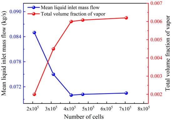
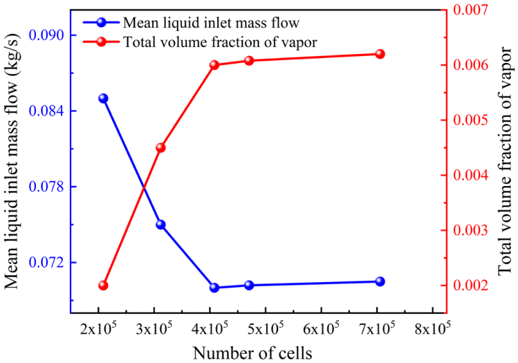
To ensure the reliability of the simulation results, sensitivity analyses for both the computational grid and the time step were performed. First, a grid independence study was carried out using the AVL FIRE code under the operating condition of P_in = 0.3 MPa and P_back = 0.1 MPa. Figure 2 shows the results for five different grid configurations. In this figure, the vapor volume fraction is calculated as the volumetric average over the computational domain of the upper nozzle part, spanning from the nozzle inlet to the nozzle exit plane.

Figure 2. Grid independence study: mean inlet mass flow rate and vapor volume fraction at an inlet pressure of 0.3 MPa.

The results indicated that the grid with approximately 0.4 million cells provided an optimal balance between the computational cost and accuracy for simulating cavitating flow. In this selected configuration, the boundary layer mesh at the nozzle orifice was refined to a size of 0.03 mm, with a maximum grid size of 0.2 mm in the orifice region. The maximum dimensionless wall distance (y⁺) was maintained at approximately 30, ensuring adequate resolution of the near-wall flow.

The standard wall function is employed to bridge the viscous sublayer and the fully turbulent region, as the present near-wall resolution (y⁺ ≈ 30) does not resolve the viscous sublayer directly. This treatment is adequate for the present RANS simulations, which focus on the bulk cavitating flow and global parameters such as the mass flow rate and cavity length.

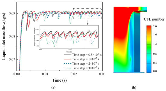
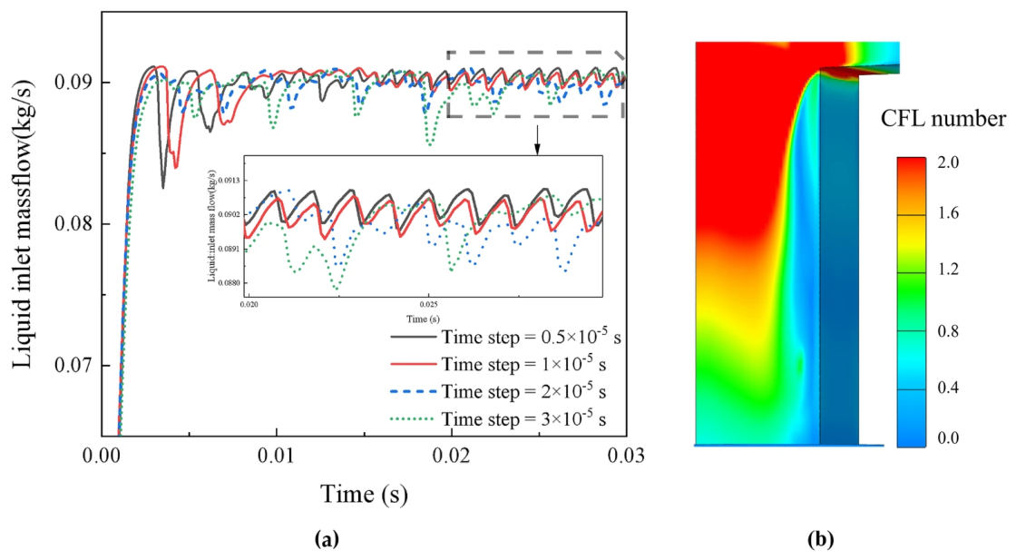
Subsequently, the influence of the calculation time step was investigated to capture the fluctuating cavitation flow accurately. As presented in Figure 3a, the inlet mass flow results for time steps of 3 × 10⁻⁵ and 2 × 10⁻⁵ s differed significantly from the finer time steps. Since the results for 1 × 10⁻⁵ and 0.5 × 10⁻⁵ s showed the same frequency and magnitude of the fluctuations, the larger time step of 1 × 10⁻⁵ s was selected for computational efficiency.

Figure 3. Temporal independence study: (a) inlet mass flow rate under different time step sizes at Pin = 0.35 MPa and (b) Courant–Friedrichs–Lewy (CFL) number distribution on the nozzle wall for a time step of 10⁻⁵ s.

The corresponding Courant–Friedrichs–Lewy (CFL) number distribution is presented in Figure 3b. Along the side wall, the CFL number remains below 1 throughout the entire nozzle length. Along the other walls, the CFL number is close to 2 in the upstream region (from the inlet to approximately half of the orifice length) and drops below 1 from that point to the nozzle exit. In the bulk flow and inlet regions, at some distance from the walls, local CFL values can exceed 2. These elevated values arise from the coarser mesh resolution in those zones. Although the flow velocities in the present simulation are below 35 m/s—lower than the hypothetical > 50 m/s mentioned in typical discussions of CFL stability—the mesh coarsening away from the walls is the primary factor responsible for the localized CFL > 1.

Because an implicit Euler time stepping scheme is employed, the computation remains stable despite the local CFL exceeding unity. It should be noted that in portions of the bulk flow and inlet region, the local CFL number exceeds 2. Under these conditions, the first-order implicit Euler scheme combined with the first-order upwind discretization introduces a non-negligible level of numerical diffusion. This artificial viscosity selectively dampens high-frequency, small-scale pressure fluctuations in those zones; therefore, the high-frequency transient content in the upstream region should be interpreted with caution. Crucially, this concern does not extend to the near-nozzle region—including the near-exit wall and side wall—where cavitation develops and interacts with the boundary layer. In this region the grid is substantially refined, the CFL number remains near or below unity, and numerical diffusion is correspondingly suppressed. The dominant unsteady phenomena analyzed, such as the hydraulic-flip-induced oscillation frequency, are large-scale, low-frequency events that carry significantly more energy than the damped small-scale fluctuations. A dedicated time-step sensitivity study confirmed that further reducing the CFL number does not appreciably change the dominant frequency or the amplitude of mass flow fluctuations. No spurious oscillations or non-physical instabilities are observed in the computational domain. Together with the time-step independence demonstrated in Figure 3a, this confirms that the selected time step of 1 × 10⁻⁵ s provides a suitable balance between temporal accuracy and computational cost.

3.2. Model Validation

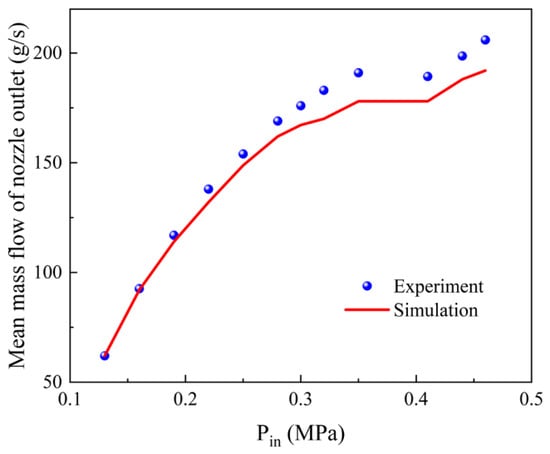
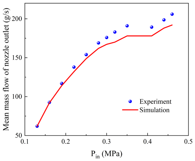
Figure 4 shows that, at a constant back pressure of 0.1 MPa, the simulated time-averaged mass flow rate closely matched the experimental data extracted from Figure 8 of ref. [34] for inlet pressures of 0.13 to 0.46 MPa. Fluctuations occurred when the inlet pressure exceeded 0.2 MPa, indicating cavitation. Significant deviations were noted between 0.25 and 0.35 MPa, with a decline in the growth rate and a collapse between 0.35 and 0.43 MPa.

Figure 4. Validation of the numerical model: comparison of simulated and experimental [34] nozzle outlet mass flow rates across a range of inlet pressures.

The numerical predictions slightly underestimate the experimental values, with a maximum relative error of 6.7% in the 0.35–0.43 MPa range, which corresponds to the transition from sheet cavitation to cloud cavitation (see Figure 5). This deviation is mainly attributable to the assumptions of the Sauer–Schnerr cavitation model, in particular its monodisperse bubble size distribution, which may limit the accuracy in such unsteady transitional regimes. The good overall agreement nevertheless supports the validity of the present model, while the quantitative comparison with the measurements in Figure 8 of ref. [34] confirms its predictive capability.

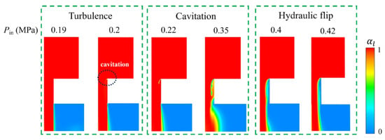
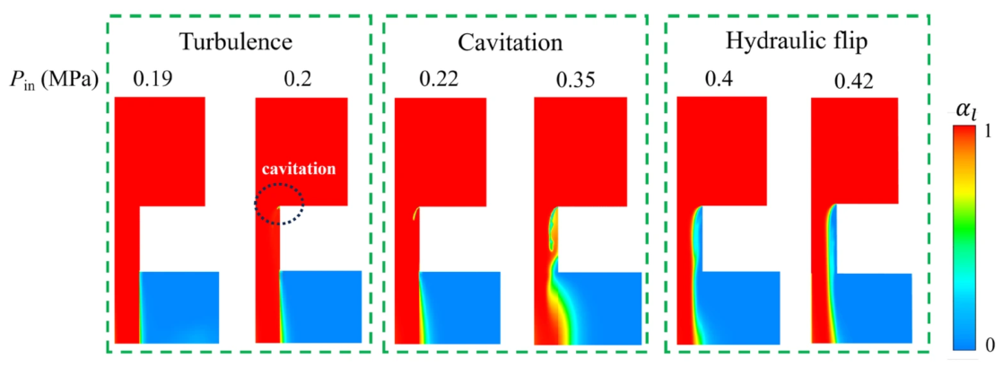
Figure 5. Simulated evolution of the three internal flow regimes (turbulent flow, cavitation flow, and hydraulic flip) in the half-nozzle domain with increasing inlet pressure.

Figure 5 shows the liquid volume fraction contours on the center plane of the computational domain at several inlet pressures, illustrating the three internal flow regimes: turbulent flow, cavitation flow, and hydraulic flip. These regimes correspond to the experimental observations reported in Figure 5a of ref. [34], where high-speed photography was used to capture the flow patterns. These regimes correspond to the experimental observations of ref. [34] (Figure 5a), obtained by high-speed photography. In the experiments, an ellipse marked “cavitation” indicates the inception point; the present simulation captures this inception at a similar location near the inlet corner, and the predicted transition pressures agree closely with the measurements. The model reproduces the progression from cavitation inception to super-cavitation and, finally, to hydraulic flip as the inlet pressure increases. Consistent with the experiments, no cavitation appears under turbulent conditions when the inlet pressure is low (less than twice the back pressure). Sustained cavitation is predicted within a narrow pressure range of 0.25–0.35 MPa. Hydraulic flip occurs once the cavitation region extends to the orifice outlet and covers the entire nozzle length; the gas–liquid interface then remains stable despite further increases in inlet pressure, again in agreement with the observations in ref. [34].

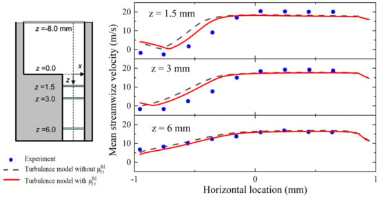
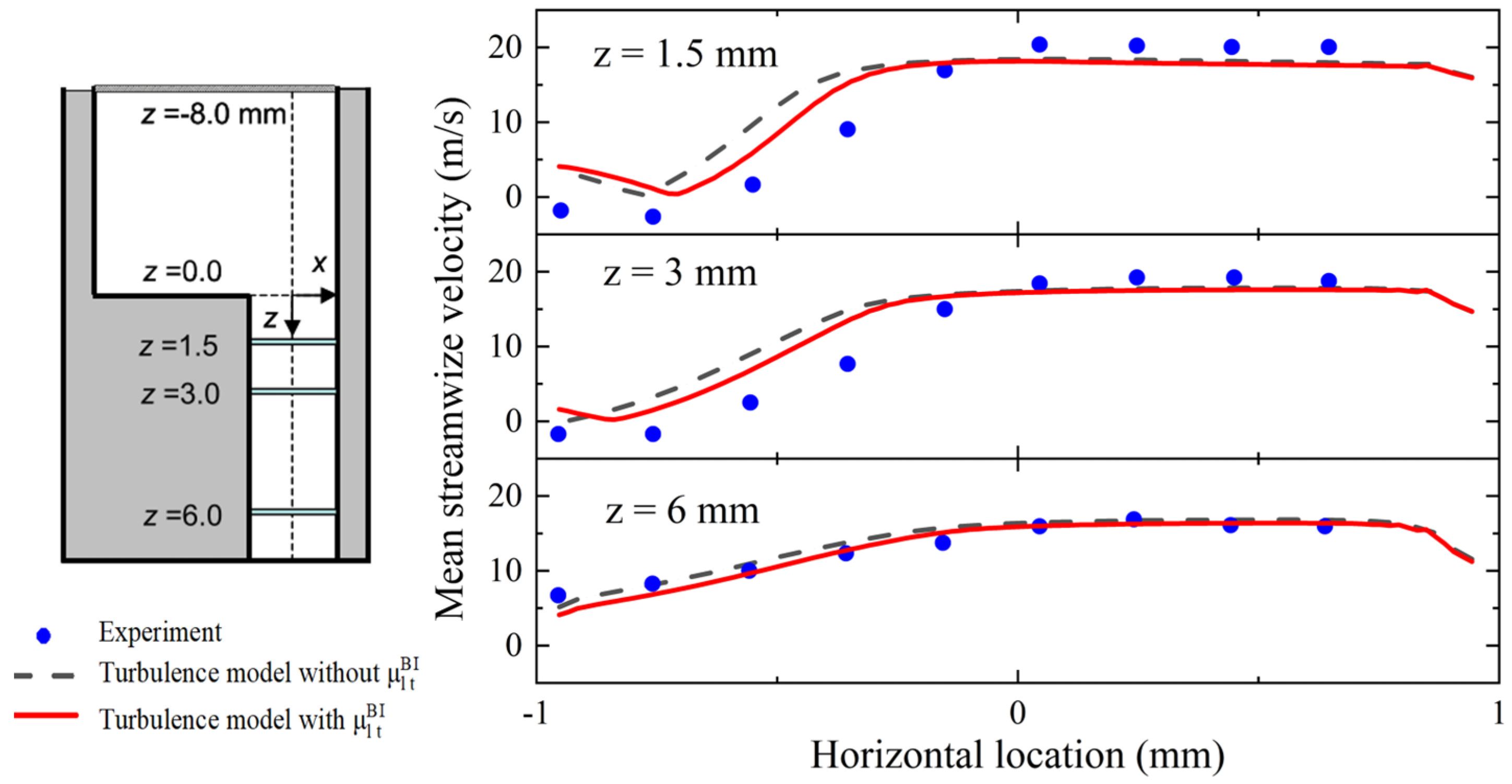
Having validated the baseline model against the flow rate and cavitation regime measurements of ref. [34] (Figure 4 and Figure 5), we further evaluate the bubble-induced viscosity correction using the LDV (laser Doppler velocimetry) velocity data reported by Sou et al. [3] for a different rectangular nozzle geometry (Figure 6). The LDV measurements provide spatially resolved velocity profiles that are not available in ref. [34], thus offering a complementary and more stringent test of the correction model. The correction is introduced via an increased effective viscosity due to the presence of bubbles. A comparison of the mean streamwise velocity at several vertical distances (z = 1.5, 3.0, and 6.0 mm) under an inlet pressure of 0.22 MPa is presented in Figure 6. The results demonstrate that the model with a bubble-induced viscosity (red solid) yielded a marked improvement in accuracy over the baseline model (black dash). The enhancement was particularly evident in the proximal region at z = 1.5 and 3.0 mm, where the simulated velocities with the refined model closely matched the experimental data adjacent to the sidewall. The transient cavitation behavior of the corrected model is examined in the figures in Section 4.1.2; a dedicated spectral comparison with and without the bubble-induced viscosity correction is left for future work.

Figure 6. Comparison of average velocity at different nozzle cross-sections: experimental data (blue dots, extracted and replotted from Figure 6 of ref. [3]), simulation with bubble-induced turbulence modification (red solid), and simulation without bubble-induced viscosity coefficient (black dash).

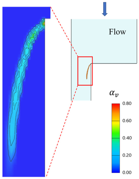
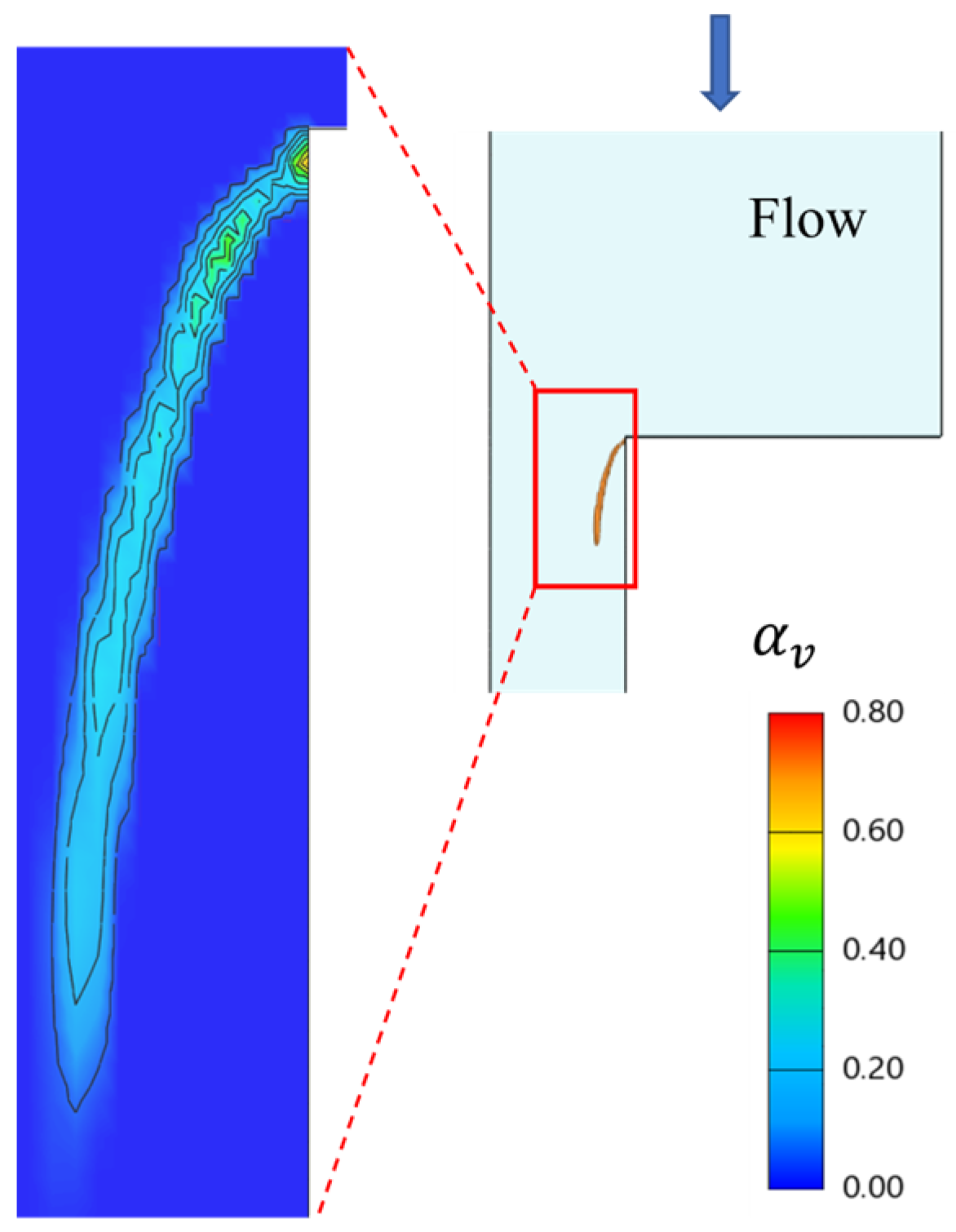
Figure 7 presents the simulated time-averaged vapor volume fraction (void fraction) distribution in the rectangular nozzle at a cavitation number of σ = 7.54, matching the condition of the Venturi-channel experiments reported by Zhang et al. [7]. Their synchrotron X-ray measurements (Figure 10 in ref. [7]) showed that, under developed sheet cavitation, the mean void fraction peaks near the leading edge and decreases sharply towards the solid wall. The present simulation reproduces these key features: the maximum vapor fraction is located close to the cavity leading edge, the fraction drops rapidly to near zero approaching the wall, and the cavitation region remains largely detached from the wall. These qualitative consistencies, despite the geometric differences between the rectangular nozzle and the Venturi channel, support the ability of the numerical model to capture the essential two-phase structure of the cavitating flow.

Figure 7. Simulated time-averaged vapor volume fraction (void fraction) distribution in the rectangular nozzle at a cavitation number of σ = 7.54, the arrow indicates the flow direction, shown for qualitative comparison with the synchrotron X-ray measurements of Zhang et al. [7].

Regarding the discretization scheme used in Section 2.6, the successful validations against the independent experimental data in Figure 4, Figure 5, Figure 6 and Figure 7, covering mass flow rate, regime transitions, velocity profiles, and void fraction, confirm that the numerical diffusion from the first-order upwind scheme does not appreciably affect the predictive accuracy for the key cavitation features. The grid convergence study in Figure 2 further demonstrates that the present mesh resolution is sufficiently fine to constrain the false diffusion to an acceptably low level. Thus, while formally less accurate, the first-order scheme is justified in this strongly unsteady two-phase context without compromising the reliability of the present results.

It is noted that the near-wall resolution yields y⁺ ≈ 30 and the standard wall function is employed. Here, “flow separation” refers to the liquid detaching from the nozzle wall during hydraulic flip (and the associated hydraulic jump), driven by the sharp inlet-edge geometry and the cavitation-induced low pressure—not by a classical adverse pressure gradient. While standard wall functions can delay separation prediction in adverse-pressure-gradient flows, this concern is mitigated for the present case because the separation point is governed primarily by the upstream geometry and the pressure field, rather than by near-wall turbulence details. Consequently, the use of y⁺ ≈ 30 with the standard wall function is not expected to appreciably shift the predicted separation location. This is supported by the good agreement with the experimental data of Park et al. [34] and Sou et al. [3] (mass flow rate, cavitation regime transitions, and velocity profiles; Figure 4, Figure 5 and Figure 6). Resolving the viscous sublayer (y⁺ < 5) with a low-Reynolds-number turbulence model would be required for more precise near-wall flow details and represents a valuable direction for future work.

In conclusion, this analysis demonstrated that the implemented two-fluid Eulerian multiphase model, which incorporated a refined RANS turbulence model and an adjusted S-S cavitation model, accurately captured the cavitation flow transitions and predicted bubble distributions in the nozzles across a wide operating pressure range. The agreement between numerical predictions and experimental data validated the present approach as a reliable tool for the analysis of cavitation dynamics and hydraulic flip phenomena in nozzle flows.

4. Results and Discussion

4.1. Shedding Process in Cavitating Flow

The periodic attachment and detachment of cloud cavitation from the sheet cavity surrounding the orifice wall represents a characteristic quasi-steady state in cavitating flow. In this section, the evolution of the cavity morphology throughout this process is elucidated, the spectral analysis of the shedding frequency is presented, and the mechanisms underlying the shedding are discussed.

4.1.1. Morphology of Cavitation and Length of Cavities

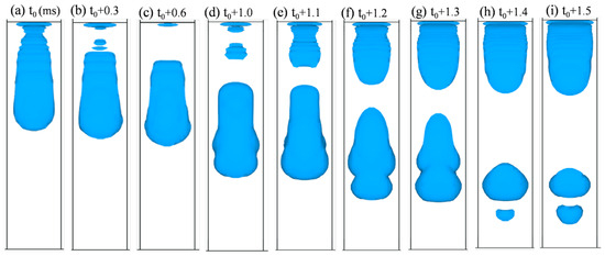
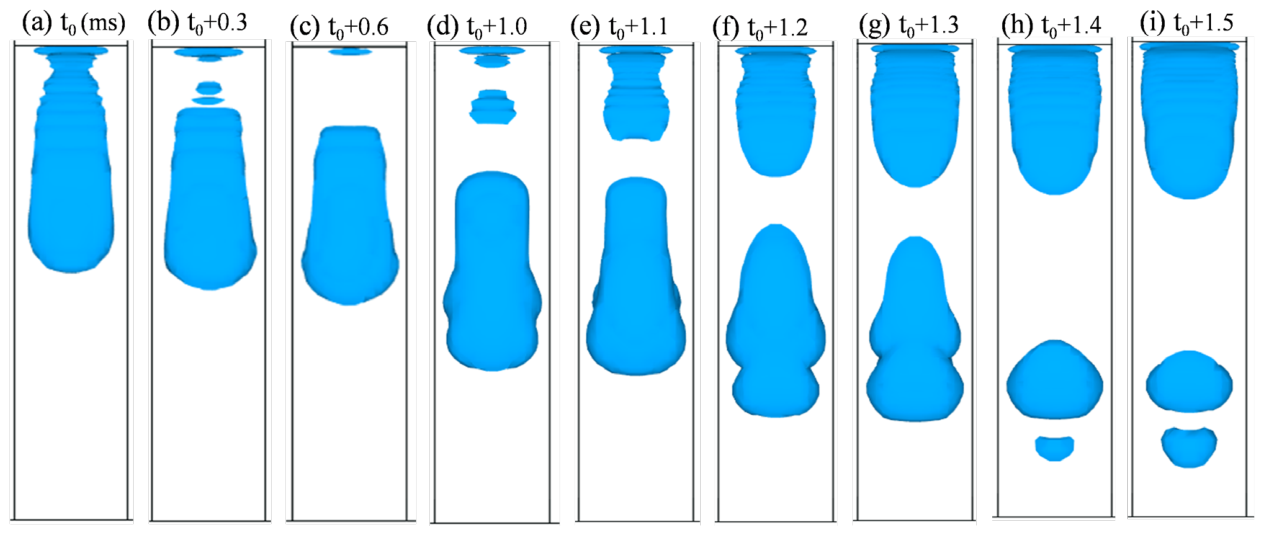
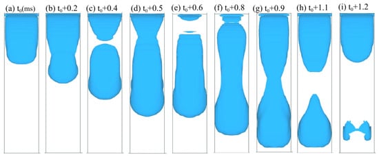
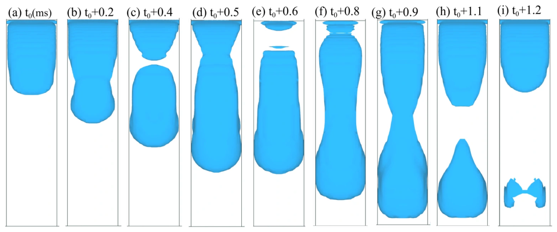
Cavitation near the nozzle wall was categorized into two types: partial cavitation and super-cavitation, which were determined by the length of the cavity. The iso-surface of the vapor volume fraction is utilized to illustrate the morphology of the cavity under varying cavitation conditions, as depicted in Figure 8 and Figure 9. The perspective shown here is a side view of the nozzle, which corresponds to the lateral profile of the side wall presented in Figure 1a.

Figure 8. Morphology of cloud shedding in partial cavitation, P_in = 0.3 MPa (cavitation bubble visualized by the ${\alpha }_v=0.1$ iso-surface, blue).

Figure 9. Morphology of cloud shedding in super-cavitation, P_in = 0.35 MPa (cavitation bubble visualized by the ${\alpha }_v=0.1$ iso-surface, blue).

Figure 8 shows a typical cloud cavitation shedding process at a pressure of Pin = 0.28 MPa. The sheet cavity separated near the inlet edge (Figure 8a–c), while the cavitation cloud progressed downstream as the head shape expanded (Figure 8d–g). This expansion resulted from liquid inertia, which aided bubble accumulation at the cavitation front. Concurrently, a new sheet cavity began to form at the inlet edge and continued to grow until it reached its maximum length (Figure 8c–i). As the cavitation cloud moved downstream, it collapsed rapidly, significantly reducing in size.

Figure 9 shows a typical cycle of sheet growth and cloud shedding under conditions approaching super-cavitation at Pin = 0.35 MPa. The first and second breakages of the sheet cavity near the leading edge, shown in Figure 9c,e, were transient, with the sheet and cloud components reconnecting shortly after (Figure 9f). This process led to a maximum cavitation length nearly equal to the nozzle length (Figure 9g). The actual detachment of the cloud from the sheet cavity occurred following the shrinkage observed in the middle of the sheet cavity (Figure 9h), and the downstream cloud cavity collapsed within the wake flow (Figure 9i).

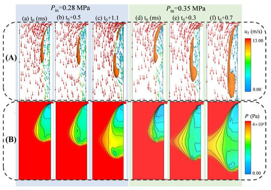
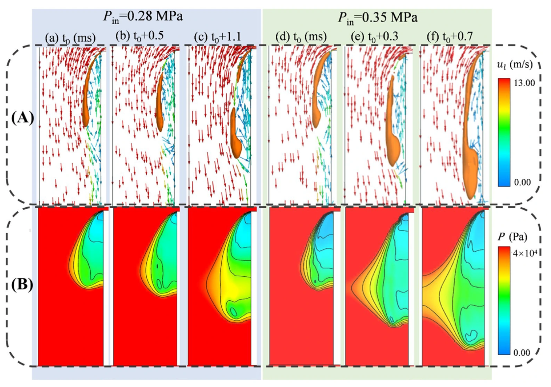
The mechanisms governing cloud cavitation shedding across various regimes have been extensively documented [5,46,47,48]. The classical re-entrant jet mechanism offers a coherent explanation for the morphological differences observed between Figure 8 and Figure 9. To elucidate this mechanism, Figure 10 presents a comparative analysis of the flow fields under two distinct inlet pressures (0.28 and 0.35 MPa), displaying the vapor morphology, liquid velocity vectors, and corresponding pressure distribution.

Figure 10. Comparative analysis of cavitation dynamics and flow fields at P_in = 0.28 and 0.35 MPa: (A) vapor morphology (${\alpha }_v=0.1$ iso-surface, colored orange), with liquid velocity vectors (arrows), and (B) pressure distribution.

At the lower pressure (Pin = 0.28 MPa), the re-entrant jet possessed higher momentum, as evidenced by the faster flow speed in Figure 10A(b). This strong upward backflow effectively disrupted the potential sites for cavity inception, leading to a prolonged stabilization period for the sheet cavity and making its reattachment more difficult, as shown in Figure 10A(c).

In contrast, at the higher pressure (Pin = 0.35 MPa), the cavitation intensity increased, resulting in a larger region of sub-saturation pressure behind the inlet edge and a faster bubble production rate. However, the clustering of larger cloud cavitation bubbles now acted to impede the re-entrant flow near the wall (Figure 10A(e)). Although the reconnection of the separating cavity could form a larger sheet structure (Figure 10B(f)), the subsequent shedding of this cloud was indicated by the migration of the low-pressure core away from the inlet edge. The simulated bubble morphology during this sheet-to-cloud transition is consistent with established experimental observations [5].

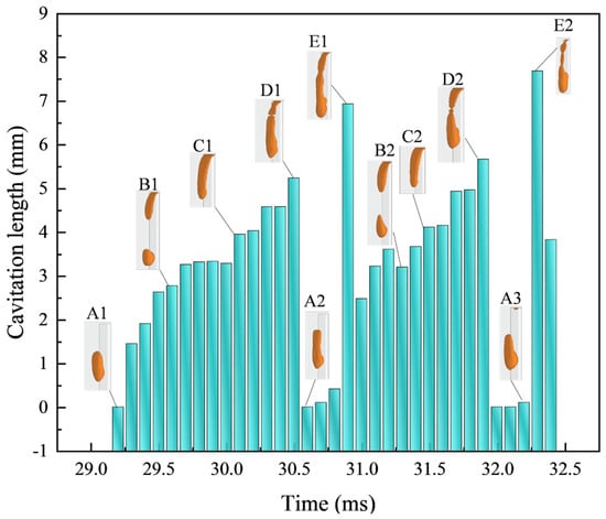
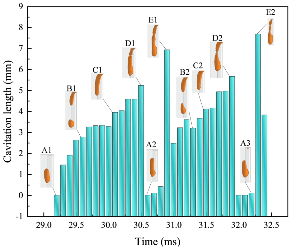
Figure 11 depicts the temporal evolution of the cavitation length over two characteristic cycles (29.3–32.5 ms) at an inlet pressure of 0.3 MPa (partial cavitation regime). To quantify the quasi-periodic development, five distinct states (A–E) were classified based on characteristic lengths, with the morphological patterns in the first cycle (A1–E1) recurring in the next (A2–E2). The sequence from B to D corresponded to the growth stage of the sheet cavity, marked by a continuous increase in length. At the peak length (points D1 and D2), the sheet cavity broke up; its upper section subsequently collapsed (A1 and A3) before reconnecting to form a new cycle (E1 and E2). This figure demonstrated that both the length and morphology effectively characterized the cavitation periodicity.

Figure 11. Variation in cavitation length with time at an inlet pressure of 0.3 MPa (based on the vapor iso-surface at ${\alpha }_v=0.1$, colored orange).

A comparison of the results at 0.28 MPa, 0.35 MPa (Figure 8 and Figure 9), and 0.3 MPa (Figure 11) shows that a higher inlet pressure shifted the sheet cavity detachment point downward, though the shed cloud cavity volume showed little variation. The mean cavity length referenced in the subsequent section corresponded to the point of maximum temporal variation (e.g., from D1 to A2) in Figure 11. At 0.3 MPa, this gave a mean length of 3.39 mm.

4.1.2. Cavity Shedding Frequency and Strouhal Number

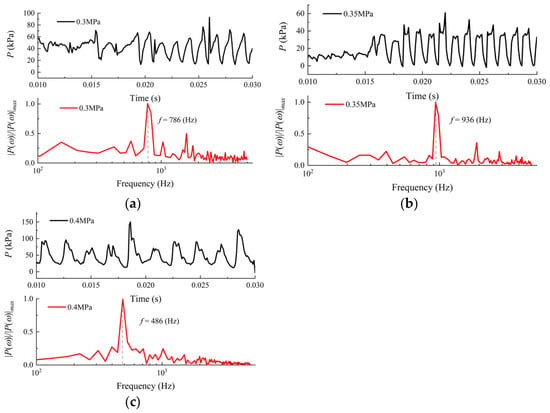
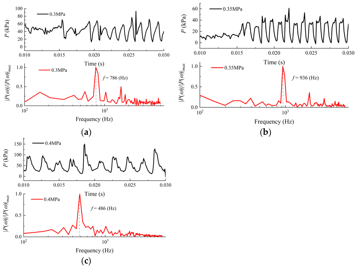
The unsteadiness of the periodic cavitation was characterized by analyzing the time-varying pressure in the flow. The raw pressure signals, spatially averaged over the nozzle orifice, were transformed from the time domain into the frequency domain using a Fast Fourier Transform (FFT). This process revealed the spectral composition of the pressure fluctuations, allowing identification of dominant shedding frequencies along with other harmonic or high-frequency components. Figure 12a,b display three sample pressure traces and their normalized FFT spectra, where P(ω)/P(ω)max denotes the normalized pressure amplitude in the frequency domain for partial cavitation. At the same time, Figure 12c presents the results for super-cavitation. The cloud shedding frequency, derived from these spectra, showed that the dominant frequency for super-cavitation (f = 486 Hz) at Pin = 0.4 MPa was much lower than that for partial cavitation at 0.3 MPa (f = 786 Hz) and 0.35 MPa (f = 936 Hz). This observed decrease in the shedding frequency with increasing cavitation intensity agreed with previous experimental [46,47] and numerical [48] studies.

Figure 12. Temporal evolution of nozzle pressure signal and corresponding normalized fast Fourier transform (FFT) spectrum at (a) Pin = 0.30 MPa, (b) Pin = 0.35 MPa, and (c) Pin = 0.40 MPa.

We further analyzed these oscillations using the Strouhal number, St =$f·l_{cav}/u$, where f is the dominant frequency, $l_{cav}$ is the mean cavity length, and u is the mean streamwise velocity. The estimated Strouhal numbers for various operating conditions are summarized in Table 2. Under periodic shedding conditions, the Strouhal number values range from 0.23 to 0.35, aligning well with the experimental findings of Ganesh et al. [47].

Table 2. Characterizing parameters of the investigated cavitation regimes.

Pin (MPa)	u (m/s)	f (Hz)	${\mathit{l}}_{\mathit{c}\mathit{a}\mathit{v}}$ (mm)	St
0.28	15.9	835	4.3	0.23
0.3	16.6	786	5.32	0.24
0.35	18.1	936	6.7	0.34
0.4	17.6	486	8.8	0.24

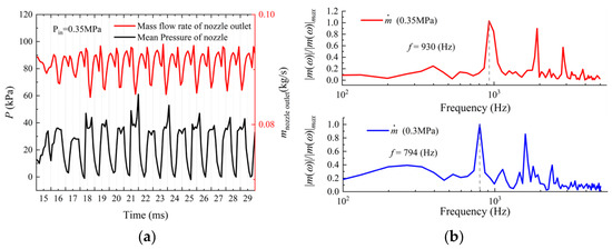
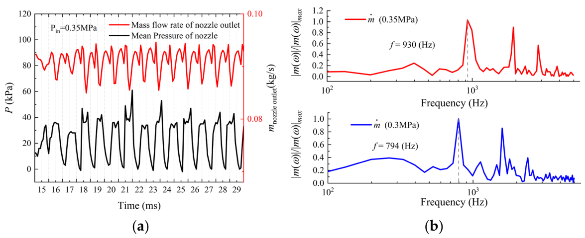
Finally, the phase relationship between the nozzle mass outflow and pressure is shown in Figure 13. Similar to the normalized pressure amplitude P(ω)/P(ω)max presented in Figure 12, m(ω)/m(ω)max denotes the normalized mass flow amplitude in the frequency domain, obtained by scaling the raw amplitude m(ω) with its maximum value. Figure 13a shows that both signals were cyclical but had a half-cycle phase difference, where the mass flow peak aligned with the pressure trough in region A. This relationship was influenced by cloud cavity collapse during shedding, which increased the local pressure and, in turn, accelerated the liquid outflow. The FFT spectra of the mass flow rate in Figure 13b show dominant frequencies of 794 Hz at 0.3 MPa and 930 Hz at 0.35 MPa, which correspond closely to the dominant frequencies found in the pressure spectra of Figure 12. This strong correlation was consistent with the governing flow physics described by Bernoulli’s theorem. At the same time, the observed phase shift was attributed to the local pressure increase caused by the collapse of cavitation bubbles.

Figure 13. (a) Correlation between outlet mass flow and pressure signals, and (b) comparative FFT analysis of mass flow at Pin = 0.35 (upper) and 0.3 MPa (lower).

4.1.3. Turbulent Kinetic Energy and Cavitation Dynamics

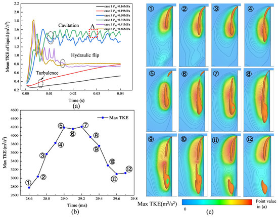
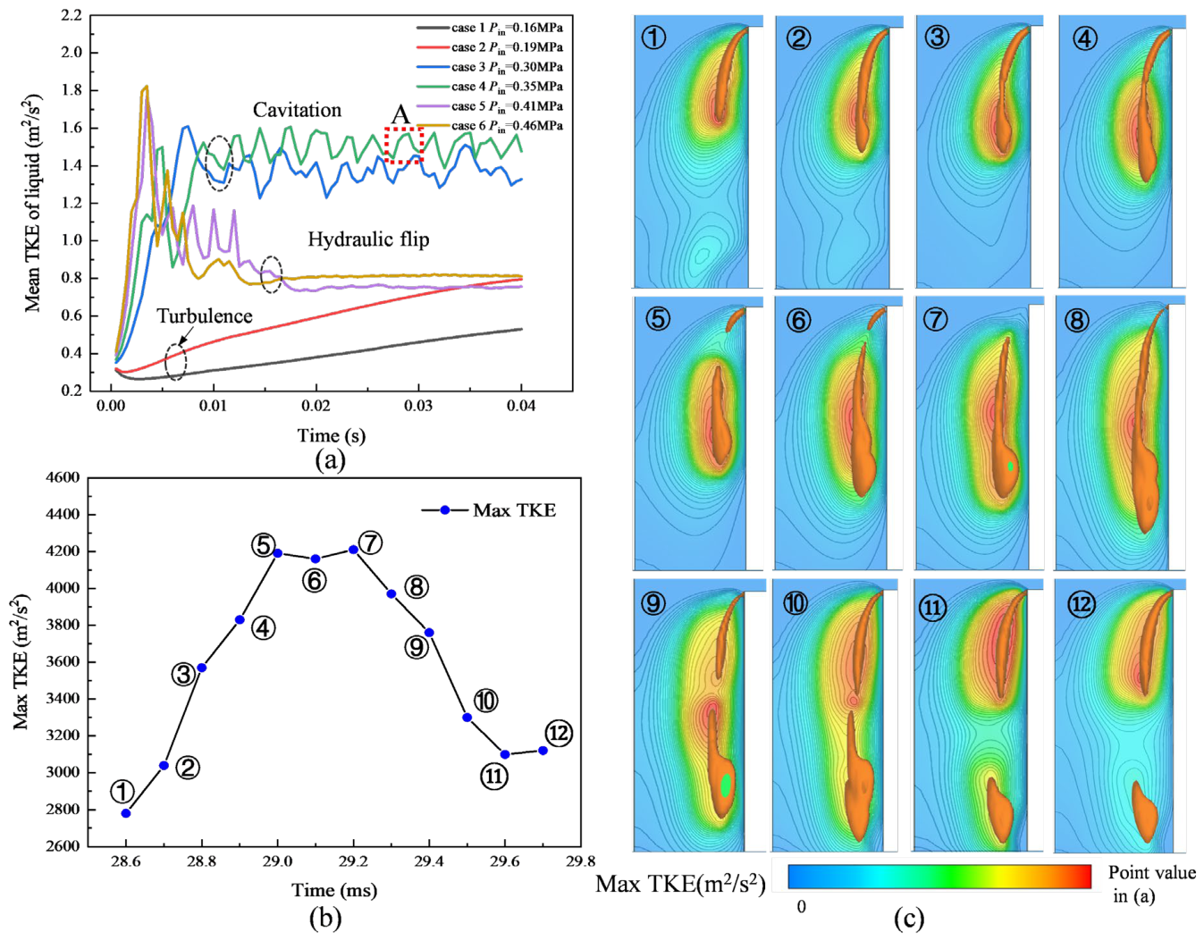
Turbulent kinetic energy (TKE) served as a key indicator of the turbulence intensity in the nozzle flow. As shown in Figure 14a, the mean liquid TKE within the nozzle orifice exhibited distinct trends across the three primary flow regimes. In the cavitating regime, the mean TKE increased rapidly and subsequently fluctuated periodically at a high level. In contrast, during the hydraulic flip regime, it experienced a brief surge before declining and stabilizing at a low value, comparable to the levels observed in the single-phase flow cases (Cases 1 and 2).

Figure 14. Turbulent kinetic energy (TKE) characteristics across flow regimes. (a) Mean TKE trends under cavitating, hydraulic flip, and turbulence conditions. (b) Temporal evolution of the maximum TKE during a cavitation cycle (corresponding to region A in (a)). (c) Instantaneous TKE contours and vapor structures (${\alpha }_v=0.1$ iso-surface) at the time points marked in (b).

The temporal evolution of the maximum TKE in a characteristic cavitation cycle (region A in Figure 14a) is analyzed in Figure 14b. Sequential time points (1 to 12) were selected to represent the key stages of this cycle. The instantaneous flow fields at these specific moments are displayed in Figure 14c, which presents TKE contours overlaid with the vapor iso-surface (${\alpha }_v=0.1$) to correlate the turbulence with the cavitation structure.

The evolution reveals a strong linkage between the TKE and cavity dynamics:

• The cycle initiated at point 1 with the growth of sheet cavitation.
• From points 1 to 5, the maximum TKE rose substantially, driven by the presence of large cavitation bubbles, particularly in the rear section. The TKE value was nearly double its initial level.
• The TKE remained elevated between points 5 and 7, while its peak location shifted from the cavity tail toward its center.
• From points 8 to 10, as the cloud cavitation detached, the location of the maximum TKE stabilized near the detachment area, but its magnitude decreased rapidly.

This spatiotemporal evolution indicates that the growth and convection of the sheet cavitation were the primary mechanisms for amplifying liquid-phase turbulence. Conversely, the detachment and collapse of the cloud cavity influenced the flow predominantly through pressure wave propagation, making a more limited direct contribution to the TKE production.

4.2. Hydraulic Flip

A hydraulic flip occurs when high-speed flow separates from the wall at the nozzle inlet and does not reattach upon exit. In contrast to cavitation flows, hydraulic flip persists over a wider range of working pressures in rectangular nozzles.

4.2.1. Transition from Cavitating Flow to Hydraulic Flip

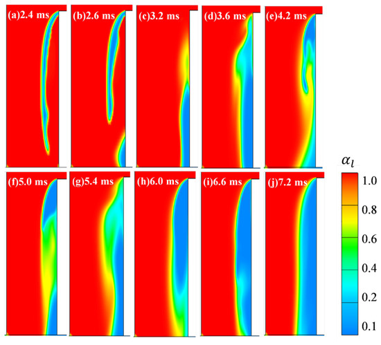
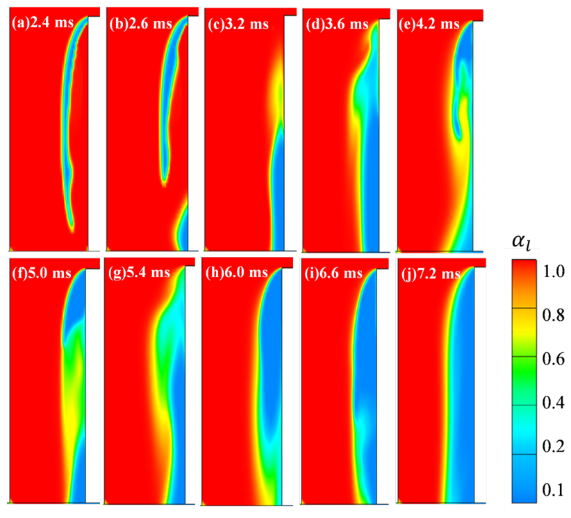
The transition from super-cavitation to hydraulic flip in the nozzle flow is depicted by the evolution of the liquid volume fraction in Figure 15. A large cavity initially spanned most of the nozzle (Figure 15a). It shortened due to cloud shedding, leading to air entrainment (Figure 15b) and a vapor–air mixing process (Figure 15c). Continuous cavitation occurred as high-velocity liquid flowed over the inlet edge, generating vapor bubbles behind the leading edge (Figure 15d,e). The distribution of the liquid and gas phases in the low-pressure cavity region varied significantly (Figure 15f,g) due to re-entrant liquid flow and suction air. Eventually, the main stream moved away from the side wall, forming a hydraulic flip and a clear liquid–gas interface (Figure 15h–j). The nozzle length is crucial for the transition process, which is triggered when the cavitation length approaches the orifice length. Shorter orifices require lower pressures to achieve hydraulic flip, and vice versa.

Figure 15. Transition sequence from super-cavitation to hydraulic flip (Pin = 0.46 MPa).

4.2.2. Transition Time and Flip Thickness

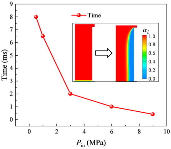
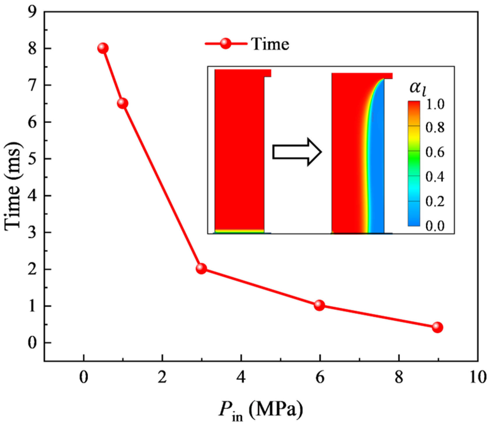
The pressure is essential for a hydraulic flip. Figure 16 shows that the transition time, from start to stable flip, decreased rapidly as the pressure increased from 0.46 to 3 MPa, with only a slight decrease beyond 3 MPa. At 9 MPa, the transition was nearly instantaneous (~0.2 ms). As the pressure increased, the liquid velocity in the nozzle rose, leading to greater inertia. The formation of a hydraulic flip at high pressures was almost immediate, without a discernible transition process.

Figure 16. Hydraulic flip transition time versus inlet pressure (Pin = 0.46, 1, 3, 6, and 9 MPa). The arrow indicates the transition from initial flow to stable hydraulic flip, while the inset shows representative initial and final flip states for all pressures.

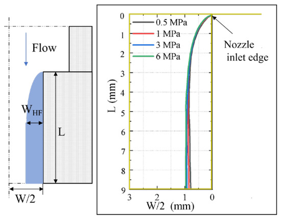
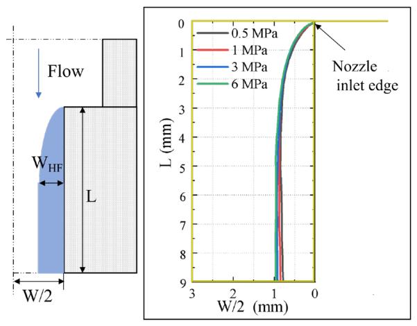
Figure 17 presents the simulated hydraulic flip profiles, identified by regions with a liquid volume fraction exceeding 90%, at injection pressures ranging from 0.5 to 6 MPa. The simulation was performed using the nozzle geometry of ref. [34]. The results indicate that the flip thickness near the inlet remains nearly constant across the investigated pressure range. This insensitivity of the flip thickness to injection pressure is consistent with the experimental trend reported by ref. [31] for a nozzle of different geometry. In that study, the near-constant flip thickness was attributed to the upstream nozzle configuration, which governs the incoming flow angle and limits its variation with pressure. A similar physical mechanism may operate in the present configuration, although the two nozzles differ in geometry, and a direct quantitative comparison is not intended. Consequently, the reduction in the effective flow area yielded a discharge coefficient stably below 1 and remained relatively constant across pressures.

Figure 17. Simulated hydraulic flip profile at various injection pressures, shown by regions with liquid volume fraction above 90%.

4.2.3. Phase Interaction in Non-Liquid Region

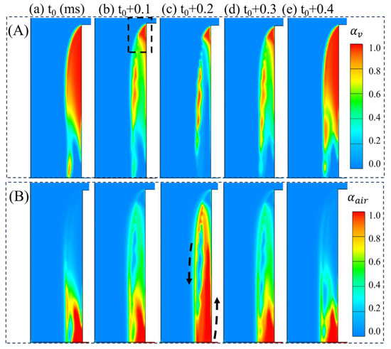
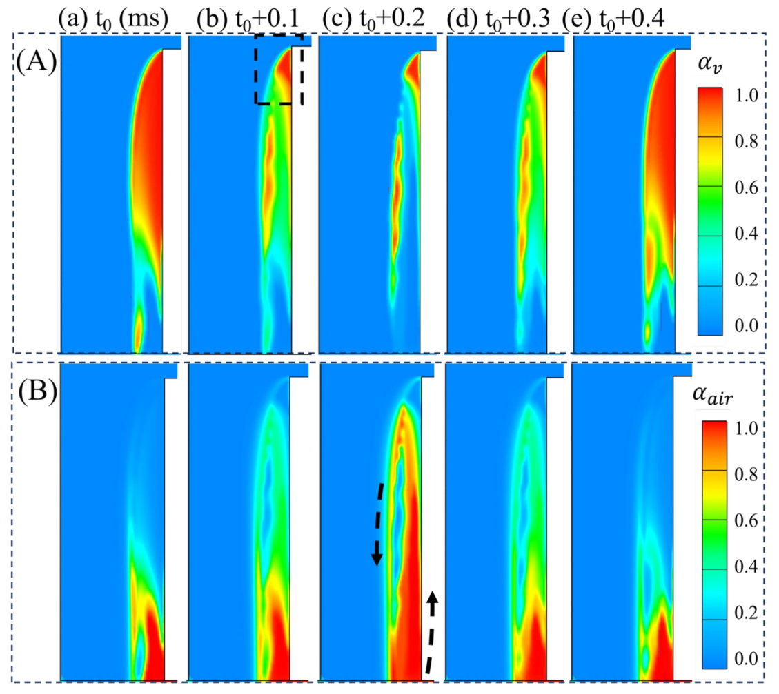
After establishing a stable hydraulic flip, the non-liquid region near the orifice wall contained both vapor and air, as shown in Figure 18. These images show periodic variations in the distributions and volume fractions of these phases. Pure vapor persisted in the triangular area behind the leading edge (black dashed square), where the pressure was always below the saturation point, sustaining a high cavitation intensity. Vapor and air alternately occupied the cavity’s central space. At the outlet, air flowed backward into the orifice, mixing with the vapor and liquid phases as it moved upstream (black arrows). The air distribution area fluctuated periodically, anti-correlated with the vapor phase. This periodic mixing was driven by liquid-phase entrainment. The sustained triangular low-pressure cavitation zone, coupled with a higher ambient air pressure, ensured continuous air inflow and maintained the liquid–wall separation.

Figure 18. Vapor–air interactions in the hydraulic flip non-liquid region (Pin = 6 MPa). (A) Instantaneous vapor volume fraction contours; the black dashed box marks a triangular region that remains pure vapor. (B) Instantaneous air volume fraction contours; black arrows indicate the direction of air motion.

4.2.4. Model Limitations Regarding Bubble Size Distribution and Air Entrainment

Certain limitations of the present modeling approach should be acknowledged, particularly regarding the representation of bubble size dynamics and their influence on air back-suction during hydraulic flip. The Sauer–Schnerr cavitation model adopts a monodisperse assumption, treating all bubbles as having the same radius at a given location. While this simplification is computationally efficient and adequately captures the global cavitation dynamics (e.g., shedding frequency, cavity length), it does not resolve bubble coalescence and breakup, which are known to play significant roles in cloud cavitation and hydraulic flip.

In the context of air back-suction (see Figure 15 and Figure 18), the gas phase in the separated flow region consists of both cavitation-generated vapor and air entrained from the downstream chamber. The mixing and transport of these two components depend on the bubble size distribution, which governs the interfacial area and the momentum exchange between phases. The monodisperse assumption may therefore oversimplify the vapor–air mixing process, particularly when the cavity approaches the nozzle exit and air back-suction intensifies. Accurately capturing the evolution of the bubble size distribution and its effect on interfacial interactions would require a polydisperse model coupled with a population balance approach. Such a refinement lies beyond the scope of the present study but represents a meaningful direction for future work.

It should also be noted that the viscous stress tensor of the gas phase is neglected in the present formulation. While this simplification is reasonable for cavitating flows where the gas phase exists as dispersed bubbles and interfacial forces dominate its momentum balance, it may become less accurate in the hydraulic flip regime, where the gas volume fraction approaches unity in the separated region. In this gas-dominated zone, the gas-phase viscous stress could potentially affect the detailed velocity profile near the gas–liquid interface. Future work employing a full two-fluid model with a complete gas-phase stress closure would be desirable to assess the quantitative impact of this simplification.

5. Conclusions

In this study, the cavitation dynamics and transition mechanisms to hydraulic flip in an internal nozzle were systematically investigated through numerical simulations. The main conclusions are summarized as follows:

(1) Model validation and predictive capability: The Eulerian two-fluid framework was significantly improved through two critical modifications: strategic calibration of the initial bubble number density (10¹⁴ m⁻³) in the cavitation model to capture the inception and transition pressures accurately, and incorporation of the bubble-induced viscosity in the turbulence model to enhance mean flow prediction. It reliably reproduced the quasi-periodic shedding, the decrease in the dominant frequency with rising inlet pressure, and the role of sheet cavitation in enhancing turbulent kinetic energy. The model’s validity was confirmed through strong agreement with experimental LDV and X-ray data in predicting the flow velocity, cavity structures, and Strouhal numbers (0.23–0.35).

(2) Hydraulic flip characteristics: The detailed dynamic pathway from super-cavitation to hydraulic flip, involving a vapor–air mixing process, was elucidated. The transition time to hydraulic flip was strongly dependent on the inlet pressure, becoming nearly instantaneous at high pressures (e.g., 9 MPa). However, once established, the hydraulic flip thickness remained relatively stable across different pressures, as it was likely attributed to the incoming flow angle, which was determined by the upstream nozzle geometry.

(3) Phase interactions in the non-liquid region: Following the stable establishment of the hydraulic flip, periodic vapor–air interactions within the non-liquid region of a stable hydraulic flip were revealed. A pure vapor zone persisted in the triangular low-pressure region behind the inlet edge, while periodic alternation and mixing of vapor and entrained air occurred in the central cavity. This dynamic process was driven by liquid entrainment and the pressure difference between the interior and exterior of the cavity.

In summary, the model developed and the findings obtained in this work enhance the understanding of the underlying physics of the cavitation flow and hydraulic flip in nozzles, providing valuable insights for optimizing spray system design in related power devices.

References

- Huang, B.; Zhao, Y.; Wang, G. Large Eddy Simulation of Turbulent Vortex-Cavitation Interactions in Transient Sheet/Cloud Cavitating Flows. Comput. Fluids 2014, 92, 113–124. [Google Scholar] [CrossRef] [Scilit]
- Danlos, A.; Ravelet, F.; Coutier-Delgosha, O.; Bakir, F. Cavitation Regime Detection through Proper Orthogonal Decomposition: Dynamics Analysis of the Sheet Cavity on a Grooved Convergent-Divergent Nozzle. Int. J. Heat Fluid Flow 2014, 47, 9–20. [Google Scholar] [CrossRef] [Scilit]
- Sou, A.; Biçer, B.; Tomiyama, A. Numerical Simulation of Incipient Cavitation Flow in a Nozzle of Fuel Injector. Comput. Fluids 2014, 103, 42–48. [Google Scholar] [CrossRef] [Scilit]
- Lee, Z.; Kim, T.; Park, S.; Park, S. Review on Spray, Combustion, and Emission Characteristics of Recent Developed Direct-Injection Spark Ignition (DISI) Engine System with Multi-Hole Type Injector. Fuel 2020, 259, 116209. [Google Scholar] [CrossRef] [Scilit]
- Zhang, G.; Zhang, D.; Ge, M.; Petkovšek, M.; Coutier-Delgosha, O. Experimental Investigation of Three Distinct Mechanisms for the Transition from Sheet to Cloud Cavitation. Int. J. Heat Mass Transf. 2022, 197, 123372. [Google Scholar] [CrossRef] [Scilit]
- Zhang, G.; Khlifa, I.; Coutier-Delgosha, O. A Comparative Study of Quasi-Stable Sheet Cavities at Different Stages Based on Fast Synchrotron x-Ray Imaging. Phys. Fluids 2020, 32, 123316. [Google Scholar] [CrossRef] [Scilit]
- Zhang, G.; Khlifa, I.; Fezzaa, K.; Ge, M.; Coutier-Delgosha, O. Experimental Investigation of Internal Two-Phase Flow Structures and Dynamics of Quasi-Stable Sheet Cavitation by Fast Synchrotron x-Ray Imaging. Phys. Fluids 2020, 32, 113310. [Google Scholar] [CrossRef] [Scilit]
- Wang, X.; Li, K.; Su, W. Experimental and Numerical Investigations on Internal Flow Characteristics of Diesel Nozzle under Real Fuel Injection Conditions. Exp. Therm. Fluid Sci. 2012, 42, 204–211. [Google Scholar] [CrossRef] [Scilit]
- Wang, X.; Han, Z.; Su, W. Numerical Study of the Impact on High-Pressure and Evaporating Spray Behavior of Nozzle Cavitation at Typical Diesel Engine Conditions. Int. Commun. Heat Mass Transf. 2017, 81, 175–182. [Google Scholar] [CrossRef] [Scilit]
- Dai, Y.; Zhang, X.; Zhang, G.; Cai, M.; Zhou, C.; Ni, Z. Numerical Analysis of Influence of Cavitation Characteristics in Nozzle Holes of Curved Diesel Engines. Flow Meas. Instrum. 2022, 85, 102172. [Google Scholar] [CrossRef] [Scilit]
- Wu, Z.; Hu, C.; Leng, P.; Zhao, W.; Deng, J.; Li, K.; Li, L. Effect of Nozzle Geometry Features on the Nozzle Internal Flow and Cavitation Characteristics Based on X-Ray Dynamic Imaging. Nucl. Instrum. Methods Phys. Res. Sect. A Accel. Spectrometers Detect. Assoc. Equip. 2024, 1058, 168831. [Google Scholar] [CrossRef] [Scilit]
- Zhu, J.; Zhao, D.; Xu, L.; Zhang, X. Interactions of Vortices, Thermal Effects and Cavitation in Liquid Hydrogen Cavitating Flows. Int. J. Hydrogen Energy 2016, 41, 614–631. [Google Scholar] [CrossRef] [Scilit]
- Mohan, B.; Badra, J.; Sim, J.; Im, H.G. Coupled In-Nozzle Flow and Spray Simulation of Engine Combustion Network Spray-G Injector. Int. J. Engine Res. 2021, 22, 2982–2996. [Google Scholar] [CrossRef] [Scilit]
- Mohamed, M.A.E.A.; Abdel Hameed, H.E.S.; Shaltout, R.E.; El-Salmawy, H.A.A. Prediction of the Impact of Nozzle Geometry on Spray Characteristics. ACS Omega 2021, 6, 6218–6230. [Google Scholar] [CrossRef] [Scilit] [PubMed]
- Ishii, M.; Hibiki, T. Thermo-Fluid Dynamics of Two-Phase Flow; Springer: New York, NY, USA, 2016; Volume 4, ISBN 2013206534. [Google Scholar]
- Budich, B.; Schmidt, S.J.; Adams, N.A. Numerical Simulation and Analysis of Condensation Shocks in Cavitating Flow. J. Fluid Mech. 2018, 838, 759–813. [Google Scholar] [CrossRef] [Scilit]
- Fuster, D. A Review of Models for Bubble Clusters in Cavitating Flows. Flow Turbul. Combust. 2019, 102, 497–536. [Google Scholar] [CrossRef] [Scilit]
- Kumar, A.; Ghobadian, A.; Nouri, J. Numerical Simulation and Experimental Validation of Cavitating Flow in a Multi-Hole Diesel Fuel Injector. Int. J. Engine Res. 2022, 23, 958–973. [Google Scholar] [CrossRef] [Scilit]
- Gu, Y.; Zhang, J.; Yu, S.; Mou, C.; Li, Z.; He, C.; Wu, D.; Mou, J.; Ren, Y. Unsteady Numerical Simulation Method of Hydrofoil Surface Cavitation. Int. J. Mech. Sci. 2022, 228, 107490. [Google Scholar] [CrossRef] [Scilit]
- Rzehak, R.; Krepper, E. CFD Modeling of Bubble-Induced Turbulence. Int. J. Multiph. Flow 2013, 55, 138–155. [Google Scholar] [CrossRef] [Scilit]
- Maniscalco, F.; Buffo, A.; Marchisio, D.; Vanni, M. Numerical Simulation of Bubble Columns: LES Turbulence Model and Interphase Forces Blending Approach. Chem. Eng. Res. Des. 2021, 173, 1–14. [Google Scholar] [CrossRef] [Scilit]
- Colombo, M.; Fairweather, M. Multiphase Turbulence in Bubbly Flows: RANS Simulations. Int. J. Multiph. Flow 2015, 77, 222–243. [Google Scholar] [CrossRef] [Scilit]
- Singhal, A.K.; Athavale, M.M.; Li, H.; Jiang, Y. Mathematical Basis and Validation of the Full Cavitation Model. J. Fluids Eng. Trans. ASME 2002, 124, 617–624. [Google Scholar] [CrossRef] [Scilit]
- Schnerr, G.H.; Sauer, J. Physical and Numerical Modeling of Unsteady. In Proceedings of the 4th International Conference on Multiphase Flow, New Orleans, LA, USA, 1 June–27 May 2001. [Google Scholar]
- Zwart, P.J.; Gerber, A.G.; Belamri, T. A Two-Phase Flow Model for Predicting Cavitation Dynamics. In Proceedings of the 5th International Conference on Numerical Methods in Multiphase Flows, Reykjavik, Iceland, 26–28 June 2004; Volume 152, p. 152. [Google Scholar]
- Zhu, J.; Chen, Y.; Zhao, D.; Zhang, X. Extension of the Schnerr-Sauer Model for Cryogenic Cavitation. Eur. J. Mech. B/Fluids 2015, 52, 1–10. [Google Scholar] [CrossRef] [Scilit]
- Chang, M.; Park, S. Spray Characteristics of Direct Injection Injectors with Different Nozzle Configurations under Flash-Boiling Conditions. Int. J. Heat Mass Transf. 2020, 159, 120104. [Google Scholar] [CrossRef] [Scilit]
- Sou, A.; Maulana, M.I.; Hosokawa, S.; Tomiyama, A. Ligament Formation Induced by Cavitation in a Cylindrical Nozzle. J. Fluid Sci. Technol. 2008, 3, 633–644. [Google Scholar] [CrossRef] [Scilit]
- Sou, A.; Hosokawa, S.; Tomiyama, A. Effects of Cavitation in a Nozzle on Liquid Jet Atomization. Int. J. Heat Mass Transf. 2007, 50, 3575–3582. [Google Scholar] [CrossRef] [Scilit]
- Sou, A.; Maulana, M.I.; Isozaki, K.; Hosokawa, S.; Tomiyama, A. Effects of Nozzle Geometry on Cavitation in Nozzles of Pressure Atomizers. J. Fluid Sci. Technol. 2008, 3, 622–632. [Google Scholar] [CrossRef] [Scilit]
- Pratama, R.H.; Huang, W.; Moon, S.; Wang, J.; Murayama, K.; Taniguchi, H.; Arima, T.; Sasaki, Y.; Arioka, A. Hydraulic Flip in a Gasoline Direct Injection Injector and Its Effect on Injected Spray. Fuel 2022, 310, 122303. [Google Scholar] [CrossRef] [Scilit]
- Xie, W.; Luo, Z.; Wang, H.; Zhou, Y.; Liu, Q.; Zhu, Y. Experimental Investigation on Double Wedge Type-V Shock/Shock Interaction Control Subject to SparkJet Array. Acta Mech. Sin. 2026, 42, 125207. [Google Scholar] [CrossRef] [Scilit]
- Li, B.-R.; Liu, C.-L.; Liu, P.-J.; Zhou, T.-L.; Xu, W.-J.; Wang, L.-Q.; Ye, L. Predictive Analysis of the Overall Cooling Effectiveness for Leading-Edge Showerhead Cooling Based on a Thermal Resistance Network Model with Physical Corrections. Aerosp. Sci. Technol. 2026, 176, 112492. [Google Scholar] [CrossRef] [Scilit]
- Park, S.H.; Suh, H.K.; Lee, C.S. Effect of Cavitating Flow on the Flow and Fuel Atomization Characteristics of Biodiesel and Diesel Fuels. Energy Fuels 2008, 22, 605–613. [Google Scholar] [CrossRef] [Scilit]
- Sato, Y.; Sadatomi, M.; Sekoguchi, K. Momentum and Heat Transfer in Two-Phase Bubble Flow—I. Theory. Int. J. Multiph. Flow 1981, 7, 167–177. [Google Scholar]
- Launder, B.E.; Spalding, D.B. The Numerical Computation of Turbulent Flows. Comput. Methods Appl. Mech. Eng. 1974, 3, 269–289. [Google Scholar] [CrossRef] [Scilit]
- Jones, W.; Launder, B. The Prediction of Laminarization with a Two-Equation Model of Turbulence. Int. J. Heat Mass Transf. 1972, 15, 301–314. [Google Scholar] [CrossRef] [Scilit]
- Guo, G.; He, Z.; Chen, Y.; Wang, Q.; Leng, X.; Sun, S. LES Investigations on Effects of the Residual Bubble on the Single Hole Diesel Injector Jet. Int. J. Heat Mass Transf. 2017, 112, 18–27. [Google Scholar] [CrossRef] [Scilit]
- Guan, W.; He, Z.; Zhang, L.; Guo, G.; Cao, T.; Leng, X. Investigations on Interactions between Vortex Flow and the Induced String Cavitation Characteristics in Real-Size Diesel Tapered-Hole Nozzles. Fuel 2021, 287, 119535. [Google Scholar] [CrossRef] [Scilit]
- He, Z.; Guan, W.; Wang, C.; Guo, G.; Zhang, L.; Gavaises, M. Assessment of Turbulence and Cavitation Models in Prediction of Vortex Induced Cavitating Flow in Fuel Injector Nozzles. Int. J. Multiph. Flow 2022, 157, 104251. [Google Scholar] [CrossRef] [Scilit]
- Tomiyama, A.; Tamai, H.; Zun, I.; Hosokawa, S. Transverse Migration of Single Bubbles in Simple Shear Ows. Chem. Eng. Sci. 2002, 57, 1849–1858. [Google Scholar] [CrossRef] [Scilit]
- Tomiyama, A. Struggle With Computational Bubble Dynamics. Multiph. Sci. Technol. 1998, 10, 369–405. [Google Scholar] [CrossRef] [Scilit]
- Drew, D.; Cheng, L.; Lahey, R.T. The Analysis of Virtual Mass Effects in Two-Phase Flow. Int. J. Multiph. Flow 1979, 5, 233–242. [Google Scholar] [CrossRef] [Scilit]
- Liu, W.; He, Y.; Li, M.; Zhu, H.; Zheng, M. Improving Slurry Flow Predictions in Horizontal Pipes: A Modification to the Burns Turbulent Dispersion Force Model. Ocean Eng. 2026, 343, 123515. [Google Scholar] [CrossRef] [Scilit]
- AVL FIRE, Version 2020 R1. AVL FIRE Theory Guide. AVL: Graz, Austria, 2020.
- Stanley, C.; Barber, T.; Rosengarten, G. Re-Entrant Jet Mechanism for Periodic Cavitation Shedding in a Cylindrical Orifice. Int. J. Heat Fluid Flow 2014, 50, 169–176. [Google Scholar] [CrossRef] [Scilit]
- Ganesh, H.; Makiharju, S.A.; Ceccio, S.L. Bubbly Shock Propagation as a Mechanism for Sheet-to-Cloud Transition of Partial Cavities. J. Fluid Mech. 2016, 802, 37–78. [Google Scholar] [CrossRef] [Scilit]
- Trummler, T.; Schmidt, S.J.; Adams, N.A. Investigation of Condensation Shocks and Re-Entrant Jet Dynamics in a Cavitating Nozzle Flow by Large-Eddy Simulation. Int. J. Multiph. Flow 2020, 125, 103215. [Google Scholar] [CrossRef] [Scilit]
Disclaimer/Publisher’s Note: The statements, opinions and data contained in all publications are solely those of the individual author(s) and contributor(s) and not of MDPI and/or the editor(s). MDPI and/or the editor(s) disclaim responsibility for any injury to people or property resulting from any ideas, methods, instructions or products referred to in the content. |
© 2026 by the authors. Licensee MDPI, Basel, Switzerland. This article is an open access article distributed under the terms and conditions of the Creative Commons Attribution (CC BY) license.