


Abstract
Hydraulic fracturing in naturally fractured rock is governed by complex interactions between fluid flow, rock deformation, fracture propagation, and induced seismicity. In this study, a fully coupled hydro-mechanical framework based on the FDEM is developed to investigate fracture evolution and seismic responses during fluid injection in fractured rock masses. Three representative horizontal stress ratios (R = 1.0, 1.5, and 2.0) were considered to investigate the influence of stress anisotropy on fracture propagation and induced seismicity. The results demonstrate that stress anisotropy exerts a dominant control on fracture propagation patterns, fluid pressure diffusion, and induced seismicity. Under low stress ratios, fracture propagation is diffuse and strongly influenced by pre-existing fractures, whereas higher stress ratios promote localized, directional fracture growth controlled primarily by the stress field. Fluid pressure becomes increasingly concentrated with increasing stress ratio, leading to higher injection pressures and more pronounced pressure fluctuations. The spatial and temporal evolution of mean stress and volumetric strain closely follows that of fluid pressure, indicating that fluid pressurization directly controls effective stress reduction and associated deformation. Seismic analysis reveals a systematic decrease in the Gutenberg–Richter b-value with increasing stress ratio, indicating a transition from distributed micro-fracturing to more coherent fracture reactivation and larger seismic events. Under quasi-steady injection pressure conditions, fracture propagation is found to be episodic and unstable, as evidenced by pronounced positive and negative spikes in the fracture volume change rate and associated pressure fluctuations; these are accompanied by intermittent fracture opening and closure, stress redistribution, and temporary reductions in cumulative seismic moment. These findings provide new insights into the coupled mechanisms governing hydrofracturing-induced seismicity and have important implications for the assessment and mitigation of seismic risks in subsurface engineering applications.
1. Introduction
Hydraulic fracturing is a key technology in subsurface energy engineering and is widely applied in unconventional hydrocarbon production, enhanced geothermal systems, and subsurface fluid injection operations such as carbon capture and storage [1,2,3]. By injecting pressurized fluids into the subsurface, the in situ stress state of the rock mass is perturbed, leading to fracture initiation, propagation, and reactivation of existing discontinuities [4,5,6]. These processes enhance reservoir permeability and connectivity but may also trigger induced seismicity through tensile opening, shear slip, or mixed-mode failure along fractures [7]. Consequently, a comprehensive understanding of the coupled hydro–mechanical processes governing fracture evolution and induced seismicity is essential for optimizing stimulation effectiveness while minimizing seismic risk.
Naturally fractured rock masses exhibit strong structural heterogeneity, where pre-existing fractures significantly influence fluid flow pathways, fracture propagation trajectories, and mechanical responses [8,9,10,11,12,13]. Field observations and laboratory experiments have shown that hydraulic fractures often interact with natural fractures through opening, slipping, arresting, or reactivation, leading to complex fracture networks that deviate from idealized planar geometries [14]. These interactions are strongly controlled by in situ stress conditions, particularly stress anisotropy, which governs fracture orientation, propagation stability, and seismic response.
In situ stress conditions play a fundamental role in controlling fracture–fluid interactions [15,16,17]. In particular, stress anisotropy governs fracture orientation, propagation stability, and the competition between tensile fracture opening and shear reactivation [18,19,20,21]. Under low stress anisotropy, fracture propagation may be diffuse and strongly influenced by natural fracture networks, whereas high stress anisotropy tends to promote localized, stress-aligned fracture growth [22,23,24,25]. Microseismic observations from hydraulic fracturing and fluid injection projects further suggest that stress conditions influence not only fracture geometry but also seismic source characteristics, including event magnitude, spatial clustering, and b-value evolution [26,27,28,29]. Despite these observations, the mechanistic links between stress ratio, fracture propagation behavior, and induced seismicity remain incompletely understood.
Numerical modeling provides a powerful tool for investigating these coupled processes. Continuum-based approaches, such as finite element and finite difference methods, have been widely used to simulate fluid–solid interactions and poroelastic responses at the reservoir scale [30,31,32,33]. While effective for capturing large-scale pressure diffusion and stress redistribution, these methods generally require fracture propagation to be prescribed or approximated, limiting their ability to explicitly represent fracture initiation, growth, and coalescence. Discrete approaches, including discrete element methods, allow explicit representation of fracture mechanics and discontinuous deformation but often rely on simplified hydraulic models or weak coupling between mechanical and fluid processes, restricting their applicability to fully coupled hydraulic fracturing problems [34,35].
The Finite–Discrete Element Method (FDEM) offers a robust alternative by combining continuum mechanics with explicit fracture representation within a unified computational framework [36,37,38,39,40]. FDEM allows fractures to initiate and propagate naturally through the progressive failure of interface elements, while maintaining the ability to simulate stress redistribution and deformation in the surrounding rock matrix [41,42,43]. Well-known FDEM software includes Solidity [44], HOSS [45], Y-Mat [21], Y-GUI [46], Irazu [47,48], and Y-HFDEM [49]. Recent advances in FDEM have further enabled fully coupled hydro–mechanical simulations, incorporating fracture opening, shear slip, mixed-mode failure, and fluid flow within dynamically evolving fracture networks [50]. These developments make FDEM particularly well-suited for investigating the complex interactions between fluid injection, fracture evolution, and induced seismicity in naturally fractured rock masses. Despite these advances, systematic investigations of how in situ stress ratio controls fracture propagation patterns, fluid pressure evolution, and induced seismicity within a unified hydro–mechanical framework remain limited. In particular, the relationship between fracture volume growth and seismic moment release during hydraulic fracturing is not yet fully understood.
A fundamental distinction between explicit and implicit hydro-mechanical coupling strategies lies in how the coupled nonlinear system is solved. Implicit schemes solve the fully coupled governing equations iteratively at each timestep, providing unconditional numerical stability and allowing relatively large timesteps. Implicit schemes solve the fully coupled equations iteratively at each timestep, providing enhanced numerical stability and allowing larger timesteps, but at the expense of substantial computational cost and convergence management. In contrast, explicit staggered schemes exchange information between hydraulic and mechanical solvers without iterative correction, making them particularly effective for capturing rapid fracture propagation, dynamic rupture processes, and associated seismic energy release. Recent advances in explicit coupling include the incorporation of finite-strain elastoplasticity and cohesive-zone models into FDEM frameworks [49], the development of two-phase hydro-mechanical coupling within evolving fracture networks [50], and the simulation of CO2 injection in naturally fractured rock masses using staggered HM coupling [51]. On the implicit side, Liu et al. (2025) developed an implicit hydraulic fracturing formulation for permeable rocks with relaxed timestep constraints [32], while Sharafisafa et al. (2025) proposed a continuum-based jointed rock mass model featuring implicit mechanical updating to improve convergence in quasi-static analyses [52]. Pseudo-connections and LGR methods are aimed at integrating multi-stage hydraulic fracturing in horizontal wells with hydrodynamic simulation as a mandatory part of planning the mining of any shale oil or gas reservoir [53]. These studies collectively demonstrate the inherent trade-off between computational efficiency and numerical robustness. Given the emphasis of the present work on dynamic fracture propagation and induced seismicity, the explicit coupling approach is particularly advantageous due to its ability to directly resolve transient fracture processes and associated seismic energy release.
In this study, a fully coupled hydro–mechanical FDEM framework is employed to systematically investigate fracture propagation and induced seismicity during hydraulic fracturing in naturally fractured rock. A stochastic natural fracture network is explicitly embedded within the numerical model, and fluid injection is simulated under different horizontal stress ratios to explore the role of stress anisotropy. The model captures fracture opening, shear slip, stress redistribution, and fluid pressure evolution within dynamically evolving fracture networks, while induced seismicity is quantified using seismic moment calculations. The specific objectives of this work are to (1) elucidate the effects of stress ratio on fracture propagation patterns and fluid pressure evolution, (2) characterize the spatial and temporal evolution of induced seismicity, and (3) clarify the relationship between fracture volume change and seismic moment release. The results provide new physical insights into injection-induced fracture–seismic coupling and offer practical guidance for seismic risk assessment and management in subsurface energy engineering applications.
The novelty of the present framework include: (1) Explicit incorporation of stochastic DFN-controlled hydraulic fracture propagation under varying stress anisotropy conditions; (2) Integrated analysis of fracture evolution, fluid-pressure diffusion, seismic moment release, and b-value evolution within a unified framework; (3) Quantitative investigation of the coupling relationship between fracture volume variation and induced seismicity; (4) Identification of episodic fracture growth and transient seismic-moment reduction caused by stress redistribution.
2. Mathematical Formulation
2.1. Governing Equation
The mechanical solver is governed by the discretized form of Newton’s second law of motion [38,48,51]:
In this context, represents the lumped mass matrix (kg); denotes the viscous damping matrix (kg/s); and refers to the vector of nodal displacements (m). The vector corresponds to the internal resisting forces (N), including elastic reaction forces and crack-element bonding forces. The vector represents the external forces (N), denotes the contact forces (N), and represents the fluid-pressure forces (N). The equation of motion is integrated at each simulation time step to update the nodal coordinates. This equation ensures equilibrium between the resultant internal forces and other contributing forces.
2.2. Crack Element
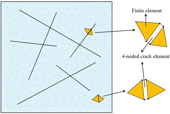
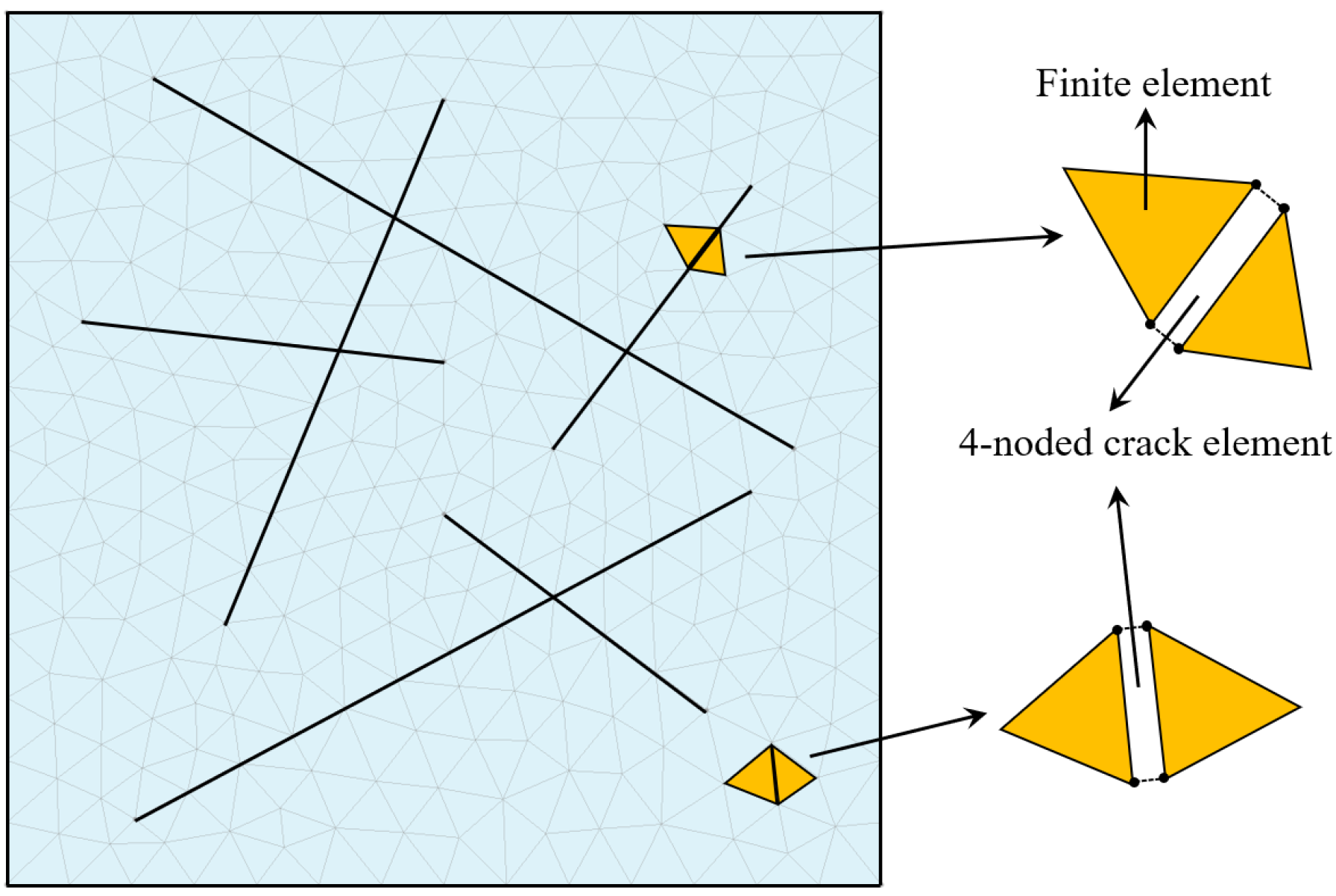
The FDEM analyses conducted in this study begin with discretizing the model domain into constant-strain triangular finite elements. Figure 1 illustrates the discretization of the model domain using constant-strain triangular finite elements and 4-noded interface crack elements. Four-node crack elements are embedded along the interfaces between adjacent finite elements. To explicitly represent natural fractures (NFs), the mesh is constructed such that the edges of the triangular elements are aligned with the prescribed NF traces, enabling the interface crack elements to collectively form continuous natural fracture networks.
Figure 1.
Discretization of the model domain into constant-strain triangular finite elements and crack elements.
2.3. Constitutive Behavior of Fracture
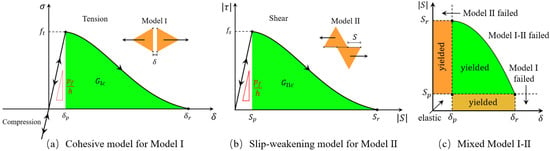
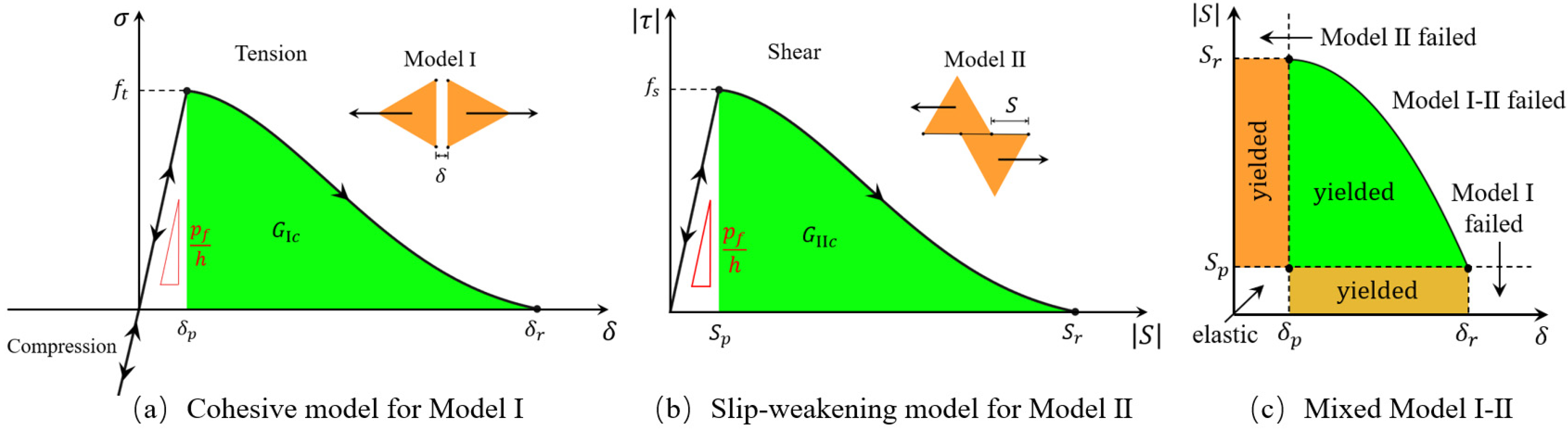
Based on the local stress and the opening of the crack element, crack elements may yield and ultimately fail under Model I (opening), Model II (sliding), or mixed Model I–II loading conditions [48,52], as illustrated in Figure 2.
Figure 2.
Fracture models implemented in FDEM.
For Model I (Figure 2a), the interface behaves elastically at the initial stage. As the crack opening increases from zero, the normal stress increases linearly until it reaches the element tensile strength . The maximum tensile strength point corresponds to the onset of damage initiation at the crack tip and is associated with the proportional opening displacement . Beyond this peak, the material enters a post-peak softening stage, where the cohesive stress progressively decreases with increasing crack opening. This post-peak behavior represents the development of the fracture process zone, during which microcracking and damage accumulation occur while the interface is still able to transfer tensile stress. The tensile stress eventually reduces to zero at the residual opening displacement , indicating complete loss of tensile load-carrying capacity and the formation of a fully open crack, enabling FDEM to capture progressive damage.
In a continuous medium:
When the interface constraint is imposed in penalty function form:
In order for the two approaches to be equivalent, it is necessary that:
In this context, represents the fracture penalty (N/m); denotes the nominal element side length (m); denotes the crack element opening (m); and refers to the penalty stiffness (Pa/m). Dividing the fracture penalty by the element side length introduces a characteristic length scale that converts displacement jumps into equivalent strains, ensuring mesh-size-independent stiffness, energy dissipation, and fracture evolution in the FDEM framework.
According to Figure 2a, the green shaded area under the stress–opening curve corresponds to the Mode I fracture energy , which represents the energy required to create a unit area of new fracture surface in tension. Model I fracture energy governs the post-peak softening behavior and controls the fracture propagation process in the model. can be calculated using the following formula:
For Model II (Figure 2b), at the initial stage, the response is elastic, with shear traction increasing linearly with shear displacement. The slope of this initial stage is controlled by the shear penalty stiffness. The shear strength reaches a peak value at a critical proportional slip displacement . Beyond , the interface enters a post-peak slip-weakening behavior. As sliding continues, the shear traction gradually decreases with increasing slip displacement, representing progressive degradation of shear resistance due to micro-cracking, asperity damage, and frictional weakening. The shear stress eventually reduces to zero at the residual slip displacement , indicating no further shear resistance is provided by cohesion.
The shear strength is usually governed by a frictional strength criterion [47]:
In this context, represents the cohesive strength (Pa); denotes the normal stress acting on the crack faces (Pa); and refers to the material internal friction angle.
According to Figure 2b, the green shaded area under the curve represents the Mode II fracture energy . is the energy dissipated per unit fracture area during shear failure and corresponds to the work done by shear stresses as the crack slips from to .
controls the ductility and energy dissipation capacity of shear fractures in the model. can be calculated using the following formula:
For mixed Model I-II (Figure 2c), the lower-left corner of the diagram corresponds to the elastic regime, where both and , and the crack element behaves elastically. Once either displacement reaches its peak value ( or ), the crack element yields, entering a non-linear softening regime. The yellow region along the horizontal axis (, ) corresponds to pure Mode I yielding, where tensile opening dominates and the crack progressively fails in Mode I. When , the crack element is considered fully failed in Mode I, and no tensile resistance remains. Similarly, the orange region along the vertical axis (, ) represents pure Mode II yielding, dominated by shear sliding. When , the crack element is fully failed in Mode II, with complete loss of shear resistance.
The green curved boundary defines the mixed-mode failure envelope. Stress–displacement states that fall inside this green envelope correspond to mixed Mode I-II yielding, where both opening and sliding contribute to fracture evolution. Once the displacement state reaches this curved boundary, the crack element satisfies the mixed-mode fracture criterion and is considered to have failed under combined Mode I and Mode II loading. The diagram shows that fracture initiation and propagation are not governed by a single displacement component alone, but by the combined effect of normal and shear displacements. The shape of the curved envelope ensures a smooth transition between pure Mode I and pure Mode II failure, reflecting realistic fracture behavior in geomaterials.
2.4. Hydraulic Solver
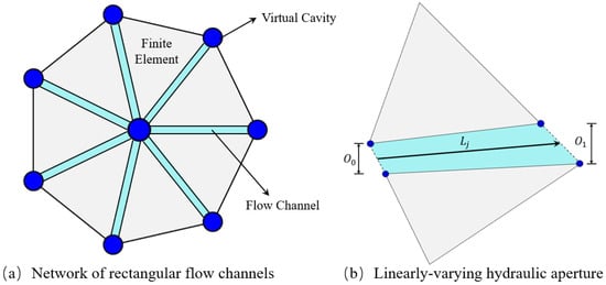
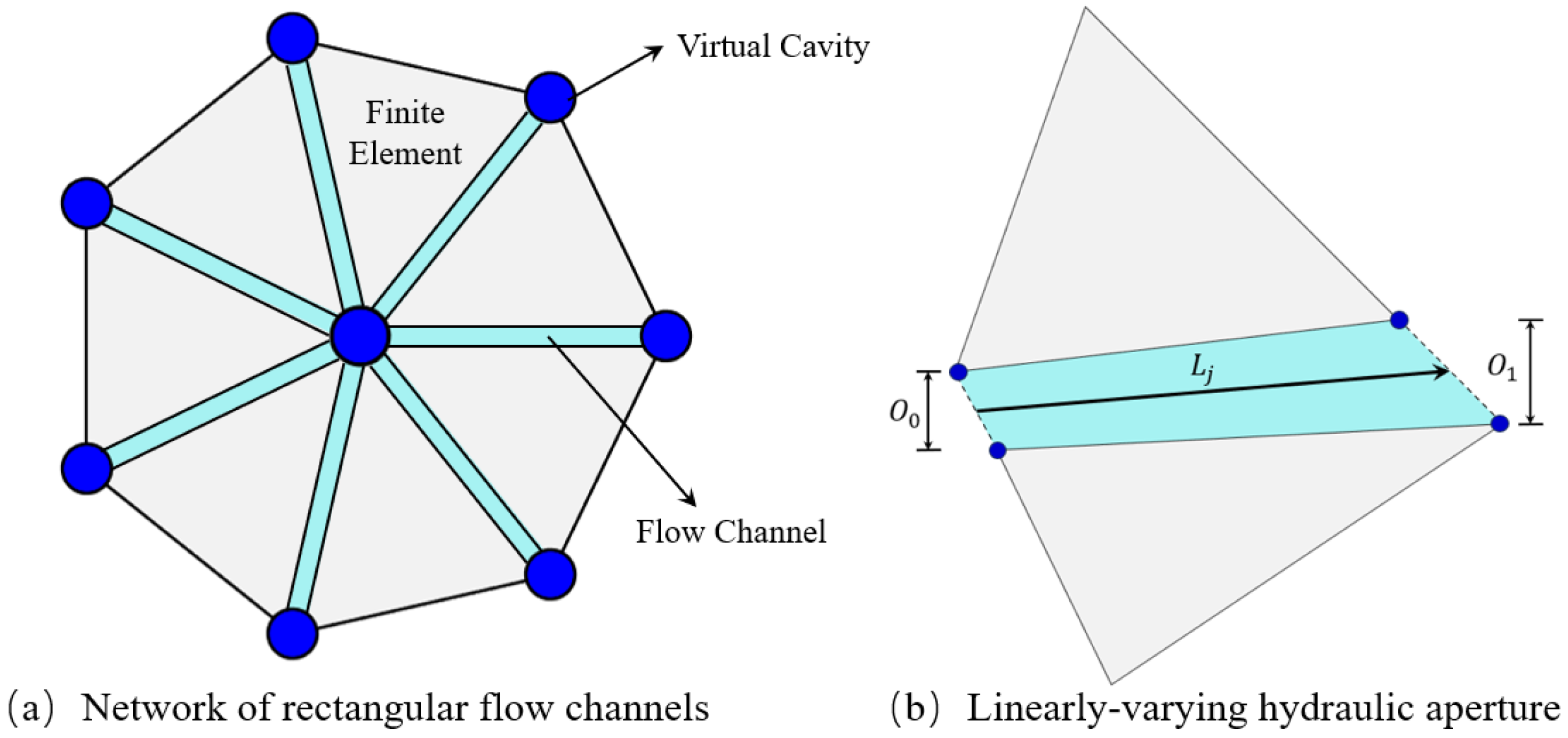
The hydraulic solver is constructed on a channel-cavity network that is directly derived from the triangular finite-element mesh used by the mechanical solver [48], as illustrated in Figure 3. Flow channels are defined along the interfaces between adjacent triangular finite elements. Each channel represents a potential pathway for fluid flow, with its geometry controlled by the deformation of the surrounding solid elements. The length of a flow channel, denoted by in Figure 3b, corresponds to the shared edge between two neighboring triangular elements.
Figure 3.
Computational framework of the finite element–based fluid flow solver.
The volume of the -th flow channel, , is computed as [54]:
In this context, and denote the apertures at the two end points of the channel (m); and refers to the length of a flow channel (m).
The fluid volume stored in a cavity, , is calculated as:
The fluid is assumed to follow a linear compressibility law, meaning that changes in fluid pressure are proportional to changes in fluid density or volume. This assumption is appropriate for slightly compressible fluids. Fluid pressure update during a hydraulic time step is computed as follows:
In this context, and are the fluid pressures at the current and previous time steps, respectively (Pa); is the bulk modulus of the fluid (Pa); is the fluid density (kg·m−3); is the current cavity volume (m3); and refers to the change in fluid mass within a cavity during the hydraulic time step, caused by inflow or outflow through connected flow channels (kg).
If fluid mass increases in the cavity (), the pressure increases. If fluid mass decreases (), the pressure decreases. The pressure increment is larger for stiffer fluids with higher .
Pressure update during mechanical deformation is calculated:
In this context, and are the cavity volumes at the current and previous mechanical steps. This equation accounts for volume changes in the cavity induced by mechanical deformation of the surrounding solid elements.
2.5. Hydro-Mechanical Coupling
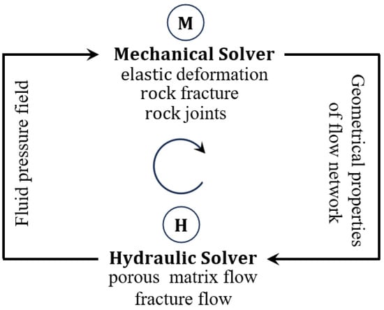
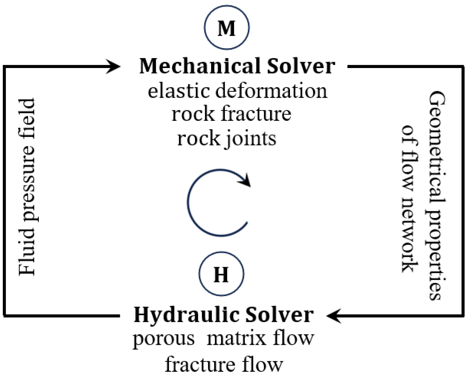
Figure 4 illustrates the two-way, explicit hydro-mechanical (HM) coupling framework, highlighting the interaction between the mechanical solver and the hydraulic solver [48]. The mechanical solver governs deformation and fracture mechanics, altering the geometrical properties of the flow network. The hydraulic solver governs fluid flow and pressure evolution, contributing to effective stress changes, promoting fracture opening, sliding, or reactivation. Information is exchanged bidirectionally at each time step.
Figure 4.
HM coupling strategy in FDEM.
The mechanical timestep is constrained by the Courant–Friedrichs–Lewy (CFL) stability condition for explicit dynamic integration:
In this context, is the P-wave velocity; is the minimum element size; and refers to the stability factor (typically 0.5–0.9 in practice).
The hydraulic timestep is governed by the fluid diffusion stability condition:
In this context, is the hydraulic diffusivity.
2.6. Seismicity Analysis
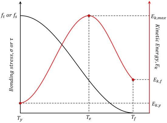
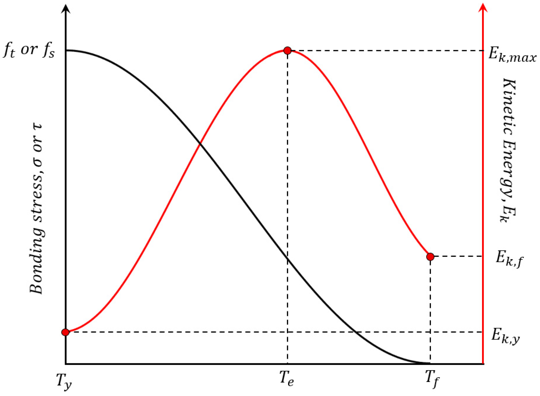
Figure 5 illustrates the temporal evolution of the bonding stress and associated kinetic energy of the crack element. The black curve represents the temporal evolution of the bonding (or shear) stress within a crack element [48]. At , the onset of yielding or damage initiation, the bonding stress remains at a relatively high level, indicating that the crack element is intact and either unbroken or only beginning to be loaded. As external loading increases, the crack element enters a yielding and softening stage. The black curve gradually decreases, reflecting progressive degradation of bonding strength due to damage accumulation and material softening. The bonding stress continues to drop to a very low value or approaches zero at time , indicating that the crack element has lost its load-bearing capacity and that fracture propagation or complete failure has occurred. The black curve demonstrates the mechanical evolution of a crack element from intact → yielding → softening → failure/fracture.
Figure 5.
Temporal evolution of the bonding stress and associated kinetic energy of the crack element.
The red curve shows the temporal evolution of the kinetic energy at the node adjacent to the crack element during crack softening and failure. At , the kinetic energy remains at a low baseline level, implying minimal kinetic energy at the onset of damage. Between and , as the crack element undergoes softening and approaches instability, elastic strain energy stored in the system is progressively released, leading to a rapid increase in nodal kinetic energy. At the critical time , kinetic energy reaches its maximum value, . This peak corresponds to a dynamic rupture event, analogous to the instantaneous energy release during a seismic event. During the post-failure stage, the kinetic energy decays with time due to damping and wave radiation, eventually reaching a lower residual value at time , indicating the system has largely stabilized.
The seismic energy associated with a single crack breakage is assumed to be equal to the maximum value of this kinetic energy increment attained during the crack evolution process. corresponds to the peak kinetic energy generated between the onset of yielding and the final rupture of the crack element. can be calculated using the following formula:
The seismic moment contribution of an individual crack or damage element represents the static strength of the source, and is commonly defined as [55]:
In this context, denotes the shear modulus of the medium (Pa); refers to the slip area of the element (m2); and refers to the slip or opening displacement (m).
represents the characteristic displacement of the -th crack element, defined according to the dominant failure mode as follows. For Mode I-dominated failure (, ), is the tensile opening displacement at the point of complete failure. For Mode II-dominated failure (, ), is the magnitude of the shear slip displacement at the point of complete failure. For mixed Mode I–II failure, is the resultant displacement magnitude, combining both opening and sliding components.
The total seismic moment of an event is:
In this context, is the number of damages belonging to the same seismic event; and refers to the seismic moment (Nm).
A widely used empirical relationship for estimating the moment magnitude is given by [56,57]:
3. Model Setup
The natural fracture network is generated using a stochastic discrete fracture network (DFN) approach. Fracture trace lengths follow a power-law distribution:
with exponent , minimum trace length , and maximum trace length . Fracture orientations follow a Fisher distribution centered at two dominant sets: Set 1 at 45° and Set 2 at 135° (measured from the horizontal). Structural weakening and instability in fractured rock masses govern the evolution of both fluid migration pathways and the loci of mechanical failure [58].
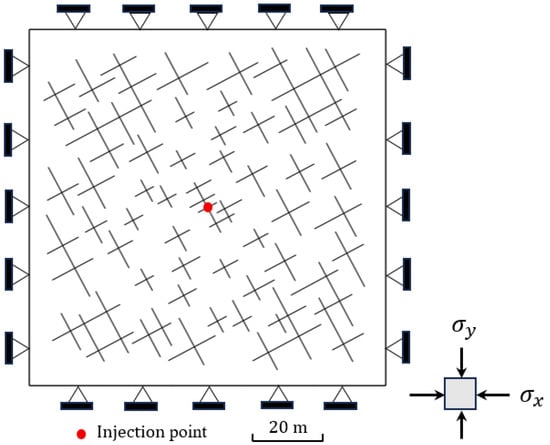
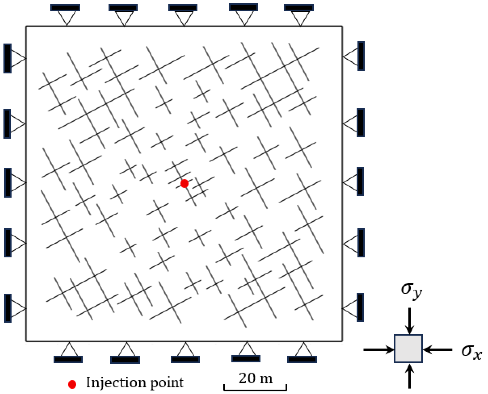
A random natural fracture network is embedded in a square rock domain. Figure 6 demonstrates the model geometry and boundary conditions of the natural fracture network used in numerical simulations. The size of the 2D square fractured rock domain is 100 m, and the red dot at the center of the domain marks the fluid injection point. The injection point is usually chosen away from the boundaries to minimize boundary effects and to observe fracture activation and pressure diffusion under quasi-infinite conditions. The boundaries are subjected to in situ stresses, and displacement constraints are applied around the boundary to prevent rigid-body motion while allowing stress-controlled deformation.
Figure 6.
Geometry and boundary conditions of natural fracture networks.
Two steps are performed in the hydraulic simulation. In the first stage, the system is brought to an initial equilibrium state under in situ stress conditions. In the second stage, the rock mass is modeled by injecting water at a prescribed flow (mass) rate of 0.05 kg/s for up to 2800 s. The rock domain is subjected to an orthogonal in situ stress field, with a minimum horizontal stress of Pa applied along the -direction and a maximum horizontal stress of Pa (Pa, Pa) applied along the -direction.
To quantify the effect of in situ stress on hydraulic fracturing, the stress ratio is introduced:
Stress field inversion is employed to determine the in situ stress state and mechanical properties of deep rock masses [59]. The key material parameters governing the regimes of models in this study are listed in Table 1.
Table 1.
Material parameters for the hydrofracturing.
4. Analysis and Discussion
The numerical results are analyzed in terms of fracture geometry, pressure distribution, stress and strain evolution, and seismic response under different stress ratios (R = 1, 2, 3). Particular attention is given to the interplay between fracture deformation and seismic energy release, aiming to clarify the mechanisms governing episodic fracture growth, stress redistribution, and seismicity behavior during hydraulic fracturing. The following sections discuss these results in detail.
4.1. Fracture Propagation and Fluid Pressure
Figure 2 illustrates the fracture propagation characteristics under different stress ratios at the same simulation time (Time = 2800 s). Blue short line segments represent the pre-existing DFN in the rock mass. These fractures are randomly distributed and oriented, forming the initial structural framework. Magenta (pink) curves indicate newly generated hydraulic fractures or fracture propagation paths induced during hydrofracturing.
The stress ratio R = 1 implies an approximately isotropic horizontal stress state. Fracture propagation shows a radial and dispersed pattern around the injection point. Multiple fracture branches develop in different directions, strongly influenced by nearby pre-existing fractures. This indicates that when stresses are nearly equal, fracture growth is less directionally constrained and more controlled by local heterogeneity.
With an increased stress ratio (R = 1.5), fracture propagation becomes more directionally focused. The hydraulic fractures preferentially propagate along a dominant vertical direction, which corresponds to the orientation perpendicular to the minimum principal stress. In comparison with Figure 2a, the fractures in Figure 2b appear more planar and better aligned.
Under the condition of a higher stress ratio (R = 2), the pronounced stress anisotropy gives rise to increased fracture generation during hydrofracturing. The influence of pre-existing fractures is further weakened, and most new fractures propagate along the maximum principal stress direction. This demonstrates that under a strong stress ratio, fracture propagation is primarily controlled by the in situ stress field rather than by structural heterogeneity.
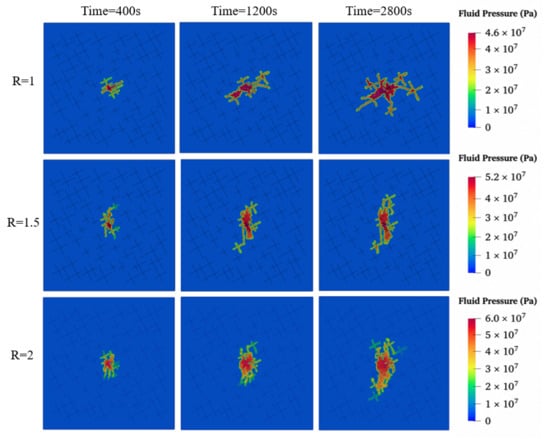
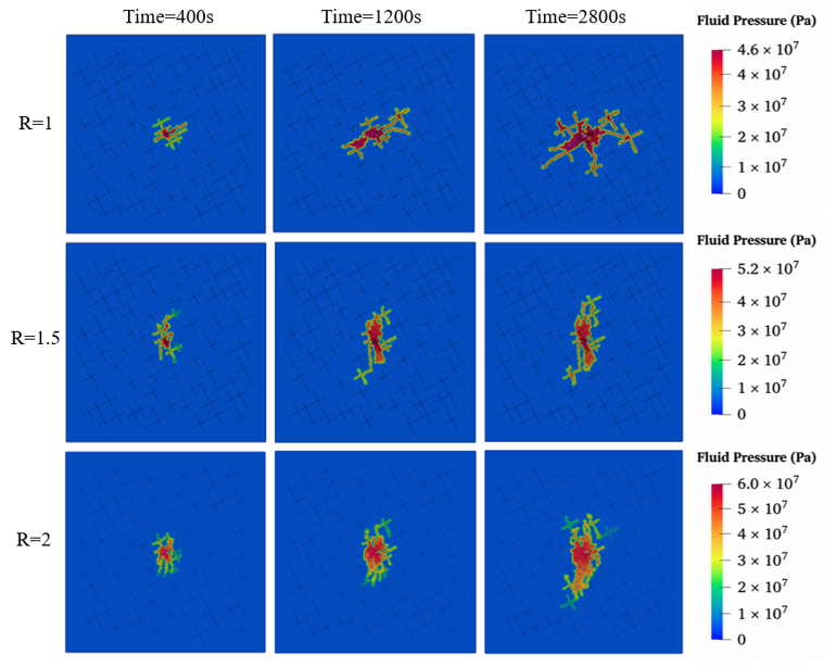
Figure 7 presents the spatial evolution of fluid pressure at three representative time steps under the same stress ratios. For the lower stress ratio (R = 1), high fluid pressure is initially concentrated near the injection point at the early stage (400 s). As injection continues, the pressurized zone progressively expands along multiple fracture pathways. By 2800 s, a broadly distributed high-pressure region has developed, which is consistent with the complex and branching fracture network observed in Figure 2a. For R = 1.5, fluid pressure propagation becomes more elongated and directionally constrained. The pressurized zone expands steadily along the dominant fracture orientation, reflecting the increasing influence of stress anisotropy on fracture growth. The peak pressure reaches approximately 5.2 × 10⁷ Pa, which is higher than that observed for R = 1, indicating stronger resistance to fracture opening and propagation. For R = 2, fluid pressure remains highly concentrated within the main fracture corridor throughout the injection process. The highest peak pressure (approximately 6.0 × 10⁷ Pa) is observed, which is consistent with the strongly confined and localized fracture geometry shown in Figure 2c.
Figure 7.
Fluid pressure evolution during hydraulic fracturing.
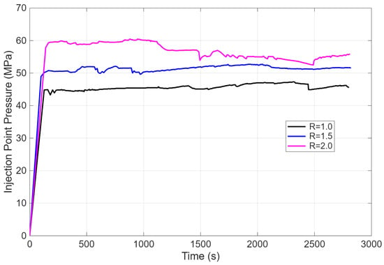
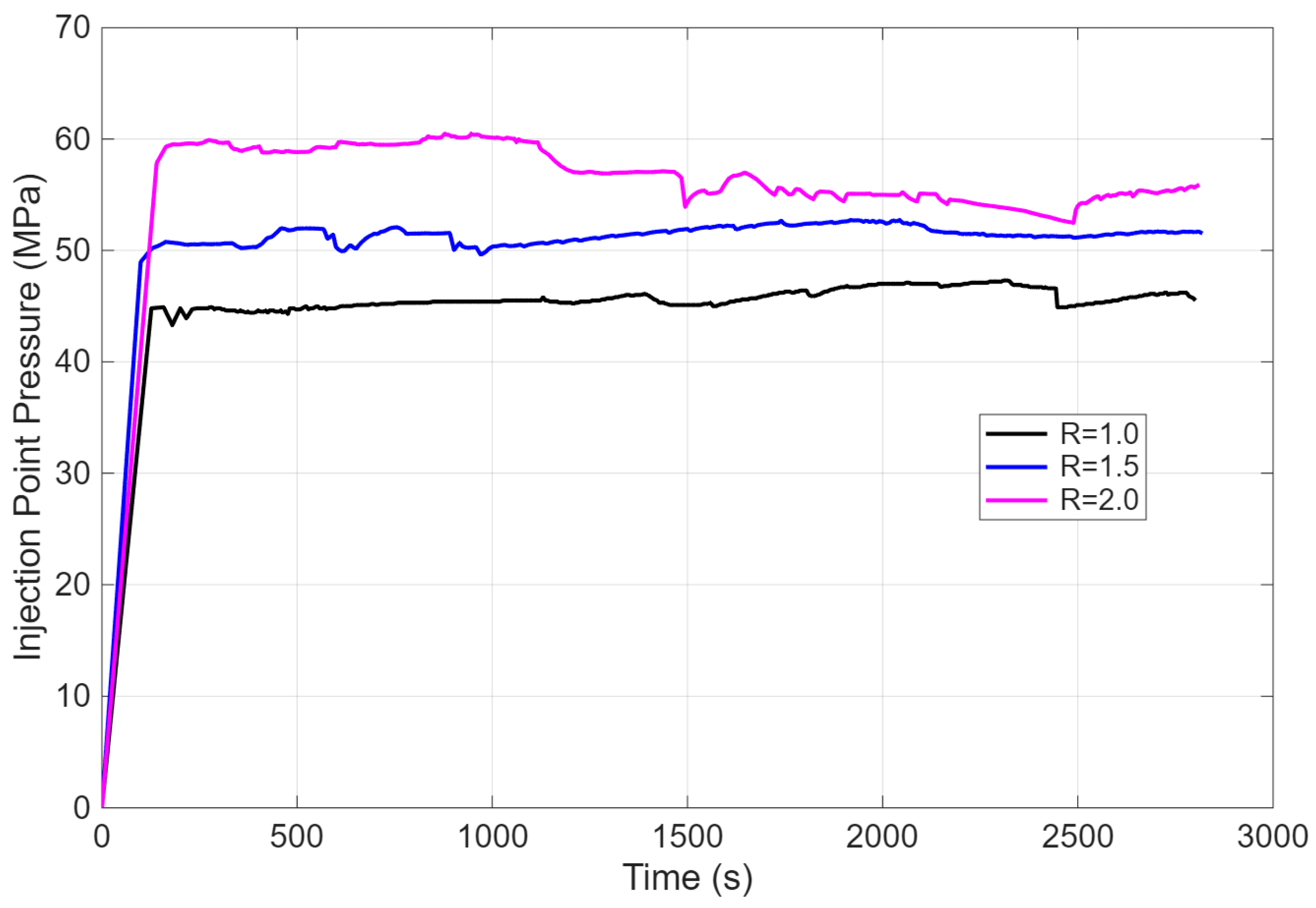
Figure 8 presents the time evolution of injection point pressure during hydraulic fracturing under different in situ stress ratios. All three curves exhibit a rapid and steep rise in pressure immediately after the onset of injection, reflecting fluid filling of the wellbore and nearby fractures prior to significant fracture propagation. As the stress ratio increases, the injection fluid pressure becomes higher, indicating greater resistance to fracture opening under more anisotropic stress conditions. For lower stress ratios (R = 1 or 1.5), the injection pressure curves are relatively smooth and stable, with only minor fluctuations, suggesting gradual fracture opening and steady fluid accommodation. In contrast, under the higher stress ratio (R = 2), the pressure curve shows the largest fluctuations, including pronounced pressure drops. These sudden decreases correspond to abrupt fracture breakthroughs, followed by pressure recovery as fracture propagation continues.
Figure 8.
Injection point pressure under different stress ratios.
4.2. Mean Stress and Volumetric Strain
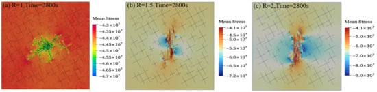
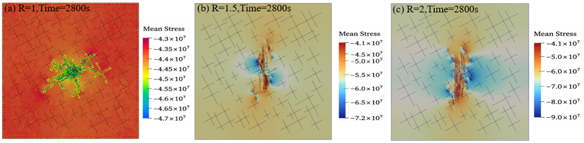
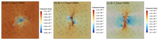
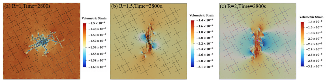
Calculating mean stress plays a crucial role in capturing stress evolution under fluid–rock coupling. It provides a mechanistic basis for understanding damage localization and fracture network development. Figure 9 illustrates the evolution of mean stress during hydraulic fracturing under different in situ stress ratios. Figure 10 shows the corresponding evolution of volumetric strain during hydraulic fracturing under different stress ratios. Fluid injection increases pore pressure, thereby reducing the effective mean stress, which promotes rock dilation and damage accumulation. The negative value represents the compressive state. Negative volumetric strain indicates dilation, typically caused by fracture opening and damage. High mean stress suppresses fracture initiation and propagation by increasing the confining stress, making tensile failure less likely. Low mean stress facilitates fracture initiation, propagation, and interconnection, promoting the development of complex fracture networks. For the isotropic stress ratio (R = 1), a relatively diffuse stress reduction region is observed, coinciding with the complex, branched fracture network. As the stress ratio increases, the mean stress and volumetric strain become higher. For R = 2, a narrow, vertically oriented low–mean-stress zone dominates the domain. Volumetric strain is highly localized and reaches the largest magnitude among all cases.
Figure 9.
Mean stress evolution during hydraulic fracturing under different stress ratios.
Figure 10.
Volumetric strain evolution during hydraulic fracturing under different stress ratios.
4.3. Seismicity
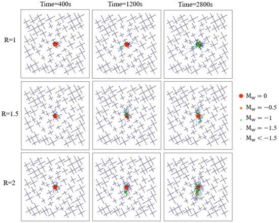
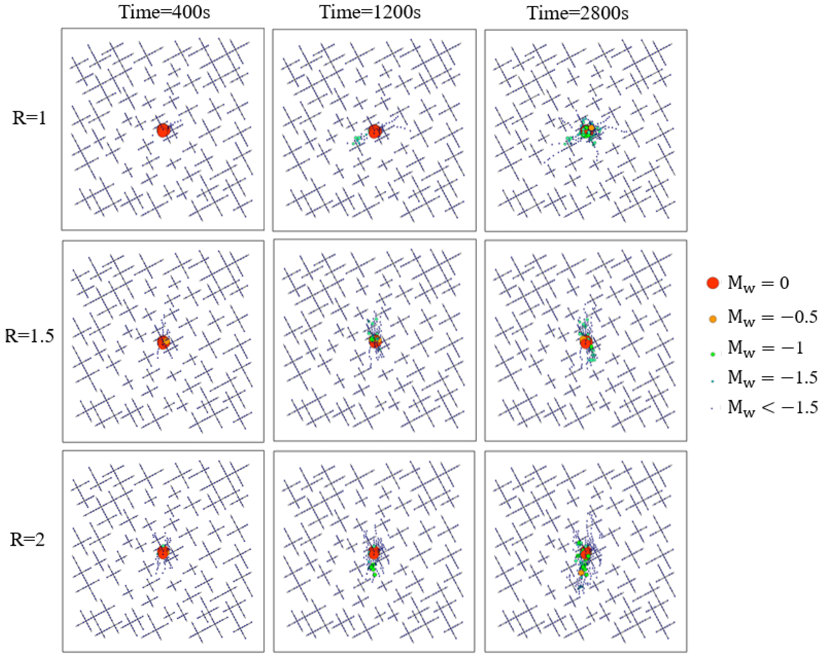
Figure 11 illustrates the spatial distribution and temporal evolution of induced seismic events under different stress ratios. At the early stage (t = 400 s), seismic events for all stress ratios are highly localized near the injection point, forming a compact cluster. Most events exhibit relatively larger magnitudes (Mw ≈ 0 to −0.5), represented by red and orange dots. At this stage, the influence of stress ratio is limited because pore pressure perturbations remain confined to the vicinity of the injection zone. At the intermediate stage (t = 1200 s), seismicity begins to spread along dominant fracture-propagation pathways. Smaller-magnitude events (Mw ≤ −1) become increasingly frequent, particularly for R = 1.5 and R = 2. Compared with R = 1, higher stress ratios show a more elongated and anisotropic seismic cloud, indicating stronger stress control on fracture reactivation. At the late stage (t = 2800 s), seismic events become clearly aligned with pre-existing fracture networks, indicating a higher likelihood of widespread fracture reactivation.
Figure 11.
Spatial distribution and evolution of induced seismic events under different stress ratios.
The seismic moment contributions of each element are listed in Table 2.
Table 2.
Seismic moment contribution of each element.
These results reveal a consistent and clear pattern: although Mode I-dominated fracture elements constitute the majority of failed elements across all stress ratios (58–62%), they contribute only 18–22% of the total seismic moment. The shear-dominated and mixed-mode elements, despite being fewer in number, account for 78–82% of the cumulative M0. This quantitative decomposition provides direct source-mechanical evidence for the decoupling: the large volumetric growth driven by tensile fracture opening generates relatively little seismic moment, while the smaller but mechanically more energetic shear slip events dominate the seismic catalog.
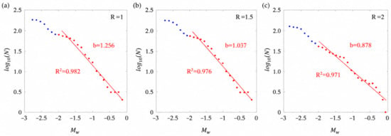
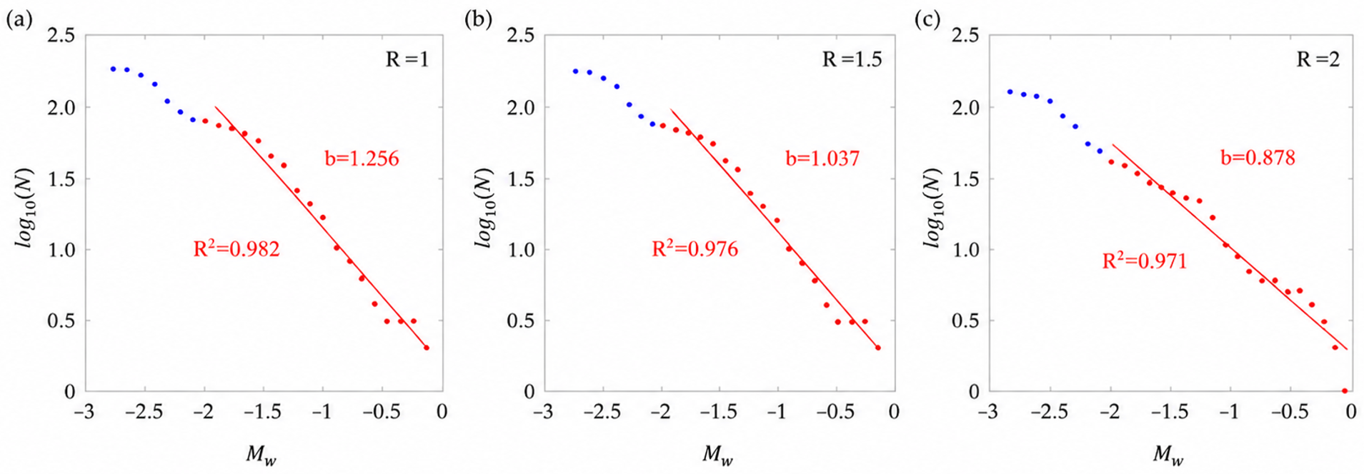
b-value fitting details are illustrated in Table 3. Figure 12 presents the cumulative magnitude-frequency distributions of induced seismic events in fractured rock under three different stress ratios. The dots denote the logarithm of the cumulative number of observed cumulative seismicity. Blue points correspond to lower-magnitude events at the tail of the distribution, whereas red points represent the magnitude range used for linear fitting. The solid red lines indicate the best-fit Gutenberg–Richter relationships, from which the b-values are estimated. A clear systematic trend is observed: the b-value decreases with increasing stress ratio. The resulting b-values are 1.256 for R = 1, 1.037 for R = 1.5, and 0.878 for R = 2, as labeled in each subplot.
Table 3.
b-value fitting details.
Figure 12.
Cumulative distribution of induced seismicity in the fractured rock subjected to different stress ratios.
For R = 1, the relatively high b-value indicates a dominance of small-magnitude events, suggesting more distributed micro-fracturing and limited stress concentration. As the stress ratio increases to R = 1.5 and R = 2, the slope of the fitted line becomes progressively flatter, reflecting a higher proportion of larger-magnitude events. This behavior implies enhanced stress concentration and a greater tendency for coherent fracture reactivation under higher differential stress conditions.
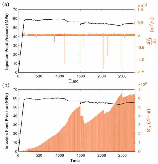
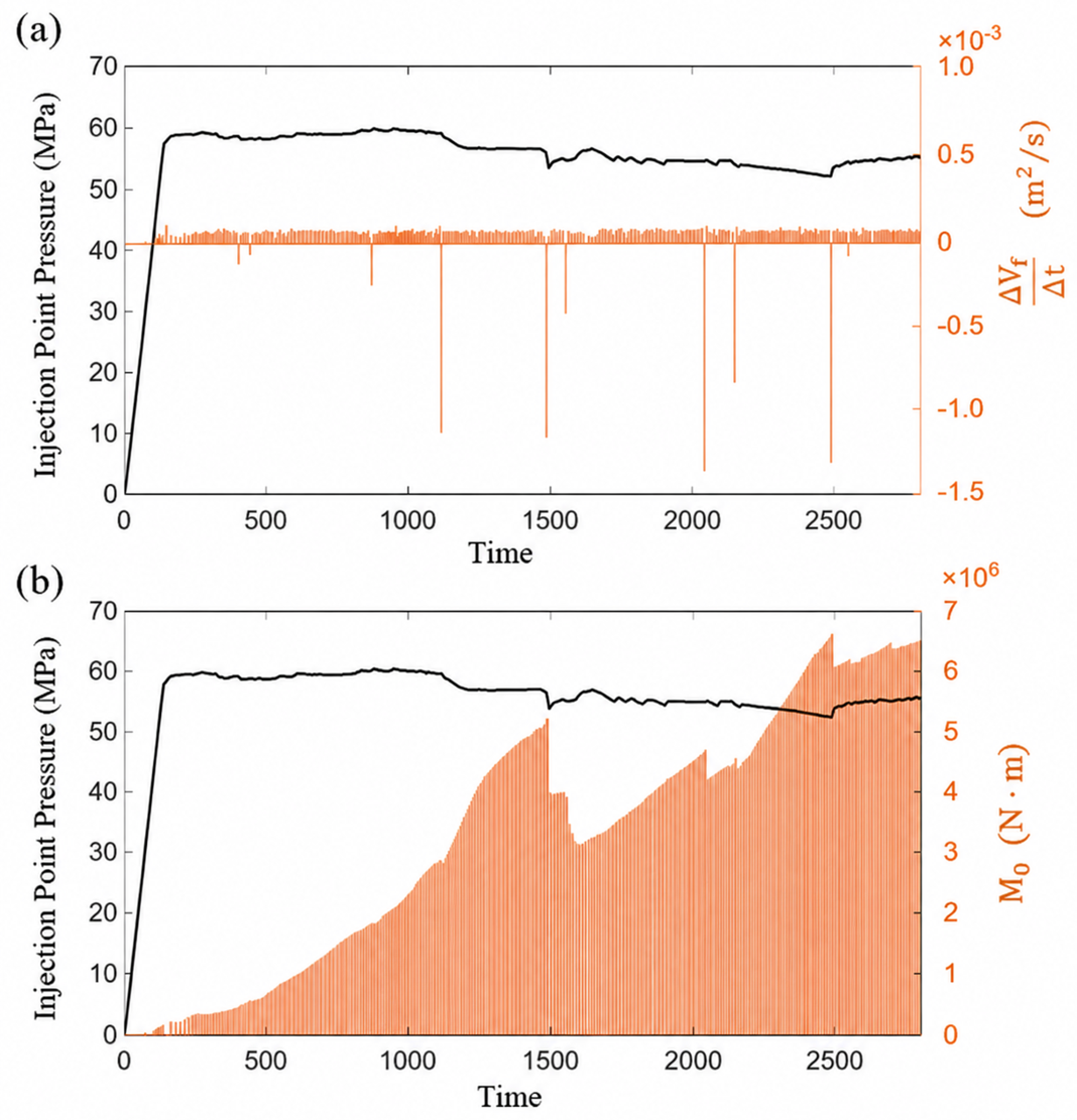
Unstable deformation and stress redistribution in geomechanical systems, providing a broader context for interpreting the observed intermittent fracture volume change rates and associated seismic moment fluctuations [60]. A higher stress ratio leads to more pronounced pressure fluctuations, providing clearer insights into the coupling between fracture propagation and induced seismicity. Accordingly, the case with a stress ratio of 2 was selected for detailed analysis. Figure 13 illustrates the temporal evolution of injection-induced fracture volume change rate and seismic moment in relation to injection-point pressure during fluid injection for R = 2. The black solid line represents the injection-point pressure plotted against time, while the orange bars represent different measures of fracture deformation or seismic response plotted on the right vertical axis. In Figure 13a, at the onset of injection, the pressure increases rapidly from zero to approximately 60 MPa. Thereafter, it remains relatively stable with only minor fluctuations, indicating the establishment of a quasi-steady injection regime. Despite the relatively stable pressure, the fracture volume change rate does not evolve smoothly. Instead, it exhibits multiple distinct positive and negative spikes, reflecting the episodic nature of fracture evolution. Positive spikes correspond to sudden fracture opening, rapid fracture growth, or coalescence of pre-existing fractures, whereas negative spikes indicate fracture closure, stress relaxation, or local damage redistribution following major deformation events. This behavior demonstrates that fracture propagation is governed by intermittent mechanical instabilities, rather than continuous pressure-driven growth.
Figure 13.
Temporal evolution of injection-induced fracture volume change rate and seismic moment in relation to injection-point pressure for R = 2. (a) Injection pressure and incremental fracture volume change rate; (b) injection pressure and cumulative seismic moment.
In Figure 13b, the orange bars indicate a cumulative increase in seismic moment over time, reflecting the ongoing release of elastic strain energy due to fracture slip and opening. Although seismic moment is generally considered a cumulative quantity, M0 exhibits a pronounced temporary decrease during episodes of sudden fracture opening or fracture reactivation. The timing of negative fracture volume change rates is highly consistent with the moments when the seismic moment exhibits sudden decreases. Newly activated fractures can redistribute stress away from previously active seismic sources. This stress redistribution may reduce slip rates or slip areas on earlier fractures, resulting in a net decrease in seismic moment contribution during new fracture propagation. The figure reveals that fracture propagation during fluid injection is dominated by episodic tensile opening and stress redistribution, whereas microseismicity primarily reflects localized shear slip, resulting in a clear decoupling between fracture volume growth and seismic moment release.
5. Conclusions
This investigation developed a fully coupled hydro-mechanical framework based on FDEM to systematically investigate fracture propagation and induced seismicity during hydraulic fracturing in naturally fractured rock. The main conclusions are as follows.
- (1)
- The in situ horizontal stress ratio exerts a primary control on hydraulic fracture propagation, fluid pressure evolution, and induced seismicity. Increasing stress anisotropy promotes a transition from diffuse, naturally fracture-controlled propagation to highly localized, stress-aligned fracture growth dominated by the principal stress field.
- (2)
- With increasing stress ratio, fluid pressure becomes progressively more concentrated within dominant fracture corridors, resulting in higher peak injection pressures and stronger pressure fluctuations. The evolution of mean stress and volumetric strain closely follows fluid pressure changes, confirming that effective stress reduction and rock dilation are primarily driven by fluid pressurization.
- (3)
- Higher stress ratios promote relatively larger seismic events and reduce the b-value. Higher stress ratios lead to more clustered and directional seismic event distributions and lower Gutenberg–Richter b-values, indicating a shift from distributed micro-fracturing toward more coherent fracture reactivation and relatively larger seismic events.
- (4)
- Even under quasi-steady injection pressure conditions, fracture propagation is inherently episodic and unstable. Fracture volume change rates display pronounced positive and negative spikes, reflecting intermittent fracture opening, closure, and stress redistribution rather than continuous pressure-driven growth.
- (5)
- Fracture volume growth and seismic moment release are not necessarily positively correlated. Episodes of negative fracture volume change closely coincide with abrupt, temporary reductions in seismic moment, indicating stress redistribution away from previously active seismic sources. This behavior demonstrates that tensile-dominated fracture opening can occur largely seismically, whereas induced seismicity is primarily controlled by localized shear slip.
- (6)
- For geothermal reservoirs and unconventional shale formations, well trajectories should be optimized to align with the maximum horizontal stress direction to enhance fracture controllability and minimize unintended fracture branching. In addition, lower injection rates and cyclic injection schemes are recommended to reduce stress concentration and mitigate the risk of fault reactivation.
Author Contributions
Y.L.: Writing—original draft, Data curation, Conceptualization. J.L.: Writing—original draft, Methodology, Data curation, Conceptualization. X.F.: Writing—review and editing, Methodology, Investigation. P.Y.: Methodology, Investigation, Formal analysis. Y.X.: Writing—review and editing, Writing—original draft, Investigation. H.L.: Writing—review and editing, Formal analysis, Data curation, Conceptualization. G.W. and W.L.: Writing—original draft, Resources, Formal analysis. All authors have read and agreed to the published version of the manuscript.
Funding
This work is financially supported by the National Natural Science Foundation of China (No. 52274231 and No. 52034006).
Data Availability Statement
Data will be made available on request.
Conflicts of Interest
The authors declare that they have no known competing financial interests or personal relationships that could have appeared to influence the work reported in this paper.
References
- Gao, D. Some research advances in well engineering technology for unconventional hydrocarbon. Nat. Gas Ind. B 2022, 9, 41–50. [Google Scholar] [CrossRef] [Scilit]
- Wang, K.; Yuan, B.; Ji, G.; Wu, X. A comprehensive review of geothermal energy extraction and utilization in oilfields. J. Pet. Sci. Eng. 2018, 168, 465–477. [Google Scholar] [CrossRef] [Scilit]
- Zhang, Y.; Zhao, G.F. A global review of deep geothermal energy exploration: From a view of rock mechanics and engineering. Geomech. Geophys. Geo-Energy Geo-Resour. 2020, 6, 4. [Google Scholar]
- Lei, Q.; Doonechaly, N.G.; Tsang, C.F. Modelling fluid injection-induced fracture activation, damage growth, seismicity occurrence and connectivity change in naturally fractured rocks. Int. J. Rock Mech. Min. Sci. 2021, 138, 104598. [Google Scholar] [CrossRef] [Scilit]
- Lu, W.; Yang, J.; Yan, P.; Chen, M.; Zhou, C.; Luo, Y.; Jin, L. Dynamic response of rock mass induced by the transient release of in-situ stress. Int. J. Rock Mech. Min. Sci. 2012, 53, 129–141. [Google Scholar] [CrossRef] [Scilit]
- Zhang, C.; Fan, D.; Elsworth, D.; He, M.; Zhao, X.; Zhu, C.; Zhang, H. Mechanisms of stress-and fluid-pressure-driven fault reactivation in Gonghe granite: Implications for injection-induced earthquakes. Int. J. Rock Mech. Min. Sci. 2024, 174, 105642. [Google Scholar]
- Kamali, A.; Ghassemi, A. On the reservoir stimulation mechanisms in fractured reservoirs. In ARMA US Rock Mechanics/Geomechanics Symposium; ARMA-2016; ARMA: Eaton, CO, USA, 2016. [Google Scholar]
- Dutler, N.; Valley, B.; Gischig, V.; Villiger, L.; Krietsch, H.; Doetsch, J.; Brixel, B.; Jalali, M.; Amann, F. Hydraulic fracture propagation in a heterogeneous stress field in a crystalline rock mass. Solid Earth 2019, 10, 1877–1904. [Google Scholar] [CrossRef] [Scilit]
- Hui, G.; Chen, Z.; Schultz, R.; Chen, S.; Song, Z.; Zhang, Z.; Song, Y.; Wang, H.; Wang, M.; Gu, F. Intricate unconventional fracture networks provide fluid diffusion pathways to reactivate pre-existing faults in unconventional reservoirs. Energy 2023, 282, 128803. [Google Scholar] [CrossRef] [Scilit]
- Li, X.F.; Li, X.; Li, H.B.; Zhang, Q.B.; Zhao, J. Dynamic tensile behaviours of heterogeneous rocks: The grain scale fracturing characteristics on strength and fragmentation. Int. J. Impact Eng. 2018, 118, 98–118. [Google Scholar] [CrossRef] [Scilit]
- Lei, Q. More is different: On the emergence of collective phenomena in fractured rocks. Rock Mech. Bull. 2023, 2, 100080. [Google Scholar] [CrossRef] [Scilit]
- Yang, K.; Liang, Y.; Li, Q. Macro-and-Micro Heterogeneous Influence on Fracture Morphology and Failure Modes during Hydraulic Fracturing of Coal: A Coupled Hydro-Mechanical-Damage Model. Rock Mech. Rock Eng. 2025, 1–26. [Google Scholar]
- Yuan, S.C.; Harrison, J.P. A review of the state of the art in modelling progressive mechanical breakdown and associated fluid flow in intact heterogeneous rocks. Int. J. Rock Mech. Min. Sci. 2006, 43, 1001–1022. [Google Scholar] [CrossRef] [Scilit]
- Taleghani, A.D.; Gonzalez, M.; Shojaei, A. Overview of numerical models for interactions between hydraulic fractures and natural fractures: Challenges and limitations. Comput. Geotech. 2016, 71, 361–368. [Google Scholar] [CrossRef] [Scilit]
- Jin, Y.; He, C.; Yao, C.; Sun, Z.; Zhang, X.; Yang, J.; Jiang, Q.; Zhou, C. Effects of in-situ stress on heat transfer in fracture networks. Geomech. Energy Environ. 2024, 37, 100516. [Google Scholar]
- Wang, S.; Zhou, J.; Zhang, L.; Han, Z.; Kong, Y. Modeling interactions between hydraulic and closed natural fractures in brittle crystalline rocks: A Fluid–Solid coupling Grain-Based approach for characterizing microcracking behaviors. Rock Mech. Rock Eng. 2024, 57, 889–920. [Google Scholar]
- Zhang, Y.; Zhang, J.; Yuan, B.; Yin, S. In-situ stresses controlling hydraulic fracture propagation and fracture breakdown pressure. J. Pet. Sci. Eng. 2018, 164, 164–173. [Google Scholar] [CrossRef] [Scilit]
- Duan, K.; Kwok, C.Y.; Zhang, Q.; Shang, J. On the initiation, propagation and reorientation of simultaneously-induced multiple hydraulic fractures. Comput. Geotech. 2020, 117, 103226. [Google Scholar] [CrossRef] [Scilit]
- Ding, Z.; Feng, X.; Wang, E.; Cao, Z. Fault slip mechanics and seismic source characteristics considering fracture zone anisotropy. Acta Geotech. 2025, 20, 3411–3437. [Google Scholar] [CrossRef] [Scilit]
- Garagash, I.A.; Osiptsov, A.A. Fracture propagation in an initially stressed anisotropic reservoir under shear: Reorientation and fluid lag. Eng. Fract. Mech. 2021, 242, 107457. [Google Scholar] [CrossRef] [Scilit]
- Liu, G.; Ma, F.; Zhang, M.; Guo, J.; Jia, J. Y-Mat: An improved hybrid finite-discrete element code for addressing geotechnical and geological engineering problems. Eng. Comput. 2022, 39, 1962–1983. [Google Scholar]
- Adelinet, M.; Dorbath, C.; Calò, M.; Dorbath, L.; Le Ravalec, M. Crack features and shear-wave splitting associated with fracture extension during hydraulic stimulation of the geothermal reservoir in Soultz-sous-Forets. Oil Gas Sci. Technol. 2016, 71, 39. [Google Scholar]
- Aimene, Y.E.; Ouenes, A. Geomechanical modeling of hydraulic fractures interacting with natural fractures—Validation with microseismic and tracer data from the Marcellus and Eagle Ford. Interpretation 2015, 3, SU71–SU88. [Google Scholar]
- Haque, E.A.; Shofiullah, S. Hydrogen embrittlement sensitivity of additively manufactured 347H stainless steel: Effects of porosity and residual stress. Int. J. Sci. Interdiscip. Res. 2023, 4, 100–144. [Google Scholar] [CrossRef] [Scilit]
- Pischiutta, M.; Salvini, F.; Fletcher, J.; Rovelli, A.; Ben-Zion, Y. Horizontal polarization of ground motion in the Hayward fault zone at Fremont, California: Dominant fault-high-angle polarization and fault-induced cracks. Geophys. J. Int. 2012, 188, 1255–1272. [Google Scholar] [CrossRef] [Scilit]
- Atkinson, G.M.; Eaton, D.W.; Igonin, N. Developments in understanding seismicity triggered by hydraulic fracturing. Nat. Rev. Earth Environ. 2020, 1, 264–277. [Google Scholar] [CrossRef] [Scilit]
- Butt, A.; Hedayat, A.; Moradian, O. Microseismic monitoring of laboratory hydraulic fracturing experiments in granitic rocks for different fracture propagation regimes. Rock Mech. Rock Eng. 2024, 57, 2035–2059. [Google Scholar]
- Van Der Baan, M.; Eaton, D.; Dusseault, M. Microseismic monitoring developments in hydraulic fracture stimulation. In ISRM International Conference for Effective and Sustainable Hydraulic Fracturing; ISRM: Lisbon, Portugal, 2013. [Google Scholar]
- Zhang, F.; Chen, Y.; Wang, R.; Yu, H.; Chen, H.; Liu, F.; Shi, X. Integrated analysis of seismic sources and structures: Understanding earthquake clustering during hydraulic fracturing. J. Geophys. Res. Solid Earth 2025, 130, e2024JB030008. [Google Scholar] [CrossRef] [Scilit]
- Belytschko, T.; Black, T. Elastic crack growth in finite elements with minimal remeshing. Int. J. Numer. Methods Eng. 1999, 45, 601–620. [Google Scholar] [CrossRef] [Scilit]
- Hamdi, P.; Stead, D.; Elmo, D. Damage characterization during laboratory strength testing: A 3D-finite-discrete element approach. Comput. Geotech. 2014, 60, 33–46. [Google Scholar] [CrossRef] [Scilit]
- Liu, C.; Zhang, F.; Detournay, E. Finite domain solution of a hydraulic fracture in a permeable rock. Rock Mech. Bull. 2025, 4, 100156. [Google Scholar] [CrossRef] [Scilit]
- Ziebarth, R.A.; Corkum, A.G.; Walton, G. Development and Evaluation of a Continuum-based Jointed Rock Mass Model. Rock Mech. Rock Eng. 2025, 58, 12817–12835. [Google Scholar] [CrossRef] [Scilit]
- Garipov, T.T.; Karimi-Fard, M.; Tchelepi, H.A. Discrete fracture model for coupled flow and geomechanics. Comput. Geosci. 2016, 20, 149–160. [Google Scholar] [CrossRef] [Scilit]
- Profit, M.; Dutko, M.; Yu, J.; Cole, S.; Angus, D.; Baird, A. Complementary hydro-mechanical coupled finite/discrete element and microseismic modelling to predict hydraulic fracture propagation in tight shale reservoirs. Comput. Part. Mech. 2016, 3, 229–248. [Google Scholar] [CrossRef] [Scilit]
- Lisjak, A.; Grasselli, G.; Vietor, T. Continuum–discontinuum analysis of failure mechanisms around unsupported circular excavations in anisotropic clay shales. Int. J. Rock Mech. Min. Sci. 2014, 65, 96–115. [Google Scholar] [CrossRef] [Scilit]
- Lisjak, A.; Tatone, B.S.A.; Kaifosh, P.; He, L.; Mahabadi, O.K.; Grasselli, G. Development of a fully-coupled, hydro-mechanical model for finite-discrete element simulations of fluid-driven fracturing. In ARMA US Rock Mechanics/Geomechanics Symposium; ARMA: Eaton, CO, USA, 2016. [Google Scholar]
- Lisjak, A.; Mahabadi, O.K.; Andersen, J.; Hinkey, J.; Detournay, E.; Araujo, E.; Rimmelin, R. Development of a novel dynamic formation stimulation technique: FDEM-based numerical modelling results. In ARMA US Rock Mechanics/Geomechanics Symposium; ARMA: Eaton, CO, USA, 2023. [Google Scholar]
- Munjiza, A.A. The Combined Finite-Discrete Element Method; John Wiley & Sons: Hoboken, NJ, USA, 2004. [Google Scholar]
- Zhao, Q.; Lisjak, A.; Mahabadi, O.; Liu, Q.; Grasselli, G. Numerical simulation of hydraulic fracturing and associated microseismicity using finite-discrete element method. J. Rock Mech. Geotech. Eng. 2014, 6, 574–581. [Google Scholar] [CrossRef] [Scilit]
- AbuAisha, M.; Eaton, D.; Priest, J.; Wong, R. Hydro-mechanically coupled FDEM framework to investigate near–wellbore hydraulic fracturing in homogeneous and fractured rock formations. J. Pet. Sci. Eng. 2017, 154, 100–113. [Google Scholar]
- Deng, P.; Liu, Q.; Huang, X.; Pan, Y.; Wu, J. FDEM numerical modeling of failure mechanisms of anisotropic rock masses around deep tunnels. Comput. Geotech. 2022, 142, 104535. [Google Scholar] [CrossRef] [Scilit]
- Muhammad, K.; Liu, H.; Daisuke, F.; Peng, J.; Gyeongjo, M.; Chan, A. State-of-the-Art Review and Prospect of Modelling the Dynamic Fracture of Rocks Under Impact Loads and Application in Blasting. Geosciences 2025, 15, 314. [Google Scholar] [CrossRef] [Scilit]
- Farsi, A.; Xiang, J.; Latham, J.P.; Carlsson, M.; Stitt, H.; Marigo, M. Packing simulations of complex-shaped rigid particles using FDEM: An application to catalyst pellets. Powder Technol. 2021, 380, 443–461. [Google Scholar] [CrossRef] [Scilit]
- Knight, E.E.; Rougier, E.; Lei, Z.; Euser, B.; Chau, V.; Boyce, S.H.; Ke, G.; Okubo, K.; Froment, M. HOSS: An implementation of the combined finite-discrete element method. Comput. Part. Mech. 2020, 7, 765–787. [Google Scholar] [CrossRef] [Scilit]
- Mahabadi, O.K.; Grasselli, G.; Munjiza, A. Y-GUI: A graphical user interface and pre-processor for the combined finite-discrete element code, Y2D, incorporating material heterogeneity. Comput. Geosci. 2010, 36, 241–252. [Google Scholar] [CrossRef] [Scilit]
- Mahabadi, O.K.; Lisjak, A.; He, L.; Tatone, B.S.A.; Kaifosh, P.; Grasselli, G. Development of a new fully-parallel finite-discrete element code: Irazu. In ARMA US Rock Mechanics/Geomechanics Symposium; ARMA: Eaton, CO, USA, 2016. [Google Scholar]
- Irazu Geomechanical Simulation Software; Geomechanica Inc.: Toronto, ON, Canada, 2024.
- Wu, D.; Li, H.; Fukuda, D.; Liu, H. Development of a finite-discrete element method with finite-strain elasto-plasticity and cohesive zone models for simulating the dynamic fracture of rocks. Comput. Geotech. 2023, 156, 105271. [Google Scholar] [CrossRef] [Scilit]
- Sun, L.; Tang, X.; Aboayanah, K.R.; Xu, X.; Liu, Q.; Grasselli, G. Coupled hydro-mechanical two-phase flow model in fractured porous medium with the combined finite-discrete element method. Eng. Comput. 2024, 40, 2513–2535. [Google Scholar] [CrossRef] [Scilit]
- Shandilaya, S.; Roshankhah, S. Hydro-Mechanical coupling of CO2 injection into homogeneous and naturally fractured rock mass with permeable matrix. In ARMA US Rock Mechanics/Geomechanics Symposium; ARMA: Eaton, CO, USA, 2025; p. D031S029R002. [Google Scholar]
- Sharafisafa, M.; Aliabadian, Z.; Sato, A.; Shen, L. Coupled thermo-hydro-mechanical simulation of hydraulic fracturing in deep reservoirs using finite-discrete element method. Rock Mech. Rock Eng. 2023, 56, 5039–5075. [Google Scholar]
- Lukin, O.; Kondrat, O. Utilizing well-reservoir pseudo-connections for multi-stage hydraulic fracturing modeling in tight gas saturated formations. Min. Miner. Depos. 2024, 18, 113–121. [Google Scholar] [CrossRef] [Scilit]
- Farkas, M.P.; Hofmann, H.; Zimmermann, G.; Zang, A.; Zhuang, L.; Kim, K.Y. Numerical investigation of laboratory hydraulic fracturing tests in Pocheon granite. Acta Geotech. 2023, 18, 2011–2038. [Google Scholar]
- Kanamori, H.; Brodsky, E.E. The physics of earthquakes. Phys. Today 2001, 54, 34–40. [Google Scholar] [CrossRef] [Scilit]
- Bormann, P.; Di Giacomo, D. The moment magnitude Mw and the energy magnitude Me: Common roots and differences. J. Seismol. 2011, 15, 411–427. [Google Scholar]
- Scholz, C.H. The Mechanics of Earthquakes and Faulting; Cambridge University Press: Cambridge, UK, 2019. [Google Scholar]
- Mussin, R.; Małkowski, P.; Murtazina, F.; Kainazarova, A.; Akhmatnurov, D.; Zamaliyev, N.; Doni, D. Integrated geophysical assessment of coal mass structural weakening zones for optimization of drilling-blasting operations and coal size control. Min. Miner. Depos. 2025, 19, 99–118. [Google Scholar] [CrossRef] [Scilit]
- Tan, Z.; Zhao, J.; Li, Z.; Zhang, B. A study on surrounding rock characteristics inducing severe large deformation in tunnels and methods for determining its strength. Sci. Rep. 2025, 15, 7011. [Google Scholar] [CrossRef] [Scilit] [PubMed]
- Petlovanyi, M.; Sai, K. Numerical modelling of critical conditions for the onset of a limit state in the rock mass surrounding unfilled underground voids in iron ore deposits. Eng. J. Satbayev Univ. 2026, 148, 38–47. [Google Scholar] [CrossRef] [Scilit]

Disclaimer/Publisher’s Note: The statements, opinions and data contained in all publications are solely those of the individual author(s) and contributor(s) and not of MDPI and/or the editor(s). MDPI and/or the editor(s) disclaim responsibility for any injury to people or property resulting from any ideas, methods, instructions or products referred to in the content. |
© 2026 by the authors. Licensee MDPI, Basel, Switzerland. This article is an open access article distributed under the terms and conditions of the Creative Commons Attribution (CC BY) license.