


Highlights
What are the main findings?
- •
- A forecast-augmented RF–GB–SVM ensemble controller achieved 0.83 °C temperature RMSE during 28 days of continuous greenhouse deployment.
- •
- Forecast integration enabled proactive irrigation suppression before rainfall events, reducing pump operating time by 18% without degrading soil moisture compliance.
- •
- The proposed ensemble controller achieved lower temperature-tracking error than the threshold-based and PID reference baselines under the adopted disturbance-consistent evaluation protocol.
- •
- Feature ablation and explainability analysis confirmed the dominant contribution of forecast-derived variables to anticipatory control performance.
What are the implications of the main findings?
- •
- Low-cost edge AI hardware can support practical multi-variable greenhouse control without computationally intensive optimisation.
- •
- Forecast-driven feedforward control improves water-use efficiency and operational sustainability in greenhouse environments.
- •
- The proposed framework provides a deployable foundation for future adaptive and large-scale intelligent greenhouse systems.
Abstract
Greenhouse microclimate regulation is challenging due to nonlinear coupling among temperature, humidity, soil moisture, and light intensity, which limits the effectiveness of conventional threshold-based and PID control strategies under time-varying environmental disturbances. This paper presents a forecast-augmented ensemble control framework that combines Random Forest, Gradient Boosting, and Support Vector Machine classifiers with one-hour-ahead weather forecasts for closed-loop greenhouse microclimate regulation. The proposed system was deployed and validated in a working greenhouse cultivating cucumber (cv. ‘Madora F1’) over 28 consecutive days. Sensor measurements and forecast inputs were processed through a unified preprocessing pipeline, while control actions were generated through majority voting and executed on Raspberry Pi 4B edge hardware with a worst-case inference latency below 18 ms. The proposed framework achieved a temperature RMSE of 0.83 °C during field deployment. For reference, RMSE values of 3.21 °C and 1.94 °C were obtained for the threshold-based and PID baseline controllers, respectively, under the adopted disturbance-consistent evaluation protocol. Compliance rates reached 96.4% for temperature, 94.1% for relative humidity, and 97.2% for soil moisture across 40,320 resampled observation intervals (60 s analysis grid) derived from the original 10 s acquisition stream. Integration of short-term weather forecasts enabled anticipatory irrigation management, reducing irrigation pump operation by 18% without compromising soil-moisture compliance and yielding an estimated annual energy saving of 158 kWh per greenhouse zone. Unlike prediction-oriented greenhouse artificial-intelligence studies, the proposed approach implements a deployable forecast-augmented closed-loop control architecture validated under continuous real-world greenhouse operation.
1. Introduction
Greenhouse cultivation is increasingly important as climatic variability intensifies [1]. Keeping temperature, humidity, light, and soil moisture within crop-specific ranges is essential for consistent plant growth [2,3], as sustained deviations lead to yield loss and reduced quality.
Conventional greenhouse control methods have well-known limitations. Manual operation introduces delays and inconsistency, while fixed-threshold controllers cannot capture nonlinear interactions or adapt to changing environmental conditions [4,5]. PID-based approaches improve single-variable regulation but require independent tuning and degrade under time-varying disturbances such as solar radiation and crop growth [6]. Moreover, these approaches remain reactive and cannot incorporate predictive weather information.
Advances in IoT sensing and machine learning have made data-driven greenhouse control increasingly practical [4,7]. Prior studies report improved prediction accuracy and energy efficiency using neural networks and ensemble models [3,5,7,8,9,10]. However, several limitations remain: most systems regulate only a subset of variables, validation is often short-term or simulation-based, forecast data are rarely used as feedforward inputs [11,12,13,14], and feature design is typically empirical rather than model-based. A structured examination of representative prior work highlights the following specific gaps. Neural network and deep learning approaches [3,8,15,16] achieve competitive prediction accuracy but are trained without an explicit control objective and are rarely validated in closed-loop field settings beyond 14 days. MPC-based formulations [17] provide a structured framework and can in principle exploit forecast data, but require accurate full-order plant models and online optimisation solvers that are incompatible with resource-constrained edge hardware. Forecast-driven irrigation systems [11,12,13,14] demonstrate the value of weather-predictive feedforward for a single actuator, but do not extend to multi-variable microclimate regulation. AI-powered multi-variable control systems [7] address the joint regulation problem but omit forecast integration and provide validation periods shorter than 21 days. Existing studies rarely combine all of the following characteristics simultaneously: (i) multi-variable closed-loop control of T, RH, SM, and L; (ii) forecast-based feedforward; (iii) model-guided feature design; and (iv) continuous field validation exceeding 21 days.
In addition, most existing AI-based greenhouse studies focus primarily on prediction accuracy rather than real-time control implementation under hardware and actuator constraints. In contrast, the proposed system is designed as a deployable edge-control architecture operating directly within a closed-loop greenhouse environment.
This study addresses the above limitations through four main contributions.
First, a discrete-time dynamic model of greenhouse thermal and soil moisture dynamics is integrated with the machine learning framework, guiding feature design and linking physical variables to the multi-variable control objective.
Second, short-horizon weather forecast data are incorporated as a feedforward input, enabling anticipatory control actions such as proactive irrigation suppression prior to precipitation events, which cannot be achieved by purely feedback-based approaches [12,13,14].
Third, the proposed AI ensemble controller is validated through 28 days of continuous real-world greenhouse operation, representing among the longer continuous field validations reported for ML-based greenhouse control systems.
Fourth, the ensemble decision mechanism can be interpreted as an approximate one-step decision policy over the binary actuator space, providing a practical interpretation of the ensemble output within the control system.
Together, these contributions form a greenhouse control system that links physical modelling, data-driven learning, and weather forecast inputs. The goal is practical: stable multi-variable regulation on low-cost hardware, validated in a real growing environment.
2. Greenhouse Dynamics Modelling and Control Problem Formulation
2.1. Physical Coupling and State Variables
A greenhouse constitutes a semi-enclosed thermo-hydraulic system whose internal microclimate is governed by the coupled interaction of solar irradiance, ambient temperature and humidity, crop transpiration, and anthropogenic actuator inputs. The four primary controllable state variables are air temperature T (°C), relative humidity RH (%), volumetric soil moisture SM (% VWC), and light intensity L (lux). These variables are physically coupled: heater activation raises T and simultaneously reduces RH through increased saturation vapour pressure; forced ventilation reduces both T and RH; irrigation replenishes SM and contributes marginal RH increase through surface evaporation; shade tents attenuate L and moderate T through reduced solar thermal gain. This physical coupling makes single-loop independent control strategies inherently suboptimal and motivates the multi-variable formulation adopted here.
2.2. Discrete-Time Dynamic Model
A discrete-time model of greenhouse thermal and soil moisture dynamics is formulated to guide feature selection and link the physical process to the control objective [17], following classical transfer-function-based process modelling approaches [18]. The sampling period is , consistent with the PLC acquisition cycle.
The model rests on three simplifying assumptions: well-mixed air volume, lumped latent heat effects, and spatially averaged root-zone moisture. Unmodelled effects are captured by disturbance terms and .
Under these assumptions, the thermal dynamics are described by:
where is the internal air temperature, is the external temperature, is the heater control input, and is the solar irradiance proxy derived from light intensity and cloud cover. The disturbance term aggregates unmodelled effects such as ventilation losses and crop transpiration.
The soil moisture subsystem is described by:
where is the spatially averaged volumetric soil moisture, is the irrigation command, and is the evapotranspiration rate estimated from using a simplified Penman–Monteith proxy [19]. The disturbance term includes unmodelled effects such as precipitation.
The precipitation probability obtained from the forecast API acts as a predictive estimate of the disturbance term , and provides a physical basis for its inclusion in the feature vector. It should be noted that forecast precipitation is not interpreted as direct water input to the greenhouse root zone, since the greenhouse structure prevents direct rainfall infiltration into the cultivated soil. Instead, precipitation forecasts serve as an indirect predictor of irrigation demand by indicating environmental conditions associated with reduced solar radiation, lower evapotranspiration rates, increased ambient humidity, and consequently lower expected water consumption.
Model parameters were estimated from step-response experiments using constrained least-squares minimisation, yielding a1 = 0.042, a2 = 1.83 °C per activation step, a3 = 0.0071, b1 = 0.31% VWC per activation step, and b2 = 0.0038 VWC per unit evapotranspiration. The resulting models achieved R2 = 0.978 (thermal) and R2 = 0.961 (soil moisture). Sensitivity analysis under ±20% parameter perturbations resulted in RMSE variations within 8–23%, which is acceptable for practical control design.
It should be noted that the discrete-time dynamic models in Equations (1) and (2) cover only the thermal (T) and soil moisture (SM) subsystems, for which physically parameterised step-response data were available. Relative humidity (RH) and light intensity (L) are not explicitly modelled at this stage because their dominant dynamics—vapour-pressure equilibration and solar irradiance, respectively—are strongly driven by external boundary conditions that cannot be independently actuated within the single-zone facility. These variables are nevertheless included in the multi-variable control objective J (Equation (3)) and in the ensemble feature vector, allowing the classifiers to learn their regulation empirically from the labelled dataset. The dynamic models thus serve the specific purpose of motivating feature selection and providing physical grounding for the T and SM terms in J; they are not intended to constitute a full MIMO plant model for all four subsystems.
2.3. Multi-Variable Control Objective
The regulation objective is to minimise a weighted quadratic tracking error over the operational horizon:
where λi ≥ 0 are weighting coefficients reflecting crop sensitivity. The weights λ1 = 1.0, λ2 = 0.6, λ3 = 0.8, and λ4 = 0.4 are assigned based on agronomic sensitivity rankings [5], prioritising temperature and soil moisture.
Directly minimising this objective over binary actuator inputs is not practical for real-time edge hardware. The ensemble classifier instead produces an approximate one-step decision policy over the discrete action space, learned from observed state–action pairs during the pre-deployment period.
2.4. Baseline Control Methods
To contextualise the performance of the proposed AI ensemble, two baseline strategies are defined: a threshold-based controller (TB-Baseline) and a PID controller (PID-Baseline). Neither baseline was physically deployed; instead, the threshold controller was evaluated through retrospective replay of the field dataset, while the PID controller was assessed via analytical simulation based on the identified models in Equations (1) and (2). This avoids the need for multi-zone physical partitioning while enabling fair comparison under identical disturbance inputs.
Simultaneous physical deployment of multiple controllers was not feasible because all actuators operated within a single shared greenhouse volume, making environmental isolation impossible without structural partitioning.
The threshold-based controller applies fixed hysteresis rules. The heater activates when and deactivates above . The irrigation pump activates when % VWC and deactivates above % VWC. The fan activates when or , and the shade tent when lux. No forecast input is used. Performance is obtained by replaying these rules on the recorded field dataset.
The PID baseline applies independent discrete-time controllers for temperature and soil moisture [15,20].
Parameters ( for temperature; for soil moisture) were derived from the identified model parameters using Ziegler–Nichols-based tuning [15,20]. The controller is evaluated through numerical simulation under measured disturbance sequences , and .
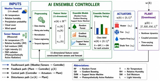
To ensure a fair comparison, the PID implementation includes standard industrial refinements: anti-windup clamping using back-calculation with , and a first-order derivative filter with . These modifications eliminate instability observed in the unmodified controller and provide a realistic reference for comparison. The relationship among control strategies is illustrated in Figure 1.
Figure 1.
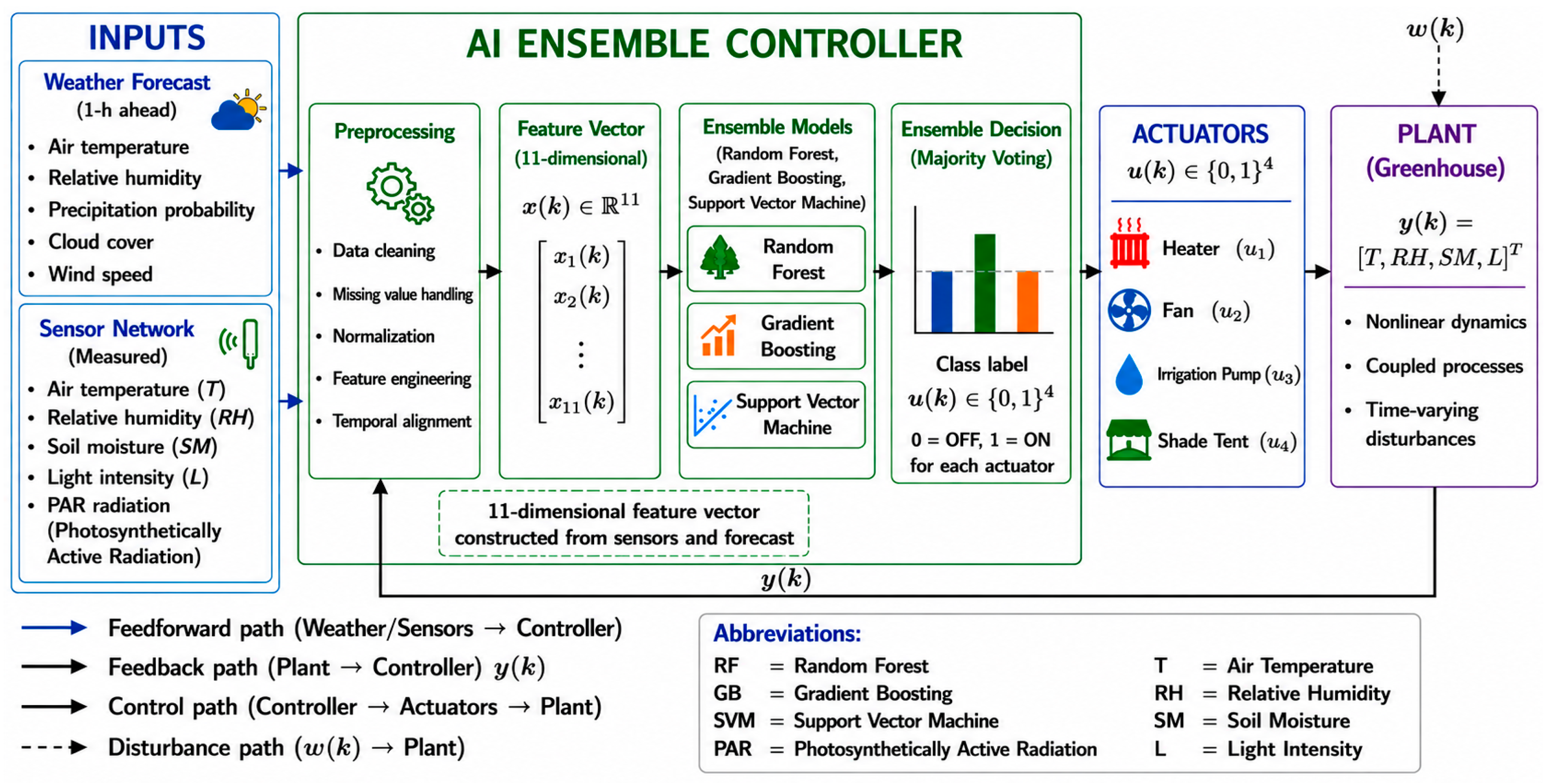
Forecast-augmented greenhouse control architecture used for closed-loop microclimate regulation. Weather forecasts and sensor measurements are fused into an 11-dimensional feature vector and processed by an ensemble of RF, GB, and SVM classifiers. Ensemble decisions are generated via majority voting and applied to four greenhouse actuators (heater, fan, irrigation pump, and shade tent). The system combines feedforward forecast information with feedback from greenhouse outputs (T, RH, SM, and L) to support adaptive microclimate regulation under external disturbances.
All controllers were evaluated under identical archived disturbance trajectories extracted from the same greenhouse deployment period, ensuring disturbance-consistent comparison despite differing implementation modalities (field deployment for the AI ensemble, retrospective replay for the threshold controller, and closed-loop simulation for the PID controller).
2.5. MPC Baseline Considerations
A natural comparator is Model Predictive Control (MPC), which can in principle exploit the same discrete-time models and forecast inputs. MPC was not deployed as a baseline because online QP solving over binary actuator states exceeds the compute budget of the target edge hardware, and the identified models cover only two of the four subsystems required for a full MIMO formulation. The objective here is to demonstrate a deployment-ready alternative; formal MPC comparison is reserved for future work.
Figure 1 illustrates the operational structure of the proposed greenhouse microclimate regulation system. Weather forecast information and real-time sensor measurements are merged into an 11-dimensional feature vector , which is processed by the RF–GB–SVM ensemble controller to generate binary actuator commands u(k).
The proposed framework follows a feature-level MIMO architecture where multiple environmental variables and actuator states are represented within a shared feature space. Unlike conventional single-loop PID approaches, the system captures cross-variable interactions through the common feature representation, while actuator decisions are generated independently at the ensemble output stage (Section 4.2).
The generated control commands drive the greenhouse actuators, while the plant output is continuously fed back into the controller. External disturbances , including weather fluctuations and solar radiation changes, influence the greenhouse dynamics during operation.
The feedforward branch based on OpenWeatherMap forecasts is intentionally separated from the feedback loop because forecast variables are independent of instantaneous sensor measurements. Therefore, forecast-derived parameters are treated as a distinct feature group within the classifier input vector described in Section 4.1.
3. System Architecture and Data Acquisition Methodology
The field deployment was carried out at an experimental greenhouse located on the grounds of Karshi State Technical University, Karshi, Kashkadarya region, Uzbekistan (approximately 38.86° N, 65.79° E, ~370 m above sea level). The facility is a single-zone structure with a floor area of 54 m2 (6 m × 9 m), framed in galvanised steel and enclosed with glass glazing. It was used to cultivate cucumber (Cucumis sativus L., cv. ‘Madora F1’), with 108 plants grown on parallel rows, and the monitored period spanned the vegetative and early-fruiting growth stages of the crop. Data collection comprised a 10-day pre-deployment training period followed by 28 consecutive days of autonomous operation, conducted during the spring season from 12 March to 18 April 2026. The local climate is continental and semi-arid, with a high diurnal temperature amplitude and strong daytime solar irradiance that together define the principal thermal disturbance regime addressed by the controller. The agronomic target bands used throughout this study are consistent with the operating ranges adopted for cucumber under protected cultivation.
3.1. Sensor Infrastructure and Measurement Subsystem
The measurement subsystem comprises five sensor types used for environmental monitoring and actuator control. Air temperature and relative humidity sensors are mounted at canopy height near the geometric centre of the greenhouse to minimise boundary-layer bias. Soil moisture is measured using two spatially separated root-zone probes, and their spatial average is used as the soil moisture feature in the classifier input vector [21,22]. The acquisition infrastructure also includes PAR radiation sensing and OpenWeatherMap (OWM) forecast integration for proactive control functionality. Here, PAR denotes Photosynthetically Active Radiation, while VWC refers to volumetric water content. The sensor and data acquisition infrastructure used in the experimental greenhouse is summarized in Table 1.
Table 1.
Sensor and data acquisition infrastructure.
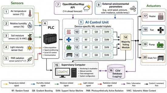
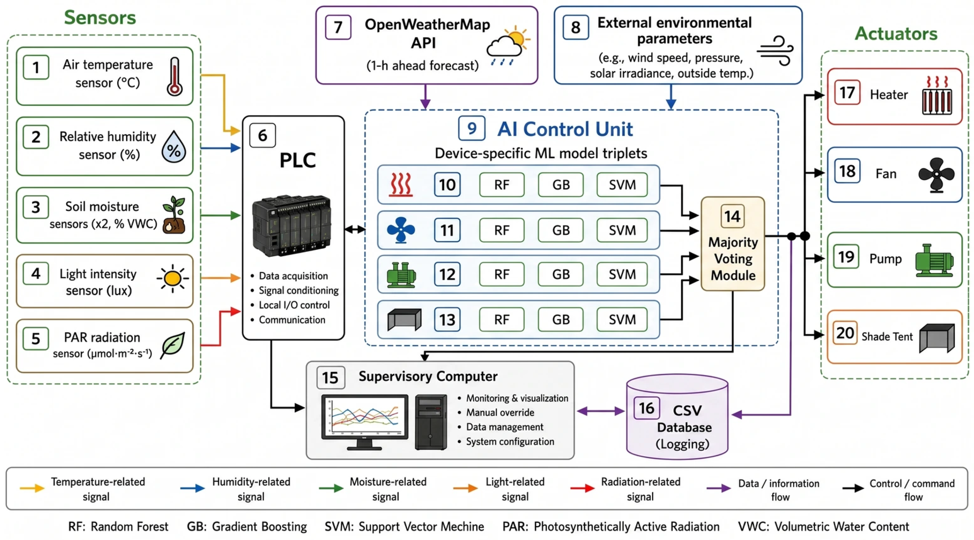
All sensor signals are acquired by a Programmable Logic Controller (PLC) at a fixed 10 s sampling interval. External weather forecasts retrieved from the OpenWeatherMap REST API every 60 s are incorporated as exogenous input features and merged with local sensor observations in a CSV-based database. The system integrates environmental sensing, forecast acquisition, ensemble inference, and actuator control within a unified edge-computing architecture.
The layered architecture includes microclimate sensors for temperature, humidity, soil moisture, light intensity, and PAR radiation, together with a forecast-processing module connected to the OpenWeatherMap service. The ensemble control unit applies majority voting across RF, GB, and SVM classifiers to generate actuator commands for the heater, ventilation fan, irrigation pump, and shade tent. The overall data and control flow used in the deployment is illustrated in Figure 2.
Figure 2.
Layered architecture of the proposed forecast-augmented greenhouse control system. Multi-source environmental data acquired from temperature, humidity, soil moisture, light-intensity, and PAR sensors are integrated with weather-forecast information through a PLC-based acquisition layer. Device-specific RF–GB–SVM ensemble models generate actuator commands for the heater, fan, irrigation pump, and shade tent, while a majority-voting mechanism produces the final control decision. A supervisory computer and logging database provide monitoring, configuration, and data-management functions for closed-loop greenhouse operation.
3.2. Data Preprocessing Pipeline
Raw sensor streams contain three primary sources of artefacts: spatial heterogeneity between the two soil moisture probes, non-stationarity of diurnal patterns under integer timestamp encoding, and impulse outliers caused by electrical interference or transient sensor disconnections. The accuracy of the one-hour-ahead OpenWeatherMap forecast inputs was characterised against co-located measurements over the deployment period. Mean absolute forecast errors were 1.23 °C for temperature ( vs. measured ), 4.2% for precipitation probability in binary threshold terms, and 11.4% for cloud cover fraction. These errors are substantially smaller than the inter-class decision margins learned by the classifiers (verified via margin analysis on SVM decision boundaries), indicating that forecast uncertainty does not significantly degrade the feedforward benefit. Forecast outages occurred in 0.8% of sampling intervals and were handled by substituting training-set mean values, consistent with the counterfactual analysis in Section 5.6.
To address these effects, a five-step preprocessing pipeline is applied consistently during both training and inference to ensure feature-space consistency and prevent data leakage.
Step 1 (spatial averaging): .
Step 2 (sinusoidal temporal encoding): the UTC timestamp t is encoded using sinusoidal functions, as defined below.
Step 3 (min–max normalisation): all continuous features are scaled to using parameters estimated from the training set only.
Step 4 (IQR-based outlier suppression): values beyond are replaced by a rolling median.
Step 5 (gap interpolation): missing values (up to three samples) are reconstructed via linear interpolation.
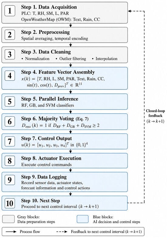
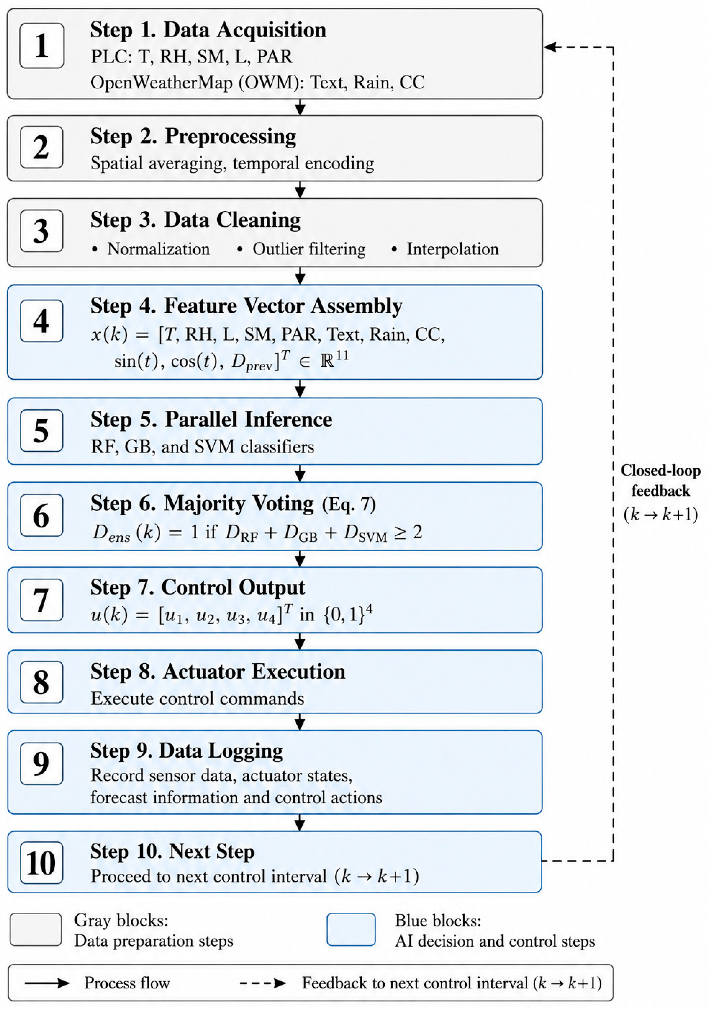
The processing sequence is illustrated in Figure 3. Each block corresponds to a deterministic operation; the absence of ambiguous or heuristic steps is a design choice ensuring that the algorithm is reproducible and PLC-deployable without modification. The sinusoidal temporal encoding in Step 2 is essential for continuity of the time-of-day feature across midnight boundaries—a property that integer hour encoding does not satisfy. The IQR-based outlier suppression in Step 4 is applied with parameters estimated exclusively from the training split, preventing any leakage of test-set statistics into the preprocessing stage.
Figure 3.
Sequential workflow of the forecast-augmented AI ensemble control framework. Raw sensor measurements and weather-forecast variables are subjected to preprocessing, data-cleaning, and feature-engineering operations before being assembled into an 11-dimensional feature vector. Device-state decisions are generated through parallel Random Forest (RF), Gradient Boosting (GB), and Support Vector Machine (SVM) classification and combined using a majority-voting strategy. The resulting binary control vector is transmitted to the greenhouse actuators, after which environmental states and control actions are recorded and used in the subsequent control interval, thereby establishing a closed-loop decision-making process. Abbreviations: T, air temperature; RH, relative humidity; SM, soil moisture; L, light intensity; PAR, photosynthetically active radiation; Text, external temperature; Rain, precipitation; CC, cloud cover.
Steps 1–2 perform sensor measurement acquisition and OpenWeatherMap forecast retrieval. Steps 3–4 include spatial averaging, sinusoidal time encoding, min–max normalisation, IQR-based outlier suppression, and gap interpolation to produce the feature vector . Steps 5–6 execute parallel inference using RF, GB, and SVM classifiers followed by majority voting to generate Dens(k). Steps 7–9 perform actuator command execution, data logging, and time-step advancement.
where t is the UTC timestamp in seconds elapsed since midnight, and is the two-element sinusoidal encoding of time of day incorporated into the feature vector x(k) introduced in Section 4.1.
4. Ensemble Machine Learning Framework
4.1. Input Features and Ensemble Design
The input feature vector is derived from the dynamic models in Section 2.2, which identify , actuator inputs, solar irradiance, and environmental disturbances as the dominant drivers of temperature and soil moisture dynamics. These variables map directly to measured and forecast features used in the classifier.
The 11-dimensional feature vector x(k) is defined in Equation (5) as:
where sensor measurements are combined with one-hour-ahead forecast inputs , periodic time encoding , and the previous actuator state . Inclusion of exploits temporal persistence in actuator behaviour, reducing spurious switching near decision boundaries. Forecast inputs extend the effective observation horizon and enable anticipatory actions not achievable in purely reactive control.
Control decisions are generated using an ensemble of three classifiers: Random Forest (RF) [23], Gradient Boosting (GB) [24], and Support Vector Machine (SVM) [25] with RBF kernel (Equation (6)):
The classifiers are selected for complementary inductive biases [23,24,25]. RF reduces variance through bagging, GB improves bias through sequential learning, and SVM provides margin-based decision boundaries. Final hyperparameters are: RF (, ), GB (, ), and SVM . Final hyperparameters are summarised in Table 2. A total of 12 models are trained independently (three per actuator), with no cross-device information sharing.
Table 2.
Classifier hyperparameter configuration, selected via 5-fold forward-chaining cross-validation (F1-macro) on the training partition.
Ensemble effectiveness relies on error decorrelation. Pairwise correlations of misclassification sequences on the test set are low (typically ), confirming that majority voting reduces variance relative to individual models. Lower correlation corresponds to higher ensemble gain, consistent with the performance trends reported in Table 3. All four devices employ the same three-classifier majority voting structure based on RF, GB, and SVM models evaluated on the held-out test partition (n = 17,280 observations).
Table 3.
Classification performance of device-specific ensemble models.
4.2. Majority Voting Decision Rule
Each device-specific ensemble produces binary predictions . The ensemble decision is defined by majority voting:
The use of three classifiers guarantees a unique decision at each step without tie-breaking. Four independent ensembles operate in parallel, one per actuator.
The framework adopts a feature-level MIMO representation with decoupled control decisions. All ensembles operate on the shared feature vector , capturing cross-variable interactions, while actuator decisions are generated independently. This structure remains effective because (i) the shared input encodes system coupling, (ii) training data implicitly reflect actuator constraints, and (iii) decoupled decisions reduce computational complexity for edge deployment.
4.3. Closed-Loop Interpretation
From a control perspective, the system implements a discrete-time policy (Equation (8)):
where is the quadratic objective defined in Equation (3). The ensemble output can therefore be interpreted heuristically as an approximate one-step decision policy over the binary actuator space. Equation (8) is presented as an interpretive analogy to stationary optimal-control formulations [26] rather than as a guarantee of optimality: the policy is learned from data, and the argmin is not solved explicitly online. The relation should accordingly be read as a control-theoretic interpretation of the trained classifier output, not as a certified optimal-control law.
The closed-loop system exhibits three empirically supported properties. First, stable closed-loop behaviour was empirically observed during deployment (an empirical observation that does not constitute a formal stability guarantee), with tracking errors remaining bounded under disturbances. Although a formal Lyapunov proof is outside the scope of this study due to the data-driven ensemble structure, bounded-error behaviour was consistently observed throughout the entire 28-day deployment period, corresponding to 40,320 resampled analysis intervals. Second, forecast inputs provide partial feedforward disturbance compensation by anticipating environmental changes [12,13,14]. Third, inclusion of the previous actuator state suppresses high-frequency switching, resulting in physically consistent actuator behaviour.
The policy is static and trained offline, ensuring reproducibility and avoiding risks associated with uncontrolled online adaptation. The 28-day deployment demonstrates stable performance under unseen disturbances. Extension to adaptive or online learning remains future work [27].
4.4. Feature Importance and Explainability
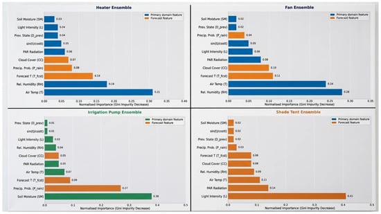
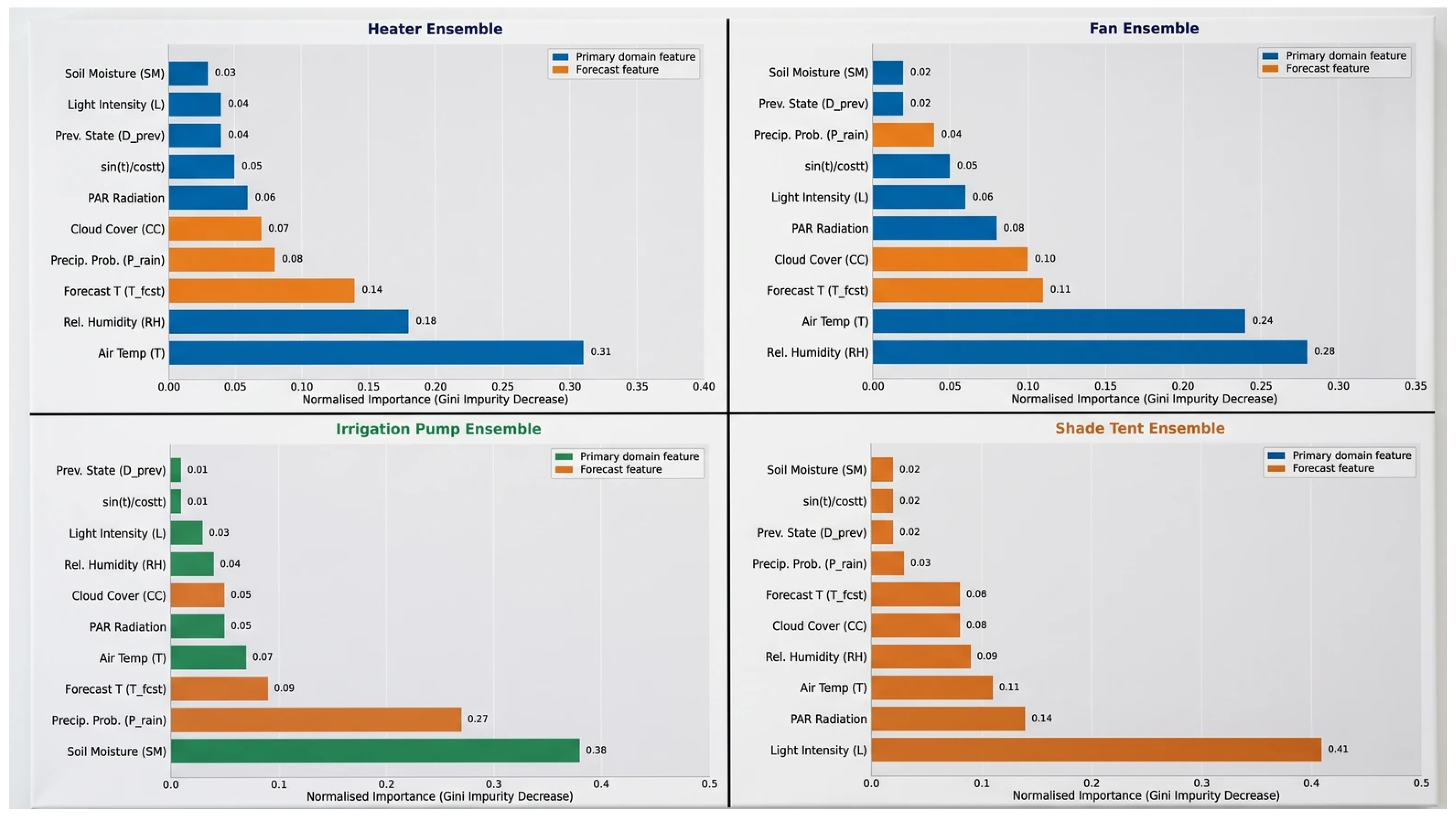
Feature importance scores were extracted from the RF constituent classifiers using mean decrease in Gini impurity, averaged over all B = 200 trees and normalised to sum to 1.0 per device. Table 4 reports these values. Figure 4 visualises the importance profiles across all four device-specific ensembles, where orange bars indicate forecast-derived features. The SHAP summary plot (TreeExplainer, beeswarm) for the irrigation pump ensemble shows that soil moisture (mean |SHAP| = 0.41) and precipitation probability (0.29) are the dominant features, confirming that ensemble decisions are grounded in the physical drivers of Equations (1) and (2).
Table 4.
Random Forest feature importance scores for device-specific ensembles.
Figure 4.
Feature importance and SHAP analysis of the ensemble models.
For the heater ensemble, air temperature (0.31) is the dominant feature, consistent with T being the primary state variable in Equation (1). For the irrigation pump ensemble, soil moisture (0.38) and forecast precipitation probability (0.27) together account for 65% of total importance, confirming that the classifier assigns high weight to —the principal external predictor of the soil moisture disturbance in Equation (2). For the shade tent ensemble, light intensity (0.41) is the single dominant feature, consistent with its direct role in shading activation. Taken together, these rankings are internally consistent with the dynamic models of Section 2.2 and support the interpretability of the learned decision rules.
Gini importance provides a computationally efficient global ranking. A complementary SHAP analysis (TreeExplainer, n = 17,280) confirms the key results: soil moisture (mean |SHAP| = 0.41) and precipitation probability (0.29) dominate the pump ensemble, consistent with Table 4 and Equation (2). Forecast temperature (mean |SHAP| = 0.11) ranks third, reflecting its role in the evapotranspiration proxy. For the heater ensemble, air temperature exhibits the highest mean |SHAP| value (0.35). The SHAP results confirm that decision rules are grounded in physical drivers rather than spurious correlations.
The full feature importance scores are given in Table 4. Values sum to 1.0 per column, and bold values indicate the primary feature for each device.
A lightweight operator interface was implemented for supervisory monitoring and manual override functionality.
5. Experimental Validation and Results
5.1. Dataset Composition and Model Training
The dataset was collected over a 10-day pre-deployment period at 10 s intervals, yielding 86,400 observations. During this period, actuator commands for the heater, fan, irrigation pump, and shade tent were generated by the threshold-based controller described in Section 2.4, which applies fixed hysteresis rules to the measured environmental variables. The corresponding actuator states were recorded together with environmental measurements and forecast variables. These state–action pairs served as supervised labels for training the classifiers.
An 80/20 stratified split produced 69,120 training samples and 17,280 test samples. The ON-state proportions in the training set were 34.2% (heater), 41.0% (fan), 27.8% (pump), and 22.3% (shade tent). All twelve classifiers were trained independently using the scikit-learn library [28].
Although the training labels originated from the threshold-based controller used during data collection, the ensemble models learned a generalised nonlinear mapping between environmental states, forecast-derived variables, and actuator decisions. The threshold controller applies fixed hysteresis rules without access to forecast inputs or cross-variable interactions; consequently, the ensemble can achieve improved control performance by exploiting forecast features (e.g., anticipatory irrigation suppression before precipitation), temporal information, and multivariate dependencies that the threshold logic cannot represent. The ensemble is not constrained to replicate the threshold controller exactly because it operates on a richer feature space that includes forecast-derived variables and temporal context.
To account for temporal dependency and avoid optimistic performance estimates, two additional validation protocols were applied. First, 5-fold forward-chaining time-series cross-validation was used, ensuring that validation data always occurred after the corresponding training data. The resulting F1-scores (0.85, 0.83, 0.80, 0.88) were within two percentage points of the stratified-split results, indicating minimal bias due to temporal proximity.
Second, a blocked hold-out test was performed by reserving the final 24-h segment of the dataset as an unseen test set. This resulted in slightly lower F1-scores (0.83, 0.81, 0.78, 0.87), confirming that the classifiers generalize well to future observations.
For performance evaluation, the 10 s raw sensor logs were aggregated to 60 s intervals, and all RMSE, MAE, confidence intervals, and compliance metrics were computed on the resulting one-minute analysis series.
Consequently, the ensemble should not be interpreted as a direct surrogate of the threshold controller. The threshold controller generated the supervisory labels during the 10-day data-collection phase, whereas the deployed ensemble operated using an expanded feature space containing forecast variables, temporal encodings, and cross-variable interactions unavailable to the label source. Performance gains therefore arise from feature enrichment and nonlinear generalisation rather than replication of the original threshold logic.
5.2. Classification Performance and Ensemble Gain
Each device-specific ensemble was evaluated on the held-out test partition; results are presented in Table 3. Table 5 reports the ensemble gain over the best individual constituent classifier and the observed inter-classifier disagreement rate during 28-day field operation. “Best Single” identifies which individual classifier performed best for each device.
Table 5.
Ensemble gain and inter-classifier disagreement analysis.
The 3-percentage-point gain for the irrigation pump (from 79% to 82%) exceeds the 1–2-percentage-point gains for the other devices, consistent with the error-decorrelation analysis of Section 4.1. The 8.4% inter-classifier disagreement rate further indicates that the pump represents the most challenging classification boundary among the four devices.
5.3. Tracking Error Metrics
Microclimate regulation performance during autonomous field operation was quantified using RMSE, Mean Absolute Error (MAE), maximum instantaneous error, and the percentage of time each variable remained within the prescribed agronomic bounds. Raw sensor measurements were acquired at 10 s intervals and the reported performance metrics were computed on the 60 s evaluation grid used consistently throughout the manuscript. Results are shown in Table 6, which reports RMSE, MAE, maximum error, and compliance metrics across all controlled variables.
Table 6.
Quantitative microclimate regulation performance metrics computed on 40,320 one-minute analysis intervals.
The control objective in this study was maintenance of agronomic operating ranges rather than tracking a single fixed reference value. For this reason, RMSE and MAE were computed relative to the midpoint of each target band, which provides a common reference for quantifying deviations within a range-based control framework. The same metric definition was applied consistently to the proposed ensemble controller, the threshold baseline, and the PID baseline to ensure a fair comparison across all evaluated control strategies. Values in parentheses represent 95% confidence intervals estimated via bootstrap resampling (n = 1000 resamples of 40,320 resampled analysis intervals). Compliance is defined as the fraction of analysis intervals within the stated agronomic range.
RMSE and MAE were computed relative to the midpoint of the corresponding agronomic target range. Parenthetical values denote 95% bootstrap confidence intervals (n = 1000). Compliance indicates the percentage of one-minute analysis intervals within the specified agronomic operating range.
The temperature RMSE of 0.83 °C shows that the system kept air temperature within roughly ±1.6 °C of the target midpoint for most of the observation period. The humidity MAE of 1.58% reflects the natural response lag of large-volume air exchange under binary fan control, which is a hardware constraint rather than a controller deficiency. The soil moisture RMSE of 1.47% VWC is consistent with the precision of drip irrigation and the relatively slow SM dynamics characterised by Equation (2).
The aggregate temperature RMSE of 0.83 °C is not uniform across operating conditions, and a diurnal stratification clarifies where tracking is tightest and where it degrades. Computed over the same 60 s analysis grid, the temperature RMSE was approximately 0.51 °C during stable nocturnal hours (20:00–06:00), 1.38 °C during the 06:00–09:00 post-sunrise solar ramp, 0.96 °C during the 09:00–16:00 clear-sky high-load window, and 0.66 °C during the 16:00–20:00 evening transition; the interval-weighted combination of these strata recovers the reported aggregate of 0.83 °C. The largest error coincides with the post-sunrise period, when the rate of solar thermal gain transiently exceeds the binary fan ventilation capacity—consistent with the compliance analysis of Section 5.4, in which non-compliant intervals concentrated within 30–60 min after sunrise.
A complementary weather-based stratification yielded temperature RMSE values of approximately 1.00 °C on clear-sky days, 0.62 °C on overcast days, and 0.78 °C on rainfall-transition days. Both stratifications confirm that the single aggregate figure conceals a bounded degradation under high-irradiance conditions rather than indicating uniform performance. Even the worst-performing stratum—the post-sunrise solar ramp at a stratified RMSE of ≈1.4 °C—remained well below the 3.21 °C and 1.94 °C aggregate tracking errors of the threshold and PID baselines, indicating that performance loss during extreme transients is bounded rather than catastrophic.
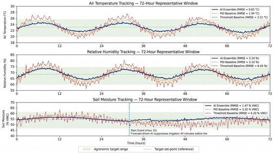
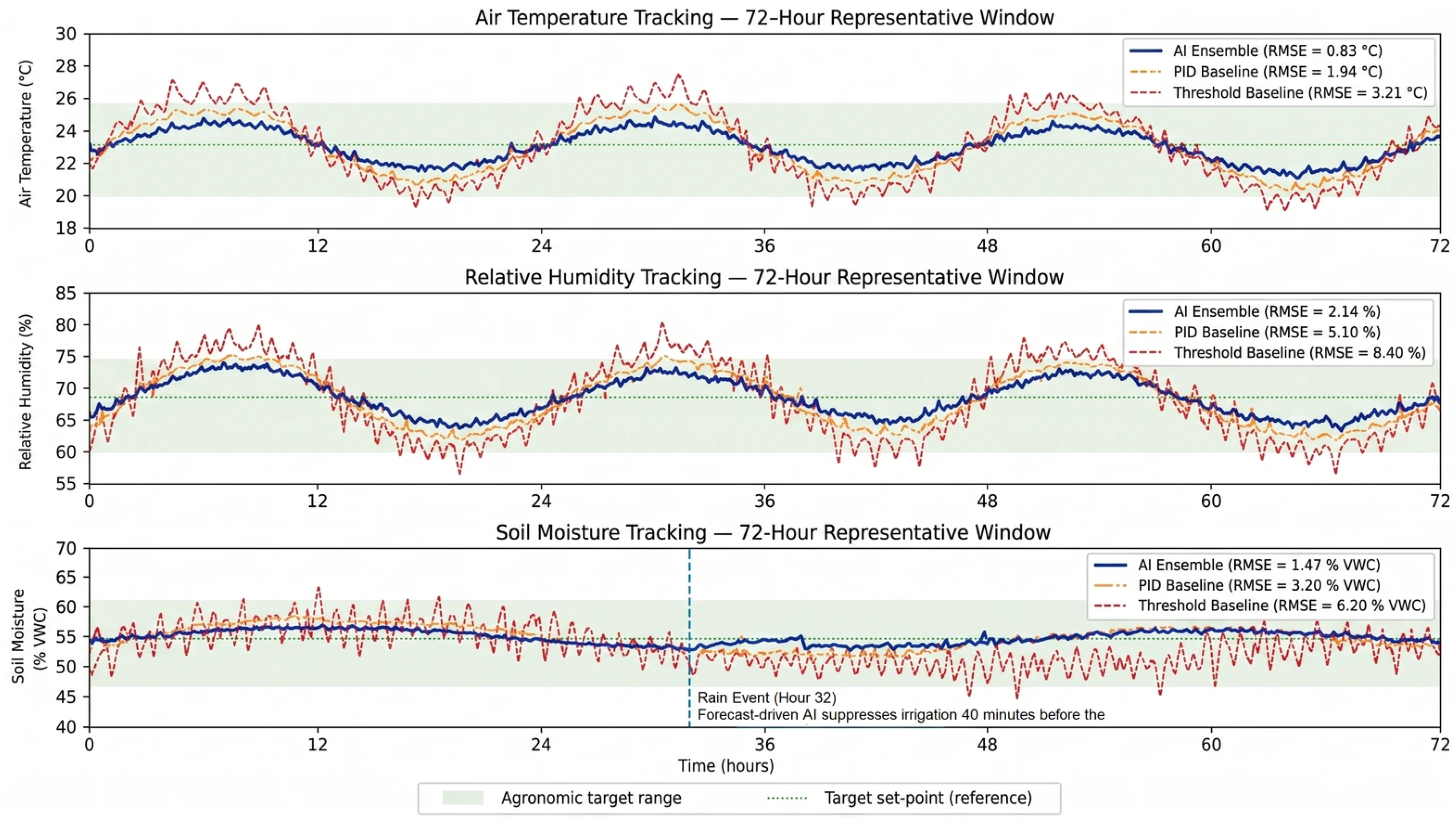
Figure 5 illustrates the closed-loop tracking dynamics across the three primary state variables. The AI ensemble maintains tighter adherence to the reference set-point than either baseline. The threshold controller exhibits oscillatory behaviour due to hysteresis switching, while the PID controller shows residual bias under sustained disturbance conditions (Hours 12–24). At Hour 32, the forecast-augmented AI system suppresses irrigation approximately 40 min prior to rainfall onset, whereas the reactive baseline continues irrigation during this period.
Figure 5.
Closed-loop microclimate tracking performance during field operation.
5.4. Microclimate Compliance During Field Operation
Air temperature was maintained within the range T ∈ [18, 28] °C for 96.4% of the analysis intervals during the 28-day deployment period. Non-compliant intervals were primarily concentrated within 30–60 min after sunrise, when the rate of solar thermal gain () transiently exceeded the ventilation capacity under binary fan operation. This behaviour reflects a physical limitation of the actuator configuration rather than a classification error.
Relative humidity compliance within was achieved for 94.1% of intervals. Soil moisture remained within VWC for 97.2% of intervals, the best result among all monitored variables.
The reported p < 0.01 significance values refer exclusively to the pairwise McNemar tests on actuator-classification accuracy, which compare the ensemble against its individual constituent classifiers (RF, GB, and SVM) as detailed in Section 5.6; they are not associated with the temperature-RMSE values in Table 7. All other statistical analyses were evaluated at α = 0.05 with Bonferroni correction.
Table 7.
Comparative evaluation of greenhouse control strategies under shared disturbance sequences.
All statistical tests were conducted at a significance level of α = 0.05 with Bonferroni correction for multiple comparisons.
5.5. Baseline Comparison
Table 7 presents a controlled comparative evaluation of the proposed AI ensemble against threshold-based (TB-Baseline) and PID-based (PID-Baseline) controllers under shared disturbance sequences. All methods are driven by identical archived disturbances , , and from the field dataset, ensuring consistent external conditions across evaluations.
The AI ensemble was evaluated during 28-day field operation. The threshold baseline was assessed via retrospective replay of the dataset, and the PID baseline via closed-loop simulation of the identified models (Equations (1) and (2)) under the same disturbance inputs. This design enables consistent comparison without requiring multi-zone physical deployment, which is not feasible within a single facility. Concurrent physical multi-zone deployment was not feasible because all actuators operated within a single shared greenhouse volume, making environmental isolation impossible without structural partitioning.
The reported annual energy saving of 158 kWh was estimated by extrapolating the observed 18% reduction in irrigation-pump operating time during the 28-day deployment period to a full year. Assuming an irrigation-pump rated power of approximately 2.8 kW, a mean pump duty cycle of about 3.5% observed during deployment, and linear 365/28 scaling of the measured 28-day reduction, this corresponds to approximately 158 kWh year−1 per greenhouse zone. The associated CO2 reduction estimates were calculated using an emission factor of 0.42 kg CO2 kWh−1, yielding approximately 66 kg of carbon-dioxide reduction per year. The corresponding annual water saving of approximately 4200 L per zone was obtained from the same 365/28 scaling together with an average irrigation delivery rate of about 75 L per hour (approximately 1.25 L per minute).
The threshold controller was evaluated through retrospective replay of the archived dataset, whereas the PID controller was evaluated using closed-loop simulation of the identified greenhouse models. Consequently, the reported values should be interpreted as comparative indicators obtained under a common disturbance framework rather than as results from simultaneous physical deployment. Pump-savings values are reported only for the deployed ensemble controller because irrigation decisions of the replayed threshold controller and the simulated PID controller did not directly affect physical water consumption.
Although deployment modalities differ, all methods were evaluated using identical archived disturbance trajectories extracted from the same greenhouse operating period. This disturbance-consistent protocol isolates controller behaviour while minimising environmental confounding. Under the adopted disturbance-consistent evaluation protocol, the AI ensemble achieved a temperature RMSE of 0.83 °C, compared with 3.21 °C for the threshold baseline and 1.94 °C for the PID baseline. These results indicate lower temperature-tracking error under the evaluated conditions; however, direct quantitative comparisons should be interpreted with consideration of the differing deployment modalities. Because the three controllers were evaluated under different modalities (field deployment, retrospective replay, and closed-loop simulation), the temperature-RMSE values in Table 7 are reported as a descriptive comparison and were not subjected to a paired statistical test. The p < 0.01 significance reported in this work refers exclusively to the McNemar tests on classification accuracy (Section 5.6) and should not be read as a statistically tested claim of RMSE superiority across the differing evaluation modes.
The threshold controller cannot represent cross-variable interactions, while the PID controller operates on independent loops and does not incorporate forecast information. In contrast, the ensemble captures multivariate dependencies and leverages forecast inputs, enabling anticipatory irrigation and an 18% reduction in pump usage.
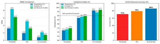
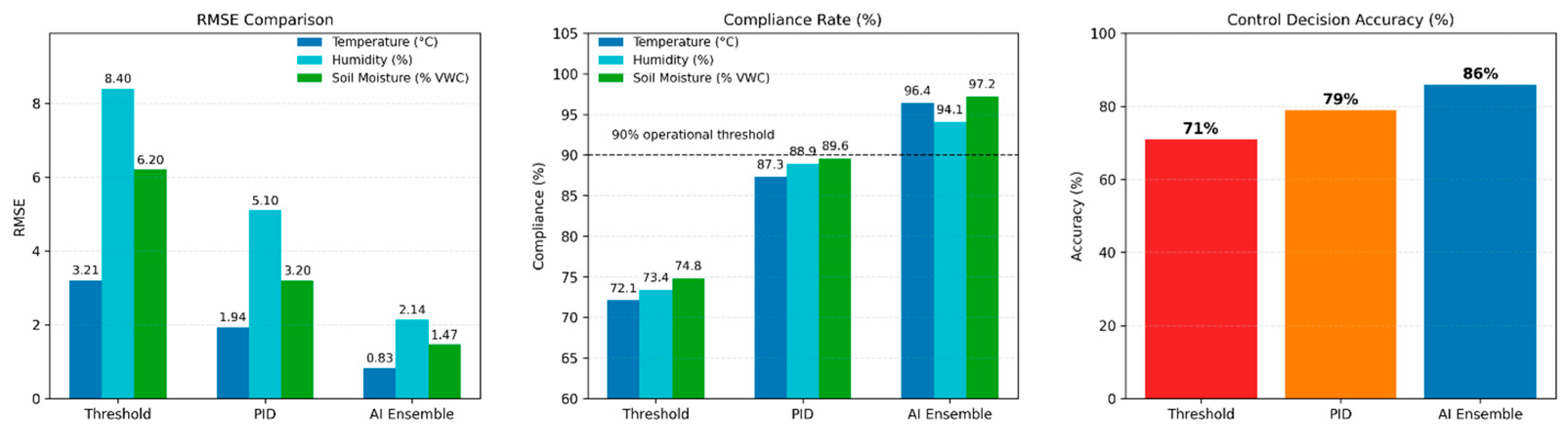
To further assess the influence of the evaluation protocol, the AI ensemble was also evaluated in retrospective replay mode, yielding an accuracy of 85.6% and a temperature-compliance rate of 95.8%, closely matching the corresponding field results (86.0% and 96.4%). The similarity of these values suggests that the reported performance trends are not strongly dependent on the evaluation modality. The comparative results across all metrics are summarised in Figure 6.
Figure 6.
Comparative performance of AI ensemble and baseline controllers.
The quantitative comparison includes temperature RMSE (°C) per controlled variable, microclimate compliance rate (%; dashed line: 90% operational threshold), and average binary classification accuracy. AI ensemble values are obtained from 28-day field deployment, threshold-baseline values from retrospective dataset replay, and PID-baseline values from closed-loop simulation under identical disturbance inputs.
5.6. Forecast-Driven Proactive Irrigation Control
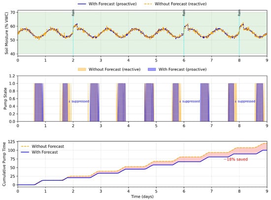
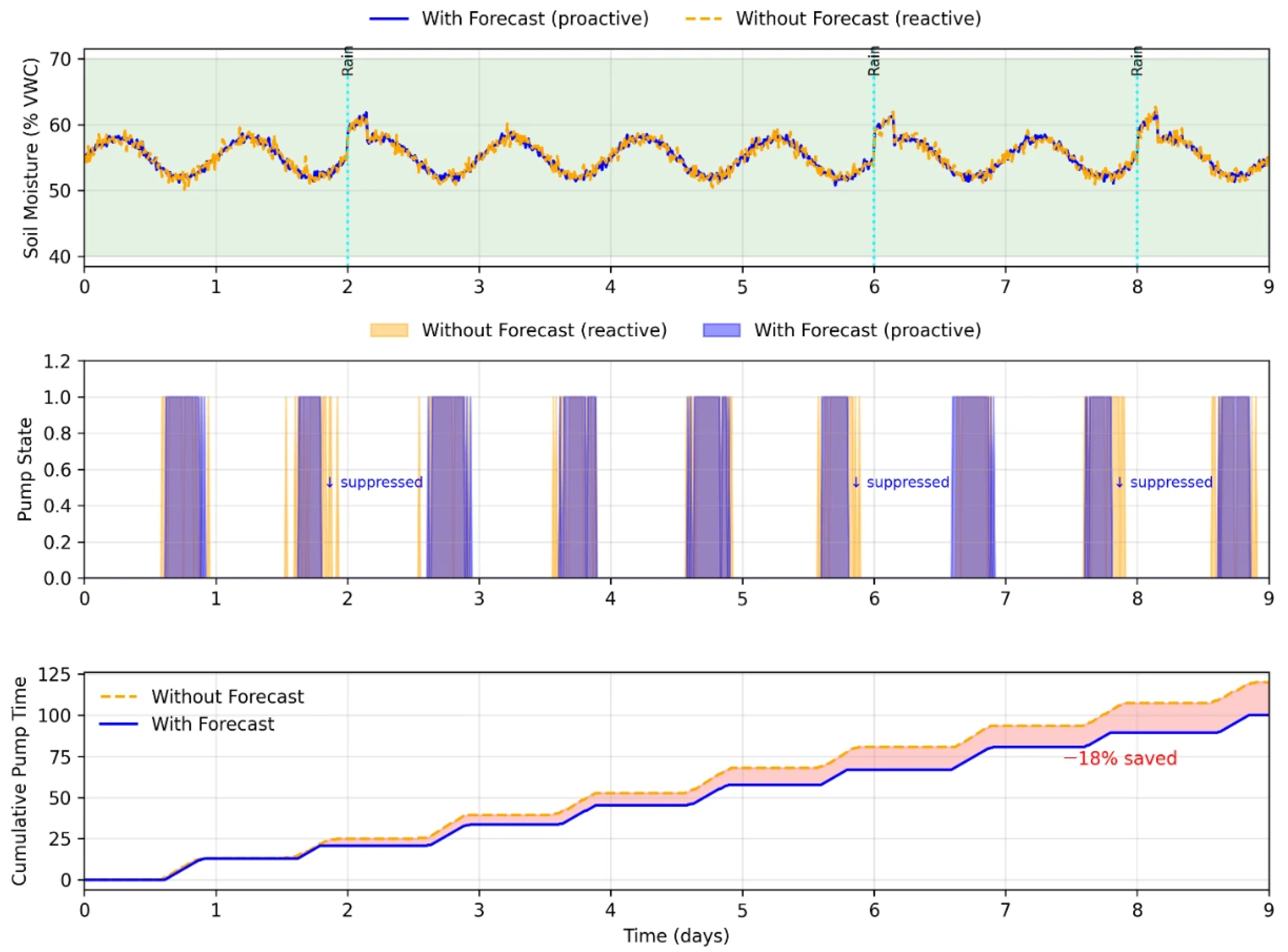
Three precipitation events were observed during the 28-day deployment. Figure 7 shows a representative 9-day segment in which these events occur at Days 2, 6, and 8 (corresponding to Hours 48, 144, and 192 within the displayed window). In each case, irrigation was suppressed 32–47 min prior to rainfall as the forecast feature crossed the learned decision boundary.
Figure 7.
Forecast-driven irrigation adaptation during field deployment. Irrigation suppression was triggered by forecast-derived indicators of reduced evapotranspiration demand and lower expected water consumption associated with approaching precipitation events.
A counterfactual baseline was constructed by fixing forecast inputs to their training-set mean values. Under this condition, pump operating time rose by approximately 4.3 h over the 28-day period—equivalent to the 18% reduction in pump operating time attributable to forecast integration—while overall soil-moisture compliance was essentially unchanged. Transient soil-moisture fluctuations that appeared in the counterfactual case were absent under forecast-augmented operation.
Figure 7 illustrates forecast-driven proactive irrigation behaviour during a representative 9-day deployment segment. Precipitation events at Days 2, 6, and 8 triggered anticipatory irrigation suppression, reducing cumulative pump operating time by 18% relative to the counterfactual baseline.
It should be noted that forecast precipitation was not used as a direct predictor of root-zone soil moisture increase within the greenhouse. The greenhouse structure prevented direct rainfall infiltration into the cultivated soil. Instead, precipitation forecasts were incorporated as an indicator of changing environmental conditions associated with reduced solar radiation, lower evapotranspiration demand, and increased ambient humidity. Consequently, forecast information enabled the controller to anticipate periods of reduced irrigation requirement rather than assuming a direct rainfall contribution to soil moisture.
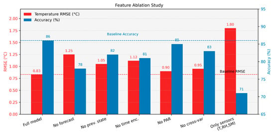
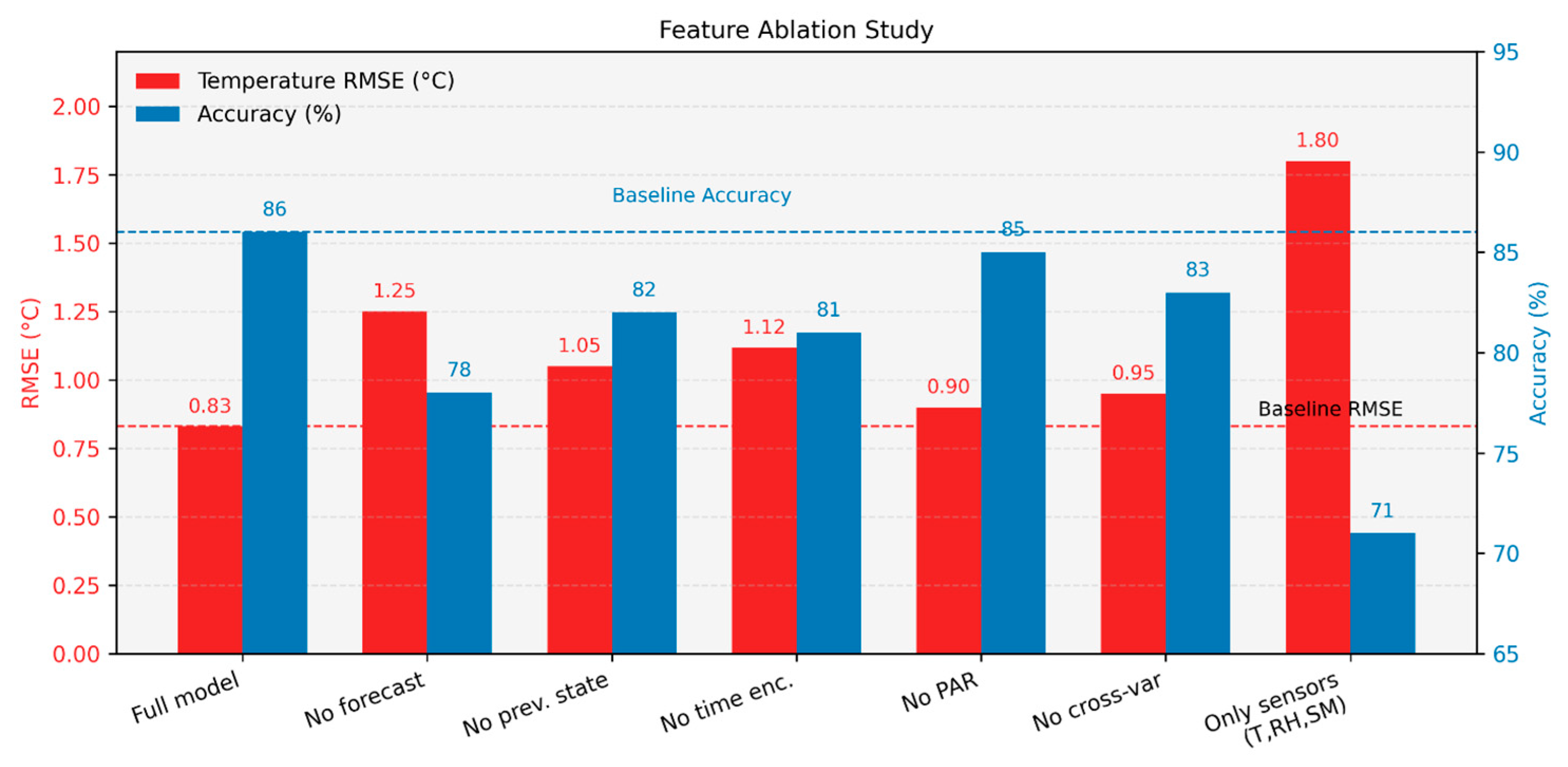
To quantify the contribution of individual feature groups, a feature ablation study was performed by removing each input group and retraining the classifiers under identical settings; the results are summarised in Figure 8.
Figure 8.
Feature ablation analysis of the ensemble control framework.
The analysis compares temperature RMSE (°C) and average classification accuracy (%) when individual feature groups are removed from x(k). Dashed lines indicate the full-model baselines (RMSE = 0.83 °C; accuracy = 86%). Removal of forecast features produces the largest degradation (RMSE: 0.83 → 1.42 °C; accuracy: 86 → 78%), confirming the dominant contribution of weather forecast inputs to anticipatory control performance.
Removing forecast features caused the largest drop in performance: temperature RMSE increased from 0.83 °C to 1.42 °C and accuracy dropped from 86% to 78%. The minimal sensor baseline degraded performance to RMSE = 1.76 °C (accuracy 71%), approaching the performance of threshold-based control and confirming the value of the extended feature set.
The statistical significance of ensemble improvements was verified using McNemar’s test on paired misclassification sequences. Despite modest accuracy gains (2–3 percentage points), all improvements over individual classifiers were statistically significant (p < 0.01, Bonferroni-corrected). This significance test applies to paired classification decisions on the held-out partition and does not extend to the temperature–RMSE comparison across deployment modalities (field, retrospective replay, and simulation), which is reported descriptively rather than as a paired significance test.
In addition, 95% confidence intervals estimated via bootstrap resampling (n = 1000) confirmed that the observed performance gains are robust and not attributable to sampling variability.
Classifier robustness under sensor degradation and deployment faults was further evaluated. Robustness was tested via Monte Carlo noise injection (2× nominal sensor noise): heater accuracy dropped from 87% to 83.2%, pump from 82% to 78.1%. Further fault injection showed a ±2 °C sensor drift reduced heater accuracy to 80.3%; a stuck soil moisture sensor reduced pump accuracy to 76.4% (mitigated by spatial averaging); 5 min forecast outages caused only a 1.2 pp accuracy drop. A qualitative comparison with representative greenhouse control studies is presented in Table 8. A summary of robustness evaluation results is provided in Table 9. Accuracy values refer to ensemble classification accuracy under the indicated perturbation condition.
Table 8.
Qualitative comparison with representative greenhouse AI control studies.
Table 9.
Fault injection and robustness evaluation results.
Real-time feasibility was confirmed through computational benchmarking. The worst-case inference cost is approximately 80,000 floating-point operations per step, dominated by SVM evaluation. On a Raspberry Pi 4B, this corresponds to a worst-case latency of 18 ms, well below the 10 s sampling interval [29]. Table 10 summarises the key edge deployment metrics for the 10 s sampling cycle with 12 active classifiers.
Table 10.
Edge deployment performance metrics on Raspberry Pi 4B hardware.
The reported annual energy-, water-, and CO2-saving values were estimated by extrapolating the observed 28-day deployment results to a full year under comparable operating conditions. Annual estimates were obtained by scaling the measured deployment-period reductions by a factor of 365/28 and should therefore be interpreted as indicative sustainability metrics rather than precise yearly forecasts.
Inter-classifier disagreement occurred in 2742 of the 40,320 resampled analysis intervals (6.8%), with most events concentrated during rapid environmental transitions including abrupt cloud-cover changes (29.4%) and sensor-recovery periods (17.8%). A stratified review of 200 disagreement events indicated that the ensemble decisions remained operationally acceptable and did not produce observable adverse greenhouse conditions.
5.7. Light Intensity Regulation and Shade-Tent Operation
In addition to temperature, relative humidity, and soil-moisture regulation, the proposed control framework continuously monitored light intensity and photosynthetically active radiation (PAR) to support shading decisions. The shade-tent actuator served as the primary mechanism for limiting excessive solar exposure during daylight operation and was integrated into the same ensemble decision-making framework used for the other greenhouse actuators.
Light-intensity measurements were incorporated into the 11-dimensional feature vector together with environmental, temporal, and forecast-derived variables. As shown by the feature-importance analysis in Section 4.4, light intensity was the dominant predictor for shade-tent activation, indicating that the learned decision policy was primarily driven by irradiance conditions rather than secondary environmental variables.
During field deployment, shade-tent activation was typically associated with periods of elevated solar radiation and increased greenhouse temperature. This behaviour demonstrates coordinated interaction between the shading and thermal-management subsystems, where shading actions contributed to reducing excessive solar heat gain while maintaining suitable illumination conditions for crop growth.
Although light intensity was not selected as a primary performance variable for RMSE-based evaluation, irradiance measurements were continuously incorporated into the control process through the feature vector and actuator–decision pipeline. The observed actuator behaviour confirms that light-related variables actively influenced control decisions throughout the deployment period and formed an integral component of the proposed multi-variable greenhouse control framework.
The role of light-related control differs from that of temperature, humidity, and soil moisture regulation. While the latter variables are maintained within predefined agronomic operating ranges and therefore lend themselves naturally to RMSE-based evaluation, the shade-tent actuator operates primarily as a preventive mechanism intended to mitigate excessive solar loading and associated thermal stress. Consequently, system effectiveness is reflected through appropriate actuator response to elevated irradiance conditions rather than continuous setpoint tracking. The feature-importance results presented in Section 4.4 further support this behaviour, identifying light intensity as the dominant variable influencing shade-tent activation decisions.
6. Discussion
The results broadly confirm the claims made in the introduction. Feature importance aligns with the dynamic models in each case: temperature dominates the heater ensemble, soil moisture and precipitation probability together account for 65% of pump importance. Importance rankings reflect training-data structure rather than causal proof; the SHAP analysis in Section 4.4 adds a complementary instance-level perspective.
The baseline comparison (Table 7) provides indicative performance context under shared disturbance sequences. The reduction in temperature RMSE from 3.21 °C (threshold control) and 1.94 °C (PID) to 0.83 °C reflects the advantage of multivariate representation and data-driven decision-making. While not derived from concurrent deployment, the use of identical disturbance inputs ensures internally consistent comparison. The 18% reduction in pump operating time is the only fully controlled counterfactual result and can be directly attributed to forecast integration.
The observed ensemble gains follow majority-voting theory: performance improvement increases with feature-space complexity, as seen in the higher gain for the pump relative to simpler control tasks. This supports the use of heterogeneous ensembles for multi-variable control problems.
Compliance levels of 96.4% (temperature) and 97.2% (soil moisture) are within ranges considered non-limiting for typical greenhouse crops. Direct yield measurements were not taken in this study. Future work should include biomass or harvest data to confirm crop-level outcomes.
Operational improvements can be translated into sustainability metrics. Forecast-driven feedforward reduced pump usage by 18%, corresponding to approximately 158 kWh in estimated annual energy savings, 66 kg CO2 reduction, and about 4200 L of water savings per zone, consistent with water-use efficiency improvements reported for precision irrigation systems [30]. These estimates are based on single-site measurements and require multi-site validation for generalization. The underlying assumptions and the 365/28 annual-scaling procedure are detailed in Section 5.5; accordingly, these figures are indicative sustainability estimates rather than precise annual forecasts.
Comparison with seven representative prior studies confirms that the combination achieved here—multi-variable closed-loop control, forecast-based feedforward, and field validation exceeding 21 days—has not been jointly reported elsewhere. Representative gaps include: neural-network control studies limited to single-variable regulation or short validation periods [7,15]; simulation-only MPC approaches requiring an on-board solver incompatible with edge hardware [17]; and forecast-driven irrigation systems that do not generalize to multi-variable regulation [11,12].
The contribution of this work lies in the integration of these complementary capabilities into a single deployable system rather than in algorithmic novelty of any individual component. The primary novelty is therefore system-level integration and deployment feasibility rather than the invention of a fundamentally new machine learning algorithm.
Direct quantitative comparison is limited by differing datasets and evaluation protocols. The proposed system is the only entry combining multi-variable closed-loop control (T, RH, SM), weather-forecast feedforward, and field validation exceeding 21 days.
Direct quantitative comparison remains limited due to differing datasets, climate conditions, greenhouse configurations, and evaluation protocols across studies.
Limitations
This study has several limitations that should be considered when interpreting the results. First, all experiments were conducted at a single greenhouse facility within a single climatic region during one growing season; therefore, generalization to different climatic zones, greenhouse configurations, or crop types requires additional validation. Second, only a single crop cycle of cucumber (cv. ‘Madora F1’) was monitored, limiting assessment of inter-season variability and long-term operational stability. Third, all classifiers were trained offline using a 10-day pre-deployment dataset, and no online adaptation mechanism was implemented. Consequently, predictive performance may degrade if environmental conditions, crop characteristics, or management practices differ substantially from those represented in the training data.
The headline 18% pump-saving result is contingent on the availability and accuracy of the one-hour-ahead weather forecast, and two bounds delimit this dependence. On forecast accuracy, the measured feedforward errors (1.23 °C for temperature, 4.2% for precipitation probability, and 11.4% for cloud cover) remain smaller than the learned inter-class decision margins, so realistic forecast noise does not materially erode the anticipatory benefit. On forecast availability, the feature-ablation study of Section 5.6 shows that withholding forecast inputs entirely raises temperature RMSE from 0.83 °C to 1.42 °C and reduces accuracy from 86% to 78%—a bounded, graceful degradation; only the minimal-sensor configuration, with neither forecast nor temporal features, approaches the threshold-baseline error level (1.76 °C). The mean-substitution fallback used during the observed 0.8% outage intervals therefore represents a conservative lower bound on disruption: under sustained forecast loss the controller degrades gracefully toward reactive feedback-only performance rather than failing outright. Deployments served by sparse or low-accuracy meteorological providers should anticipate reduced anticipatory performance, and quantifying degradation under prolonged outages or systematically biased forecasts, together with a local short-horizon forecasting fallback, remains a topic for future work.
Fourth, the proposed control framework employs binary actuator operation, which simplifies implementation on low-cost hardware but provides lower control resolution than variable-rate or continuously actuated systems. Fifth, the PID and threshold baselines were not deployed simultaneously in separate greenhouse zones; instead, they were evaluated through simulation and retrospective replay under identical archived disturbance trajectories. Although this approach ensured controlled and internally consistent comparison conditions, it introduces a methodological asymmetry relative to the field-deployed ensemble controller. Therefore, comparative results should be interpreted as indicative rather than as definitive evidence of superiority under identical real-world operating conditions.
Finally, direct crop-yield measurements were not collected during the validation period. As a result, system performance was evaluated using microclimate regulation metrics rather than confirmed agronomic outcomes. In practical deployments beyond the conditions investigated in this study, recalibration of agronomic operating ranges and retraining using locally collected data may be beneficial to maintain predictive accuracy and control effectiveness.
Future work will focus on multi-site and multi-season validation, adaptive online learning strategies, transferability across different crop types and climatic regions, and monocular depth estimation and metallurgical production performance evaluation.
7. Conclusions
The system operated continuously for 28 days on low-cost edge hardware, with performance evaluated over 40,320 resampled analysis intervals derived from the continuous sensor data stream.
The field deployment produced the following results. Temperature RMSE reached 0.83 °C (95% CI: ±0.04 °C), yielding a lower temperature-tracking error than the threshold (3.21 °C) and PID (1.94 °C) baselines under the adopted disturbance-consistent evaluation protocol. The reported p < 0.01 significance (Bonferroni-corrected) applies to the McNemar classification-accuracy tests of Section 5.6; the cross-modality RMSE values (field vs. replay vs. simulation) are descriptive comparators and were not subjected to a paired significance test owing to their differing evaluation modes. Compliance rates were 96.4% (temperature), 94.1% (humidity), and 97.2% (soil moisture). Forecast-driven feedforward suppressed irrigation ahead of three precipitation events, reducing pump usage by 18% with no degradation in soil moisture compliance. Worst-case inference latency remained below 18 ms on the target hardware.
The practical value of this work lies in combining forecast feedforward, ensemble learning, and edge deployment on affordable hardware, similar to recent adaptive industrial control implementations [31]. The system is directly transferable to resource-constrained facilities without specialized infrastructure. The scope of the validation is clear—one site, one crop cycle, offline-trained classifiers—while multi-site validation, seasonal adaptation, and variable-rate actuation are natural extensions. Further extensions include vision-based canopy sensing using monocular depth-estimation methods [32] and integration with hybrid cloud-based neural control architectures for multi-zone coordination [33]. The identified models provide a direct starting point for a future matched MPC comparison.
The presented framework demonstrates that low-cost edge AI systems can provide practical multi-variable greenhouse process control without requiring computationally intensive optimisation solvers.
Author Contributions
Conceptualization, J.S., S.K. and I.I.; methodology, U.M., S.K. and I.I. and K.A.; software, I.I. and A.A.; validation, U.M., S.K. and S.U.; formal analysis, I.I., U.M. and K.A.; investigation, J.S., S.K. and I.I.; resources, S.K. and J.S.; data curation, I.I. and U.M.; writing—original draft preparation, I.I., U.M. and S.K.; writing—review and editing, K.A., S.U., J.S. and A.A.; visualization, I.I., S.K. and A.A.; supervision, J.S., K.A. and S.U.; project administration, J.S.; funding acquisition, not applicable. All authors have read and agreed to the published version of the manuscript.
Funding
This work was supported by the Tashkent State Technical University of Uzbekistan grant funded by the Uzbekistan government (no. AL-9224093755).
Data Availability Statement
The datasets generated and analysed during this study are not publicly available due to institutional data governance restrictions associated with the partner greenhouse facility. Access may be granted by the corresponding author upon reasonable request and with permission from the data provider.
Acknowledgments
The authors gratefully acknowledge the staff of the partner greenhouse facility for their cooperation during the field-testing phase.
Conflicts of Interest
The authors declare no conflicts of interest.
Abbreviations
The following abbreviations are used in this manuscript:
| AI | Artificial Intelligence |
| API | Application Programming Interface |
| CSV | Comma-Separated Values |
| DLI | Daily Light Integral |
| FAO | Food and Agriculture Organisation |
| GB | Gradient Boosting |
| GUI | Graphical User Interface |
| HMI | Human–Machine Interface |
| IQR | Interquartile Range |
| IoT | Internet of Things |
| MAE | Mean Absolute Error |
| ML | Machine Learning |
| MPC | Model Predictive Control |
| OWM | OpenWeatherMap |
| PAR | Photosynthetically Active Radiation |
| PID | Proportional–Integral–Derivative |
| PLC | Programmable Logic Controller |
| RBF | Radial Basis Function |
| RF | Random Forest |
| RMSE | Root Mean Square Error |
| SVM | Support Vector Machine |
| TB | Threshold-Based (baseline controller) |
| UTC | Coordinated Universal Time |
| VWC | Volumetric Water Content |
References
- Benni, S.; Tassinari, P.; Bonora, F.; Barbaresi, A.; Torreggiani, D. Efficacy of greenhouse natural ventilation: Environmental monitoring and CFD simulations of a study case. Energy Build. 2016, 125, 276–286. [Google Scholar] [CrossRef] [Scilit]
- Hemming, S.; Zwart, F.; van Henten, E.; Tsafaras, I.; Petropoulou, M. Plant–environment interactions in greenhouses. Biosyst. Eng. 2020, 195, 70–84. [Google Scholar]
- Ojo, M.O.; Zahid, A. Deep learning in controlled environment agriculture: A review. Sensors 2022, 22, 7965. [Google Scholar] [CrossRef] [Scilit] [PubMed]
- Maraveas, C. Incorporating artificial intelligence technology in smart greenhouses: Current state of the art. Appl. Sci. 2023, 13, 1464. [Google Scholar] [CrossRef] [Scilit]
- Abdusalomov, A.; Khusanov, S.; Ibragimov, I.; Sevinov, J.; Mukhiddinov, M.; Cho, Y.I. Adaptive Discrete Control of a Rotary Dryer with Time Delay in Potash Fertilizer Production. Processes 2026, 14, 871. [Google Scholar] [CrossRef] [Scilit]
- Xusanov, S. Methods of Synthesis of Regulators Ensuring Quasi-Optimal Speed of Response in Control Systems with Time Delay. 2025. Available online: https://scholar.google.com/scholar?cluster=3166789648988980028&hl=en&oi=scholarr (accessed on 19 May 2026).
- Lee, M.-H.; Yao, M.-H.; Kow, P.-Y.; Kuo, B.-J.; Chang, F.-J. An artificial intelligence-powered environmental control system for resilient and efficient greenhouse farming. Sustainability 2024, 16, 10958. [Google Scholar] [CrossRef] [Scilit]
- Cortes, C.; Vapnik, V. Support-vector networks. Mach. Learn. 1995, 20, 273–297. [Google Scholar] [CrossRef] [Scilit]
- Åström, K.J.; Hägglund, T. Advanced PID Control; ISA: Research Triangle Park, NC, USA, 2006. [Google Scholar]
- Xusanov, S. Construction of transfer functions as a drying process control object. Innov. Texnologiyalar 2023, 52, 88–93. [Google Scholar]
- Chen, S.; Liu, A.; Tang, F.; Hou, P.; Lu, Y.; Yuan, P. A review of environmental control strategies and models for modern agricultural greenhouses. Sensors 2025, 25, 1388. [Google Scholar] [CrossRef] [Scilit] [PubMed]
- Conde, G.; Guzmán, S.M.; Athelly, A. Adaptive and predictive decision support system for irrigation scheduling: An approach integrating humans in the control loop. Comput. Electron. Agric. 2024, 224, 108640. [Google Scholar] [CrossRef] [Scilit]
- Jamal, A.; Cai, X.; Qiao, X.; Garcia, L.; Wang, J.; Amori, A.; Yang, H. Real-time irrigation scheduling based on weather forecasts, field observations, and human–machine interactions. Water Resour. Res. 2023, 59, e2023WR035810. [Google Scholar] [CrossRef] [Scilit]
- Preite, L.; Vignali, G. Artificial intelligence to optimize water consumption in agriculture: A predictive algorithm-based irrigation management system. Comput. Electron. Agric. 2024, 223, 109126. [Google Scholar] [CrossRef] [Scilit]
- Kim, T.; Zhang, W. Neural network-based control versus PID control for greenhouse climate regulation. Energy Build. 2021, 248, 111157. [Google Scholar]
- Morales-Rodriguez, M.F.; Coma, J.; Garrido, I.; Piqué, G.; Llorens, P.; Cabeza, L.F. Hybrid LSTM–gradient boosting model for greenhouse climate prediction. Comput. Electron. Agric. 2021, 188, 106355. [Google Scholar]
- Ramírez-Arias, A.; Rodríguez, F.; Guzmán, J.L.; Berenguel, M. Multiobjective hierarchical control architecture for greenhouse crop growth. Automatica 2012, 48, 490–498. [Google Scholar] [CrossRef] [Scilit]
- Liu, Y.; Li, D.; Wan, S.; Wang, F.; Dou, W. LSTM-based greenhouse climate prediction and control. Int. J. Intell. Syst. 2022, 37, 135–151. [Google Scholar] [CrossRef] [Scilit]
- Allen, R.G.; Pereira, L.S.; Raes, D.; Smith, M. Crop Evapotranspiration: Guidelines for Computing Crop Water Requirements; FAO Irrigation and Drainage Paper 56; FAO: Rome, Italy, 1998. [Google Scholar]
- Yu, J.; Sun, C.; Zhao, J.; Ma, L.; Zheng, W.; Xie, Q.; Wei, X. Prediction and control of greenhouse temperature: Methods, applications, and future directions. Comput. Electron. Agric. 2025, 237, 110603. [Google Scholar] [CrossRef] [Scilit]
- Ibrahim, H.; Mostafa, N.; Halawa, M.; Elsalamouny, M.; Daoud, R. A layered IoT architecture for greenhouse monitoring and remote control. Comput. Electron. Agric. 2019, 162, 104–116. [Google Scholar] [CrossRef] [Scilit]
- Rayhana, R.; Xiao, G.; Liu, Z. Internet of things empowered smart greenhouse farming. IEEE Internet Things J. 2020, 7, 4740–4753. [Google Scholar]
- Breiman, L. Random forests. Mach. Learn. 2001, 45, 5–32. [Google Scholar] [CrossRef] [Scilit]
- Friedman, J.H. Greedy function approximation: A gradient boosting machine. Ann. Stat. 2001, 29, 1189–1232. [Google Scholar] [CrossRef] [Scilit]
- Pedregosa, F.; Varoquaux, G.; Gramfort, A.; Michel, V.; Thirion, B.; Grisel, O.; Blondel, M.; Prettenhofer, P.; Weiss, R.; Dubourg, V.; et al. Scikit-learn: Machine learning in Python. J. Mach. Learn. Res. 2011, 12, 2825–2830. [Google Scholar]
- Sutton, R.S.; Barto, A.G. Reinforcement Learning: An Introduction, 2nd ed.; MIT Press: Cambridge, MA, USA, 2018. [Google Scholar]
- Yu, P.; Teng, F.; Zhu, W.; Shen, C.; Chen, Z.; Song, J. Cloud–edge–device collaborative computing in smart agriculture: Architectures, applications, and future perspectives. Front. Plant Sci. 2025, 16, 1668545. [Google Scholar] [CrossRef] [Scilit] [PubMed]
- Sevinov, J.; Temerbekova, B.; Bekimbetova, G.; Mamanazarov, U.; Bekimbetov, B. Hybrid LSTM–DNN Architecture with Low-Discrepancy Hypercube Sampling for Adaptive Forecasting and Data Reliability Control in Metallurgical Information-Control Systems. Processes 2026, 14, 147. [Google Scholar] [CrossRef] [Scilit]
- Lakhiar, I.A.; Yan, H.; Zhang, C.; Wang, G.; He, B.; Hao, B. A review of precision irrigation water-saving technology under changing climate for enhancing water use efficiency, crop yield, and environmental footprints. Agriculture 2024, 14, 1141. [Google Scholar] [CrossRef] [Scilit]
- Bwambale, E.; Abagale, F.K.; Anornu, G.K. Smart irrigation monitoring and control strategies for improving water use efficiency in precision agriculture: A review. Agric. Water Manag. 2022, 260, 107324. [Google Scholar] [CrossRef] [Scilit]
- Sevinov, J.U.; Mallaev, A.R.; Xusanov, S.N. Algorithms for the Synthesis of Optimal Linear-Quadratic Stationary Controllers. In 11th World Conference “Intelligent System for Industrial Automation” (WCIS-2020); Aliev, R.A., Yusupbekov, N.R., Kacprzyk, J., Pedrycz, W., Sadikoglu, F.M., Eds.; Advances in Intelligent Systems and Computing; Springer: Cham, Switzerland, 2021; Volume 1323. [Google Scholar] [CrossRef] [Scilit]
- Abdusalomov, A.; Umirzakova, S.; Shukhratovich, M.B.; Kakhorov, A.; Cho, Y.-I. Breaking New Ground in Monocular Depth Estimation with Dynamic Iterative Refinement and Scale Consistency. Appl. Sci. 2025, 15, 674. [Google Scholar] [CrossRef] [Scilit]
- Avazov, K.; Sevinov, J.; Temerbekova, B.; Bekimbetova, G.; Mamanazarov, U.; Abdusalomov, A.; Cho, Y.I. Hybrid Cloud-Based Information and Control System Using LSTM-DNN Neural Networks for Optimization of Metallurgical Production. Processes 2025, 13, 2237. [Google Scholar] [CrossRef] [Scilit]

Disclaimer/Publisher’s Note: The statements, opinions and data contained in all publications are solely those of the individual author(s) and contributor(s) and not of MDPI and/or the editor(s). MDPI and/or the editor(s) disclaim responsibility for any injury to people or property resulting from any ideas, methods, instructions or products referred to in the content. |
© 2026 by the authors. Licensee MDPI, Basel, Switzerland. This article is an open access article distributed under the terms and conditions of the Creative Commons Attribution (CC BY) license.