Joint Prediction of Reservoir-Fluid Identification and Water Saturation Based on YSF-Net: A Case Study for Youshashan Oilfield, Southwestern Qaidam Basin, China

Abstract

Accurate reservoir-fluid identification and water saturation prediction are essential for remaining-oil evaluation and water-flooding adjustment in heterogeneous oilfields. However, in the Youshashan Oilfield, southwestern Qaidam Basin, China, thin interbeds, strong reservoir heterogeneity, complex oil–water transitions, and inter-well logging-response differences make conventional single-task interpretation difficult. To address these problems, this study proposes a joint prediction method based on the Youshashan Fluid Prediction Network (YSF-Net) for six-class reservoir-fluid identification and continuous water saturation (S_w) prediction. A total of 200 wells were used and strictly divided by well into 140 training wells, 30 validation wells, and 30 independent test wells to avoid data leakage. Conventional logs were first processed through depth matching, outlier correction, robust standardization, and missing-value masking. Then, sliding-window logging sequences, regional stratigraphic embeddings, and reservoir-prior parameters, including shale volume, porosity, and permeability, were jointly input into the YSF-Net. The model uses a shared feature encoder with classification and regression branches to simultaneously identify oil layers, oil–water layers, water layers, and weakly, moderately, and strongly water-flooded layers, while predicting continuous S_w. A modified Simandoux-based physical consistency constraint was further introduced during training to improve the geological rationality of S_w prediction. Experimental results show that YSF-Net outperforms the CNN, BiLSTM, CNN-BiLSTM, and Transformer. It achieves an Accuracy of 0.926, Macro-F1 of 0.913, Macro-AUC of 0.968, S_w RMSE of 0.061, S_w MAE of 0.047, and S_w R² of 0.947. In direct cross-well testing without fine-tuning, YSF-Net obtains a Cross-well Accuracy of 0.918, Cross-well Macro-F1 of 0.904, and Cross-well S_w RMSE of 0.064. Ablation, transition-boundary, and typical well-interval analyses further demonstrate that regional constraints, reservoir-prior inputs, multi-task learning, and physical consistency improve class-boundary discrimination and S_w prediction reliability. The proposed method provides an accurate, consistent, and practical workflow for intelligent reservoir-fluid interpretation in heterogeneous reservoirs.

1. Introduction

Reservoir-fluid identification and water-saturation prediction are essential for well-log interpretation, reservoir evaluation, remaining-oil assessment, and water-flooding adjustment. In mature oilfields, the accurate discrimination of oil layers, oil–water layers, water layers, and water-flooded intervals directly affects perforation optimization, injection–production adjustment, and dynamic reservoir management. Recent studies have shown that machine-learning-based methods can improve water-saturation estimation, reservoir-parameter prediction, and well-log data reconstruction from conventional logging data [1,2,3]. However, in heterogeneous reservoirs, especially those with thin interbeds, complex facies transitions, and strong inter-well differences, fluid-state identification and water-saturation prediction remain difficult, because logging responses are often non-unique and strongly affected by lithology, pore structure, shale content, and development status.

Intelligent well-log interpretation has been widely developed in lithology, lithofacies, fluid identification, and petrophysical-parameter prediction. Early and representative studies demonstrated that supervised learning, hybrid machine-learning models, and deep-learning methods can improve lithofacies discrimination, permeability modeling, and logging-response feature extraction [4,5,6,7,8]. More recent studies further introduced explainable learning, hybrid convolutional–recurrent networks, saturation-determination methods, ensemble learning, deep neural networks, sediment-characterization models, and multi-head attention mechanisms for reservoir-fluid identification and water-saturation prediction [9,10,11,12,13,14,15]. These studies confirm that data-driven models can capture nonlinear relationships among conventional logs and reservoir properties more effectively than simple empirical interpretation.

With the continuous development of intelligent interpretation methods, researchers have further explored deep convolutional networks, fluvial-lithofacies models, deep neural networks from conventional logs, Bayesian-optimized classifiers, CNN-based single-well interpretation, hybrid CNN–SVM methods, residual vision transformers, 3D modeling, and graph-based clustering for complex reservoir characterization [16,17,18,19,20,21,22,23,24,25]. Meanwhile, water-saturation prediction has also evolved from conventional regression toward XGBoost, feature-ranking models, enhanced petrophysical evaluation, uncertainty quantification, integrated artificial-intelligence fluid identification, model-performance comparison, Multi-TransFKAN prediction, gas-saturation prediction, attention-based sequence modeling, and Bayesian uncertainty analysis [26,27,28,29,30,31,32,33,34,35,36,37]. These advances indicate that the field is moving from single-task prediction toward integrated interpretation, uncertainty awareness, cross-well generalization, and geological-constraint fusion.

Overall, previous studies have provided an important foundation for intelligent well-log interpretation, but several limitations remain for reservoirs with strong regional variation, stratigraphic differences, and complex fluid transitions, such as the Youshashan Oilfield. Most existing methods focus on lithology identification or single fluid discrimination, while joint modeling of fluid-state classification and continuous water-saturation prediction remains insufficient. In addition, regional stratigraphic differences, reservoir-prior parameters, and physical constraints are often not fully incorporated, which may lead to geologically inconsistent predictions. Their stability also needs improvement in thin layers, transition zones, and cross-well applications. Therefore, this study proposes YSF-Net to integrate regional constraints, reservoir-prior inputs, multi-task learning, and physical consistency constraints within a unified framework, aiming to improve the Accuracy, continuity, and engineering applicability of reservoir-fluid and S_w interpretation in complex intervals.

2. Theoretical and Formula System

2.1. Geological Setting, Well-Log Sequence Representation, and Reservoir-Prior Construction Under Regional Constraints

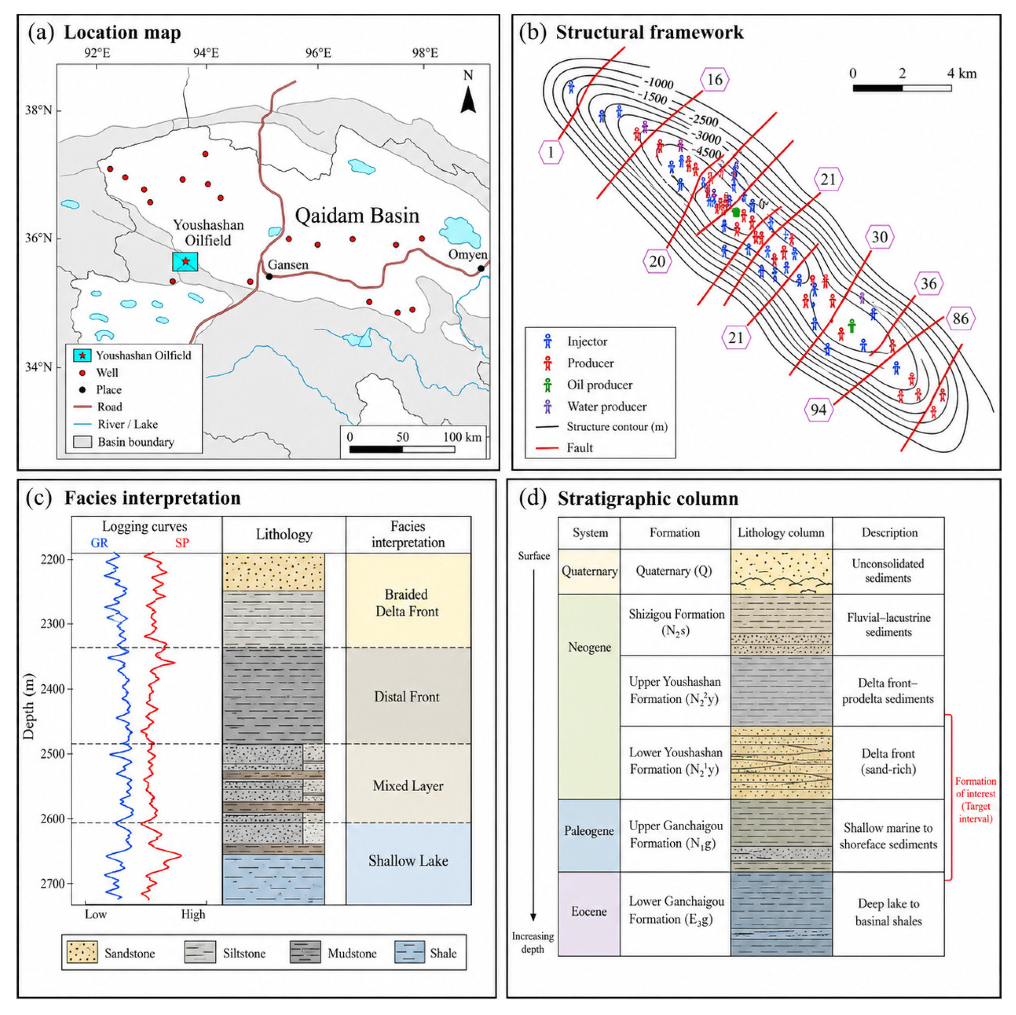
As shown in Figure 1, the Youshashan Oilfield is located in the southwestern Qaidam Basin, China, and represents a complex fault-block reservoir system. The study area is controlled by NE–SW-trending structures and multiple faults, resulting in strong fault-block segmentation and structural control on reservoir development and fluid distribution. The typical interval contains braided delta-front, distal front, mixed-layer, and shallow-lake deposits, with frequent sandstone, siltstone, mudstone, and shale interbeds, indicating strong vertical heterogeneity. The complete stratigraphic column includes the Quaternary, Neogene Shizigou Formation, Upper and Lower Youshashan formations, and Paleogene Upper and Lower Ganchaigou formations, with target reservoirs mainly developed in the Upper Youshashan, Lower Youshashan, and Upper Ganchaigou formations. These structural and sedimentary characteristics provide the geological basis for introducing regional constraints, stratigraphic information, and reservoir-prior parameters into YSF-Net.

Figure 1. Basic map of the location, structural background, and sedimentary interpretation of the Youshashan Oilfield.

Thin interbeds and rapid lateral facies changes cause clear zonal differences in logging responses among fluid states. Core–log calibration indicates that GR reflects shale content, density and acoustic transit time reflect pore structure and reservoir quality, and resistivity is closely related to hydrocarbon occurrence and water-bearing conditions. Therefore, multiple conventional logs were treated as multivariate depth sequences, and stratigraphic context was introduced to improve the recognition of thin beds, transition zones, and local anomalies. Reservoir heterogeneity was quantified using core-calibrated porosity and permeability. Type 1–3 delta-front clastic reservoirs show better quality, with a porosity of 7.0–22.8% and permeability of 0.30–185.0 mD. Type 4–5 distal front transitional reservoirs show lower and more dispersed properties, with a porosity of 5.6–18.4% and permeability of 0.12–63.5 mD. Type 6 mixed-deposition reservoirs have the strongest heterogeneity, with a porosity of 4.5–14.2% and permeability of 0.08–18.7 mD. The stronger variation in permeability further indicates the influence of thin interbeds, shale content, and pore–throat connectivity, supporting the use of reservoir-prior parameters and regional constraints in YSF-Net.

Assume that, after unified depth resampling, a given well interval contains $C$ logging curves and that the window length is $L$. Then, the input sample centered at the iii-th depth point is defined as:

$${\mathbf{X}}_i=\left[{\mathbf{x}}_{i-{\displaystyle \frac{L-1}{2}}},\dots ,{\mathbf{x}}_i,\dots ,{\mathbf{x}}_{i+{\displaystyle \frac{L-1}{2}}}\right]\in {\mathbb{R}}^{L\times C}$$

(1)

where ${\mathbf{x}}_i$ denotes the $C$-dimensional logging-response vector at the $i$-th depth point, and ${\mathbf{X}}_i$ denotes the logging window formed by the central depth point together with its upper and lower neighboring intervals. This representation preserves both the multi-log coupling at a single depth point and the continuous vertical variation in the stratigraphic sequence.

Considering that different wells, different logging suites, and different acquisition environments may introduce obvious amplitude drift and distributional differences, each logging curve is robustly standardized using statistical quantities derived from the training wells:

$${\tilde{x}}_{i,c}={\displaystyle \frac{x_{i,c}-\mathrm{M}\mathrm{e}\mathrm{d}\left(x_c\right)}{\mathrm{I}\mathrm{Q}\mathrm{R}\left(x_c\right)+\epsilon }}$$

(2)

where $x_{i,c}$ is the original value of the $c$-th log at the iii-th depth point, $\mathrm{M}\mathrm{e}\mathrm{d}\left(x_c\right)$ and $\mathrm{I}\mathrm{Q}\mathrm{R}\left(x_c\right)$ denote the median and interquartile range of this log in the training samples, respectively, and $\epsilon$ is a very small constant introduced to avoid division by zero. ${\tilde{x}}_{i,c}$ is the normalized logging value.

Before input construction, all well-log curves were uniformly preprocessed under the well-based data split. Depth resampling was performed to unify sampling intervals, and abnormal values caused by borehole enlargement, tool failure, or acquisition errors were identified using quality-control ranges and training-well statistics. Values beyond reasonable physical limits or deviating from the training-well median by more than five interquartile ranges were treated as anomalies. Isolated anomalies were corrected by interpolation, while continuous abnormal intervals were retained as missing segments and marked by a missing mask. To avoid data leakage, robust standardization was only conducted with training-well statistics. The median and interquartile range of each log were calculated from the training wells and then fixed for validation and test wells. Thus, no distributional information from unseen wells was introduced.

For missing values, short gaps were interpolated, whereas long gaps were filled with zeros after standardization and explicitly marked by the binary mask. The mask only indicates data availability and contains no fluid label or water-saturation information.

Because some well intervals contain missing curves or incomplete logging quality, a missing-mask matrix ${\mathbf{M}}_i\in \{0,1{\}}^{L\times C}$ is further defined to indicate the data validity of each position and each channel within the window. The normalized logs, missing mask, and stratigraphic regional embedding are jointly encoded into a unified input:

$${\mathbf{H}}_i=\mathrm{C}\mathrm{o}\mathrm{n}\mathrm{c}\mathrm{a}\mathrm{t}\left({\tilde{\mathbf{X}}}_i\odot {\mathbf{M}}_i,\hspace{0.17em}{\mathbf{M}}_i,\hspace{0.17em}{1}_L{\mathbf{e}}_{r\left(i\right)}^{\mathrm{\top }}\right)$$

(3)

where $\odot$ denotes element-wise multiplication, ${\mathbf{e}}_{r\left(i\right)}$ is the regional embedding vector corresponding to the stratigraphic unit or depositional facies model to which the sample belongs, $r\left(i\right)$ denotes the stratigraphic-unit category of the $i$-th sample, and $1_L$ is an all-ones vector of length $L$. Therefore, ${\mathbf{H}}_i$ simultaneously integrates logging responses, missing-data states, and regional geological attributes.

For reservoir-prior construction, core–log comparison results in the study area show that the relative gamma-ray response exhibits the strongest correlation with shale content. Therefore, a gamma-ray normalization form is adopted to characterize shale volume:

$$V_{\mathrm{c}\mathrm{l},i}=\mathrm{c}\mathrm{l}\mathrm{i}\mathrm{p}\left({\displaystyle \frac{G{R}_i-G{R}_{\mathrm{s}\mathrm{d}}}{G{R}_{\mathrm{s}\mathrm{h}}-G{R}_{\mathrm{s}\mathrm{d}}}},0,1\right)$$

(4)

where $V_{\mathrm{c}\mathrm{l},i}$ is the shale volume at the iii-th depth point, $G{R}_i$ is the gamma-ray value at that depth, and $G{R}_{\mathrm{s}\mathrm{d}}$ and $G{R}_{\mathrm{s}\mathrm{h}}$ denote the gamma-ray end-member values for clean sandstone and shale, respectively. The function $\mathrm{c}\mathrm{l}\mathrm{i}\mathrm{p}\left(\cdot \right)$ constrains the result to the range [0, 1]. Logging-interpretation practice in the study area indicates that this representation can stably reflect shale-content variations.

The effective porosity prior is represented by a shale-corrected density porosity model:

$${\varphi }_{e,i}={\displaystyle \frac{{\rho }_{\mathrm{m}\mathrm{a}}-{\rho }_{b,i}}{{\rho }_{\mathrm{m}\mathrm{a}}-{\rho }_f}}-V_{\mathrm{c}\mathrm{l},i}{\displaystyle \frac{{\rho }_{\mathrm{m}\mathrm{a}}-{\rho }_{\mathrm{c}\mathrm{l}}}{{\rho }_{\mathrm{m}\mathrm{a}}-{\rho }_f}}$$

(5)

where ${\varphi }_{e,i}$ is the effective porosity at the iii-th depth point, ${\rho }_{b,i}$ is the bulk-density log value, ${\rho }_{\mathrm{m}\mathrm{a}}$ is the matrix density, ${\rho }_f$ is the pore-fluid density, and ${\rho }_{\mathrm{c}\mathrm{l}}$ is the shale end-member density. The first term reflects the total porosity estimated from density contrast, whereas the second term removes the additional effect of shale volume on effective porosity, thereby providing an estimate closer to the effective pore space of the reservoir.

The permeability prior is then expressed in a stratigraphic-unit-parameterized log-linear form:

$${\mathrm{l}\mathrm{o}\mathrm{g}}_{10}{k}_i^{\mathrm{p}\mathrm{r}\mathrm{i}\mathrm{o}\mathrm{r}}={\alpha }_{r\left(i\right)}{\varphi }_{e,i}-{\beta }_{r\left(i\right)}{V}_{\mathrm{c}\mathrm{l},i}+{\gamma }_{r\left(i\right)}$$

(6)

where $k_i^{\mathrm{p}\mathrm{r}\mathrm{i}\mathrm{o}\mathrm{r}}$ is the permeability prior at the $i$-th depth point, and ${\alpha }_{r\left(i\right)}$, ${\beta }_{r\left(i\right)}$, and ${\gamma }_{r\left(i\right)}$ are empirical coefficients associated with the stratigraphic-unit category. This equation reflects the basic rule observed in the study area that increasing porosity generally favors permeability enhancement, whereas increasing shale content usually suppresses the flow capacity. At the same time, it allows different depositional architectures to exhibit different parameter-response patterns. Existing core statistics and logging-interpretation results in the study area further show that the lower bounds of petrophysical properties differ significantly among different oil groups, lithofacies, and architectural units. Therefore, it is necessary to preserve this regionally segmented characteristic in the model.

2.2. Physical Constraints on Water Saturation and Construction of Reservoir-Fluid Labels

The target interval in the study area is dominated by argillaceous sandstones and mixed-deposition reservoirs, and its electrical conduction behavior is strongly influenced by the additional conductivity of shale. Previous water-saturation interpretation studies in the study area compared the Archie model, the modified Simandoux model, and the dual-porosity model. The results indicate that the modified Simandoux model is more suitable for the quantitative interpretation of water saturation in argillaceous sandstones and high-shale intervals in this area. Therefore, this study adopts it as the core physical constraint for the water-saturation regression task and uses variable electrical parameters $a$, $m$, and $n$, together with formation-water resistivity $R_w$ and shale resistivity $R_{sh}$, to characterize the electrical differences among different stratigraphic units.

For the $i$-th sample, the water saturation $S_{w,i}$ is required to satisfy the following modified Simandoux consistency relationship:

$$f_i\left(S_{w,i}\right)={\displaystyle \frac{{\varphi }_{e,i}^{\hspace{0.17em}{m}_{r\left(i\right)}}}{a_{r\left(i\right)}{R}_{w,r\left(i\right)}}}{S}_{w,i}^{\hspace{0.17em}{n}_{r\left(i\right)}}+{\displaystyle \frac{V_{\mathrm{c}\mathrm{l},i}}{R_{sh,r\left(i\right)}}}{S}_{w,i}-{\displaystyle \frac{1}{R_{t,i}}}=0$$

(7)

where $R_{t,i}$ is the true resistivity at the $i$-th depth point, ${\varphi }_{e,i}$ is the effective porosity, and $V_{\mathrm{c}\mathrm{l},i}$ is the shale volume. The parameters $a_{r\left(i\right)}$, $m_{r\left(i\right)}$, and $n_{r\left(i\right)}$ are the electrical parameters associated with stratigraphic unit $r\left(i\right)$, $R_{w,r\left(i\right)}$ is the formation-water resistivity of that stratigraphic unit, and $R_{sh,r\left(i\right)}$ is the shale resistivity. When this residual approaches zero, the predicted water saturation is considered consistent with the regional electrical mechanism.

According to the complementary relationship among oil, gas, and water in pore space, the oil saturation can be expressed as

$$S_{o,i}=1-S_{w,i}$$

(8)

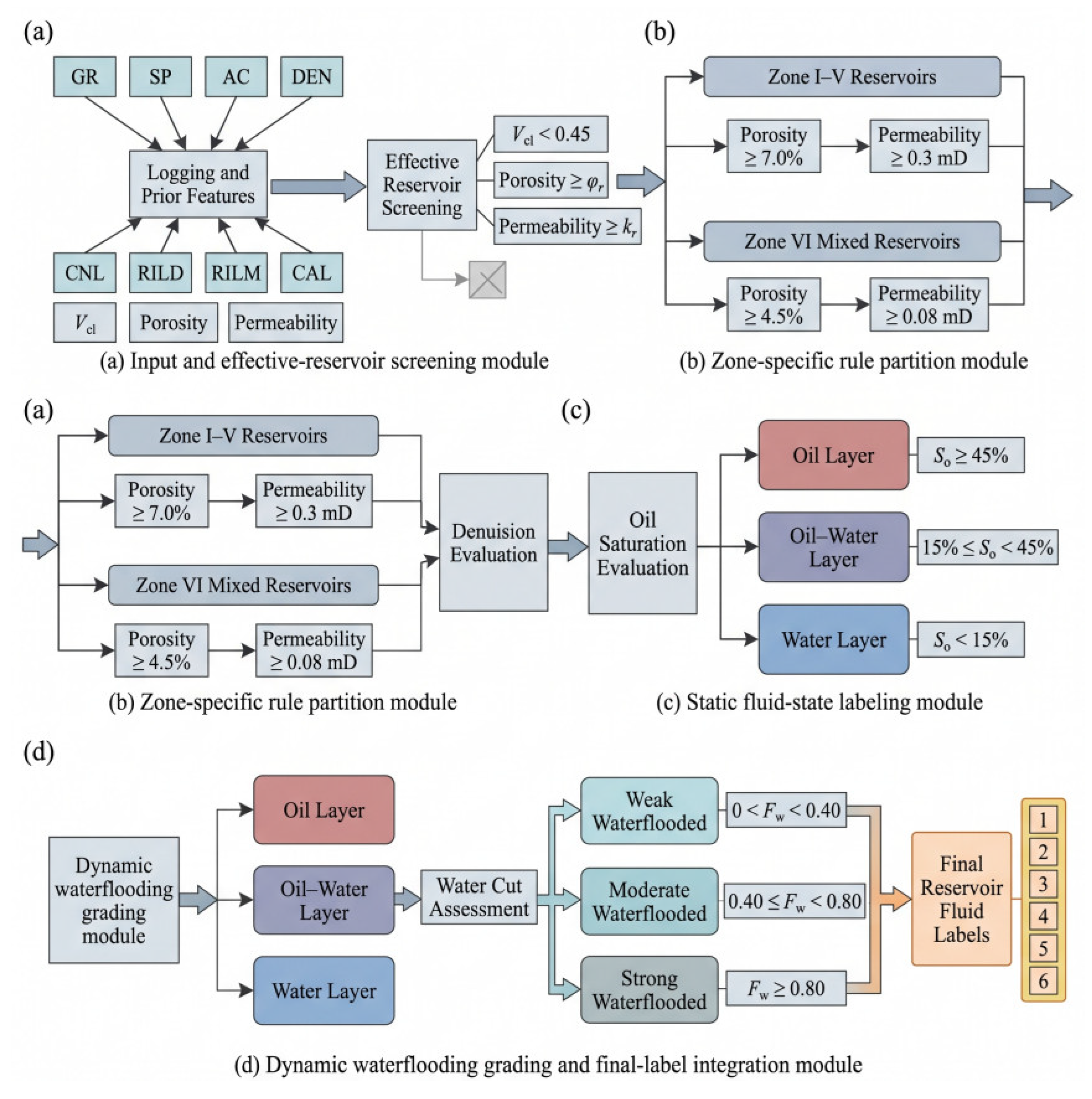
where $S_{o,i}$ denotes the oil saturation of the $i$-th sample. Reservoir-fluid identification criteria in the study area indicate that, under the condition of an effective reservoir, oil saturation can serve as an important discriminator among oil layers, oil–water layers, and water layers. Specifically, an oil saturation of 45% and higher corresponds to an oil layer; an oil saturation between 15% and 45% corresponds to an oil–water layer; and an oil saturation lower than 15% corresponds to a water layer. Meanwhile, the lower bounds for effective reservoirs are not identical across different stratigraphic units. For Type 1–5 intervals, the interpretation criteria generally require shale volume < 45%, porosity ≥ 7.0%, and permeability ≥ 0.3 mD, whereas Type 6 mixed-deposition intervals usually adopt the criteria of shale volume < 45%, porosity ≥ 4.5%, and permeability ≥ 0.08 mD.

To jointly account for static fluid identification and dynamic water-cut characteristics during the development stage, the reservoir-fluid label is uniformly constructed here as a joint categorical variable $y_i$. On the basis of oil layers, water layers, and oil–water layers, three additional states are introduced: weakly water-flooded, moderately water-flooded, and strongly water-flooded.

$$y_i=\left\{\begin{array}{ll}1,& V_{\mathrm{c}\mathrm{l},i}<0.45,\hspace{0.25em}{\varphi }_{e,i}\ge {\varphi }_r,\hspace{0.25em}{k}_i^{\mathrm{p}\mathrm{r}\mathrm{i}\mathrm{o}\mathrm{r}}\ge k_r,\hspace{0.25em}{S}_{o,i}\ge 0.45,\hspace{0.25em}{F}_{w,i}=0\\ 2,& V_{\mathrm{c}\mathrm{l},i}<0.45,\hspace{0.25em}{\varphi }_{e,i}\ge {\varphi }_r,\hspace{0.25em}{k}_i^{\mathrm{p}\mathrm{r}\mathrm{i}\mathrm{o}\mathrm{r}}\ge k_r,\hspace{0.25em}0.15\le S_{o,i}<0.45,\hspace{0.25em}{F}_{w,i}=0\\ 3,& V_{\mathrm{c}\mathrm{l},i}<0.45,\hspace{0.25em}{\varphi }_{e,i}\ge {\varphi }_r,\hspace{0.25em}{k}_i^{\mathrm{p}\mathrm{r}\mathrm{i}\mathrm{o}\mathrm{r}}\ge k_r,\hspace{0.25em}{S}_{o,i}<0.15,\hspace{0.25em}{F}_{w,i}=0\\ 4,& V_{\mathrm{c}\mathrm{l},i}<0.45,\hspace{0.25em}{\varphi }_{e,i}\ge {\varphi }_r,\hspace{0.25em}{k}_i^{\mathrm{p}\mathrm{r}\mathrm{i}\mathrm{o}\mathrm{r}}\ge k_r,\hspace{0.25em}0<F_{w,i}<0.40\\ 5,& V_{\mathrm{c}\mathrm{l},i}<0.45,\hspace{0.25em}{\varphi }_{e,i}\ge {\varphi }_r,\hspace{0.25em}{k}_i^{\mathrm{p}\mathrm{r}\mathrm{i}\mathrm{o}\mathrm{r}}\ge k_r,\hspace{0.25em}0.40\le F_{w,i}<0.80\\ 6,& V_{\mathrm{c}\mathrm{l},i}<0.45,\hspace{0.25em}{\varphi }_{e,i}\ge {\varphi }_r,\hspace{0.25em}{k}_i^{\mathrm{p}\mathrm{r}\mathrm{i}\mathrm{o}\mathrm{r}}\ge k_r,\hspace{0.25em}{F}_{w,i}\ge 0.80\end{array}\right.$$

(9)

where $y_i$ is the reservoir-fluid class label, $F_{w,i}$ is an auxiliary indicator representing the produced-fluid water cut, and ${\varphi }_r$ and $k_r$ denote the lower bounds of porosity and permeability associated with the corresponding stratigraphic-unit category, respectively. When $y_i=1,2,3$, the sample represents an oil layer, an oil–water layer, and a water layer, respectively; when $y_i=4,5,6$, it represents weak, moderate, and strong water flooding, respectively. Produced-fluid profile interpretation shows that weakly water-flooded intervals generally correspond to low to moderate water cut, moderately water-flooded intervals to moderate to relatively high water cut, and strongly water-flooded intervals to high water-cut production. Therefore, combining dynamic water-cut information with static saturation-based criteria helps improve the definition of water-flooding labels and enhances the discrimination of complex fluid states in the middle and late stages of reservoir development. It should be noted that water cut is only used as an auxiliary criterion for label construction rather than as an independent prediction target of YSF-Net. The model outputs are the six-class reservoir-fluid state and continuous water saturation. Thus, water cut mainly supports the definition of weakly, moderately, and strongly water-flooded intervals, while model evaluation focuses on fluid-state classification and S_w prediction.

Figure 2 illustrates the construction process of reservoir-fluid labels and the rule-based zonation criteria. The workflow includes effective-reservoir screening, zonation-based petrophysical thresholding, static oil–water state partitioning, and dynamic water-flooding grading. This label-construction strategy ensures that the six reservoir-fluid classes are defined not only by statistical labels, but also by geological and engineering interpretation criteria.

Figure 2. Construction of reservoir-fluid labels and rule-based zoning diagram.

2.3. Joint Prediction Framework and Optimization Objective Based on YSF-Net

After completing well-log sequence representation, reservoir-prior construction, and reservoir-fluid label definition, this study establishes a joint prediction framework based on YSF-Net, in which a shared feature encoder simultaneously outputs reservoir-fluid identification results and water-saturation predictions. Specifically, the network takes the input tensor obtained from Equation (3) as input, first extracts the morphological characteristics of the logging curves and the textures of adjacent intervals through local convolutional units, then captures long-range dependencies along the depth direction through a sequence-modeling module, and finally forms a shared representation for the central sample. Based on this shared representation, the classification branch and regression branch can be uniformly expressed as

$${\mathbf{h}}_i=f_{\mathrm{e}\mathrm{n}\mathrm{c}}\left({\mathbf{X}}_i;{\theta }_e\right),{\widehat{\mathbf{p}}}_i=\mathrm{S}\mathrm{o}\mathrm{f}\mathrm{t}\mathrm{m}\mathrm{a}\mathrm{x}\left({\mathbf{W}}_c{\mathbf{h}}_i+{\mathbf{b}}_c\right),{\widehat{S}}_{w,i}=\sigma \left({\mathbf{W}}_r{\mathbf{h}}_i+{\mathbf{b}}_r\right)$$

(10)

where ${\mathbf{X}}_i$ is the iii-th input sample, ${\mathbf{h}}_i$ is the shared feature representation, ${\widehat{\mathbf{p}}}_i$ is the probability distribution that the sample belongs to one of the six reservoir-fluid classes, and ${\widehat{S}}_{w,i}$ is the predicted water saturation. Here, $\sigma \left(\cdot \right)$ denotes the Sigmoid function, which constrains the output to the physically reasonable interval of [0, 1].

To ensure consistency among the classification results, saturation predictions, and regional geological–physical laws, the optimization objective in this study consists of a classification loss, a regression loss, and a physical consistency constraint. Specifically, the classification branch adopts the cross-entropy loss:

$${\mathcal{L}}_{\mathrm{c}\mathrm{l}\mathrm{s}}=-{\displaystyle \frac{1}{N}}{\displaystyle \sum _{i=1}^N}{\displaystyle \sum _{c=1}^C}{y}_{i,c}\mathrm{l}\mathrm{o}\mathrm{g}{\widehat{p}}_{i,c}$$

(11)

where $N$ is the number of training samples, $C=6$ is the number of classes, and $y_{i,c}$ is the ground-truth class indicator of the sample.

The regression branch adopts the Huber loss to improve the robustness of water-saturation prediction against anomalous samples:

$${\mathcal{L}}_{\mathrm{r}\mathrm{e}\mathrm{g}}={\displaystyle \frac{1}{N}}{\displaystyle \sum _{i=1}^N}\mathrm{H}\mathrm{u}\mathrm{b}\mathrm{e}\mathrm{r}\left({\widehat{S}}_{w,i}-S_{w,i}\right)$$

(12)

where $S_{w,i}$ is the true water saturation. Compared with the conventional mean squared error, the Huber loss maintains smooth optimization behavior when the error is small, while reducing the interference of large-error samples during training.

Furthermore, to ensure that the prediction results satisfy the regional electrical mechanism of the reservoir, a physical consistency constraint is constructed based on the modified Simandoux relationship in Equation (7) and is jointly optimized together with the classification and regression losses:

$$\mathcal{L}={\lambda }_1{\mathcal{L}}_{\mathrm{c}\mathrm{l}\mathrm{s}}+{\lambda }_2{\mathcal{L}}_{\mathrm{r}\mathrm{e}\mathrm{g}}+{\lambda }_3{\displaystyle \frac{1}{N}}{\displaystyle \sum _{i=1}^N}{\left[{\displaystyle \frac{1}{R_{t,i}}}-\left({\displaystyle \frac{V_{sh,i}}{R_{sh,g_i}}}+{\displaystyle \frac{{\varphi }_i^{m_{g_i}}}{a_{g_i}{R}_{w,g_i}{\widehat{S}}_{w,i}^{\hspace{0.17em}{n}_{g_i}}}}\right)\right]}^2$$

(13)

where ${\lambda }_1$, ${\lambda }_2$, and ${\lambda }_3$ are the weighting coefficients for the classification term, regression term, and physical-constraint term, respectively; $R_{t,i}$ is the true resistivity; $V_{sh,i}$ is the shale volume; ${\varphi }_i$ is the effective porosity; and $a_{g_i}$, $m_{g_i}$, $n_{g_i}$, $R_{w,g_i}$, and $R_{sh,g_i}$ are the electrical parameters, formation-water resistivity, and shale resistivity corresponding to the stratigraphic unit to which the sample belongs.

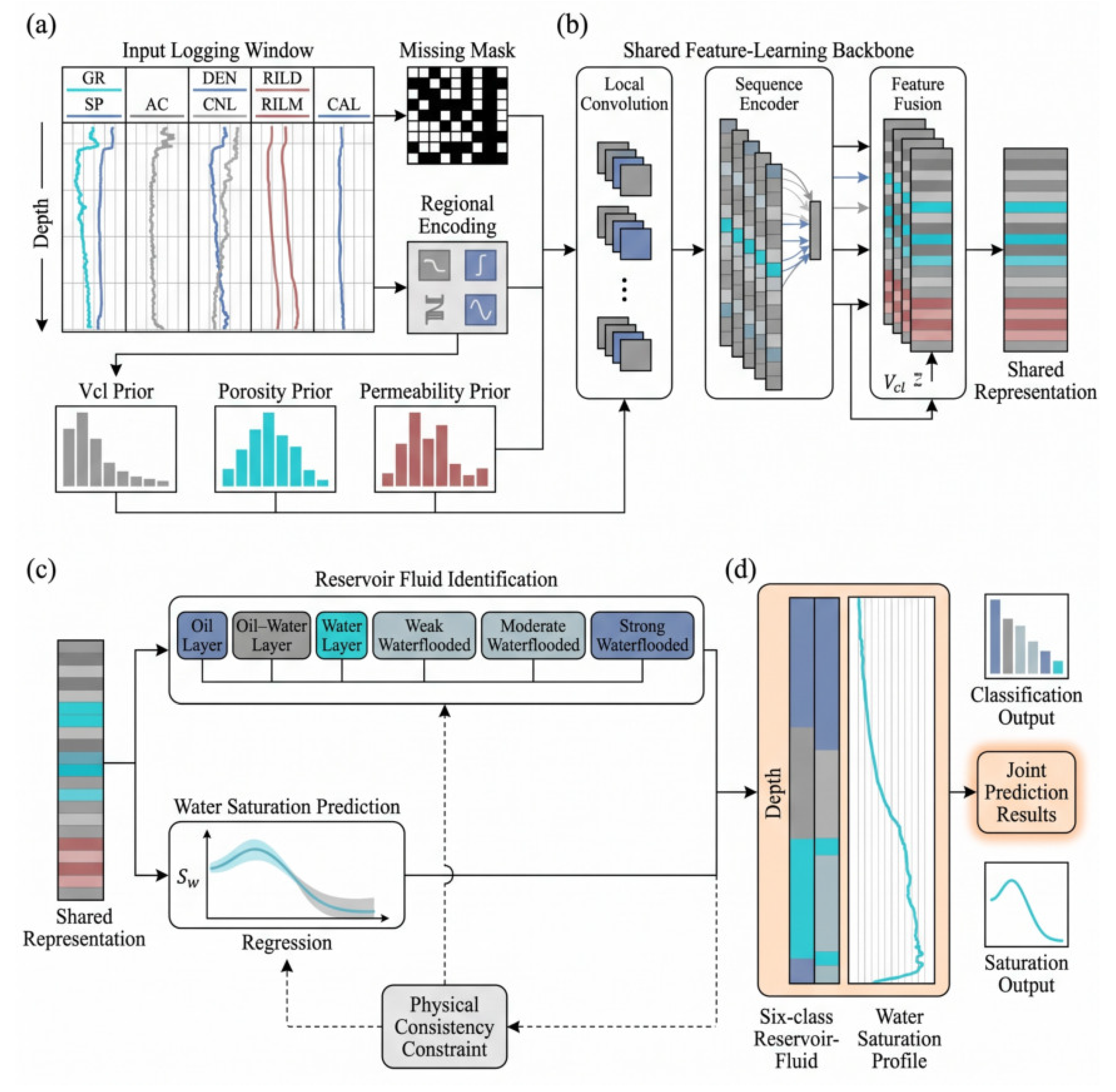
Figure 3 shows the overall joint prediction framework of YSF-Net. The model takes multi-log sequence windows, missing masks, regional embeddings, and reservoir-prior parameters as inputs. A shared feature encoder is used to extract local logging textures and vertical sequence dependencies, and two task-specific branches are then constructed for six-class reservoir-fluid identification and continuous water-saturation prediction. The classification and regression outputs are further constrained by physical consistency during model optimization.

Figure 3. Joint prediction framework of YSF-Net. (a) Input Feature and Geological Prior Construction: Multi-curve well-log data, missing masks, regional encoding, and geological priors are integrated to form the model input. (b) Shared Feature-Learning Backbone: Local convolution, sequence encoding, and feature fusion are used to extract a shared representation from the input logging features. (c) Joint Prediction Module: The shared representation is used for both reservoir fluid identification and water saturation prediction, with physical consistency constraints. (d) Joint Output Visualization: The final results include six-class reservoir fluid profiles, water saturation profiles, classification output, and saturation output.

In addition, a consistency constraint was introduced to align reservoir-fluid classes with continuous water-saturation values. This constraint ensures that oil layers correspond to relatively low S_w, whereas strongly water-flooded intervals correspond to high S_w, thereby reducing statistically possible but geologically unreasonable predictions. Through this joint optimization, YSF-Net integrates reservoir-fluid identification and water-saturation prediction within a unified feature space rather than treating them as independent tasks. This design is suitable for the fault-block reservoirs of the Youshashan Oilfield, where thin interbeds, strong architectural heterogeneity, and complex fluid transitions are common. The observed coupling among resistivity, acoustic transit time, density, shale content, and hydrocarbon-bearing properties also provides a geological basis for the physics-constrained joint learning strategy.

3. Data and Methods

3.1. Definition of Fluid Labels and Configuration of Comparative Methods

To ensure a fair comparison, four representative deep-learning baselines were selected: CNN, BiLSTM, CNN-BiLSTM, and Transformer. These models represent local-feature extraction, vertical sequence modeling, hybrid feature learning, and global dependency modeling, respectively. Therefore, they provide a systematic benchmark for evaluating the advantages of YSF-Net in intelligent well-log interpretation. Table 1 summarizes the sample composition of the six reservoir-fluid states. To avoid data leakage, 200 wells were split by well into 140 training wells, 30 validation wells, and 30 independent test wells. After depth resampling, outlier removal, effective-reservoir screening, and sliding-window construction, 420,000 valid samples were obtained. The six classes are relatively balanced, with oil layers, water layers, and strongly water-flooded layers accounting for 18.00%, 19.00%, and 20.00%, respectively, and oil–water layers, weakly water-flooded layers, and moderately water-flooded layers accounting for 14.00%, 15.00%, and 14.00%, respectively. Although severe class imbalance is absent, transition classes remain difficult to distinguish because of ambiguous oil–water contacts and water-flooding effects. Therefore, Macro-Precision, Macro-Recall, Macro-F1, and Macro-AUC were used together with Accuracy for a more objective evaluation.

Table 1. Sample distribution of the six reservoir-fluid states.

Class	Training Wells	Validation Wells	Test Wells	Training Samples	Validation Samples	Test Samples	Total Samples	Proportion
Oil layer	140	30	30	52,920	11,340	11,340	75,600	18.00%
Oil–water layer	140	30	30	41,160	8820	8820	58,800	14.00%
Water layer	140	30	30	55,860	11,970	11,970	79,800	19.00%
Weakly water-flooded layer	140	30	30	44,100	9450	9450	63,000	15.00%
Moderately water-flooded layer	140	30	30	41,160	8820	8820	58,800	14.00%
Strongly water-flooded layer	140	30	30	58,800	12,600	12,600	84,000	20.00%
Total	140	30	30	294,000	63,000	63,000	420,000	100.00%

To justify the input-feature selection, correlation analysis and SHAP-based feature-importance analysis were conducted between input features and reservoir-fluid labels. For correlation analysis, the six fluid states were encoded according to the transition order from oil-bearing to water-flooded intervals, and the absolute Spearman correlation coefficient was calculated for each feature. For SHAP analysis, validation-well samples were used to interpret the trained YSF-Net model, and the mean absolute SHAP value was adopted to quantify each feature’s contribution to classification. The results are summarized in Table 2.

Table 2. Feature screening results based on correlation and SHAP analysis.

Feature	Geological Meaning	Absolute Spearman Correlation	Mean Absolute SHAP Value	Selection Result
RILD	Deep resistivity response	0.42	0.156	Retained
RILM	Medium/shallow resistivity response	0.39	0.141	Retained
Vcl	Shale-volume prior	0.35	0.124	Retained
Porosity	Reservoir pore-space prior	0.31	0.109	Retained
Permeability	Flow-capacity prior	0.28	0.094	Retained
SP	Sand–mud and permeability-related response	0.25	0.083	Retained
CNL	Neutron porosity response	0.23	0.076	Retained
DEN	Density and pore-structure response	0.21	0.068	Retained
AC	Acoustic and compaction response	0.18	0.059	Retained
GR	Shale-content response	0.17	0.054	Retained
CAL	Borehole condition indicator	0.08	0.026	Auxiliary feature

3.2. Evaluation Metrics and Experimental Protocol Design

To comprehensively evaluate the proposed model, Accuracy, Macro-Precision, Macro-Recall, Macro-F1, and Macro-AUC were used for six-class reservoir-fluid identification, while S_w RMSE, MAE, and R² were used for water-saturation prediction. Parameter size and per-sample inference time were also reported to assess deployment efficiency.

To verify cross-well generalization and avoid data leakage, a strict well-based splitting strategy was adopted. The 200 wells were divided into 140 training wells, 30 validation wells, and 30 independent test wells, with no overlap among subsets. All subsets covered delta-front clastic reservoirs, distal front transitional reservoirs, and mixed-deposition reservoirs. Specifically, Type 1–3 intervals mainly correspond to delta-front clastic reservoirs, Type 4–5 intervals to distal front transitional reservoirs, and Type 6 intervals to mixed-deposition reservoirs. During testing, model parameters, normalization statistics, and discrimination thresholds were fixed, and no test-well labels were used for retraining, fine-tuning, or threshold calibration. Thus, the reported results reflect the direct transfer performance on unseen wells under different stratigraphic and depositional backgrounds.

A well-based five-fold cross-validation experiment was further conducted to evaluate robustness. The 200 wells were divided into five non-overlapping groups, and the model was retrained from scratch in each fold. The average results were Accuracy = 0.923 ± 0.004, Macro-F1 = 0.910 ± 0.005, and S_w RMSE = 0.063 ± 0.002, indicating stable generalization under different well partitions. Hyperparameters were determined using a two-stage strategy combining coarse grid search and Bayesian optimization. Window length, hidden dimension, attention heads, dropout, learning rate, batch size, and weight decay were only tuned on the validation wells. The final settings were window length = 33, hidden dimension = 64, attention heads = 4, dropout = 0.10, learning rate = 3 × 10⁻⁴, batch size = 256, weight decay = 1 × 10⁻⁴, and AdamW optimizer. The loss weights were selected according to validation performance. Since reservoir-fluid classification was the primary task, λ₁ was fixed at 1.0, while λ₂ and λ₃ were tuned to balance S_w regression and physical consistency. The final values were λ₁ = 1.0, λ₂ = 0.8, and λ₃ = 0.2. For ablation experiments, a single-variable control strategy was used: only one module was removed at a time, while the data split, preprocessing, optimizer, learning rate, batch size, random seed, and early stopping strategy remained unchanged. Therefore, the performance differences can be attributed to the corresponding modules rather than changes in training conditions.

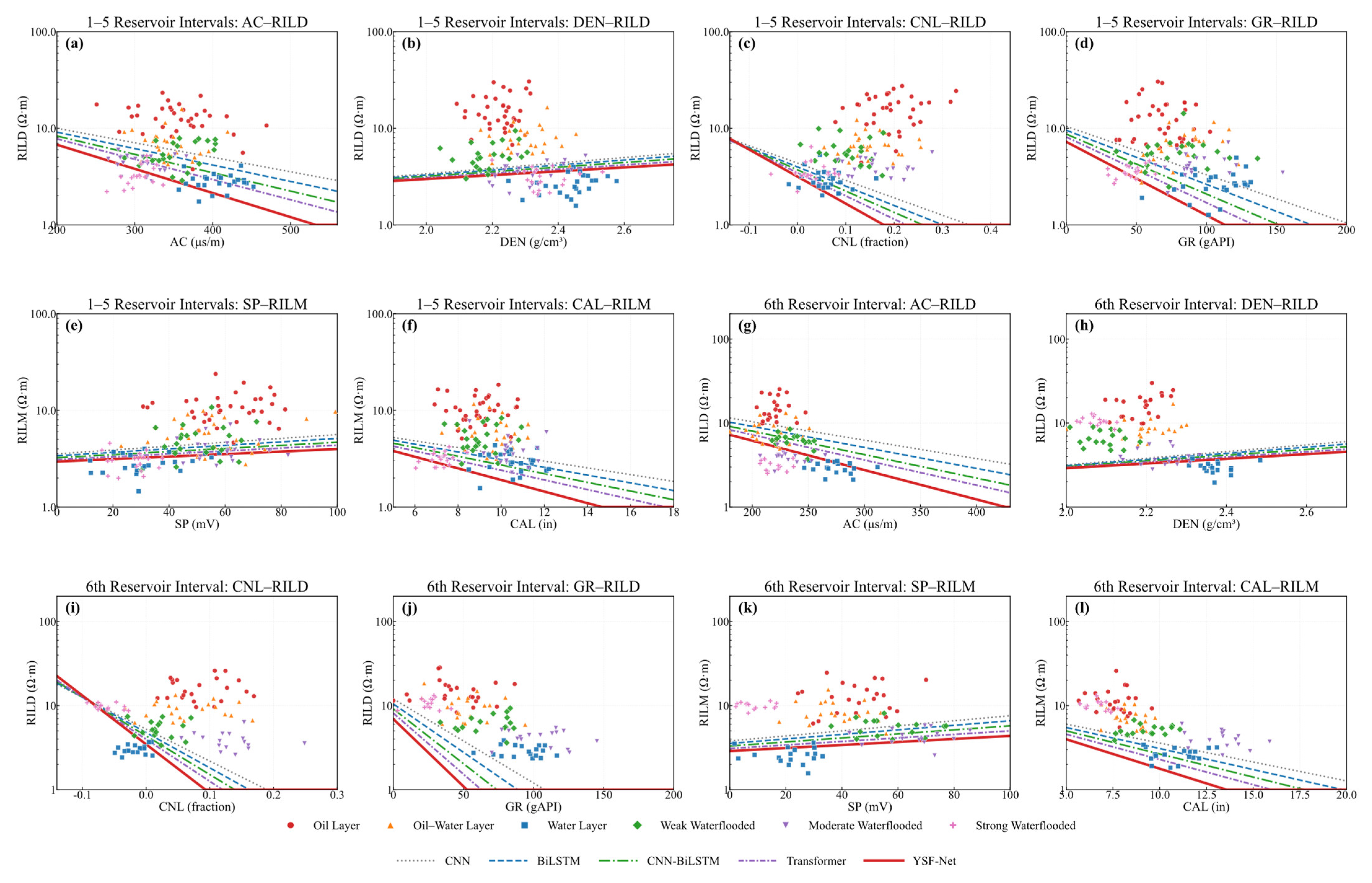
Figure 4 shows typical well-log cross-plots and fitting boundaries under different reservoir zonations. Type 1–5 intervals and Type 6 mixed-deposition reservoirs exhibit distinct relationships in AC–RILD, DEN–RILD, CNL–RILD, GR–RILD, SP–RILM, and CAL–RILM cross-plots, especially in class aggregation patterns and empirical boundary trends, indicating that fluid-identification mechanisms vary among reservoir types. Therefore, regional stratigraphic constraints and prior parameters are introduced into the network input, allowing geological zonation information to participate in feature learning and reducing confusion between oil-bearing and water-bearing classes caused by a unified discrimination boundary.

Figure 4. Logging crossplots and empirical boundary charts for different reservoir zones. (a) 1–5 Reservoir Intervals: AC–RILD: Shows the relationship between acoustic logging and deep resistivity for the first to fifth reservoir intervals. (b) 1–5 Reservoir Intervals: DEN–RILD: Shows the density–resistivity response characteristics of the first to fifth reservoir intervals. (c) 1–5 Reservoir Intervals: CNL–RILD: Shows the neutron porosity and deep resistivity distribution for the first to fifth reservoir intervals. (d) 1–5 Reservoir Intervals: GR–RILD: Shows the relationship between gamma ray and deep resistivity for the first to fifth reservoir intervals. (e) 1–5 Reservoir Intervals: SP–RILM: Shows the spontaneous potential and medium resistivity response for the first to fifth reservoir intervals. (f) 1–5 Reservoir Intervals: CAL–RILM: Shows the borehole diameter and medium resistivity response for the first to fifth reservoir intervals. (g) 6th Reservoir Interval: AC–RILD: Shows the acoustic logging and deep resistivity relationship in the sixth reservoir interval. (h) 6th Reservoir Interval: DEN–RILD: Shows the density and deep resistivity response characteristics of the sixth reservoir interval. (i) 6th Reservoir Interval: CNL–RILD: Shows the neutron porosity and deep resistivity distribution in the sixth reservoir interval. (j) 6th Reservoir Interval: GR–RILD: Shows the gamma ray and deep resistivity relationship in the sixth reservoir interval. (k) 6th Reservoir Interval: SP–RILM: Shows the spontaneous potential and medium resistivity response in the sixth reservoir interval. (l) 6th Reservoir Interval: CAL–RILM: Shows the borehole diameter and medium resistivity response in the sixth reservoir interval.

4. Results and Discussion

4.1. Comparative Analysis of the Overall Performance of Different Methods

Table 3 presents the overall performance of different methods for six-class reservoir-fluid identification and water-saturation prediction. Overall, the model performance improves progressively with enhanced feature-learning capability. CNN achieves an Accuracy of 0.883, a Macro-F1 of 0.867, and an S_w RMSE of 0.086. After introducing vertical sequence modeling, BiLSTM improves the Accuracy to 0.894 and reduces the S_w RMSE to 0.078. CNN-BiLSTM further integrates local and sequential features, increasing the Accuracy to 0.907 and the Macro-AUC to 0.951. The Transformer, benefiting from global dependency modeling, further improves both the classification and regression performance, with an Accuracy of 0.913 and an S_w R² of 0.931.

Table 3. Overall performance comparison of different methods.

Method	Accuracy	Macro-Precision	Macro-Recall	Macro-F1	Macro-AUC	Sw RMSE	Sw MAE	Sw R2
CNN	0.883	0.871	0.864	0.867	0.931	0.086	0.067	0.892
BiLSTM	0.894	0.883	0.876	0.879	0.941	0.078	0.061	0.907
CNN-BiLSTM	0.907	0.897	0.891	0.894	0.951	0.071	0.055	0.923
Transformer	0.913	0.904	0.899	0.901	0.958	0.068	0.052	0.931
YSF-Net	0.926	0.918	0.909	0.913	0.968	0.061	0.047	0.947

YSF-Net achieves the best results across all metrics, with an Accuracy of 0.926, a Macro-F1 of 0.913, and a Macro-AUC of 0.968. Its S_w RMSE and MAE decrease to 0.061 and 0.047, respectively, while S_w R² increases to 0.947. Compared with the Transformer, YSF-Net improves the Accuracy and Macro-F1 by 1.3 and 1.2 percentage points, respectively, and reduces the S_w RMSE by 0.007. Compared with CNN-BiLSTM, it improves both the Accuracy and Macro-F1 by 1.9 percentage points and reduces S_w RMSE by 0.010. These results demonstrate that the integration of regional constraints, reservoir-prior inputs, multi-task learning, and physical consistency effectively enhances both reservoir-fluid identification and water-saturation prediction.

To further clarify the academic marginal contribution of YSF-Net, representative recent studies on reservoir-fluid identification and water-saturation prediction were compared, as shown in Table 4. Because these studies used different datasets and task settings, the comparison is mainly used to summarize methodological differences and reported performances.

Table 4. Quantitative comparison with representative recent studies.

Method/Study	Main Task	Reported Result	Similarity/Difference from YSF-Net
Guo et al. [11]	Saturation determination and fluid identification	Fluid identification Accuracy of about 89.55–89.95%	Similarity: Both focus on fluid identification and saturation-related interpretation. Difference: Mainly based on petrophysical formulas and empirical rules without deep joint prediction of six-class fluid states and Sw.
Hua et al. [15]	Reservoir-fluid identification	Overall prediction Accuracy higher than 94%	Similarity: Both use intelligent models for reservoir-fluid identification. Difference: Mainly focuses on fluid classification and does not jointly predict continuous Sw.
Li et al. [20]	Reservoir-fluid identification	Average Accuracy of 91.41%	Similarity: Both aim to improve reservoir-fluid classification. Difference: Uses a traditional machine-learning classifier and lacks physical consistency constraints.
Gohari Nezhad and Emami Niri [10]	Water-saturation prediction	Blind-well R2 = 0.859; 10-fold average R2 = 0.968	Similarity: Both involve Sw prediction from well logs. Difference: Focuses on Sw regression only without reservoir-fluid state classification.
YSF-Net in this study	Six-class reservoir-fluid identification + Sw prediction	Accuracy = 0.926; Macro-F1 = 0.913; Sw RMSE = 0.061; Sw R2 = 0.947	Jointly performs six-class fluid identification and continuous Sw prediction with regional priors, multi-task learning, and physical consistency constraints.

As shown in Table 4, most recent studies focus on either reservoir-fluid identification or water-saturation prediction. In contrast, YSF-Net jointly performs six-class reservoir-fluid identification and continuous S_w prediction while incorporating regional priors and physical consistency constraints. This indicates that the proposed method provides a more integrated and geologically constrained solution for complex reservoir interpretation.

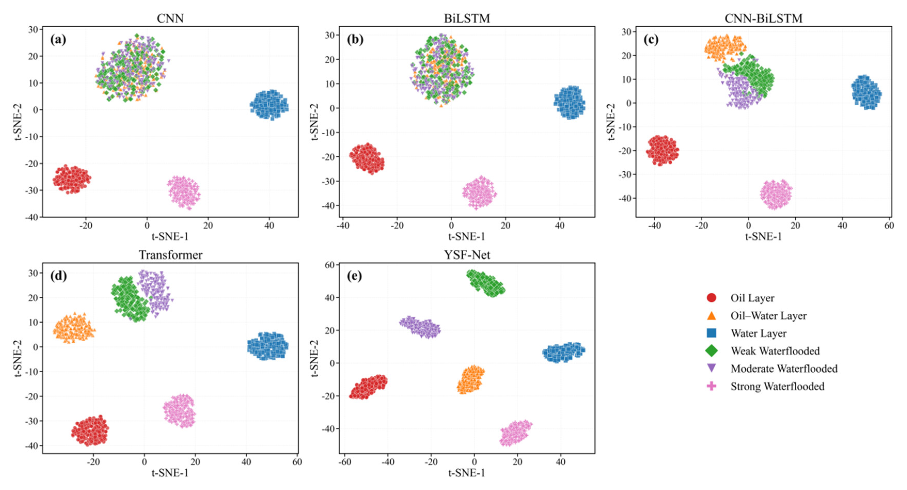
To further evaluate the feature-space separability of different methods, Figure 5 presents the t-SNE visualization results. CNN and BiLSTM can roughly distinguish oil layers, water layers, and strongly water-flooded layers, but obvious overlap remains among oil–water layers, weakly water-flooded layers, and moderately water-flooded layers. CNN-BiLSTM and the Transformer improve feature aggregation to some extent, yet category boundaries are still partially mixed. In contrast, the YSF-Net produces the most compact feature clusters and the clearest inter-class separation, especially for oil–water layers and intervals with different flooding intensities. This suggests that the YSF-Net learns a joint representation with stronger structural consistency and geological coherence rather than relying on shallow discrimination dominated by a single logging curve, thereby providing a more stable feature basis for both classification and regression tasks.

Figure 5. t-SNE visualization results of feature representations learned by different methods. (a) CNN: Shows the t-SNE feature distribution obtained by the CNN model, with partial overlap among different reservoir fluid classes. (b) BiLSTM: Shows the t-SNE feature distribution obtained by the BiLSTM model, where some classes are separated but several categories still overlap. (c) CNN-BiLSTM: Shows the t-SNE feature distribution obtained by the CNN-BiLSTM model, with improved class separation compared with single models. (d) Transformer: Shows the t-SNE feature distribution obtained by the Transformer model, where most reservoir fluid classes form clearer clusters. (e) YSF-Net: Shows the t-SNE feature distribution obtained by the proposed YSF-Net model, with the clearest class separation and more compact clusters.

4.2. Analysis of Recognition Performance for Individual Classes and Their Confusion Characteristics

Table 5 further presents the class-wise identification performance of YSF-Net for the six reservoir-fluid classes. Oil layers and strongly water-flooded layers show the best recognition results, with Precision, Recall, and F1-score all exceeding 0.944 and AUC values of 0.959 and 0.961, respectively. This indicates that these two classes have relatively stable and distinctive petrophysical and fluid-response characteristics.

Table 5. Comparison of classification performance for each category of YSF-Net.

Class	Precision	Recall	F1-Score	AUC
Oil layer	0.944	0.936	0.940	0.978
Oil–water layer	0.886	0.871	0.878	0.951
Water layer	0.927	0.913	0.920	0.969
Weakly water-flooded layer	0.902	0.886	0.894	0.960
Moderately water-flooded layer	0.891	0.874	0.882	0.955
Strongly water-flooded layer	0.959	0.964	0.961	0.985
Macro average	0.918	0.909	0.913	0.968

By contrast, oil–water layers, moderately water-flooded layers, and weakly water-flooded layers show a slightly lower performance, with F1-scores of 0.878, 0.882, and 0.894, respectively. This is consistent with practical interpretation, as transitional reservoir intervals often exhibit mixed oil- and water-layer logging responses, while different flooding intensities usually change gradually. Therefore, cross-class confusion is more likely to occur. Nevertheless, the AUC values of YSF-Net for these difficult classes remain around 0.95, indicating that the model still has a strong discrimination ability for categories with ambiguous boundaries.

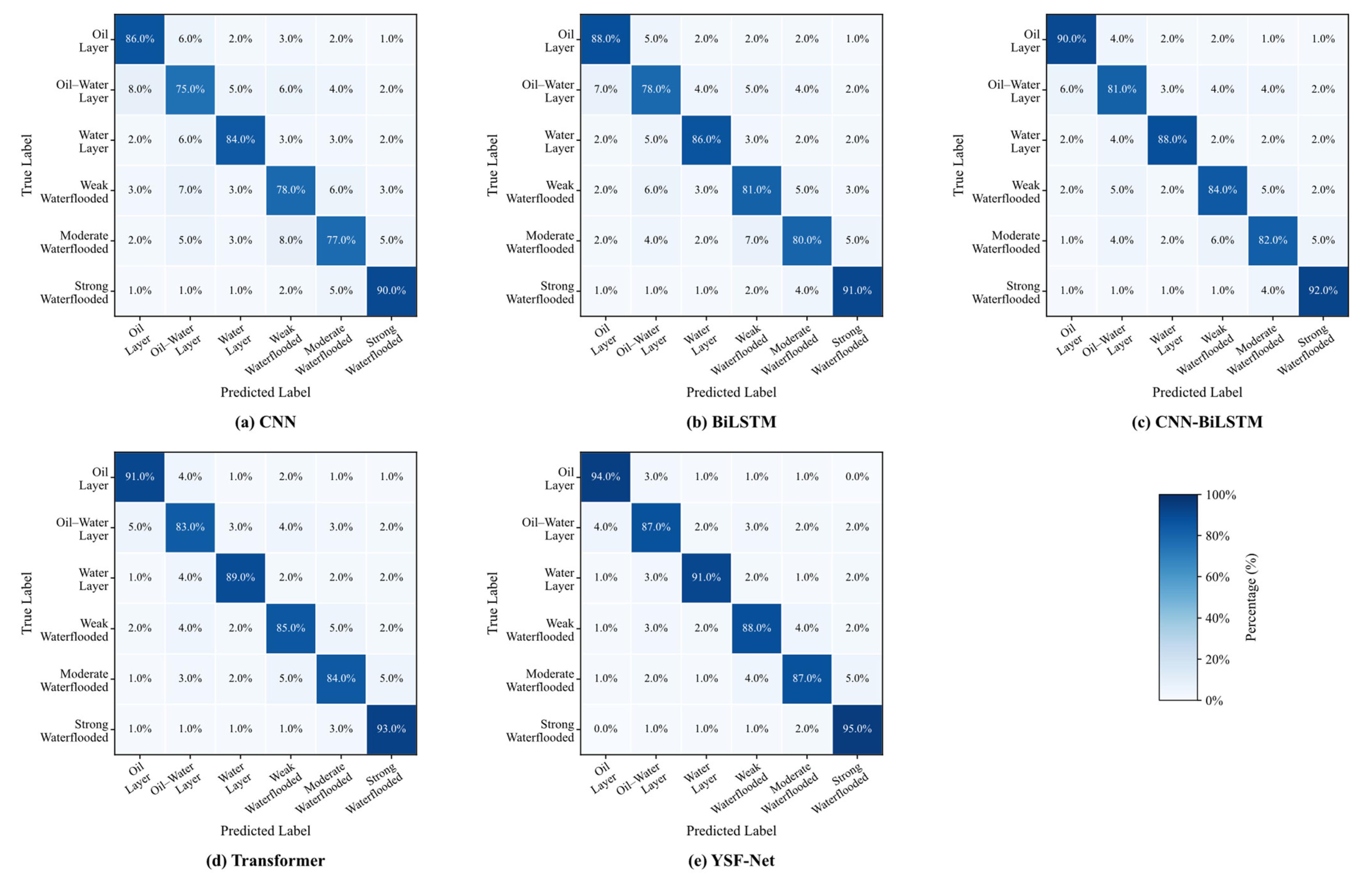
Figure 6 shows the confusion matrices of different methods. From CNN to YSF-Net, the diagonal dominance becomes stronger and off-diagonal errors decrease, indicating an improved classification performance. CNN shows obvious confusion between oil–water layers and weakly water-flooded layers, as well as between weakly and moderately water-flooded layers. BiLSTM and CNN-BiLSTM reduce these errors, but adjacent-class confusion remains. The Transformer performs better overall, yet still shows confusion between moderately and strongly water-flooded layers and between oil–water layers and water layers. The YSF-Net achieves the clearest diagonal dominance, with more stable recognition of oil layers, water layers, and strongly water-flooded layers, while reducing errors in transitional categories. This suggests that the YSF-Net improves both the overall Accuracy and class-boundary discrimination, producing predictions more consistent with the gradual transition from oil-bearing to water-bearing reservoirs.

Figure 6. Comparison of six-class confusion matrices for different methods.

To further examine the ambiguous boundary between oil–water layers and water-flooded layers, transition-boundary samples were statistically analyzed using 200 wells and 420,000 valid samples, as shown in Table 6. Samples located between adjacent classes, near oil–water saturation thresholds, or with small probability margins between the top two predicted classes were defined as transition-boundary samples. In total, 48,200 such samples were identified, accounting for 11.48% of the dataset. Among them, the oil–water layer–weakly water-flooded layer boundary had the largest proportion, with 13,462 samples and the lowest mean probability margin of 0.186, indicating strong feature overlap and poor separability. This is consistent with practical interpretation, as both classes may show moderate resistivity, increased water saturation, weakened deep–shallow resistivity contrast, and similar porosity–permeability conditions. The weakly–moderately and moderately–strongly water-flooded boundaries also account for considerable proportions, confirming that water-flooding intensity changes gradually rather than abruptly. For these ambiguous boundaries, the YSF-Net achieves accuracies of 0.862, 0.881, and 0.889, respectively, demonstrating a stable discrimination capability. This improvement mainly benefits from the joint use of multiple logs, reservoir-prior parameters, and multi-task optimization, which uses continuous water-saturation prediction to constrain fluid-state boundaries and reduce unreasonable jumps in transition zones.

Table 6. Discrimination statistics of typical transition-boundary samples.

Transition-Boundary Type	Number of Transition Samples	Proportion of Transition Samples	Proportion of Total Samples	Main Discrimination Basis	Mean Probability Margin	Boundary-Sample Accuracy of YSF-Net
Oil–water layer vs. weakly water-flooded layer	13,462	27.93%	3.20%	Moderate resistivity, increased water saturation, weakened deep–shallow resistivity contrast	0.186	0.862
Weakly vs. moderately water-flooded layer	12,080	25.06%	2.88%	Increased water saturation, enhanced production water-flooding intensity, changes in porosity–permeability conditions	0.203	0.881
Moderately vs. strongly water-flooded layer	11,640	24.15%	2.77%	High water saturation, low resistivity response, enhanced water-flooding intensity	0.215	0.889
Oil–water layer vs. water layer	7160	14.85%	1.70%	Decreased oil saturation, increased water saturation, electrical response migrating toward water-layer characteristics	0.226	0.894
Other adjacent boundaries	3858	8.00%	0.92%	Local thin beds, reservoir heterogeneity, and logging-response disturbance	0.238	0.904
Total	48,200	100.00%	11.48%	—	0.207	0.882

Misclassified samples were analyzed in terms of geological position, logging response, saturation interval, and prediction confidence. Most errors occur in transition intervals rather than stable oil or water layers. These errors are mainly caused by overlapping responses between oil–water layers and weakly water-flooded layers, gradual boundaries between weakly and moderately water-flooded layers, reduced resistivity sensitivity in high water-cut intervals, and local disturbances from thin beds, borehole enlargement, or heterogeneous sand–mud interbeds.

These findings suggest that YSF-Net errors are concentrated in geologically reasonable transition zones rather than caused by random classification failure. Therefore, the model is more applicable to reservoirs with complete conventional logs, clear stratigraphic zonation, and available reservoir-prior parameters. For reservoirs significantly different from the training area, such as carbonate, coal-bearing, or gas-bearing reservoirs, as well as intervals with long continuous missing curves, local recalibration or fine-tuning is recommended. Thus, the YSF-Net should be used as a geology-assisted intelligent interpretation tool rather than a complete substitute for expert interpretation.

4.3. Analysis of Water-Saturation Prediction Performance and Error Characteristics

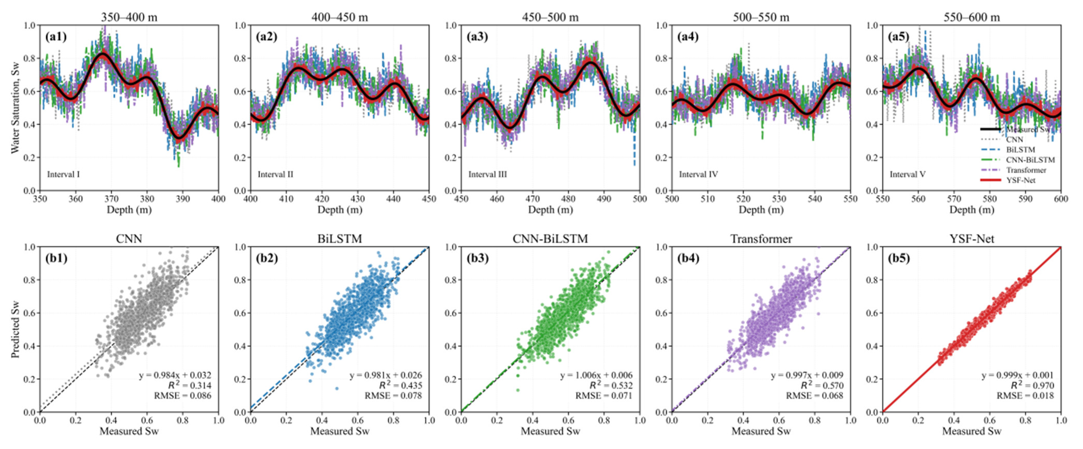
In addition to the classification results, Figure 7 shows the local well-interval water-saturation prediction curves and the scatter fitting relationships between measured and predicted values. The CNN and BiLSTM exhibit relatively coarse tracking of local fluctuations, with insufficient peak restoration or local noise amplification. The CNN-BiLSTM and Transformer better capture the overall trend but still show deviations at abrupt-change points and transition intervals. In contrast, the YSF-Net achieves the closest agreement with measured water saturation in fluctuation trend, peak position, and local turning points, with scatter points more concentrated around the 1:1 reference line. This indicates that the YSF-Net not only reduces the overall regression error, but also better preserves the continuous variation characteristics of water saturation within local intervals.

Figure 7. Comparison of local water saturation prediction and scatter fitting results for different methods. (a1) Interval I: Shows the measured and predicted water saturation profiles in the depth interval of 350–400 m. (a2) Interval II: Shows the comparison between measured and predicted water saturation in the 400–450 m interval. (a3) Interval III: Shows the water saturation prediction results in the 450–500 m interval. (a4) Interval IV: Shows the matching degree between measured and predicted water saturation in the 500–550 m interval. (a5) Interval V: Shows the water saturation prediction performance in the 550–600 m interval. (b1) CNN: Shows the fitting relationship between measured and predicted water saturation using the CNN model. (b2) BiLSTM: Shows the water saturation fitting result obtained by the BiLSTM model. (b3) CNN-BiLSTM: Shows the measured–predicted water saturation fitting result of the CNN-BiLSTM model. (b4) Transformer: Shows the water saturation prediction fitting performance of the Transformer model. (b5) YSF-Net: Shows the fitting result of the proposed YSF-Net model, with the closest agreement between measured and predicted water saturation.

Table 7 presents the ablation results of the YSF-Net. The complete model outperforms all ablated variants in Accuracy, Macro-F1, Macro-AUC, and S_w prediction metrics, confirming the necessity of each component. Removing the regional zonation constraint reduces the Accuracy to 0.907 and Macro-F1 to 0.895, indicating that geological zonation helps constrain class boundaries. Removing the physical constraint causes a limited decline in classification performance but increases the S_w RMSE to 0.074 and decreases S_w R² to 0.919, suggesting that physical consistency mainly improves water-saturation prediction. When multi-task learning is removed, both classification and S_w prediction performance deteriorate, confirming the complementarity between fluid-state identification and water-saturation regression. The largest performance drop occurs after removing prior-parameter inputs, with Accuracy decreasing to 0.898 and Macro-F1 to 0.885, indicating that parameters such as Vcl, porosity, and permeability effectively enhance reservoir-quality and fluid-difference characterization. Overall, the improvement of the YSF-Net results from the coordinated contribution of multiple components rather than a single module.

Table 7. Ablation experiment results of YSF-Net.

Model	Accuracy	Macro-F1	Macro-AUC	Sw RMSE	Sw MAE	Sw R2
Without regional zonation constraint	0.907	0.895	0.953	0.071	0.055	0.926
Without physical constraint term	0.911	0.899	0.956	0.074	0.057	0.919
Without multi-task joint learning	0.903	0.891	0.949	0.076	0.059	0.914
Without prior-parameter input (Vcl, POR, K)	0.898	0.885	0.946	0.079	0.061	0.908
Complete YSF-Net	0.926	0.913	0.968	0.061	0.047	0.947

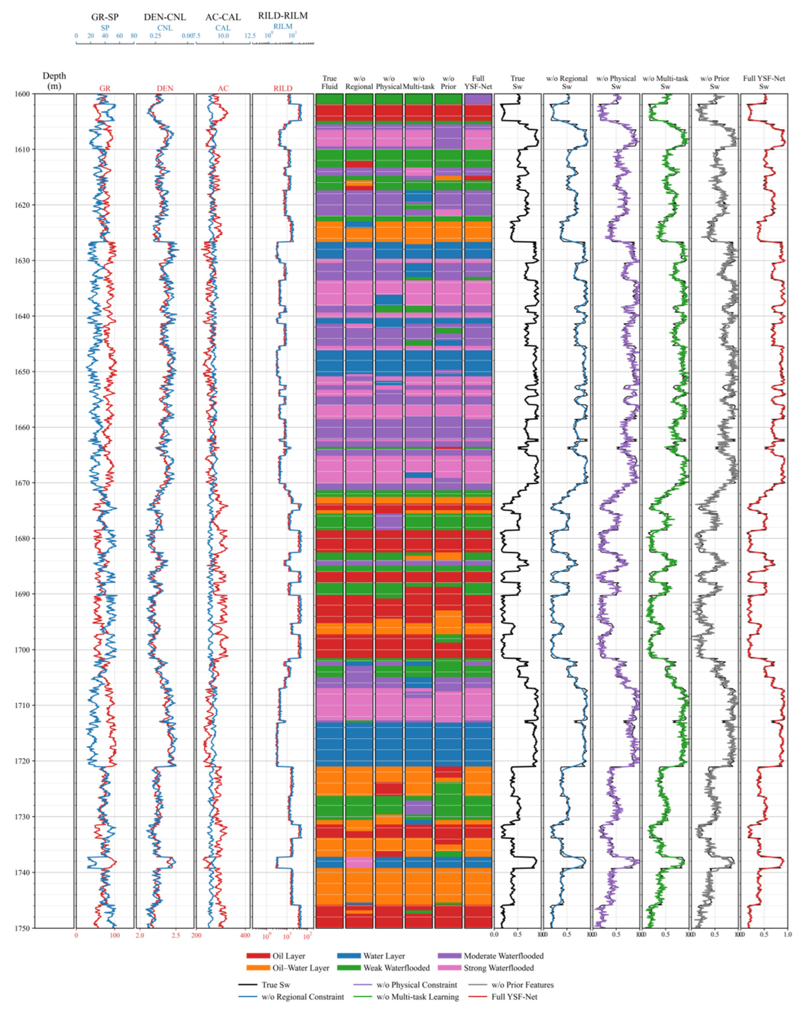
Figure 8 further shows the output variations in different ablated models in typical well intervals. Without the regional zonation constraint, the model is more prone to banded misclassification near local boundaries and adjacent class-transition zones, indicating that regional information helps stabilize the discrimination of stratigraphic units and reservoir types. Removing the physical constraint preserves the overall trend of the predicted curve but increases local deviations in peak position and amplitude, suggesting that this module mainly improves the rationality of S_w prediction. Without multi-task learning, the consistency between fluid labels and water-saturation curves decreases, confirming the mutual benefit of classification and regression. Removing the prior-parameter input leads to more obvious instability in both fluid identification and S_w prediction, further highlighting the importance of reservoir-prior information. Overall, the complete YSF-Net performs best in fluid-band continuity, boundary correspondence, and water-saturation fitting, consistent with the quantitative results in Table 5. This demonstrates that the performance gain of the proposed method arises from the coordinated effects of regional zonation constraints, physical consistency, multi-task learning, and prior-parameter input rather than accidental data fitting.

Figure 8. Comparison of typical well intervals in the YSF-Net ablation experiments.

4.4. Analysis of Cross-Well Generalization Ability and Stratigraphic Adaptability

It should be noted that the cross-well results in Table 8 were obtained under a direct transfer setting, where the training, validation, and test wells were completely separated by well identity. The 30 independent test wells were not used for training, parameter updating, threshold calibration, or fine-tuning, and the fixed model was directly applied after training and validation. These test wells covered delta-front clastic reservoirs, distal front transitional reservoirs, and mixed-deposition reservoirs, enabling the evaluation of both unseen-well generalization and adaptability to different depositional backgrounds. As shown in Table 8, the YSF-Net achieves the highest Cross-well Accuracy and Cross-well Macro-F1 of 0.918 and 0.904, respectively, with the lowest Cross-well S_w RMSE of 0.064, indicating that it captures stable logging–fluid relationships rather than well-specific patterns. Table 8 further shows that the YSF-Net maintains the best cross-well performance while requiring only 2.08 M parameters and 0.86 ms/sample, outperforming the Transformer with lower model complexity and faster inference. Although not the lightest model, YSF-Net achieves a favorable balance between Accuracy, stability, and deployment efficiency, making it suitable for practical well-log interpretation.

Table 8. Comparison of cross-well generalization and efficiency of different methods.

Method	Cross-Well Accuracy	Cross-Well Macro-F1	Cross-Well Sw RMSE	Params (M)	Inference Time (ms/Sample)
CNN	0.869	0.852	0.091	0.82	0.41
BiLSTM	0.881	0.866	0.083	1.24	0.68
CNN-BiLSTM	0.896	0.883	0.075	1.73	0.79
Transformer	0.902	0.891	0.072	2.46	0.94
YSF-Net	0.918	0.904	0.064	2.08	0.86

The inference time was measured on a workstation equipped with an Intel Core i9-13900K CPU, 64 GB RAM, and an NVIDIA GeForce RTX 4090 GPU with 24 GB memory. The software environment included Python 3.10, PyTorch 2.1, and CUDA 12.1. The batch size during inference was set to 256. The inference time represents the average forward-propagation time per sample on the independent test-well samples, excluding data loading, preprocessing, and post-processing.

Table 9 presents the reservoir-type-specific results. The YSF-Net performs best in delta-front clastic reservoirs, corresponding to Type 1–3 intervals, with an Accuracy of 0.938, a Macro-F1 of 0.927, and an S_w RMSE of 0.055. In distal front transitional reservoirs, corresponding to Type 4–5 intervals, the metrics decrease slightly but remain at high levels. Mixed-deposition reservoirs, corresponding to Type 6 intervals, show the greatest prediction difficulty, with an Accuracy of 0.902, a Macro-F1 of 0.888, and an S_w RMSE of 0.071. This is mainly attributed to stronger lithologic mixing, less stable logging responses, and more pronounced internal heterogeneity. Overall, the YSF-Net maintains an Accuracy of approximately 0.90 or higher and a low S_w error across all reservoir types, indicating good adaptability to different sedimentary backgrounds.

Table 9. Comparison of identification and prediction performance on different reservoir types.

Reservoir Type	Accuracy	Macro-Precision	Macro-Recall	Macro-F1	Macro-AUC	Sw RMSE	Sw MAE	Sw R2
Delta-front clastic reservoir (Type 1–3 intervals)	0.938	0.931	0.924	0.927	0.974	0.055	0.042	0.956
Distal front transitional reservoir (Type 4–5 intervals)	0.921	0.913	0.904	0.908	0.965	0.063	0.048	0.944
Mixed-deposition reservoir (Type 6 intervals)	0.902	0.893	0.884	0.888	0.952	0.071	0.055	0.927
Overall	0.926	0.918	0.909	0.913	0.968	0.061	0.047	0.947

4.5. Validation of Joint Prediction Results in Typical Well Intervals

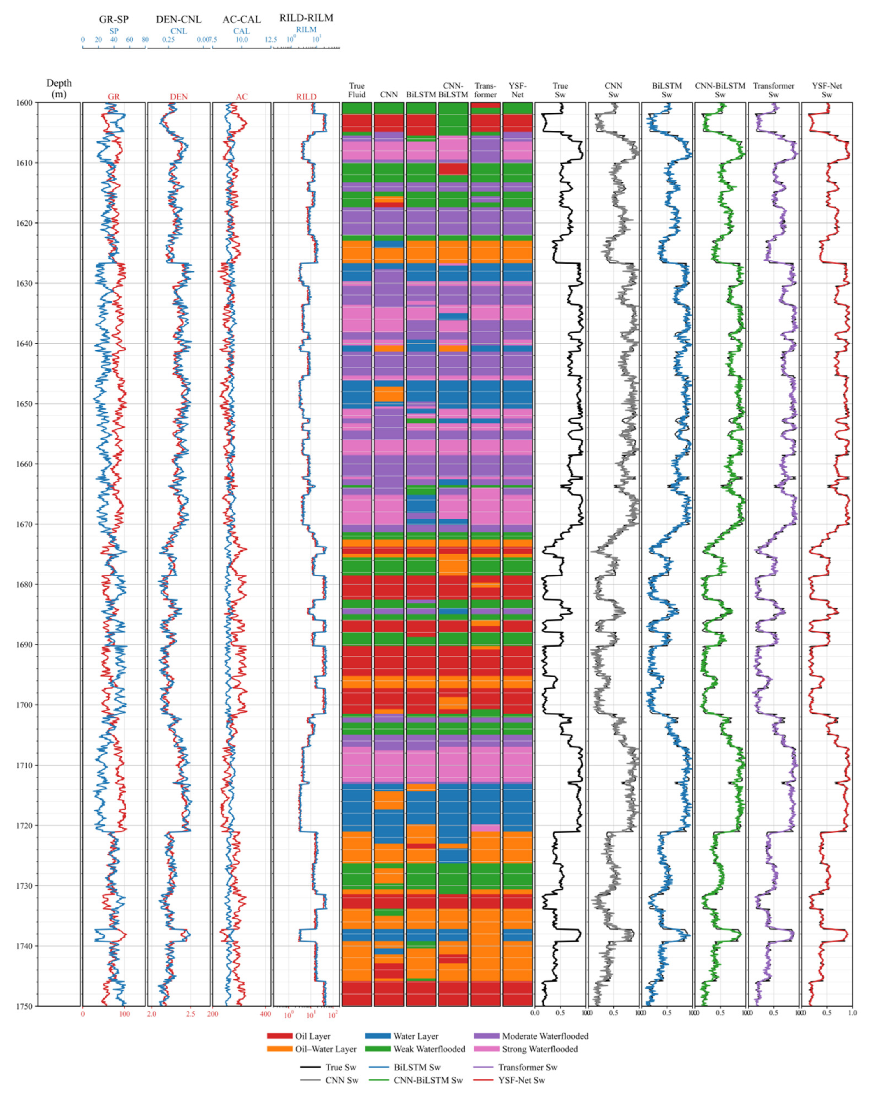
Figure 9 compares the logging curves, true fluid labels, predictions of different methods, and water-saturation curves for typical well intervals. For fluid identification, CNN and BiLSTM tend to produce discontinuous predictions and boundary drift in thin layers and transition zones. The CNN-BiLSTM and Transformer better recover the main fluid intervals, but local deviations still occur in thin beds and near the boundaries between oil–water layers and adjacent water-flooded layers. In contrast, the YSF-Net produces prediction bands that are most consistent with the true labels, showing better boundary positioning, thin-bed continuity, and transition-interval integrity. For water-saturation prediction, the YSF-Net follows the true curve more closely in both overall trend and local variations, especially in intervals with abrupt changes. These well-interval results further demonstrate that YSF-Net not only achieves a better statistical performance but also provides interpretation results that are more consistent with geological understanding in practical logging sections.

Figure 9. Comprehensive comparison of logging curves, fluid identification, and water saturation in typical well intervals.

4.6. Engineering Application Workflow, Uncertainty, and Validation

For field deployment, the YSF-Net follows a streamlined workflow. Conventional logs are first preprocessed through quality control, depth matching, outlier correction, robust standardization, and missing-mask construction. Reservoir-prior parameters, including shale volume, porosity, and permeability, are then calculated using regional interpretation criteria. Sliding-window samples are generated along the depth and input into the trained model, which simultaneously outputs six-class reservoir-fluid labels and continuous S_w curves. The results are finally integrated with production data, stratigraphic information, and expert interpretation for reservoir evaluation.

Prediction reliability was assessed using classification probability margins and S_w residuals. High-uncertainty samples are mainly concentrated in oil–water and water-flooding transition zones, consistent with the confusion-matrix and boundary analyses, indicating that the uncertainty is geologically interpretable. Model reliability was further verified through well-based splitting, five-fold cross-validation, direct cross-well testing, and typical well-interval comparison.

Overall, this study contributes to reservoir-fluid interpretation in three aspects. First, it demonstrates that reservoir-fluid identification and S_w prediction should be jointly modeled because fluid-state boundaries and saturation variations are physically coupled. Second, it shows that regional stratigraphic constraints and reservoir-prior parameters help reduce uncertainty in heterogeneous reservoirs with different depositional backgrounds. Third, it confirms that physical consistency constraints improve the geological rationality of S_w prediction, especially in thin beds, transition zones, and mixed-deposition reservoirs. Therefore, the YSF-Net provides an integrated and practical workflow for converting conventional well-log data into interpretable reservoir-fluid labels and continuous saturation profiles.

5. Conclusions

(1) This study proposed the YSF-Net for joint reservoir-fluid identification and water-saturation prediction in the Youshashan Oilfield. By integrating multi-log sequence representation, regional stratigraphic constraints, reservoir-prior parameters, multi-task learning, and physical consistency constraints, the model enables six-class reservoir-fluid identification and continuous S_w prediction within a unified framework.

(2) YSF-Net achieved the best overall performance among all compared models. Its Accuracy, Macro-F1, and Macro-AUC reached 0.926, 0.913, and 0.968, respectively, while the S_w RMSE and MAE decreased to 0.061 and 0.047 and S_w R² increased to 0.947. Compared with the Transformer, YSF-Net improved the Accuracy and Macro-F1 by 1.3 and 1.2 percentage points, respectively, and reduced S_w RMSE by 0.007.

(3) Ablation and transition-boundary analyses verified the effectiveness of the key components. Removing reservoir-prior inputs caused the largest performance decline, reducing Accuracy to 0.898 and increasing S_w RMSE to 0.079. Removing the physical constraint increased the S_w RMSE from 0.061 to 0.074, indicating its main role in improving S_w prediction reliability. YSF-Net also maintained stable discrimination in oil–water and water-flooding transition zones.

(4) Cross-well and reservoir-type tests demonstrated the applicability of the YSF-Net to heterogeneous reservoirs. In direct cross-well testing without fine-tuning, the YSF-Net achieved a Cross-well Accuracy of 0.918, a Cross-well Macro-F1 of 0.904, and a Cross-well S_w RMSE of 0.064. Across delta-front clastic, distal front transitional, and mixed-deposition reservoirs, the Accuracy remained approximately 0.90 or higher. These results indicate that the YSF-Net provides an efficient and geologically consistent tool for multi-well reservoir-fluid interpretation, water-flooding evaluation, and dynamic reservoir management.

References

- Adeogun, O.Y.; Abdulwaheed, M.O.; Adeoti, L.; Allo, O.J.; Fasakin, O.O.; Okunowo, O.O. Machine learning approach in predicting water saturation using well data at “TM” Niger Delta. Sci. Afr. 2025, 27, e02596. [Google Scholar] [CrossRef]
- Akbari, A.; Ranjbar, A.; Kazemzadeh, Y.; Martyushev, D.A. Enhanced water saturation estimation in hydrocarbon reservoirs using machine learning. Sci. Rep. 2025, 15, 29846. [Google Scholar] [CrossRef]
- Al-Fakih, A.; Koeshidayatullah, A.; Mukerji, T.; Al-Azani, S.; Kaka, S.I. Well log data generation and imputation using sequence based generative adversarial networks. Sci. Rep. 2025, 15, 11000. [Google Scholar] [CrossRef]
- Al-Mudhafar, W.J. Integrating well log interpretations for lithofacies classification and permeability modeling through advanced machine learning algorithms. J. Pet. Explor. Prod. Technol. 2017, 7, 1023–1033. [Google Scholar] [CrossRef]
- Ballinas, M.R.; Bedle, H.; Devegowda, D. Supervised machine learning for discriminating fluid saturation and presence in subsurface reservoirs. J. Appl. Geophys. 2023, 217, 105192. [Google Scholar] [CrossRef]
- Bhattacharya, B.; Carr, T.R.; Pal, M. Comparison of supervised and unsupervised approaches for mudstone lithofacies classification: Case studies from the Bakken and Mahantango-Marcellus Shale, USA. J. Nat. Gas Sci. Eng. 2016, 33, 1119–1133. [Google Scholar] [CrossRef]
- Bhattacharya, B.; Mishra, S. Applications of machine learning for facies and fracture prediction using Bayesian network theory and random forest: Case studies from the Appalachian Basin, USA. J. Pet. Sci. Eng. 2018, 170, 1005–1017. [Google Scholar] [CrossRef]
- Bressan, T.S.; de Souza, M.K.; Girelli, T.J.; Junior, F.C. Evaluation of machine learning methods for lithology classification using geophysical data. Comput. Geosci. 2020, 139, 104475. [Google Scholar] [CrossRef]
- Deng, S.; Aldrich, C.; Liu, X.; Zhang, F. Explainability in reservoir well-logging evaluation: Comparison of variable importance analysis with Shapley value regression, SHAP and LIME. IFAC-PapersOnLine 2024, 58, 66–71. [Google Scholar] [CrossRef]
- Gohari Nezhad, A.; Emami Niri, M. Enhancing water saturation predictions from conventional well logs in a carbonate gas reservoir with a hybrid CNN-LSTM model. J. Pet. Explor. Prod. Technol. 2025, 15, 89. [Google Scholar] [CrossRef]
- Guo, J.; Ling, Z.; Xu, X.; Zhao, Y.; Yang, C.; Wei, B.; Zhang, Z.; Zhang, C.; Tang, X.; Chen, T.; et al. Saturation determination and fluid identification in carbonate rocks based on well logging data: A Middle Eastern case study. Processes 2023, 11, 1282. [Google Scholar] [CrossRef]
- Hadavimoghaddam, F.; Ostadhassan, M.; Sadri, M.A.; Bondarenko, T.; Chebyshev, I.; Semnani, A. Prediction of water saturation from well log data by machine learning algorithms: Boosting and super learner. J. Mar. Sci. Eng. 2021, 9, 666. [Google Scholar] [CrossRef]
- He, M.; Gu, H.; Wan, H. Log interpretation for lithology and fluid identification using deep neural network combined with MAHAKIL in a tight sandstone reservoir. J. Pet. Sci. Eng. 2020, 194, 107498. [Google Scholar] [CrossRef]
- Hu, X.; Meng, Q.; Guo, F.; Xie, J.; Hasi, E.; Wang, H.; Zhao, Y.; Wang, L.; Li, P.; Zhu, L.; et al. Deep learning algorithm-enabled sediment characterization techniques to determination of water saturation for tight gas carbonate reservoirs in Bohai Bay Basin, China. Sci. Rep. 2024, 14, 12179. [Google Scholar] [CrossRef]
- Hua, Y.; Gao, G.; He, D.; Wang, G.; Liu, W. Reservoir fluid identification based on multi-head attention with UMAP. Geoenergy Sci. Eng. 2024, 238, 212888. [Google Scholar] [CrossRef]
- Imamverdiyev, Y.; Sukhostat, L. Lithological facies classification using deep convolutional neural network. J. Pet. Sci. Eng. 2019, 174, 216–228. [Google Scholar] [CrossRef]
- Jiang, S.; Sun, P.; Lyu, F.; Zhu, S.; Zhou, R.; Li, B.; He, T.; Lin, Y.; Gao, Y.; Song, W.; et al. Machine learning (ML) for fluvial lithofacies identification from well logs: A hybrid classification model integrating lithofacies characteristics, logging data distributions, and ML models applicability. Geoenergy Sci. Eng. 2024, 233, 212587. [Google Scholar] [CrossRef]
- Khan, S.Q.; Kirmani, F.U.D. Applicability of deep neural networks for lithofacies classification from conventional well logs: An integrated approach. Pet. Res. 2024, 9, 393–408. [Google Scholar] [CrossRef]
- Kumar, T.; Arif, M.; Rao, G.S. Lithology prediction from well log data using machine learning techniques: A case study from Talcher coalfield, Eastern India. J. Appl. Geophys. 2022, 199, 104605. [Google Scholar] [CrossRef]
- Li, H.; Chen, M.; Zhang, X.; Yang, B.; Zhao, B.; Li, X.; Wang, H. Reservoir fluid identification based on Bayesian-optimized SVM model. Processes 2025, 13, 369. [Google Scholar] [CrossRef]
- Li, Z.; Li, P.; Liu, Z.; Cui, Y. Single-well lithofacies identification based on logging response and convolutional neural network. J. Appl. Geophys. 2022, 207, 104865. [Google Scholar] [CrossRef]
- Li, Z.; Deng, S.; Hong, Y.; Wei, Z.; Cai, L. A novel hybrid CNN–SVM method for lithology identification in shale reservoirs based on logging measurements. J. Appl. Geophys. 2024, 223, 105346. [Google Scholar] [CrossRef]
- Liang, Y.; Zhang, B.; Wang, W.; Fang, S.; Zhang, Z.; Peng, L.; Zhang, Z. Deep learning-based fluid identification with residual vision transformer network (ResViTNet). Processes 2025, 13, 1707. [Google Scholar] [CrossRef]
- Liu, J.-J.; Liu, J.-C. Integrating deep learning and logging data analytics for lithofacies classification and 3D modeling of tight sandstone reservoirs. Geosci. Front. 2022, 13, 101311. [Google Scholar] [CrossRef]
- Luo, X.; Sun, J.; Zhang, J.; Liu, W. A new method based on multiresolution graph-based clustering for lithofacies analysis of well logging. Comput. Geosci. 2024, 28, 491–502. [Google Scholar] [CrossRef]
- Markovic, S.; Bryan, J.L.; Rezaee, R.; Turakhanov, A.; Cheremisin, A.; Kantzas, A.; Koroteev, D. Application of XGBoost model for in-situ water saturation determination in Canadian oil-sands by LF-NMR and density data. Sci. Rep. 2022, 12, 13984. [Google Scholar] [CrossRef]
- Miah, M.I.; Zendehboudi, S.; Ahmed, S. Log data-driven model and feature ranking for water saturation prediction using machine learning approach. J. Pet. Sci. Eng. 2020, 194, 107291. [Google Scholar] [CrossRef]
- Ren, X.; Hou, J.; Song, S.; Liu, Y.; Chen, D.; Wang, X.; Dou, L. Lithology identification using well logs: A method by integrating artificial neural networks and sedimentary patterns. J. Pet. Sci. Eng. 2019, 182, 106336. [Google Scholar] [CrossRef]
- Rezaei Mirghaed, B.; Dehghan Monfared, A.; Ranjbar, A. Enhanced petrophysical evaluation through machine learning and well logging data in an Iranian oil field. Sci. Rep. 2024, 14, 28941. [Google Scholar] [CrossRef] [PubMed]
- Singh Sandhu, S.K. Uncertainty quantification of well log predictions. Interpretation 2026, 14, B31–B38. [Google Scholar] [CrossRef]
- Wang, W.; Qu, L.; Yue, D.; Li, W.; Liu, J.; Jin, W.; Fu, J.; Zhang, J.; Chen, D.; Wang, Q.; et al. Integrated artificial intelligence approach for well-log fluid identification in dual-medium tight sandstone gas reservoirs. Front. Earth Sci. 2025, 13, 1591110. [Google Scholar] [CrossRef]
- Wang, Z.; Cai, Y.; Liu, D.; Lu, J.; Qiu, F.; Hu, J.; Li, Z.; Gamage, R.P. A review of machine learning applications to geophysical logging inversion of unconventional gas reservoir parameters. Earth-Sci. Rev. 2024, 258, 104969. [Google Scholar] [CrossRef]
- Xie, Y.; Zhu, C.; Zhou, W.; Li, Z.; Liu, X.; Tu, M. Evaluation of machine learning methods for formation lithology identification: A comparison of tuning processes and model performances. J. Pet. Sci. Eng. 2018, 160, 182–193. [Google Scholar] [CrossRef]
- Yang, H.; Chong, Z.; Xiong, L.; Xiong, W.; Lin, G.; Huang, K.; Zhang, W. Research on prediction method of well logging reservoir parameters based on Multi-TransFKAN model. Sci. Rep. 2025, 15, 18057. [Google Scholar] [CrossRef] [PubMed]
- Yang, X.; Zhang, C.; Zhao, S.; Zhou, T.; Zhang, D.; Shi, Z.; Liu, S.; Jiang, R.; Yin, M.; Wang, G.; et al. CLAP: Gas saturation prediction in shale gas reservoir using a cascaded convolutional neural network–long short-term memory model with attention mechanism. Processes 2023, 11, 2645. [Google Scholar] [CrossRef]
- Zeng, L.; Ren, W.; Shan, L. Attention-based bidirectional gated recurrent unit neural networks for well logs prediction and lithology identification. Neurocomputing 2020, 414, 153–171. [Google Scholar] [CrossRef]
- Zeng, L.; Ren, W.; Shan, L.; Huo, F. Well logging prediction and uncertainty analysis based on recurrent neural network with attention mechanism and Bayesian theory. J. Pet. Sci. Eng. 2022, 208, 109458. [Google Scholar] [CrossRef]
Disclaimer/Publisher’s Note: The statements, opinions and data contained in all publications are solely those of the individual author(s) and contributor(s) and not of MDPI and/or the editor(s). MDPI and/or the editor(s) disclaim responsibility for any injury to people or property resulting from any ideas, methods, instructions or products referred to in the content. |
© 2026 by the authors. Licensee MDPI, Basel, Switzerland. This article is an open access article distributed under the terms and conditions of the Creative Commons Attribution (CC BY) license.