


Abstract
This study proposes a multi-sensor time-series framework for estimating sugarcane planting Days After Planting (DAP) using Sentinel-1 synthetic aperture radar (SAR) and Sentinel-2 optical imagery in Phu Khiao District, Chaiyaphum Province, Thailand. The framework integrates vegetation indices, SAR backscatter, Dynamic Time Warping Barycenter Averaging (DBA), Derivative Dynamic Time Warping (DDTW), and stage-specific Ordinary Least Squares (OLS) calibration to estimate planting DAP and crop age. Sugarcane fields were first identified using a Random Forest classifier trained on combined multispectral and SAR features, achieving an Overall Accuracy of 88.5% and a Kappa coefficient of 0.82 for the optimal feature configuration. Multi-temporal vegetation index and SAR backscatter time series were then smoothed using Locally Weighted Scatterplot Smoothing (LOWESS) and aligned with phenological reference prototypes generated by DBA using DDTW. Stage-specific OLS models were subsequently applied to reduce systematic prediction bias. The calibrated framework achieved a coefficient of determination (R2) of 0.9970 and a root mean square error (RMSE) of 5.21 days, representing a substantial improvement over the uncalibrated DDTW estimates (R2 = 0.9953, RMSE = 7.00 days). DDTW alignment produced the highest accuracy during the grand growth stage (Stage 2), with normalized RMSE (NRMSE) ranging from 0.064 to 0.091 across individual features. Independent validation using 140 sugarcane plots from the 2024/2025 cropping season demonstrated the plausibility of the proposed framework, correctly identifying Stage 3 (sugar accumulation) growth for 98.6% of the plots and estimating a mean planting DAP of 267.06 ± 9.55 days. These findings demonstrate that the proposed framework provides an accurate and operational approach for estimating sugarcane planting dates from satellite time-series data, supporting crop age monitoring and harvest planning in tropical agricultural regions where field-based planting records are unavailable or incomplete.
1. Introduction
Sugarcane (Saccharum officinarum L.) is one of Thailand’s most important economic crops, serving as the primary raw material for the sugar industry and contributing substantially to agricultural production, rural livelihoods, and export revenue [1]. During the 2023/2024 production season, more than 11 million rai of sugarcane were cultivated nationwide, yielding over 82 million tons of cane and supporting the livelihoods of more than one million farmers [2]. Chaiyaphum Province is one of the country’s major production areas, with approximately 593,597 rai under cultivation and an annual production exceeding 5.88 million tons, corresponding to an average yield of 9.9 tons per rai [2].
Within the province, Phu Khieo District accounted for approximately 196,386 rai of sugarcane cultivation, representing 39.04% of the district area during the 2024/2025 production season [3]. The dominant cultivar is Khon Kaen 3, which is widely grown under rain-fed conditions from March to June and is well adapted to drought and high temperatures that promote sugar accumulation during the ripening stage [4]. Accurate information on sugarcane planting dates is fundamental for crop management throughout the production cycle. Key production indicators, including cultivated area, crop age, growth stage, and yield estimation, are required for harvest scheduling, Commercial Cane Sugar (CCS) assessment, procurement planning, and sugar mill operation management. Among these variables, the planting date, commonly expressed as Days After Planting (DAP), directly determines crop age and strongly influences sugar accumulation. CCS generally increases throughout the ripening period before declining as the crop becomes over-mature. Consequently, accurate estimation of planting DAP is essential for identifying the optimal harvest window and maximizing sugar production [5,6,7]. In practice, however, planting dates are typically obtained through field surveys, which are labor-intensive, time-consuming, and often incomplete or inaccurate, particularly in large production areas [8].
Because conventional field surveys are labor-intensive and often incomplete, remote sensing has emerged as an effective alternative for monitoring sugarcane production over large areas. Previous studies have successfully employed optical satellite imagery and vegetation indices, including NDVI, MSI, and SAVI, for sugarcane mapping and crop condition assessment [9]. However, optical imagery alone remains highly susceptible to cloud contamination during the rainy season, resulting in discontinuous time series precisely when sugarcane experiences rapid phenological development [10,11,12]. To overcome this limitation, Sentinel-1 Synthetic Aperture Radar (SAR) has received increasing attention because microwave signals penetrate cloud cover and provide weather-independent observations throughout the growing season. Recent studies have demonstrated that integrating Sentinel-1 SAR with Sentinel-2 optical imagery substantially improves sugarcane mapping accuracy compared with single-sensor approaches [13,14,15].
Beyond mapping cultivated areas, increasing attention has been directed toward estimating planting dates and crop phenology at the individual plot level, particularly within Thailand’s fragmented smallholder farming systems. Existing satellite-based approaches for estimating planting DAP generally fall into three categories. Threshold-based methods identify planting dates when vegetation indices exceed predefined thresholds [16,17], whereas function-fitting approaches estimate phenological transitions by fitting mathematical growth curves to time-series observations [16,17]. More recently, deep learning approaches such as Long Short-Term Memory (LSTM) [18,19] networks have demonstrated the ability to model complex temporal dynamics. Nevertheless, these approaches require substantial numbers of reference planting dates for model calibration and generally perform best with complete and continuous time-series observations. Their applicability is therefore limited in tropical environments where cloud contamination, irregular observations, and incomplete field records are common.
Dynamic Time Warping (DTW) offers an alternative paradigm by aligning temporal patterns directly rather than relying on absolute observation dates. An important advantage of DTW-based approaches is their ability to identify phenological similarity despite temporal shifts, thereby reducing dependence on known planting dates. Maus et al. (2016) introduced Time-Weighted Dynamic Time Warping (TWDTW), which incorporates seasonal constraints into temporal alignment, while Ye et al. (2023) demonstrated that Derivative Dynamic Time Warping (DDTW) applied to Sentinel-2 NDVI time series predicted multiple maize phenological stages with an RMSE below six days, outperforming conventional DTW and function-fitting approaches [20,21].
Despite these advances, several important challenges remain. First, DDTW has rarely been applied to plot-level sugarcane planting DAP estimation. Second, most existing studies rely primarily on optical imagery or single-sensor observations, limiting the temporal continuity of phenological monitoring under tropical cloud conditions. Third, the temporal transferability of DDTW-based models across different growing seasons has not been systematically evaluated, despite its importance for operational crop monitoring [21,22]. Collectively, these limitations restrict the operational application of time-series phenology models for large-scale sugarcane monitoring [21,22].
Although DDTW effectively aligns phenological trajectories, the temporal offsets obtained from sequence alignment do not necessarily correspond directly to actual planting dates. Consequently, an additional calibration step may be required to translate DDTW-derived temporal offsets into more reliable planting DAP estimates. Several calibration approaches, including polynomial regression and machine learning algorithms, have been proposed for this purpose. However, these methods generally require either more complex model specification or larger training datasets. In contrast, simple linear calibration models offer advantages in terms of interpretability, computational efficiency, and applicability when only a limited number of reference planting dates are available [23]. Therefore, incorporating a statistical calibration step into the DDTW framework has the potential to reduce systematic prediction bias and improve the reliability of planting date estimation.
To address these challenges, this study develops a multi-sensor temporal alignment framework that combines Sentinel-1 SAR, Sentinel-2 optical imagery, Dynamic Time Warping Barycenter Averaging (DBA), Derivative Dynamic Time Warping (DDTW), and stage-specific Ordinary Least Squares [24] calibration for plot-level estimation of sugarcane planting. DBA is first employed to construct representative phenological prototypes from plots with known planting dates, after which DDTW aligns temporal trajectories from target fields to estimate planting DAP. Finally, stage-specific OLS models are applied to reduce systematic prediction bias. By integrating multi-sensor observations with temporal pattern matching and statistical calibration, the proposed framework enables robust plot-level planting date estimation without requiring complete field records. The resulting information can support harvest scheduling, sugar mill logistics, and crop management while providing a transferable methodology for large-scale sugarcane monitoring in tropical agricultural regions.
2. Study Area and Dataset
2.1. Study Area
The study was conducted in Phu Khiao District, Chaiyaphum Province, northeastern Thailand (Figure 1). The district covers approximately 801.93 km2 (6.27% of the provincial area) and is geographically bounded by 16.1682–16.5115° N and 101.9610–102.3554° E. During the 2024/2025 production season, Phu Khiao contained approximately 196,386 rai of sugarcane, accounting for 39.04% of the total sugarcane cultivation area in Chaiyaphum Province. Sugarcane is the district’s second most important economic crop after rice and is cultivated extensively because of the proximity of several sugar processing facilities. The dominant cultivar is Khon Kaen 3, which is widely adopted because of its drought tolerance, vigorous tillering, high sugar content, and adaptability to former paddy fields [4]. Sugarcane production is predominantly rain-fed, with planting typically occurring between May and June at the onset of the rainy season. While frequent cloud cover during the rainy season limits the availability of optical satellite observations, relatively dry and warm conditions during the ripening period favor sugar accumulation. These environmental characteristics make Phu Khiao District an appropriate test site for evaluating multi-sensor time-series approaches. The combination of seasonal cloud contamination, rain-fed cultivation, and variable planting dates provides a challenging yet representative environment for assessing the robustness of the proposed framework for estimating sugarcane planting Days After Planting (DAP).
Figure 1.
Location of the study area in Phu Khiao District, Chaiyaphum Province, northeastern Thailand, showing the district boundary and the distribution of sugarcane cultivation areas.
Sugarcane cultivation in Thailand follows distinct planting calendars that are primarily determined by regional rainfall regimes and water availability (Figure 2). Three principal production systems are recognized. Irrigated (off-season) cane is planted between January and March using supplementary irrigation before the onset of the rainy season. Early rainfed cane is established from April to May and relies on seasonal rainfall, whereas late rainfed (October) cane is planted between October and December using residual soil moisture following the wet season. Although planting periods differ among these production systems, harvesting generally occurs between December and March to coincide with the annual crushing season of sugar mills.
Figure 2.
Typical sugarcane crop calendar in Thailand, illustrating the planting periods of the three principal production systems and the typical harvesting season. Green represents irrigated (off-season) planting during January–March, purple represents early rainy-season planting during April–May, orange represents late rainy-season (October cane) planting during October–December, and yellow represents the typical harvesting season during December–March.
Phu Khiao District represents a typical irrigated sugarcane production area in northeastern Thailand. Farmers generally establish sugarcane during March and harvest the crop after approximately 12 months, resulting in a relatively consistent annual production cycle. As a result, the dominant planting cycle in this district follows a relatively uniform annual pattern, with planting in March and harvesting between December and March of the following year, aligning with the regional mill crushing schedule. The district is dominated by the Khon Kaen 3 cultivar, which is well adapted to drought-prone conditions and sandy loam soils but has limited tolerance to prolonged waterlogging [4]. This relatively uniform planting schedule, together with the seasonal cloud cover characteristic of the rainy season, provides an appropriate environment for evaluating satellite-based estimation of sugarcane planting Days After Planting (DAP).
2.2. Dataset
2.2.1. Satellite Imagery
- Sentinel-2 Level-2A multispectral imagery was obtained from the Copernicus Data Space Ecosystem and processed using Google Earth Engine [25]. The Level-2A products provide atmospherically corrected surface reflectance suitable for quantitative vegetation analysis. Images acquired between 1 and 4 December 2025, corresponding to the pre-harvest stage of sugarcane, were selected to characterize crop conditions during the ripening period. Only scenes with cloud cover below 10% were included to minimize atmospheric contamination. Surface reflectance values were rescaled following the Copernicus product specification before calculating vegetation indices used for sugarcane mapping and time-series analysis [26].
- Sentinel-1 Ground Range Detected (GRD) imagery acquired in Interferometric Wide Swath (IW) mode was used to complement the optical observations. Dual-polarization backscatter coefficients (VV and VH) were extracted to characterize crop structure and canopy moisture under all-weather conditions. Standard preprocessing, including radiometric calibration, speckle filtering, terrain correction, and conversion to sigma nought (σ0) in decibel (dB), was performed within Google Earth Engine following the recommended Sentinel-1 processing workflow [25]. To ensure temporal consistency with the Sentinel-2 observations, Sentinel-1 images acquired during the corresponding pre-harvest period were aggregated using a median compositing approach [27]. Median compositing reduced residual speckle noise and short-term variability while preserving representative backscatter characteristics. The resulting Sentinel-1 SAR backscatter and Sentinel-2 optical observations were subsequently integrated to generate multi-sensor features for sugarcane classification and planting Days After Planting (DAP) estimation [22].
2.2.2. Reference Field Plots
The reference dataset consisted of 100 sugarcane field plots collected during the 2023/2024 cropping season. Each plot included a verified planting date, a unique plot identifier, and polygon boundaries for extracting satellite-derived time-series observations. The field data were obtained and served as the reference dataset for model development.
For each reference plot, multi-sensor time-series observations from Sentinel-1 SAR and Sentinel-2 optical imagery were extracted from 1 December 2023 to 31 December 2024, covering the pre-planting period, the complete crop growth cycle, and the pre-harvest stage. Verified planting dates ranged from December of the previous calendar year (DAP 335) to March of the following year (DAP 90), representing the range of planting schedules within the study area. These reference plots were used for model development and internal validation through five-fold cross-validation.
2.2.3. Independent Validation Plots
An independent validation dataset consisting of 140 sugarcane plots was established for evaluating the temporal transferability of the proposed framework during the 2024/2025 cropping season. The plots were selected from sugarcane fields identified using a Random Forest classification model [28] followed by stratified random sampling to ensure representative spatial coverage across the study area.
For each validation plot, multi-sensor time-series observations from Sentinel-1 SAR and Sentinel-2 optical imagery were extracted from 16 February 2025 to 14 February 2026, covering approximately one complete crop growth cycle. The extraction period was determined based on field surveys, which indicated that sugarcane planting in the study area generally begins in March. Consequently, data acquisition commenced in mid-February to capture pre-planting baseline conditions and continued through crop maturity. This independent dataset was used exclusively to evaluate the temporal transferability and prediction performance of the proposed DAP estimation framework.
3. Methods
This study proposes a multi-sensor framework for estimating sugarcane planting Days After Planting (DAP) from satellite time-series observations without requiring prior knowledge of planting dates. The overall workflow consists of five major components: (1) sugarcane field identification, (2) multi-sensor time-series construction and smoothing, (3) phenological prototype generation and temporal alignment, (4) stage-specific DAP calibration, and (5) spatial prediction of planting DAP for fields with unknown planting dates (Figure 3).
Figure 3.
Overall workflow of the proposed framework for sugarcane planting Days After Planting (DAP) estimation, comprising (1) sugarcane area mapping, (2) multi-sensor time-series processing and initial DAP estimation, (3) stage-specific DAP calibration using Ordinary Least Squares (OLS) and (4) spatial prediction of planting DAP for fields with unknown planting dates.
First, sugarcane fields were identified from Sentinel-1 SAR and Sentinel-2 optical imagery using a Random Forest classifier. Multi-sensor time-series observations were then extracted for each field and smoothed data to reduce noise while preserving phenological characteristics. Representative phenological prototypes were subsequently generated using Dynamic Time Warping Barycenter Averaging (DBA), and Derivative Dynamic Time Warping (DDTW) was employed to align each target time series with the corresponding prototype and obtain an initial estimate of planting DAP.
To reduce systematic prediction bias, Ordinary Least Squares (OLS) regression models were developed separately for individual growth stages and applied to calibrate the initial DDTW-derived DAP estimates. The calibrated predictions were then used to estimate crop age and generate a spatially explicit planting DAP map for sugarcane fields during the 2024/2025 cropping season.
3.1. Sugarcane Area Classification
3.1.1. Satellite Preprocessing
Satellite image preprocessing was performed using the Google Earth Engine (GEE) cloud computing platform. Sentinel-2 Level-2A surface reflectance imagery was used as the primary optical dataset, while Sentinel-1 Ground Range Detected (GRD) imagery in Interferometric Wide Swath (IW) mode provided complementary Synthetic Aperture Radar (SAR) observations. Sentinel-1 data were preprocessed using radiometric calibration, terrain correction, and conversion to sigma nought (σ0) backscatter coefficients, followed by speckle reduction using a focal mean filter. Sentinel-1 and Sentinel-2 images acquired during the same observation period were combined to minimize temporal inconsistencies and provide complementary structural and spectral information for sugarcane classification [29].
3.1.2. Feature Extraction
Eight remote sensing features were extracted from the preprocessed satellite imagery, including six vegetation indices derived from Sentinel-2 (NDVI, GNDVI, MSI, CIred-edge, SAVI, and SAREI) together with Sentinel-1 VV and VH backscatter coefficients. These features collectively characterize vegetation vigor, chlorophyll content, canopy moisture, soil background effects, and crop structural properties. The mathematical formulations, spectral bands, and functional descriptions of each feature are summarized in Table 1.
Table 1.
Spectral and SAR features used for sugarcane classification.
The vegetation indices and SAR backscatter features listed in Table 1 were subsequently extracted for each reference plot using polygon-based zonal statistics and used as predictor variables for sugarcane classification. Mean values were calculated to represent field-level conditions while minimizing within-plot variability and mixed-pixel effects. Prior to model development, feature distributions were examined using boxplots, and outliers were identified using the interquartile range (IQR) criterion (1.5 × IQR). Detected outliers were removed to improve class consistency and reduce noise in the training dataset [36].
To evaluate the relative contribution of optical and radar information to sugarcane classification, four feature-set configurations were subsequently constructed and compared (Table 2).
Table 2.
Feature-set configurations for sugarcane classification.
3.1.3. Random Forest Classification
Sugarcane areas were classified using the Random Forest algorithm [37] implemented with 100 decision trees. Six land-cover classes were considered, including Agricultural, Forest, Miscellaneous, Urban and built-up, water, and Sugarcane. The classifier was trained using an integrated feature space consisting of optical bands, vegetation indices, and SAR backscatter to exploit complementary information on vegetation physiology, moisture status, and canopy structure.
The reference dataset consisted of 400 field polygons, from which 54,304-pixel samples were extracted. The dataset was divided at the field-polygon level into training (80%; 320 polygons) and testing (20%; 80 polygons) subsets. All pixel samples from the same field polygon were retained within the same subset to prevent spatial autocorrelation and information leakage between the training and testing datasets.
The trained Random Forest model was subsequently applied to classify the entire study area, producing a sugarcane distribution map used for selecting target plots for subsequent DAP estimation.
The Random Forest classification was performed using the December 2025 Sentinel-1/Sentinel-2 image composite. This image composite was used exclusively for land-cover classification and was independent of the 2023/2024 reference time series used to develop the DDTW-based phenological model and the 2024/2025 target time series (February 2025–February 2026) used for planting Days After Planting (DAP) estimation. These datasets served different objectives and were processed independently throughout the study.
3.1.4. Accuracy Assessment
Classification performance was evaluated using an independent validation dataset and a confusion matrix. Overall Accuracy (OA), Producer’s Accuracy (PA), User’s Accuracy (UA), F1-score, and the Kappa coefficient were calculated to quantify classification performance. In addition, the four feature-set configurations were compared to evaluate the contribution of optical and SAR observations to sugarcane discrimination.
Ground reference data were collected during two field campaigns conducted between 25–28 November 2025 and 17–19 December 2025. A total of 400 validation samples were obtained using stratified random sampling based on land-cover classes to ensure representative sampling across the study area.
3.2. DDTW Prototype Generation
3.2.1. Reference Dataset
The reference dataset comprised 100 sugarcane plots collected during the 2023/2024 cropping season, each with a verified planting date (Section 2.2.2). The verified planting dates were used to transform the original calendar dates into a crop-age coordinate system, where the planting date was defined as DAP = 0. Consequently, negative DAP values represent the pre-planting period, whereas positive DAP values correspond to crop age after planting.
The reference plots covered all four major sugarcane growth stages to ensure that the resulting phenological prototypes represented the complete crop development cycle. For each plot, multi-sensor time-series extraction commenced five days before planting (DAP = −5) to capture baseline conditions prior to crop emergence. These aligned time series subsequently served as the input for prototype construction using Dynamic Time Warping Barycenter Averaging (DBA) and for the calibration of the stage-specific Ordinary Least Squares (OLS) models.
3.2.2. Multi-Sensor Time-Series Extraction
Multi-sensor time-series observations were extracted for each reference plot, comprising six vegetation indices derived from Sentinel-2 imagery together with Sentinel-1 VV and VH backscatter features. For each acquisition date, mean feature values were calculated using polygon-based zonal statistics, resulting in a three-dimensional dataset consisting of plots × acquisition dates × features.
The extraction period extended from 1 December 2023 to 31 December 2024, encompassing the earliest planting dates, the complete crop growth cycle, and the pre-harvest stage for all reference plots. This common observation window ensured that baseline conditions prior to planting were captured for every plot and provided a consistent temporal framework for subsequent transformation to the crop-age (DAP) coordinate system and prototype construction using Dynamic Time Warping Barycenter Averaging (DBA).
3.2.3. Time-Series Preprocessing
The extracted Sentinel-1 and Sentinel-2 time series were preprocessed prior to prototype construction to reduce data gaps and suppress high-frequency noise. Temporal discontinuities arose primarily from the revisit intervals of the satellite sensors and cloud contamination during the rainy season.
The preprocessing workflow consisted of five sequential steps. First, the analysis period was restricted to DAP 0–330, corresponding to the active sugarcane growing season. Second, observations with valid data from fewer than 70% of the reference plots were removed to avoid constructing prototypes from sparsely sampled dates. Third, plots containing fewer than 12 valid observations were excluded to ensure sufficient temporal density for reliable interpolation and smoothing. Fourth, missing observations within the remaining time series were reconstructed using linear interpolation, while leading and trailing gaps were completed using forward and backward filling to generate continuous temporal trajectories. Finally, the reconstructed time series were smoothed using Locally Weighted Scatterplot Smoothing (LOWESS) to reduce residual noise while preserving the underlying phenological trends [38,39,40].
LOWESS is a non-parametric local regression method that estimates the fitted value at each observation by performing weighted least-squares regression within a local neighborhood [39]. Neighboring observations receive weights according to the tricube kernel function,
where Wixi is the weight assigned to observation xi, and d(x) is the distance from the target observation to the most distant neighbor included in the local regression window. Observations closer to the target point receive greater weights, enabling LOWESS to preserve local phenological characteristics while suppressing short-term fluctuations. The resulting smoothed time series were subsequently used for prototype construction using DTW Barycenter Averaging (DBA).
ŷx = Σ Wixiyi
3.2.4. DAP Transformation
To enable direct comparison of phenological trajectories among plots with different planting dates, the calendar-based time axis was transformed into a crop-age coordinate system. For each plot, the planting date was defined as DAP = 0, and the temporal position of every observation was calculated as
where is the observation date and is the verified planting date. Consequently, DAP < 0 represents observations acquired before planting, whereas DAP > 0 corresponds to the number of days after planting (crop age). Expressing all time series in this common DAP coordinate system removed differences caused by variable planting dates and enabled direct construction of representative phenological prototypes using DTW Barycenter Averaging (DBA).
3.2.5. Prototype Construction Using DBA
Following transformation to the crop-age (DAP) coordinate system, a representative phenological prototype was constructed for each of the eight remote sensing features using DTW Barycenter Averaging (DBA). The resulting prototype represents the average temporal trajectory of sugarcane development and serves as the reference pattern for subsequent DDTW-based planting DAP estimation [41].
Prior to prototype construction, each time series was standardized using mean–variance normalization to remove differences in numerical scale among the vegetation indices and SAR backscatter features. DBA was then applied to the normalized time series to estimate a prototype that minimizes the cumulative Dynamic Time Warping distance between the prototype and all reference sequences. This procedure preserves characteristic phenological patterns while accommodating local temporal variability among individual plots [42].
After prototype estimation, the normalized prototype was transformed back to the original measurement scale of each feature using the corresponding mean and standard deviation of the training dataset. To suppress residual artifacts introduced during the averaging process, a two-stage post-processing procedure was applied consisting of (1) median filtering to remove isolated spikes and (2) mild LOWESS to preserve the overall phenological trajectory while reducing high-frequency fluctuations.
Finally, the representativeness of each prototype was evaluated by calculating the Root Mean Squared Error (RMSE) between the prototype and every reference time series. Comparable RMSE values obtained before and after post-smoothing indicated that the smoothing procedure preserved the original phenological characteristics while reducing local noise. The final output of this step consisted of eight fixed phenological prototypes, which were subsequently used as reference templates for DDTW-based planting DAP estimation.
3.3. DDTW-Based DAP Estimation
3.3.1. Local Normalization and Derivative Transformation
Prior to temporal alignment, each plot-level time series and the corresponding reference prototype were independently standardized using Z-score normalization to remove differences in baseline magnitude caused by local environmental conditions. This normalization allows the alignment process to focus on temporal patterns rather than absolute signal values.
where is the original observation, is the mean of the time series, and is the corresponding standard deviation.
Following normalization, both the plot and prototype time series were transformed into derivative space. The first derivative was estimated using the central-difference approximation described by [43] and subsequently smoothed using a five-point moving average to suppress high-frequency fluctuations while preserving the underlying phenological transitions. This preprocessing step improves the stability of temporal alignment by reducing the influence of residual atmospheric and sensor noise commonly observed in satellite time-series data.
3.3.2. DDTW Alignment and DAP Estimation
DAP was estimated using Derivative Dynamic Time Warping (DDTW), in which Dynamic Time Warping is applied to the derivative representations of the query and reference time series [43],
where Q and C denote the query and prototype time series, respectively, and dQ and dC are their corresponding first-order derivatives.
Temporal alignment was performed using Dynamic Time Warping with a [44] constraint window of one day to restrict excessive temporal warping after transformation to the crop-age coordinate system. The resulting warping path establishes the correspondence between observations in the query series and positions along the reference prototype [44,45].
The aligned prototype positions were subsequently mapped back to crop-age values using linear interpolation, yielding an estimated planting DAP for every observation. This procedure was independently applied to each of the six vegetation indices and two SAR backscatter features, resulting in eight DAP estimates for each plot. These multi-feature DAP estimates were subsequently used as predictor variables in the stage-specific calibration model.
3.3.3. Stage-Specific Accuracy Assessment
The performance of the DDTW-based DAP estimation was evaluated separately for each sugarcane growth stage (Table 3). Estimated DAP values were compared with the corresponding reference planting DAP, and estimation accuracy was quantified using Root Mean Squared Error (RMSE) and Normalized Root Mean Squared Error (NRMSE). Stage-specific evaluation was performed to assess how DDTW accuracy varied throughout the sugarcane growth cycle.
Table 3.
Growth-stage classification used for stage-specific DDTW evaluation.
3.4. Stage-Specific OLS Calibration
Following DDTW-based crop-age estimation, stage-specific Ordinary Least Squares (OLS) regression models were developed to calibrate the DDTW-derived DAP estimates [23,46]. Separate regression models were fitted for each of the four sugarcane growth stages because the relative contribution of optical vegetation indices and SAR backscatter features varies throughout crop development.
During model development, observations were assigned to the corresponding growth stage according to their reference DAP. Only observations whose reference DAP fell within the predefined range of each growth stage were included during model fitting, and a minimum of 50 observations was required for each stage to ensure statistically stable estimation of the regression coefficients.
During prediction, the appropriate stage-specific OLS calibration equation was selected using the median of the eight DDTW-derived age estimates (six vegetation indices and two SAR variables). The resulting median DAP was used to assign each observation to one of the four predefined growth stages (Stage 1: 0–30 days, Stage 2: 31–170 days, Stage 3: 171–295 days, and Stage 4: 296–330 days), after which the corresponding stage-specific OLS calibration equation was applied. When the individual index-derived age estimates spanned multiple growth stages, the median estimated DAP was used as the criterion for stage assignment because it preserved the continuous nature of crop-age estimation while reducing disagreement among the individual indices. A voting-based approach was not adopted because it would reduce continuous age estimates to discrete stage labels and potentially discard information regarding the proximity of the predicted DAP to stage boundaries.
In addition to the observation-level evaluation, a plot-level accuracy assessment was performed using the reference plots as the independent sampling units. For each reference plot, the daily predicted DAP values within each growth stage were aggregated using the median predicted DAP, and one aggregated estimate was retained for each plot. Plot-level RMSE, MAE, mean bias, and 95% confidence intervals were then calculated using these aggregated estimates to avoid inflating predictive performance through repeated daily observations from the same reference plot.
To examine whether the calibration equations exhibited evidence of severe overfitting, an additional five-fold Group K-Fold analysis was conducted as a supplementary diagnostic assessment. All daily observations belonging to the same reference plot were retained within the same fold to avoid splitting repeated observations between the training and validation subsets. Within each fold, only the stage-specific OLS calibration models were fitted using the training plots and evaluated on the corresponding validation plots. This analysis was performed solely to assess the stability of the OLS calibration equations across different subsets of reference plots and was not intended as the primary validation framework of the proposed methodology. Therefore, the reported Group K-Fold results should be interpreted as a supplementary assessment of calibration robustness rather than an independent evaluation of the entire workflow, because the preprocessing procedures—including LOWESS parameter selection and smoothing, normalization, DBA prototype construction, and DDTW matching—were completed using the full reference dataset before fold separation.
To further evaluate the contribution of the proposed stage-specific calibration strategy, an additional baseline experiment was conducted using a global OLS model fitted across the complete crop-age range (DAP 0–330 days). The global model employed the same predictor variables as the proposed framework but estimated a single regression equation for all growth stages. Model performance was evaluated using the same plot-level evaluation protocol and the supplementary Group K-Fold diagnostic procedure described above to ensure a consistent comparison with the proposed stage-specific OLS models. Predictive performance was compared using plot-level RMSE, MAE, mean bias, and bootstrap-based 95% confidence intervals. Computational time required for model fitting and prediction was also recorded for comparison.
To further evaluate the statistical properties of the stage-specific OLS calibration models, additional regression diagnostics were performed for each growth stage. Pearson correlation coefficients were calculated to examine pairwise linear relationships among the predictor variables. Variance inflation factors (VIF) were used to quantify the degree of multicollinearity associated with individual predictors, whereas standardized condition numbers were calculated to assess the overall linear dependence among the predictor set. Regression coefficient standard errors were examined to characterize the uncertainty and stability of the estimated coefficients. Residual diagnostics included the Jarque–Bera and Shapiro–Wilk tests to assess departures from residual normality, the Breusch–Pagan test to evaluate heteroscedasticity, and the Durbin–Watson statistic to assess serial correlation in the residuals. These analyses were conducted to characterize the statistical behavior and stability of the fitted calibration models. Because the proposed OLS models were developed primarily for predictive calibration rather than interpretation of individual regression coefficients, the diagnostic results were used to identify potential violations of regression assumptions and to support appropriate interpretation of the model outputs rather than to guide variable selection or predictor elimination.
The calibrated planting DAP was estimated as
where denotes the calibrated planting Days After Planting, is the intercept, and − are regression coefficients estimated separately for each growth stage. The resulting calibrated DAP values were subsequently used for spatial prediction and independent validation.
3.5. Spatial Prediction of Planting Date
The calibrated planting Days After Planting (DAPpred) obtained from the stage-specific OLS models was assigned to each target sugarcane plot to produce a spatially explicit planting DAP map for the 2024/2025 cropping season. Each polygon was attributed with its predicted planting date, estimated crop age, assigned growth stage, and 10-day sub-stage.
Crop age for each satellite acquisition date was subsequently calculated as
where is the satellite observation date, is the predicted crop age obtained from the stage-specific OLS calibration, and is the estimated calendar planting date. When required, the estimated planting date was additionally expressed as calendar planting day-of-year, representing the sequential day of the corresponding calendar year.
3.6. Independent Field Plausibility Assessment
Model performance was evaluated at two complementary levels. For the reference dataset, predictive accuracy was quantified using the coefficient of determination (R2), Root Mean Squared Error (RMSE), and Normalized Root Mean Squared Error (NRMSE).
Because verified planting dates were unavailable for the independent 2024/2025 dataset, no quantitative accuracy assessment was performed. Instead, the stage-specific OLS calibration models developed from the 2023–2024 reference dataset were applied to 140 target sugarcane plots cultivated during the 2025 growing season, and a field survey was conducted during 25–28 November 2025 to qualitatively compare the predicted phenological stages with observable crop characteristics, including canopy height, canopy density, and lower-leaf senescence. This field investigation was designed as an independent plausibility assessment of the predicted growth stages rather than a quantitative validation of model performance.
4. Result
4.1. Sugarcane Classification
The Random Forest classifier successfully discriminated sugarcane from the other five land-cover classes using four different feature-set configurations (RGB, vegetation indices, vegetation indices combined with SAR, and SAR only). Classification performance was evaluated using an independent validation dataset based on the confusion matrix, from which Overall Accuracy (OA), Producer’s Accuracy (PA), User’s Accuracy (UA), F1-score, and the Kappa coefficient were derived. The confusion matrices for the four feature sets are presented in Table 4.
Table 4.
Confusion matrices for the four Random Forest feature-set configurations.
Among the four feature-set configurations, the integration of vegetation indices and Sentinel-1 SAR backscatter (VIs + SAR) achieved the highest classification performance. This approach correctly classified 202 of the 215 sugarcane validation samples, resulting in the highest Overall Accuracy (OA) of 88.5%, Kappa coefficient of 81.9%, and Producer’s Accuracy for sugarcane of 94.0% (Table 5). In contrast, the SAR-only feature set produced the lowest classification performance (OA = 55.3%; Kappa = 32.4%), with substantial confusion between sugarcane, agricultural land, and forest classes. These results indicate that integrating optical vegetation indices with SAR backscatter substantially improves sugarcane discrimination by combining complementary spectral and structural information.
Table 5.
Classification performance of the four feature-set configurations.
The spatial distribution of the classification results obtained from the four feature-set configurations is presented in Figure 4. Overall, the RGB and vegetation-index models produced similar land-cover patterns; however, both exhibited misclassification between sugarcane and other agricultural vegetation. The integration of Sentinel-1 SAR with vegetation indices generated cleaner field boundaries and reduced confusion between adjacent agricultural classes, particularly in areas with heterogeneous crop patterns. In contrast, the SAR-only model showed fragmented sugarcane patches and substantial confusion with agricultural and forest areas, reflecting the limited discriminative capability of radar backscatter when used without complementary spectral information.
Figure 4.
Comparison of land-cover classification maps produced by different methods. (A) Satellite Image, (B) RGB, (C) VIS, (D) VIS + SAR, (E) SAR. The circles highlight representative areas where the classification results differ among the methods.
Figure 4 presents the spatial comparison of land-cover classification maps produced using the four feature-set configurations. Consistent with the quantitative accuracy assessment (Table 5), the integration of vegetation indices and Sentinel-1 SAR backscatter generated the most spatially coherent classification. Sugarcane fields exhibited more homogeneous patches, clearer field boundaries, and reduced confusion with adjacent agricultural land and forest compared with the other feature sets.
The RGB and vegetation-index classifications showed noticeable improvements over the SAR-only model; however, isolated misclassified pixels and confusion between agricultural and built-up areas were still evident in several locations. In contrast, the SAR-only classification produced fragmented land-cover patterns with pronounced speckle noise, resulting in substantial confusion among sugarcane, agricultural land, and forest.
The highlighted regions in Figure 4 demonstrate that incorporating SAR backscatter effectively corrected several misclassified areas observed in the RGB and vegetation-index classifications while preserving the geometric characteristics of field boundaries. These spatial observations are consistent with the quantitative results, confirming that the combination of optical vegetation indices and SAR backscatter provides the most reliable feature set for sugarcane mapping in heterogeneous agricultural landscapes.
4.2. DAP Estimation
4.2.1. Gap Filling and LOWESS
LOWESS effectively reduced short-term fluctuations caused by irregular satellite observations and atmospheric noise while preserving the seasonal growth trajectory of sugarcane. Representative examples of the smoothed Sentinel-2 NDVI (optical) and Sentinel-1 VH backscatter (SAR) time series are presented in Figure 5. During the rainy season (DAP 150–250), the Sentinel-2 NDVI time series contained substantial gaps and increased variability due to persistent cloud contamination, resulting in reduced observation frequency and greater uncertainty in the reconstructed trajectory. In contrast, the Sentinel-1 VH backscatter exhibited a more continuous and consistent temporal pattern because SAR observations are largely unaffected by cloud cover. These complementary characteristics highlight the importance of integrating optical and SAR data for continuous phenological monitoring in tropical agricultural regions.
Figure 5.
Examples of LOWESS applied to Sentinel-2 NDVI (a) and Sentinel-1 VH backscatter (b). Grey points represent the original observations, whereas the red curves indicate the LOWESS-smoothed time series.
4.2.2. Constructed DBA Prototypes
DTW Barycenter Averaging (DBA) generated representative phenological prototypes for the eight remote sensing features using the time-series observations from the 100 reference sugarcane plots (Figure 6). Overall, the DBA-derived curves closely followed the central tendency of the individual plot trajectories while substantially reducing inter-plot temporal variability.
Figure 6.
DBA-derived phenological prototypes for the eight remote sensing features. Grey lines represent individual plot time series (n = 100), while the red line denotes the representative prototype generated using DTW Barycenter Averaging (DBA).
The optical vegetation indices (NDVI, GNDVI, SAVI, CIred-edge, and SAREI) exhibited similar seasonal trajectories characterized by two prominent phenological maxima occurring approximately at DAP 80–100 and DAP 220–250. In contrast, the Moisture Stress Index (MSI) displayed an inverse seasonal pattern, decreasing during the rapid growth stage before gradually increasing toward crop maturity. The Sentinel-1 SAR backscatter features (VV and VH) showed comparatively smoother temporal trajectories with a broad maximum around DAP 170–220, reflecting gradual changes in canopy structure and biomass throughout the growing season.
The representativeness of the generated prototypes was evaluated using the Root Mean Squared Error (RMSE) between each prototype and the corresponding plot-level time series. Among the optical indices, GNDVI produced the lowest RMSE (0.053), followed by SAREI (0.061) and NDVI (0.081), indicating that these indices most consistently represented the common phenological trajectory of the reference plots. Although the SAR features exhibited higher RMSE values, direct comparison with the optical indices is inappropriate because the two data types are expressed in different units and numerical ranges. Overall, the DBA-derived prototypes effectively captured the characteristic temporal behaviour of sugarcane and were subsequently used as fixed reference templates for DDTW-based planting Day-of-Year estimation.
4.2.3. DDTW Alignment Performance
The alignment accuracy of Derivative Dynamic Time Warping (DDTW) was evaluated separately for the four sugarcane growth stages using the Normalized Root Mean Squared Error (NRMSE) (Table 6). Overall, alignment accuracy varied considerably throughout the crop growth cycle.
Table 6.
Normalized Root Mean Square Error (NRMSE) of DDTW-Estimated DAP by Spectral Index and Growth Stage.
The highest alignment accuracy was obtained during Stage 2 (DAP 31–170), where all indices produced consistently low NRMSE values ranging from 0.064 to 0.091. This period corresponds to the rapid vegetative growth stage, during which sugarcane exhibits smooth and continuous phenological development, facilitating reliable temporal alignment between the observed time series and the reference prototypes.
In contrast, Stage 4 (DAP 296–330) exhibited the largest alignment errors, with NRMSE values ranging from 0.335 to 0.596. During the ripening stage, rapid physiological changes associated with crop maturation and harvest preparation increase temporal variability among plots, thereby reducing alignment accuracy.
Performance also differed among remote sensing features. Among the optical vegetation indices, GNDVI achieved the lowest NRMSE during Stage 2 (0.064), followed closely by SAVI (0.067) and SAREI (0.067), indicating that chlorophyll-related indices provide the most reliable temporal signatures during active canopy development. In contrast, the Sentinel-1 SAR backscatter features demonstrated superior performance during Stage 3 (DAP 171–295), where VV and VH achieved the lowest NRMSE values of 0.070 and 0.080, respectively. This finding suggests that radar backscatter becomes increasingly sensitive to structural changes in the sugarcane canopy during the sugar accumulation stage, while remaining unaffected by persistent cloud cover.
These results indicate that no single remote sensing feature consistently achieved the highest alignment accuracy across all growth stages. Instead, the complementary behaviour of optical vegetation indices and SAR backscatter supports the integration of multiple features in the subsequent stage-specific OLS calibration model.
4.2.4. Calibrated Stage-Specific OLS Models
Separate Ordinary Least Squares [24] regression models were developed for the four sugarcane growth stages using the complete reference dataset. The relationships between observed and calibrated planting Day-of-Year (DAP) values are presented in Figure 7, where most observations closely follow the 1:1 reference line, indicating good agreement between predicted and observed DAP values. Stage 2 exhibited the tightest distribution around the 1:1 line, whereas Stage 4 showed greater dispersion, reflecting increased uncertainty during the ripening stage.
Figure 7.
Performance evaluation of the OLS model. (a) Scatter plots of observed versus predicted DAP for each growth stage indicate that most data points are concentrated near the 1:1 line, demonstrating strong agreement between observed and estimated DAP values. Prediction performance is highest in Stage 2, while Stage 4 exhibits a wider spread of points, reflecting greater prediction uncertainty near harvest. (b) Combined scatter plot of all growth stages showing excellent overall agreement between observed and predicted DAP, with an overall R2 of 0.997 and an RMSE of 5.21 days.
When observations from all four growth stages were combined, the calibrated model achieved an overall R2 of 0.9970 with an RMSE of 5.21 days (Figure 7b), demonstrating that the stage-specific OLS calibration substantially improved the DDTW-derived planting DAP estimates across the sugarcane growth cycle.
Stage-specific OLS calibration equations were subsequently retained as fixed models and applied without further parameter adjustment to estimate planting DAP for the independent 2024/2025 sugarcane dataset, thereby evaluating the temporal transferability of the proposed framework across growing seasons.
The observation-level performance of the stage-specific OLS calibration models is summarized in Table 7. Among the four growth stages, Stage 2 (Grand growth) achieved the highest predictive performance, with an R2 of 0.985 and an RMSE of 5.02 days, followed by Stage 3 (Sugar accumulation) (R2 = 0.977, RMSE = 5.51 days). Although Stage 1 (Establishment) produced the lowest RMSE (3.39 days), its lower coefficient of determination (R2 = 0.856) primarily reflects the relatively narrow DAP range during the establishment period rather than poorer model performance. In contrast, Stage 4 (Ripening) exhibited the lowest predictive performance (R2 = 0.638, RMSE = 6.08 days), consistent with the DDTW alignment results, where increased phenological variability during the late growth stage reduced temporal matching accuracy.
Table 7.
Performance of the stage-specific OLS calibration models for planting Days After Planting (DAP) estimation.
To further characterize the statistical properties of the fitted calibration models, predictor correlations, multicollinearity, coefficient uncertainty, and residual behavior were examined. Pearson correlation analysis revealed substantial relationships among several vegetation indices. The strongest within-stage correlations were observed between NDVI and SAVI in Stage 1 (r = 0.955), SAREI and SAVI in Stage 2 (r = 0.996), NDVI and SAVI in Stage 3 (r = 0.989), and SAREI and SAVI in Stage 4 (r = 0.817). A very strong relationship was also observed between NDVI and GNDVI across the predictor dataset (r = 0.998), reflecting the overlapping spectral information used by these vegetation indices. Complete predictor correlation matrices are provided in Appendix A (Table A1).
Diagnostic statistics for the stage-specific OLS models are summarized in Table 8. High VIF values, particularly in Stages 2–4, indicate substantial multicollinearity among several predictors, suggesting that individual regression coefficients should be interpreted cautiously. The standardized condition numbers varied among stages and did not follow the same pattern as the VIF values, indicating that the structure of linear dependence among predictors differed across growth stages. In particular, Stage 2 showed the highest standardized condition number (46.68), whereas Stage 4 showed the highest maximum VIF (3058.41), demonstrating that the two diagnostics characterize different aspects of multicollinearity.
Table 8.
Diagnostic statistics of the stage-specific OLS calibration models.
Residual SD increased progressively from 3.39 days in Stage 1 to 6.07 days in Stage 4, indicating greater unexplained variability toward the later growth stages and corresponding with the increase in prediction error. The Jarque–Bera and Shapiro–Wilk tests indicated significant departures from residual normality (p < 0.001), while the Breusch–Pagan test indicated heteroscedasticity (p < 0.001) across all stages. Durbin–Watson values substantially below 2 (0.058–0.177) indicated positive residual autocorrelation, consistent with the temporally ordered daily observations reconstructed within individual reference plots.
Overall, these diagnostics indicate that several classical OLS assumptions were not fully satisfied, particularly with respect to multicollinearity, residual normality, constant variance, and residual independence. These issues primarily warrant caution when interpreting individual regression coefficients and conventional statistical inference and do not, by themselves, indicate poor predictive accuracy. Predictive performance and calibration stability were therefore evaluated separately using plot-level RMSE, MAE, bias, and the supplementary Group K-Fold analysis. Detailed regression coefficients, standard errors, t-statistics, p-values, and 95% confidence intervals are provided in Appendix A (Table A2).
To complement the observation-level results, an additional plot-level accuracy assessment was conducted using the reference plots as the independent sampling units. Daily predictions within each growth stage were aggregated for each reference plot before calculating RMSE, MAE, mean bias, and the corresponding 95% confidence intervals. Table 9 summarizes the plot-level performance of the stage-specific OLS-calibrated DAP estimates. This evaluation avoids treating repeated daily observations from the same field as independent sampling units.
Table 9.
Plot-level performance of the stage-specific OLS-calibrated DAP estimates.
The plot-level RMSE increased gradually from 3.09 days in Stage 1 to 5.79 days in Stage 4, while MAE increased from 2.51 to 4.98 days. Despite the increasing prediction error toward the later growth stages, mean bias remained close to zero across all stages (−0.032 to 0.017 days), indicating no substantial systematic tendency toward over- or under-estimation at the plot level. The increasing plot-level error toward Stage 4 was also consistent with the increase in residual variability observed.
As a supplementary diagnostic, a five-fold Group K-Fold analysis was performed to assess the stability of the stage-specific OLS calibration equations. All daily observations belonging to the same reference plot were retained within the same fold to prevent repeated observations from the same plot from being divided between the training and validation subsets. The analysis yielded a mean R2 of 0.9953 ± 0.0002 and a mean RMSE of 7.00 ± 0.17 days across the five folds, indicating that the OLS calibration equations remained stable across different subsets of reference plots.
However, this analysis should not be interpreted as an independent end-to-end cross-validation of the complete framework. LOWESS parameter selection and smoothing, normalization, DBA prototype construction, and DDTW matching were completed using the full reference dataset before fold separation. Accordingly, the Group K-Fold results provide supplementary evidence of the internal stability of the OLS calibration step rather than independent evidence of the generalization performance of the complete DDTW–OLS workflow.
To further evaluate the contribution of stage-specific calibration, the proposed models were compared with a global OLS model fitted across the complete crop-age range (DAP 0–330 days). Both approaches were evaluated using the same plot-level evaluation protocol. The comparison between the global and stage-specific OLS calibration models is presented in Table 10.
Table 10.
Comparison between the global and stage-specific OLS calibration models.
The global OLS model achieved a plot-level RMSE of 6.00 days and MAE of 4.98 days. In comparison, the stage-specific OLS models produced lower RMSE values across all four growth stages, ranging from 3.09 days in Stage 1 to 5.79 days in Stage 4. The improvement was greatest during the earlier growth stages and became smaller toward Stage 4. These results indicate that allowing the calibration relationship to vary according to phenological stage improves DAP estimation compared with applying a single calibration equation throughout the complete crop-growth cycle.
Taken together, the observation-level and plot-level evaluations, supplementary calibration-stability assessment, and comparison with the global OLS baseline support the use of separate stage-specific calibration models. Although the regression diagnostics identified substantial multicollinearity and departures from several classical OLS assumptions, these issues primarily warrant caution in the interpretation and statistical inference of individual regression coefficients and should not be interpreted as direct measures of predictive accuracy. Accordingly, the eight DDTW-derived DAP estimates specified in the proposed calibration framework were retained, while individual coefficient magnitudes were interpreted with appropriate caution. The resulting stage-specific OLS calibration equations are presented in Table 11.
Table 11.
Stage-specific OLS calibration equations for planting Days After Planting (DAP) estimation.
The final equations demonstrate that the fitted calibration relationships varied among growth stages, supporting the use of separate stage-specific equations rather than a single calibration relationship across the entire crop-growth cycle. Given the substantial multicollinearity identified among several predictors, however, differences in individual coefficient magnitudes should not be interpreted as direct measures of predictor importance. The equations were therefore applied collectively as predictive calibration functions for subsequent DAP estimation.
4.2.5. Planting DAP Prediction for the 2024/2025 Growing Season
The stage-specific OLS calibration models developed from the 2023/2024 reference dataset were applied directly to the 2024/2025 sugarcane dataset without further parameter adjustment. The calibrated planting Days After Planting (DAPpred) values were subsequently used to estimate crop age and assign growth stages for each sugarcane plot.
The predicted growth-stage distribution is presented in Figure 8. Among the 140 target plots, 138 plots (98.6%) were classified as Stage 3 (Sugar accumulation), whereas 2 plots (1.4%) were assigned to Stage 4 (Ripening). No plots were classified as Stage 1 (Establishment) or Stage 2 (Grand growth), indicating that the satellite observations predominantly captured sugarcane fields during the late stages of the growing season.
Figure 8.
Distribution of predicted planting Day-of-Year (DAPpred) for the 140 sugarcane plots. (a) Overall distribution of predicted planting DAP. The histogram shows the frequency distribution of the predicted DAP values, while the dashed black and orange lines indicate the mean and median predicted DAP, respectively. (b) Distribution of predicted planting DAP by growth stage, with colors representing the predicted growth stages.
The predicted planting Day-of-Year (DAPpred) ranged from 253 to 302 days, with a mean of 267.06 ± 9.55 days and a median of 266 days (Figure 8). The close agreement between the mean and median indicates an approximately symmetric distribution with no evidence of substantial outliers.
Most predicted planting dates were concentrated between DAP 255 and 280, corresponding closely to the dominance of Stage 3 observed in the growth-stage classification. This distribution is consistent with the expected phenological development of sugarcane during the observation period and demonstrates that the proposed DDTW–OLS framework produced biologically plausible planting-date estimates for the 2024/2025 growing season. The example of DDTW alignment between the target-plot time series and the reference phenological prototypes for the CI_red-edge and VH features are shown in Figure 9.
Figure 9.
(a) DDTW alignment between the CI_red-edge time series (blue) and the reference prototype (red). (b) DDTW alignment between the VH time series (blue) and the reference prototype (red). The gray lines represent the DDTW warping path, illustrating the temporal correspondence between the prototype and the actual time series. The DDTW distance quantifies the temporal dissimilarity between each plot trajectory and the prototype, with lower values indicating closer alignment.
The predicted planting DAP values were subsequently converted to crop age and visualized as a spatial crop-age map to support regional-scale monitoring of sugarcane development and harvest planning.
On 26 March 2025, 136 plots (97.1%) were classified as Stage 1 (Establishment), while only 4 plots (2.9%) had progressed to Stage 2 (Grand growth). By 4 June 2025, most fields had entered the rapid vegetative growth stage. On 12 September 2025, the majority of plots were classified as Stage 3 (Sugar accumulation). By the final observation on 4 December 2025, 138 plots (98.6%) remained in Stage 3, whereas only 2 plots (1.4%) had reached Stage 4 (Ripening). The final DAP estimates indicate that planting occurred predominantly in early March, which is consistent with the typical planting calendar of irrigated sugarcane in Phu Khieo District, Chaiyaphum Province (Figure 10).
Figure 10.
Spatial progression of predicted sugarcane crop age and growth stages for representative sugarcane plots during the 2024/2025 growing season. Predicted crop age (days after planting) is shown for four observation dates: (A) 26 March 2025, (B) 4 June 2025, (C) 12 September 2025, and (D) 4 December 2025. Colors represent the four major sugarcane growth stages, while the numbers within each plot indicate the predicted crop age (days after planting). Crop age was estimated using the proposed DDTW–OLS framework.
4.3. Evaluation of Independent Field Plausibility
An independent field survey was conducted between 25 and 28 November 2025 to qualitatively assess the plausibility of the predicted crop growth stages derived from the proposed framework. Because verified planting dates were unavailable for the surveyed plots, no quantitative accuracy assessment or prediction error analysis was performed. During the survey, field observations and unmanned aerial vehicle (UAV) imagery were collected for representative sugarcane plots and qualitatively compared with the predicted phenological stages based on observable crop characteristics.
The field survey showed that the observed sugarcane characteristics were generally consistent with the predicted phenological stages. Most surveyed fields exhibited canopy heights of approximately 2.0–3.0 m, dense canopy cover, and lower-leaf yellowing, which qualitatively corresponded to the predicted Stage 3 growth range (DAP 171–295 days) (Figure 11). These observations were interpreted only as supporting evidence for the plausibility of the predicted growth stages rather than as a quantitative validation of model performance.
Figure 11.
Independent field validation of the predicted planting Days After Planting (DAP). The left panel shows the predicted planting DAP for representative sugarcane plots, with the numbers within each plot indicating the predicted crop age (days after planting, DAP). The right panels present corresponding UAV imagery (top) and ground photographs (bottom) collected during the field survey (25–28 November 2025). The observed crop conditions are consistent with the predicted Stage 3 (Sugar accumulation) growth stage.
The agreement between the predicted growth stages and the observed field conditions provides qualitative supporting evidence that the predicted phenological stages are physically consistent with observable crop characteristics under real production conditions. However, because verified planting dates were unavailable, these observations should not be interpreted as quantitative evidence of prediction accuracy or temporal transferability. Future studies should incorporate verified planting records from a representative subset of target plots to enable rigorous quantitative validation and a more comprehensive assessment of model transferability across growing seasons.
5. Discussion
5.1. Integration of Optical and SAR Information for Sugarcane Classification
The results demonstrate that integrating optical vegetation indices with Sentinel-1 SAR backscatter substantially improves sugarcane classification compared with using either data source alone. The combined VIs + SAR feature set achieved the highest overall classification accuracy (OA = 88.5%) and the highest sugarcane recall (94.0%), indicating that optical and radar observations provide complementary information for crop discrimination.
Vegetation indices primarily describe canopy biochemical characteristics, including chlorophyll content, vegetation vigor, and moisture status, whereas SAR observations provide structural information related to canopy architecture and biomass. Combining these complementary characteristics reduces spectral confusion between sugarcane and other agricultural vegetation with similar optical signatures. The advantages of multi-sensor integration are particularly relevant under the environmental conditions of the study area, where sugarcane is predominantly cultivated under rain-fed conditions and frequent cloud cover during the rainy season limits the availability of cloud-free optical observations. Under these conditions, Sentinel-1 SAR provides weather-independent information on canopy structure and moisture conditions, complementing the biochemical information derived from Sentinel-2 vegetation indices. In the present study, adding Sentinel-1 SAR features to the optical vegetation indices increased overall classification accuracy from 86.5% to 88.5%, corresponding to an improvement of 2.0 percentage points. Although the magnitude of improvement varies among datasets and classification settings, this gain is consistent with previous crop-classification studies reporting improved discrimination through the integration of optical and SAR observations [47,48].
In contrast, SAR alone produced considerably lower classification accuracy. Radar backscatter is highly sensitive to canopy structure and surface roughness but provides limited biochemical information, making it difficult to distinguish sugarcane from crops with comparable structural characteristics. This structural bias arises because microwave energy responds primarily to the size, shape, and orientation of leaves, stems, and canopy elements, rather than to pigment or biochemical absorption features captured by optical sensors [49]. Similar limitations of SAR-only classification have been reported in dryland cropping systems, where classification accuracy did not improve substantially when relying solely on backscattering intensity features without complementary optical information [50]. The high sugarcane recall obtained by the VIs + SAR model further indicates that integrating structural and spectral information effectively reduces omission errors, which is particularly important for regional crop inventory and agricultural management.
The integration of Sentinel-1 SAR and Sentinel-2 optical observations in the proposed framework is consistent with the growing trend toward multimodal remote sensing, where complementary information from different sensors is combined to improve model robustness and predictive performance. In the present study, optical vegetation indices provide information related to vegetation vigor and photosynthetic activity, whereas SAR backscatter contributes complementary information on canopy structure and moisture conditions. Rather than relying on a single data source, the proposed DDTW–OLS framework exploits the strengths of both sensors to improve phenological estimation.
This strategy is conceptually aligned with recent advances in multimodal-guided representation learning for remote sensing, which have demonstrated that integrating heterogeneous sensor observations can improve feature representation compared with single-source approaches [51]. More broadly, recent reviews of AI-enabled remote sensing have identified multimodal information fusion as an important direction for improving model generalization across diverse Earth observation applications while also highlighting continuing challenges related to training data requirements and model interpretability [52]. Unlike these recent deep learning-based multimodal approaches, however, the proposed framework adopts an interpretable model-driven strategy based on DDTW and stage-specific OLS calibration, which does not require large-scale labeled datasets for training. Future research may investigate how recent multimodal AI approaches can be integrated with the proposed DDTW–OLS framework to improve phenological estimation under varying environmental conditions and in regions where reference data are limited.
5.2. LOWESS for Discontinuous Tropical Satellite Time Series
A major challenge in tropical agricultural monitoring is the large proportion of missing observations caused by persistent cloud cover. Although Sentinel-2 theoretically provides observations every five days, continuous cloud contamination substantially reduces the number of usable images in tropical regions. The data gap of approximately 85% observed in this study is therefore consistent with previous studies conducted in humid tropical environments [53,54].
Among the smoothing approaches evaluated, LOWESS produced the smoothest temporal trajectories while preserving the underlying phenological transitions. Rather than minimizing point-wise prediction error, LOWESS effectively retained the low-frequency seasonal signal that is essential for subsequent temporal alignment. This agrees with [55], who emphasized that preserving phenological trends is generally more important than minimizing interpolation error for vegetation monitoring.
Despite these advantages, several limitations of LOWESS should also be acknowledged. The smoothing performance depends on the selection of the smoothing parameter (frac), which determines the trade-off between noise reduction and preservation of temporal variability. Although frac = 0.15 provided an appropriate balance for the dataset used in this study, a larger value could over-smooth abrupt phenological transitions, whereas a smaller value could retain high-frequency noise and reduce the stability of the reconstructed temporal trajectory. Importantly, the selected parameter was optimized for the environmental and temporal characteristics of the study dataset and therefore may not be directly transferable to other agroecological regions or growing seasons. Further evaluation and, where necessary, recalibration of the smoothing parameter would therefore be required before applying the framework under substantially different environmental or cropping conditions.
An additional methodological aspect of this study is the use of signal roughness rather than RMSE as the primary criterion for selecting the smoothing algorithm. Because interpolation methods can achieve low RMSE without adequately suppressing high-frequency noise, roughness provides a more meaningful measure of temporal continuity for phenological applications. This observation is consistent with the recommendations of [56], who suggested that smoothness-based metrics are more appropriate for evaluating vegetation time-series reconstruction.
5.3. DBA-Derived Prototypes Capture Representative Sugarcane Phenology
The DBA-derived prototypes provided representative phenological trajectories that captured the characteristic seasonal development of sugarcane across all eight indices. Optical vegetation indices exhibited distinct temporal fluctuations associated with successive stages of canopy development, whereas the SAR backscatter trajectories were comparatively smoother and primarily reflected changes in canopy structure.
Unlike simple arithmetic averaging, DTW Barycenter Averaging preserves temporal shape by accounting for local temporal shifts among individual time series before computing the representative trajectory. Consequently, the resulting prototype better represents the common phenological pattern of sugarcane despite differences in planting dates among plots. This representative prototype subsequently provides a robust reference for DDTW alignment.
The relatively low RMSE values obtained for GNDVI, SAREI, and NDVI indicate that these optical indices consistently captured common phenological trajectories across plots. Although the SAR prototypes exhibited larger RMSE values, these differences should be interpreted cautiously because SAR backscatter is expressed in decibels, whereas vegetation indices are dimensionless. Similar considerations regarding scale differences between optical and radar observations have been discussed by [57].
Although the DBA-derived prototypes effectively represented the average phenological trajectories of the reference plots, their representativeness may be limited by the geographic and production scope of the reference dataset, as the prototypes were generated from a single production region and one growing season dominated by the Khon Kaen 3 cultivar under predominantly rain-fed management. For example, the GNDVI prototype achieved the lowest reconstruction error (RMSE = 0.053) among all evaluated indices, indicating a high degree of consistency among the reference trajectories under the conditions examined in this study. However, this within-dataset consistency does not necessarily imply that the same prototype will adequately represent phenological trajectories under different cultivars, management practices, climatic conditions, or agroecological regions. Future studies should therefore evaluate multi-year and multi-region datasets and investigate region- or cultivar-specific prototype construction to improve the robustness and transferability of the proposed framework.
5.4. Stage-Dependent Performance of DDTW
The accuracy of DDTW varied considerably across the four growth stages, indicating that phenological characteristics strongly influence temporal alignment performance. Stage 2 consistently produced the lowest estimation errors because this period is characterized by rapid and continuous canopy expansion, resulting in smooth temporal trajectories with strong phenological signals. Similar observations have been reported for crop phenology studies in which the vegetative growth stage provides the most distinctive temporal patterns for time-series matching.
Conversely, Stage 4 exhibited the largest estimation errors. During crop ripening, chlorophyll degradation, reduced canopy development, and increasing field-to-field variability produce less distinctive temporal trajectories, thereby reducing DDTW alignment accuracy. Similar challenges for late-season sugarcane monitoring have been reported by [9].
In addition, late-stage phenological trajectories may become less uniform across fields because sugar accumulation, leaf senescence, and canopy drying do not necessarily progress synchronously. The gradual transition from green to senescent canopy can also generate increasingly heterogeneous spectral and structural responses, reducing the consistency of temporal alignment with the reference prototype. Variations in planting dates are explicitly represented in the reference dataset, while unmeasured differences in pre-harvest management and harvest timing may further contribute to field-level heterogeneity during ripening. These combined physiological and management-related factors may therefore contribute to the higher DDTW estimation errors observed during Stage 4.
The relative contribution of individual indices also changed throughout the growth cycle. Optical vegetation indices generally provided higher accuracy during the early developmental stages, whereas Sentinel-1 VV and VH performed comparatively better during Stage 3. This finding suggests that structural information becomes increasingly important once canopy closure has occurred, consistent with the observations of [58], who reported that Sentinel-1 backscatter reaches maximum sensitivity during the period of full canopy development.
5.5. Stage-Specific OLS Calibration Improves Multi-Index DAP Estimation
Although DDTW provides crop-age estimates from individual indices, systematic differences remain because each index responds differently to sugarcane physiology. Stage-specific OLS calibration integrates these complementary estimates while allowing the calibration relationship to vary throughout crop development. Previous studies have demonstrated the value of multi-temporal spectral indices for capturing crop-specific temporal characteristics and improving crop discrimination [59]. In the present study, this concept is extended to DAP calibration by integrating multiple DDTW-derived estimates from optical and SAR observations. The plot-level evaluation (Table 9) showed that prediction errors increased gradually from Stage 1 to Stage 4, while mean bias remained close to zero across all stages. Furthermore, the stage-specific models consistently produced lower prediction errors than the global OLS model (Table 10), supporting the use of separate calibration relationships across phenological stages.
The regression diagnostics (Table 8) revealed substantial multicollinearity across all growth stages, particularly in Stages 2–4. However, the magnitude of multicollinearity did not correspond directly to predictive accuracy. Stage 2 exhibited a very high maximum VIF and the highest standardized condition number, yet maintained strong predictive performance, whereas Stage 4 showed the highest maximum VIF together with the largest plot-level prediction error. This pattern indicates that multicollinearity primarily affects the stability and interpretation of individual regression coefficients rather than directly determining DAP prediction accuracy. The larger prediction error in Stage 4 is therefore more likely related to the increased phenological variability during ripening, as discussed in Section 5.4, rather than to multicollinearity alone. Departures from residual normality and homoscedasticity may affect statistical inference, while the positive residual autocorrelation may partly reflect the temporally ordered structure of the reconstructed daily observations. Consequently, individual regression coefficients should be interpreted cautiously, whereas predictive performance is more appropriately evaluated using RMSE, MAE, bias, and plot-level accuracy.
The supplementary five-fold Group K-Fold analysis indicated that the OLS calibration equations remained stable across different subsets of reference plots. However, because LOWESS, normalization, DBA prototype construction, and DDTW matching were completed using the full reference dataset before fold separation, this analysis represents only a supplementary assessment of OLS calibration stability rather than an independent end-to-end validation of the complete framework. Despite the high calibration performance, the possibility of overfitting cannot be completely excluded because the models were developed using reference data from a single production region and growing season. Consequently, their robustness under different climatic conditions, cultivars, management practices, and production regions remains uncertain.
Despite this uncertainty, application of the calibrated models to the independent 2024/2025 dataset produced phenological patterns that were qualitatively consistent with field observations. Although this qualitative plausibility assessment cannot demonstrate prediction accuracy or temporal transferability, it provides supporting evidence that the framework generates biologically plausible phenological estimates under actual production conditions. Independent evaluation using verified planting dates from multiple growing seasons and production regions is therefore required to establish the broader generalizability of the proposed framework.
5.6. Limitations and Future Research
Several limitations of the proposed framework should be acknowledged. First, as noted in Section 5.5, the reference dataset was collected from a single production region and one reference growing season. Beyond its implications for OLS calibration, this restricted sampling scope may also limit the representativeness of the DBA-derived phenological prototypes. Cultivar-specific differences in growth rate, canopy development, and phenological timing may further influence the applicability of these prototypes. In addition, the framework depends on accurate field reference data, particularly planting-date records used for prototype construction and model calibration; uncertainty in these records could propagate through subsequent DDTW alignment and OLS calibration. Future studies should therefore incorporate multiple cultivars, production years, and agroecological regions together with well-verified planting records.
Second, despite the integration of Sentinel-1 and Sentinel-2 observations, the high proportion of missing optical data required extensive temporal reconstruction. Although LOWESS was used to reconstruct continuous phenological trajectories, uncertainty introduced across long observational gaps may propagate into the reconstructed temporal patterns and subsequently affect DDTW alignment. This limitation may become particularly important when rapid phenological changes occur during periods lacking cloud-free optical observations. Incorporating higher revisit-frequency satellite observations or additional complementary data sources could reduce dependence on temporal reconstruction and improve the reliability of phenological trajectories during persistently cloudy periods.
Third, the current framework employs a single DBA-derived prototype to represent sugarcane phenology and was developed according to the planting calendar represented in the study area. Previous research has demonstrated the value of phenological time-series information for distinguishing crops under complex cropping patterns [60], highlighting the importance of temporal phenological characteristics in remote-sensing-based crop analysis. However, the representation of these temporal patterns by a single prototype may be sensitive to differences in planting periods, cultivars, environmental conditions, and management practices. Consequently, regions with substantially different planting calendars or production conditions may exhibit phenological trajectories that are not adequately represented by the current prototype. Future studies should therefore investigate multiple or locally adapted prototypes stratified by planting period, cultivar, or production environment and evaluate whether local prototype construction or recalibration improves temporal alignment under more heterogeneous production conditions.
Finally, the field survey conducted during 25–28 November 2025 provided only a qualitative plausibility assessment of the predicted phenological stages. Because verified planting dates were unavailable for the 140 target plots, prediction errors could not be quantified, and cross-year temporal transferability could not be demonstrated quantitatively. Nevertheless, observed crop characteristics, including canopy height of approximately 2.0–3.0 m, dense canopy cover, and lower-leaf yellowing, were qualitatively consistent with the predicted Stage 3 growth range (DAP 171–295 days), indicating that the predicted phenological stages were physically plausible under actual production conditions. These observations should not, however, be interpreted as quantitative evidence of prediction accuracy or temporal transferability. Future studies should incorporate verified planting records from representative target plots across multiple growing seasons and production regions to enable rigorous independent validation and a more comprehensive assessment of the generalizability of the proposed framework.
6. Conclusions
This study presented an integrated framework for estimating sugarcane planting Days After Planting (DAP) by combining Sentinel-1 SAR, Sentinel-2 optical imagery, Random Forest classification, Derivative Dynamic Time Warping (DDTW), and stage-specific Ordinary Least Squares [24] calibration. The proposed workflow estimates planting date and crop age from multi-sensor satellite time series without requiring planting-date information for the target plots.
The results indicate that integrating vegetation indices with SAR observations improved sugarcane classification compared with using either optical or SAR data alone. LOWESS provided a practical solution for reconstructing discontinuous satellite time series under frequent cloud cover, while DBA generated representative phenological prototypes that enabled subsequent DDTW alignment. The stage-specific analyses further showed that DDTW performance varied throughout the crop growth cycle, and that stage-specific OLS calibration reduced systematic differences among the individual optical and SAR-derived DAP estimates.
Application of the framework to an independent growing season produced planting-date and crop-age estimates that were generally consistent with field observations, suggesting that the proposed approach has potential for monitoring sugarcane phenology using satellite time-series data. However, because quantitative planting-date records were unavailable for the independent dataset, the transferability of the framework should be interpreted with caution.
Several limitations should be acknowledged. The reference dataset was derived from a single production region and one reference growing season, and independent validation relied primarily on qualitative field observations. Future studies should evaluate the framework using multi-year datasets, different agroecological regions, and quantitative planting-date records. Developing multiple phenological prototypes for different planting periods or cultivars and extending the current plot-level framework to pixel-level crop-age mapping may further improve its applicability for operational sugarcane monitoring.
Author Contributions
A.S. (Asamaporn Sitthi): Conceptualization; Methodology; Writing—original draft. A.S. (Arket Suksomnuek): Data analysis, Writing—original draft, Review and editing. C.L.: Review and editing. All authors have read and agreed to the published version of the manuscript.
Funding
This research received no external funding.
Informed Consent Statement
Not applicable.
Data Availability Statement
Data are unavailable due to privacy or ethical restrictions.
Acknowledgments
The authors are grateful to the Office of the Cane and Sugar Board (OCSB), Thailand, for providing sugarcane production statistics used in this study. The authors wish to express their gratitude to the Phu Khiao Sugarcane Growers Association, Chaiyaphum Province, for their cooperation and assistance during field data collection campaigns. The authors also sincerely thank Mitr Phu Khiao Sugar Mill, Chaiyaphum Province, Thailand, for its valuable support and cooperation throughout this research. Special thanks are extended to the Hydro-Informatics Institute (HII), Thailand, for kindly lending UAV equipment and providing UAV flight operations in support of this research. During the preparation of this manuscript, the authors used ChatGPT-5.6 Sol and Claude Sonnet 5 to edit, proofread, and improve the English language. The authors carefully reviewed and revised all AI-generated content and take full responsibility for the content of this publication.
Conflicts of Interest
The authors declare no conflicts of interest.
Abbreviations
The following abbreviations are used in this manuscript:
| SAR | Synthetic Aperture Radar |
| DDTW | Derivative Dynamic Time Warping |
| DTW | Dynamic Time Warping |
| DBA | DTW Barycenter Averaging |
| OLS | Ordinary Least Squares |
| RF | Random Forest |
| LOWESS | Locally Weighted Scatterplot Smoothing |
| NDVI | Normalized Difference Vegetation Index |
| GNDVI | Green Normalized Difference Vegetation Index |
| SAVI | Soil-Adjusted Vegetation Index |
| MSI | Moisture Stress Index |
| SAREI | Sentinel-2 Red-Edge Index |
| CI | Chlorophyll Index red-edge |
| VV | Vertical-Vertical polarization |
| VH | Vertical-Horizontal polarization |
| OA | Overall Accuracy |
| RMSE | Root Mean Square Error |
| NRMSE | Normalized Root Mean Square Error |
| MAE | Mean Absolute Error |
| GEE | Google Earth Engine |
| TWDTW | Time-Weighted Dynamic Time Warping |
| CCS | Commercial Cane Sugar |
| GRD | Ground Range Detected |
Appendix A
Table A1.
Pearson correlation matrices among predictor variables used in the stage-specific OLS calibration models.
Table A2.
Regression coefficients, standard errors, t-statistics, p-values, and 95% confidence intervals of the corrected stage-specific OLS calibration models.
References
- Food and Agriculture Organization of the United Nations. OECD-FAO Agricultural Outlook 2026–2035; OECD: Paris, France, 2026. [Google Scholar]
- Office of the Cane and Sugar Board. Sugarcane Cultivated Area and Yield Report; Office of the Cane and Sugar Board: Bangkok, Thailand, 2025.
- Khwang Chone Subdistrict Administrative Organization. Economic Conditions of Khwang Chone Subdistrict. Available online: https://www.kwangjhone.go.th/data.php?content_id=3 (accessed on 1 July 2026).
- Keawtungmuang, S.; Srisombat, I.; Bothisarn, W. Study of life-way of cane farm community in Bannongdindum, Phukhieo District, Chaiyaphum Province. Acad. MCU Buriram J. 2017, 2, 108–118. [Google Scholar]
- Pornprakun, W.; Sungnul, S.; Kiataramkul, C.; Moore, E.J. An Application of Optimal Control to Sugarcane Harvesting in Thailand. Computation 2021, 9, 36. [Google Scholar] [CrossRef] [Scilit]
- Dimov, D.; Uhl, J.; Löw, F.; Negash Seboka, G. Sugarcane Yield Estimation through Remote Sensing Time Series and Phenology Metrics. Smart Agric. Technol. 2022, 2, 100046. [Google Scholar] [CrossRef] [Scilit]
- Oré, G.; Alcântara, M.S.; Góes, J.A.; Teruel, B.; Oliveira, L.P.; Yepes, J.; Castro, V.; Bins, L.S.; Castro, F.; Luebeck, D.; et al. Predicting Sugarcane Harvest Date and Productivity with a Drone-Borne Tri-Band SAR. Remote Sens. 2022, 14, 1734. [Google Scholar] [CrossRef] [Scilit]
- Som-ard, J.; Immitzer, M.; Vuolo, F.; Atzberger, C. Sugarcane yield estimation in Thailand at multiple scales using the integration of UAV and Sentinel-2 imagery. Precis. Agric. 2024, 25, 1581–1608. [Google Scholar] [CrossRef] [Scilit]
- de França e Silva, N.R.; Chaves, M.E.; Luciano, A.C.; Sanches, I.D.; de Almeida, C.M.; Adami, M. Sugarcane Yield Estimation Using Satellite Remote Sensing Data in Empirical or Mechanistic Modeling: A Systematic Review. Remote Sens. 2024, 16, 863. [Google Scholar] [CrossRef] [Scilit]
- Julien, Y.; Sobrino, J.A. Optimizing and comparing gap-filling techniques using simulated NDVI time series from remotely sensed global data. Int. J. Appl. Earth Obs. Geoinf. 2019, 76, 93–111. [Google Scholar] [CrossRef] [Scilit]
- Kandasamy, S.; Baret, F.; Verger, A.; Neveux, P.; Weiss, M. A comparison of methods for smoothing and gap filling time series of remote sensing observations—Application to MODIS LAI products. Biogeosciences 2013, 10, 4055–4071. [Google Scholar] [CrossRef] [Scilit]
- Moreno, Á.; García-Haro, F.J.; Martínez, B.; Gilabert, M.A. Noise Reduction and Gap Filling of fAPAR Time Series Using an Adapted Local Regression Filter. Remote Sens. 2014, 6, 8238–8260. [Google Scholar] [CrossRef] [Scilit]
- Som-ard, J.; Hossain, M.D.; Keawsomsee, S.; Suwanlee, S.R.; Veerachitt, V.; Heawchaiyaphum, P.; Puntura, A.; Izquierdo-Verdiguier, E.; Immitzer, M.; Atzberger, C. Integrating Multi-Temporal Satellite Data and Machine Learning Approaches for Crop Rotation Pattern Mapping in Thailand. Remote Sens. 2025, 17, 3156. [Google Scholar] [CrossRef] [Scilit]
- Hong, Y.; Xie, T.; Luo, L.; Wang, M.; Li, D.; Zhang, Q.; Xu, T. Area extraction and growth monitoring of sugarcane from multi-source remote sensing images under a polarimetric SAR data compensation based on buildings. Geo-Spat. Inf. Sci. 2025, 28, 831–848. [Google Scholar] [CrossRef] [Scilit]
- Steele-Dunne, S.C.; McNairn, H.; Monsivais-Huertero, A.; Judge, J.; Liu, P.W.; Papathanassiou, K. Radar Remote Sensing of Agricultural Canopies: A Review. IEEE J. Sel. Top. Appl. Earth Obs. Remote Sens. 2017, 10, 2249–2273. [Google Scholar] [CrossRef] [Scilit]
- Liu, L.; Cao, R.; Chen, J.; Shen, M.; Wang, S.; Zhou, J.; He, B. Detecting crop phenology from vegetation index time-series data by improved shape model fitting in each phenological stage. Remote Sens. Environ. 2022, 277, 113060. [Google Scholar] [CrossRef] [Scilit]
- Zhong, L.; Hu, L.; Zhou, H. Deep learning based multi-temporal crop classification. Remote Sens. Environ. 2019, 221, 430–443. [Google Scholar] [CrossRef] [Scilit]
- Radočaj, D.; Jurišić, M.; Plaščak, I.; Galić, L. Satellite Remote Sensing for Crop Yield Prediction: A Review. Agriculture 2026, 16, 417. [Google Scholar] [CrossRef] [Scilit]
- Joshi, A.; Pradhan, B.; Chakraborty, S.; Varatharajoo, R.; Gite, S.; Alamri, A. Deep-Transfer-Learning Strategies for Crop Yield Prediction Using Climate Records and Satellite Image Time-Series Data. Remote Sens. 2024, 16, 4804. [Google Scholar] [CrossRef] [Scilit]
- Maus, V.; Câmara, G.; Souza, R.; Ipia, A.; Ramos, F.; Queiroz, G. A Time-Weighted Dynamic Time Warping Method for Land-Use and Land-Cover Mapping. IEEE J. Sel. Top. Appl. Earth Obs. Remote Sens. 2016, 9, 3729–3739. [Google Scholar] [CrossRef] [Scilit]
- Ye, J.; Bao, W.; Liao, C.; Chen, D.; Hu, H. Corn Phenology Detection Using the Derivative Dynamic Time Warping Method and Sentinel-2 Time Series. Remote Sens. 2023, 15, 3456. [Google Scholar] [CrossRef] [Scilit]
- Jiang, H.; Li, D.; Jing, W.; Xu, J.; Huang, J.; Yang, J.; Chen, S. Early Season Mapping of Sugarcane by Applying Machine Learning Algorithms to Sentinel-1A/2 Time Series Data: A Case Study in Zhanjiang City, China. Remote Sens. 2019, 11, 861. [Google Scholar] [CrossRef] [Scilit]
- Montgomery, D.C.; Peck, E.A.; Vining, G.G. Introduction to Linear Regression Analysis; John Wiley & Sons: Hoboken, NJ, USA, 2021. [Google Scholar]
- Carreño-Conde, F.; Sipols, A.E.; de Blas, C.S.; Mostaza-Colado, D. A Forecast Model Applied to Monitor Crops Dynamics Using Vegetation Indices (NDVI). Appl. Sci. 2021, 11, 1859. [Google Scholar] [CrossRef] [Scilit]
- Mullissa, A.; Vollrath, A.; Odongo-Braun, C.; Slagter, B.; Balling, J.; Gou, Y.; Gorelick, N.; Reiche, J. Sentinel-1 SAR Backscatter Analysis Ready Data Preparation in Google Earth Engine. Remote Sens. 2021, 13, 1954. [Google Scholar] [CrossRef] [Scilit]
- Pflumm, L.; Kang, H.; Wilting, A.; Niedballa, J. GEE-PICX: Generating cloud-free Sentinel-2 and Landsat image composites and spectral indices for custom areas and time frames—A Google Earth Engine web application. Ecography 2025, 2025, e07385. [Google Scholar] [CrossRef] [Scilit]
- Suwanlee, S.; Keawsomsee, S.; Izquierdo-Verdiguier, E.; Som-ard, J.; Moreno, A.; Veerachit, V.; Polpinij, J.; Rattanasuteerakul, K. Mapping sugarcane plantations in Northeast Thailand using multi-temporal data from multi-sensors and machine-learning algorithms. Big Earth Data 2025, 9, 187–216. [Google Scholar] [CrossRef] [Scilit]
- Sooksomnuek, A.; Sitthi, A.; Losiri, C. Development of a Random Forest Algorithm for Sugarcane Plantation Classification Using Sentinel-1 and Sentinel-2 Satellite Imagery. J. Spat. Innov. Dev. 2026, 7, 173–194. [Google Scholar]
- Badruzzaman, A.; Wulandari, P.; Sainal, S.; Ashley, M.; Jobling, S.; Austen, M.C.; Praptiwi, R.A. Satellite imagery pre-processing and feature extraction for the mapping of coastal ecosystems using Google Earth Engine: A workflow for practitioners. MethodsX 2025, 15, 103516. [Google Scholar] [CrossRef] [Scilit] [PubMed]
- Jena, J.; Misra, S.; Tripathi, K. Normalized Difference Vegetation Index (NDVI) and its role in Agriculture. Agric. Food E-Newsl. 2019, 1, 387–389. [Google Scholar]
- Vera-Esmeraldas, A.; Pizarro-Oteíza, S.; Labbé, M.; Rojo, F.; Salazar, F. UAV-Based Spectral and Thermal Indices in Precision Viticulture: A Review of NDVI, NDRE, SAVI, GNDVI, and CWSI. Agronomy 2025, 15, 2569. [Google Scholar] [CrossRef] [Scilit]
- Anwar, R.P.; Irfan, M.; Akil, A.; Du, C.; Kollányi, L. Multi-Scale Drivers of Urban Vegetation Moisture Stress: A Comparative OLS and GWR Analysis in Makassar City, Indonesia. Land 2026, 15, 267. [Google Scholar] [CrossRef] [Scilit]
- Liu, M.; Zhan, Y.; Li, J.; Kang, Y.; Sun, X.; Gu, X.; Wei, X.; Wang, C.; Li, L.; Gao, H.; et al. Validation of Red-Edge Vegetation Indices in Vegetation Classification in Tropical Monsoon Region—A Case Study in Wenchang, Hainan, China. Remote Sens. 2024, 16, 1865. [Google Scholar] [CrossRef] [Scilit]
- Kareem, H.; Attaee, M.H.; Omran, Z. Evaluation the Soil-Adjusted Vegetation Indices SAVI and MSAVI for Bristol City, United Kingdom using Landsat 8-OLI Through Geospatial Technology. Ecol. Eng. Environ. Technol. 2023, 24, 89–97. [Google Scholar] [CrossRef] [Scilit]
- Wolfe, J.D. Using ENVI for Agriculture Research|Optical Remote Sensing of Sugarcane Development. Available online: https://www.nv5geospatialsoftware.com/Learn/Whitepapers/Whitepaper-Detail/using-envi-for-agriculture-research-optical-remote-sensing-of-sugarcane-development (accessed on 1 July 2026).
- Yeasin, M.; Haldar, D.; Kumar, S.; Paul, R.K.; Ghosh, S. Machine Learning Techniques for Phenology Assessment of Sugarcane Using Conjunctive SAR and Optical Data. Remote Sens. 2022, 14, 3249. [Google Scholar] [CrossRef] [Scilit]
- Van der Werff, H.; Van der Meer, F. Sentinel-2A MSI and Landsat 8 OLI Provide Data Continuity for Geological Remote Sensing. Remote Sens. 2016, 8, 883. [Google Scholar] [CrossRef] [Scilit]
- Cai, Z.; Jönsson, P.; Jin, H.; Eklundh, L. Performance of Smoothing Methods for Reconstructing NDVI Time-Series and Estimating Vegetation Phenology from MODIS Data. Remote Sens. 2017, 9, 1271. [Google Scholar] [CrossRef] [Scilit]
- Cleveland, W.S. Robust Locally Weighted Regression and Smoothing Scatterplots. J. Am. Stat. Assoc. 1979, 74, 829–836. [Google Scholar] [CrossRef]
- Fan, X.; Gao, P.; Tian, B.; Wu, C.; Mu, X. Spatio-Temporal Patterns of NDVI and Its Influencing Factors Based on the ESTARFM in the Loess Plateau of China. Remote Sens. 2023, 15, 2553. [Google Scholar] [CrossRef] [Scilit]
- Petitjean, F.; Ketterlin, A.; Gançarski, P. A global averaging method for dynamic time warping, with applications to clustering. Pattern Recognit. 2011, 44, 678–693. [Google Scholar] [CrossRef] [Scilit]
- Liu, Y.; Zhang, Y.-A.; Zeng, M.; Zhao, J. A novel shape-based averaging algorithm for time series. Eng. Appl. Artif. Intell. 2023, 126, 107098. [Google Scholar] [CrossRef] [Scilit]
- Keogh, E.J.P.; Michael, J. Derivative Dynamic Time Warping. In Proceedings of the 2001 SIAM International Conference on Data Mining, Chicago, IL, USA, 5–7 April 2001; pp. 1–11. [Google Scholar]
- Sakoe, H.; Chiba, S. Dynamic programming algorithm optimization for spoken word recognition. IEEE Trans. Acoust. Speech Signal Process. 1978, 26, 43–49. [Google Scholar] [CrossRef] [Scilit]
- Thern, H.F.; Chen, S. DDTW—A Method for Gas Reservoir Evaluation Using Dual Wait-Time NMR and Density Log Data. SPE Reserv. Eval. Eng. 2001, 4, 289–296. [Google Scholar] [CrossRef] [Scilit]
- Huisheng, Z.; Alasgah, A.A.; Ahmad, I.; Dar, M.A.; Zelenakova, M.; Sisay, M.; Zewdu, G.S.; Youssef, Y.M. Exploring groundwater potential: Combining GIS techniques with OLS, GWR, and exploratory regression. J. Hydrol. Reg. Stud. 2025, 61, 102564. [Google Scholar] [CrossRef] [Scilit]
- Ndikumana, E.; Ho Tong Minh, D.; Baghdadi, N.; Courault, D.; Hossard, L. Deep Recurrent Neural Network for Agricultural Classification using multitemporal SAR Sentinel-1 for Camargue, France. Remote Sens. 2018, 10, 1217. [Google Scholar] [CrossRef] [Scilit]
- Orynbaikyzy, A.; Gessner, U.; Conrad, C. Crop type classification using a combination of optical and radar remote sensing data: A review. Int. J. Remote Sens. 2019, 40, 6553–6595. [Google Scholar] [CrossRef] [Scilit]
- McNairn, H.; Brisco, B. The application of C-band polarimetric SAR for agriculture: A review. Can. J. Remote Sens. 2004, 30, 525–542. [Google Scholar] [CrossRef] [Scilit]
- Wang, D.; Liu, C.-A.; Zeng, Y.; Tian, T.; Sun, Z. Dryland Crop Classification Combining Multitype Features and Multitemporal Quad-Polarimetric RADARSAT-2 Imagery in Hebei Plain, China. Sensors 2021, 21, 332. [Google Scholar] [CrossRef] [Scilit] [PubMed]
- Cheng, B.; Liu, Z.; Tang, H.; Wang, Q.; Chen, W.; Chen, T.; Shen, T. Multimodal-Guided Transformer Architecture for Remote Sensing Salient Object Detection. IEEE Geosci. Remote Sens. Lett. 2025, 22, 6012505. [Google Scholar] [CrossRef] [Scilit]
- Shang, Y.; Cheng, B.; Zhang, Z.; Wang, Q.; Jin, P.; Huang, L.; Liu, C.; Huang, L.; Ding, X.; Shen, T.; et al. Artificial Intelligence for Remote Sensing: Progress, Challenges, and Perspectives. IEEE J. Sel. Top. Appl. Earth Obs. Remote Sens. 2026, 19, 6840–6874. [Google Scholar] [CrossRef] [Scilit]
- Verhegghen, A.; Eva, H.; Ceccherini, G.; Achard, F.; Gond, V.; Gourlet-Fleury, S.; Cerutti, P.O. The Potential of Sentinel Satellites for Burnt Area Mapping and Monitoring in the Congo Basin Forests. Remote Sens. 2016, 8, 986. [Google Scholar] [CrossRef] [Scilit]
- Verhegghen, A.; Kuzelova, K.; Syrris, V.; Eva, H.; Achard, F. Mapping Canopy Cover in African Dry Forests from the Combined Use of Sentinel-1 and Sentinel-2 Data: Application to Tanzania for the Year 2018. Remote Sens. 2022, 14, 1522. [Google Scholar] [CrossRef] [Scilit]
- Vrieling, A.; Meroni, M.; Darvishzadeh, R.; Skidmore, A.K.; Wang, T.; Zurita-Milla, R.; Oosterbeek, K.; O’Connor, B.; Paganini, M. Vegetation phenology from Sentinel-2 and field cameras for a Dutch barrier island. Remote Sens. Environ. 2018, 215, 517–529. [Google Scholar] [CrossRef] [Scilit]
- Geng, L.; Che, T.; Wang, X.; Wang, H. Detecting Spatiotemporal Changes in Vegetation with the BFAST Model in the Qilian Mountain Region during 2000–2017. Remote Sens. 2019, 11, 103. [Google Scholar] [CrossRef] [Scilit]
- Molijn, R.A.; Iannini, L.; Vieira Rocha, J.; Hanssen, R.F. Sugarcane Productivity Mapping through C-Band and L-Band SAR and Optical Satellite Imagery. Remote Sens. 2019, 11, 1109. [Google Scholar] [CrossRef] [Scilit]
- Tufail, R.; Ahmad, A.; Javed, M.A.; Ahmad, S.R. A machine learning approach for accurate crop type mapping using combined SAR and optical time series data. Adv. Space Res. 2022, 69, 331–346. [Google Scholar] [CrossRef] [Scilit]
- Palchoudhuri, Y.; Valcarce-Diñeiro, R.; King, P.; Sanabria-Soto, M. Classification of multi-temporal spectral indices for crop type mapping: A case study in Coalville, UK. J. Agric. Sci. 2018, 156, 24–36. [Google Scholar] [CrossRef] [Scilit]
- Xing, Y.; Li, Y.; Liang, K.; Tian, J.; Bai, P. Integrating phenological time-series and machine learning for remote sensing crop classification: A case study in the Hetao Plain, China. Front. Agron. 2026, 8, 1797361. [Google Scholar] [CrossRef] [Scilit]
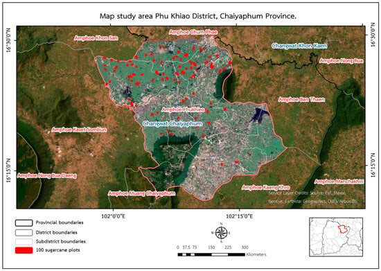
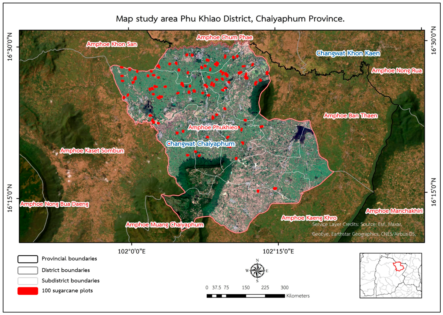
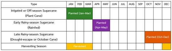
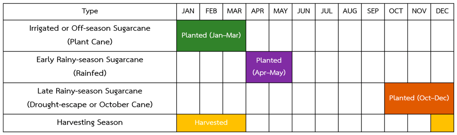
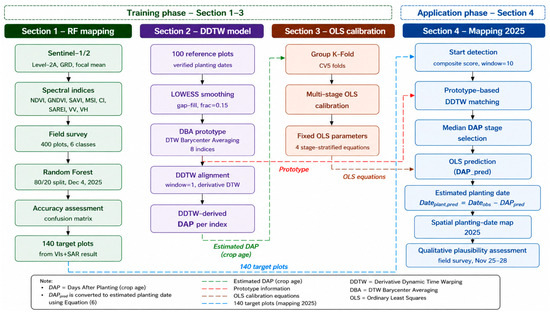
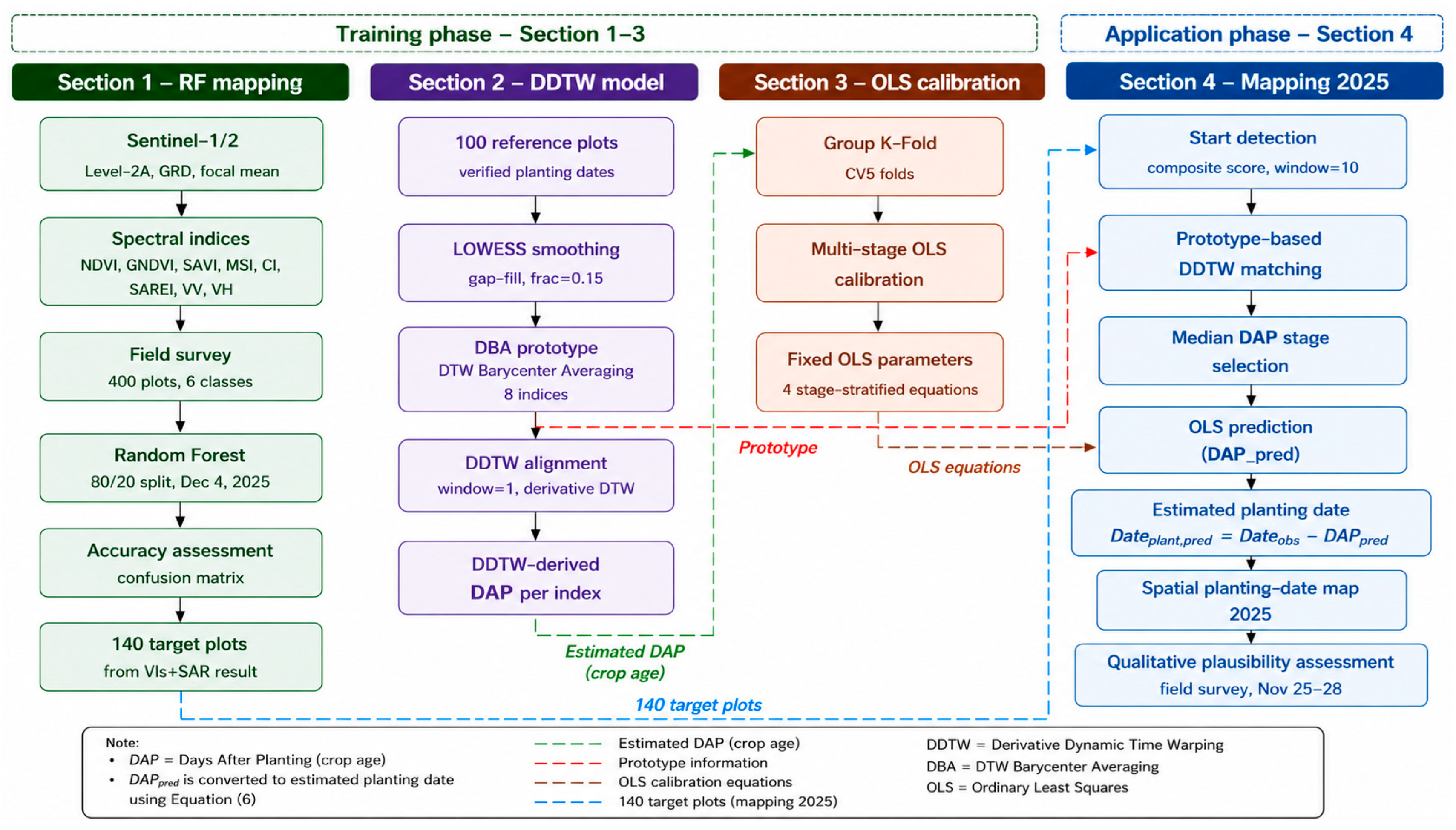
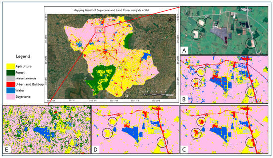
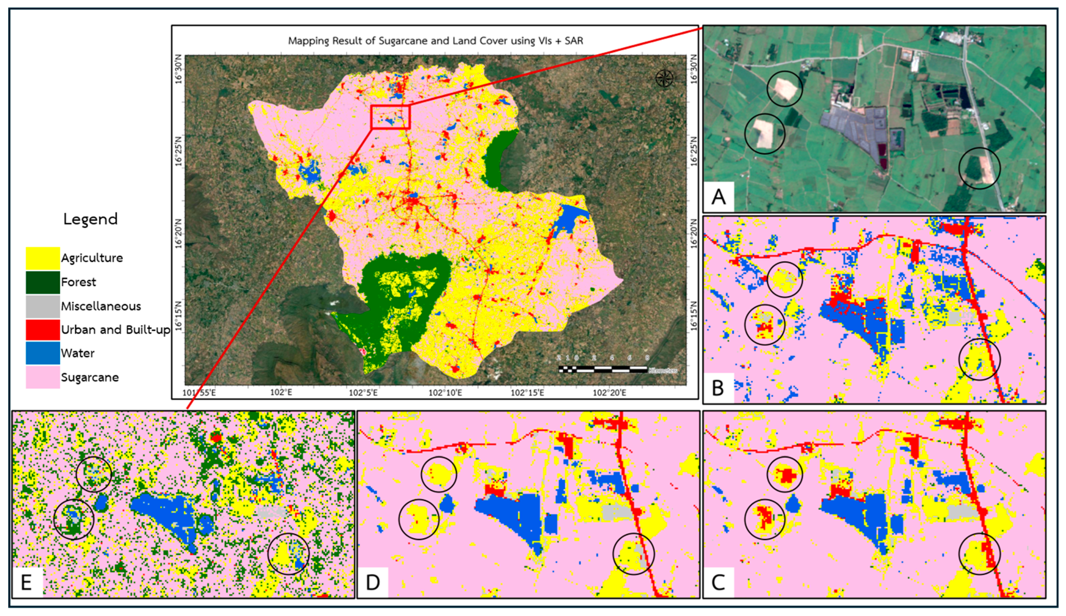
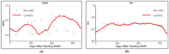
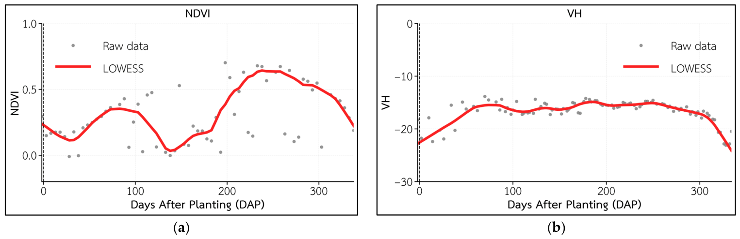
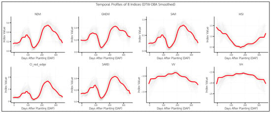
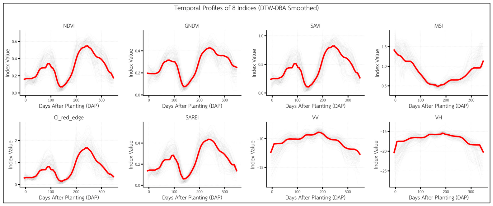
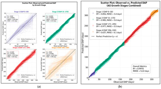
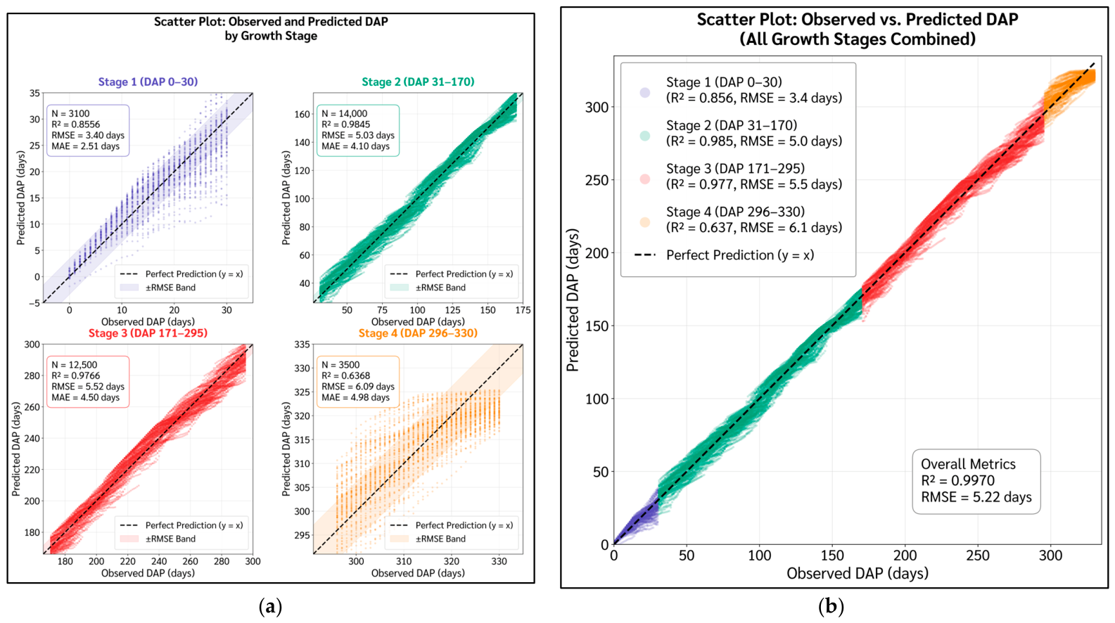
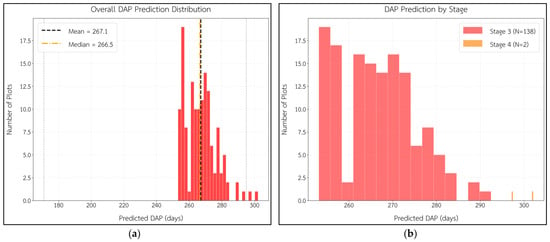
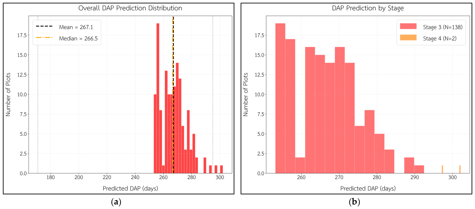
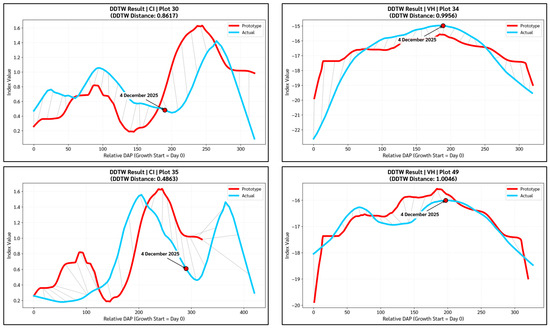
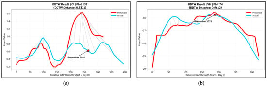
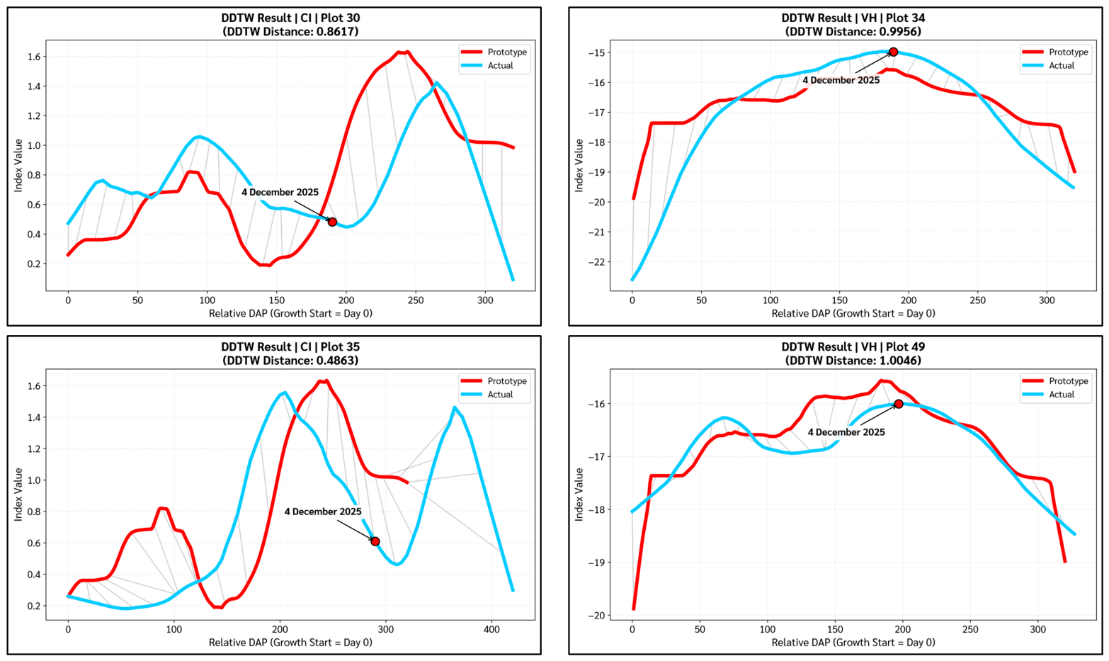
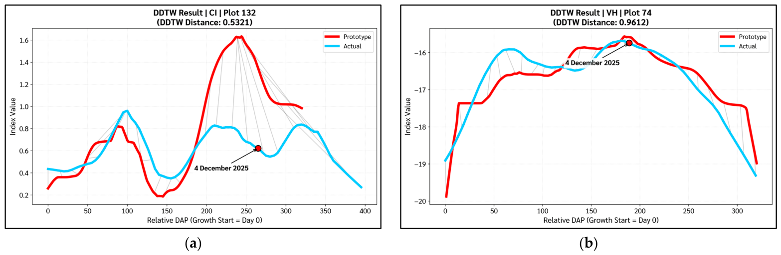
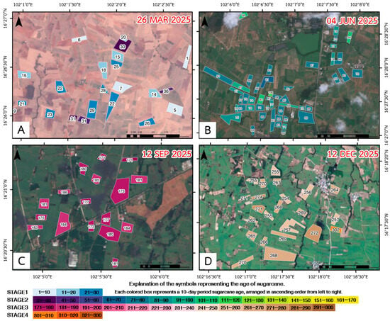
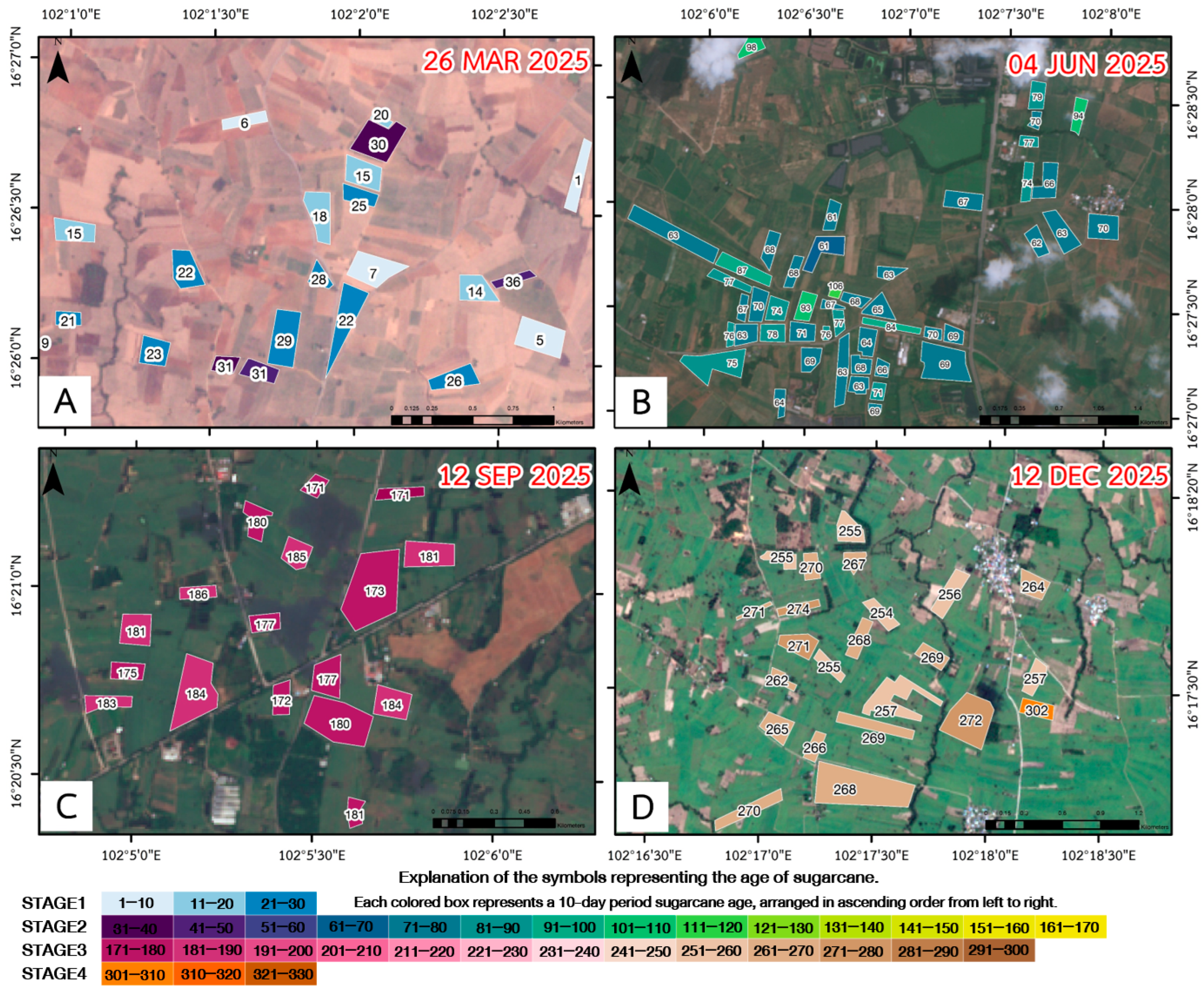
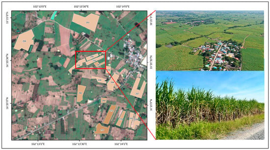
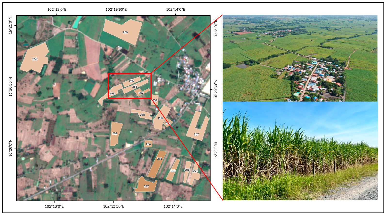

Disclaimer/Publisher’s Note: The statements, opinions and data contained in all publications are solely those of the individual author(s) and contributor(s) and not of MDPI and/or the editor(s). MDPI and/or the editor(s) disclaim responsibility for any injury to people or property resulting from any ideas, methods, instructions or products referred to in the content. |
© 2026 by the authors. Licensee MDPI, Basel, Switzerland. This article is an open access article distributed under the terms and conditions of the Creative Commons Attribution (CC BY) license.