


Abstract
Background/Objectives: Survival models can retain their ability to rank patients while their absolute-risk predictions become less accurate over time. We compared temporal calibration drift and updating across statistical and machine-learning models under competing risks. Methods: This retrospective SEER study included 881,201 women with breast cancer. Cause-specific ridge Cox, elastic-net Cox, random survival forest, and DeepSurv models were trained on diagnoses from 2004–2007 and evaluated across five two-year eras from 2008–2017. We compared fixed prediction, isotonic recalibration using the preceding two-year window, and refitting using the preceding four-year window for 5-year mortality. Results: Fixed-model breast cancer-specific mortality overprediction increased from 0.52–1.22 percentage points (pp) in 2008–2009 to 1.55–2.41 pp in 2016–2017. Discrimination remained stable or improved slightly; the latest-era inverse-probability-of-censoring-weighted area under the curve was 0.870–0.884. Latest-era residual mean calibration bias was at most 0.36 pp after isotonic recalibration and 0.57–0.97 pp after refitting. The coupled-bootstrap interval for the random survival forest bias difference included zero; refitting yielded lower Brier scores for random survival forest and DeepSurv. Calibration patterns differed by age and predicted risk. Three families first exceeded the illustrative 2-pp reference value in 2016–2017; random survival forest remained below it. Conclusions: Recalibration reduced average bias, but its advantage depended on the model and metric. Prospective evaluation must account for delayed outcome availability before these updating protocols can inform clinical practice.
1. Introduction
Prognostic survival models are essential clinical tools in oncology, guiding personalized treatment strategies such as recommending adjuvant systemic therapies following surgical resection [1,2]. However, the clinical utility of these models is inherently time-dependent [3]. Over calendar time, continuous advances in diagnostic screening, surgical techniques, therapeutic regimens, and shifts in underlying patient demographics alter population-level survival rates [4,5]. Because a model’s clinical and demographic predictor weights are typically held fixed after deployment, this mismatch leads to progressive temporal calibration drift—a silent degradation of absolute risk prediction accuracy over time [6,7]. If calibration shifts over time, a model’s absolute-risk estimates may become less accurate and could affect decisions when used to guide care [6,7].
Random survival forests (RSF) and neural survival models such as DeepSurv accommodate nonlinear predictor relationships alongside conventional Cox models [8,9,10]. Related applications of deep learning in mammographic detection and diagnosis face challenges in generalizability, interpretability, data availability, and clinical integration [11]. Survival prediction also requires explicit treatment of competing risks: death from another cause prevents a subsequent breast-cancer death, whereas right censoring leaves the subsequent outcome unknown [12]. Calibration in one cohort does not establish performance across later diagnosis eras [13]. Temporal recalibration has already been studied for survival and competing risks [14,15], as have dynamic model-maintenance pipelines [16]. We therefore examined whether calibration drift and the effects of updating differ across model families, competing outcomes, and patient subgroups.
Model complexity does not by itself establish temporal stability [17]. Updating can adjust absolute risk alone or re-estimate predictor effects from more recent patients [3,18,19,20]. Sequential Bayesian methods offer another way to update models. Tanner et al. examined dynamic updating of survival models [21], and Feng et al. developed online Bayesian logistic revision and a Markov variant with evolving revision parameters, approximating posterior updates through Kalman filtering [22]. These Bayesian, Markov, and state-space approaches overlap. Our comparison focused on post-hoc recalibration and periodic refitting; these sequential methods were not evaluated.
Using successive SEER diagnosis cohorts, we conducted a retrospective comparison of four model families for 5-year breast cancer-specific and other-cause mortality. We evaluated fixed models, specified updating protocols, and calibration within age and predicted-risk groups. The study addressed four questions:
- RQ1.
- How do the calibration and discrimination of fixed 5-year competing-risk survival models change across sequential diagnosis eras?
- RQ2.
- To what extent do the direction and magnitude of temporal calibration drift differ across model families and between breast cancer-specific and other-cause mortality?
- RQ3.
- How is temporal calibration drift distributed across age groups and predicted-risk strata, and to what extent do population-level metrics mask clinically relevant subgroup-specific patterns?
- RQ4.
- How effectively do model-agnostic isotonic recalibration and full model refitting restore temporal calibration, and how does the choice of monitoring threshold affect the timing of model updates?
2. Materials and Methods
2.1. Study Design
We conducted a retrospective simulation of temporal model maintenance using historical diagnosis cohorts with mature follow-up, including right-censored observations. Models were developed on 2004–2007 diagnoses and evaluated over the 10-year period from 2008–2017. The development and evaluation cohorts span 14 diagnosis years within the eligible 2004–2019 population. Updates used earlier diagnosis cohorts, assuming their 60-month outcomes were already available. This assumption sets aside the five-year wait for outcomes and the subsequent registry reporting delay. The comparison therefore preserves diagnosis-time separation but does not reproduce a feasible prospective update schedule.
2.2. Data Source and Study Population
Data were obtained from the National Cancer Institute’s Surveillance, Epidemiology, and End Results (SEER) 17-registry database (November 2025 submission, covering diagnoses from 2000 to 2023) under a signed data-use agreement [23]. Data were extracted using SEER*Stat software, version 9.0.43.0 (Surveillance Research Program, National Cancer Institute, Bethesda, MD, USA; https://seer.cancer.gov/seerstat/, accessed on 6 October 2026).
The final analytic study population comprised 881,201 women diagnosed with a first recorded invasive breast primary tumor between 1 January 2004, and 31 December 2019. It was derived from 886,808 candidate records after excluding 5607 records with a missing or unknown cause of death. Of these excluded records, 5538 otherwise met the eligibility criteria and 69 also failed another criterion. Inclusion was restricted to patients aged 20 years or older at diagnosis.
The temporal split was defined as follows:
- Model Development: Diagnoses from 2004–2007 (n = 196,408).
- Temporal Evaluation Eras: Five consecutive, non-overlapping two-year cohorts spanning 2008 to 2017 (total n = 558,868; ranging from 105,099 to 119,755 patients per era).
- Outside the Primary Evaluation Window: A total of 125,925 women diagnosed in 2018–2019 were retained in the eligibility definition but excluded from the primary evaluation eras because the complete tail did not have mature 60-month follow-up. The 2018–2019 cohort was examined separately for outcome availability and short-horizon sensitivity (Supplementary Table S7).
For computational efficiency, performance evaluation used a fixed-seed sample of 20,000 patients per era, shared by all four families. Post-hoc recalibrators used a separate 20,000-patient sample from the preceding two-year window; target-era outcomes were reserved for evaluation. Anchor-model development used the full 2004–2007 cohort (n =196,408), and recent refitting used all eligible patients in the preceding four-year cohorts. Only evaluation and calibrator fitting were restricted to samples; survival-model development and refitting used the full eligible cohorts.
Sample-based estimates were close to those from the full cohorts: maximum absolute differences were 0.32 pp for MCB, 0.007 for IPCW AUC, and 0.0023 for IPCW Brier score. Full-precision comparisons, including calibration-curve errors, are reported in Supplementary Table S3.
2.3. Outcome Definition
We evaluated mortality within 60 months after diagnosis using a competing-risks framework. Cause of death was determined from the SEER cause-specific and other-cause death classifications. Death attributed to breast cancer was defined as breast cancer-specific mortality (BCSM) and served as the primary event. Death from any other cause was defined as other-cause mortality (OCM) and served as the competing event. Thus, deaths from other causes were retained as competing outcomes rather than treated as loss to follow-up when estimating BCSM.
Records with a missing or unknown cause of death were excluded: 5607 in total, of whom 5538 otherwise met eligibility criteria, leaving 881,201 women in the analytic cohort. This exclusion is distinct from ordinary right censoring. Time zero () was diagnosis; follow-up ended at death, last known follow-up, or 60 months. Patients alive and event-free at 60 months were administratively censored then. The patients lost to follow-up before 60 months across the validation eras (1.8%) were censored at their last known follow-up and retained in the analysis. Observed incidence was estimated with Aalen–Johansen, and performance metrics sensitive to censoring used inverse-probability-of-censoring weights. Competing deaths remained competing outcomes.
Excluding deaths of unknown cause may introduce selection bias if missingness depends on patient characteristics or outcomes. We tested an alternative policy that assigned the 5538 otherwise-eligible deaths to OCM and repeated model development and evaluation (Supplementary Table S5). Maximum absolute differences were 0.45 pp for MCB and 0.020 for IPCW AUC. Because this policy changes both eligibility and the sampled patients, it cannot identify the true causes of death or rule out selection bias.
2.4. Predictor Definition and Preprocessing
The predictor set comprised demographic and tumor characteristics recorded during diagnostic workup and postoperative staging. We retained the original analysis’s predictor set to assess temporal drift without changing feature engineering. Follow-up began at diagnosis (), although the model uses some predictors determined after surgery. This mismatch can introduce guarantee-time bias. Without exact surgery and predictor-availability dates, we could not align follow-up to a common postoperative landmark. The model therefore does not support prediction at diagnosis.
An age-only sensitivity analysis used a predictor available at diagnosis (Supplementary Tables S4 and S5). Across all four families, BCSM MCB increased from 0.62–0.69 pp in the first era to 1.78–2.04 pp in the latest era, while BCSM AUC was 0.54–0.60 across eras. The age-only analysis checks whether the temporal pattern persists with a predictor available at diagnosis. It does not correct the timing bias in the full model or validate that model for use at diagnosis.
We harmonized staging and tumor-size variables across administrative source changes. Tumor size switched source at the 2016 boundary, so we used derived SEER recodes adjusted for comparability. Combined Summary Stage 2000 was used throughout the 2004–2017 primary period. Diagnoses from 2018 onward cross the transition to Derived Summary Stage 2018; the 2018–2019 cohort was therefore analyzed separately as a sensitivity cohort.
Unreported stage, grade, and receptor values were coded as “unknown,” indicating absent registry information rather than a clinical state. Missing tumor size and positive-node values were replaced by development-cohort medians, with a separate missingness indicator in every model family. Missingness indicators allow predictions to differ when a value is absent. They may be associated with other predictors and are not interpreted causally. Preprocessing parameters were estimated in the 2004–2007 cohort and held fixed thereafter (Table 1).
Table 1.
Predictor definitions, source variables, and preprocessing for the 2004–2017 study period. Source changes are identified where harmonization was required.
Complete-case restriction would remove 18.4–19.9% of the common evaluation samples and could alter case mix. We assessed this choice by refitting the encoder and models on complete anchor cases and evaluating complete cases within the original samples. A second variant used the full anchor cohort without missingness indicators. Because complete-case analysis changes both model fitting and the evaluated population, this comparison cannot isolate imputation bias. Median imputation may reduce variation and does not guarantee better fit or unbiased predictions. Supplementary Table S5 provides the variant-specific estimates.
Imputation replaces missing predictor values; recalibration adjusts predictions using outcomes from a later cohort. We evaluated their effects separately, without assuming either procedure was unbiased. Appendix A.3 Table A2 summarizes the preprocessing comparisons.
2.5. Model Development
We evaluated four model families, each fitted separately for BCSM and OCM using the same predictor set:
- Ridge Cox: A Cox proportional-hazards model with regularization.
- Elastic-net Cox: A Cox model combining and regularization.
- RSF: A non-parametric tree-based ensemble designed for survival outcomes [8].
- DeepSurv: A feedforward neural network trained using the Cox partial likelihood [9].
All four families used the same cause-specific fitting convention: deaths from the other cause ended follow-up without counting as target events, and right-censored patients contributed follow-up until censoring. We combined the two estimated hazards to obtain each cause’s cumulative incidence, retaining competing deaths as outcomes when estimating incidence and evaluating predictions.
The fixed hyperparameters are listed in Appendix A. To derive the cause-specific cumulative incidence function (CIF) as an absolute risk prediction under the competing-risks framework, we integrated the cause-specific hazard functions. For the ridge Cox, elastic-net Cox, and DeepSurv models, each fitted model yielded a cause-specific predictor for patient i: for the Cox models and the network output for DeepSurv.
The baseline cumulative hazard for each cause (1: BCSM; 2: OCM) was estimated by Breslow’s method in the training window, with fitted predictor effects held fixed. For patient i, the 5-year ( months) cumulative incidence was:
where is the patient’s cause-specific cumulative hazard, is the predictor row vector, and is the Cox coefficient vector. Here, is event-free survival for both causes (Appendix A, Equation (A1)). RSF supplied cause-specific cumulative hazards from its terminal nodes. All families were evaluated using the same performance metrics. BCSM risk was the cumulative incidence , rather than the complement of cause-specific survival. Implementation details are provided in File S1: Supplementary methods and detailed results.
2.6. Temporal Validation and Updating Framework
To assess stability over time, we trained the four model families on the 2004–2007 anchor window (n = 196,408) and evaluated them across five consecutive diagnosis eras from 2008–2009 to 2016–2017. Every model update used only data from years before the target evaluation era.
We applied three retrospective maintenance strategies to each model family in every era:
- Fixed prediction: The anchor model evaluated across subsequent eras without any modification to its parameters or baseline hazards.
- Isotonic recalibration: A non-parametric mapping adjusted fixed-model predictions using censoring-weighted 60-month outcomes from the preceding two-year window. The mapping was then applied to the target era. Each cause was recalibrated separately, without imposing a joint probability constraint. An auxiliary rescaling analysis checked predictions whose two cause-specific risks summed above one (Supplementary Table S10); this correction was not part of the primary protocol or its bootstrap.
- Recent refitting: A complete retraining of the model family’s parameters (re-estimating coefficients, network weights, and baseline hazards) using the full cohort from the preceding four-year sliding window (e.g., refitting on 2012–2015 data to predict outcomes in the 2016–2017 era).
Sensitivity analyses varied the recalibration window (1–5 years), recalibration method (isotonic, logistic, or weighted LOESS), hyperparameters, missing-data handling, and evaluation sampling. Nominal windows were truncated at 2004 in the earliest era. The method comparison used identical preceding two-year samples and IPCW weights, with evaluation in the target era (Supplementary Table S6). Smoother settings are given in the Supplementary Methods. Fitting a calibrator to target-era outcomes would remove this temporal separation and assess contemporaneous calibration instead.
We performed several sensitivity analyses. First, for ridge Cox, elastic-net Cox, and DeepSurv, we updated only the baseline hazard while keeping the fitted coefficients or neural-network weights unchanged. This tested whether calibration drift mainly reflected a change in the underlying event rate. This analysis was not applicable to RSF because it does not have a separate baseline-hazard component.
We evaluated frozen predictions at 12, 24, 36, and 60 months, including whether one era’s 12-month calibration bias was associated with the next era’s 60-month bias. Additional analyses examined short-horizon recalibration, transfer of a 12-month calibrator to five-year predictions, annual diagnosis cohorts, and outcome availability in 2018–2019 (Supplementary Tables S1 and S7).
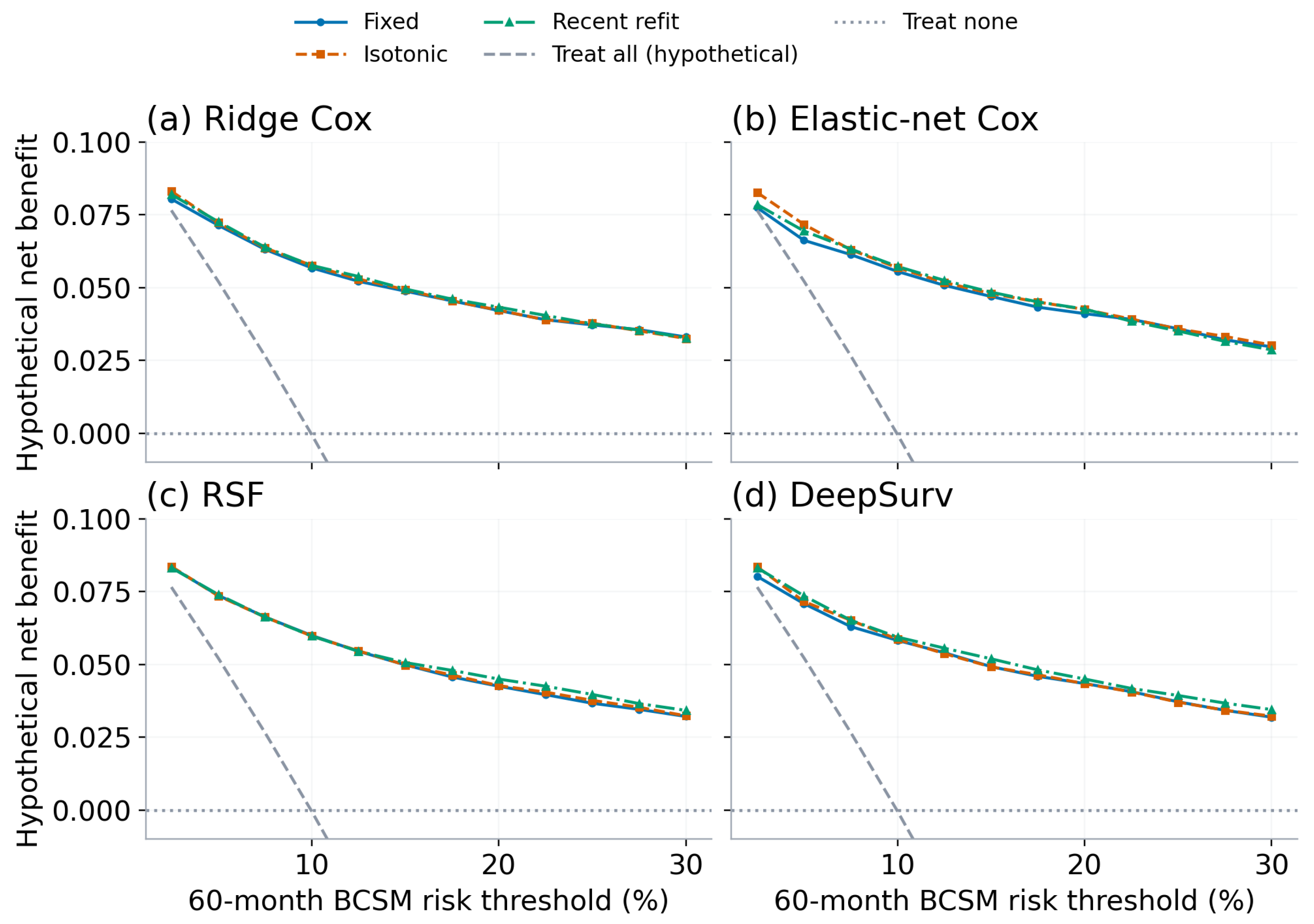
Exploratory decision-curve analysis used hypothetical cause-specific five-year risk thresholds of 2.5–30%, with treat-all and treat-none references [24,25]. The thresholds were exploratory and were not based on a treatment guideline or validated action cutoff. Net benefit weighted false positives according to the selected threshold; competing deaths counted as non-cases and IPCW accounted for right censoring. The weighting rule is specified in the Supplementary Methods. With no specified intervention or treatment effect, these decision curves describe a hypothetical decision rule and cannot establish clinical benefit.
2.7. Model Performance and Calibration Metrics
All metrics were evaluated at 60 months. We estimated observed cumulative incidence with the Aalen–Johansen estimator; IPCW metrics accounted for right censoring, while deaths from competing causes remained competing events [12]. We estimated censoring weights within each sample using a marginal reverse Kaplan–Meier estimator, assuming censoring was independent of event time and cause and that censoring-survival probabilities remained positive. Weight calculation and numerical safeguards are described in the Supplementary Methods.
The primary calibration metric was the Mean Calibration Bias (), expressed in percentage points (), which represents the average predicted absolute risk minus the observed Aalen–Johansen cumulative incidence:
where N is the number of patients in the evaluation cohort, is the predicted CIF at months and is the cohort’s Aalen–Johansen estimate. Positive MCB indicates overprediction; negative MCB indicates underprediction. MCB expresses the average discrepancy in absolute risk, but a value near zero can conceal errors within patient or risk groups. It differs from the regression-derived calibration intercept with slope fixed at one. We therefore also assessed calibration curves, ICI, , and calibration intercept and slope.
Multiplication by 100 converts the difference between the two CIF fractions to percentage points. We estimated calibration intercept and slope by IPCW-weighted logistic regression of the cause-specific outcome on predicted-risk logits; calibration-in-the-large fixed the slope at one. ICI and summarize mean and maximum deviations of a weighted LOESS calibration curve on the risk-fraction scale. Numerical safeguards are specified in the Supplementary Methods.
Secondary metrics were ICI and for calibration, cumulative/dynamic IPCW AUC for discrimination, and IPCW Brier score for overall prediction error [26,27,28,29,30]. For cause-specific AUC, cases were target-cause deaths by 60 months; controls included patients without a target-cause death, including those who died from the competing cause. The Brier score used the same binary outcome definition. IPCW accounted for right censoring in both metrics.
Evaluation uncertainty. Primary MCB and IPCW Brier-score intervals used 500 evaluation-bootstrap replicates; additional metric and calibration-curve intervals used 200. Patients were resampled with replacement, and censoring weights and performance measures were recalculated while fitted models and calibrators remained fixed. Calibration-curve intervals were pointwise, not simultaneous. Paired strategy comparisons used 500 shared patient resamples, with original-sample differences as point estimates (Supplementary Tables S1 and S2).
Update-estimation uncertainty. A complementary 200-replicate bootstrap re-estimated updates in the latest era. Resampling preserved the shared patients between recalibration and refitting; evaluation patients were resampled independently, using the same draw for both strategies. Both cause-specific refit models and calibrators were re-estimated, and predictions, censoring weights, and metrics were recalculated. The anchor model, encoder, selected samples, hyperparameters, and fitting seeds remained fixed (Supplementary Table S2).
We used 95% percentile intervals and reported original-sample estimates separately from bootstrap means. The resampling algorithm and random seeds are given in the Supplementary Methods. Initial anchor-development uncertainty was not propagated. Recalibration used two years and 20,000 patients, whereas refitting used four years and all eligible patients. Their comparison therefore reflects both the updating method and the available update data.
We described calibration by age group and predicted-risk decile in the full evaluation cohorts. Risk deciles were defined separately within each family and era; observed incidence was estimated within each subgroup (Supplementary Table S8). We recorded the first era to cross each illustrative MCB cutoff without prespecifying a clinical action threshold.
3. Results
3.1. Study Cohort and Temporal Eras
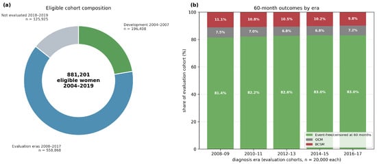
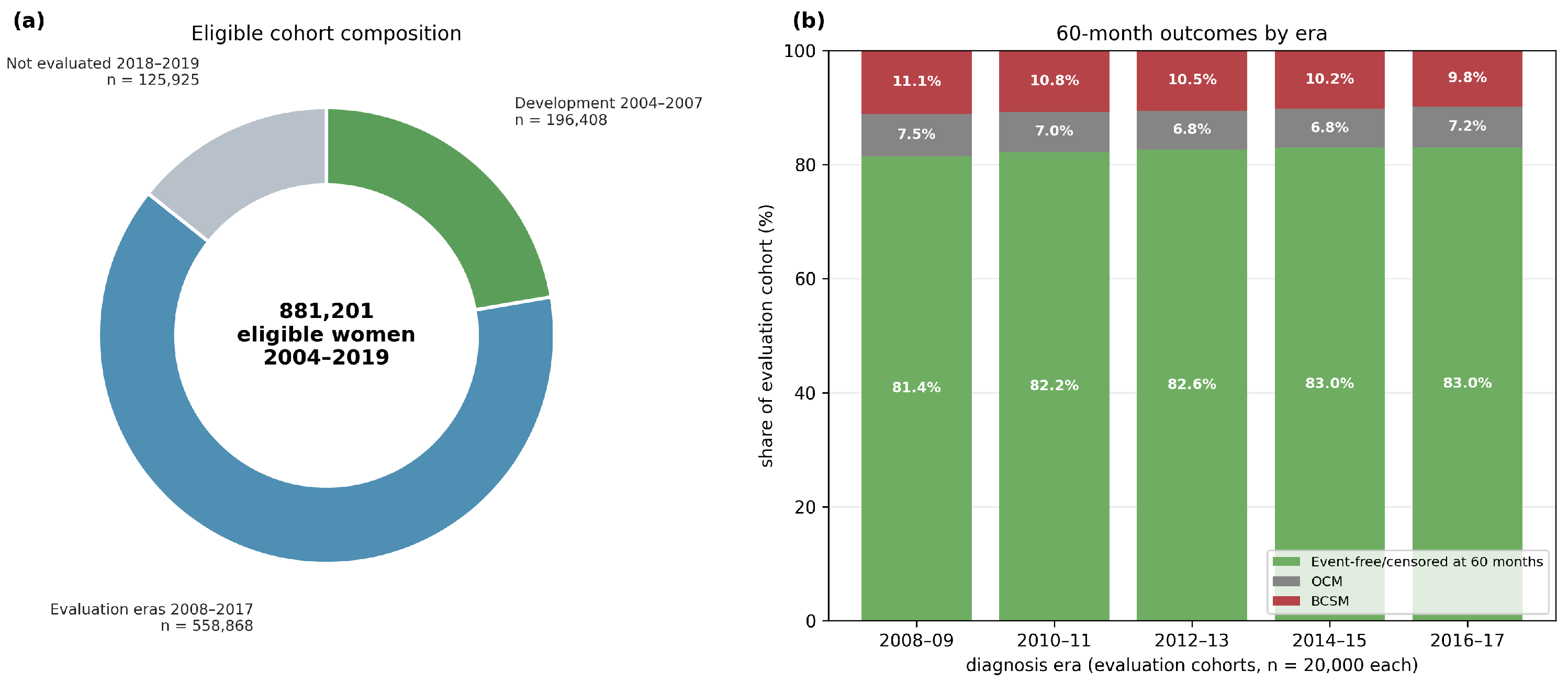
The analysis included 196,408 women in the 2004–2007 development cohort and 558,868 women across five evaluation eras from 2008 to 2017 (Figure 1a). The common evaluation samples comprised 20,000 patients per era (100,000 in total). Across these samples, the number of 60-month breast cancer-specific mortality (BCSM) events decreased from 2227 to 1962, whereas other-cause mortality (OCM) events remained comparatively stable (Figure 1b).
Figure 1.
Cohort composition and calendar-time validation design. (a) The eligible population of 881,201 women was divided into the development window (2004–2007), five evaluation eras (2008–2017), and the 2018–2019 period outside the primary analysis. (b) Each reproducible 20,000-patient evaluation sample was classified by 60-month outcome; BCSM decreased across eras while OCM remained comparatively stable. Percentages in panel (b) are based on these evaluation samples and may therefore differ slightly from the full-cohort estimates in Table 2.
Table 2 summarizes the cohort characteristics. Median age and tumor size remained stable. The proportion of localized disease increased from 61.3% to 64.6%, while estrogen-receptor positivity increased and unknown receptor status became less common.
Table 2.
Clinical and tumor characteristics of the full development cohort (2004–2007) and the five temporal evaluation cohorts (2008–2017).
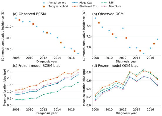
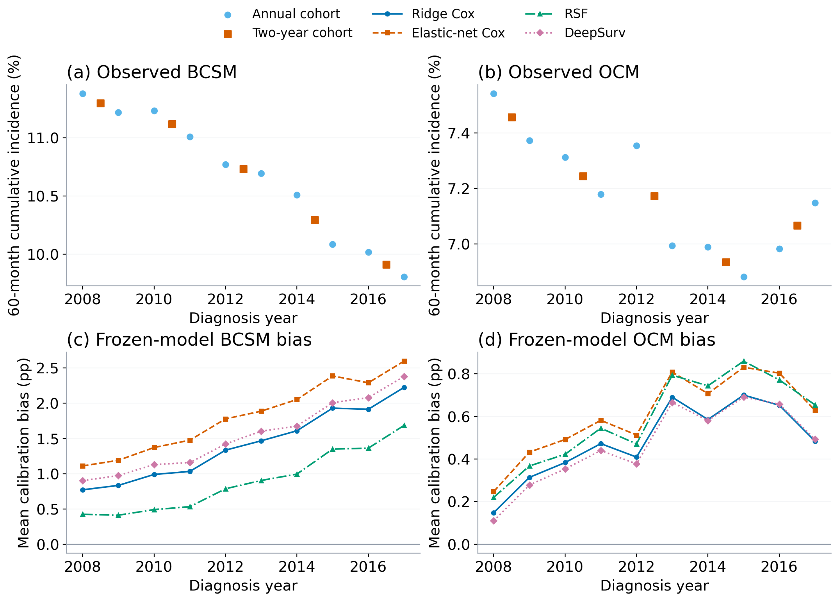
In the full two-year cohorts, observed BCSM decreased from 11.30% in 2008–2009 to 9.91% in 2016–2017; OCM remained between 6.9% and 7.5%. Annual full-cohort BCSM was 11.38% in 2008 and 9.81% in 2017, with variation between years. Figure 2 shows annual incidence and frozen-model MCB for distinct diagnosis cohorts. The series compares different patients across diagnosis years. The separate 2018–2019 cohort was evaluated at 12, 24, and 36 months (Supplementary Table S7); Section 3.6 reports its five-year outcome availability.
Figure 2.
Full-cohort observed 60-month cause-specific cumulative incidence and frozen-model MCB by diagnosis year, 2008–2017. Each point represents a distinct cohort; connecting lines show calendar-time ordering only.
3.2. Discrimination of Fixed Models
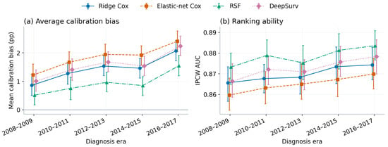
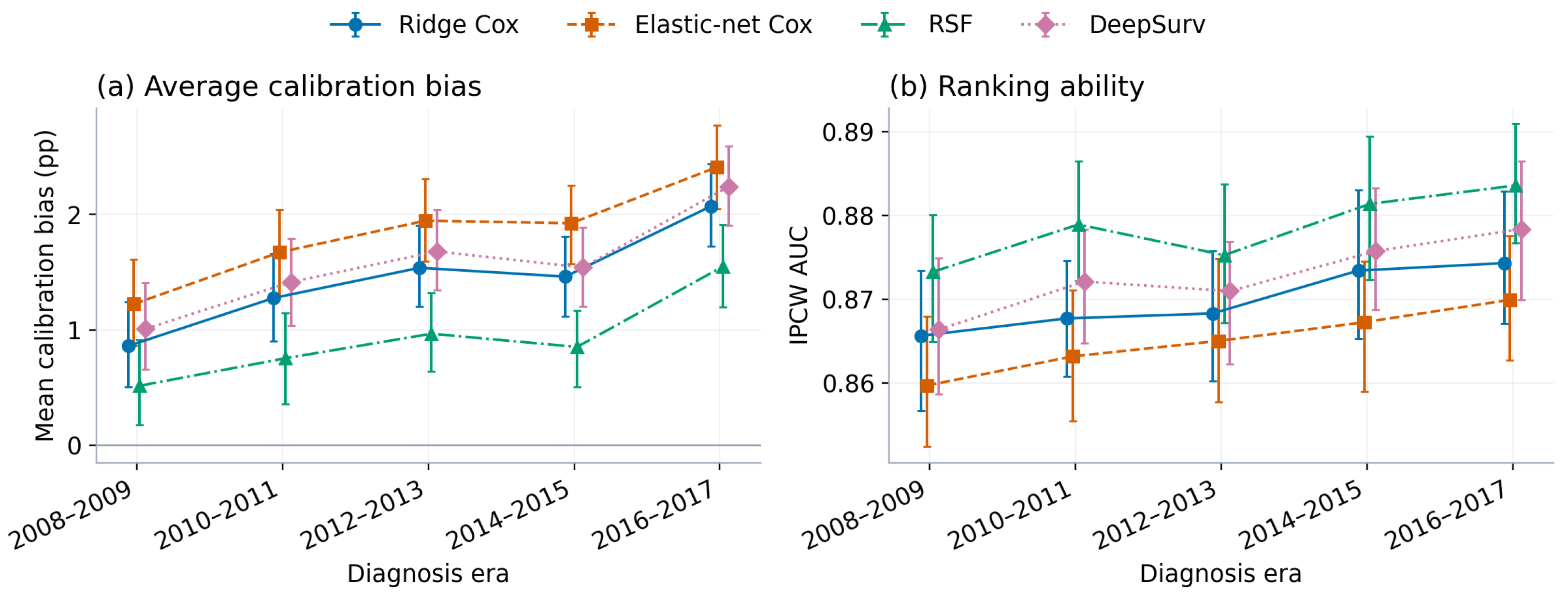
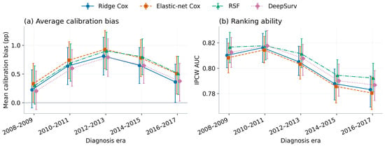
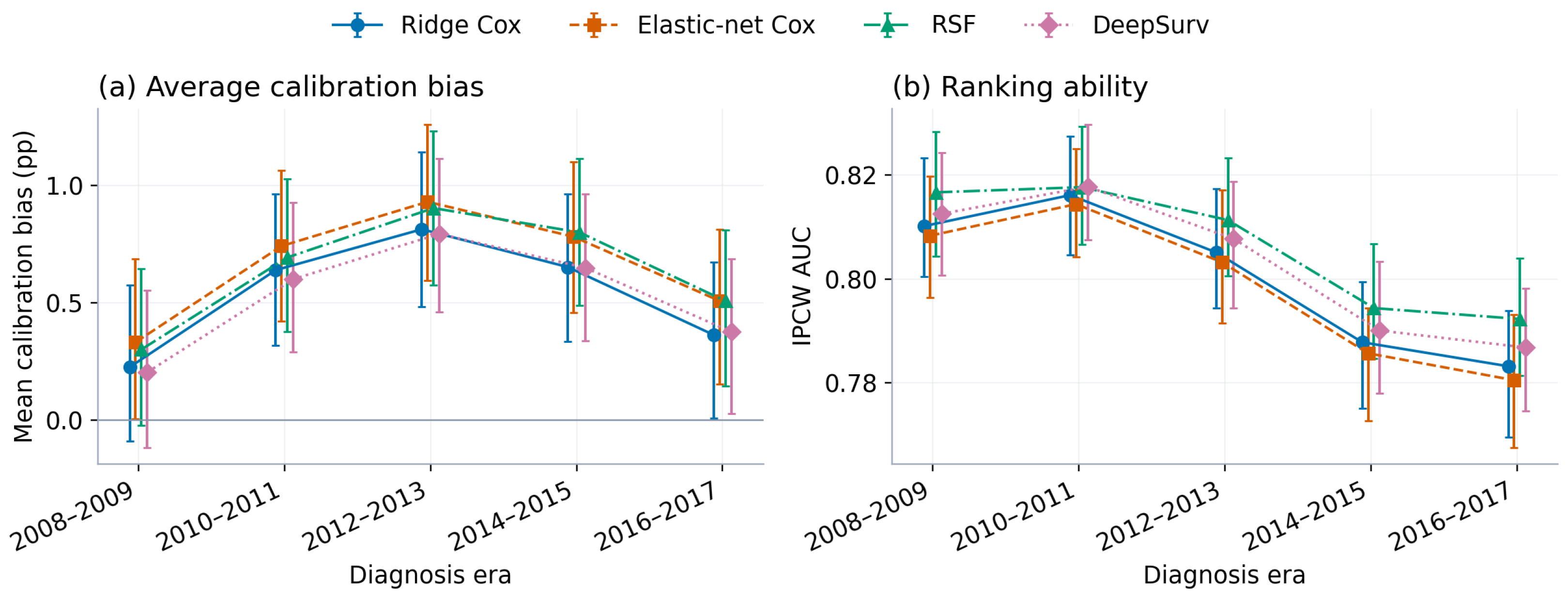
Discrimination remained stable or improved slightly over time (Figure 3b). Across the four families, IPCW AUC ranged from 0.860 to 0.873 in 2008–2009 and from 0.870 to 0.884 in 2016–2017. RSF had the highest AUC throughout the study.
Figure 3.
Fixed-model performance for breast cancer-specific mortality (BCSM): (a) mean calibration bias (MCB) with 95% bootstrap confidence intervals; (b) IPCW area under the receiver operating characteristic curve (AUC) with 95% percentile intervals from 200 evaluation-bootstrap replicates. MCB intervals use 500 replicates. All intervals are conditional on frozen fits. Positive MCB indicates overprediction. Eras are distinct cohorts; connecting estimates indicates calendar-time ordering only.
3.3. Temporal Calibration Drift
BCSM calibration bias was higher in the last evaluation era than in the first for all four fixed model families, despite stable or slightly improved discrimination (Table 3; Figure 3a).
3.3.1. Breast Cancer-Specific Mortality
Observed BCSM declined while fixed models continued to predict risks closer to those of earlier cohorts. Full-cohort MCB slopes were 0.14–0.17 pp per year. Across model families, MCB increased from 0.52–1.22 pp in the first era to 1.55–2.41 pp in the latest era (Table 3), with the smallest bias for RSF and largest for elastic-net Cox. Latest-era observed-to-expected ratios were 0.81–0.87. Full-cohort checks confirmed the BCSM drift pattern (Supplementary Tables S1 and S3).
Table 3.
Frozen-model BCSM mean calibration bias across diagnosis eras. MCB is expressed in pp; IPCW AUC is shown for 2016–2017.
3.3.2. Calibration by Age
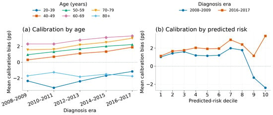
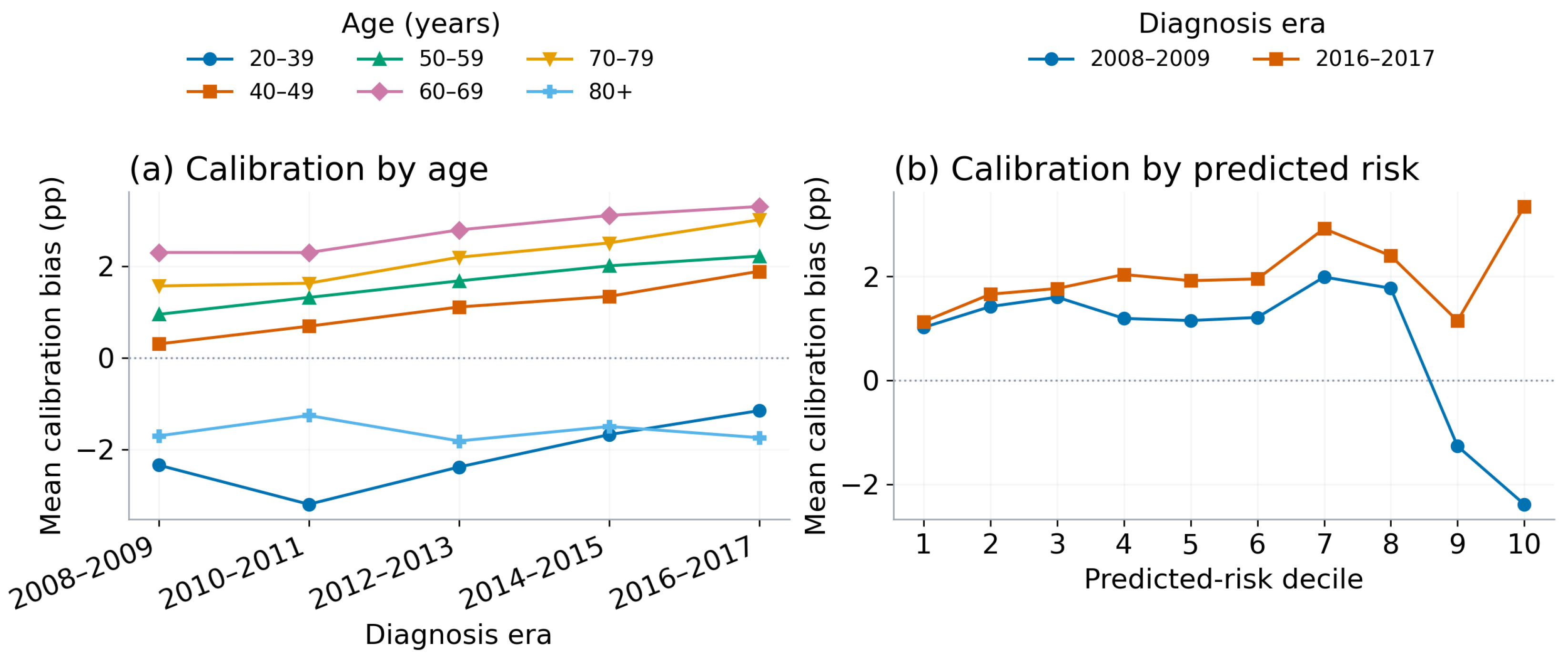
Calibration patterns differed by age (Figure 4a). For fixed ridge Cox, MCB increased most at ages 40–49 (from 0.30 to 1.89 pp) and 70–79 (from 1.57 to 3.01 pp) between the first and latest eras. The youngest group remained underpredicted (from to pp), as did the 80+ group (from to pp). In the latest era, MCB reached 3.30 pp at ages 60–69. Full-cohort age-specific estimates for all families are reported in Supplementary Table S8. These subgroup comparisons are descriptive.
Figure 4.
Subgroup MCB for the fixed ridge Cox model in distinct evaluation cohorts: (a) by age group across eras and (b) by predicted-risk decile in the first and latest eras. Positive and negative values indicate over- and underprediction, respectively. Results for all four families are shown in Appendix A.5 Figure A2 and Figure A3. Each era represents a different cohort, not repeated measures on the same patients.
3.3.3. Calibration by Risk Group
Average MCB also masked differences across predicted-risk deciles (Figure 4b). For ridge Cox in 2008–2009, the three lowest-risk deciles were overpredicted by 1.0–1.6 pp, while the highest-risk decile was underpredicted by 2.4 pp. This pattern weakened over time. By 2016–2017, every decile was overpredicted, including the highest-risk decile by 3.3 pp (Supplementary Table S8).
3.3.4. Other-Cause Mortality
OCM calibration errors remained below 0.93 pp for all families and eras (Figure 5a). OCM discrimination was lower than for BCSM, with IPCW AUC values of 0.78–0.82 (Figure 5b). Supplementary Table S1 gives the calibration-curve metrics, and the Supplementary Methods describe the numerical integration check.
Figure 5.
Fixed-model performance for other-cause mortality (OCM): (a) MCB with 95% bootstrap confidence intervals; (b) IPCW AUC with 95% percentile intervals from 200 evaluation-bootstrap replicates. MCB intervals use 500 replicates. All intervals are conditional on frozen fits. Positive MCB indicates overprediction. Eras are distinct cohorts; connecting estimates indicates calendar-time ordering only.
3.4. Model Updating
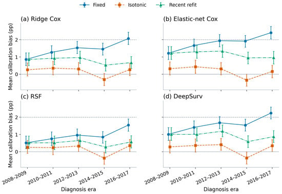
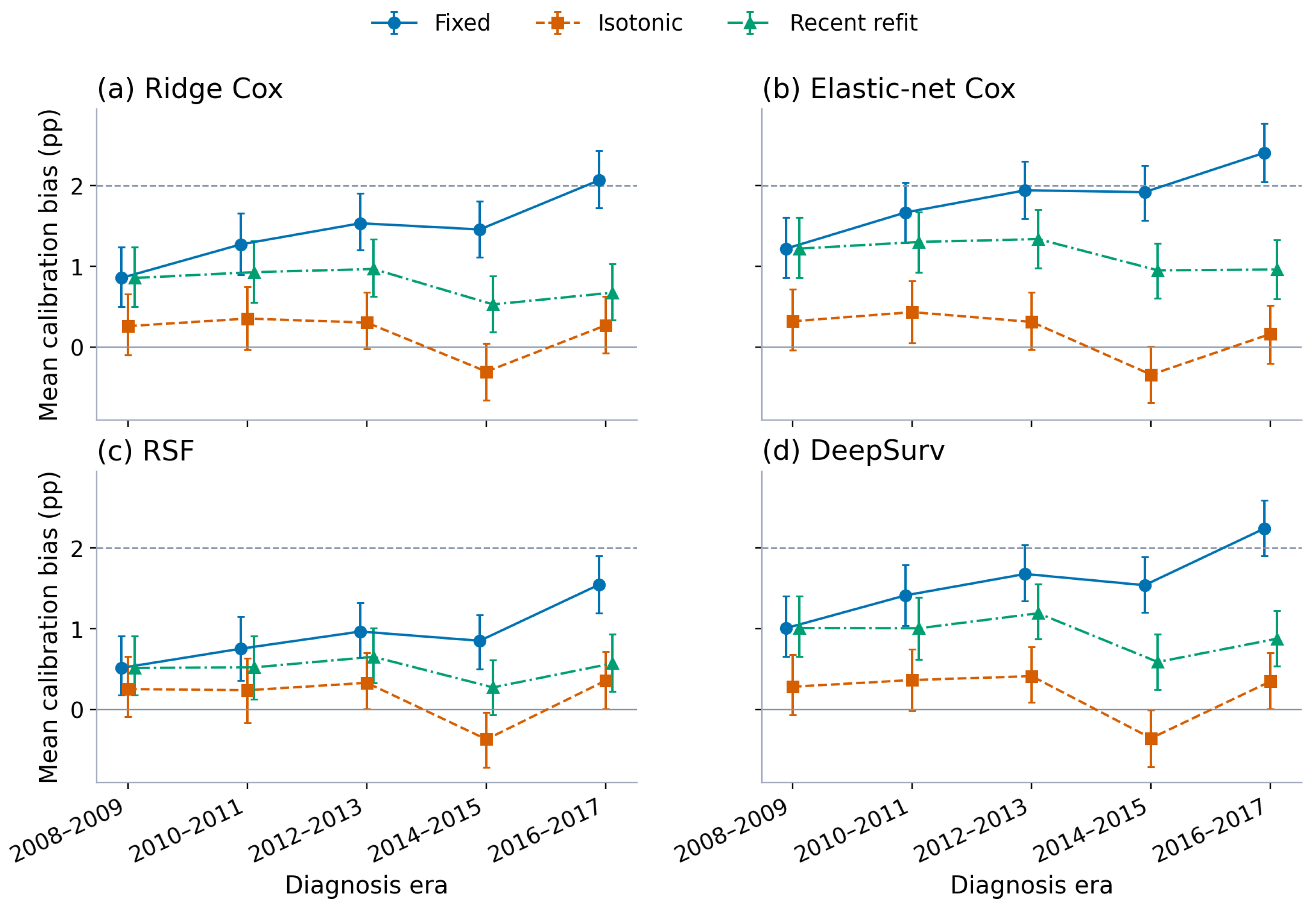
Table 4 compares the three strategies in the latest era; Figure 6 shows how their calibration bias changed across eras.
Table 4.
BCSM calibration bias and discrimination by updating strategy in 2016–2017. Values are MCB in pp [95% CI], with IPCW AUC in parentheses. Intervals are conditional on fitted models and updates.
Figure 6.
Breast cancer-specific mortality (BCSM) mean calibration bias by strategy and diagnosis era for (a) ridge Cox, (b) elastic-net Cox, (c) RSF, and (d) DeepSurv. Error bars show 95% percentile intervals from 500 evaluation-bootstrap replicates, conditional on fitted models and updates. The dashed horizontal line marks the illustrative 2-percentage-point monitoring threshold. Each era is a distinct diagnosis cohort; connecting estimates indicates calendar-time ordering only.
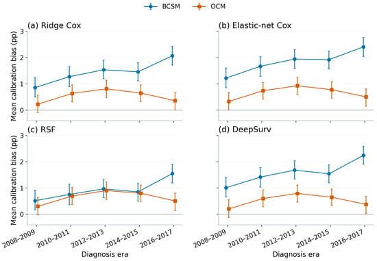
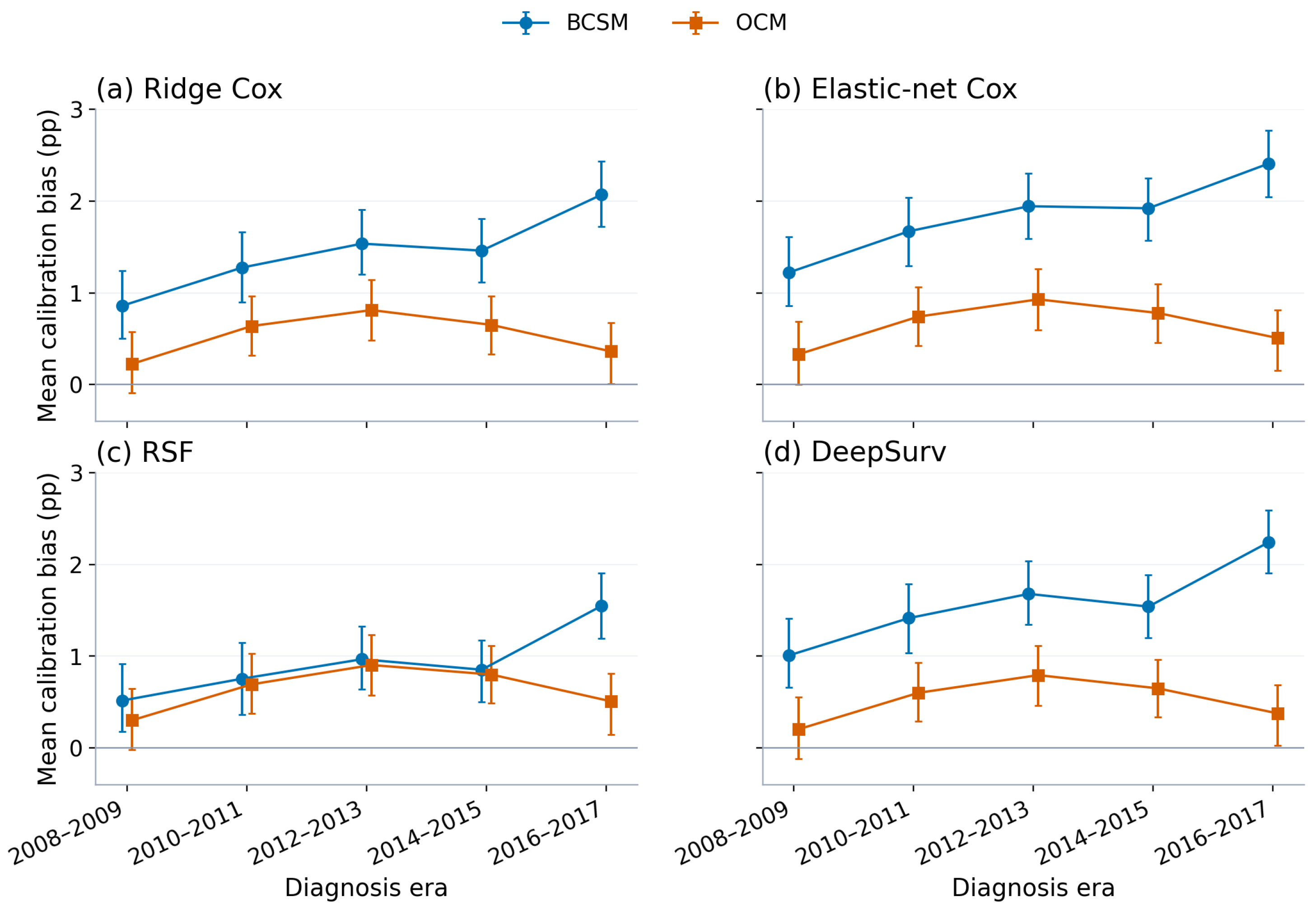
Figure 7 displays signed MCB for both causes by model family; positive and negative values indicate over- and underprediction, respectively.
Figure 7.
Signed frozen-model mean calibration bias (MCB) for BCSM and OCM across evaluation eras, shown in a separate panel for each model family. Positive values indicate overprediction and negative values indicate underprediction. All panels use the same vertical scale and show 95% evaluation-bootstrap intervals conditional on the frozen models. Each era is a distinct diagnosis cohort; connecting lines indicate calendar-time ordering only.
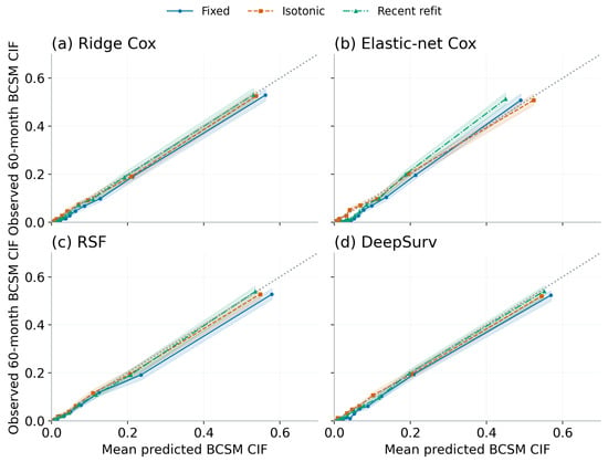
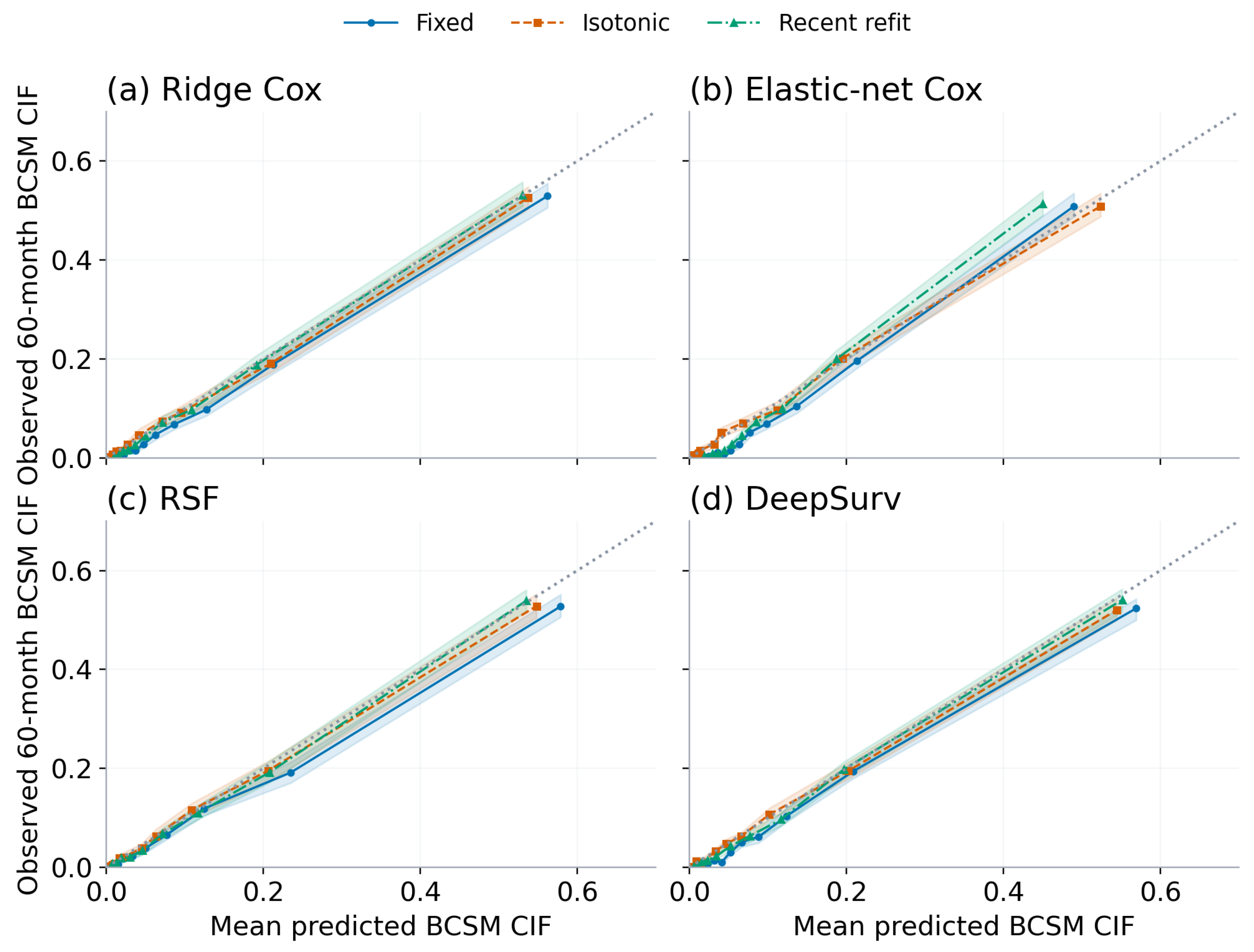
Isotonic recalibration reduced BCSM bias to 0.17–0.36 pp across all families and changed AUC by no more than 0.001 (Figure 8). For RSF, it also reduced OCM bias from as much as 0.90 pp to no more than 0.53 pp.
Figure 8.
BCSM calibration curves (predicted versus observed binned incidence) in 2016–2017 for (a) ridge Cox, (b) elastic-net Cox, (c) RSF, and (d) DeepSurv. Curves compare fixed prediction, isotonic recalibration, and recent refitting; the dotted line is the identity. Shading shows pointwise binwise 95% percentile intervals from 200 evaluation-bootstrap replicates, conditional on fitted models and updates. Prediction-quantile bins were re-formed in each replicate; the shading is not a simultaneous confidence band.
Supplementary Figure S1 presents calibration curves for all four model families, all five evaluation eras, both causes, and all three primary strategies.
Updating only the baseline hazard removed 65–74% of the original bias, leaving late-era MCB of 0.54–0.79 pp in the Cox-based families, with little change in discrimination. This update is not defined for RSF. Family-specific estimates are reported in Supplementary Table S4.
Recent refitting left latest-era residual BCSM MCB of 0.57–0.97 pp, compared with at most 0.36 pp after isotonic recalibration. Refitting increased IPCW AUC by approximately 0.002–0.006 over the frozen models. Lower average signed bias does not establish better calibration at every risk level or lower overall prediction error.
Some frozen and isotonic-recalibrated AUC values coincide after rounding to three decimals. Strictly increasing mappings preserve ranking, but isotonic plateaus introduce ties that can change AUC. For latest-era RSF, the values round to 0.884 before and 0.883 after recalibration. The small AUC changes can vary across eras as risk distributions and ties change.
Latest-era original-sample isotonic-minus-refit BCSM MCB differences ranged from approximately to pp across families. Paired evaluation-bootstrap intervals excluded zero when the fitted updates were held fixed. They do not include update-estimation uncertainty and compare signed bias rather than absolute calibration error. Supplementary Table S2 reports all 40 family-era-cause contrasts for MCB, AUC, and Brier score, with pointwise intervals and no multiplicity adjustment.
Re-estimating updates in the coupled bootstrap widened the uncertainty intervals. The RSF BCSM MCB-difference interval included zero (approximately to 0.09 pp), as did its AUC-difference interval. Brier-score difference intervals favored refitting for RSF and DeepSurv; all four OCM MCB-difference intervals included zero. Table 5 summarizes the latest-era BCSM contrasts; Supplementary Table S2 gives the full family-specific intervals, original-sample contrasts, and bootstrap means. These intervals remain conditional on the anchor model, encoder, selected samples, hyperparameters, and fitting seeds.
Table 5.
Paired comparison of isotonic recalibration and recent refitting for BCSM in 2016–2017. Values are original-sample differences [95% percentile intervals] from 200 coupled update-bootstrap replicates. Full results are in Supplementary Table S2.
Isotonic recalibration reduced the observed ranges of BCSM Brier score, ICI, and across families and eras. Because these ranges span different cohorts, their reduction does not quantify paired improvements. In the latest era, refitting yielded lower Brier scores than isotonic recalibration for RSF and DeepSurv, and lower for RSF. Thus lower average bias did not imply better performance on every metric. Supplementary Table S1 reports all five metrics, calibration parameters, and conditional intervals for each family, era, cause, and primary strategy.
3.5. Sensitivity Analyses
With identical preceding two-year data, LOESS and isotonic recalibration differed by at most 0.32 pp in MCB across families, eras, and causes (mean absolute difference 0.09 pp); the maximum logistic-versus-isotonic difference was 0.14 pp. Supplementary Figure S2 shows these comparisons. Table 6 summarizes the latest-era BCSM mean calibration bias for one-, two-, and three-year recalibration windows and for logistic recalibration using a two-year window.
Table 6.
Sensitivity of BCSM mean calibration bias to preceding window length and recalibration method in 2016–2017. Values are MCB in pp [95% CI] from 500 paired evaluation-bootstrap replicates, conditional on fitted models and calibrators. Full results are in Supplementary Table S6.
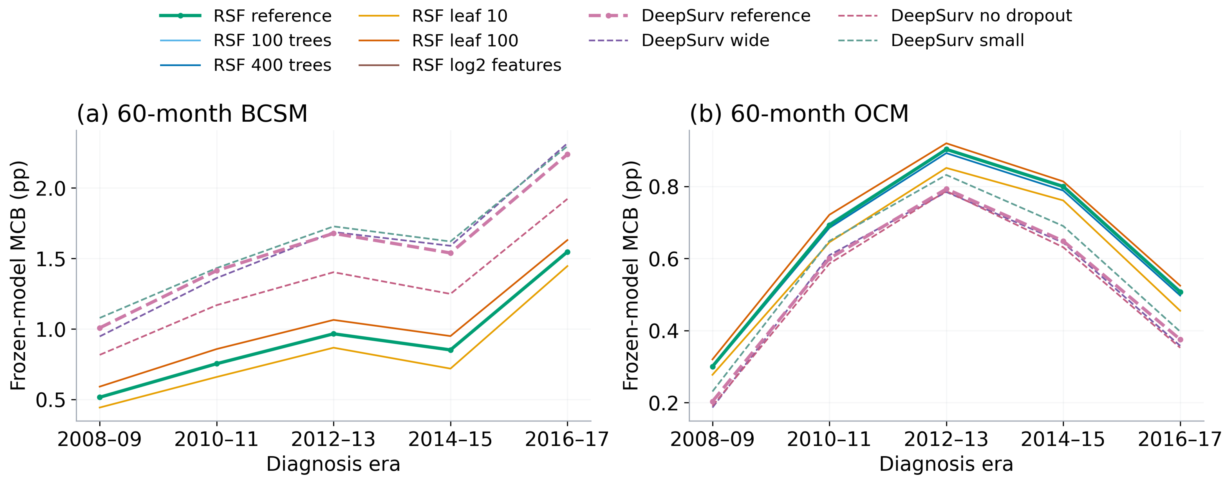
Across six RSF and four DeepSurv configurations, including one reference per family and eight alternatives, all BCSM drift slopes remained positive. Latest-era MCB was 1.45–1.63 pp for RSF and 1.92–2.32 pp for DeepSurv (Appendix A.2 Table A1 and Figure A1). Supplementary Table S4 provides the configurations and full era-specific estimates. The drift pattern persisted across the tested settings; other configurations may behave differently.
Complete-case refitting changed MCB by at most 0.98 pp and IPCW AUC by 0.053. Removing missingness indicators changed MCB by at most 0.50 pp (Appendix A.3 Table A2; Supplementary Table S5). Complete-case comparisons change the evaluated population as well as model fitting and cannot isolate imputation bias. Calibrators always used preceding-window outcomes, preserving the specified separation from the target era.
Separate cause-wise isotonic mappings produced risk sums above one in at most 0.47% of patients; frozen and recently refitted predictions did not exceed one. Auxiliary proportional rescaling changed MCB by at most 0.011 pp, with small changes in AUC and Brier score. However, changed by as much as 0.097 on the risk-fraction scale, showing sensitivity of tail calibration to this correction (Supplementary Table S10).
3.6. Monitoring Thresholds
We evaluated 2 pp as a readily interpretable reference discrepancy, alongside 1.5- and 2.5-pp cutoffs. Ridge Cox, elastic-net Cox, and DeepSurv first exceeded it in 2016–2017; RSF did not (Appendix A.4 Table A4). Recalibration reduced MCB below 0.4 pp. Appendix A.4 Table A3 reports cutoff sensitivity. The cutoffs illustrate monitoring sensitivity and are not clinical action thresholds.
At 1.5 pp, elastic-net Cox first crossed the reference value in 2010–2011, ridge Cox and DeepSurv in 2012–2013, and RSF in 2016–2017. No family crossed 2.5 pp. Thus, the selected cutoff changes the first crossing era without establishing when a clinical model should be updated. An operational trigger would require validation against baseline risk and the consequences of unnecessary or delayed updates.
Across four successive era pairs per family, correlations between 12-month BCSM bias and next-era five-year bias ranged from to 0.07. Recalibration at the same short horizon left MCB between and 0.38 pp. Transferring a 12-month calibrator to five-year predictions produced underprediction of 2.62–3.88 pp. Neither the lead–lag correlations nor calibrator transfer supported prospective drift prediction or reliable transfer between horizons.
Calibration bias at shorter horizons was associated with five-year bias within the same cohorts. Earlier outcomes were also more complete: in 2018–2019, status was known for approximately 97–99% of patients at 12–36 months, compared with 50.9% at five years. Earlier outcomes may provide faster feedback, but their association with five-year bias in the same cohort does not establish a surrogate for mature five-year calibration. Supplementary Table S7 provides the associations, recalibration results, and outcome-availability estimates.
3.7. Decision-Curve Analysis
For the hypothetical BCSM decision rule at a 10% threshold, frozen-model net benefit declined by 11.1–13.5% relative to the first era. Changes after recalibration varied with model family and threshold (Appendix Figure A4; Supplementary Table S9). These changes describe the hypothetical trade-off between false positives and true positives; they do not demonstrate treatment benefit.
4. Discussion
4.1. Principal Findings
Calibration deteriorated across statistical, forest, and neural survival models even when discrimination remained stable. Fixed-model BCSM overprediction increased as observed 5-year BCSM declined. A stable AUC therefore masked worsening absolute-risk predictions.
The cohort average also concealed different patterns within patient groups. For ridge Cox, the youngest and oldest groups remained underpredicted, whereas RSF overpredicted risk in the youngest group. Ridge Cox changed from overprediction in lower-risk deciles and underprediction at the highest risks to overprediction across all deciles. Subgroup calibration therefore depended on the model family and was not captured by overall MCB alone.
Isotonic recalibration had lower latest-era BCSM MCB point estimates than refitting in every family, with small AUC changes. That result is specific to average bias: the coupled RSF MCB-difference interval included zero, while refitting yielded lower Brier scores for RSF and DeepSurv and lower for RSF. Baseline-hazard updating also reduced bias in the Cox-based models. The preferred update therefore depended on the performance metric. The short-horizon analyses also provided no established advance warning of later drift.
4.2. Implications for Model Monitoring and Maintenance
Monitoring absolute-risk predictions requires calibration measures alongside AUC. A model can retain useful ranking while its predicted mortality becomes increasingly pessimistic. Tracking average bias together with calibration curves distinguishes changes in population risk from errors concentrated at particular risk levels.
Population averages may also hide errors within age or risk groups. Monitoring by clinically relevant subgroups may identify patterns that are missed by overall MCB. The different behavior of BCSM and OCM further supports evaluating each competing outcome separately.
Recalibration may be a practical update when discrimination remains stable because it adjusts absolute risk without replacing the full model. Its feasibility depends on having suitable outcomes available when an update is needed.
4.3. Comparison with Literature
Validations of PREDICT Breast have reported calibration differences across settings and patient groups [19,20,31,32,33,34,35,36,37,38,39]. In patients aged 40 years or younger, Verheul et al. reported calibration slopes of 0.79 in the Netherlands and 0.85 in Sweden [20]. Hsiao et al. reported that recalibration was needed for non-Hispanic Asian and non-Hispanic Black patients with ER-negative disease [19]. Our youngest-group estimates differed in direction between Cox models and RSF, underscoring that subgroup findings may depend on the model family.
By evaluating four model families, two competing causes, and age and risk groups under a common protocol, we compared both the extent of drift and the effects of updating. The findings show that reducing cohort-level bias can leave errors elsewhere in the risk distribution or on other performance metrics.
These findings agree with updating frameworks in which recalibration is preferred when event rates change more than predictor effects [3,18]. The benefit of baseline-hazard updating supports this interpretation, although SEER cannot identify the clinical causes of the temporal change. The results also extend previous model-maintenance simulations to competing risks [16].
4.4. Strengths and Limitations
The large cohort, temporal separation by diagnosis, competing-risk framework, and common evaluation protocol allowed direct comparison of four model families. Full-cohort analyses checked the estimates from the 20,000-patient evaluation samples. Reporting was informed by TRIPOD+AI guidance [40].
The simulated update windows would not have supplied mature outcomes at the time of an operational update. For example, at the start of 2016, diagnoses through 2010 could have completed five-year follow-up; the 2014–2015 recalibration window could not. Older cohorts with mature outcomes, methods for accumulating censored follow-up, and shorter-horizon monitoring are possible alternatives, but none was implemented prospectively here. Shorter-horizon performance would also need validation against later 60-month calibration. The reported protocols therefore do not define feasible real-time update schedules.
The analytical file lacked individual treatment variables. Improved systemic therapy among patients with similar recorded characteristics could leave a model trained on 2004–2007 data overpredicting later BCSM. Treatment changes could affect baseline event rates and predictor–outcome associations; screening, detection, and case mix could also contribute. The available data cannot separate or quantify these mechanisms. Treatment change is one possible explanation, but successful recalibration does not identify the cause of drift.
Evaluation across later cohorts in the same SEER registries provides temporal validation, not validation in an independent geographic or healthcare population. Transfer beyond US SEER populations remains untested. The 2018–2019 sensitivity cohort crossed a staging-variable transition and was excluded from the primary series. Its short-horizon results should not be interpreted as an extension of the primary 60-month validation. Lead–lag associations used only four era pairs per family and do not establish prospective drift prediction.
Follow-up started at diagnosis although some predictors are determined after surgery. This timing mismatch may introduce guarantee-time bias and limits interpretation as prediction at diagnosis. The absence of exact surgery and predictor-availability dates prevented a common postoperative landmark analysis.
Finally, independent recalibration of the two causes produced incompatible joint probabilities for a small fraction of patients. Better calibration for each cause separately therefore did not ensure coherent joint risks. Clinical use would require jointly constrained recalibration and prospective validation, neither of which was established by the auxiliary rescaling analysis.
5. Conclusions
This large SEER study showed that temporal calibration drift can affect statistical, tree-based, and neural survival models even when discrimination remains stable. As observed 5-year breast cancer-specific mortality declined, fixed models became increasingly pessimistic. Drift was not uniform: calibration patterns differed by age and predicted-risk group, showing that aggregate measures may hide important subgroup errors.
Isotonic recalibration reduced average BCSM bias, but the coupled RSF comparison remained uncertain and refitting performed better on some other metrics. Baseline-hazard updating also reduced late-era bias in the Cox-based models, consistent with an event-rate component without identifying its clinical cause. Model maintenance should assess calibration for each competing outcome, patient subgroup, and prediction horizon alongside discrimination. Prospective evaluation with realistically available outcomes is required to establish feasible update schedules and whether they improve clinical decisions.
Supplementary Materials
The following supporting information can be downloaded at https://www.mdpi.com/article/10.3390/informatics13110181/s1: File S1: Supplementary methods and detailed results; Figure S1: Quantile-bin calibration curves for all four families, all five eras, both causes, and all three primary strategies. Points use original evaluation samples. Shaded regions show 95% pointwise binwise intervals from 200 evaluation-patient bootstrap replicates, conditional on fitted models and updates; these are not simultaneous bands; Figure S2: Frozen-model and isotonic, logistic and LOESS mean calibration bias across eras. Calibrators use identical preceding-window patients and censoring weights; target-era outcomes are used only for evaluation. MCB is expressed in percentage points; Table S1: Performance and calibration over calendar time; Table S2: Paired comparisons of recalibration and refitting; Table S3: Sensitivity to evaluation sampling; Table S4: Model settings and sensitivity-analysis overview; Table S5: Sensitivity to missing data, cause of death, and predictor availability; Table S6: Recalibration methods, window lengths, and monitoring cutoffs; Table S7: Prediction horizons and outcome availability; Table S8: Calibration by age and predicted risk; Table S9: Exploratory decision-curve analysis; Table S10: Coherence of recalibrated cause-specific risks.
Author Contributions
Conceptualization, A.K. and T.Z.; methodology, A.K. and N.K.; validation, A.K., T.Z.; formal analysis, A.K. and N.K.; investigation, A.K. and N.K.; data curation, A.K.; writing—original draft preparation, A.K. and T.Z.; writing—review and editing, A.K., T.Z. and N.K.; visualization, T.Z.; project administration, T.Z. All authors have read and agreed to the published version of the manuscript.
Funding
This research was funded by the Committee of Science of the Ministry of Science and Higher Education of the Republic of Kazakhstan, grant number BR24993145.
Institutional Review Board Statement
Ethical review and approval were waived because this retrospective study used de-identified registry data available under a SEER data-use agreement and involved no direct interaction with human participants.
Informed Consent Statement
Patient consent was waived because the study used de-identified registry data and involved no direct participant contact.
Data Availability Statement
The data analyzed in this study are available from the Surveillance, Epidemiology, and End Results (SEER) Program of the National Cancer Institute at https://seer.cancer.gov/.
Conflicts of Interest
The authors declare no conflicts of interest.
Abbreviations
The following abbreviations are used in this manuscript:
| BCSM | Breast Cancer-Specific Mortality |
| OCM | Other-Cause Mortality |
| CIF | Cumulative Incidence Function |
| MCB | Mean Calibration Bias |
| RSF | Random Survival Forest |
| SEER | Surveillance, Epidemiology, and End Results |
| IPCW | Inverse Probability of Censoring Weighting |
| AUC | Area Under the ROC Curve |
Appendix A. Additional Methods and Supporting Figures
Appendix A.1. Model Settings
The ridge Cox model used regularization with . The elastic-net Cox model used with equal and weighting. The RSF used 200 trees, at least 30 patients per terminal node, and candidate predictors at each split. DeepSurv used two hidden layers with 64 and 32 units, ReLU activation, and dropout of 0.1. It was trained for 50 epochs with Adam, a learning rate of , weight decay of , and a batch size of 1024. RSF and DeepSurv used the fixed fitting seed 20,260,814.
The primary hyperparameters were inherited from the original analysis configuration and held fixed across diagnosis eras and recent refitting. The primary workflow did not include a hyperparameter search. Keeping these settings fixed allowed temporal comparisons without additional changes from retuning. Alternative RSF and DeepSurv configurations assessed sensitivity; they were not used to select replacement primary models.
Appendix A.2. Hyperparameter Sensitivity
Table A1.
BCSM calibration drift across six RSF and four DeepSurv configurations, including each family’s reference configuration. Models were fitted to the full development cohort and evaluated in the same diagnosis-era samples.
Figure A1.
Frozen-model calibration drift under six RSF and four DeepSurv hyperparameter configurations, including the reference settings. All configurations use the full development cohort and the same evaluation samples. Lines connect different diagnosis cohorts in calendar-time order.
Appendix A.3. Missing-Data Sensitivity
Table A2.
Sensitivity of frozen-model predictions to missing-data handling. Values are maximum absolute differences from the primary median-imputation-plus-indicator analysis across model families, eras, and causes.
Appendix A.4. Monitoring-Threshold Sensitivity
Table A3.
First diagnosis era reaching each illustrative cutoff for absolute BCSM mean calibration bias () in frozen models. Cutoffs are not clinical action thresholds.
Table A4.
Frozen and recalibrated BCSM mean calibration bias at the first crossing of the illustrative 2-pp cutoff. Bias and reductions are expressed in pp; the cutoff is not a clinical action threshold.
Appendix A.5. Additional Definitions
In the continuous-time model, the event-free survival function corresponding to the two cause-specific cumulative hazards was
Figure A2.
Age-specific mean calibration bias of fixed models across diagnosis eras in the full evaluation cohorts: (a) ridge Cox, (b) elastic-net Cox, (c) RSF, and (d) DeepSurv. Positive values indicate overprediction and negative values indicate underprediction. Each era represents a distinct diagnosis cohort; lines indicate calendar-time order, not repeated patient measurements. Values are supplied in Supplementary Table S8.
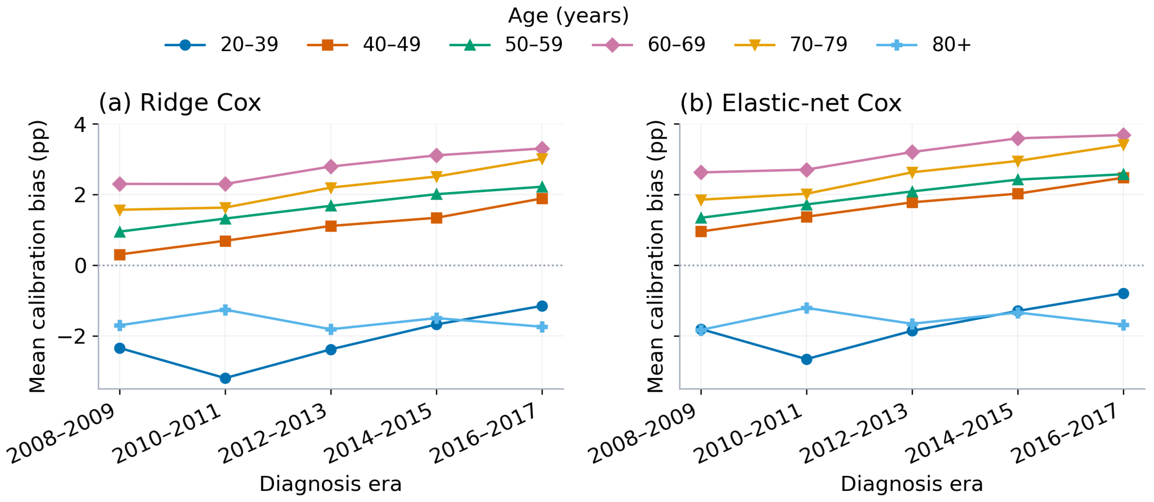
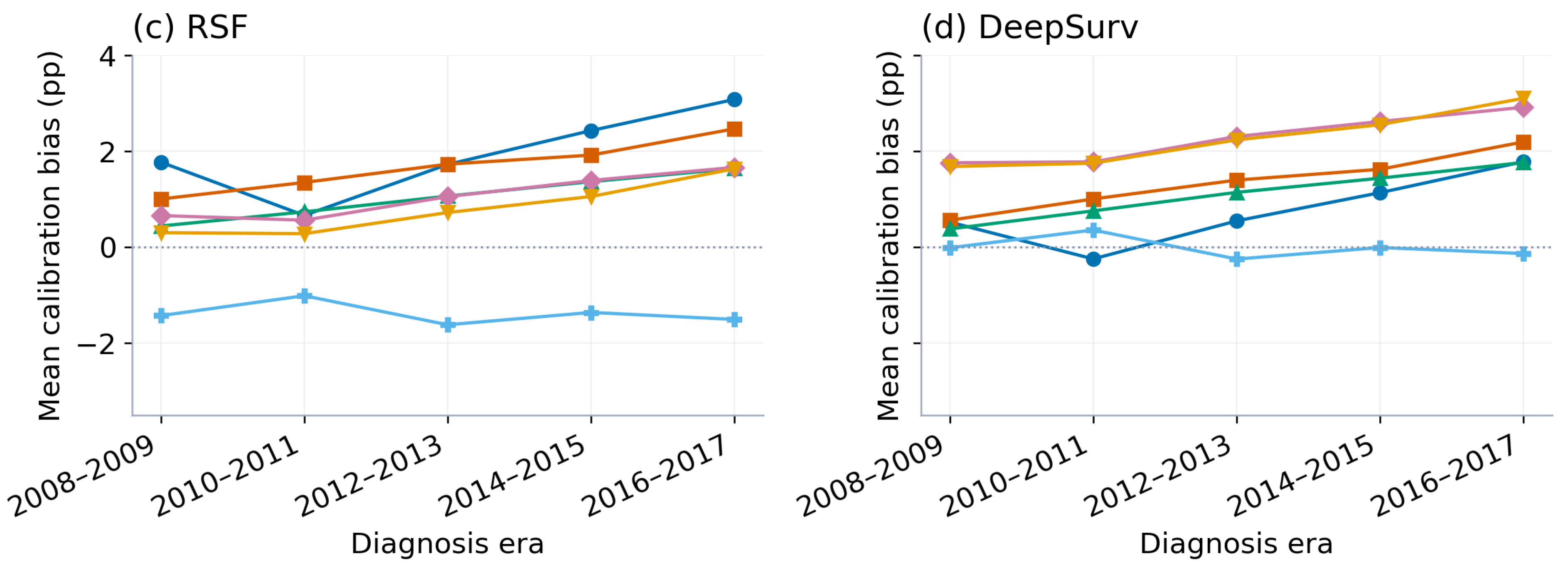
Figure A3.
Mean calibration bias by predicted-risk decile in the first and latest evaluation eras: (a) ridge Cox, (b) elastic-net Cox, (c) RSF, and (d) DeepSurv. Positive values indicate overprediction and negative values indicate underprediction. The two eras contain distinct patients; deciles are defined within each family and era. Values are supplied in Supplementary Table S8.
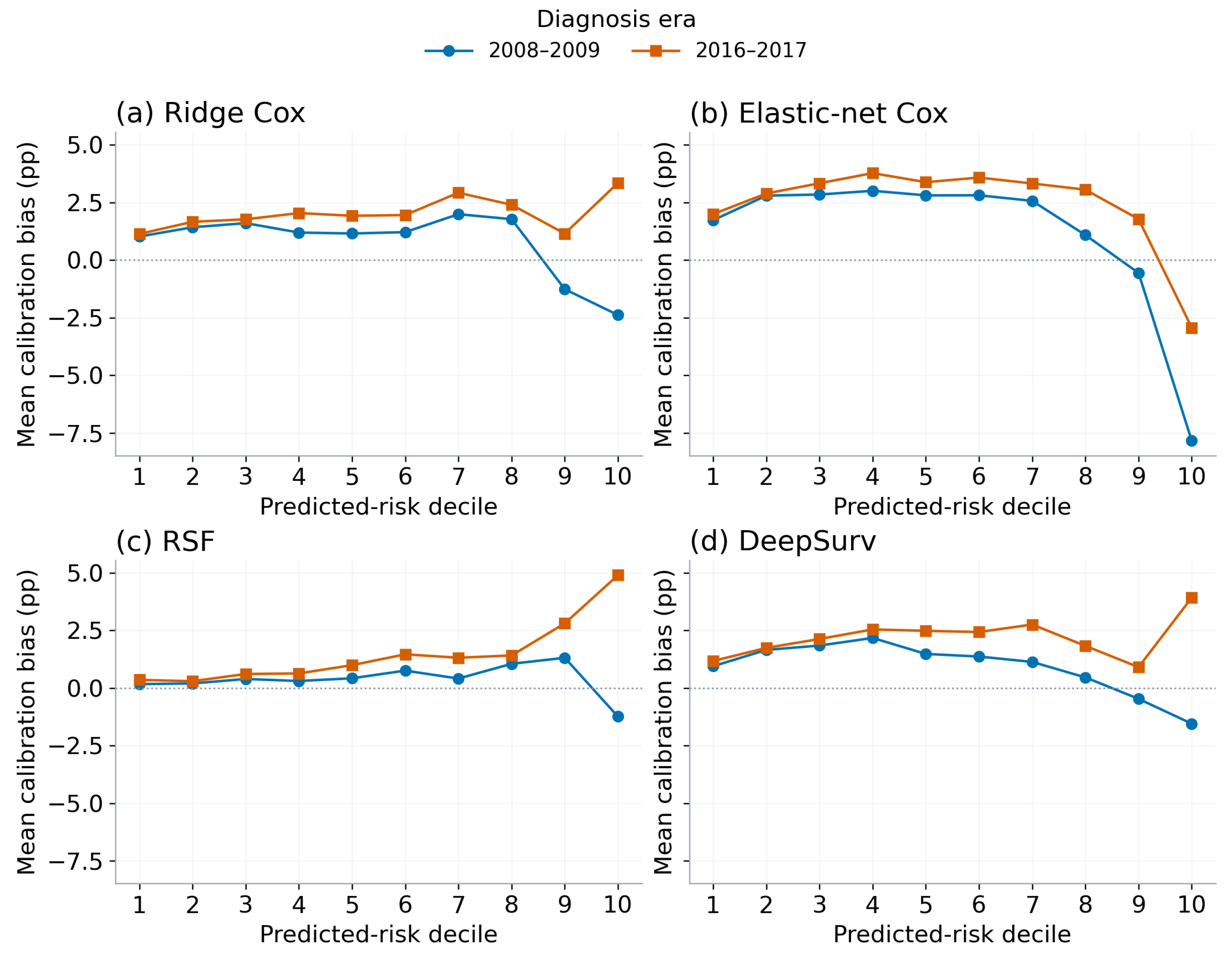
Figure A4.
Decision curves across BCSM risk thresholds from 2.5% to 30%: (a) ridge Cox, (b) elastic-net Cox, (c) RSF, and (d) DeepSurv. Curves compare fixed prediction in the first era with fixed and recalibrated prediction in the latest era, using distinct diagnosis cohorts. Net benefit refers to a hypothetical action with unspecified intervention benefit.
References
- Wishart, G.C.; Azzato, E.M.; Greenberg, D.C.; Rashbass, J.; Kearins, O.; Lawrence, G.; Caldas, C.; Pharoah, P.D.P. PREDICT: A new UK prognostic model that predicts survival following surgery for invasive breast cancer. Breast Cancer Res. 2010, 12, R1. [Google Scholar] [CrossRef] [Scilit] [PubMed]
- Collins, G.S.; Dhiman, P.; Ma, J.; Schlussel, M.M.; Archer, L.; Van Calster, B.; Harrell, F.E.; Martin, G.P.; Moons, K.G.M.; van Smeden, M.; et al. Evaluation of clinical prediction models (part 1): From development to external validation. BMJ 2024, 384, e074819. [Google Scholar] [CrossRef] [Scilit] [PubMed]
- van Houwelingen, H.C. Validation, calibration, revision and combination of prognostic survival models. Stat. Med. 2000, 19, 3401–3415. [Google Scholar] [CrossRef] [Scilit] [PubMed]
- Van Calster, B.; Nieboer, D.; Vergouwe, Y.; De Cock, B.; Pencina, M.J.; Steyerberg, E.W. A calibration hierarchy for risk models was defined: From utopia to empirical data. J. Clin. Epidemiol. 2016, 74, 167–176. [Google Scholar] [CrossRef] [Scilit] [PubMed]
- Davis, S.E.; Lasko, T.A.; Chen, G.; Matheny, M.E. Calibration Drift Among Regression and Machine Learning Models for Hospital Mortality. AMIA Annu. Symp. Proc. 2017, 2017, 625–634. [Google Scholar] [PubMed]
- Davis, S.E.; Greevy, R.A.; Lasko, T.A.; Walsh, C.G.; Matheny, M.E. Detection of calibration drift in clinical prediction models to inform model updating. J. Biomed. Inform. 2020, 112, 103611. [Google Scholar] [CrossRef] [Scilit] [PubMed]
- Cabanillas Silva, P.; Sun, H.; Rezk, M.; Roccaro-Waldmeyer, D.M.; Fliegenschmidt, J.; Hulde, N.; von Dossow, V.; Meesseman, L.; Depraetere, K.; Stieg, J.; et al. Longitudinal Model Shifts of Machine Learning–Based Clinical Risk Prediction Models: Evaluation Study of Multiple Use Cases Across Different Hospitals. J. Med. Internet Res. 2024, 26, e51409. [Google Scholar] [CrossRef] [Scilit] [PubMed]
- Ishwaran, H.; Kogalur, U.B.; Blackstone, E.H.; Lauer, M.S. Random survival forests. Ann. Appl. Stat. 2008, 2, 841–860. [Google Scholar] [CrossRef] [Scilit]
- Katzman, J.L.; Shaham, U.; Cloninger, A.; Bates, J.; Jiang, T.; Kluger, Y. DeepSurv: Personalized treatment recommender system using a Cox proportional hazards deep neural network. BMC Med. Res. Methodol. 2018, 18, 24. [Google Scholar] [CrossRef] [Scilit] [PubMed]
- Pölsterl, S. scikit-survival: A Library for Time-to-Event Analysis Built on Top of scikit-learn. J. Mach. Learn. Res. 2020, 21, 1–6. [Google Scholar]
- Abdikenov, B.; Zhaksylyk, T.; Imasheva, A.; Rakishev, D. From Mammogram Analysis to Clinical Integration with Deep Learning in Breast Cancer Diagnosis. Informatics 2025, 12, 106. [Google Scholar] [CrossRef] [Scilit]
- van Geloven, N.; Giardiello, D.; Bonneville, E.F.; Teece, L.; Ramspek, C.L.; van Smeden, M.; Snell, K.I.E.; Van Calster, B.; Pohar Perme, M.; Riley, R.D.; et al. Validation of prediction models in the presence of competing risks: A guide through modern methods. BMJ 2022, 377, e069249. [Google Scholar] [CrossRef] [Scilit] [PubMed]
- Van Calster, B.; Steyerberg, E.W.; Wynants, L.; van Smeden, M. There is no such thing as a validated prediction model. BMC Med. 2023, 21, 70. [Google Scholar] [CrossRef] [Scilit] [PubMed]
- Booth, S.; Riley, R.D.; Ensor, J.; Lambert, P.C.; Rutherford, M.J. Temporal recalibration for improving prognostic model development and risk predictions in settings where survival is improving over time. Int. J. Epidemiol. 2020, 49, 1316–1325. [Google Scholar] [CrossRef] [Scilit] [PubMed]
- Booth, S.; Mozumder, S.I.; Archer, L.; Ensor, J.; Riley, R.D.; Lambert, P.C.; Rutherford, M.J. Using temporal recalibration to improve the calibration of risk prediction models in competing risk settings when there are trends in survival over time. Stat. Med. 2023, 42, 5007–5024. [Google Scholar] [CrossRef] [Scilit] [PubMed]
- Tanner, K.T.; Diaz-Ordaz, K.; Keogh, R.H. Implementation of a dynamic model updating pipeline provides a systematic process for maintaining performance of prediction models. J. Clin. Epidemiol. 2024, 175, 111531. [Google Scholar] [CrossRef] [Scilit] [PubMed]
- Clift, A.K.; Dodwell, D.; Lord, S.; Petrou, S.; Brady, M.; Collins, G.S.; Hippisley-Cox, J. Development and internal-external validation of statistical and machine learning models for breast cancer prognostication: Cohort study. BMJ 2023, 381, e073800. [Google Scholar] [CrossRef] [Scilit] [PubMed]
- Janssen, K.J.M.; Moons, K.G.M.; Kalkman, C.J.; Grobbee, D.E.; Vergouwe, Y. Updating methods improved the performance of a clinical prediction model in new patients. J. Clin. Epidemiol. 2008, 61, 76–86. [Google Scholar] [CrossRef] [Scilit] [PubMed]
- Hsiao, Y.W.; Wishart, G.C.; Pharoah, P.D.P.; Peng, P.C. Assessing the Performance of the PREDICT Breast Version 3.0 Prognostic Tool in Patients With Breast Cancer in the United States. J. Natl. Compr. Cancer Netw. 2025, 23, 227–233. [Google Scholar] [CrossRef] [Scilit] [PubMed]
- Verheul, E.M.; Doornkamp, F.; Petrov, I.; Siesling, S.; Lingsma, H.F.; Koppert, L.B.; Vreven, L.W.A.; Voogd, A.C.; Karsten, M.M.; Doppelbauer, L.; et al. External validation of PREDICT Breast v3.1 for overall survival in international cohorts, including young and invasive lobular subgroups. Breast Cancer Res. Treat. 2026, 217, 14. [Google Scholar] [CrossRef] [Scilit] [PubMed]
- Tanner, K.T.; Keogh, R.H.; Coupland, C.A.C.; Hippisley-Cox, J.; Diaz-Ordaz, K. Dynamic updating of clinical survival prediction models in a changing environment. Diagn. Progn. Res. 2023, 7, 24. [Google Scholar] [CrossRef] [Scilit] [PubMed]
- Feng, J.; Gossmann, A.; Sahiner, B.; Pirracchio, R. Bayesian logistic regression for online recalibration and revision of risk prediction models with performance guarantees. J. Am. Med. Inform. Assoc. 2022, 29, 841–852. [Google Scholar] [CrossRef] [Scilit] [PubMed]
- National Cancer Institute. Surveillance, Epidemiology, and End Results (SEER) Program: SEER Research Data, 17 Registries, November 2025 Submission (2000–2023) [Dataset]. Released April 2026; Data Description Updated April 2026; Administrative Follow-Up Cut-Off: 31 December 2023. Available online: https://seer.cancer.gov/data-software/documentation/seerstat/nov2025/ (accessed on 6 October 2026).
- Vickers, A.J.; Elkin, E.B. Decision curve analysis: A novel method for evaluating prediction models. Med. Decis. Mak. 2006, 26, 565–574. [Google Scholar] [CrossRef] [Scilit] [PubMed]
- Sadatsafavi, M.; Adibi, A.; Puhan, M.; Gershon, A.; Aaron, S.D.; Sin, D.D. Moving beyond AUC: Decision curve analysis for quantifying net benefit of risk prediction models. Eur. Respir. J. 2021, 58, 2101186. [Google Scholar] [CrossRef] [Scilit] [PubMed]
- Austin, P.C.; Harrell, F.E.; van Klaveren, D. Graphical calibration curves and the integrated calibration index (ICI) for survival models. Stat. Med. 2020, 39, 2714–2742. [Google Scholar] [CrossRef] [Scilit] [PubMed]
- Austin, P.C.; Putter, H.; Giardiello, D.; van Klaveren, D. Graphical calibration curves and the integrated calibration index (ICI) for competing risk models. Diagn. Progn. Res. 2022, 6, 2. [Google Scholar] [CrossRef] [Scilit] [PubMed]
- Wolbers, M.; Koller, M.T.; Witteman, J.C.M.; Steyerberg, E.W. Prognostic Models with Competing Risks: Methods and Application to Coronary Risk Prediction. Epidemiology 2009, 20, 555–561. [Google Scholar] [CrossRef] [Scilit] [PubMed]
- Wolbers, M.; Blanche, P.; Koller, M.T.; Witteman, J.C.M.; Gerds, T.A. Concordance for prognostic models with competing risks. Biostatistics 2014, 15, 526–539. [Google Scholar] [CrossRef] [Scilit] [PubMed]
- Gerds, T.A.; Andersen, P.K.; Kattan, M.W. Calibration plots for risk prediction models in the presence of competing risks. Stat. Med. 2014, 33, 3191–3203. [Google Scholar] [CrossRef] [Scilit] [PubMed]
- Wishart, G.C.; Bajdik, C.D.; Dicks, E.; Provenzano, E.; Schmidt, M.K.; Sherman, M.; Greenberg, D.C.; Green, A.R.; Gelmon, K.A.; Kosma, V.M.; et al. PREDICT Plus: Development and validation of a prognostic model for early breast cancer that includes HER2. Br. J. Cancer 2012, 107, 800–807. [Google Scholar] [CrossRef] [Scilit] [PubMed]
- Candido dos Reis, F.J.; Wishart, G.C.; Dicks, E.M.; Greenberg, D.; Rashbass, J.; Schmidt, M.K.; van den Broek, A.J.; Ellis, I.O.; Green, A.; Rakha, E.; et al. An updated PREDICT breast cancer prognostication and treatment benefit prediction model with independent validation. Breast Cancer Res. 2017, 19, 58. [Google Scholar] [CrossRef] [Scilit] [PubMed]
- Gray, E.; Marti, J.; Brewster, D.H.; Wyatt, J.C.; Hall, P.S. Independent validation of the PREDICT breast cancer prognosis prediction tool in 45,789 patients using Scottish Cancer Registry data. Br. J. Cancer 2018, 119, 808–814. [Google Scholar] [CrossRef] [Scilit] [PubMed]
- Stabellini, N.; Cao, L.; Towe, C.W.; Miller, M.E.; Sousa-Santos, A.H.; Amin, A.B.; Montero, A.J. Validation of the PREDICT Prognostication Tool in US Patients With Breast Cancer. J. Natl. Compr. Cancer Netw. 2023, 21, 1011–1019.e6. [Google Scholar] [CrossRef] [Scilit] [PubMed]
- Wang, Y.; Broeks, A.; Giardiello, D.; Hauptmann, M.; Jóźwiak, K.; Koop, E.A.; Opdam, M.; Siesling, S.; Sonke, G.S.; Stathonikos, N.; et al. External validation and clinical utility assessment of PREDICT breast cancer prognostic model in young, systemic treatment-naïve women with node-negative breast cancer. Eur. J. Cancer 2023, 195, 113401. [Google Scholar] [CrossRef] [Scilit] [PubMed]
- Grootes, I.; Wishart, G.C.; Pharoah, P.D.P. An updated PREDICT breast cancer prognostic model including the benefits and harms of radiotherapy. npj Breast Cancer 2024, 10, 6. [Google Scholar] [CrossRef] [Scilit] [PubMed]
- Vreven, L.W.A.; Verheul, E.M.; van Maaren, M.C.; Doornkamp, F.; Schipper, R.J.; Siesling, S.; Pharoah, P.D.P.; Tjan-Heijnen, V.C.G.; Voogd, A.C. Comparative validation of PREDICT versions 3.1 and 2.2 for overall survival in the Dutch breast cancer population. Breast 2026, 85, 104681. [Google Scholar] [CrossRef] [Scilit] [PubMed]
- Pharoah, P.D.P.; Hsiao, Y.W.; Wishart, G.C.; Peng, P.C. PREDICT breast v4.0: An update to the PREDICT breast prognostic model. BMC Res. Notes 2025, 18, 482. [Google Scholar] [CrossRef] [Scilit] [PubMed]
- Chen, E.; Chen, C.; Chen, Y.; You, J.; Jin, C.; Huang, Z.; Zhang, J.; Wang, Q.; Cai, Y.; Hu, X.; et al. Insights into the performance of PREDICT tool in a large Mainland Chinese breast cancer cohort: A comparative analysis of versions 3.0 and 2.2. Oncologist 2024, 29, e976–e983. [Google Scholar] [CrossRef] [Scilit] [PubMed]
- Collins, G.S.; Moons, K.G.M.; Dhiman, P.; Riley, R.D.; Beam, A.L.; Van Calster, B.; Ghassemi, M.; Liu, X.; Reitsma, J.B.; van Smeden, M.; et al. TRIPOD+AI statement: Updated guidance for reporting clinical prediction models that use regression or machine learning methods. BMJ 2024, 385, e078378. [Google Scholar] [CrossRef] [Scilit] [PubMed]

Disclaimer/Publisher’s Note: The statements, opinions and data contained in all publications are solely those of the individual author(s) and contributor(s) and not of MDPI and/or the editor(s). MDPI and/or the editor(s) disclaim responsibility for any injury to people or property resulting from any ideas, methods, instructions or products referred to in the content. |
© 2026 by the authors. Licensee MDPI, Basel, Switzerland. This article is an open access article distributed under the terms and conditions of the Creative Commons Attribution (CC BY) license.